Theory and implementation of Complex-Valued Neural Networks

Abstract

This work explains in detail the theory behind Complex-Valued Neural Network (CVNN), including Wirtinger calculus, complex backpropagation and basic modules such as complex layers, complex activation functions or complex weight initialization. We also show the impact of not adapting the weight initialization correctly to the complex domain. This work presents a strong focus on the implementation of such modules on Python using cvnn toolbox. We also perform simulations on real-valued data, casting to the complex domain by means of the Hilbert Transform and verify the potential interest of CVNN even for non-complex data.

Keywords CVNN  $\cdot$ Deep Learning  $\cdot$ Complex values  $\cdot$ Machine Learning

1 Introduction

Although CVNN has been investigated for particular structures of complex-valued data [1, 2, 3, 4], the difficulties in implementing CVNN models in practice have slowed down the field from growing further [5]. Indeed, the two most popular Python libraries for developing deep neural networks, which are Pytorch, from Meta (formerly named Facebook) and Tensorflow from Google do not fully support the creation of complex-valued models.

Even though Tensorflow does not fully support the implementation of a CVNN, it has one significant benefit: It enables the use of complex-valued data types for the automatic differentiation (autodiff)algorithm [6] to calculate the complex gradients as defined in Appendix C. Since July 2020, PyTorch also added this functionality as BETA with the version 1.6 release. later on, on June 2022, after the release of version 1.12, PyTorch extended its complex functionality by adding complex convolutions (also as BETA). Although this indicates a clear intention to develop towards CVNN support, there is still a lot of development to be done.

Libraries to develop CVNN s do exist, the most important one of them being probably the code published in [7]. However, we have decided not to use this library since the latter uses Theano as a back-end, which is no longer maintained. Another code was published on GitHub that uses Tensorflow and Keras to implement CVNN [8]. However, as Keras does not support complex-valued numbers, the published code simulates complex operations using real-valued datatypes. Therefore, the user has to transform its complex-valued data into a real-valued equivalent before using this library. The same happened with ComplexPyTorch [9] until it was updated in January 2021 to support complex tensors.

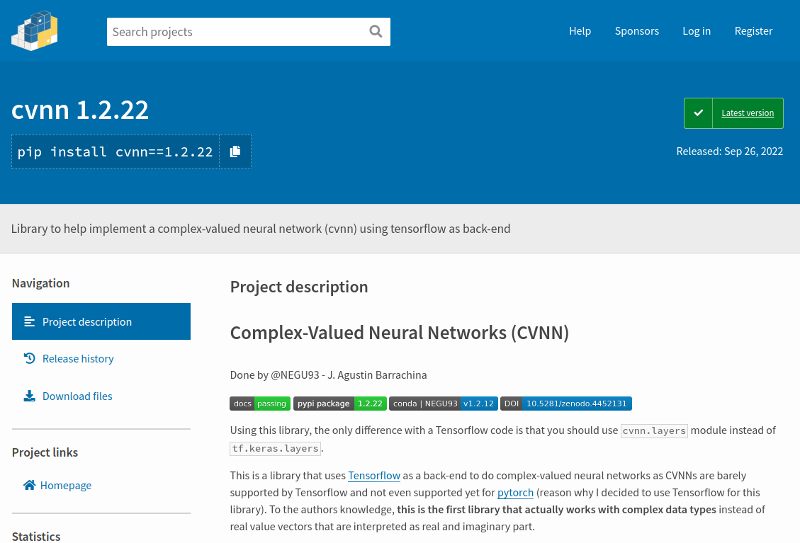
((a)) PIP cvnn presentation page.

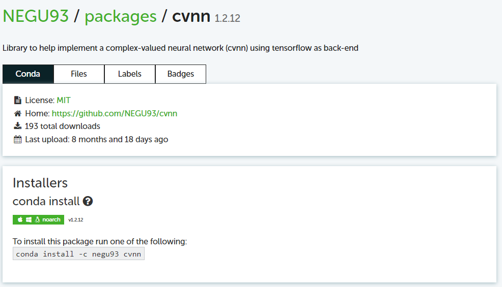
((b)) Anaconda cvnn presentation page.

During this thesis, we created a Python tool to deal with the implementation of CVNN models using Tensorflow as back-end. Note that the development of this library started in 2019, whereas PyTorch support for complex numbers started in mid-2020, which is the reason why the decision to use Tensorflow instead of Pytorch was made. To the author’s knowledge, this was the first library that natively supported complex-number data types. The library is called CVNN and was published [10] using CERN’s Zenodo platform which received already 18 downloads. It can be installed using both Python Index Package (PIP) (Figure 1(a)) and Anaconda. The latter already has 193 downloads as of the $8^{\text{th}}$ October 2022, as shown in Figure 1(b), from which none of those downloads were ourselves.

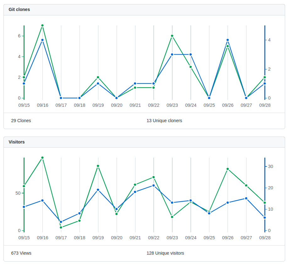
Figure 2: GitHub cvnn toolbox traffic.

The library was open-sourced for the community on GitHub [11] and has received a very positive reception from the community. As can be seen from Figure 2, the GitHub repository received an average of 2 clones and almost 50 visits per day in the last two weeks. With 62 stars at the beginning of October 2022. It also has a total of 16 forks and one pull request for a new feature that has already been reviewed and accepted. Six users are actively watching every update on the code as they have activated the notifications. Finally, two users have codes in GitHub importing the library. Thirty issues have been reported, and it was also subject to 31 private emails. All these metrics are evidence of the impact and interest of the community in the published code.

The library was documented using reStructuredText and uploaded for worldwide availability. The link for the full documentation (displayed in Figure 3(a)) can be found in the following link: complex-valued-neural-networks.rtfd.io. The documentation received a daily view which varied from a minimum of 18 views on one day to a maximum of 173 views as shown in Figure 3(b)

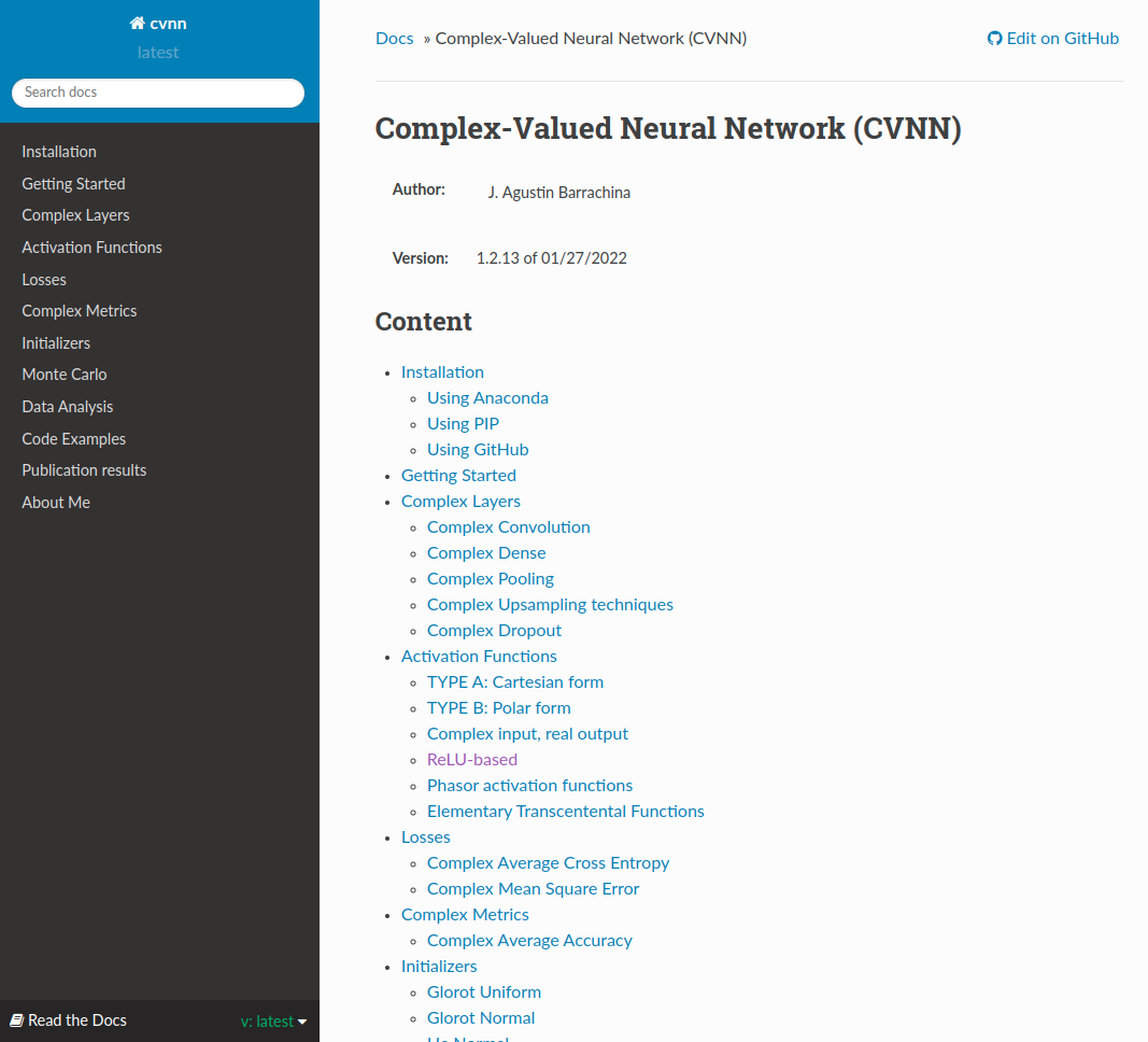
((a)) Read the Docs documentation presentation page.

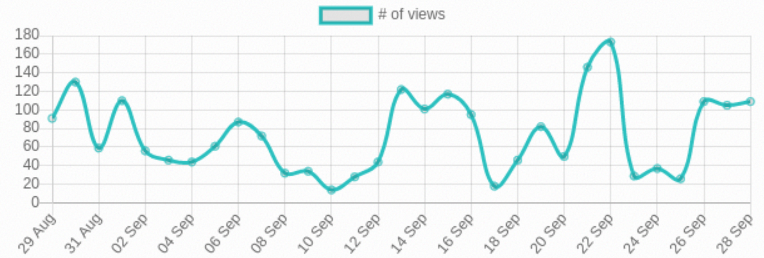
((b)) cvnn documentation daily total views in Read The Docs.

Figure 3: Documentation hosted by Read the Docs.

The Python testing framework Pytest was used to maintain a maximum degree of quality and keep it as bug-free as possible. Before each new feature implementation, a test module was created to assert the expected behavior of the feature and reduce bugs to a minimum. This methodology also guaranteed feature compatibility as all designed test modules must pass in order to deploy the code. The library allows the implementation of a Real-Valued Neural Network (RVNN)as well with the intention of changing as little as possible the code when using complex data types. This made it possible to perform a straight comparison against Tensorflow’s models, which helped in the debugging. Indeed, some Pytest modules achieved the same result that Tensorflow when initializing the models with the same seed.

Special effort was made on the User eXperience (UX)by keeping the Application Programming Interface (API)as similar as possible to that of Tensorflow. The following code extract would work both for a Tensorflow or cvnn application code:

⬇

1import numpy as np

2import tensorflow as tf

3

4# Gets the dataset, when using cvnn you normally want this to be complex

5# for example numpy arrays of dtype np.complex64

6# to be done by each user

7(train_images, train_labels), (test_images, test_labels) = get_dataset()

8

9# This function returns a tf.Model object

10model = get_model()

11

12# Compile as any TensorFlow model

13model.compile(optimizer=’adam’, metrics=[’accuracy’], loss=tf.keras.losses.SparseCategoricalCrossentropy(from_logits=True))

14model.summary()

15

16# Train and evaluate

17history = model.fit(train_images, train_labels, epochs=epochs, validation_data=(test_images, test_labels))

18test_loss, test_acc = model.evaluate(test_images, test_labels, verbose=2)

For creating the model, two API s are available, the first one known as the sequential API whose usage is something like the following code extract:

⬇

1import cvnn.layers as layers

2

3def get_model():

4 model = tf.keras.models.Sequential()

5 model.add(layers.ComplexInput(input_shape=(32, 32, 3)))

6 model.add(layers.ComplexConv2D(32, (3, 3), activation=’cart_relu’))

7 model.add(layers.ComplexAvgPooling2D((2, 2)))

8 model.add(layers.ComplexConv2D(64, (3, 3), activation=’cart_relu’))

9 model.add(layers.ComplexMaxPooling2D((2, 2)))

10 model.add(layers.ComplexConv2D(64, (3, 3), activation=’cart_relu’))

11 model.add(layers.ComplexFlatten())

12 model.add(layers.ComplexDense(64, activation=’cart_relu’))

13 model.add(layers.ComplexDense(10, activation=’convert_to_real_with_abs’))

14 # An activation that casts to real must be used at the last layer.

15 # The loss function cannot minimize a complex number

16 return model

However, some models are simply impossible to create with the sequential API like a U-NET architecture. For that, the functional API must be used like this:

⬇

1import cvnn.layers as layers

2

3def get_model():

4 inputs = layers.complex_input(shape=(128, 128, 3))

5 c0 = layers.ComplexConv2D(32, activation=’cart_relu’, kernel_size=3)(inputs)

6 c1 = layers.ComplexConv2D(32, activation=’cart_relu’, kernel_size=3)(c0)

7 c2 = layers.ComplexMaxPooling2D(pool_size=(2, 2), strides=(2, 2), padding=’valid’)(c1)

8 t01 = layers.ComplexConv2DTranspose(5, kernel_size=2, strides=(2, 2), activation=’cart_relu’)(c2)

9 concat01 = tf.keras.layers.concatenate([t01, c1], axis=-1)

10

11 c3 = layers.ComplexConv2D(4, activation=’cart_relu’, kernel_size=3)(concat01)

12 out = layers.ComplexConv2D(4, activation=’cart_relu’, kernel_size=3)(c3)

13 return tf.keras.Model(inputs, out)

When using Keras loss functions, the output of the model must be real-valued as Tensorflow will not work with complex values. There are activation functions defined that receive complex values as input but output real value results to deal with this problem. Another solution is to use the cvnn library-defined loss functions instead.

Tensorflow blocks the use of a complex-valued loss as the optimizer input but allows the update over complex-valued trainable parameters by means of the Wirtinger calculus (Appendix 2.2). As the loss is real-valued, the optimizer can be the same as the one used for real-valued networks, so no implementation was needed in this regard. However, the other modules must be implemented. Their detail will be described in the following Sections.

2 Mathematical Background

The beginning of CVNN was deferred mainly because of Liouville’s theorem, which stated that a bounded and differentiable throughout all the complex domain is then a constant function, forcing the loss function to be non-holomorphic. Liouville’s theorem implications were considered to be a big problem around 1990 as some researchers believed indifferentiability should lead to the impossibility to obtain and/or analyze the dynamics of the CVNN s [12]. Later Wirtinger calculus proposed a gradient definition for non-holomorphic functions and is now widely used for optimizing and training complex models.

2.1 Liouville Theorem

Liouville graduated from the École Polytechnique in 1827. After some years as an assistant at various institutions including the École Centrale Paris, he was appointed as a professor at the École Polytechnique in 1838.

Definition 2.1.

In complex analysis, an entire function, also called an integral function, is a complex-valued function that is holomorphic at all finite points over the whole complex plane.

Definition 2.2.

Given a function $f$, the function is bounded if $\exists M\in\mathbb{R^{+}}:|f(z)|<M$.

Theorem 2.1 (Cauchy integral theorem).

Given $f$ analytic through region D, then the contour integral of $f(z)$ along any close path $C$ inside region D is zero:

$$\oint_{C}f(z)dz=0\,.$$ (1)

Theorem 2.2 (Cauchy integral formula).

Given $f$ analytic on the boundary $C$ with $z_{0}$ any point inside $C$, then:

$$f(z_{0})=\frac{1}{2\pi i}\oint_{C}\frac{f(z)}{z-z_{0}}\,dz\,,$$ (2)

where the contour integration is taken in the counterclockwise direction.

Corollary 2.2.1.

$$f^{(n)}(z_{0})=\frac{n!}{2\pi i}\oint_{C}\frac{f(z)}{(z-z_{0})^{n+1}}\,dz\,.$$ (3)

In complex analysis, Liouville’s theorem states that every bounded entire function must be constant. That is:

Theorem 2.3 (Liouville’s Theorem).

$$f:\mathbb{C}\longrightarrow\mathbb{C}\text{ holomorphic }/\exists M\in\mathbb{R^{+}}:\left|f(z)\right|<M,\forall z\in\mathbb{C}\Rightarrow f=c,c\in\mathbb{C}\,.$$ (4)

Equivalently, non-constant holomorphic functions on $\mathbb{C}$ have unbounded images.

Proof.

Because every holomorphic function is analytic (Class $C^{\infty}$), that is, it can be represented as a Taylor series, we can therefore write it as:

$$f(z)=\sum_{k=0}^{\infty}a_{k}\,z^{k}\,.$$ (5)

As $f$ is holomorphic in the open region enclosed by the path and continuous on its closure. Because of 3 we have:

$$a_{k}=\frac{f^{(k)}(0)}{k!}=\frac{1}{2\pi i}\oint_{C_{r}}\frac{f(z)}{z^{k+1}dz}\,,$$ (6)

where $C_{r}$ is a circle of radius $r>0$. Because $f$ is bounded:

$$\left|a_{k}\right|\leqslant\frac{1}{2\pi}\oint_{C_{r}}\frac{\left|f(z)\right|}{\left|z\right|^{k+1}}\left|dz\right|\leqslant\frac{1}{2\pi}\oint_{C_{r}}\frac{M}{r^{k+1}}\left|dz\right| =\frac{M}{2\pi r^{k+1}}\oint_{C_{r}}\left|dz\right|\,,$$ (7)

$$=\frac{M}{2\pi r^{k+1}}2\pi\,,$$ (8)

$$=\frac{M}{r^{k}}\,.$$ (9)

The latest derivation is also known as Cauchy’s inequality.

As $r$ is any positive real number, by taking the $r\to\infty$ then $a_{k}\to 0$ for all $k\neq 0$. Therefore from Equation 5 we have that $f(z)=a_{0}$. ∎

2.2 Wirtinger Calculus

Wirtinger calculus, named after Wilhelm Wirtinger (1927) [13], generalizes the notion of complex derivative, and the holomorphic functions become a special case only. Further reading on Wirtinger calculus can be found in [14, 15].

Theorem 2.4 (Wirtinger Calculus).

Given a complex function $f(z)$ of a complex variable $z=x+i\,y\in\mathbb{C},x,y\in\mathbb{R}$.

The partial derivatives with respect to $z$ and $\overline{z}$ respectively are defined as:

$$\frac{\partial f}{\partial z}\triangleq\frac{1}{2}\left(\frac{\partial f}{\partial x}-i\,\frac{\partial f}{\partial y}\right)\,,$$ (10)

$$\frac{\partial f}{\partial\overline{z}}\triangleq\frac{1}{2}\left(\frac{\partial f}{\partial x}+i\,\frac{\partial f}{\partial y}\right)\,.$$

These derivatives are called $\mathbb{R}$-derivative and conjugate $\mathbb{R}$-derivative, respectively. As said before, the holomorphic case is only a special case where the function can be considered as $f(z,\overline{z}),\overline{z}=0$. Wirtinger calculus enables to work with non-holomorphic functions, providing an alternative method for computing the gradient that also improves the stability of the training process.

Proof.

Defining $z=x+i\,y$ one can also define $x(z,\overline{z}),y(z,\overline{z}):\mathbb{C}\longrightarrow\mathbb{R}$ as follows:

$$x =\frac{1}{2}\left(z+\overline{z}\right)\,,$$ (11)

$$y =\frac{1}{2\,i}\left(z-\overline{z}\right)\,.$$

Using (A.4):

$$\frac{\partial f}{\partial z} =\frac{\partial f}{\partial x}\frac{\partial x}{\partial z}+\frac{\partial f}{\partial y}\frac{\partial y}{\partial z}\,,$$ (12)

$$=\frac{\partial f}{\partial x}\frac{1}{2}+\frac{\partial f}{\partial y}\left(\frac{-i}{2}\right)\,,$$

$$=\frac{1}{2}\left(\frac{\partial f}{\partial x}-i\,\frac{\partial f}{\partial y}\right)\,.$$

∎

Corollary 2.4.1.

$$\frac{\partial f}{\partial g}+\frac{\partial f}{\partial\overline{g}} =\frac{1}{2}\left(\frac{\partial f}{\partial g_{\mathrm{Re}{}}}-i\,\frac{\partial f}{\partial g_{\mathrm{Im}{}}}\right)+\frac{1}{2}\left(\frac{\partial f}{\partial g_{\mathrm{Re}{}}}+i\,\frac{\partial f}{\partial g_{\mathrm{Im}{}}}\right)\,,$$ (13)

$$=\frac{\partial f}{\partial g_{\mathrm{Re}{}}}$$

$$i\left(\frac{\partial f}{\partial g}-\frac{\partial f}{\partial\overline{g}}\right) =\frac{i}{2}\left(\frac{\partial f}{\partial g_{\mathrm{Re}{}}}-i\,\frac{\partial f}{\partial g_{\mathrm{Im}{}}}\right)-\frac{i}{2}\left(\frac{\partial f}{\partial g_{\mathrm{Re}{}}}+i\,\frac{\partial f}{\partial g_{\mathrm{Im}{}}}\right)\,,$$

$$=\frac{i}{2}\left(-2i\,\frac{\partial f}{\partial g_{\mathrm{Im}{}}}\right)\,,$$

$$=\frac{\partial f}{\partial g_{\mathrm{Im}{}}}\,,$$

where $g_{\mathrm{Re}}{}$ and $g_{\mathrm{Im}}{}$ are the real and imaginary part of $g$ respectively.

Theorem 2.5.

Given $f:\mathbb{C}\longrightarrow\mathbb{C}$ holomorphic with $f(x+iy)=u(x,y)+iv(x,y)$ where $u,v:\mathbb{R}\longrightarrow\mathbb{R}$ real-differentiable functions. Then

$$\frac{\partial f}{\partial\overline{z}}=0\,.$$

Proof.

Using Wirtinger calculus (Section 2.2).

$$\frac{\partial f}{\partial\overline{z}}=\frac{1}{2}\left(\frac{\partial f}{\partial x}+i\,\frac{\partial f}{\partial y}\right)\,.$$ (14)

By definition, then:

$$\frac{\partial f}{\partial\overline{.}} =\frac{1}{2}\left(\frac{\partial f}{\partial x}+i\,\frac{\partial f}{\partial y}\right)\,,$$ (15)

$$=\frac{1}{2}\left(\left(\frac{\partial u}{\partial x}+i\,\frac{\partial v}{\partial x}\right)+i\,\left(\frac{\partial u}{\partial y}+i\,\frac{\partial v}{\partial y}\right)\right)\,,$$

$$=\frac{1}{2}\left(\left(\frac{\partial u}{\partial x}-\frac{\partial v}{\partial y}\right)+i\,\left(\frac{\partial v}{\partial x}+\frac{\partial u}{\partial y}\right)\right)\,.$$

Because $f$ is holomorphic then the Cauchy-Riemann equations (Theorem 78) applies making Equation 15 equal to zero. ∎

Even though so far we have always talked about general chain rule definitions. Here we will demonstrate a particularly interesting chain rule used when working with neural networks. For this optimization technique, the cost function to optimize is always real, even if its variables are not. Therefore, the following chain rule will have an application interest.

Theorem 2.6 (complex chain rule with real output).

Given $f:\mathbb{C}\to\mathbb{R}$, $g:\mathbb{C}\to\mathbb{C}$ with $g(z)=r(z)+i\,s(z)$, $z=x+i\,y\in\mathbb{C}$:

$$\frac{\partial f}{\partial z}=\frac{\partial f}{\partial r}\frac{\partial r}{\partial z}+\frac{\partial f}{\partial s}\frac{\partial s}{\partial z}\,.$$ (16)

Proof.

For this proof, we will assume we are already working with Wirtinger Calculus for the partial derivative definition.

$$\frac{\partial f}{\partial z} =\frac{\partial f}{\partial g}\frac{\partial g}{\partial z}+\frac{\partial f}{\partial\overline{g}}\frac{\partial\overline{g}}{\partial z}\,,$$ (17)

$$=\frac{1}{4}\left(\frac{\partial f}{\partial r}-i\,\frac{\partial f}{\partial s}\right)\left(\frac{\partial g}{\partial x}-i\,\frac{\partial g}{\partial y}\right)+\frac{1}{4}\left(\frac{\partial f}{\partial r}+i\,\frac{\partial f}{\partial s}\right)\overline{\left(\frac{\partial g}{\partial x}+i\,\frac{\partial g}{\partial y}\right)}\,,$$

$$=\frac{1}{4}\left(\frac{\partial f}{\partial r}-i\,\frac{\partial f}{\partial s}\right)\left[\left(\frac{\partial r}{\partial x}+i\,\frac{\partial s}{\partial x}\right)-i\,\left(\frac{\partial r}{\partial y}+i\,\frac{\partial s}{\partial y}\right)\right]+\cdots$$

$$\cdots+\frac{1}{4}\left(\frac{\partial f}{\partial r}+i\,\frac{\partial f}{\partial s}\right)\overline{\left[\left(\frac{\partial r}{\partial x}+i\,\frac{\partial s}{\partial x}\right)+i\,\left(\frac{\partial r}{\partial y}+i\,\frac{\partial s}{\partial y}\right)\right]}\,.$$

∎

2.3 Notation

A MLP can be represented generically by Figure 4. For that given multi-layered neural network, we define the following variables, which will be used in the following subsections and throughout our work:

• $0\leq l\leq L$ corresponds to the layer index where $L$ is the output layer index and 0 is the input layer index.

• $1\leq n\leq N_{l}$ the neuron index, where $N_{l}$ denotes the number of neurons of layer $l$.

• $\omega^{(l)}_{nm}$ weight of the $n^{th}$ neuron of layer $l-1$ with the $m^{th}$ neuron of layer $l$.

• $\sigma$ activation function.

• $X_{n}^{(l)}=\sigma\left(V_{n}^{(l)}\right)$   considered the output of layer $l$ and input of layer $l+1$, in particular, $X_{n}^{(L)}=y_{n}$. With $V_{n}^{(l)}$ being

• $V_{n}^{(l)}=\displaystyle\sum_{m=1}^{N_{l-1}}\omega^{(l)}_{nm}X_{m}^{(l-1)}$

• $e_{n}(d_{n},y_{n})$ error function. $d_{n}$ is the desired output for neuron $n$ of the output layer.

• $\mathcal{L}=\displaystyle\sum_{n}^{N_{L}}e_{n}$ cost or loss function.

• $E=\displaystyle\frac{1}{P}\sum_{p}^{P}\mathcal{L}_{p}$   minimum error function, with $P$ the total number of training cases or the size of the desired batch size.

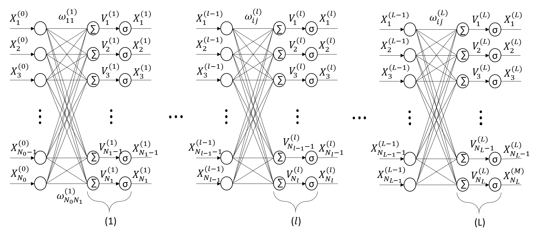
Figure 4: Feed-forward Neural Network Diagram.

2.4 Complex-Valued Backpropagation

The loss function remains real-valued to minimize an empirical risk during the learning process. Despite the architectural change for handling complex-valued inputs, the main challenge of CVNN is the way to train such neural networks.

A problem arises when implementing the learning algorithm (commonly known as backpropagation). The parameters of the network must be optimized using the gradient or any partial-derivative-based algorithm. However, standard complex derivatives only exist for the so-called holomorphic or analytic functions.

Because of Liouville’s theorem (discussed in Section 2.1), CVNN s are bound to use non-holomorphic functions and therefore can not be derived using standard complex derivative definition. CVNN s bring in non-holomorphic functions in at least two ways [16]:

• with the loss function being minimize over complex parameters

• with the non-holomorphic complex-valued activation functions

Liouville’s theorem implications were considered to be a big problem around 1990 as some researchers believed it led to the impossibility of obtaining and/or analyzing the dynamics of the CVNN s [12].

However, Wirtinger calculus (discussed in Section 2.2) generalizes the notion of complex derivative, making the holomorphic function a special case only, allowing researchers to successfully implement CVNN s. Under Wirtinger calculus, the gradient is defined as [17, 18]:

$$\nabla_{z}f=2\,\frac{\partial f}{\partial\overline{z}}\,.$$ (18)

When applying reverse-mode autodiff on the complex domain, some good technical reports can be found, such as [19] or [20]. However, it is left to be verified if Tensorflow correctly applies the equations mentioned in these reports. Indeed, no official documentation could be found that asserts the implementation of these equations and Wirtinger Calculus when using Tensorflow gradient on complex variables. This is not the case with PyTorch, where they explicitly say that Wirtinger calculus is used when computing the derivative in the following link: pytorch.org/docs/stable/notes/autograd.html. In said link, they indirectly say also that "This convention matches TensorFlow’s convention for complex differentiation […]" referencing the implementation of Equation 18.

However, we do know reverse-mode autodiff is the method used by Tensorflow [21]. When reverse engineering the gradient definition of Tensorflow, the conclusion discussed on the official Tensorflow’s GitHub repository issue report 3348 is that the gradient for $f:\mathbb{C}\to\mathbb{C}$ is computed as:

$$\nabla_{z}f=\overline{\left(\frac{\partial f}{\partial z}+\frac{\partial\overline{f}}{\partial z}\right)}=2\frac{\partial\mathrm{Re}(f)}{\partial\overline{z}}\,.$$ (19)

For application purposes, as the loss function is real-valued, we are only interested in cases where $f:\mathbb{C}^{n}\longrightarrow\mathbb{R}$ for what the above equation can be simplified as:

$$\nabla_{z}f=2\frac{\partial f}{\partial\overline{z}}=\left(\frac{\partial f}{\partial x}+i\frac{\partial f}{\partial y}\right)\,,$$ (20)

which indeed coincides with Wirtinger calculus definition. For this reason, it was not necessary to implement autodiff from scratch, and Tensorflow’s algorithm was used instead.

The mathematical equations on how to compute this figure are explained on Appendix B and it’s implementation for automatic calculation on a CPU or GPU is described in Appendix C.1 and C.2.

The analysis in the complex case is analogous to that made in the real-valued backpropagation on Appendix B. With the difference that now $\sigma:\mathbb{C}\longrightarrow\mathbb{C}$, $e_{n}:\mathbb{C}\longrightarrow\mathbb{R}$ and $\omega_{ij}^{(l)},X_{n}^{(l)},V_{n}^{(l)},e_{n}^{(l)}\in\mathbb{C}$.

Now, the chain rule is changed using (87) so Equation (94) changes to:

$$\frac{\partial e}{\partial\omega}=\frac{\partial e}{\partial X}\frac{\partial X}{\partial V}\frac{\partial V}{\partial\omega}+\frac{\partial e}{\partial X}\frac{\partial X}{\partial\overline{V}}\frac{\partial\overline{V}}{\partial\omega}+\frac{\partial e}{\partial\overline{X}}\frac{\partial\overline{X}}{\partial V}\frac{\partial V}{\partial\omega}+\frac{\partial e}{\partial\overline{X}}\frac{\overline{X}}{\partial\overline{V}}\frac{\partial\overline{V}}{\partial\omega}\,.$$ (21)

Note that we have used the upper line to denote the conjugate for clarity. All subindexes have been removed for clarity but they stand the same as in Equation 94.

As $e_{n}:\mathbb{C}\longrightarrow\mathbb{R}$ then using the conjugation rule (Definition A.3):

$$\frac{\partial e}{\partial\overline{X}} =\overline{\left(\frac{\partial e}{\partial X}\right)}\,,$$ (22)

$$\frac{\partial\overline{X}}{\partial\overline{V}} =\overline{\left(\frac{\partial X}{\partial V}\right)}\,,$$

$$\frac{\partial X}{\partial\overline{V}} =\overline{\left(\frac{\partial\overline{X}}{\partial V}\right)}\,,$$

so that not all the partial derivatives must be calculated.

Focusing our attention on the derivative $\partial V/\partial\omega$, a differentiation between layer difference of $V$ and $\omega$ will be made in this approach. The simplest is the one where the layer from $V_{n}^{(l)}$ is the same as the weight. Regardless of the complex domain, $V_{n}^{(l)}$ is still equal to $\displaystyle\sum_{i}^{N_{l-1}}\omega^{(l)}_{ni}X_{i}^{(l-1)}$ for what the value of the derivative remains unchanged. For the wights ($\omega$) of the previous layer, the derivative is as follows:

$$\frac{\partial V_{n}^{(l)}}{\partial\omega_{jk}^{(l-1)}} =\frac{\partial\left(\displaystyle\sum_{i}^{N_{l-1}}\omega^{(l)}_{n\mathrm{j}}X_{\mathrm{j}}^{(l-1)}\right)}{\partial\omega_{jk}^{(l-1)}}\,,$$ (23)

$$=\omega_{nj}^{(l)}\frac{\partial X_{j}^{(l-1)}}{\partial\omega_{jk}^{(l-1)}}\,,$$

$$=\omega_{nj}^{(l)}\left[\frac{\partial X_{j}^{(l-1)}}{\partial V_{j}^{(l-1)}}\frac{\partial V_{j}^{(l-1)}}{\partial\omega_{jk}^{(l-1)}}+\frac{\partial X_{j}^{(l-1)}}{\partial\overline{V}_{j}^{(l-1)}}\frac{\partial\overline{V}_{j}^{(l-1)}}{\partial\omega_{jk}^{(l-1)}}\right]\,.$$

Now by definition, $V_{n}^{(l)}$ is analytic because of being a polynomial series and therefore is holomorphic as well. Using Theorem 2.5, $\partial\overline{V}_{j}^{(l-1)}/\partial\omega_{jk}^{(l-1)}=0$. The second term could be removed. Therefore the equation is simplified to the following:

$$\frac{\partial V_{n}^{(l)}}{\partial\omega_{jk}^{(l-1)}}=\omega_{nj}^{(l)}\frac{\partial X_{j}^{(l-1)}}{\partial V_{j}^{(l-1)}}\frac{\partial V_{j}^{(l-1)}}{\partial\omega_{jk}^{(l-1)}}=\omega_{nj}^{(l)}\frac{\partial X_{j}^{(l-1)}}{\partial V_{j}^{(l-1)}}X_{k}^{(l-2)}\,.$$ (24)

For the rest of the cases where the layers are farther apart, the equation is as follows:

$$\frac{\partial V_{n}^{(l)}}{\partial\omega_{jk}^{(h)}} =\frac{\displaystyle\partial\left(\sum_{i}^{N_{l-1}}\omega^{(l)}_{ni}X_{i}^{(l-1)}\right)}{\partial\omega_{jk}^{(l-1)}}\,,$$ (25)

$$=\sum_{i}^{N_{l-1}}\omega_{nj}^{(l)}\left[\frac{\partial X_{i}^{(l-1)}}{\partial V_{i}^{(l-1)}}\frac{\partial V_{i}^{(l-1)}}{\partial\omega_{jk}^{(h)}}+\frac{\partial X_{i}^{(l-1)}}{\partial\overline{V}_{i}^{(l-1)}}\frac{\partial\overline{V}_{i}^{(l-1)}}{\partial\omega_{jk}^{(h)}}\right]\,,$$

where $h\leq l-2$. Therefore, based on Equations 25 and 24, the final equation remains as follows:

$$\frac{\partial V_{n}^{(l)}}{\partial\omega_{jk}^{(h)}}=\begin{cases}X_{j}^{(l-1)}&h=l\,,\\ \omega_{nj}^{(l)}\frac{\partial X_{j}^{(l-1)}}{\partial V_{j}^{(l-1)}}\frac{\partial V_{j}^{(l-1)}}{\partial\omega_{jk}^{(l-1)}}&h=l-1\,,\\ \displaystyle\sum_{i}^{N_{l-1}}\omega_{nj}^{(l)}\left[\frac{\partial X_{i}^{(l-1)}}{\partial V_{i}^{(l-1)}}\frac{\partial V_{i}^{(l-1)}}{\partial\omega_{jk}^{(h)}}+\frac{\partial X_{i}^{(l-1)}}{\partial\overline{V}_{i}^{(l-1)}}\frac{\partial\overline{V}_{i}^{(l-1)}}{\partial\omega_{jk}^{(h)}}\right]&h\leq l-2\,.\end{cases}$$ (26)

Using the property that $\partial\overline{V}/\partial\omega=\overline{(\partial V/\partial\overline{\omega})}$ and the distributed properties of the conjugate, the following equation can be derived:

$$\frac{\partial\overline{V}_{n}^{(l)}}{\partial\omega_{jk}^{(h)}}=\begin{cases}0&h=l\,,\\ \displaystyle\overline{\omega}_{nj}^{(l)}\frac{\partial\overline{X}_{j}^{(l-1)}}{\partial V_{j}^{(l-1)}}\frac{\partial V_{j}^{(l-1)}}{\partial\omega_{jk}^{(l-1)}}&h=l-1\,,\\ \displaystyle\sum_{i}^{N_{l-1}}\overline{\omega}_{nj}^{(l)}\left[\frac{\partial\overline{X}_{i}^{(l-1)}}{\partial V_{i}^{(l-1)}}\frac{\partial V_{i}^{(l-1)}}{\partial\omega_{jk}^{(h)}}+\frac{\partial\overline{X}_{i}^{(l-1)}}{\partial\overline{V}_{i}^{(l-1)}}\frac{\partial\overline{V}_{i}^{(l-1)}}{\partial\omega_{jk}^{(h)}}\right]&h\leq l-2\,.\end{cases}$$ (27)

Using Equations 26 and 27, we can calculate all possible values of $\partial V/\partial\omega$ and $\partial\overline{V}/\partial\omega$. Once defined the loss and the activation function, using Equation 21, backpropagation can be made also in the complex plane.

2.4.1 Hänsch and Hellwich definition

Ronny Hänsch and Olaf Helllwich [22] made a similar approach for the general equations of complex neural networks by using the complex chain rule. Using (21), they define $X$ and $V$ from the same layer as the weight instead of $e$.

By doing so, and using the fact that $\partial\overline{V}_{j}^{(l-1)}/\partial\omega_{jk}^{(l-1)}=0$, two terms are deleted. In conjunction with the complex equivalent of Equation 95, Equation 21 is simplified to:

$$\frac{\partial e_{n}}{\partial\omega_{ji}^{(l)}} =\frac{\partial e_{n}}{\partial X_{i}^{(l)}}\frac{\partial X_{i}^{(l)}}{\partial V_{i}^{(l)}}\frac{\partial V_{i}^{(l)}}{\partial\omega_{ji}^{(l)}}+\frac{\partial e_{n}}{\partial\overline{X}_{i}^{(l)}}\frac{\partial\overline{X}_{i}^{(l)}}{\partial V_{i}^{(l)}}\frac{\partial V_{i}^{(l)}}{\partial\omega_{ji}^{(l)}}\,,$$ (28)

$$=\frac{\partial e_{n}}{\partial X_{i}^{(l)}}\frac{\partial X_{i}^{(l)}}{\partial V_{i}^{(l)}}X_{j}^{(l-1)}+\frac{\partial e_{n}}{\partial\overline{X}_{i}^{(l)}}\frac{\partial\overline{X}_{i}^{(l)}}{\partial V_{i}^{(l)}}X_{j}^{(l-1)}\,.$$

Now instead of making the analysis for $\partial V/\partial\omega$, the equivalent analysis will be made for $\partial e/\partial X$. The case with $l=L$ is the trivial one when its value depends on the chosen error function. For $l=L-1$, the following equality applies:

$$\frac{\partial e_{n}}{\partial X_{i}^{(L-1)}}=\frac{\partial e_{n}}{\partial V_{n}^{L}}\frac{\partial V_{n}^{L}}{\partial X_{i}^{(L-1)}}+\frac{\partial e_{n}}{\partial\overline{V}_{n}^{L}}\frac{\partial\overline{V}_{n}^{L}}{\partial X_{i}^{(L-1)}}\,.$$ (29)

However, as $V_{n}^{(L)}=\displaystyle\sum_{i}\omega_{ni}^{(L)}X_{i}^{(L-1)}$, its derivatives are:

$$\frac{\partial V_{n}^{(l+1)}}{\partial X_{i}^{(l)}} =\omega_{ni}^{(l+1)}\,,$$ (30)

$$\frac{\partial\overline{V}_{n}^{(l+1)}}{\partial X_{i}^{(l)}} =0\,.$$

For that reason, the second term of Equation 29 is deleted, and using the chain rule again we have:

$$\frac{\partial e_{n}}{\partial X_{i}^{(L-1)}} =\frac{\partial e_{n}}{\partial V_{n}^{(L)}}\frac{\partial V_{n}^{(L)}}{\partial X_{i}^{(L-1)}}\,,$$ (31)

$$=\frac{\partial e_{n}}{\partial X_{n}^{(L)}}\frac{\partial X_{n}^{(L)}}{\partial V_{n}^{(L)}}\frac{\partial V_{n}^{(L)}}{\partial X_{i}^{(L-1)}}+\frac{\partial e_{n}}{\partial\overline{X}_{n}^{L}}\frac{\partial\overline{X}_{n}^{(L)}}{\partial V_{n}^{(L)}}\frac{\partial V_{n}^{(L)}}{\partial X_{i}^{(L-1)}}\,,$$

$$=\frac{\partial e_{n}}{\partial X_{n}^{(L)}}\frac{\partial X_{n}^{(L)}}{\partial V_{n}^{(L)}}\omega_{in}^{(L)}+\frac{\partial e_{n}}{\partial\overline{X}_{n}^{(L)}}\frac{\partial\overline{X}_{n}^{(L)}}{\partial V_{n}^{(L)}}\omega_{in}^{(L)}\,,$$

where the partial derivatives depend on the definition of the loss and activation function.

For the general case of $l\leq L-2$ the derivation is similar to the previous one:

$$\frac{\partial e_{n}}{\partial X_{i}^{(l)}} =\sum_{k}\frac{\partial e_{n}}{\partial V_{k}^{l+1}}\frac{\partial V_{k}^{l+1}}{\partial X_{i}^{(l)}}+\frac{\partial e_{n}}{\partial\overline{V}_{k}^{l+1}}\frac{\partial\overline{V}_{k}^{l+1}}{\partial X_{i}^{(l)}}\,,$$ (32)

$$=\sum_{k}\frac{\partial e_{n}}{\partial V_{k}^{l+1}}\frac{\partial V_{k}^{l+1}}{\partial X_{i}^{(l)}}\,,$$

$$=\sum_{k}\frac{\partial e_{n}}{\partial V_{k}^{l+1}}\omega_{ik}^{(l+1)}\,,$$

$$=\sum_{k}\frac{\partial e_{n}}{\partial X_{k}^{(l+1)}}\frac{\partial X_{k}^{(l+1)}}{\partial V_{k}^{(l+1)}}\omega_{ik}^{(l+1)}+\frac{\partial e_{n}}{\partial\overline{X}_{k}^{(l+1)}}\frac{\partial\overline{X}_{k}^{(l+1)}}{\partial V_{k}^{(l+1)}}\omega_{ik}^{(l+1)}\,.$$

Therefore, $\partial e/\partial X$ can be defined as:

$$\frac{\partial e_{n}}{\partial X_{i}^{(l)}}=\begin{cases}\frac{\partial e_{n}}{\partial X_{n}^{(L)}}\,,\qquad\qquad\qquad\qquad\qquad\qquad\qquad\qquad l=L\,,\\ \frac{\partial e_{n}}{\partial X_{n}^{(L)}}\frac{\partial X_{n}^{(L)}}{\partial V_{n}^{(L)}}\omega_{in}^{(L)}+\frac{\partial e_{n}}{\partial\overline{X}_{n}^{(L)}}\frac{\partial\overline{X}_{n}^{(L)}}{\partial V_{n}^{(L)}}\omega_{in}^{(L)}\,,\qquad\qquad l=L-1\,,\\ \begin{aligned} &\displaystyle\sum_{k}\left(\frac{\partial e_{n}}{\partial X_{k}^{(l+1)}}\frac{\partial X_{k}^{(l+1)}}{\partial V_{k}^{(l+1)}}\omega_{ik}^{(l+1)}+\frac{\partial e_{n}}{\partial\overline{X}_{k}^{(l+1)}}\frac{\partial\overline{X}_{k}^{(l+1)}}{\partial V_{k}^{(l+1)}}\omega_{ik}^{(l+1)}\right)\,,\\ &\qquad\qquad\qquad\qquad\qquad\qquad\qquad\qquad\qquad\quad l\leq L-2\,.\end{aligned}\par\end{cases}$$ (33)

As $e_{n}:\mathbb{C}\longrightarrow\mathbb{R}$, then applying (A.3):

$$\frac{\partial e_{n}}{\partial\overline{X}_{i}^{(l)}}=\overline{\left(\frac{\partial e_{n}}{\partial X_{i}^{(l)}}\right)}\,.$$ (34)

Using this latest equality with Equations 28 and 33, the backpropagation algorithms are fully defined.

3 Complex-Valued layers

CVNN, as opposed to conventional RVNN, possesses complex-valued input, which allows working with imaginary data without any pre-processing needed to cast its values to the real-valued domain. Each layer of the complex network operates analogously to a real-valued layer with the difference that its operations are on the complex domain (addition, multiplication, convolution, etc.) with trainable parameters being complex-valued (weights, bias, kernels, etc.). Activation functions are also defined on the complex domain so that $f:\mathbb{C}\to\mathbb{C}$ and will be described on Section 4.

A wide variety of complex layers is supported by the library, and the full list can be found in complex-valued-neural-networks.rtfd.io/en/latest/layers.html.

Some layers, such as dense layers, can be extended naturally as addition and multiplication are defined in the complex domain. Therefore, just by making the neurons complex-valued, their behavior is evident. The same analogy can be made for convolutional layers as the transformation from the complex to the real plane does not change the resolution of the image to justify increasing the kernel size or changing the stride.

Special care must be taken when implementing ComplexDropout as applying it to both real and imaginary parts separately will result in unexpected behavior as the ignoring weights will not be coincident, e.g., one might mask the real part while using the imaginary part for the computation. This, however, was taken into account for the layer implementation. The usage of this layer is analogous to Tensorflow Dropout layer, which also uses the boolean training parameter indicating whether the layer should behave in training mode (adding dropout) or in inference mode (doing nothing).

Other layers, such as ComplexFlatten or ComplexInput, needed to be implemented as Tensorflow equivalent Flatten and Input cast the output to float.

3.1 Complex Pooling Layers

Pooling layers are not so straightforward. In the complex domain, their values are not ordered as the real values, meaning there is no sense of a maximum value, rendering it impossible to implement a Max Pooling layer directly on the input. Reference [23] proposes to use the norm of the complex figure to make this comparison, and this method is used for the toolbox implementation of the ComplexMaxPooling layer. Average Pooling opens the possibility to other interpretations as well. Even if, for computing the average, we could add the complex numbers and divide by the total number of terms as one would do with real numbers, another option arises known as circular mean. The circular or angular mean is designed for angles and similar cyclic quantities.

((a)) Arithmetic mean

((b)) Circular mean

Figure 5: Mean example for two complex values.

When computing the average of $2+0\,i$ and $0+1\,i$, the conventional complex mean will yield $1+0.5\,i$ for what the angle will be $\pi/6$ although the vectors had angles of $\pi/2$ and $0$ (Figure 5(a)). The circular mean consists of normalizing the values before computing the mean, which yields $0.5+0.5\,i$, having an angle of $\pi/4$ (Figure 5(b)). The circular mean will have a norm inside the unit circle. It will be at the unit circle if all angles are equal, and it will be null if the angles are equally distributed. Another option for computing the mean is to use the circular mean definition for the angle and then compute the arithmetic mean of the norm separately, as represented in Figure 6.

Figure 6: Circular mean with norm average.

All these options were used for computing the average pooling so the user could choose the case that fits their data best.

3.2 Complex Upsampling layers

Upsampling techniques, which enable the enlargement of 2D images, were implemented. In particular, 3 techniques were applied, all of them documented in complex-valued-neural-networks.readthedocs.io/en/latest/layers/complex_upsampling.html.

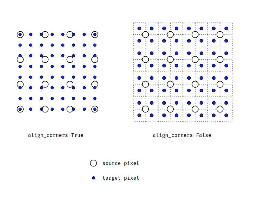
Figure 7: Upsampling alignments options extracted from [24].

• Complex Upsampling Upsampling layer for 2D inputs. The upsampling can be done using the nearest neighbor or bilinear interpolation. There are at least two possible ways to implement the upsampling method depending if the corners are aligned or not (see Figure 7). Our implementation does not align corners.

• Complex Transposed Convolution Sometimes called Deconvolution although it does not compute the inverse of a convolution [25].

• Complex Un-Pooling Inspired on the functioning of Max Un-pooling explained in Reference [26]. Max un-pooling technique receives the maxed locations of a previous Max Pooling layer and then expands an image by placing the input values on those locations and filling the rest with zeros as shown in Figure 8.

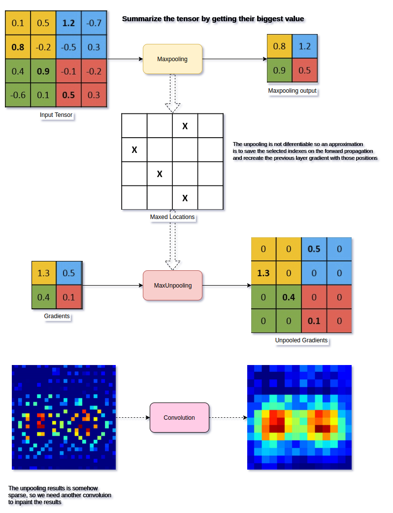
Figure 8: Max Unpooling graphical explanation extracted from [26].

Complex un-pooling locations are not forced to be the output of a max pooling layer. However, in order to use it, we implemented as well a layer class named ComplexMaxPooling2DWithArgmax which returns a tuple of tensors, the max pooling output and the maxed locations to be used as input of the un-pooling layer.

There are two main ways to use the unpooling layer, either by using the expected output shape or using the upsampling_factor parameter.

⬇

1from cvnn.layers import ComplexUnPooling2D, complex_input, ComplexMaxPooling2DWithArgmax

2import tensorflow as tf

3import numpy as np

4

5x = get_img() # Gets an image just for the example

6# Removes the batch size shape

7inputs = complex_input(shape=x.shape[1:])

8# Apply max-pooling and also get argmax

9max_pool_o, max_arg = ComplexMaxPooling2DWithArgmax(strides=1, data_format="channels_last", name="argmax")(inputs)

10# Applies the Unpooling

11outputs = ComplexUnPooling2D(x.shape[1:])([max_pool_o, max_arg])

12

13model = tf.keras.Model(inputs=inputs, outputs=outputs, name="pooling_model")

14model.summary()

15model(x)

It is possible to work with variable size images using a partially defined tensor, for example, shape=(None, None, 3). In this case, the second option (using upsampling_factor) is the only way to deal with them in the following manner.

⬇

1# Input is an unknown size RGB image

2inputs = complex_input(shape=(None, None, 3))

3max_pool_o, pool_argmax = ComplexMaxPooling2DWithArgmax(strides=1, data_format="channels_last", name="argmax")(inputs)

4unpool = ComplexUnPooling2D(upsampling_factor=2)([max_pool_o, pool_argmax])

5

6model = tf.keras.Model(inputs=inputs, outputs=outputs, name="pooling_model")

7model.summary()

8model(x)

All the discussed layers in this Section have a dtype parameter which defaults to tf.complex64, however, if tf.float32 or tf.float64 is used, the layer behaviour should be arithmetically equivalent to the corresponding Tensorflow layer, allowing for fast test and comparison. In some cases, for example, ComplexFlatten, this parameter has no effect as the layer can already deal with both complex- and real-valued input. Also, a method get_real_equivalent is implemented which returns a new layer object with a real-valued dtype and allows a output_multiplier parameter in order to re-dimension the real network if needed. This is used to obtain an equivalent real-valued network as described [27].

4 Complex Activation functions

One of the essential characteristics of CVNN is its activation functions, which should be non-linear and complex-valued. An activation function is usually chosen to be piece-wise smooth to facilitate the computation of the gradient. The complex domain widens the possibilities to design an activation function, but the probable more natural way would be to extend a real-valued activation function to the complex domain.

Our toolbox currently supports a wide range of complex-activation functions listed on act_dispatcher dictionary.

⬇

1act_dispatcher = {

2 ’linear’: linear,

3 # Complex input, real output

4 ’cast_to_real’: cast_to_real,

5 ’convert_to_real_with_abs’: convert_to_real_with_abs,

6 ’sigmoid_real’: sigmoid_real,

7 ’softmax_real_with_abs’: softmax_real_with_abs,

8 ’softmax_real_with_avg’: softmax_real_with_avg,

9 ’softmax_real_with_mult’: softmax_real_with_mult,

10 ’softmax_of_softmax_real_with_mult’: softmax_of_softmax_real_with_mult,

11 ’softmax_of_softmax_real_with_avg’: softmax_of_softmax_real_with_avg,

12 ’softmax_real_with_polar’: softmax_real_with_polar,

13 # Phasor networks

14 ’georgiou_cdbp’: georgiou_cdbp,

15 ’mvn_activation’: mvn_activation,

16 ’complex_signum’: complex_signum,

17 # Type A (cartesian)

18 ’cart_sigmoid’: cart_sigmoid,

19 ’cart_elu’: cart_elu,

20 ’cart_exponential’: cart_exponential,

21 ’cart_hard_sigmoid’: cart_hard_sigmoid,

22 ’cart_relu’: cart_relu,

23 ’cart_leaky_relu’: cart_leaky_relu,

24 ’cart_selu’: cart_selu,

25 ’cart_softplus’: cart_softplus,

26 ’cart_softsign’: cart_softsign,

27 ’cart_tanh’: cart_tanh,

28 ’cart_softmax’: cart_softmax,

29 # Type B (polar)

30 ’pol_tanh’: pol_tanh,

31 ’pol_sigmoid’: pol_sigmoid,

32 ’pol_selu’: pol_selu,

33 # Elementary Transcendental Functions (ETF)

34 ’etf_circular_tan’: etf_circular_tan,

35 ’etf_circular_sin’: etf_circular_sin,

36 ’etf_inv_circular_atan’: etf_inv_circular_atan,

37 ’etf_inv_circular_asin’: etf_inv_circular_asin,

38 ’etf_inv_circular_acos’: etf_inv_circular_acos,

39 ’etf_circular_tanh’: etf_circular_tanh,

40 ’etf_circular_sinh’: etf_circular_sinh,

41 ’etf_inv_circular_atanh’: etf_inv_circular_atanh,

42 ’etf_inv_circular_asinh’: etf_inv_circular_asinh,

43 # ReLU

44 ’modrelu’: modrelu,

45 ’crelu’: crelu,

46 ’zrelu’: zrelu,

47 ’complex_cardioid’: complex_cardioid

48}

Indeed, to implement an activation function, it will suffice to add it to the act_dispatcher dictionary to have full functionality.

In our published toolbox, there are two ways of using an activation function, either by using a string listed on act_dispatcher like

⬇

1ComplexDense(units=x, activation=’cart_sigmoid’)

or by using the function directly

⬇

1from cvnn.activations import cart_sigmoid

2

3ComplexDense(units=x, activation=cart_sigmoid)

This usage also support using tf.keras.layers.Activation to implement an activation function directly as an independent layer.

⬇

1 from cvnn.activations import cart_relu

2

3 layer = tf.keras.layers.Activation(’cart_relu’)

4 layer = tf.keras.layers.Activation(cart_relu)

Although complex activation functions used on CVNN are numerous [28, 29, 30], we will mainly focus on two types of activation functions that are an extension of the real-valued functions [31]:

• Type-A: $\sigma_{A}(z)=\sigma_{\mathrm{Re}}\left(\mathrm{Re}(z)\right)+i\,\sigma_{\mathrm{Im}}\left(\mathrm{Im}(z)\right)$,

• Type-B: $\sigma_{B}(z)=\sigma_{r}(|z|)\,\exp{\left(i\,\sigma_{\phi}(\arg(z))\right)}$,

where $\sigma_{\mathrm{Re}},\sigma_{\mathrm{Im}},\sigma_{r},\sigma_{\phi}$ are all real-valued functions. $\mathrm{Re}$ and $\mathrm{Im}$ operators are the real and imaginary parts of the input, respectively, and the $\arg$ operator gives the phase of the input. Note that in Type-A, the real and imaginary parts of an input go through nonlinear functions separately, and in Type-B, the magnitude and phase go through nonlinear functions separately.

The most popular activation functions, sigmoid, hyperbolic tangent (tanh)and Rectified Linear Unit (ReLU), are extensible using Type-A or Type-B approach. Although tanh is already defined on the complex domain for what, its transformation is probably less interesting.

Other complex-activation functions are supported by our toolbox including elementary transcentental functions (complex-valued-neural-networks.rtfd.io/en/latest/activations/etf.html) [32, 33] or phasor activation function (complex-valued-neural-networks.rtfd.io/en/latest/activations/mvn_activation.html) such as multi-valued neuron (MVN) activation function [34, 35] or Georgiou CDBP [36].

4.1 Complex Rectified Linear Unit (ReLU)

Normally, $\sigma_{\phi}$ is left as a linear mapping [31, 3]. Under this condition, using Rectified Linear Unit (ReLU)activation function for $\sigma_{r}$ has a limited interest since the latter makes $\sigma_{B}$ converge to a linear function, limiting Type-B ReLU usage. Nevertheless, ReLU has increased in popularity over the others as it has proved to learn several times faster than equivalents with saturating neurons [37]. Consequently, probably the most common complex-valued activation function is Type-A ReLU activation function more often defined as Complex-ReLU or $\mathbb{C}$ReLU [7, 38].

However, several other ReLU adaptations to the complex domain were defined throughout the bibliography as zReLU [39], defined as

$$\textrm{zReLU}(z)=\begin{cases}z&\textrm{if }0<\arg(z)<\pi/2\\ 0&\textrm{if otherwise}\end{cases}\,,$$ (35)

letting the output as the input only if both real and imaginary parts are positive. Another popular adaptation is modReLU [40], defined as

$$\textrm{modReLU}(z)=\begin{cases}\textrm{ReLU}\left(|z|+b\right)\displaystyle\frac{z}{|z|}&\textrm{if }|z|\geq b\\ 0&\textrm{if otherwise}\end{cases}\,,$$ (36)

where $b$ is an adaptable parameter defining a radius along which the output of the function is 0. This function provides a point-wise non-linearity that affects only the absolute value of a complex number. Another extension of ReLU, is the complex cardioid proposed by [41]

$$\sigma(z)=\frac{\left(1+\cos{(\arg(z))}\right)z}{2}\,.$$ (37)

This function maintains the phase information while attenuating the magnitude based on the phase itself.

These last three activation functions (cardioid, zReLU and modReLU) were analyzed and compared against each other in [28].

The discussed variants were implemented in the toolbox documented as usual in complex-valued-neural-networks.rtfd.io/en/latest/activations/relu.html.

4.2 Output layer activation function

The image domain of the output layer depends on the set of data labels. For classification tasks, real-valued integers or binary numbers are frequently used to label each class. For these cases, one option would be to cast the labels to the complex domain as done in [23], where a transformation is done to a label $c\in\mathbb{R}$ like $T:c\to c+i\,c$.

The second option is to use an activation function $\sigma:\mathbb{C}\to\mathbb{R}$ as the output layer. A popular real-valued activation used for classification tasks is the softmax function [42] (normalized exponential), which maps the magnitude to $[0,1]$, so the image domain is homogeneous to a probability. There are several options on how to transform this function to accept complex input and still have its image $\in[0;1]$. These options include either performing an average of the magnitudes $\sigma_{\mathrm{Re}},\sigma_{\mathrm{Im}}$ or $\sigma_{r},\sigma_{\phi}$, using only one of the magnitudes like $\sigma_{r}$ or apply the real-valued softmax to either the addition or multiplication of $\sigma_{\mathrm{Re}},\sigma_{\mathrm{Im}}$ or $\sigma_{r},\sigma_{\phi}$, between other options. Most of these variants are implemented in the library detailed in this Chapter and documented in complex-valued-neural-networks.rtfd.io/en/latest/activations/real_output.html.

5 Complex-compatible Loss functions

For CVNN s, the loss or cost function to minimize will have a real-valued output as one can not look for the minimum of two complex numbers. If the application is that of classification or semantic segmentation (as it is in all the cases of study of this work), there are a few options on what to do.

Some loss functions support this naturally. Reference [43] compares the performance of different type of complex input compatible loss functions. If the loss function to be used does not support complex-valued input, a popular option is to manage this through the output activation function as explained in the previous Section 4.2. However, a second option for non-complex-compatible loss functions such as categorical cross-entropy is to compare both the real and imaginary parts of the prediction independently with the labels and compute the loss function as an average of both results. Reference [38], for example, defines a loss function as the complex average cross-entropy as:

$$\mathcal{L}^{ACE}=\frac{1}{2}\left[\mathcal{L}^{CCE}\left(\mathrm{Re}{(y)},d\right)+\mathcal{L}^{CCE}\left(\mathrm{Im}{(y)},d\right)\right]\,,$$ (38)

where $\mathcal{L}^{ACE}$ is the complex average cross-entropy, $\mathcal{L}^{CCE}$ is the well-known categorical cross-entropy. $y$ is the network predicted output, and $d$ is the corresponding ground truth or desired output. For real-valued output $\mathcal{L}^{ACE}=\mathcal{L}^{CCE}$. This function was implemented in the published code alongside other variants, such as multiplying each class by weight for imbalanced classes or ignoring unlabeled data. All these versions are documented in complex-valued-neural-networks.rtfd.io/en/latest/losses.htm.

When the desired output is already complex-valued (regression tasks), more natural definitions can be used, such as proposed by [29], where the loss is defined as

$$\mathcal{L}=\frac{1}{2}\sum_{k}e_{k}\overline{e_{k}}\,,$$ (39)

where $e_{k}(y_{k},d_{k})$ is a complex error computation of $y_{k}$ and $d_{k}$ such as a subtraction.

6 Complex Batch Normalization

The complex Batch Normalization (BN)was adapted from the real-valued BN technique by Reference [7]. For normalizing a complex vector, we will treat the problem as a 2D vector instead of working on the complex domain so that $z=a+i\,b\in\mathbb{C}\longrightarrow\bm{x}=(a,b)\in\mathbb{R}^{2}$.

To normalize a complex variable, we need to compute

$$\bm{o}=\hat{\bm{\Sigma}}^{-\frac{1}{2}}(\bm{x}-\hat{\bm{\mu}})\,,$$ (40)

where $\bm{o}$ is the normalized output, $\hat{\bm{\mu}}$ is the mean estimate of $\mathbb{E}[\bm{x}]$, and $\hat{\bm{\Sigma}}\in\mathbb{R}^{2\times 2}$ is the estimated covariance matrix of $\bm{x}$ so that

$$\hat{\bm{\Sigma}}=\left[{\begin{array}[]{cc}\Sigma_{rr}&\Sigma_{ri}\\ \Sigma_{ir}&\Sigma_{ii}\\ \end{array}}\right]=\left[{\begin{array}[]{cc}\mathrm{Cov}(\mathrm{Re}(x)\mathrm{Re}(x))&\mathrm{Cov}(\mathrm{Re}(x)\mathrm{Im}(x))\\ \mathrm{Cov}(\mathrm{Im}(x)\mathrm{Re}(x))&\mathrm{Cov}(\mathrm{Im}(x)\mathrm{Im}(x))\\ \end{array}}\right]\,.$$ (41)

During the batch normalization layer initialization, two variables $\bm{\Sigma^{\prime}}\in\mathbb{R}^{2\times 2}$ (moving variance) and $\bm{\mu^{\prime}}\in\mathbb{R}^{2}$ (moving mean) are initialized. By default, $\bm{\Sigma^{\prime}}=\mathbf{I}/\sqrt{2}$ and $\bm{\mu}^{\prime}$ is initialized to zero.

During the training phase, $\hat{\bm{\Sigma}}$ and $\hat{\bm{\mu}}$ are computed on the innermost dimension of the training input batch (for multi-dimensional inputs where $z\in\mathbb{C}^{N}\to x\in\mathbb{R}^{N\times 2}$). The output of the layer is then computed as in Equation 40. The moving variance and moving mean are iteratively updated using the following rule:

$$\bm{\mu^{\prime}}_{k+1} =m\,\bm{\mu^{\prime}}_{k}+(1-m)\,\hat{\bm{\mu}}_{k}$$ (42)

$$\bm{\Sigma^{\prime}}_{k+1} =m\,\bm{\Sigma^{\prime}}_{k}+(1-m)\,\hat{\bm{\Sigma}}_{k}\,,$$ (43)

where $m$ is the momentum, a constant parameter set to $0.99$ by default.

During the inference phase, that is, for example, when performing a prediction, no variance nor average is computed. The output is directly calculated using the moving variance and moving average as

$$\hat{\bm{x}}=\bm{\Sigma^{\prime}}^{-\frac{1}{2}}(\bm{x}-\bm{\mu^{\prime}})\,.$$ (44)

Analogously to the real-valued batch normalization, it is possible to shift and scale the output by using the trainable parameters $\bm{\beta}$ and $\bm{\Gamma}$. In this case, the output $\bm{o}$ for both the training and prediction phase will be changed to $\hat{\bm{o}}=\bm{\Gamma}\,\bm{o}+\bm{\beta}$. By default, $\bm{\beta}$ is initialized to $(0,0)^{T}\in\mathbb{R}^{2}$ and

$$\bm{\Gamma}=\left({\begin{array}[]{cc}1/\sqrt{2}&0\\ 0&1/\sqrt{2}\\ \end{array}}\right)\,.$$ (45)

7 Complex Random Initialization

If we are to blindly apply any well-known random initialization algorithm to both real and imaginary parts of each trainable parameter independently, we might lose the special properties of the used initialization. This is the case, for example, for Glorot, also known as Xavier, initializer [44].

Assuming that:

• The input features have the same variance $\mathrm{Var}\left[X_{i}^{(0)}\right]\triangleq\mathrm{Var}\left[X^{(0)}\right],\forall i\in[|1;N_{0}|]$ and have zero mean (can be adjusted by the bias input).

• All the weights are statistically centered, and there is no correlation between real and imaginary parts.

• The weights at layer $l$ share the same variance $\mathrm{Var}\left[\omega_{i,j}^{(l)}\right]\triangleq\mathrm{Var}\left[\omega^{(l)}\right],\forall(i,j)\in[|1;N_{l+1}|]\times[|1;N_{l}|]$ and are statistically independent of the others layer weights and of inputs $X^{(0)}$.

• We are working on the linear part of the activation function. Therefore, $\sigma(z)\approx z$, which is the same as saying that $\sigma(z,\overline{z})\approx z$. The partial derivatives will then be

$$\begin{cases}\displaystyle\frac{\partial\sigma}{\partial z}\approx 1\\ \displaystyle\frac{\partial\sigma}{\partial\overline{z}}\approx 0\end{cases}$$ (46)

so that $\displaystyle\frac{\partial\sigma\left(V_{n}^{(l)}\right)}{\partial V_{n}^{(l)}}\approx 1$ and $\displaystyle\frac{\partial\overline{\sigma\left(V_{n}^{(l)}\right)}}{\partial V_{n}^{(l)}}\approx 0$, with $V_{n}^{(l)}$ defined in Section 2.3. This is an acceptable assumption when working with logistic sigmoid or tanh activation functions.

Using the notation of Section 2.3, for a dense feed-forward neural network with a bias initialized to zero (as is often the case), each neuron at hidden layer $l$ is expressed as

$$X_{n}^{(l)}\triangleq\sigma\left(V_{n}^{(l)}\right)=\sigma\left(\sum_{m=1}^{N_{l-1}}\omega^{(l)}_{nm}X_{m}^{(l-1)}\right),\forall n\in[|1;N_{l}|].$$ (47)

Since $\sigma$ is working on the linear part, from (47) we get that

$$\mathrm{Var}\left[X_{n}^{(l)}\right]=\mathrm{Var}\left[\sum_{m=1}^{N_{l-1}}\omega^{(l)}_{nm}X_{m}^{(l-1)}\right]\,,$$ (48)

where $X_{m}^{(l-1)}$ is a combination of $\omega^{(k)},1\leq k\leq l-1$ and $x^{(0)}$, so it is independent of $\omega^{(l)}$ which leads to

$$\mathrm{Var}\left[X_{n}^{(l)}\right]=\sum_{m=1}^{N_{l-1}}\mathrm{Var}\left[\omega^{(l)}_{nm}\right]\mathrm{Var}\left[X_{m}^{(l-1)}\right]\,,$$ (49)

As the weights share the same variance at each layer,

$$\mathrm{Var}\left[X_{n}^{(l)}\right] =\mathrm{Var}\left[\omega^{(l)}\right]\sum_{m=1}^{N_{l-1}}\mathrm{Var}\left[X_{m}^{(l-1)}\right]\,,$$

$$=\mathrm{Var}\left[\omega^{(l)}\right]\mathrm{Var}\left[\omega^{(l-1)}\right]\sum_{m=1}^{N_{l-1}}\sum_{p=1}^{N_{l-2}}\mathrm{Var}\left[X_{p}^{(l-2)}\right]\,,$$

$$=N_{l-1}\mathrm{Var}\left[\omega^{(l)}\right]\mathrm{Var}\left[\omega^{(l-1)}\right]\sum_{p=1}^{N_{l-2}}\mathrm{Var}\left[X_{p}^{(l-2)}\right]\,.$$ (50)

We can now obtain the variance of $X_{n}^{(l)}$ as a function of $x^{(0)}$ by applying Equation (50) recursively and assuming $X_{n}^{(0)},n=1,\ldots,N_{0}$ sharing the same variance,

$$\mathrm{Var}\left[X_{n}^{(l)}\right]=\mathrm{Var}\left[x^{(0)}\right]\prod_{m=1}^{l}N_{m-1}\mathrm{Var}\left[\omega^{(m)}\right]\,.$$ (51)

From a forward-propagation point of view, to keep a constant flow of information, then

$$\mathrm{Var}\left[X_{n}^{(l)}\right]=\mathrm{Var}\left[X_{n}^{(l^{\prime})}\right]\,,\forall 1\leq l<l^{\prime}\leq N$$ (52)

which implies that $\displaystyle N_{m-1}\mathrm{Var}\left[\omega^{(m)}\right]=1\,,\forall 1\leq m\leq N$.

On the other hand,

$$\frac{\partial\mathcal{L}}{\partial V_{n}^{(l)}} =\sum_{k=1}^{N_{l+1}}\frac{\partial\mathcal{L}}{\partial V_{k}^{(l+1)}}\frac{\partial V_{k}^{(l+1)}}{\partial X_{n}^{(l)}}\frac{\partial X_{n}^{(l)}}{\partial V_{n}^{(l)}}+\frac{\partial\mathcal{L}}{\partial\overline{V_{k}^{(l+1)}}}\frac{\partial\overline{V_{k}^{(l+1)}}}{\partial X_{n}^{(l)}}\frac{\partial X_{n}^{(l)}}{\partial V_{n}^{(l)}}+R\,,$$

$$=\sum_{k=1}^{N_{l+1}}\frac{\partial\mathcal{L}}{\partial V_{n}^{(l+1)}}\omega_{k,n}^{(l+1)}\,.$$ (53)

where R is the remaining terms depending on $\displaystyle\frac{\partial\overline{X_{n}^{(l)}}}{\partial V_{n}^{(l)}}$, which is assumed to be $0$ because the activation function is working in the linear regime at the initialization, i.e. $\displaystyle\frac{\partial X_{n}^{(l)}}{\partial V_{n}^{(l)}}\approx 1$ and $\displaystyle\frac{\partial\overline{X_{n}^{(l)}}}{\partial V_{n}^{(l)}}\approx 0$. The last equality is held since $\displaystyle\frac{\partial V_{k}^{(l+1)}}{\partial X_{n}^{(l)}}=\omega_{k,n}^{(l+1)}$ and $\frac{\partial V_{k}^{(l+1)}}{\partial\overline{X_{n}^{(l)}}}=0$ (see (33) in Appendix for the general case).

Assuming the loss variation w.r.t. the output neuron is statistically independent of any weights at any layers, then we can deduce recursively from (53),

$$\mathrm{Var}\left[\frac{\partial\mathcal{L}}{\partial V_{n}^{(l)}}\right]=\mathrm{Var}\left[\frac{\partial\mathcal{L}}{\partial V_{n}^{(L)}}\right]\prod_{m=l+1}^{L}N_{m}\mathrm{Var}\left[\omega^{(m)}\right]\,.$$ (54)

From a back-propagation point of view, we want to keep a constant learning flow:

$$\mathrm{Var}\left[\frac{\partial\mathcal{L}}{\partial V_{n}^{(l)}}\right]=\mathrm{Var}\left[\frac{\partial\mathcal{L}}{\partial V_{n}^{(l^{\prime})}}\right],\,\forall 1\leq l<l^{\prime}\leq N,$$ (55)

which implies $N_{m}\mathrm{Var}\left[\omega^{(m)}\right]=1,\,\forall 1\leq m\leq N$.

Conditions (52) and (55) are not possible to be satisfied at the same time (unless $N_{l}=N_{l+1}$, $\forall 1\leq l<N$ , meaning all layers should have the same width) for what Reference [44] proposes the following trade-of

$$\mathrm{Var}\left[\omega^{(l)}\right]=\frac{2}{N_{l}+N_{l+1}}\,,\forall 1\leq l<N\,.$$ (56)

If the weight initialization is a uniform distribution $\sim U$, for the real-valued case, the initialization that has the variance stated on Equation 56 is:

$$\omega^{(l)}\sim U\left[-\frac{\sqrt{6}}{\sqrt{N_{l}+N_{l+1}}},\frac{\sqrt{6}}{\sqrt{N_{l}+N_{l+1}}}\right]\,.$$ (57)

For a complex variable with no correlation between real and imaginary parts, the variance is defined as:

$$\mathrm{Var}\left[\omega^{(l)}\right]=\mathrm{Var}\left[\mathrm{Re}\left(\omega^{(l)}\right)\right]+\mathrm{Var}\left[\mathrm{Im}\left(\omega^{(l)}\right)\right]\,,$$ (58)

it is therefore logical to choose both variances $\mathrm{Var}\left[\mathrm{Re}\left(\omega^{(l)}\right)\right]$ and $\mathrm{Var}\left[\mathrm{Im}\left(\omega^{(l)}\right)\right]$ to be equal:

$$\mathrm{Var}\left[\mathrm{Re}\left(\omega^{(l)}\right)\right]=\mathrm{Var}\left[\mathrm{Im}\left(\omega^{(l)}\right)\right]=\frac{1}{N_{l}+N_{l+1}}\,.$$ (59)

With this definition, the complex variable could be initialized as:

$$\mathrm{Re}\left(\omega^{(l)}\right)=\mathrm{Im}\left(\omega^{(l)}\right)\sim U\left[-\frac{\sqrt{3}}{\sqrt{N_{l}+N_{l+1}}},\frac{\sqrt{3}}{\sqrt{N_{l}+N_{l+1}}}\right]\,.$$ (60)

By comparing (57) with (60) it is concluded that to correctly implement a Glorot initialization, one should divide the real and imaginary part of the complex weight by $\sqrt{2}$.

It is also possible to define the initialization technique from a polar perspective. The variance definition is

$$\mathrm{Var}\left[\omega^{(l)}\right]=E\left[\left|\omega^{(l)}-E\left[\omega^{(l)}\right]^{2}\right|\right]=E\left[\left|\omega^{(l)}\right|^{2}\right]+\left|E\left[\omega^{(l)}\right]\right|^{2}\,.$$ (61)

By choosing the phase to be a uniform distribution between $0$ and $2\pi$ and knowing the absolute is always positive, then $E\left[\omega^{(l)}\right]=0$ and Equation 61 can be simplified to:

$$\mathrm{Var}\left[\omega^{(l)}\right]=E\left[\left|\omega^{(l)}\right|^{2}\right]\,.$$ (62)

It will therefore suffice to choose any random initialization, such as, for example, a Rayleigh distribution [45], for $\left|\omega^{(l)}\right|=\rho\in\mathbb{R}_{0}^{+}$ so that

$$E\left[\rho^{2}\right]=\frac{2}{N_{l}+N_{l+1}}\,.$$ (63)

7.1 Impact of complex-initialization equation application

A simulation was done for a complex multi-layer network with four hidden layers of size 128, 64, 32 and 16, respectively, with a logistic sigmoid activation function to test the impact of this constant division by $\sqrt{2}$ on a signal classification task. One-hundred and fifty epochs were done with one thousand runs of each model to obtain statistical results.

The task consisted in classifying different signals used in radar applications. Temporal and time-frequency representations of each signal are shown in Figures 9 and 10 respectively. The generated signals are

• Sweep or chirp signal. These are signals whose frequency changes over time. These types of signals are commonly applied to radar. The chirp-generated signals were of two types, either linear chirp, where the frequency changed linearly over time or S-shaped, whose frequency variation gets faster at both the beginning and the end, forming an S-shaped spectrum as can be seen in Figure 10.

• Phase-Shift Keying (PSK)modulated signals, a digital modulation process that conveys data by changing the phase of a constant frequency reference signal. These signals were BPSK (2-phase states) and QPSK (4-phase states)

• Quadrature Amplitude Modulation (QAM)signals, which are a combination of amplitude and phase modulation. These signals were 16QAM (4 phase and amplitude states) and 64QAM (8 phase and amplitude states).

A noise signal (null), without any signal of interest, was also used, making a total of 7 different classes.

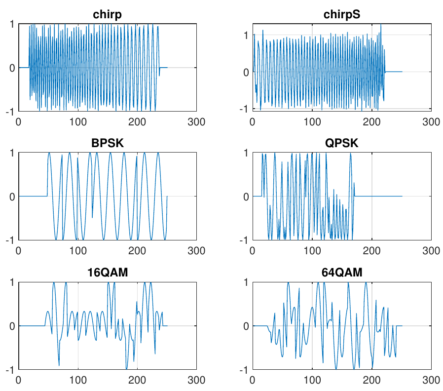
Figure 9: Temporal amplitude examples of used signals [46].

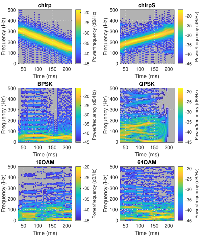
Figure 10: Spectrogram examples of used signals [46].

Instead of using measured signals, and with the goal of facilitating the studies, the signals were randomly generated, which also allowed having the ground truth. These generated signals had the following properties:

• 256 samples per signal

• Peak-to-peak amplitude of 1

• Chirp signals with frequencies from 0.05 to 0.45 times the sample frequency

• Number of moments between 8 and 64 for the codes BPSK, QPSK, 16QAM and 64QAM

Thermal noise was added to each signal and was transformed to the complex domain using the Hilbert Transform, a popular transformation in signal processing applications [47], which provides an analytic mapping of a real-valued function to the complex plane.

The Hilbert transpose has its origins in 1902 when the English mathematician Godfrey Harold Hardy (1877 – 1947) introduced a transformation that consisted in the convolution of a real function $f(s)$ [48, 49], with the Cauchy kernel $\displaystyle 1/\pi(t-s)$ which, being an improper integral, must be defined in terms of its principal value (p.v.) [50],

$$\mathcal{H}(f)(t) =\frac{1}{\pi}\text{p.v.}\int_{-\infty}^{+\infty}\frac{f(s)}{t-s}ds =\frac{1}{\pi}\lim_{\varepsilon\to 0}\int_{\varepsilon}^{+\infty}\frac{f(t-s)-f(t+s)}{s}ds\,.$$ (64)

One of the most important properties of this transformation is that its repeated application allows for the recovery of the original function, with only a change of sign, that is,

$$g(t)=\mathcal{H}(f)(t)\Leftrightarrow f(t)=-\mathcal{H}(g)(t)\,.$$ (65)

The functions $f$ and $g$ that satisfy this relation are called Hilbert transform pairs, in honor of David Hilbert, who first studied them in 1904 [51]. In fact, it is for this reason that in 1924 [52, 53], Hardy graciously proposed calling transformation (64) as Hilbert Transform.

Some examples of Hilbert transform pairs are shown in Table 1.

$f(t)$	$g(t)=\mathcal{H}(f)(t)$
$\sin(t)$	$\cos(t)$
$1/\left(t^{2}+1\right)$	$t/\left(t^{2}+1\right)$
$\sin(t)/t$	$\left[1-\cos(t)\right]/t$
$\delta(t)$	$1/\pi t$

Table 1: Examples of Hilbert transform pairs

Considering the definition of the Fourier transform of an absolutely integrable real function $f(s)$,

$$\mathcal{F}(f)(t)\,.$$ (66)

It can be shown that [50]

$$\mathcal{F}\left(\mathcal{H}(f)(t)\right)=-i\,\text{sgn}(t)\mathcal{F}(f)(t)\,.$$ (67)

This relation provides an effective way to evaluate the Hilbert transform

$$\mathcal{H}(f)=-i\,\mathcal{F}^{-1}\left[\text{sgn}\mathcal{F}(f)(t)\right]\,,$$ (68)

avoiding the issue of dealing with the singular structure of the Cauchy kernel.

One of the most important properties of the Hilbert transform, at least in reference to this thesis, is that the real and imaginary parts of a function $h(z)$ that is analytic in the upper half of the complex plane are Hilbert transform pairs. That is to say that

$$\mathrm{Im}(h)=\mathcal{H}(\mathrm{Re}(h))\,.$$ (69)

In this way, the Hilbert transform provides a simple method of performing the analytic continuation to the complex plane of a real function $f(x)$ defined on the real axis, defining $h(z)=f(z)+i\,g(z)$ with $g(z)=\mathcal{H}(f)$. This property of the Hilbert transform was independently discovered by Ralph Kronig [54] (1904 – 1995), and Hans Kramers [55] (1894 - 1952) in 1926 in relation to the response function of physical systems, known as the Kramers-Kronig relation. At the same time, it began to be used in circuit analysis [56] in relation to the real and imaginary parts of the complex impedance. Through the work of pioneers such as the Nobel prize winner Dennis Gabor [57] (1900 – 1979), its application in modern signal processing is wide and varied [47].

The real and imaginary weights where initialized as described in (57) (The definition for real-valued weights, which is equivalent to multiplying the limits of Equation 60 by $\sqrt{2}$) and (60) (the original case for complex-valued weights) to compare them. An initialization that divided the limits of Equation 60 by two was also used to assert that smaller values will not produce a superior result either.

Figure 11: Comparison of Glorot Uniform initialization scaled by different values.

The results shown in Figure 11 prove the importance of the correct adaptation of Glorot initialization to complex numbers and how failing to do so will impact its performance negatively.

7.2 Experiment on different trade-offs

Complex numbers enable choosing different trade-offs than the one chosen by [44] (Equation 56), for example, the following trade-off can also be chosen:

$$\mathrm{Var}\left[\mathrm{Re}\left(\omega^{(l)}\right)\right]=\frac{1}{2N_{l}}\,,$$ (70)

$$\mathrm{Var}\left[\mathrm{Im}\left(\omega^{(l)}\right)\right]=\frac{1}{2N_{l+1}}\;,$$

between other options.

In a similar manner, as we did with Glorot (Xavier) initialization, the He weight initialization described in [58] can be deduced for complex numbers. the same dataset as the one used in the experiment of Figure 11 was done using Glorot Uniform ($GU$), Glorot Normal ($GN$), He Normal ($HN$), He Uniform ($HU$), and Glorot Uniform using the trade-off defined in (70) ($GU_{C}$).

Figure 12: Initialization Technique Comparison

The results of Figure 12 show that the difference between using a normal or uniform distribution is negligible but that Glorot clearly outperforms He initialization. This is to be expected when using sigmoid activation function because He initialization was designed for ReLU activation functions. On the other hand, the trade-off proposed in (70) actually achieves lower performances than the one proposed in [44] for what it was not implemented in the cvnn toolbox, however, it is possible this results is only specific to this dataset and for what further research could be done with this trade-off variant. All the other initialization techniques are documented in complex-valued-neural-networks.rtfd.io/en/latest/initializers.html and implemented as previously described. They can be used in standalone mode as follows

⬇

1import cvnn

2initializer = cvnn.initializers.GlorotUniform()

3values = initializer(shape=(2, 2))

4# Returns a complex Glorot Uniform tensor of shape (2, 2)

or inside a layer using an initializer object like

⬇

1import cvnn

2initializer = cvnn.initializers.ComplexGlorotUniform()

3layer = cvnn.layers.Dense(input_size=23, output_size=45, weight_initializer=initializer)

or as a string listed within init_dispatcher like

⬇

1import cvnn

2

3layer = cvnn.layers.Dense(input_size=23, output_size=45, weight_initializer="ComplexGlorotUniform")

with init_dispatcher being

⬇

1init_dispatcher = {

2 "ComplexGlorotUniform": ComplexGlorotUniform,

3 "ComplexGlorotNormal": ComplexGlorotNormal,

4 "ComplexHeUniform": ComplexHeUniform,

5 "ComplexHeNormal": ComplexHeNormal

6}

8 Performance on real-valued data

Using the same signals of previous Sections, some experiments were perform comparing Complex-Valued MultiLayer Perceptron (CV-MLP)against a Real-Valued MultiLayer Perceptron (RV-MLP). 16000 Chirp signals were created, 8000 linear and 8000 S-shaped. $80\%$ was used for training, $10\%$ for validation and the remaining $10\%$ for testing. Two models (one CV-MLP and one RV-MLP) were designed and dimensioned as shown in Table 2.

	CV-MLP	RV-MLP
input size	256	512
hidden layers activation	Type-A Selu	Selu
$1^{\text{st}}$ hidden layer size	25	50
$2^{\text{nd}}$ hidden layer size	10	20
output activation	modulo softmax	modulo softmax
output size	7	7

Table 2: Design of MLP models

We used SGD as weight optimization and $50\%$ dropout for both models. We performed 2000 iterations (1000 for each model) with 2000 epochs each.

Figure 13 shows the mean loss per epoch of both training and validation set for CV-MLP (Figure 13(a)) and RV-MLP (Figure 13(b)). The Figures show that CV-MLP presents less overfitting than the real-valued model.

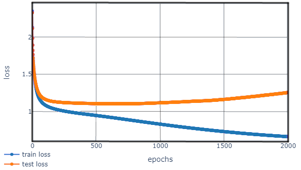
((a)) CV-MLP

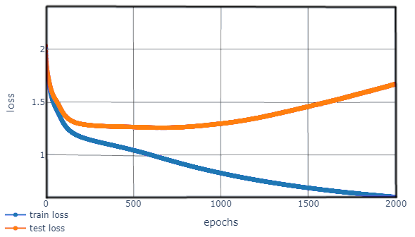
((b)) RV-MLP

Figure 13: Mean loss evolution per epoch.

A histogram of both models’ accuracy and loss values on the test set was plotted and can be seen in Figure 14. It is clear that CV-MLP outperforms RV-MLP classification accuracy with around $4\%$ higher accuracy. Regarding the loss, RV-MLP obtained higher variance.

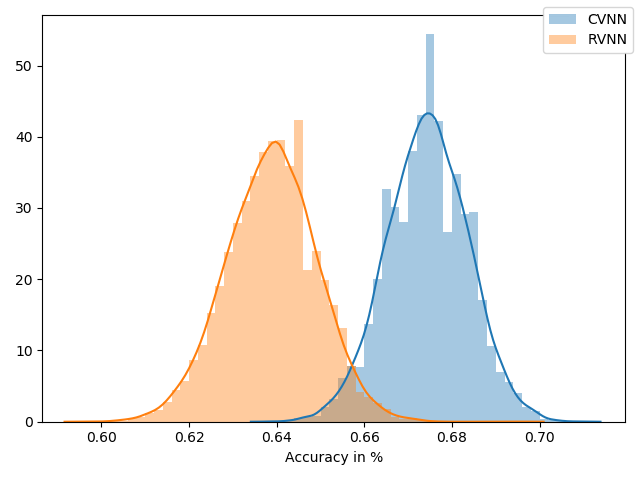
((a)) Accuracy

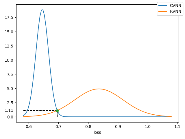
((b)) Loss

Figure 14: Test set histogram metrics for binary classification on Chirp signals.

Finally, the simulations were performed for all seven signals obtaining similar results as before. This time, accuracy results have a higher difference with CVNN results not intersecting with the RVNN results. Again, RV-MLP had higher loss variance.

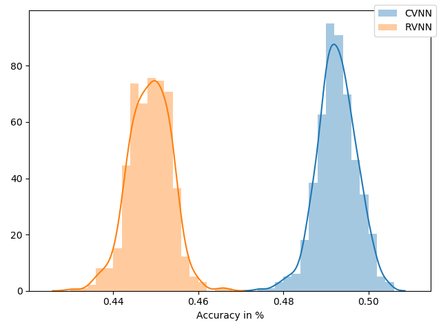
((a)) Accuracy

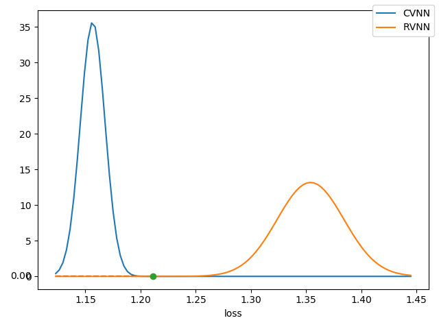
((b)) Loss

Figure 15: Test set histogram metrics for multi-class classification for all 7 signals.

8.1 Discussion

It is important to note that these networks were not optimized. The main issue is the softmax activation function used on the absolute value of the complex output. Although it is not generally used like this, in CVNN, it might be acceptable. However, for a RVNN, this is unconventional and penalizes their performance greatly. Furthermore, both models are not equivalent, as described in Reference [27], resulting in RVNN having a higher capacity, which may increase their performance but also may result in more overfitting.

For all these reasons, the simulations must be revised. However, if the general conclusions stand, this might indicate that CVNN can outperform RVNN even for real-valued applications when using an appropriate transformation such as the Hilbert transform.

9 Conclusion

In this paper, described in detail each adaptation from conventional real-valued neural networks to the complex domain in order to be able to implement Complex-Valued Neural Network s. Each aspect was revised, and the appropriate mathematics was developed. With this work it should be possible to understand and implement from a basic Complex-Valued MultiLayer Perceptron to a Complex-Valued Convolutional Neural Network and even Complex-Valued Fully Convolutional Neural Network or Complex-Valued U-Network (CV-UNET).

We also detail the implementation of the published library, with examples of how to use the code and with reference to the documentation to be used if needed. We showed that the library had great success in the community through its increasing popularity.

We performed simulations that verified the adaptation of the initialization technique and showed that correctly implementing this initialization is crucial for obtaining a good performance.

Finally, we show that CVNN s might be of interest even for real data by using the Hilbert transformation contrary to the work of [5]. The classification improved around $4\%$ when using a complex network over a real one. However, these last results should be revised as the models were not equivalent, and RVNN might have been overly penalized.

Appendix A Complex Identities

For further reading and properties of complex numbers, see Reference [59].

Definition A.1 (Hermitian transpose).

Given $\bm{A}\in\mathbb{C}^{n\times m},m,n\in\mathbb{N}^{+}$. The Hermitian transpose of a matrix is defined as:

$$\bm{A}^{H}=\overline{\bm{A}^{T}}\,.$$ (71)

The upper line on $\overline{A}$ refers to the conjugate value of a complex number, that is, a number with an equally real part and an imaginary part equal in magnitude but opposite in sign.

Definition A.2 (differential rule).

$$\partial f=\frac{\partial f}{\partial z}\partial z+\frac{\partial f}{\partial\overline{z}}\partial\overline{z}\,.$$ (72)

Definition A.3 (conjugation rule).

$$\overline{\left(\frac{\partial f}{\partial z}\right)} =\frac{\partial\overline{f}}{\partial\overline{z}}\,,$$ (73)

$$\overline{\left(\frac{\partial f}{\partial\overline{z}}\right)} =\overline{\frac{\partial f}{\partial z}}\,.$$

When $f:\mathbb{C}\longrightarrow\mathbb{R}$ the expression can be simplified as:

$$\overline{\left(\frac{\partial f}{\partial z}\right)} =\frac{\partial f}{\partial\overline{z}}$$ (74)

$$\overline{\left(\frac{\partial f}{\partial\overline{z}}\right)} =\frac{\partial f}{\partial z}\,.$$

Theorem A.1.

Given $f(z):\mathbb{C}\longrightarrow\mathbb{C},z=x+i\,y\Rightarrow\exists u,v:\mathbb{R}^{2}\longrightarrow\mathbb{R}$ such that $f(z)=u(x,y)+i\,v(x,y)$

A.1 Complex differentiation rules

Given $f,g:\mathbb{C}\longrightarrow\mathbb{C}$ and $c\in\mathbb{C}$:

$$(f+g)^{\prime}(z_{0}) =f^{\prime}(z_{0})+g^{\prime}(z_{0})\,,$$ (75)

$$(f\,g)^{\prime}(z_{0}) =f^{\prime}(z_{0})\,g(z_{0})+f(z_{0})\,g^{\prime}(z_{0})\,,$$

$$\left(\frac{f}{g}\right)^{\prime}(z_{0}) =\frac{f^{\prime}(z_{0})\,g(z_{0})-f(z_{0})\,g^{\prime}(z_{0})}{g^{2}(z_{0})}, g(z_{0})\neq 0\,,$$

$$(c\,f)^{\prime}(z_{0}) =c\,f^{\prime}(z_{0})\,.$$

A.2 Properties of the conjugate

Given $z,w\in\mathbb{C}$:

$$\overline{z\pm w} =\overline{z}\pm\overline{w}\,,$$ (76)

$$\overline{z\,w} =\overline{z}\,\overline{w}\,,$$

$$\overline{\left(\frac{z}{w}\right)} =\frac{\overline{z}}{\overline{w}}\,,$$

$$\overline{z^{n}} =\overline{z}^{n},\forall n\in\mathbb{C}\,,$$

$$|z|^{2} =z\,\overline{z}\,,$$

$$\overline{z}\,z =z\,\overline{z}\,,$$

$$\overline{\overline{z}} =z\text{ (involution)}\,,$$

$$\overline{z} =z\Leftrightarrow z\in\mathbb{R}\,,$$

$$z^{-1} =\frac{\overline{z}}{|z|^{2}},\forall z\neq 0\,.$$

A.3 Holomorphic Function

An holomorphic function is a complex-valued function of one or more complex variables that is, at every point of its domain, complex differentiable in a neighborhood of the point. This condition implies an holomorphic function is Class $C^{\infty}$ (analytic).

Definition A.4.

Given a complex function $f:\mathbb{C}\longrightarrow\mathbb{C}$ at a point $z_{0}$ of an open subset $\Omega\subset\mathbb{C}$ is complex-differentiable if exists a limit such as:

$$f^{\prime}(z_{0})=\lim_{z\to z_{0}}\frac{f(z)-f(z_{0})}{z-z_{0}}\,.$$ (77)

As stated before, if a function is complex-differentiable at all points of $\Omega$ it is called holomorphic [5]. The relationship between real differentiability and complex differentiability is stated on the Cauchy-Riemann equations

Theorem A.2 (Cauchy-Riemann equations).

Given $f(x+i\,y)=u(x,y)+i\,v(x,y)$ where $u,v:\mathbb{R}^{2}\longrightarrow\mathbb{R}$ real-differentiable functions, $f$ is complex-differentiable if satisfies:

$$\frac{\partial u}{\partial x} =\frac{\partial v}{\partial y}\,,$$ (78)

$$-\frac{\partial u}{\partial y} =\frac{\partial v}{\partial x}\,.$$

Proof.

Given $f:\mathbb{C}\longrightarrow\mathbb{C}$:

$$f(x+iy)=u(x,y)+i\,v(x,y)\,,$$ (79)

with $u,v:\mathbb{R}\longrightarrow\mathbb{R}$ real-differentiable functions.

For $f$ to be complex-differentiable, then:

$$f^{\prime}(z)=\lim_{\Delta x\to 0}\frac{f(z+\Delta x)-f(z)}{\Delta x}=\lim_{i\Delta y\to 0}\frac{f(z+i\,\Delta y)-f(z)}{i\,\Delta y}\,.$$ (80)

Replacing (80) with (79) and doing some algebra:

$$f^{\prime}(z)=\frac{\partial u}{\partial x}+i\,\frac{\partial v}{\partial x}=\frac{\partial v}{\partial y}-i\,\frac{\partial u}{\partial y}\,.$$ (81)

By comparing real and imaginary parts from the latest function, the
Cauchy-Riemann equations are evident. ∎

A.4 Chain Rule

Theorem A.3 (real multivariate chain rule with complex variable).

Given $f:\mathbb{R}^{2}\longrightarrow\mathbb{R},z\in\mathbb{C}$ and $x(z),y(z):\mathbb{C}\longrightarrow\mathbb{R}$

$$\frac{\partial f}{\partial z}=\frac{\partial f}{\partial x}\frac{\partial x}{\partial z}+\frac{\partial f}{\partial y}\frac{\partial y}{\partial z}\,.$$ (82)

This chain rule is analogous to that of the multivariate chain rule with real values. The need for stating this case arises from a demonstration that will be done for Theorem 87.

Theorem A.4 (complex chain rule over real and imaginary part).

Given $f:\mathbb{C}\longrightarrow\mathbb{C},z\in\mathbb{C}$ and $x(z),y(z):\mathbb{C}\longrightarrow\mathbb{R}$

$$\frac{\partial f}{\partial z}=\frac{\partial f}{\partial x}\frac{\partial x}{\partial z}+\frac{\partial f}{\partial y}\frac{\partial y}{\partial z}\,.$$ (83)

Proof.

By using theorem A.1, we can write $f=u+i\,v$ so that:

$$\frac{\partial f}{\partial z}=\frac{\partial u}{\partial z}+i\,\frac{\partial v}{\partial z}\,.$$ (84)

Using theorem A.3 we can apply the chain rule with $u$ and $v$:

$$\frac{\partial f}{\partial z}=\left[\frac{\partial u}{\partial x}\frac{\partial x}{\partial z}+\frac{\partial u}{\partial y}\frac{\partial y}{\partial z}\right]+i\left[\frac{\partial v}{\partial x}\frac{\partial x}{\partial z}+\frac{\partial v}{\partial y}\frac{\partial y}{\partial z}\right]\,.$$ (85)

Rearranging the terms leads to:

$$\frac{\partial f}{\partial z} =\left[\frac{\partial u}{\partial x}\frac{\partial x}{\partial z}+i\,\frac{\partial v}{\partial x}\frac{\partial x}{\partial z}\right]+\left[\frac{\partial u}{\partial y}\frac{\partial y}{\partial z}+i\,\frac{\partial v}{\partial y}\frac{\partial y}{\partial z}\right]\,,$$ (86)

$$=\left[\frac{\partial u}{\partial x}+i\,\frac{\partial v}{\partial x}\right]\frac{\partial x}{\partial z}+\left[\frac{\partial u}{\partial y}+i\,\frac{\partial v}{\partial y}\right]\frac{\partial y}{\partial z}\,,$$

$$=\left[\frac{\partial u+i\,\partial v}{\partial x}\right]\frac{\partial x}{\partial z}+\left[\frac{\partial u+i\,\partial v}{\partial y}\right]\frac{\partial y}{\partial z}\,,$$

$$=\left[\frac{\partial(u+i\,v)}{\partial x}\right]\frac{\partial x}{\partial z}+\left[\frac{\partial(u+i\,v)}{\partial y}\right]\frac{\partial y}{\partial z}\,,$$

$$=\frac{\partial f}{\partial x}\frac{\partial x}{\partial z}+\frac{\partial f}{\partial y}\frac{\partial y}{\partial z}\,.$$

∎

Corollary A.4.1.

See that the proof of Theorem A.3 is indistinct weather $z\in\mathbb{C}$ or $z\in\mathbb{R}$, so that both (A.3) and (A.4) are also valid for $z\in\mathbb{R}$

Definition A.5 (complex chain rule).

Given $h,g:\mathbb{C}\longrightarrow\mathbb{C},z\in\mathbb{C}$. The chain rule in complex numbers is now given by:

$$\frac{\partial h(g)}{\partial z} =\frac{\partial h}{\partial g}\frac{\partial g}{\partial z}+\frac{\partial h}{\partial\overline{g}}\frac{\partial\overline{g}}{\partial z}$$ (87)

$$\frac{\partial h(g)}{\partial\overline{z}} =\frac{\partial h}{\partial g}\frac{\partial g}{\partial\overline{z}}+\frac{\partial h}{\partial\overline{g}}\frac{\partial\overline{g}}{\partial\overline{z}}\,.$$

Proof.

As we make no assumption of $h$ or $g$ being holomorphic, we will use Wirtinger calculus (10) (having in mind that holomorphic functions are special cases of the later):

$$\frac{\partial\left(f\circ g\right)}{\partial z}=\frac{1}{2}\left(\frac{\partial\left(f\circ g\right)}{\partial z_{\mathrm{Re}{}}}-i\,\frac{\partial\left(f\circ g\right)}{\partial z_{\mathrm{Im}{}}}\right)\,.$$ (88)

Using (A.4.1):

$$\frac{\partial\left(f\circ g\right)}{\partial z} =\frac{1}{2}\left(\left(\frac{\partial f}{\partial g_{\mathrm{Re}{}}}\frac{\partial g_{\mathrm{Re}{}}}{\partial z_{\mathrm{Re}{}}}+\frac{\partial f}{\partial g_{\mathrm{Im}{}}}\frac{\partial g_{\mathrm{Im}{}}}{\partial z_{\mathrm{Re}{}}}\right)-i\,\left(\frac{\partial f}{\partial g_{\mathrm{Re}{}}}\frac{\partial g_{\mathrm{Re}{}}}{\partial z_{\mathrm{Im}{}}}+\frac{\partial f}{\partial g_{\mathrm{Im}{}}}\frac{\partial g_{\mathrm{Im}{}}}{\partial z_{\mathrm{Im}{}}}\right)\right)\,,$$ (89)

$$\begin{aligned} &=\frac{1}{4}\left(\frac{\partial f}{\partial g_{\mathrm{Re}{}}}\frac{\partial(g+\overline{g})}{\partial z_{\mathrm{Re}{}}}-i\,\frac{\partial f}{\partial g_{\mathrm{Im}{}}}\frac{\partial(g-\overline{g})}{\partial z_{\mathrm{Re}{}}}\right)\\ &\qquad\qquad-i\,\frac{1}{4}\left(\frac{\partial f}{\partial g_{\mathrm{Re}{}}}\frac{\partial(g+\overline{g})}{\partial z_{\mathrm{Im}{}}}-i\,\frac{\partial f}{\partial g_{\mathrm{Im}{}}}\frac{\partial(g-\overline{g})}{\partial z_{\mathrm{Im}{}}}\right)\end{aligned}$$ (90)

$$\begin{aligned} &=\frac{1}{4}\frac{\partial f}{\partial g_{\mathrm{Re}{}}}\left(\frac{\partial(g+\overline{g})}{\partial z_{\mathrm{Re}{}}}-i\,\frac{\partial(g+\overline{g})}{\partial z_{\mathrm{Im}{}}}\right)\\ &\qquad\qquad-\frac{1}{4}\frac{\partial f}{\partial g_{\mathrm{Im}{}}}\left(i\,\frac{\partial(g-\overline{g})}{\partial z_{\mathrm{Re}{}}}+\frac{\partial(g-\overline{g})}{\partial z_{\mathrm{Im}{}}}\right)\,.\end{aligned}$$ (91)

Using Wirtinger calculus definition again (Equation 10):

$$\frac{\partial\left(f\circ g\right)}{\partial z}=\frac{1}{2}\left(\frac{\partial f}{\partial g_{\mathrm{Re}{}}}\frac{\partial(g+\overline{g})}{\partial z}-i\frac{\partial f}{\partial g_{\mathrm{Im}{}}}\frac{\partial(g-\overline{g})}{\partial z}\right)\,.$$ (92)

Using (2.4.1):

$$\frac{\partial\left(f\circ g\right)}{\partial z} =\frac{1}{2}\left(\left(\frac{\partial f}{\partial g}+\frac{\partial f}{\partial\overline{g}}\right)\frac{\partial(g+\overline{g})}{\partial z}+\left(\frac{\partial f}{\partial g}-\frac{\partial f}{\partial\overline{g}}\right)\frac{\partial(g-\overline{g})}{\partial z}\right)\,,$$ (93)

$$=\frac{1}{2}\left(\frac{\partial f}{\partial g}\left(\frac{\partial(g+\overline{g})}{\partial z}+\frac{\partial(g-\overline{g})}{\partial z}\right)+\frac{\partial f}{\partial\overline{g}}\left(\frac{\partial(g+\overline{g})}{\partial z}-\frac{\partial(g-\overline{g})}{\partial z}\right)\right)\,,$$

$$=\frac{1}{2}\left(\frac{\partial f}{\partial g}\left(\frac{\partial(g+\overline{g})+\partial(g-\overline{g})}{\partial z}\right)+\frac{\partial f}{\partial\overline{g}}\left(\frac{\partial(g+\overline{g})-\partial(g-\overline{g})}{\partial z}\right)\right)\,,$$

$$=\frac{1}{2}\left(\frac{\partial f}{\partial g}\left(\frac{\partial(g+\overline{g}+g-\overline{g})}{\partial z}\right)+\frac{\partial f}{\partial\overline{g}}\left(\frac{\partial(g+\overline{g}-g+\overline{g})}{\partial z}\right)\right)\,,$$

$$=\left(\frac{\partial f}{\partial g}\frac{\partial g}{\partial z}+\frac{\partial f}{\partial\overline{g}}\frac{\partial\overline{g}}{\partial z}\right)\,.$$

∎

Appendix B Real Valued Backpropagation

To learn how to optimize the weight of $\omega^{(l)}_{ij}$, it is necessary to find the partial derivative of the loss function for a given weight. We will use the chain rule as follows:

$$\frac{\partial\mathcal{L}}{\partial\omega^{(l)}_{ij}}=\sum_{n=1}^{N_{L}}\frac{\partial e_{n}}{\partial X_{n}^{(L)}}\frac{\partial X_{n}^{(L)}}{\partial V_{n}^{(L)}}\frac{\partial V_{n}^{(L)}}{\partial\omega^{(l)}_{ij}}\,.$$ (94)

Given these three terms inside the addition, we could find the value we are looking for. The first two partial derivatives are trivial as $\partial e_{n}(d_{n},y_{n})/\partial y_{n}$ exists and is no zero and $\partial X_{n}^{(L)}/\partial V_{n}^{(L)}$ is the derivate of $\sigma$.

With regard to $\partial V_{n}^{(L)}/\partial\omega^{(l)}_{ij}$, when the layer is the same for both values ($l=L$), the definition is trivial and the following result is obtained:

$$\frac{\partial V_{i}^{(l)}}{\partial\omega^{(l)}_{ij}} =\frac{\partial\left(\displaystyle\sum_{\mathrm{j}}\omega^{(l)}_{i\mathrm{j}}X_{\mathrm{j}}^{(l-1)}\right)}{\partial\omega^{(l)}_{ij}}=\sum_{\mathrm{j}}\frac{\partial\left(\omega^{(l)}_{i\mathrm{j}}X_{\mathrm{j}}^{(l-1)}\right)}{\partial\omega^{(l)}_{ij}}\,,$$ (95)

$$=\begin{cases}0&\mathrm{j}\neq j\\ X_{j}^{(l-1)}&\mathrm{j}=j\end{cases}\,,$$

$$=X_{j}^{(l-1)}\,.$$

Note the subtle difference between $\mathrm{j}$ and $j$. We will now define the cases where the weight and $V_{n}$ are not from the same layer.

For given $h,l\in[0,L]$, with $h\leq l-2$ we can define the derivative as follows:

$$\frac{\partial V_{n}^{(l)}}{\partial\omega^{(h)}_{jk}} =\frac{\partial\left(\displaystyle\sum_{i}\omega_{ni}^{(l)}X_{i}^{(l-1)}\right)}{\partial\omega^{(h)}_{jk}}\,,$$ (96)

$$=\sum_{i}^{N_{l-1}}\omega_{ni}^{(l)}\frac{\partial X_{i}^{(l-1)}}{\partial\omega^{(h)}_{jk}}\,,$$

$$=\sum_{i}^{N_{l-1}}\omega_{ni}^{(l)}\frac{\partial X_{i}^{(l-1)}}{\partial V_{i}^{(l-1)}}\frac{\partial V_{i}^{(l-1)}}{\partial\omega^{(h)}_{jk}}\,.$$

Using Equations 95 and 96, we have all cases except for $h=l-1$ which will be:

$$\frac{\partial V_{n}^{(l)}}{\partial\omega^{(l-1)}_{jk}} =\frac{\partial\left(\displaystyle\sum_{\mathrm{j}}\omega_{n\mathrm{j}}^{(l)}X_{\mathrm{j}}^{(l-1)}\right)}{\partial\omega^{(l-1)}_{jk}}\,,$$ (97)

$$=\sum_{\mathrm{j}}^{N_{l-1}}\omega_{n\mathrm{j}}^{(l)}\frac{\partial X_{\mathrm{j}}^{(l-1)}}{\partial\omega^{(l-1)}_{jk}}\,,$$

$$=\omega_{nj}^{(l)}\frac{\partial X_{j}^{(l-1)}}{\partial V_{j}^{(l-1)}}\frac{\partial V_{j}^{(l-1)}}{\partial\omega^{(l-1)}_{jk}}\,.$$

Using the result from (95) we can get a final result for (97). To sum up, the derivative can be written as follows:

$$\frac{\partial V_{n}^{(l)}}{\partial\omega^{(h)}_{jk}}=\begin{cases}X_{j}^{(l-1)}&h=l\,,\\ \omega_{nj}^{(l)}\displaystyle\frac{\partial X_{j}^{(l-1)}}{\partial V_{j}^{(l-1)}}\displaystyle\frac{\partial V_{j}^{(l-1)}}{\partial\omega^{(l-1)}_{jk}}&h=l-1\,,\\ \displaystyle\sum_{i}^{N_{l-1}}\omega_{ni}^{(l)}\frac{\partial X_{i}^{(l-1)}}{\partial V_{i}^{(l-1)}}\displaystyle\frac{\partial V_{i}^{(l-1)}}{\partial\omega^{(h)}_{jk}}&h\leq l-2\,.\end{cases}$$ (98)

Equation 94 can then be solved applying (98) iteratively to reduce the exponent $L$ to the desired value $l$. Note that $l\leq L$ and $L>0$.

B.1 Benvenuto and Piazza definition

In Reference [60], another recursive definition for the backpropagation algorithm is defined:

$$e_{n}^{(l)}=\begin{cases}e_{n}&l=L\,,\\ \displaystyle\sum_{q=1}^{N_{l+1}}\omega_{qn}^{(l+1)}\delta_{q}^{(l+1)}&l<L\,,\end{cases}$$ (99)

with $\delta_{n}^{(l)}=e_{n}^{(l)}\sigma^{\prime}(V_{n}^{(l)})$. Then the derivation is defined recursively as:

$$\frac{\partial\mathcal{L}}{\partial\omega^{(l)}_{ij}}=\sum_{n}^{N_{L}}\delta_{n}^{(l)}X_{m}^{(l-1)}\,.$$ (100)

It can be proven that (94) and (100) are equivalent.

Appendix C Automatic Differentiation

This topic is also very well covered in Appendix D of [21]. The appendix also covers manual differentiation, symbolic differentiation, and numerical differentiation. In this Section, we will jump directly to forward-mode automatic differentiation (autodiff)and reverse-mode autodiff.

There many approaches to explain automatic differentiation (autodiff)[6]. Most cases tend to assume the derivative at a given point exists which is a logical assumption having in mind the algorithm is computing the derivative itself. However, we have seen that for our case we can soften this definition and only ask for the Wirtinger calculus to exist. Furthermore, the requirement that the derivative at a point exists is a very strong condition that is to be avoided to compute complex number backpropagation. Even in the real domain, there are examples like Rectified Linear Unit (ReLU)that are widely used for deep neural networks that have no derivative at $x=0$, and yet the backpropagation is applied without a problem.

• [61] explains autodiff it in a very clear and concise manner by defining the dual number (to be explained later in this Chapter) arithmetic directly but assumes that the derivative in the point exists.

• [62] is one of the few that actually talks about complex number autodiff but assumes that Cauchy-Riemann equations are valid.

• [63] presents Taylor series as the main idea behind forward-mode autodiff. However, Taylor series assumes that the function is infinitely derivable at the desired point.

• [64] assumes the function is differentiable.

C.1 Forward-mode automatic differentiation

In this Section, we will demonstrate the theory behind forward-mode autodiff in a general way, and we will not ask for $f$ to be infinitely derivable at a point furthermore, we will not even require it to have a first derivative. We will later extend this definition to the complex domain. To the author’s knowledge, this demonstration is not present in any other Reference, although the high quantity of bibliography on this subject may suggest otherwise. After defining forward-mode autodiff we will proceed to explain reverse-mode autodiff.

The definition of the derivative of function $f$ is given by:

$$f^{\prime}(x)=\lim_{h\to 0}\frac{f(x+h)-f(x)}{h}\,.$$ (101)

We will generalize this equation for only a one-sided limit. The choice of right- or left-sided limit will be indifferent to the demonstration:

$$Df(x)=\lim_{h\to 0^{\pm}}\frac{f(x+h)-f(x)}{h}\,,$$ (102)

where $Df$ stands for this "soften" derivative definition and $\pm$ stands for either left ($-$) or right ($+$) sided limit.

In Equation 102, we have "soften" the condition needed for the derivative. In cases where the derivative of $f$ exists, we will not need to worry because (102) will converge to (101) hence being equivalent. However, in cases where the derivative does not exist, because the left side limit does not converge to the left side limit (like ReLU at $x=0$), this definition will render a result.

From the above definition, we have:

$$Df(x)\,\lim_{h\to 0^{\pm}}h =\lim_{h\to 0^{\pm}}f(x+h)-f(x)$$ (103)

$$\lim_{h\to 0^{\pm}}f(x+h) =f(x)+Df(x)\,\lim_{h\to 0^{\pm}}h\,.$$

We can now define $\displaystyle\lim_{h\to 0}=\epsilon$. In this case, $\epsilon$ will be an infinitesimally small number. The sign of $\epsilon$ will depend on the side of the limit chosen, for example, if $\epsilon=\displaystyle\lim_{h^{-}\to 0}$ then $\epsilon$ can be $-0.00..001$ whereas if $\epsilon=\displaystyle\lim_{h^{+}\to 0}$, $\epsilon$ can be $0.00..02$. Note that the last digit of $\epsilon$ can be anything; it can even be more than one digit as long as it is preceded by an "infinite" number of zeros.

With this definition, the above equation can now be written as:

$$f(x+\epsilon)=f(x)+Df(x)\,\epsilon\,.$$ (104)

Given a number $x=a+b\epsilon$, forward-mode automatic differentiation writes this number a tuple of two numbers in the form of $x=(a,b)$ called dual numbers. Dual numbers are represented in memory as a pair of floats. An arithmetic for this newly defined dual numbers are described in detail in [61]. We can think of dual numbers as a transformation $T_{\epsilon}[x]:\mathbb{R}\to\mathbb{R}^{2}/T_{\epsilon}[a+b\,\epsilon]=(a,b)$ [65]. The real number system maps isomorphically into this new space by the mapping $x\mapsto(x,0),x\in\mathbb{R}$. To use the same notation as [61], we will call the dual number space $\mathbb{D}$, although the transform definition explained here is slightly different and so, space $\mathbb{D}$ is not equivalent as space $\mathbb{D}$ from [61]. Operations in this space can be easily defined, for example:

$$\lambda(a,b) =(\lambda\,a,\lambda\,b)\,,$$ (105)

$$(a,b)+(c,d) =(a+b,c+d)\,,$$ (106)

$$(a,b)\,(c,d) =(a\,c,(a\,d+b\,c)+b\,d\,\epsilon)=(a\,c,a\,d+b\,c)\,.$$ (107)

See that in Equation 107, we have approximated $(a\,c,(a\,d+b\,c)+b\,d\,\epsilon)=(a\,c,a\,d+b\,c)$. This is evident because the second term of the dual number is stored in memory as a float. Being $b\,d$ a product of two bounded scalar values and being $\epsilon$, by definition, an infinitesimal number, the value yielded by the term $b\,d\,\epsilon$ will tend to zero and fall under the machine epsilon (machine precision). The existence of the additive inverse (or negative) and the identity element for addition can be easily defined. So is the case for multiplication. The multiplication and addition are commutative and associative. Basically, the space $\mathbb{D}$ is well defined [61].

The choice of $\epsilon$ will only affect how the transformation $T_{\epsilon}$ is applied but will not affect this demonstration nor the basic operations of the space $\mathbb{D}$.

If we rewrite Equation 104 in dual number notation we have:

$$f\left((a,b)\right)=\left(f(a),b\,Df(a)[\epsilon]\right)\,.$$ (108)

Equation 108 means that if we find a way to compute the function we want to derivative using dual number notation, the result will yield a dual number whose first number is the result of the function at point $a$ and the second number will be the derivative (provided $b=1$) at that same point. Note that the above equation has widened the "soft" derivative definition to $Df(x)[\epsilon]$ which means the derivative of $f$ at point $x$ on the $\epsilon$ direction, in this case, either left or right-sided limit.

The strength of forward-mode automatic differentiation is that this result is exact [62, 6]. This is, the only inaccuracies which occur are those which appear due to rounding errors in floating-point arithmetic or due to imprecise evaluations of elementary functions. If we had infinite float number precision and we could define the exact value of $f$ on the dual number base, we will have the exact value of the derivative.

Another virtue of forward-mode autodiff is that $f$ can be any coded function whose symbolic equation is unknown. Forward-mode autodiff can then compute any number of nested functions as long as the basic operations are well defined in dual number form. Then if $f$ does many calls to these basic operations inside loops or any conditional call (making it difficult to derive the symbolic equation), it will still be possible for forward-mode autodiff to compute its derivative without any difficulty.

C.1.1 Examples

With the goal of helping the reader to better understand forward-mode autodiff, we will see the example used in [21], we define $f(x,y)=x^{2}y+y+2$. For it we compute $f(x+\epsilon,y)=42+24\,\epsilon$ following the logic of Figure 16. Therefore, we conclude that $\displaystyle\frac{\partial f}{\partial x}(3,4)=24$.

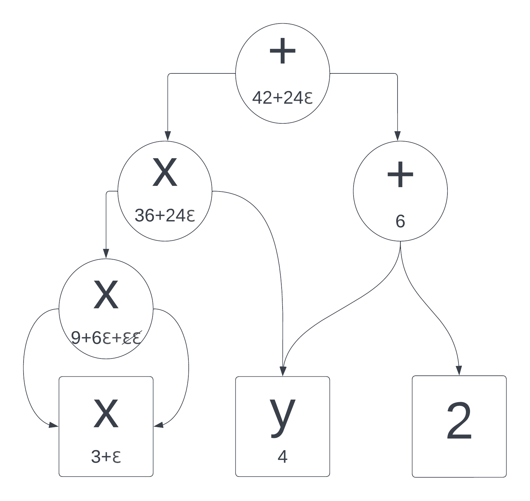
Figure 16: Forward-mode autodiff block diagram example

Rectified Linear Unit (ReLU)

In another example, a very well-known function called Rectified Linear Unit (ReLU), is one of the most used activation functions in machine learning models. We can write ReLU as $f(x)=\max(0,x)$ for what it’s derivative will be defined as:

$$f^{\prime}(x)=\begin{cases}1&x>0\\ 0&x<0\,.\end{cases}$$ (109)

This is the example where:

$$\lim_{h\to 0^{+}}\frac{f(x+h)-f(x)}{h}=1\neq\lim_{h\to 0^{-}}\frac{f(x+h)-f(x)}{h}=0\,.$$ (110)

Therefore, its derivative is not defined at $x=0$. The theory of why this case doesn’t pose any problem for reaching an optimal point when doing backpropagation is outside the scope of this text. However, we will see what the forward-mode automatic differentiation gives as a result. For it, we should first define, as usual, $f$ in the dual number space:

$$f\left((a,b)\right)=\begin{cases}(a,b)&a>0\\ (0,b)&a=0\\ (0,0)&a<0\,.\end{cases}$$ (111)

This definition is logical if we have chosen $\displaystyle\lim_{h^{+}\to 0}=\epsilon$ and must be changed if the left-sided limit is chosen. We therefore compute the value of $f(0,1)$ to see the value of the derivative at point $x=0$:

$$f(x+\epsilon) =\max(0,0.00...01)=0.00...01=(0,1)=(f(0),f^{\prime}(0))\,,$$ (112)

$$f\left((0,1)\right) =(0,1)\,.$$

We can see in Equation 112 that the forward-mode autodiff algorithm will yield the result of $Df(0)[\epsilon]=1$ which is an acceptable result for this case.

C.1.2 Complex forward-mode automatic differentiation

With the generalization to the complex case, $\epsilon$ now becomes complex, in the real case, we arbitrarily chose either the left or right-sided limit. Now, limitless directions are possible (phase), affecting, of course, the result of the derivative. Table 3 shows the derivative that is calculated when different values of $\epsilon$ are chosen.

Definition	One possibility for $\epsilon$
$\displaystyle\lim_{x\to 0}\frac{f(z+x)-f(z)}{x}$	$0.00...01$
$\displaystyle\lim_{y\to 0}\frac{f(z+i\,y)-f(z)}{y}$	$0.00...01\,i$
$\displaystyle\lim_{x\to 0,y\to 0}\frac{f(z+x-i\,y)-f(z)}{x+y}$	$0.00...01\,(1-i)$
$\displaystyle\lim_{x\to 0,y\to 0}\frac{f(z+x+i\,y)-f(z)}{x+y}$	$0.00...01\,(1+i)$

Table 3: Directional derivatives with respect to $\epsilon$.

The Table can be generalized to the following equation:

$$\nabla_{\epsilon}f=\lim_{h\to 0}\frac{f(z+h\,\epsilon)-f(z)}{h\,\epsilon}\,.$$ (113)

It is important to note that the module of $\epsilon$ is unimportant as long as it is small enough so that the analysis made in the last Section (Section C.1) stands.

For functions where the complex derivative exists, all possibilities will converge to the same value.

The first and second terms on Table 3 are used in the computation of Wirtinger Calculus, and it is not necessarily equal to the third term of the Table.

C.2 Reverse-mode automatic differentiation

Forward-mode automatic differentiation has many useful properties. First of all, as we have seen, the condition for the derivative to exist is not necessarily required for the method to yield a result that can be helpful when dealing with, in our case, non-holomorphic functions. Also, it allows finding a derivative value for any coded function, even containing loops or conditionals, as long as the primitives are defined. It is also natural for the algorithm to deal with the chain rule.

However, by taking a look at the example of Figure 16, if we now want to compute $\displaystyle\frac{\partial f}{\partial y}(3,4)$ we will need to compute $f(x,y+\epsilon)$, meaning that in order to know both $\displaystyle\frac{\partial f}{\partial x}(3,4)$ and $\displaystyle\frac{\partial f}{\partial y}(3,4)$ we will need to compute the algorithm twice. This can be exponentially costly for neural networks where there are sometimes even millions of trainable parameters from which we need to compute the partial derivative. Here is where reverse-mode automatic differentiation comes to the rescue enabling us to compute all partial derivatives at once.

C.2.1 Examples

In here we will show how reverse-mode autodiff can compute the previous both $\displaystyle\frac{\partial f}{\partial x}(3,4)$ and $\displaystyle\frac{\partial f}{\partial y}(3,4)$ of the previous example for forward-mode autodiff running the code once.

The first step is to compute $f(3,4)$, whose intermediate values are shown on the bottom right of each node. Each node was labeled as $n_{i}$ for clarity with $i\in[1,7]$. The output of $f(3,4)=n_{7}=42$ as expected.

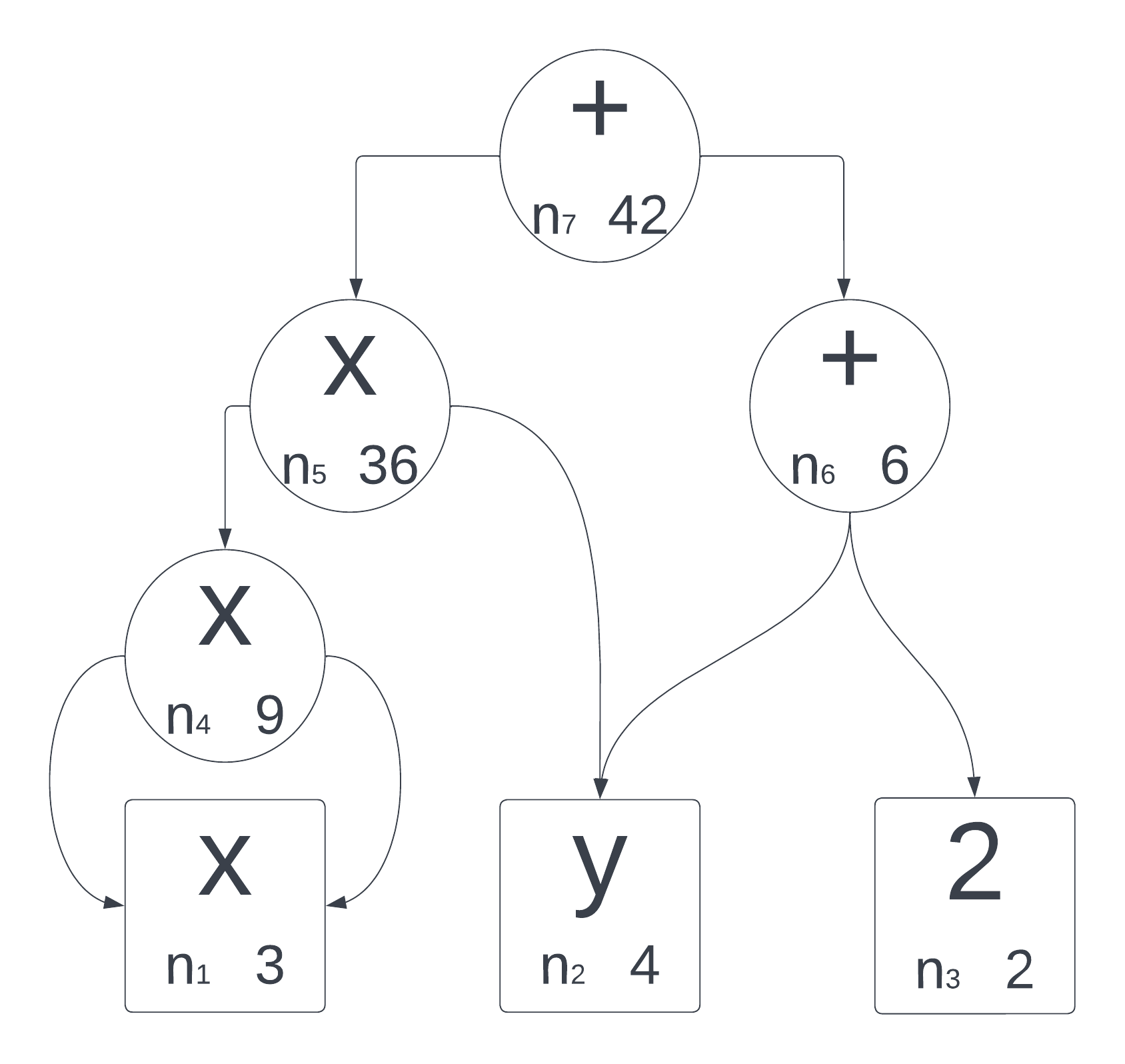
Figure 17: Reverse-mode autodiff block diagram example

Now all the partial derivatives $\displaystyle\frac{\partial f}{\partial n_{i}}$ are computed starting with $n_{7}$. Since $n_{7}$ is the output node, $\displaystyle\frac{\partial f}{\partial n_{7}}=1$. The chain rule is then used to compute the rest of the nodes by going down the graph. For example, to compute $\displaystyle\frac{\partial f}{\partial n_{5}}$ we use

$$\frac{\partial f}{\partial n_{5}}=\frac{\partial f}{\partial n_{7}}\frac{\partial n_{7}}{\partial n_{5}}\,,$$ (114)

and as we previously calculated $\displaystyle\frac{\partial f}{\partial n_{7}}$, we just need to compute the second term. This methodology will be repeated until all nodes’ partial derivatives are computed. Here is the full list of the partial derivatives:

• $\displaystyle\frac{\partial f}{\partial n_{7}}=1$,

• $\displaystyle\frac{\partial f}{\partial n_{6}}=\frac{\partial f}{\partial n_{7}}\frac{\partial n_{7}}{\partial n_{6}}=1$,

• $\displaystyle\frac{\partial f}{\partial n_{5}}=\frac{\partial f}{\partial n_{7}}\frac{\partial n_{7}}{\partial n_{5}}=1$,

• $\displaystyle\frac{\partial f}{\partial n_{4}}=\frac{\partial f}{\partial n_{5}}\frac{\partial n_{5}}{\partial n_{4}}=n_{2}=4$,

• $\displaystyle\frac{\partial f}{\partial y}=\frac{\partial f}{\partial n_{2}}=\frac{\partial f}{\partial n_{5}}\frac{\partial n_{5}}{\partial n_{2}}+\frac{\partial f}{\partial n_{6}}\frac{\partial n_{6}}{\partial n_{2}}=n_{4}+1=10$

• $\displaystyle\frac{\partial f}{\partial x}=\frac{\partial f}{\partial n_{1}}=\frac{\partial f}{\partial n_{5}}\frac{\partial n_{5}}{\partial n_{1}}+\frac{\partial f}{\partial n_{5}}\frac{\partial n_{5}}{\partial n_{1}}=n_{1}\cdot n_{4}+n_{1}\cdot n_{4}=3\cdot 4+3\cdot 4=24$.

This code has the advantage that all partial derivatives are computed at once which allows computing the values for a very high number of trainable parameters with less computational cost.

C.2.2 Complex reverse-mode automatic differentiation

In the following complex example, we will compute the reverse automatic differentiation on a complex multiplication operation $f=|(a+i\,b)(c+i\,d)|=a\,c-b\,d+a\,d+b\,c$, we know by definition that the derivative, using Wirtinger Calculus, is:

$$\frac{\partial f}{\partial(a+i\,b)} =\frac{\partial f}{\partial a}+i\,\frac{\partial f}{\partial b}=(c+d)+i\,(c-d)\,,$$ (115)

$$\frac{\partial f}{\partial(c+i\,d)} =\frac{\partial f}{\partial c}+i\,\frac{\partial f}{\partial d}=(a+b)+i\,(a-b)\,.$$ (116)

The following Figure 18 shows the block diagram of $f$.

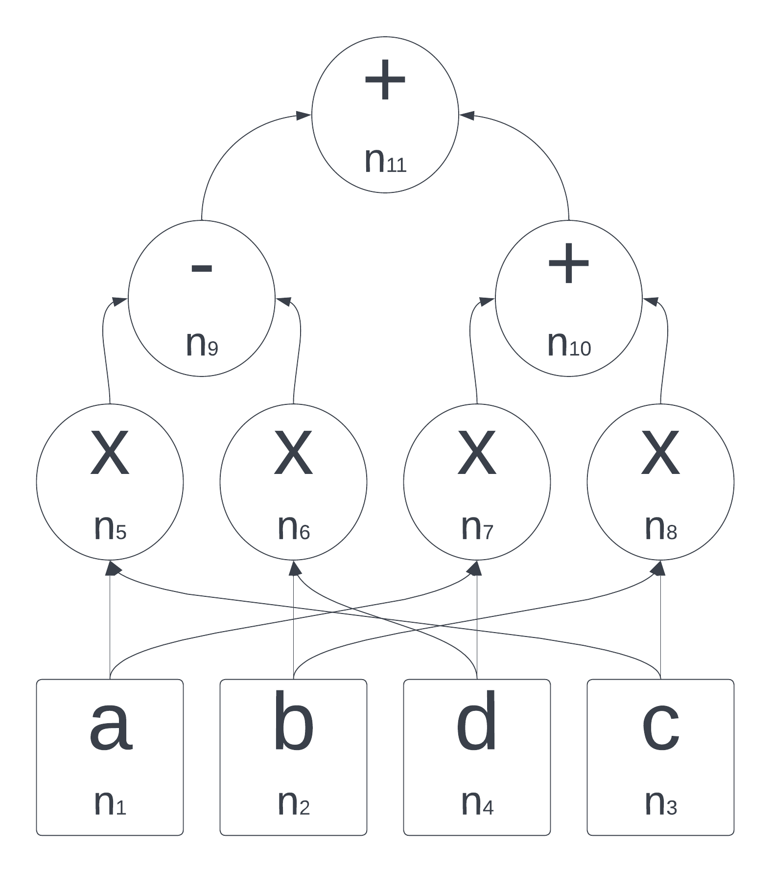
Figure 18: Complex reverse-mode autodiff block diagram example

Using the block diagram of Figure 18 we can compute the nodes as follows:

• $n_{1}=a$,

• $n_{2}=b$,

• $n_{3}=c$,

• $n_{4}=d$,

• $n_{5}=n_{1}\cdot n_{3}=a\cdot c$,

• $n_{6}=n_{2}\cdot n_{4}=b\cdot d$,

• $n_{7}=n_{1}\cdot n_{4}=a\cdot d$,

• $n_{8}=n_{2}\cdot n_{3}=b\cdot c$,

• $n_{9}=n_{5}-n_{6}=a\,c-b\,d$,

• $n_{10}=n_{7}+n_{8}=a\,d+b\,c$,

• $f=n_{11}=n_{10}+n_{9}=a\,c-b\,d+a\,d+b\,c$.

We now perform the reverse-mode backpropagation starting from the last node ($n_{11}$) and go back using the previously computed values to extract the partial derivative of $f=n_{11}$ with respect to every node.

• $\displaystyle\frac{\partial f}{\partial n_{11}}=\frac{\partial n_{11}}{\partial n_{11}}=1$,

• $\displaystyle\frac{\partial n_{11}}{\partial n_{10}}=1$,

• $\displaystyle\frac{\partial n_{11}}{\partial n_{9}}=1$,

• $\displaystyle\frac{\partial n_{11}}{\partial n_{8}}=\frac{\partial n_{11}}{\partial n_{10}}\frac{\partial n_{10}}{\partial n_{8}}=1$,

• $\displaystyle\frac{\partial n_{11}}{\partial n_{7}}=\frac{\partial n_{11}}{\partial n_{10}}\frac{\partial n_{10}}{\partial n_{7}}=1$,

• $\displaystyle\frac{\partial n_{11}}{\partial n_{6}}=\frac{\partial n_{11}}{\partial n_{9}}\frac{\partial n_{9}}{\partial n_{6}}=-1$,

• $\displaystyle\frac{\partial n_{11}}{\partial n_{5}}=\frac{\partial n_{11}}{\partial n_{9}}\frac{\partial n_{9}}{\partial n_{5}}=1$,

• $\displaystyle\frac{\partial f}{\partial d}=\frac{\partial n_{11}}{\partial n_{4}}=\frac{\partial n_{11}}{\partial n_{7}}\frac{\partial n_{7}}{\partial n_{4}}+\frac{\partial n_{11}}{\partial n_{6}}\frac{\partial n_{6}}{\partial n_{4}}=n_{1}-n_{2}=a-b$,

• $\displaystyle\frac{\partial f}{\partial c}=\frac{\partial n_{11}}{\partial n_{3}}=\frac{\partial n_{11}}{\partial n_{8}}\frac{\partial n_{8}}{\partial n_{3}}+\frac{\partial n_{11}}{\partial n_{5}}\frac{\partial n_{5}}{\partial n_{3}}=n_{2}+n_{1}=b+a$,

• $\displaystyle\frac{\partial f}{\partial b}=\frac{\partial n_{11}}{\partial n_{2}}=\frac{\partial n_{11}}{\partial n_{6}}\frac{\partial n_{6}}{\partial n_{2}}+\frac{\partial n_{11}}{\partial n_{8}}\frac{\partial n_{8}}{\partial n_{2}}=n_{3}-n_{4}=c-d$,

• $\displaystyle\frac{\partial f}{\partial a}=\frac{\partial n_{11}}{\partial n_{1}}=\frac{\partial n_{11}}{\partial n_{5}}\frac{\partial n_{5}}{\partial n_{1}}+\frac{\partial n_{7}}{\partial n_{1}}\frac{\partial n_{7}}{\partial n_{1}}=n_{3}+n_{4}=c+d$.

Now, if we consider $\partial f/\partial(a+i\,b)=\partial f/\partial a+i\,\partial f/\partial b$ and replace the values we obtained in the previous list, we get the same result as in Equation 115.

References

- [1] A. Hirose and S. Yoshida. Generalization characteristics of complex-valued feedforward neural networks in relation to signal coherence. IEEE Transactions on Neural Networks and learning systems, 23(4):541–551, 2012.
- [2] R. Hänsch and O. Hellwich. Classification of polarimetric SAR data by complex-valued neural networks. In Proc. ISPRS Hannover Workshop, High-Resolution Earth Imag. Geospatial Inf., volume 37, 2009.
- [3] A. Hirose. Complex-valued Neural Networks, volume 400. Springer Science & Business Media, 2012.
- [4] A. Hirose. Complex-valued neural networks: The merits and their origins. In 2009 International Joint Conference on Neural Networks, pages 1237–1244. IEEE, 2009.
- [5] N. Mönning and S. Manandhar. Evaluation of Complex-Valued Neural Networks on Real-Valued Classification Tasks. arXiv preprint arXiv:1811.12351, 2018.
- [6] Philipp H. W. Hoffmann. A Hitchhiker’s guide to automatic differentiation. Numerical Algorithms, 72(3):775–811, 2016.
- [7] Chiheb Trabelsi, Olexa Bilaniuk, Ying Zhang, Dmitriy Serdyuk, Sandeep Subramanian, Joao Felipe Santos, Soroush Mehri, Negar Rostamzadeh, Yoshua Bengio, and Christopher J Pal. Deep complex networks. arXiv preprint arXiv:1705.09792, 2017.
- [8] Jesper Sören et al. Dramsch. Complex-Valued Neural Networks in Keras with Tensorflow, 2019.
- [9] Maxime W. Matthès, Yaron Bromberg, Julien de Rosny, and Sébastien M. Popoff. Learning and avoiding disorder in multimode fibers. Phys. Rev. X, 11:021060, Jun 2021.
- [10] J Agustin Barrachina. NEGU93/cvnn. https://doi.org/10.5281/zenodo.4452131, January 2021.
- [11] J. A. Barrachina. Complex-Valued Neural Networks (CVNN). https://github.com/NEGU93/cvnn, 2019.
- [12] A. Hirose. Complex-valued Neural Networks: Advances and applications, volume 18. John Wiley & Sons, 2013.
- [13] W. Wirtinger. Zur formalen Theorie der Funktionen von mehr komplexen Veränderlichen. Mathematische Annalen, 97(1):357–375, Dec 1927.
- [14] Ken Kreutz-Delgado. The Complex Gradient Operator and the CR-Calculus. arXiv e-prints, page arXiv:0906.4835, Jun 2009.
- [15] Robert F. H. Fischer. Appendix A: Wirtinger Calculus, pages 405–413. John Wiley & Sons, Ltd, 2005.
- [16] A. Hirose, F. Amin, and K. Murase. Learning Algorithms in Complex-Valued Neural Networks using Wirtinger Calculus. In Complex-Valued Neural Networks: Advances and Applications, pages 75–102. IEEE, 2013.
- [17] M. F. Amin, M. I. Amin, A. Y. H. Al-Nuaimi, and K. Murase. Wirtinger Calculus Based Gradient Descent and Levenberg-Marquardt Learning Algorithms in Complex-Valued Neural Networks. In Neural Information Processing, pages 550–559, Berlin, Heidelberg, 2011. Springer Berlin Heidelberg.
- [18] Hualiang Li and Tülay Adalı. Complex-valued adaptive signal processing using nonlinear functions. EURASIP Journal on Advances in Signal Processing, 2008(1):765615, 2008.
- [19] C. Boeddeker, P. Hanebrink, L. Drude, J. Heymann, and Reinhold Haeb-Umbach. On the computation of complex-valued gradients with application to statistically optimum beamforming. arXiv preprint arXiv:1701.00392, 2017.
- [20] Raphael Hunger. An introduction to complex differentials and complex differentiability. Technical report, Munich University of Technology, Inst. for Circuit Theory and Signal Processing, 2007.
- [21] Aurélien Géron. Hands-On Machine Learning with Scikit-Learn, Keras, and TensorFlow: Concepts, Tools, and Techniques to Build Intelligent Systems. O’Reilly Media, 2019.
- [22] Ronny Hänsch and Olaf Hellwich. Classification of polarimetric SAR data by complex-valued Neural Networks. In ISPRS Workshop High-Resolution Earth Imaging for Geospatial Information, volume 38, pages 4–7, 2009.
- [23] Z. Zhang, H. Wang, F. Xu, and Y.-Q. Jin. Complex-valued convolutional neural network and its application in polarimetric SAR image classification. IEEE Transactions on Geoscience and Remote Sensing, 55(12):7177–7188, 2017.
- [24] bkkm16. What we should use align corners to False?, 2019.
- [25] Matthew D Zeiler, Dilip Krishnan, Graham W Taylor, and Rob Fergus. Deconvolutional networks. In 2010 IEEE Computer Society Conference on Computer Vision and Pattern Recognition, pages 2528–2535. IEEE, 2010.
- [26] I. Zafar, G. Tzanidou, R. Burton, N. Patel, and L. Araujo. Hands-on convolutional neural networks with TensorFlow: Solve computer vision problems with modeling in TensorFlow and Python. Packt Publishing Ltd, Birmingham, UK, 2018.
- [27] J. A. Barrachina, C. Ren, G. Vieillard, C. Morisseau, and J.-P. Ovarlez. About the Equivalence Between Complex-Valued and Real-Valued Fully Connected Neural Networks - Application to PolInSAR Images. In 2021 IEEE 31st International Workshop on Machine Learning for Signal Processing (MLSP), pages 1–6, 2021.
- [28] Simone Scardapane, Steven Van Vaerenbergh, Amir Hussain, and Aurelio Uncini. Complex-valued Neural Networks with nonparametric activation functions. IEEE Transactions on Emerging Topics in Computational Intelligence, 4(2):140–150, 2018.
- [29] J. Bassey, L. Qian, and X. Li. A survey of complex-valued Neural Networks. arXiv preprint arXiv:2101.12249, 2021.
- [30] ChiYan Lee, Hideyuki Hasegawa, and Shangce Gao. Complex-Valued Neural Networks: A Comprehensive Survey. IEEE/CAA Journal of Automatica Sinica, 9(8):1406–1426, 2022.
- [31] Y. Kuroe, M. Yoshid, and T. Mori. On activation functions for complex-valued Neural Networks: existence of energy functions. In Artificial Neural Networks and Neural Information Processing, ICANN/ICONIP 2003, pages 985–992. Springer, 2003.
- [32] Taehwan Kim and Tülay Adali. Approximation by fully complex MLP using elementary transcendental activation functions. In Neural Networks for Signal Processing XI: Proceedings of the 2001 IEEE Signal Processing Society Workshop (IEEE Cat. No.01TH8584), pages 203–212. IEEE, 2001.
- [33] Taehwan Kim and Tülay Adali. Complex backpropagation Neural Network using elementary transcendental activation functions. In 2001 IEEE International Conference on Acoustics, Speech, and Signal Processing. Proceedings (Cat. No. 01CH37221), volume 2, pages 1281–1284. IEEE, 2001.
- [34] Naum N. Ajzenberg and Zivko Tošić. A generalization of the threshold functions. Publikacije Elektrotehničkog Fakulteta. Serija Matematika i Fizika, pages 97–99, 1972.
- [35] N. N. Aizenberg, Yu. L. Ivas’kiv, D. A. Pospelov, and G. F. Khudyakov. Multivalued threshold functions. Cybernetics, 9(1):61–77, 1973.
- [36] G. M. Georgiou and C. Koutsougeras. Complex domain backpropagation. IEEE Transactions on Circuits and Systems II: Analog and Digital Signal Processing, 39(5):330–334, 1992.
- [37] A. Krizhevsky, I. Sutskever, and G. Hinton. Imagenet classification with deep convolutional neural networks. In Advances in neural information processing systems, pages 1097–1105, 2012.
- [38] Y. Cao, Y. Wu, P. Zhang, W. Liang, and M. Li. Pixel-wise PolSAR image classification via a novel complex-valued deep fully convolutional network. Remote Sensing, 11(22):2653, 2019.
- [39] Nitzan Guberman. On Complex Valued Convolutional Neural Networks. CoRR, abs/1602.09046, 2016.
- [40] Martin Arjovsky, Amar Shah, and Yoshua Bengio. Unitary evolution recurrent Neural Networks. In International Conference on Machine Learning, pages 1120–1128. PMLR, 2016.
- [41] Patrick Virtue, X Yu Stella, and Michael Lustig. Better than real: Complex-valued neural nets for MRI fingerprinting. In 2017 IEEE international conference on image processing (ICIP), pages 3953–3957. IEEE, 2017.
- [42] Ian Goodfellow, Yoshua Bengio, and Aaron Courville. Deep Learning. MIT Press, 2016. http://www.deeplearningbook.org.
- [43] R. Hänsch. Complex-Valued Multi-Layer Perceptrons - An Application to Polarimetric SAR Data. Photogrammetric Engineering & Remote Sensing, 76(9):1081–1088, 2010.
- [44] X. Glorot and Y. Bengio. Understanding the difficulty of training deep feedforward neural networks. In Proceedings of the thirteenth international conference on artificial intelligence and statistics, pages 249–256, 2010.
- [45] Lord Rayleigh. XII. On the resultant of a large number of vibrations of the same pitch and of arbitrary phase. The London, Edinburgh, and Dublin Philosophical Magazine and Journal of Science, 10(60):73–78, 1880.
- [46] Gilles Vieillard. Reconnaissance de signaux radar par apprentissage profond. Technical Report RA 2/26398 DEMR, ONERA - Département Électromagnétisme et Radar (DEMR), feb 2018.
- [47] SL Hahn. Hilbert Transforms in Signal Processing. Artech House, Norwood, USA, 1996.
- [48] Godfrey H Hardy. The Theory of Cauchy’s Principal Values. (Third Paper: Differentiation and Integration of Principal Values.). Proceedings of the London Mathematical Society, 1(1):81–107, 1902.
- [49] Godfrey H Hardy. The Theory of Cauchy’s Principal Values.(Fourth Paper: The Integration of Principal Values—Continued—with Applications to the Inversion of Definite Integrals). Proceedings of the London Mathematical Society, 2(1):181–208, 1909.
- [50] F King. Hilbert Transforms: Encyclopedia of Mathematics and its Applications 124, 2009.
- [51] David Hilbert. Fundamentals of a general theory of linear integral equations, volume 3. BG Teubner, 1912.
- [52] Godfrey H Hardy. Notes on some points in the integral calculus (LVIII). On Hilbert transforms. Messenger of Math., 54:20–27, 1924.
- [53] Godfrey H. Hardy. Notes on some points in the integral calculus (LIX). On Hilbert transforms. Messenger of Math., 54:81–88, 1924.
- [54] R. de L. Kronig. On the theory of dispersion of x-rays. Journal of the Optical Society of America, 12(6):547–557, 1926.
- [55] Hendrik Anthony Kramers. La diffusion de la lumière par les atomes. In Atti Cong. Intern. Fisica (Transactions of Volta Centenary Congress) Como, volume 2, pages 545–557, 1927.
- [56] John R Carson. Electric circuit theory and the operational calculus. The Bell System Technical Journal, 5(2):336–384, 1926.
- [57] Dennis Gabor. Theory of communications. J. Inst. Elec. Eng, 93:429–457, 1946.
- [58] Kaiming He, Xiangyu Zhang, Shaoqing Ren, and Jian Sun. Delving deep into rectifiers: Surpassing human-level performance on Imagenet classification. In Proceedings of the IEEE International Conference on Computer Vision, pages 1026–1034, 2015.
- [59] Simon S Haykin. Adaptive filter theory. Pearson Education India, 2005.
- [60] N. Benvenuto and F. Piazza. On the complex backpropagation algorithm. IEEE Transactions on Signal Processing, 40(4):967–969, April 1992.
- [61] Louis B. Rall. The arithmetic of differentiation. Mathematics Magazine, 59(5):275–282, 1986.
- [62] B. D. Hall. Calculating measurement uncertainty for complex-valued quantities. Measurement Science and Technology, 14(3):368, 2003.
- [63] Barak A Pearlmutter and Jeffrey Mark Siskind. Lazy multivariate higher-order forward-mode ad. ACM SIGPLAN Notices, 42(1):155–160, 2007.
- [64] Louis B. Rall. Differentiation and generation of taylor coefficients in Pascal-SC. In A New Approach to Scientific Computation, pages 291–309. Elsevier, 1983.
- [65] Gershon Kedem. Automatic differentiation of computer programs. ACM Transactions on Mathematical Software (TOMS), 6(2):150–165, 1980.