A Superdirective Beamforming Approach with Impedance Coupling and Field Coupling for Compact Antenna Arrays

Abstract

In most multiple-input multiple-output (MIMO) communication systems, the antenna spacing is generally no less than half a wavelength. It helps to reduce the mutual coupling and therefore facilitate the system design. The maximum array gain equals the number of antennas in this settings. However, when the antenna spacing is made very small, the array gain of a compact array can be proportional to the square of the number of antennas - a value much larger than the traditional array. To achieve this so-called “superdirectivity” however, the calculation of the excitation coefficients (beamforming vector) is known to be a challenging problem. In this paper, we address this problem with a novel double coupling-based superdirective beamforming method. In particular, we categorize the antenna coupling effects to impedance coupling and field coupling. By characterizing these two coupling in model, we derive the beamforming vector for superdirective arrays. In order to obtain the field coupling matrix, we propose a spherical wave expansion approach, which is effective in both simulations and realistic scenarios. Moreover, a prototype of the independently controlled superdirective antenna array is developed. Full-wave electromagnetic simulations and real-world experiments validate the effectiveness of our proposed approaches, and superdirectivity is achieved in reality by a compact array with 4 and 5 dipole antennas.

I Introduction

As one of the key technologies of the fifth generation (5G) mobile communication systems, massive MIMO is being commercialized world wide with the deployments of 5G networks [2]. The authors of [3] predicted the large gain of the spectral efficiency when the number of antennas at the base station tends to infinity. In practice however, the antenna spacing is generally no less than half a wavelength. One of the major reasons is to make the coupling effect between antennas negligible and therefore facilitate the system design. However, it also leads to the limitation of the number of antennas for an antenna panel with a fixed aperture. In recent years, with the further demand for spectral efficiency, the possibility of deploying super dense antenna arrays at the base station has been considered by researchers[4][5] [6]. The mutual coupling between antennas in such scenarios has to be considered. In fact, the coupling effect is not all negative. In a compact array containing $M$ antennas with much smaller antenna spacing than half a wavelength, the strong coupling is the foundation of the superdirectivity, where the beamforming gain may reach $M^{2}$, instead of $M$ as in traditional MIMO theory.

In general, the electromagnetic waves radiated by antennas can be categorized into propagating waves and evanescent waves [7], and the coupling between antennas is caused by the joint action of these two kinds of waves. When the antenna spacing is much smaller than half a wavelength, the effect of the evanescent wave is more obvious than the propagating wave, making the coupling between antennas extremely strong [8][9]. The role of coupling in an antenna array, however, is often ignored in traditional communication researches[10]. In theory, if the amplitude and phase of each antenna excitation are controlled precisely, this strong coupling can cause the antenna array to have the superdirectivity[4][11]. According to traditional communication theory, the array gain is proportional to the number of antennas $M$. However in [12], Uzkov proved that the directivity of an isotropic linear array of $M$ antennas can reach $M^{2}$ when the spacing between antennas approaches zero. If the base station is equipped with a large number of antennas, the array gain improvement is more significant[13].

Despite the remarkable potential of gain improvement introduced by superdirective antenna arrays, there are several challenges that hinder its practical realization. In particular, it appeared that the precision of superdirective beamforming vector can affect the performance of the antenna array[9]. And the calculation of the beamforming vector is known as a very challenging problem. This is related to the strong antenna mutual coupling which is hard to characterize in superdirective arrays. The work of [9] initiates the practical measurements of a two-element superdirective array, whose beamforming vector calculation ignores the mutual field coupling between antennas. The authors of [14] proposes a decoupling array structure to enhance the directivity, which may lead to high hardware complexity, especially when the number of antennas is large. A compact parasitic four-element superdirective array is designed in [15], yet the method depends on the accuracy of simulation tools and may introduce unwanted negative resistance to array design.

In this paper, we revisit the problem of superdirective beamforming vector calculation by taking a double-coupling effect of antenna arrays into consideration. We find there are two sorts of coupling which we call impedance coupling and field coupling respectively in compact antenna arrays. The impedance coupling represents the power radiation interaction between antennas, or regarded as the mutual impedance matrix of the array in free space. While the filed coupling leads to the distortion of the radiation pattern of every antenna in the array. We propose a novel coupling matrix-based method to depict the field coupling of superdirective antenna arrays. The spherical wave expansion method is utilized to calculate the field coupling matrix. More specifically, our method is based on the fact that the coupling field can be viewed as the antenna array excited with a specific beamforming vector. By leveraging the electric field containing the coupling information, the field coupling matrix of antenna arrays is derived precisely in simulations. Moreover, in practice the electromagnetic environment is more complex than the ideal simulation conditions. It is meaningful to model the coupling of antenna arrays with realistic measured data. To this end, we further devise a measurement scheme to compute the coupling matrices of a practical antenna array.

The contributions of this paper are as follows:

• We propose to introduce a field coupling matrix to the superdirective antenna array model. In the traditional superdirective beamforming method, the field coupling is not considered, which impairs the directivity. For an antenna array with small spacing, the field coupling plays a key role in characterizing the interactions between the antennas. Substantial directivity improvements over existing beamforming methods are observed in simulations and measurements.

• We propose a spherical wave expansion-based field coupling matrix calculation approach, which extracts the coupling information in the active element pattern. We prove that the field coupling matrix has the unique solution for an antenna array, and itself has the ability to fully characterize the distorted coupling field. Simulation results also show that the field coupling matrix computed by our method is precise.

• We further propose a practical method to calculate the coupling matrix based on the realistic measurement data. In practice, there are some conditions that are difficult to be considered by simulations, e.g., the non-ideal manufacturing technology of the antennas, the radiation effect of the coaxial line, the influence of the connectors, etc., which make the actual radiation environment of the antenna array quite different from the ideal simulation. The proposed method is able to cope with these practical limitations.

• We build a prototype of the superdirective antenna array. To the best of our knowledge, the realization of independently controlled four or five-channel superdirective antenna arrays has not been presented so far. A beamforming control board, which offers 7-bit amplitude precision and 8-bit phase precision, is designed to excite the antenna array. The superdirective antenna arrays with four and five elements are tested in a microwave anechonic chamber. Our proposed methods are validated with this platform in the microwave anechonic chamber, and the gain of directivity over existing methods is confirmed with real-world measurements.

This paper is organized as follows: In Sec. II we introduce the superdirective beamforming method based on array theory. In Sec. III we propose the coupling matrix and spherical wave expansion-based superdirective beamforming approach. In Sec. IV the numerical results including simulations and practical measurements are shown. Finally, conclusions are drawn in Sec. V.

Notations: The boldface font stands for vector and matrix. ${{\bf{X}}^{\dagger}},{{\bf{X}}^{T}},{{\bf{X}}^{*}},$ and ${{\bf{X}}^{H}}$ denote the Moore–Penrose pseudoinverse, transpose, conjugation, and Hermitian transpose of $\bf{X}$, respectively. ${\mathbb{C}^{a\times b}}$ is a matrix space with $a$ rows and $b$ columns. $\left|{\bf{x}}\right|$ denotes the absolute value of $\bf{x}$ and ${\left\|{\bf{X}}\right\|_{2}}$ is the second-order induced norm of $\bf{X}$. $\buildrel\Delta\over{=}$ refers to the definition symbol.

II Beamforming of superdirective arrays based on array theory

According to [12], only when at least two requirements are met can an antenna array achieve superdirectivity. The first is that the spacing between two neighboring antennas should be less than half a wavelength, which is simple to accomplish. Second, the amplitude and phase of the excitation coefficient of each antenna should be properly calculated and controlled. However, due to the strong coupling effect between antennas, the second condition is not easy to satisfy. This section will present the traditional method to calculate the superdiretive beamforming vector based on array theory.

Consider a uniform linear array with $M$ antennas, each of which has the same pattern function of $g(\theta,\phi)$, where $\theta$ and $\phi$ stand for the far-field location in a spherical coordinate system. Without loss of generality, the first antenna is at the center of the Cartesian coordinate system and the other antennas are distributed evenly along the positive half of the $y$-axis, with a spacing of $d$. Consequently, the complex far-field pattern of this antenna array is given by

$$f(\theta,\phi)=\sum_{m=1}^{M}a_{m}g(\theta,\phi)e^{jk\mathbf{\hat{r}}\cdot\mathbf{r}_{m}},$$ (1)

where $a_{m}$ is the complex excitation coefficient consistent with the current on the $m$-th antenna, $k=2\pi/\lambda$ is the wave number, $\mathbf{\hat{r}}$ is the unit vector of the far-field direction $(\theta,\phi)$ in the spherical coordinate system, and $\mathbf{r}_{m}$ is the position of the $m$-th antenna. As a result, the directivity factor at $(\theta_{0},\phi_{0})$ can be calculated as

$$D(\theta_{0},\phi_{0})=$$

$$\quad\dfrac{|\sum_{m=1}^{M}a_{m}g(\theta_{0},\phi_{0})e^{jk\mathbf{\hat{r}}_{0}\cdot\mathbf{r}_{m}}|^{2}}{\frac{1}{4\pi}\int_{0}^{2\pi}\int_{0}^{\pi}|\sum_{m=1}^{M}a_{m}g(\theta,\phi)e^{jk\mathbf{\hat{r}}\cdot\mathbf{r}_{m}}|^{2}\sin\theta d\theta d\phi},$$ (2)

where $\mathbf{\hat{r}}_{0}$ is the unit vector in the direction $(\theta_{0},\phi_{0})$.

For deriving the maximum directivity of an antenna array, the expression of (II) is not straightforward and is thus worthy of further simplification. The denominator of (II) can be expanded as

$$\frac{1}{4\pi}\int_{0}^{2\pi}\int_{0}^{\pi}\left|\sum_{m=1}^{M}a_{m}g(\theta,\phi)e^{jk\mathbf{\hat{r}}\cdot\mathbf{r}_{m}}\right|^{2}\sin\theta d\theta d\phi$$

$$=\frac{1}{4\pi}\int_{0}^{2\pi}\int_{0}^{\pi}\sum_{n=1}^{M}\sum_{m=1}^{M}a_{n}a_{m}^{*}|g(\theta,\phi)|^{2}e^{jk\mathbf{\hat{r}}\cdot\mathbf{r}_{n}}e^{-jk\mathbf{\hat{r}}\cdot\mathbf{r}_{m}}\sin\theta d\theta d\phi$$

$$=\sum_{n=1}^{M}\sum_{m=1}^{M}a_{n}a_{m}^{*}\frac{1}{4\pi}\int_{0}^{2\pi}\int_{0}^{\pi}|g(\theta,\phi)|^{2}e^{jk\mathbf{\hat{r}}\cdot\mathbf{r}_{n}}e^{-jk\mathbf{\hat{r}}\cdot\mathbf{r}_{m}}\sin\theta d\theta d\phi,$$ (3)

where the $a_{n}^{*}$ represents the conjugate of the complex value $a_{n}$.

For the integral items in (II), we introduce the following equation:

$$z_{mn}\buildrel\Delta\over{=}\frac{1}{4\pi}\int_{0}^{2\pi}\int_{0}^{\pi}|g(\theta,\phi)|^{2}e^{jk\mathbf{\hat{r}}\cdot\mathbf{r}_{m}}e^{-jk\mathbf{\hat{r}}\cdot\mathbf{r}_{n}}\sin\theta d\theta d\phi.$$ (4)

As the power radiated by the antenna array is active power, $z_{mn}$ represents the real part of the normalized mutual impedance between the $m$-th antenna and the $n$-th antenna[16]. Then (II) can be rewritten as

$$\sum_{m=1}^{M}\sum_{n=1}^{M}a_{m}a^{*}_{n}\frac{1}{4\pi}\int_{0}^{2\pi}\int_{0}^{\pi}|g(\theta,\phi)|^{2}e^{jk\mathbf{\hat{r}}\cdot\mathbf{r}_{m}}e^{-jk\mathbf{\hat{r}}\cdot\mathbf{r}_{n}}\sin\theta d\theta d\phi$$

$$=\sum_{m=1}^{M}\sum_{n=1}^{M}a_{m}a^{*}_{n}z_{mn}.$$ (5)

For the simplicity of notations, (II) is further rewritten using two vectors $\mathbf{a},\mathbf{e}\in\mathbb{C}^{M\times 1}$

$$D=\dfrac{\mathbf{a}^{T}\mathbf{e}\mathbf{e}^{H}\mathbf{a}^{*}}{\mathbf{a}^{T}\mathbf{Z}\mathbf{a}^{*}},$$ (6)

where $\mathbf{a}$ denotes the beamforming vector

$$\mathbf{a}=\left[a_{1},\,a_{2},\,\cdots,\,a_{M}\right]^{T},$$ (7)

and

$$\mathbf{e}=\left[e^{jk\mathbf{\hat{r}}\cdot\mathbf{r}_{1}}k(\theta,\phi),\,e^{jk\mathbf{\hat{r}}\cdot\mathbf{r}_{2}}k(\theta,\phi),\,\cdots,\,e^{jk\mathbf{\hat{r}}\cdot\mathbf{r}_{M}}k(\theta,\phi)\right]^{T}.$$ (8)

$\mathbf{Z}\in\mathbb{C}^{M\times M}$ stands for the real part of the normalized impedance matrix, which can be considered as the impedance coupling between antennas

$$\mathbf{Z}=\left[\begin{array}[]{ccc}z_{11}&\ldots&z_{1M}\\ \vdots&\ddots&\vdots\\ z_{M1}&\cdots&z_{MM}\end{array}\right].$$ (12)

Note that (6) is in the form of Rayleigh quotient, the directivity maximization problem can be handled by finding the derivative of (6) with respect to the vector $\mathbf{a}$ as follow:

$$\frac{\partial D}{\partial\mathbf{a}}=\frac{2\mathbf{e}\mathbf{e}^{H}\mathbf{a}^{*}}{\mathbf{a}^{T}\mathbf{Z}\mathbf{a}^{*}}-2D\frac{\mathbf{Z}\mathbf{a}^{*}}{\mathbf{a}^{T}\mathbf{Z}\mathbf{a}^{*}}.$$ (13)

Letting the above formula equal to zero yields

$$\mathbf{e}\mathbf{e}^{H}\mathbf{a}^{*}=D\mathbf{Z}\mathbf{a}^{*}.$$ (14)

It can be found that (14) is a generalized eigenvalue problem of the form $\mathbf{A}\mathbf{x}=\lambda\mathbf{B}\mathbf{x}$, where $\mathbf{A}$ and $\mathbf{B}$ are matrices, and $\mathbf{x}$ is the generalized eigenvector of $\mathbf{A}$ and $\mathbf{B}$, while $\lambda$ is the corresponding generalized eigenvalue. Multiplying both sides of (14) by $\mathbf{Z}^{-1}$ yields

$$\mathbf{Z}^{-1}\mathbf{e}\mathbf{e}^{H}\mathbf{a}^{*}=D\mathbf{a}^{*}.$$ (15)

The eigenvalue of the above equation has only one solution as demonstrated in [16]. Consequently, the only one non-zero eigenvalue of $\mathbf{Z}^{-1}\mathbf{e}\mathbf{e}^{H}$ is the maximum value of the directivity factor $D_{\max}$. Hence, (15) can be rewritten as

$$\mathbf{Z}^{-1}\mathbf{e}\mathbf{e}^{H}\mathbf{a}^{*}=D_{\max}\mathbf{a}^{*}.$$ (16)

Since

$$\mathbf{Z}^{-1}\mathbf{e}\mathbf{e}^{H}\mathbf{a}^{*} =\mathbf{Z}^{-1}\mathbf{e}(\mathbf{e}^{H}\mathbf{a}^{*})$$

$$=\xi\mathbf{Z}^{-1}\mathbf{e},$$ (17)

where $\xi=\mathbf{e}^{H}\mathbf{a}^{*}$ is a scalar, the beamforming vector making the antenna array produce the maximum directivity factor can thus be written as

$$\mathbf{a}=\frac{\xi}{D_{\max}}\mathbf{Z}^{-1}\mathbf{e}^{*}=\mu\mathbf{Z}^{-1}\mathbf{e}^{*},$$ (18)

where the scalar $\mu$ is defined as $\mu={\xi}/{D_{\max}}$. Substituting (18) into (6), we obtain the maximum directivity factor as

$$D_{\max}=\mathbf{e}^{H}\mathbf{Z}^{-1}\mathbf{e}.$$ (19)

However, the above derivation process ignores the field coupling between the antennas. In practice, strong field coupling effect will occur between antennas when the spacing is small, making the radiation pattern emitted by one antenna distorted by the influence of surrounding antennas. Whereas in (1), if $a_{n}$ is set to 1 and $a_{m},m=2,\cdots,M,m\neq n$, are set to 0, the $f(\theta,\phi)$ would be $a_{n}k(\theta,\phi)e^{jk\mathbf{\hat{r}}\cdot\mathbf{r}_{n}}$ which indicates that the radiation pattern of the $n$-th antenna is not influenced by any other antennas, which is unrealistic. Due to the small spacing required by the superdirective antenna array, mutual field coupling should not be overlooked. As a result, the beamforming vector based on the traditional approach (18) may not be applicable to make an antenna array produce maximum directivity. Next, to achieve a more realistic superdirectivity, we will propose a superdirective array analysis approach based on the impedance coupling and field coupling matrices.

III Proposed superdirective beamforming based on double couplings

In this section, we propose the superdirective beamforming approach which considers both the impedance coupling effect and the field coupling effect. We first show how to obtain the superdirective beamforming vector with the full-wave simulations, which is the foundation of our superdirective beamforming realization method in practice. Then, since there are still some factors not considered in the simulations, we further propose a measurement-based approach to acquire the impedance coupling and field coupling matrices, which will help produce superdirectivity in practice.

III-A Full-wave simulation-based acquisition of the superdirective beamforming vector

Since the superdirectivity is produced only when the antenna spacing is small, the field coupling effect should not be ignored when deriving the beamforming vector. In this section, we propose to characterize the field coupling effect between antennas with a coupling matrix, which is obtained using spherical wave expansion method and full-wave simulation tools.

The spherical wave expansion method is often used in antenna measurements to calculate the radiated far field from the measured spherical near field [17]. It can also decompose the electromagnetic field into a series of spherical wave coefficients using a set of orthogonal spherical wave basis. In this method, the electric field $\mathbf{E}(\theta,\phi)$ radiated by the antenna in the far-field region is expanded as

$$\mathbf{E}(\theta,\phi) =k\sqrt{\eta}\sum_{s=1}^{2}{\sum_{n=1}^{N}{\sum_{m=-n}^{n}{Q_{s,m,n}}}}\mathbf{K}_{s,m,n}(\theta,\phi)$$

$$=k\sqrt{\eta}\sum_{s,m,n}{Q_{s,m,n}}\mathbf{K}_{s,m,n}(\theta,\phi),$$ (20)

where

$$\mathbf{E}(\theta,\phi)=[E_{\hat{\theta}}(\theta,\phi),E_{\hat{\phi}}(\theta,\phi)],$$ (21)

with the subscripts $\hat{\theta}$ and $\hat{\phi}$ denoting the $\theta$-component and $\phi$-component respectively. $\eta$ is the medium intrinsic impedance. $N$ is a truncated constant, and the larger $N$ is, the better the above equation (III-A) fits the real electric field. In practice, one may take $N=kr_{0}+10$, where $r_{0}$ is the minimum radius of the spherical surface that can enclose the antenna. $Q_{s,m,n}$ is the spherical wave coefficient. $s=1,2$ represents the TE-mode wave and TM-mode wave respectively, $n=1,2,\cdots,N$ is the degree of the wave, and $|m|\leq n$ indicates the order of the wave. $\mathbf{K}_{s,m,n}(\theta,\phi)$ is the spherical wave function, which is the solution to the Helmholtz equation with the explicit expression

$$\mathbf{K}_{1,m,n}(\theta,\phi)= [K_{1,m,n}^{(\hat{\theta})},K_{1,m,n}^{(\hat{\phi})}]$$

$$= \sqrt{\frac{2}{n(n+1)}}\left(-\frac{m}{|m|}\right)^{m}e^{jm\phi}(-j)^{n+1}$$

$$\left[\frac{jm\bar{P}_{n}^{|m|}(\cos\theta)}{\sin\theta},-\frac{d\bar{P}_{n}^{|m|}(\cos\theta)}{d\theta}\right]$$ (22)

$$\mathbf{K}_{2,m,n}(\theta,\phi)= [K_{2,m,n}^{(\hat{\theta})},K_{2,m,n}^{(\hat{\phi})}]$$

$$= \sqrt{\frac{2}{n(n+1)}}\left(-\frac{m}{|m|}\right)^{m}e^{jm\phi}(-j)^{n}$$

$$\left[\frac{d\bar{P}_{n}^{|m|}(\cos\theta)}{d\theta},\frac{jm\bar{P}_{n}^{|m|}(\cos\theta)}{\sin\theta}\right],$$ (23)

where $\bar{P}_{n}^{|m|}$ is the associated normalized Legendre function. The spherical wave expansion can be interpreted as the decomposition of an electric field into a series of orthogonal components with different modes of the basis for TE and TM waves, respectively. In order to calculate the spherical wave expansion coefficients $Q_{s,m,n}$ in (III-A), the vectorization of (III-A), (III-A) and (III-A) is done such that [18]

$$\overline{\boldsymbol{\varepsilon}}=[ E_{\hat{\theta}}\left(\theta_{1},\phi_{1}\right),E_{\hat{\phi}}\left(\theta_{1},\phi_{1}\right),E_{\hat{\theta}}\left(\theta_{2},\phi_{2}\right),E_{\hat{\phi}}\left(\theta_{2},\phi_{2}\right),$$

$$\cdots,E_{\hat{\theta}}\left(\theta_{P},\phi_{P}\right),E_{\hat{\phi}}\left(\theta_{P},\phi_{P}\right)]^{T}$$ (24)

and

$$\overline{{\boldsymbol{K}}}=\left(\begin{array}[]{cccc}K_{1,-1,1}^{(\hat{\theta})}\left(\theta_{1},\phi_{1}\right)&\ldots&K_{2,N,N}^{(\hat{\theta})}\left(\theta_{1},\phi_{1}\right)\\ K_{1,-1,1}^{(\hat{\phi})}\left(\theta_{1},\phi_{1}\right)&\ldots&K_{2,N,N}^{(\hat{\phi})}\left(\theta_{1},\phi_{1}\right)\\ K_{1,-1,1}^{(\hat{\theta})}\left(\theta_{2},\phi_{2}\right)&\ldots&K_{2,N,N}^{(\hat{\theta})}\left(\theta_{2},\phi_{2}\right)\\ K_{1,-1,1}^{(\hat{\phi})}\left(\theta_{2},\phi_{2}\right)&\ldots&K_{2,N,N}^{(\hat{\phi})}\left(\theta_{2},\phi_{2}\right)\\ \ldots&\ldots&\ldots\\ K_{1,-1,1}^{(\hat{\phi})}\left(\theta_{P},\phi_{P}\right)&\ldots&K_{2,N,N}^{(\hat{\phi})}\left(\theta_{P},\phi_{P}\right)\end{array}\right),$$ (31)

where $P$ is the number of angular sampling points, $\overline{\boldsymbol{\varepsilon}}$ is thus a column vector of size $2P\times 1$ and $\overline{{\boldsymbol{K}}}$ is a matrix of size $2P\times 2N(N+2)$. Similarly, $K_{s,m,n}^{(\hat{\theta})}(\theta_{n},\phi_{n})$ and $K_{s,m,n}^{(\hat{\phi})}(\theta_{n},\phi_{n})$ also represent different angular components of the spherical wave function. In addition, the series of spherical wave coefficients can be written in the form of a vector as

$$\overline{\boldsymbol{q}}=\left[Q_{1,-1,1},Q_{2,-1,1},Q_{1,0,1},Q_{2,0,1},\cdots,Q_{2,N,N}\right]^{T},$$ (32)

where $\overline{\boldsymbol{q}}$ is a column vector with $2N(N+2)$ elements. Hence, the vectorized representation of (III-A) is given by

$$\overline{\boldsymbol{\varepsilon}}=k\sqrt{\eta}\overline{{\boldsymbol{K}}}\overline{\boldsymbol{q}}.$$ (33)

Thus, the spherical wave coefficients $\overline{\boldsymbol{q}}$ can be calculated as

$$\overline{\boldsymbol{q}}=\frac{1}{k\sqrt{\eta}}\left(\overline{\boldsymbol{K}}\right)^{\dagger}\overline{\boldsymbol{\varepsilon}}.$$ (34)

Considering the mutual field coupling between antennas, a new pattern function $l(\theta,\phi)$ of superdirective array based on field coupling coefficients can be written as[19]

$$l(\theta,\phi)=\sum_{m=1}^{M}\sum_{n=1}^{M}c_{nm}a_{m}g(\theta,\phi)e^{jk\mathbf{\hat{r}}\cdot\mathbf{r}_{n}},$$ (35)

where $c_{nm}$ is the field coupling coefficient between the $m$-th antenna and the $n$-th antenna. By introducing the coupling coefficients into the antenna array model, the interaction between antennas can thus be quantified.

For the convenience of analysis, the field coupling coefficients in the form of a matrix are represented as

$$\mathbf{C}=\left[\begin{matrix}c_{11}&...&c_{1M}\\ \vdots&\ddots&\vdots\\ c_{M1}&...&c_{MM}\\ \end{matrix}\right].$$ (36)

The detailed steps of calculating the field coupling matrix are shown below. The first step is to obtain the electric field radiated by the antenna array without considering the field coupling effect between antennas, i.e., the field coupling matrix $\mathbf{C}$ is an identity matrix, and only one antenna of this array is excited. Specifically, a single antenna modeled in full-wave simulation software is first placed on the origin of the coordinate system, and then the electric field $\mathbf{e}_{s1}\in\mathbb{C}^{2P\times 1}$, as shown in (III-A), is obtained with simulation. Next, the antenna is moved to $[0,0,d]$ where the electric field $\mathbf{e}_{s2}$ is obtained similarly. Following the procedures above, the antenna moves a distance $d$ each time on the positive half-axis of $z$-axis to obtain its electric field at different positions. This procedure is repeated $M$ times until finally the antenna is placed at $[0,0,(M-1)d]$. Consequently, the set of electric fields for a single antenna at different positions is given by

$$\mathbf{E}_{s}=\left[\mathbf{e}_{s1},\,\mathbf{e}_{s2},\,\mathbf{e}_{s3},\,\cdots,\,\mathbf{e}_{sM}\right],$$ (37)

where $\mathbf{E}_{s}$ is a matrix of size $2P\times M$. The spherical wave coefficients $\mathbf{q}_{sm}$ of $\mathbf{e}_{sm},m=1,\cdots,M$ can be calculated using (34). Define $\mathbf{Q}_{s}\in\mathbb{C}^{2N(N+2)\times M}$ as

$$\mathbf{Q}_{s}=\left[\mathbf{q}_{s1},\,\mathbf{q}_{s2},\,\mathbf{q}_{s3},\,\cdots,\,\mathbf{q}_{sM}\right].$$ (38)

The relationship between (37) and (38) is

$$\mathbf{Q}_{s}=\frac{1}{k\sqrt{\eta}}\overline{\boldsymbol{K}}^{\dagger}\mathbf{E}_{s}.$$ (39)

From Eq. (34), it can be seen that a series of spherical wave coefficients corresponds to a radiated electric field. Thus, $\mathbf{Q}_{s}$ represents the set of electric field radiated by one antenna in coupling-free array.

The second step is to obtain the electric field radiated by the antenna array while considering the field coupling effect between antennas. We also let only one antenna of this array be excited, while the others are terminated with matched loads. Specifically, a uniform linear array consisting of $M$ antennas with the spacing $d$ is modeled in full-wave simulation software, where the $m$-th antenna is placed at $[0,0,(m-1)d]$. Next, only the $m(m=1,\cdots,M)$-th antenna is excited to radiate the electric field $\mathbf{e}_{cm}$. Notice that in full-wave simulation, the mutual field coupling between antennas has been considered in $\mathbf{e}_{cm}$, which is the superposition of the electric field radiated by all antennas. The spherical wave coefficients of $\mathbf{e}_{cm}$, denoted by $\mathbf{q}_{cm}$, are calculated using (34), Define $\mathbf{Q_{c}}\in\mathbb{C}^{2N(N+2)\times M}$ as

$$\mathbf{Q}_{c}=[\mathbf{q}_{c1},\,\mathbf{q}_{c2},\,\cdots,\,\mathbf{q}_{cM}],$$ (40)

where $\mathbf{Q}_{c}$ stands for the set of electric field radiated by one antenna in realistic antenna array considering the inter-element field coupling effect. Therefore, the field coupling matrix $\mathbf{C}$ can be taken for a bridge converting $\mathbf{Q}_{s}$ to $\mathbf{Q}_{c}$, and the field coupling coefficients can now be calculated by solving the linear equations

$$\left\{\begin{array}[]{c}{\mathbf{q}_{{c}}}_{1}=c_{11}{\mathbf{q}_{{s}}}_{1}+c_{21}{\mathbf{q}_{{s}}}_{2}+\cdots+c_{M1}{\mathbf{q}_{{s}}}_{M}\\ {\mathbf{q}_{{c}}}_{2}=c_{12}{\mathbf{q}_{{s}}}_{1}+c_{22}{\mathbf{q}_{{s}}}_{2}+\cdots+c_{M2}{\mathbf{q}_{{s}}}_{M}\\ \vdots\\ {\mathbf{q}_{{c}}}_{M}=c_{1M}{\mathbf{q}_{{s}}}_{1}+c_{2M}{\mathbf{q}_{{s}}}_{2}+\cdots+c_{MM}{\mathbf{q}_{{s}}}_{M}\\ \end{array}\right..$$ (45)

Hence, the field coupling matrix can be calculated as

$$\mathbf{C}=\mathbf{Q}_{s}^{\dagger}\mathbf{Q}_{c}.$$ (46)

Note that $\mathbf{C}$ is not a symmetric matrix, i.e., $c_{mn}$ is not necessarily equal to $c_{nm}$. This is because the field coupling effect of the $m$-th antenna to the $n$-th antenna and the field coupling effect of the $n$-th antenna to the $m$-th antenna is influenced by the number of antennas nearby at their respective positions.

Theorem 1.

The field coupling matrix $\mathbf{C}$ of a dipole antenna array has a unique solution, and itself can fully characterize radiation pattern distortion.

Proof.

The proof can be found in Appendix A. ∎

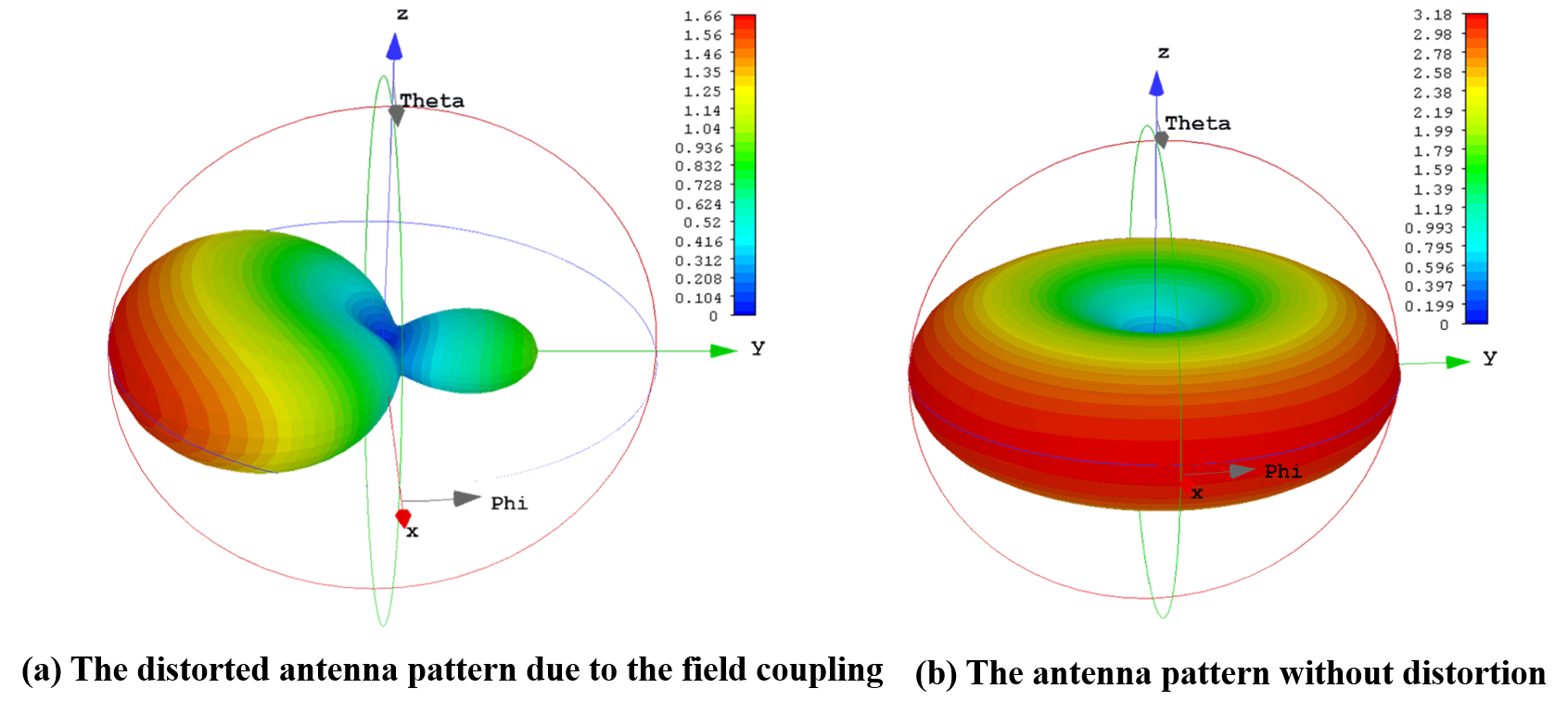
Figure 1: The antenna pattern (a) with distortion due to the field coupling, (b) without distortion.

When only one antenna is excited in the array, the distorted pattern due to the field coupling is shown in Fig. 1 (a). It can be found the pattern is irregular and far different from the antenna pattern without distortion as shown in Fig. 1 (b). According to Theorem 1, the field coupling matrix can be used to fully characterize the distortion of the radiation pattern, e.g., the difference between Fig. 1 (a) and Fig. 1 (b). The intuition is that the distorted electric field can be uniquely represented by the spherical wave coefficients $\mathbf{q}_{c_{n}}$ [17], which is also uniquely determined by the matrix $\mathbf{C}$ and the undistorted field ${\mathbf{E}}_{s}$ illustrated by Fig. 1 (b).

According to (6) and (35), the directivity factor based on the field coupling matrix is thus

$$D_{c}=\dfrac{(\mathbf{C}\mathbf{b})^{T}\mathbf{e}\mathbf{e}^{H}(\mathbf{C}\mathbf{b})^{*}}{(\mathbf{C}\mathbf{b})^{T}\mathbf{Z}(\mathbf{C}\mathbf{b})^{*}},$$ (47)

where $\mathbf{b}$ is the vector of excitation coefficients that maximizes the directivity $D_{c}$ based on our proposed method. It is observed that this equation is also in the form of Rayleigh quotient. Thus it is analogous to (18) to obtain the beamforming vector $\mathbf{b}$ as

$$\mathbf{b}=\zeta\mathbf{C}^{-1}\mathbf{Z}^{-1}\mathbf{e}^{*},$$ (48)

where $\zeta$ is a constant, which is determined by the total power constraint.

To analyze the effect of ohmic loss on the antenna array, it is assumed that the efficiency of each antenna is $\eta_{a}$. The normalized loss resistance induced antenna efficiency is[16]

$$r_{\text{loss}}=\frac{1-\eta_{a}}{\eta_{a}}.$$ (49)

Thus, the gain of the antenna array can be written as

$$G=\frac{(\mathbf{Cb})^{T}\mathbf{ee}^{H}(\mathbf{Cb})^{*}}{(\mathbf{Cb})^{T}(\mathbf{Z}+r_{\text{loss }}\mathbf{I}_{M})(\mathbf{Cb})^{*}}$$ (50)

where $\mathbf{I}_{M}$ is an identity matrix of size $M\times M$.

In practice, the electromagnetic properties of the antenna array always differs with the idealized simulations. Some practical factors, such as the manufacturing of antenna array, the influence of coaxial cable radiation, etc. will affect the radiation pattern and the directivity of the antenna array. To obtain the realistic impedance and field coupling of antenna arrays, a measurement-based coupling matrix calculation method is proposed as follows.

III-B Measurement-based computation of the superdirective beamforming vector

The essence of our proposed superdirective beamforming method is the two coupling matrices, i.e., the field coupling matrix and the impedance matrix. However, the full-space electric field data needed to calculate the two coupling matrices cannot be accessed easily like in the simulation tools. Moreover, some realistic factors may not be easily modeled in simulations. As a result, we propose a practical method to obtain the coupling matrices. This method takes the realistic factors into consideration, and the input data needed is also accessible. In the following, we will show the details of this method in the context of a compact dipole antenna array. Nevertheless, this method can be applied to other types of antennas as well. Without loss of generality, the principal radiation plane of the dipole is the H-plane ($\theta=90^{o}$) in our setting. We only use the electric field data of the H-plane to calculate the coupling matrices. Such a simplification facilitates the measurements, which can be done easily in an anechoic chamber with a rotating platform. Even with only part of the electric field data, the effectiveness of this method has been proven in simulation and practice.

First consider a z-directed dipole antenna located at the origin with current filed $\mathbf{J}$, the Green’s function to deduce the electric field radiated by this antenna is written as [20]

$$\mathbf{G}(\mathbf{r})=-j\frac{\eta}{2\lambda}\left(\mathbf{I}_{3}+\frac{1}{k^{2}}\nabla\nabla^{T}\right)\frac{\mathrm{e}^{-ik\|\mathrm{r}\|_{2}}}{\|\mathrm{r}\|_{2}},$$ (51)

where $\mathbf{I}_{3}$ is an identity matrix of size $3\times 3$, $\nabla=\left[\frac{\partial}{\partial x},\frac{\partial}{\partial y},\frac{\partial}{\partial z}\right]^{T}$ is the gradient operator, $\mathbf{r}$ is the coordinate of the far-field region. The electric field can thus be expressed as

$$\mathbf{E}(\mathbf{r})=\int_{\Omega}\mathbf{G}\left(\mathbf{r}-\mathbf{r}^{\prime}\right)\mathbf{J}\left(\mathbf{r}^{\prime}\right)\mathrm{d}\mathbf{r}^{\prime},$$ (52)

where $\Omega$ is the volume of the antenna. It can be found from (51) and (52) that when the antenna is moved to $[0,d,0]$, the variation of the radiated electric field is caused by the term $\frac{\mathrm{e}^{-ik\|\mathrm{r}\|_{2}}}{\|\mathrm{r}\|_{2}}$ of (51). The Green’s function is changed to

$$\mathbf{G}(\mathbf{\bar{r}})=-j\frac{\eta}{2\lambda}\left(\mathbf{I}_{3}+\frac{1}{k^{2}}\nabla\nabla^{T}\right)\frac{\mathrm{e}^{-ik\|\mathrm{r-d\sin\theta\sin\phi}\|_{2}}}{\|\mathrm{r-d\sin\theta\sin\phi}\|_{2}},$$ (53)

It is obvious that both the amplitude and phase of the electric field have been changed. However, since the far-field is the considered application scenario, the antenna spacing satisfies $d\ll\|\mathrm{r}\|_{2}$, which indicates that $\|\mathrm{r-d\sin\theta\sin\phi}\|_{2}\approx\|\mathrm{r}\|_{2}$. Hence, the change of far-field radiation amplitude due to the variety of antenna positions in the array is negligible, which simplifies the our measurement scheme.

Consider an uniform linear antenna array with $M$ antennas, the position of each antenna is sequentially numbered with #1, #2, $\cdots$, #$M$. The impedance coupling matrix of the antenna array, i.e., the $\mathbf{Z}$ matrix in (12), is first calculated. The specific measurement method is to first place a dipole antenna at the center of the rotating platform to measure its far-field amplitude pattern ${\Lambda_{s}}(\phi)$, where $\phi$ varies from $-180^{\circ}$ to $180^{\circ}$. Next, this antenna is placed at #1 and its phase pattern $\Psi_{s_{1}}(\phi)$ is measured. Similarly, this antenna is then placed at #2, #3, $\cdots$, #$M$, and the corresponding phase patterns $\Psi_{s_{2}}(\phi)$, $\Psi_{s_{3}}(\phi)$, $\cdots$, $\Psi_{s_{M}}(\phi)$ are measured. According to (4) and the fact that $\theta=90^{o}$, the $i$-th row and $j$-th column of the impedance coupling matrix $\mathbf{Z}$ can be calculated as

$${{z}_{ij}}=\sum\limits_{\phi}{{{(\Lambda_{s}(\phi))}^{2}}}{{e}^{j\cdot\Psi_{s_{i}}(\phi)}}{{e}^{-j\cdot\Psi_{s_{j}}(\phi)}}$$ (54)

Next, the field coupling matrix $\mathbf{C}$ of the antenna array will be calculated. First, $M$ antennas are placed at #1, #2, $\cdots$, #$M$ on the antenna mount respectively. The antenna selection vector $s_{n}$ (where the $n$-th element is 1 and the other elements are 0) is applied to excite the antenna array. To measure the amplitude pattern $\Lambda_{c_{n}}$ and phase pattern $\Psi_{c_{n}}$ of the $n$-th antenna in the array, the antenna selection vector is set to $s_{n}$. Note that the measured amplitude pattern $P_{r}(\theta,\phi)$ is the power density of electric field $E(\theta,\phi)$, and the relation between them is

$$P_{r}(\theta,\phi)=\frac{1}{2}\Re e\left[\mathbf{E}\times\mathbf{H}^{*}\right]=\frac{1}{2\eta}\left|E(\theta,\phi)\right|^{2}$$ (55)

Thus, the information of the radiated electric field can be extracted by (55), the measured amplitude pattern, and the phase pattern. The electric field of the $n$-th antenna thus is

$$\mathbf{E}_{c_{n}}(\phi)=2\eta\sqrt{\Lambda_{c_{n}}(\phi)}e^{j\cdot\Psi_{c_{n}}(\phi)}$$ (56)

Leveraging the spherical wave expansion method as described in the previous section, the spherical wave coefficients of each measured electric field are calculated. In the test, there are many factors that may cause measurement errors, such as the shake of the rotating table, the thermal noise of the test instrument, etc. However, these noises can be alleviated by an appropriate truncated constant [21]. According to the criterion $N=kr_{0}+10$, the truncated constant $N$ is set to 13 in our experiments, which is effective in practice to depict and denoise the measured electric field. Consequently, the field coupling matrix and the superdirective beamforming vector are calculated by (46) and (48). Moreover, the non-ideal factors, which affect the antenna radiation pattern, have been considered in this practical measurement scheme. It is noticeable that the coupling matrices are parameters related the geometry structure of the antenna array. Thus when the array is fabricated, we only need to measure these parameters once.

IV Numerical Results

In order to validate the effectiveness of the proposed superdirective beamforming methods, full-wave simulations and realistic experiments are carried out in this section.

IV-A Simulation Results

A printed dipole antenna array with a center frequency of 1600 MHz is designed as shown in Fig. 2, where the width and length of the dipole are $w=1\ mm$ and $l=71.5\ mm$, respectively. The dipole antenna is printed on the FR-4 substrate ($\epsilon_{r}=4.47$, $\mu_{r}=1$ , $\tan\delta=0.0027$ and the thickness is $0.8\ mm$) of size $12.2\ mm\times 78\ mm$. The transmit power is 1 W in simulations.

Figure 2: The schematic view of the printed dipole antenna array.

In conventional precoding strategies that ignore impedance coupling, the maximum ratio transmission (MRT) is considered to be the optimal beamforming vector that maximizes signal-to-noise ratio (SNR)[22]. Since the impedance coupling is not considered, the maximum directivity factor of the MRT is proportional to the number of antennas $M$. However, by exploiting the impedance coupling effect between antennas, the maximum directivity factor can be much greater. In the following simulations, we will compare the performance of our proposed superdirectivity beamforming scheme and the MRT.

The full-wave simulation results of the directivity as a function of the antenna spacing are illustrated in Fig. 3, for the case of $M=3$. In this figure, the theoretical directivity is calculated by (47) and (48). It can be found that the maximum theoretical directivity increases with the decreasing of the antenna spacing, and the directivity reaches $11.2$ when the spacing is $0.1\lambda$. When the antenna array is directly excited by the beamforming vector calculated by (18), the directivity factor also increases at first as the spacing decreases, yet reaches a maximum around $0.23\lambda$. Afterwards, it starts to decrease with smaller spacing. This is because the smaller the spacing, the greater the field coupling between the antennas and the more pronounced the side effects of the traditional method, which does not take the field coupling into account. However, our proposed double-coupling based method has obvious gains and the directivity of the antenna array is in line with the theoretical value. The maximum directivity of MRT is obtained after the array is excited by $\mathbf{e}^{*}$ calculated by (8) in full-wave simulation software, and It can be seen that the directivity of the MRT is consistently smaller than that of the proposed method or even the traditional method for antenna spacing less than $0.5\lambda$. When the spacing is around $0.5\lambda$, it can be found that the four curves almost overlap, which is because the coupling effects can be ignored under such antenna spacing.

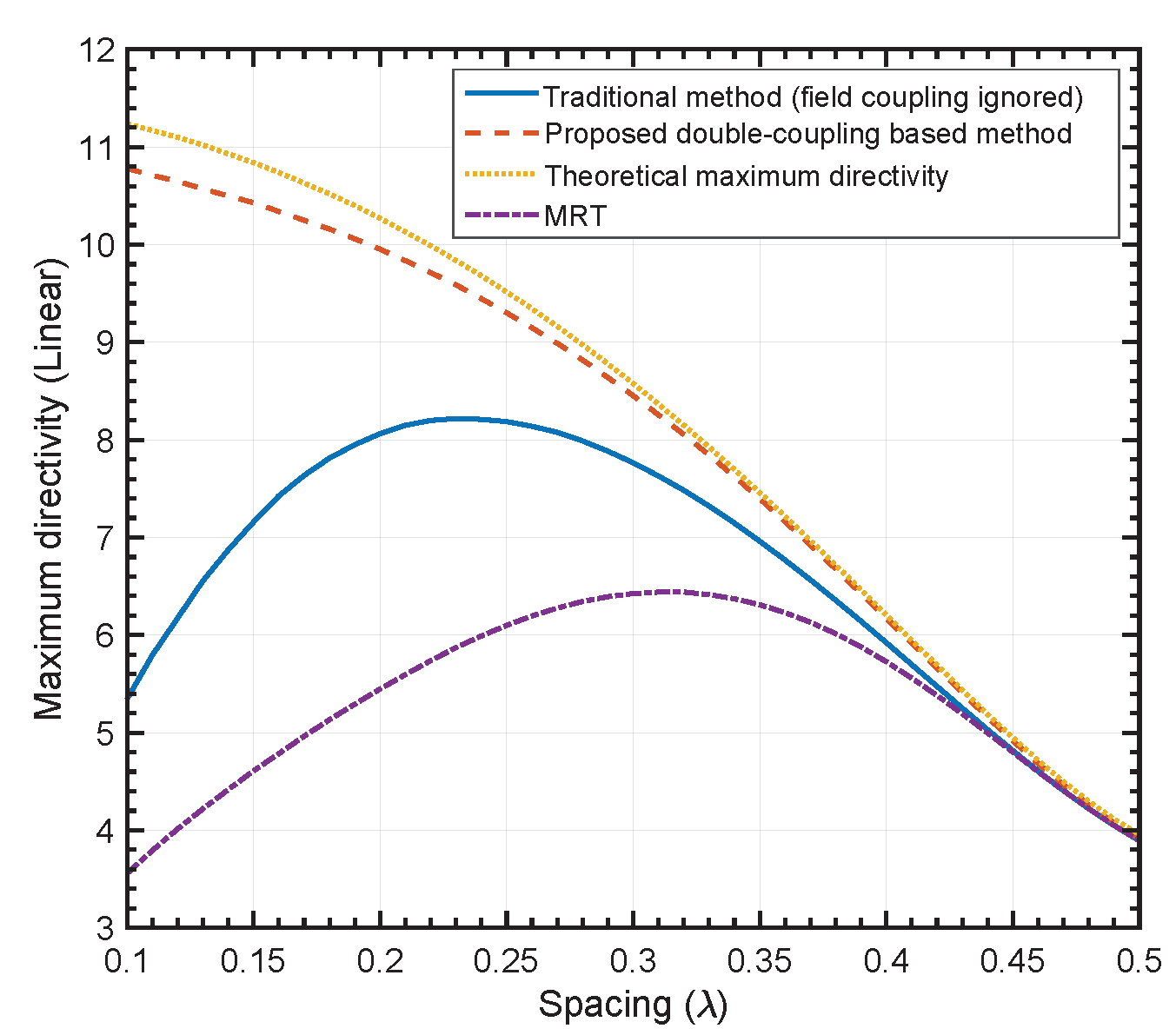
Figure 3: The maximum directivity of three-element dipole antenna array.

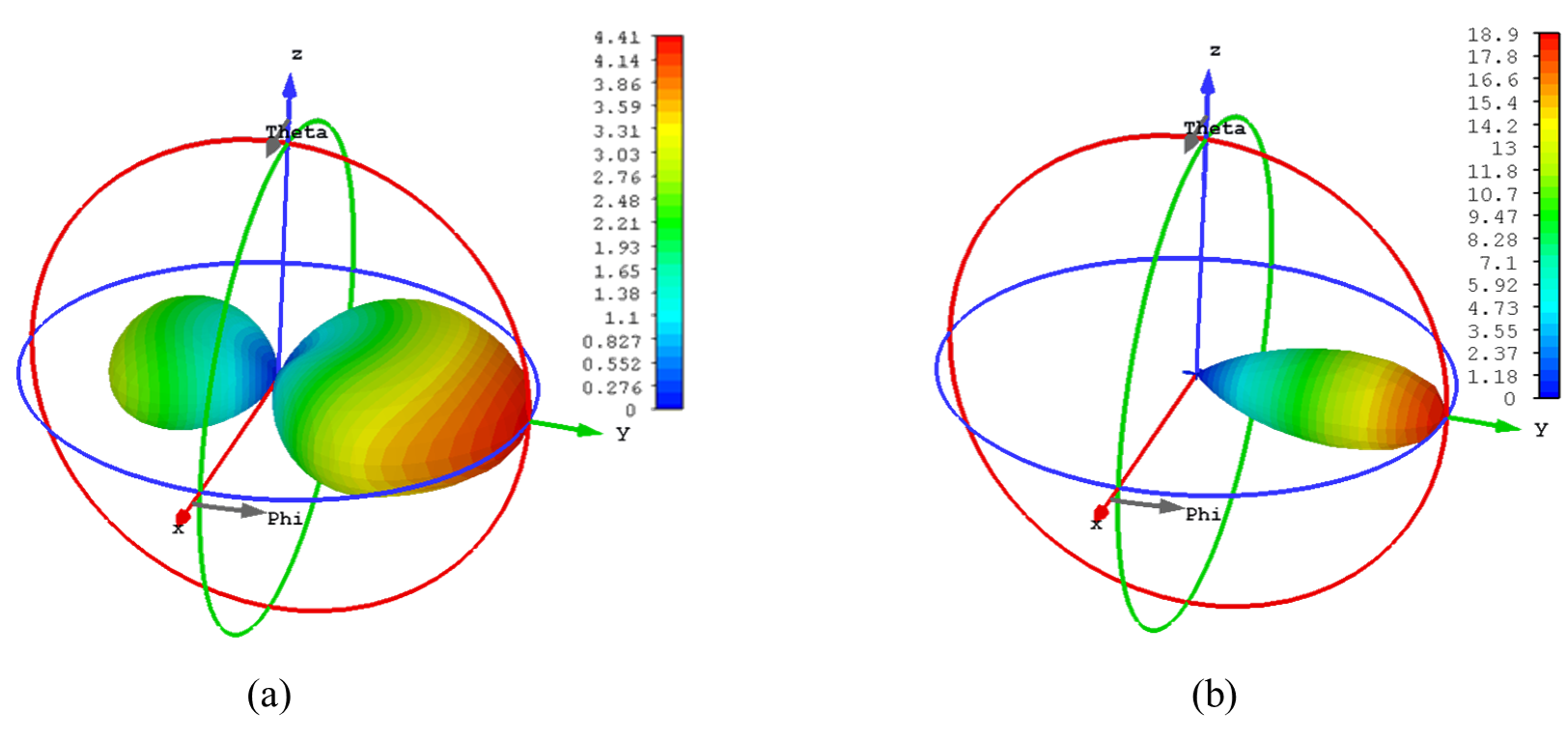
Figure 4: The radiation patterns of the linear dipole antenna arrays, where $M=4$, $d=0.1\lambda$. (a) Excited by traditional superdirective beamforming method. (b) Excited by the proposed method.

Fig. 4 shows the 3D directivity pattern of the linear dipole array with four antennas. The antenna spacing is 0.1$\lambda$. Fig. 4 (a) and Fig. 4 (b) are the patterns when the beamforming vector is calculated by the traditional method that ignores the field coupling and by our proposed double-coupling based method respectively. Compared with Fig. 4 (a), it is evident that the radiated pattern is narrower and the back lobe is smaller in Fig. 4 (b). It can be seen that the directivity factor of the traditional method is only 3.4, while the theoretical value is 18.9, which is much larger. When the proposed beamforming method is applied, the directivity is close to the theoretical value.

Fig. 5 shows the directivities for a four-dipole antenna array. It can be seen that the directivity based on the traditional method has a poor performance in the small spacing region, while our proposed method is close to the theoretical values.

Figure 5: The performances of achieved maximum directivity with four dipole antennas.

Some specific values are shown in Table I. Notice that the theoretical value is greater than $M^{2}$, which is because dipole antennas are used instead of isotropic antennas[9].

TABLE I: The directivity(power/power)

$M$	$d$	MRT	Traditional method	Proposed method	$M^{2}$
3	0.1$\lambda$	3.557	5.343	10.78	9
	0.2$\lambda$	5.448	8.064	9.953	9
4	0.1$\lambda$	4.533	4.362	18.88	16
	0.2$\lambda$	7.012	9.312	16.64	16

To analyze the impact of ohmic loss on the performance of directivity, the gain of the antenna array with different spacing is illustrated in Fig. 6. When the number of antennas is 2 and 4 respectively, the radiation efficiency of the antenna is 96%. It can be found the gain does not keep increasing as the antenna spacing decreases, and the larger the number of antennas, the more obvious the effect of ohmic loss at smaller spacing. Consequently, the maximum gain is 9.6 when the number of antennas is 4 and the spacing is 0.33$\lambda$. This phenomenon can be explained mathematically by (50), where the impedance matrix $\mathbf{Z}$ converges to a singular matrix as the antenna spacing tends to zero. However, in this case, the singularity of the impedance matrix changes when a small ohmic loss $r_{\text{loss}}$ exists, which impairs the antenna array gain significantly. Nevertheless, the problem of ohmic loss can be alleviated by high-temperature superconducting antennas [23].

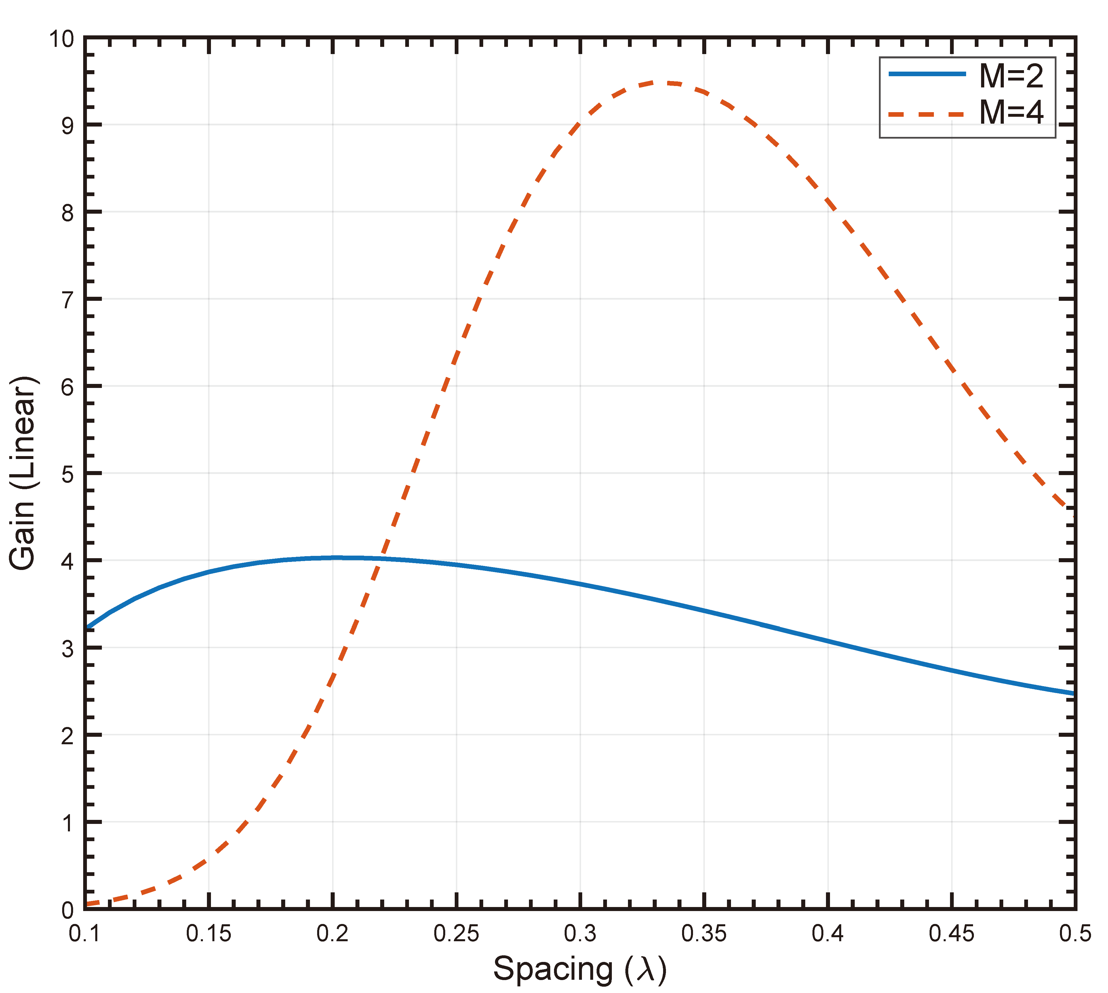
Figure 6: The gain achieved by the proposed method in the presence of the ohmic loss.

IV-B Experimental Results

To validate the proposed beamforming method in practice, we design and fabricate a prototype of the superdirective antenna array. The Printed Circuit Board (PCB) dipole is selected as the radiating element of the array, and its parameters are consistent with the simulation settings. Each antenna is connected to a coaxial feed line with a SubMiniature version A (SMA) connector.

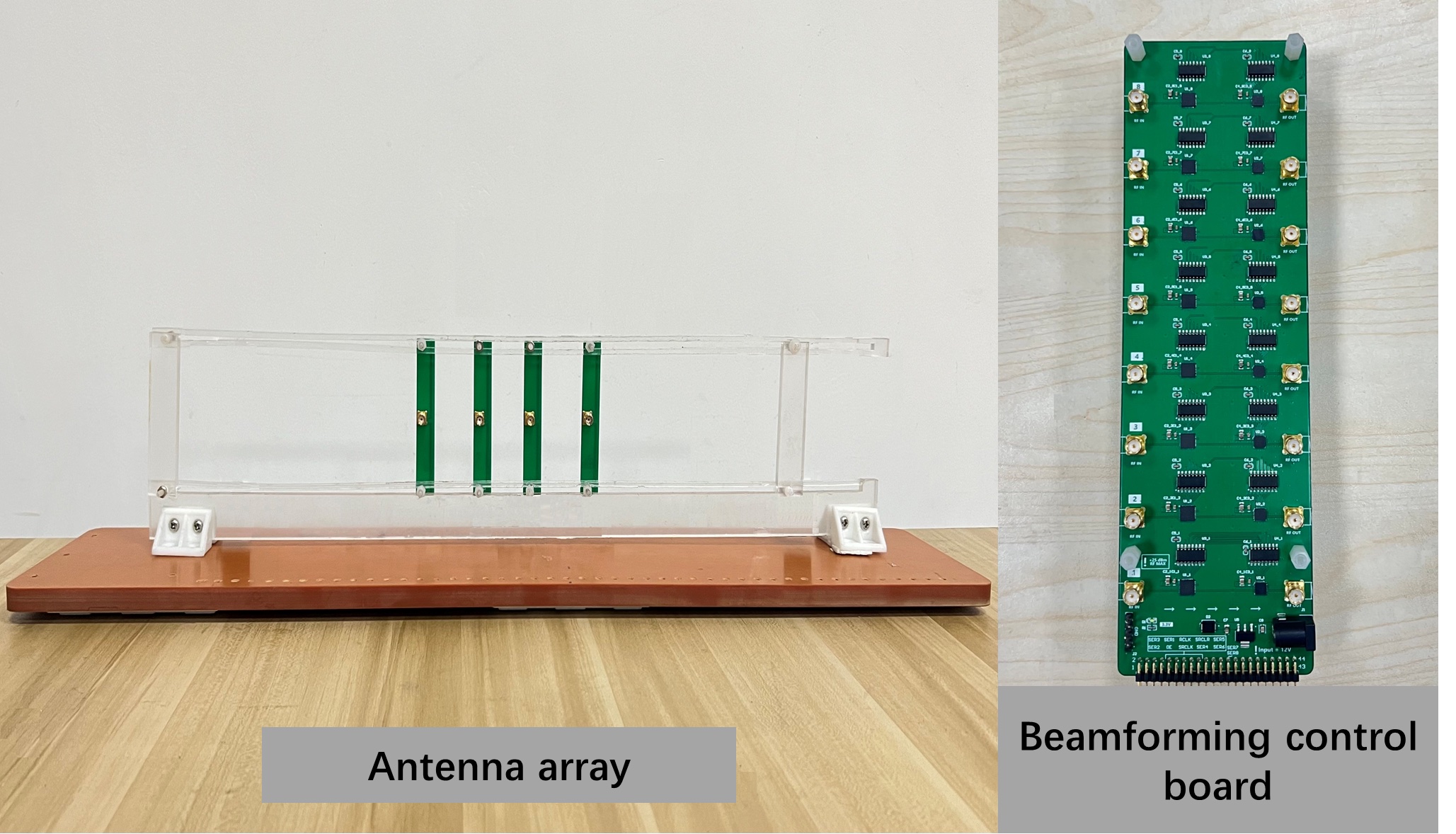
Figure 7: The designed antenna array and beamforming control board.

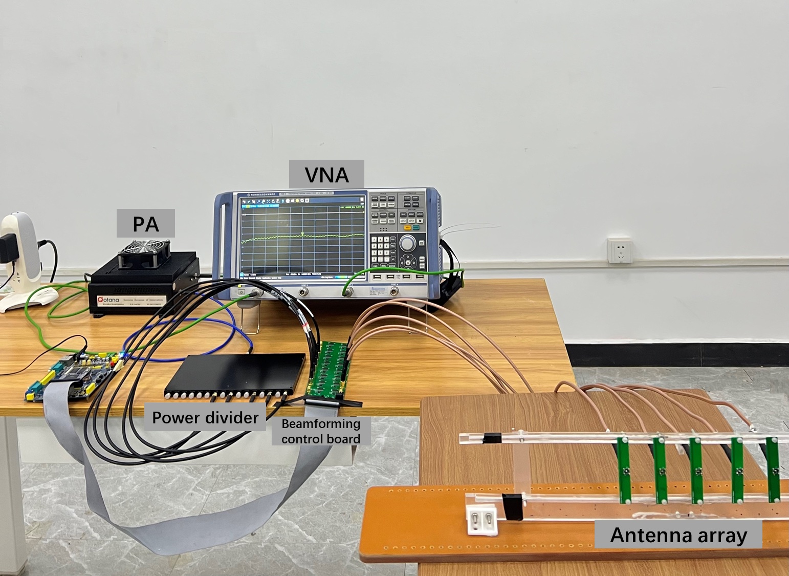
Figure 8: The hardware platform of the superdirective antenna array testing system.

Figure 9: The microwave anechoic chamber of size 4 m × 6 m × 4 m. The Array-RX antenna distance is 4.8 m.

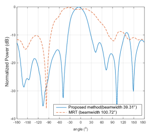
(a) Comparing with MRT.

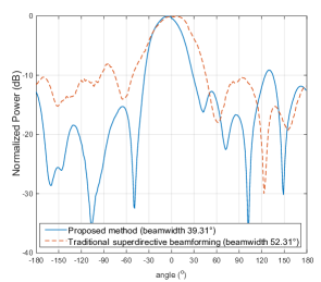
(b) Comparing with the traditional superdirective beamforming method.

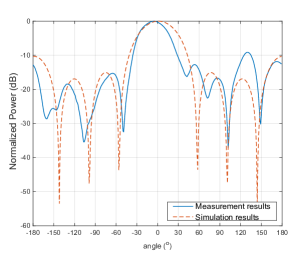
(c) Comparing with the simulation results.

Figure 10: The measured normalized power of the proposed beamforming method in principal radiation plane ($\theta=90^{o}$) comparing with (a) the MRT, (b) the traditional superdirective beamforming method (field coupling ignored) and (c) the full-wave simulation results. The number of antennas is 4 and the antenna spacing is 0.2$\lambda$.

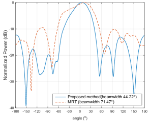
(a) Comparing with MRT.

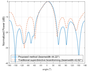
(b) Comparing with the traditional superdirective beamforming method.

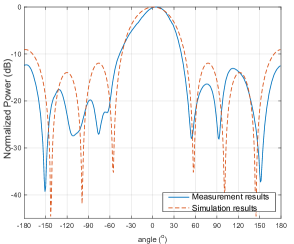
(c) Comparing with the simulation results.

Figure 11: The measured normalized power in the principal radiation plane ($\theta=90^{o}$) with 4 dipole antennas and an antenna spacing of 0.3$\lambda$.

In order to excite each antenna with software-controlled phase and amplitude, we develop a beamforming control board that has 8 channels, and the beamforming coefficient for each channel is quantized to 8 bits in phase and 7 bits in amplitude. The fabricated antenna array and beamforming control board are show in Fig. 7. A 16-way power divider is utilized to extend the RF signal and its output is connected to the input of the beamforming control board. The antenna array to be measured is connected to the output of the beamforming control board. The initial phase differences between the channels are measured by the vector network analyzer (VNA) and calibrated by the beamforming control board. The diagram of the hardware system is shown in Fig. 8.

The experiments are carried out in the microwave anechoic chamber, as shown in Fig. 9. The tested antenna array is fixed to the center pillar of the rotating platform, and the receiving antenna has the same height as the transmitting antenna array. The distance between the antenna array and receive antenna is 4.8 m, which satisfies the far-field test requirement.

In the experiments, we use a VNA to measure the far-field amplitude and phase of the antenna under test (AUT), where the VNA model is R&S ZNB. Specifically, the antenna array is connected to the output port of the beamforming control board, whose input port is linked to the power divider. The input of the power divider is connected to port one of the VNA, and the receiving antenna is connected to port two. The radiation field information of the AUT can thus be obtained by measuring the S21 parameter from the VNA.

We compare our proposed beamforming method with the MRT, the traditional superdirective beamforming method (field coupling ignored), and the simulation results. Fig. 10 shows the corresponding results when the number of antennas is four and the antenna spacing is $0.2\lambda$. It can be found that the MRT method has the widest 3-dB beamwidth, which equals ${\rm 100.72}^{\circ}$, in the direction of interest. However, the narrowest 3-dB beamwidth, which equals 39.31^∘, is achieved by our proposed beamforming method. From Fig. 10 (b), we may observe that although the traditional superdirective beamforming method also has a narrower 3-dB beamwidth compared to the MRT, its power level is higher than our method in almost all directions other than the main lobe. It can be found from Fig. 10 (c) that a good agreement is attained in both the main lobe and the side lobes, except the region around 120^∘. The asymmetry of the measurement results may be attributed to the coaxial lines connected to the antennas on one side.

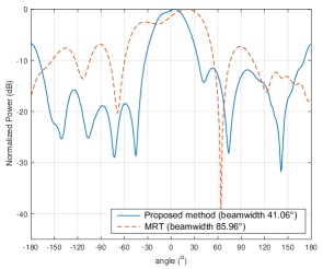
(a) Comparing with the maximum ratio transmission

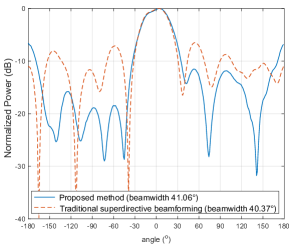
(b) Comparing with the traditional superdirective beamforming method

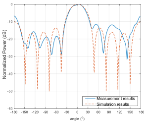
(c) Comparing with the simulation results

Figure 12: The measured normalized power in the principal radiation plane ($\theta=90^{o}$) with 5 dipole antennas and an antenna spacing of 0.3$\lambda$.

Then, the number of antennas is maintained while the spacing is changed to ${\rm 0.3}\lambda$. The measurement results are shown in Fig. 11. It can be found in Fig. 11 (a) that the 3-dB beamwidth of the MRT is ${\rm 71.24^{\circ}}$, which is better than the case that the spacing is $0.2\lambda$. The phenomenon is due to the weaker coupling effects between antennas, which is more preferable for the MRT. In Fig. 11 (b), the 3-dB beamwidth of our method and the traditional method is similar, yet our method still performs well in sidelobe suppression. Compared to the case with antenna spacing of $0.2\lambda$, the 3-dB beamwidth of our method increases while the traditional method decreases. The results are in conformity with the theory that the directivity increases with smaller antenna spacing. Since the field coupling is ignored, the directivity of the traditional method is crippled in the small spacing regions. Fig. 11 (c) shows that there is also a good agreement between the measurement and the simulation when the antenna spacing is $0.3\lambda$.

To validate the generality of our method, we add one more antenna into the array and keep the spacing unchanged. The measurement results are shown in Fig. 12. As we may observe, our proposed method still performs best among all beamforming methods while in line with the simulation results, and thus its effectiveness to achieve superdirectivity in practice is proved.

In order to quantify the measurement results, the principal plane ($\theta=90^{\circ}$) directivity $D_{p}$ is defined analogously to the definition of directivity as

$$D_{p}\triangleq\frac{\max\{\Lambda(\phi),\phi\in[-180^{\circ},180^{\circ})\}}{\frac{1}{L}\sum_{\phi}\Lambda(\phi)}$$ (57)

where $L$ is the number of sample points in the principal radiation plane. Based on (57), the calculated principal plane directivity results of each array under different conditions are shown in Table II, where $M$ is the number of antennas and $d$ is the antenna spacing. It can be found that our proposed method outperforms other beamforming methods significantly.

TABLE II: The principle plane directivity (power/power)

$M$	$d$	MRT	Traditional method	Proposed method
4	$0.2\lambda$	3.1290	4.9441	7.3273
	$0.3\lambda$	4.3273	5.4899	6.443
5	$0.3\lambda$	4.0398	5.7636	6.9878

V Conclusion

In this paper, we addressed the problem of beamforming coefficient calculation for superdirective antenna arrays. A double coupling-based scheme was proposed, where the antenna coupling effects are decomposed to impedance coupling and field coupling, which is obtained by a proposed spherical wave expansion method. We proved the uniqueness of the obtained solution, which is able to fully characterize the distorted coupling field. Such a method is applicable in both electromagnetic simulation and practice (after the proposed adaptations). Moreover, our methodology can be scaled up with more antennas and applied to other topologies, such as 16-elements array, 32-elements array, and planar arrays. We also developed a prototype of the superdirective dipole antenna array working at 1600 MHz and a hardware experimental platform in order to validate the proposed methods. The simulation results and experimental measurements both showed that our proposed method outperforms the state-of-the-art methods.

Appendix A Proof of Theorem 1

The electric field radiated by the $z$-diretcted dipole antenna located at the origin can be expressed as[24]

$$\mathbf{e(r)}=j\eta\frac{kI_{0}le^{-jkr}}{4\pi r}\sin\theta\hat{\theta},$$ (58)

where $\mathbf{r}=[r\sin\theta\cos\phi,r\sin\theta\sin\phi,r\cos\theta]$ is the far-field coordinate, $r=\|\mathbf{r}\|_{2}$ is the radius distance, $\hat{\theta}$ is the unit vector of $\theta$-direction. The field can be expanded with the spherical wave expansion method as

$$\mathbf{e(r)}=-jk\sqrt{\eta}\frac{e^{-jkr}}{4\pi r}\sqrt{\frac{3}{4}}Q_{2,0,1}(\sin\theta)\hat{\theta}.$$ (59)

It can be found that the field has only one expansion coefficient $Q_{2,0,1}$ , i.e., the dipole antenna is a single-mode antenna. Thus there is no complicated modes coupling between the antennas to affect their respective radiation field [25][26]. Without loss of generality, $M$ dipole antennas are evenly distributed at the positive half axis of z-axis, and the first antenna is at the origin. Therefore, the electric field radiated by the $m$-th antenna is

$$\mathbf{e}(\mathbf{r}_{m})=$$

$$\quad-jk\sqrt{\eta}\frac{e^{-jk(r-(m-1)d\sin\theta\sin\phi)}}{4\pi(r-(m-1)d\sin\theta\sin\phi)}\sqrt{\frac{3}{4}}Q_{2,0,1}(\sin\theta)\hat{\theta}.$$ (60)

Since $r\gg d$, we have $r-(m-1)d\sin\theta\sin\phi\approx r$. Thus, Eq. (A) can be rewritten as

$$\mathbf{e}(\mathbf{r}_{m})=$$

$$\quad-jk\sqrt{\eta}\frac{e^{-jk(r-(m-1)d\sin\theta\sin\phi)}}{4\pi r}\sqrt{\frac{3}{4}}Q_{2,0,1}(\sin\theta)\hat{\theta}.$$ (61)

Letting $\mathbf{E}$ be the function group of the electric field radiated by antennas located at different positions, i.e.,

$$\mathbf{E}=\{\mathbf{e}(\mathbf{r}_{1}),\,\mathbf{e}(\mathbf{r}_{2}),\,\cdots,\,\mathbf{e}(\mathbf{r}_{M})\}.$$ (62)

We will prove that $\mathbf{E}$ is a group of linearly independent functions. It is notable that $\mathbf{e}(\mathbf{r}_{m})$ is a function with two variables $\theta$ and $\phi$. The equation (62) can be rewritten as

$$\mathbf{e}(\mathbf{r}_{m})=Ae^{jk(m-1)d\sin\phi\sin\theta}\sin\theta\hat{\theta}$$ (63)

and

$$A=-jk\sqrt{\eta}\frac{e^{-jkr}}{4\pi r}\sqrt{\frac{3}{4}}Q_{2,0,1}.$$ (64)

Assuming that there exists a series of constants $k_{i},i=1,\cdots,M$ such that

$$k_{1}\mathbf{e}(\mathbf{r}_{1})+k_{2}\mathbf{e}(\mathbf{r}_{2})+\cdots+k_{M}\mathbf{e}(\mathbf{r}_{M})=0.$$ (65)

We want to show that the coefficients $k_{i},i=1,\cdots,M$ are all zero. Differentiating the equation (65) with respect to $\sin\phi$, we obtain

$$k_{2}(jkd\sin\theta)\mathbf{e}(\mathbf{r}_{2})+\cdots+k_{M}(jk(M-1)d\sin\theta)\mathbf{e}(\mathbf{r}_{M})=0.$$ (66)

Continuing differentiating the above equation $(M-2)$ times with respect to $\sin\phi$ yields

$$k_{M}(jk(M-1)d\sin\theta)^{M-1}\mathbf{e}(\mathbf{r}_{M})=0,$$ (67)

which implicates that $k_{M}=0$. By backtracking the process we can obtain that $k_{i}=0,i=1,\cdots,M$. Thus, $\mathbf{E}$ is a group of linearly independent functions. Without loss of generality, take the calculation of the first column of the coupling matrix as an example. According to the one-to-one relationship between the electric field and the spherical wave coefficients [17], the coefficient vector of the antenna located at different positions as

$$\mathbf{Q}_{s}=\{\mathbf{q}_{{s}_{1}},\mathbf{q}_{{s}_{2}},\cdots,\mathbf{q}_{{s}_{M}}\},$$ (68)

is also the group of linearly independent vectors. And the coupling field is radiated by these antennas together, i.e. $\mathbf{q}_{{c}_{1}}\in{\rm span}\{\mathbf{q}_{{s}_{n}}:n\in[1,M]\}$. Since ${\rm rank}(\mathbf{Q}_{s})={\rm rank}(\mathbf{Q}_{s}|\mathbf{q}_{{c}_{1}})$, the linear function

$$\mathbf{q}_{{c}_{1}}=c_{11}\mathbf{q}_{{s}_{1}}+c_{21}\mathbf{q}_{{s}_{2}}+\cdots+c_{M1}\mathbf{q}_{{s}_{M}}$$ (69)

has a unique solution[27].

The distorted field ${\mathbf{e}}_{c_{n}},n\in\left[1,M\right]$ can be uniquely represented by the spherical wave coefficients $\mathbf{q}_{c_{n}}$. Since $\mathbf{q}_{c_{n}}$ is uniquely determined by the field coupling matrix $\mathbf{C}$ and the electric field without distortion (or the corresponding spherical wave coefficients $\mathbf{q}_{s_{n}},n=1,\cdots,M$), the radiation pattern distortion can thus be fully characterized by $\mathbf{C}$. $\hfill\qed$.

References

- [1] L. Han, H. Yin, and T. L. Marzetta, “Coupling matrix-based beamforming for superdirective antenna arrays,” in IEEE Int. Conf. Commun. (IEEE ICC), Seoul, South Korea, May, 2022.
- [2] T. L. Marzetta, E. G. Larsson, H. Yang, and H. Q. Ngo, Fundamentals of Massive MIMO. Cambridge University Press, 2016.
- [3] T. L. Marzetta, “Noncooperative cellular wireless with unlimited numbers of base station antennas,” IEEE Trans. Wireless Commun., vol. 9, no. 11, pp. 3590–3600, 2010.
- [4] E. Björnson, L. Sanguinetti, H. Wymeersch, J. Hoydis, and T. L. Marzetta, “Massive MIMO is a reality—what is next five promising research directions for antenna arrays,” Digit. Signal Process., vol. 94, pp. 3–20, 2019.
- [5] A. Pizzo, L. Sanguinetti, and T. L. Marzetta, “Fourier plane-wave series expansion for holographic mimo communications,” IEEE Trans. Wireless Commun., vol. 21, no. 9, pp. 6890–6905, 2022.
- [6] A. Pizzo, T. L. Marzetta, and L. Sanguinetti, “Spatially-stationary model for holographic MIMO small-scale fading,” IEEE J. Sel. Areas Commun., vol. 38, no. 9, pp. 1964–1979, 2020.
- [7] P. C. Clemmow, The plane wave spectrum representation of electromagnetic fields: International series of monographs in electromagnetic waves. Elsevier, 2013.
- [8] T. B. Hansen, “Exact plane-wave expansion with directional spectrum: Application to transmitting and receiving antennas,” IEEE Trans. Antennas Propag., vol. 62, no. 8, pp. 4187–4198, 2014.
- [9] E. E. Altshuler, T. H. O’Donnell, A. D. Yaghjian, and S. R. Best, “A monopole superdirective array,” IEEE Trans. Antennas Propag., vol. 53, no. 8, pp. 2653–2661, 2005.
- [10] L. Sanguinetti, E. Björnson, and J. Hoydis, “Toward massive MIMO 2.0: Understanding spatial correlation, interference suppression, and pilot contamination,” IEEE Trans. Commun., vol. 68, no. 1, pp. 232–257, 2020.
- [11] A. Bloch, R. Medhurst, and S. Pool, “A new approach to the design of super-directive aerial arrays,” Proc. IEE, Pt. III, vol. 100, no. 67, pp. 303–314, 1953.
- [12] A. Uzkov, “An approach to the problem of optimum directive antenna design,” in Comptes Rendus (Doklady) de l’Academie des Sciences de l’URSS, vol. 53, no. 1, 1946, pp. 35–38.
- [13] T. L. Marzetta, “Super-directive antenna arrays: Fundamentals and new perspectives,” in 53rd Asilomar Conf. Signals Syst Comput., ACSCC 2019, Pacific Grove, CA, USA, November, 2019.
- [14] C. Volmer, M. Sengul, J. Weber, R. Stephan, and M. A. Hein, “Broadband decoupling and matching of a superdirective two-port antenna array,” IEEE Antennas Wirel. Propag. Lett., vol. 7, pp. 613–616, 2008.
- [15] A. Clemente, M. Pigeon, L. Rudant, and C. Delaveaud, “Design of a super directive four-element compact antenna array using spherical wave expansion,” IEEE Trans. Antennas Propag., vol. 63, no. 11, pp. 4715–4722, 2015.
- [16] R. E. Collin, Antenna theory Part 1, F. J. Zucker, Ed. New York: New York, 1969.
- [17] J. Hald and F. Jensen, Spherical near-field antenna measurements. Iet, 1988, vol. 26.
- [18] K. Belmkaddem, T. P. Vuong, and L. Rudant, “Analysis of open-slot antenna radiation pattern using spherical wave expansion,” IET Microw. Antennas Propag., vol. 9, no. 13, pp. 1407–1411, 2015.
- [19] S. Sadat, C. Ghobadi, and J. Nourinia, “Mutual coupling compensation in small phased array antennas,” in IEEE Antennas Propag. Soc. Int. Symp., 2004., vol. 4, 2004, pp. 4128–4131 Vol.4.
- [20] R. F. Harrington, Time-harmonic electromagnetic fields, ser. IEEE Press series on electromagnetic wave theory. New York: IEEE Press : Wiley-Interscience, 2001.
- [21] P. Koivisto, “Reduction of errors in antenna radiation patterns using optimally truncated spherical wave expansion,” Progress In Electromagnetics Research, vol. 47, pp. 313–333, 2004.
- [22] D. G. Brennan, “Linear diversity combining techniques,” Proceedings of the IRE, vol. 47, no. 6, pp. 1075–1102, 1959.
- [23] R. C. Hansen and R. E. Collin, Small antenna handbook. Wiley Online Library, 2011.
- [24] C. A. Balanis, Antenna theory: analysis and design. John wiley & sons, 2015.
- [25] T. Bird, “Mutual coupling in arrays of coaxial waveguides and horns,” IEEE Trans. Antennas Propag., vol. 52, no. 3, pp. 821–829, 2004.
- [26] S. Lou, B. Duan, W. Wang, C. Ge, and S. Qian, “Analysis of finite antenna arrays using the characteristic modes of isolated radiating elements,” IEEE Trans. Antennas Propag., vol. 67, no. 3, pp. 1582–1589, 2018.
- [27] W. H. Greub, Linear algebra. Springer Science & Business Media, 2012, vol. 23.