Sterile versus prolific individuals pertaining to linear-fractional Bienaymé-Galton-Watson trees

Abstract.

In a Bienaymé-Galton-Watson process for which there is a positive probability for individuals of having no offspring, there is a subtle balance and dependence between the sterile nodes (the dead nodes or leaves) and the prolific ones (the productive nodes) both at and up to the current generation. We explore the many facets of this problem, especially in the context of an exactly solvable linear-fractional branching mechanism at all generation. Eased asymptotic issues are investigated. Relation of this special branching process to skip-free to the left and simple random walks’ excursions is then investigated. Mutual statistical information on their shapes can be learnt from this association.

Keywords: Bienyamé-Galton-Watson process, iterated linear fractional generating functions, sterile vs prolific individuals, limit laws, criticality, conditionings, fixed points, random walks (skip-free and simple).

AMS classification: 60J (60J80, 60J15).

^∗ corresponding author

1. Introduction and summary of the results

Bienaymé-Galton-Watson (BGW) branching processes have for long been a milestone in the understanding of multiplicative cascade phenomena [Good (1949) and Otter (1949)], starting with the extinction of family names in population dynamics, in the second half of the 19-th century. See [Kendall, (1966) and Jagers, (2020)] for historical background. BGW processes also appear as crude models for the spread of rumors, gravitational clustering [Sheth, (1996)], cosmic-ray cascades and the proliferation of free neutrons in nuclear fission, [Harris, (1963)].

In a BGW branching tree process for which (our background hypothesis throughout this paper):

(i) there is a positive probability for individuals of having no offspring,

(ii) the offspring number has all its moments,

there is a subtle balance and dependence between the present (the state of the population at some current generation) and the past (for example the cumulated number of nodes before this current generation). In both cases, the population, as a tree, can be split into two main types of individuals: the sterile (the dead leaves) and the prolific ones (the living nodes), both at and up to the currently observed generation number. Specific interest into these two types of individuals goes back at least to [Rényi, (1959)].

By making extensive use of the apparatus of iterated generating functions, we explore the balance and dependence between the two. We consider the many facets of this problem, especially in the context of the linear-fractional (LF) branching mechanism (obeying (i)(ii)), leading to explicit computations at all generation as a result of the stability of LF transformations under composition. Such explicit results, although being specific, illuminate the known asymptotic results concerning more general branching processes, and, on the other hand, may bring insight into less investigated aspects of the theory of branching processes. In places, we will then make allusions to other important branching mechanisms. Depending on the BGW process being (sub-)critical, supercritical, or nearly supercritical, asymptotic issues are investigated when the generation number goes to infinity. This is part of a general program of understanding on how the full past interact with the present in a BGW process. The organization of the paper is as follows:

- Section $2$: We recall some basics on the current population size of BGW processes satisfying (i)(ii), including some well-known limit laws, conditions of criticality and conditionings on criticalities. BGW processes with two-parameters LF branching mechanisms were used in the extinction of family names problem, [Steffenson, (1930, 1933)]; they deserve specific interest being an exactly solvable model. The discrete LF BGW process is indeed an important particular case being amenable to explicit computations, including - the one of its extinction probability,- the one of the important fixed point parameter $\tau$ defined in (11) and used in the conditioning of non-critical BGW processes to critical ones and in the law of the total progeny - the one of its $n$-step transition matrix leading to a tractable potential theory - the exact expression of a Kolmogorov constant - an explicit limit law of the $Q$-process. It is furthermore embeddable in a continuous-time binary BGW process. We mention a Harris derivation of its ‘stationary distribution’ [Harris, 1963]. We derive the joint law of the sterile versus prolific individuals at a current generation $n$.

- Section $3$: We are concerned with the interaction between the past and the present of BGW processes, starting with the total progeny of one or more founders (forests of trees).

The analysis of the total progeny marginal is first introduced in Section 3.1 and developed in Section 3.5. Section 3.6 considers the critical case.

We next derive a general recurrence for the joint law of the sterile and prolific individuals at and up to generation $n$, starting from a single founder; see (29) of Section 3.2. We particularize this recurrence to study:

- the joint law of the cumulated number of sterile against the cumulated number of prolific individuals in the BGW tree. This is introduced in Section 3.3 and developed in Section 3.7.

- the joint law of the cumulated number of sterile against the current number of prolific individuals in the BGW tree; see Section 3.4. We show through a simple example that answering the question: do the number of ever dead in a population outnumber or not the currently living is a delicate question that can be answered positively or negatively in the LF case, depending on the range of its two parameters.

- the joint law of the total number of leaves (sterile individuals) against the total progeny, obtaining the limiting large deviation function in Section 3.7.

- Section $4$: Two relations of BGW processes to random walks (RW’s) are next investigated. The first concerns general skip-free to the left RW’s related to BGW processes through a discrete version of the Lamperti time-change theorem known for continuous-state branching processes, [Lamperti, (1967)]. It connects the full past and the present of BGW processes. Making use of the scale function [Marchal, (2001)], we derive the law of the maximum (width) of a BGW till its first extinction, concomitantly with the law of the supremum of the RW till its first hitting time of $0$. Both are jointly finite (or not) depending on the criticality (or not) of the BGW process. We derive an explicit computation in the LF and binary fission cases.

The second concerns simple random walks (SRW’s) with nearest-neighbours moves. We revisit and highlight the Harris construction of a geometric BGW tree nested inside a SRW excursion with no holding probability, [Harris, 1952]. A node of the tree at some height $h-1$ branches when it reveals minima of the SRW at $h$. We propose an extension of this construction to SRW’s with holding probabilities (whose sample paths shows highlands and valleys), the nested tree having now a LF branching mechanism. This relation allows to derive useful mutual information on both the tree and the random walk: in particular, we show that the first hitting time of the SRW is approximately twice the total progeny of its nested tree whose time to extinction is approximately the height of the SRW. The width of the nested BGW process is the largest size of the SRW valleys.

2. Generalities on Bienaymé-Galton-Watson (BGW) branching processes

We start with generalities on such BGW processes, avoiding the case displaying finite-time explosion [Sagitov and Lindo (2015)].

2.1. Current population size: the probability generating function (p.g.f.) approach

Consider a discrete-time BGW branching process [Harris (1963); Athreya and Ney (1972)] whose reproduction law is given by the probability law $\mathbf{P}\left(M=m\right)=:\pi_{m}$, $m\geq 0$ for the number $M$ of offspring per capita. At each generation, each individual $i$ alive, independently of another, generates $M_{i}$ offspring, with $M_{i}\overset{d}{=}M$ (in distribution). Unless specified otherwise, we assume $\pi_{0}>0$ so that the process can go extinct. We let $\phi\left(z\right)=\mathbf{E}\left(z^{M}\right)=\sum_{m\geq 0}\pi_{m}z^{m}$ be the p.g.f. of $M$, so with $\phi\left(1\right)=1$ and $\phi\left(z\right)$ has convergence radius $z_{*}\in\left(1,\infty\right]$ ($M$ has all its moments finite and geometric tails). In such cases, $\phi\left(z\right)$ is analytic in the open disk $\left|z\right|<z_{*}$ of the complex plane. The latter assumptions also guarantee the existence of two real fixed points to the equation $\phi\left(z\right)=z$, one of which being $1$ (a double fixed point if $\phi\left(1\right)=\phi^{\prime}\left(1\right)=1$).

BGW processes are therefore primarily concerned with asexual organisms who die while giving birth. As such, BGW processes are birth and death Markov processes with non-overlapping generations. However, an individual dying while giving birth to a single offspring, so with probability (w.p.) $\pi_{1}$, can also be interpreted as an individual whose lifetime is delayed by one unit, thereby generating overlapping generations. According to this new interpretation, each individual $i$ of a BGW of some generation may equivalently (in law) be considered as splitting after a geometric lifetime with success probability $1-\pi_{1}$ while giving birth to $M_{i}$ offspring, given $M_{i}\neq 1$.

With $N_{n}\left(1\right)$ the number of individuals alive at generation $n$ given $N_{0}\left(1\right)=1$, we have

$$\phi_{n}\left(z\right):=\mathbf{E}\left(z^{N_{n}\left(1\right)}\right)=\phi^{\circ n}\left(z\right),$$

where $\phi^{\circ n}\left(z\right)$ is the $n$-th composition of $\phi\left(z\right)$ with itself, . Equivalently, $\phi_{n}\left(z\right)$ obeys (as from a recursion from the root) the branching property

(1) $$\phi_{n+1}\left(z\right)=\phi\left(\phi_{n}\left(z\right)\right)=\phi_{n}\left(\phi\left(z\right)\right)\text{, }\phi_{0}\left(z\right)=z.$$

Similarly, if $N_{n}\left(i\right)$ is the number of individuals alive at generation $n$ given there are $N_{0}=i$ independent founders, we clearly get

(2) $$\mathbf{E}\left(z^{N_{n}\left(i\right)}\right):=\mathbf{E}\left(z^{N_{n}}\mid N_{0}=i\right)=\phi_{n}\left(z\right)^{i}.$$

We shall also let

(3) $$\tau_{i,j}=\inf\left(n\geq 1:N_{n}=j\mid N_{0}=i\right),$$

the first hitting time of state $j\neq i$ given $N_{0}=i\neq 0$.

If $\phi\left(1\right)=1$ (the regular case), depending on $\mu:=\mathbf{E}\left(M\right)\leq 1$ (i.e. the (sub-)critical case ) or $\mu>1$ (supercritical case): the process $N_{n}\left(1\right)$ goes eventually extinct with probability $1$ or goes eventually extinct with probability $\rho_{e}<1$ where $\rho_{e}$ is the smallest fixed point solution in $\left[0,1\right]$ to $\phi\left(z\right)=z$, respectively (state $\left\{0\right\}$ is absorbing). In the latter case, the distribution of the time to extinction $\tau_{1,0}$ is given by $\mathbf{P}\left(\tau_{1,0}\leq 0\right)=0$ and

$$\mathbf{P}\left(\tau_{1,0}\leq n\right)=\mathbf{P}\left(N_{n}\left(1\right)=0\right)=\phi_{n}\left(0\right),\text{ }n\geq 1,$$

and the process explodes with complementary probability $\overline{\rho}_{e}:=1-\rho_{e}$, but not in finite time and $\tau_{1,0}=\infty$. Clearly also, if there are $i$ independent founders instead of simply $1$,

$$\mathbf{P}\left(\tau_{i,0}\leq n\right)=\mathbf{P}\left(N_{n}\left(i\right)=0\right)=\phi_{n}\left(0\right)^{i}.$$

Note that $\tau_{1,0}\overset{d}{=}H\left(1\right)$ where $H\left(1\right)$ is the height of $\left\{N_{n}\left(1\right)\right\}$. Similarly, $\tau_{i,0}\overset{d}{=}H\left(i\right)$ where $H\left(i\right)$ is the height of $\left\{N_{n}\left(i\right)\right\}.$

Remark ($N_{n}\left(1\right)$ is positively correlated): With $n_{1},n>0,$ letting $\phi_{n_{1},n_{1}+n}\left(z_{1},z_{2}\right):=\mathbf{E}\left(z_{1}^{N_{n_{1}}\left(1\right)}z_{2}^{N_{n_{1}+n}\left(1\right)}\right),$ the branching property states that

$$\phi_{n_{1},n_{1}+n}\left(z_{1},z_{2}\right)=\phi_{n_{1}}\left(z_{1}\phi_{n}\left(z_{2}\right)\right).$$

Differentiating twice with respect to $z_{1}$ and then $z_{2}$ and evaluating the result at $\left(1,1\right)$ yields the (non-stationary) autocovariance$:$

(4) $$\text{Cov}\left(N_{n_{1}}\left(1\right),N_{n_{1}+n}\left(1\right)\right) = \mathbf{E}\left(N_{n}\left(1\right)\right)\mathbf{E}\left(N_{n_{1}}\left(1\right)^{2}\right)-\mathbf{E}\left(N_{n_{1}}\left(1\right)\right)\mathbf{E}\left(N_{n_{1}+n}\left(1\right)\right)$$

$$= \sigma^{2}\left(N_{n_{1}}\left(1\right)\right)\mu^{n}>0\text{ if }\mu\neq 1$$

$$= \sigma^{2}\left(N_{n_{1}}\left(1\right)\right)=n_{1}\sigma^{2}>0\text{ if }\mu=1$$

where $\sigma^{2}=\sigma^{2}\left(M\right)$ is the variance of $M$ and $\sigma^{2}\left(N_{n_{1}}\left(1\right)\right)=\sigma^{2}\frac{\mu^{n_{1}-1}\left(\mu^{n_{1}}-1\right)}{\mu-1}$ the variance of $N_{n_{1}}\left(1\right)$. The autocorrelation follows as

$$\text{Corr}\left(N_{n_{1}}\left(1\right),N_{n_{1}+n}\left(1\right)\right)=\left\{\begin{array}[]{c}\frac{\text{Cov}\left(N_{n_{1}}\left(1\right),N_{n_{1}+n}\left(1\right)\right)}{\sigma\left(N_{n_{1}}\left(1\right)\right)\sigma\left(N_{n_{1}+n}\left(1\right)\right)}\\ \frac{\sqrt{\mu^{n}}\sqrt{\left|\mu^{n_{1}}-1\right|}}{\sqrt{\left|\mu^{n_{1}+n}-1\right|}}\in\left(0,1\right)\text{ if }\mu\neq 1\\ =\left(1+n/n_{1}\right)^{-1/2}\in\left(0,1\right)\text{ if }\mu\neq 1.\text{ }\end{array}\right.$$

Note $\lim_{n_{1}\rightarrow\infty}$Corr$\left(N_{n_{1}}\left(1\right),N_{n_{1}+n}\left(1\right)\right)=1$ ($=\mu^{n/2}$) if $\mu\geq 1$ ($\mu<1$). $\blacksquare$

2.2. Some limit laws in the regular case $\phi\left(1\right)=1$ (see [Harris, 1963])

We recall that $\phi\left(z\right)$ is assumed to have a convergence radius $z_{*}\in\left(1,\infty\right].$

- subcritical case $\mu=\phi^{\prime}\left(1\right)<1$ ($\rho=1$)$:$ as $n\rightarrow\infty$

(5) $$N_{n}\left(1\right)\mid N_{n}\left(1\right)>0\overset{d}{\rightarrow}N_{\infty},$$

with

(6) $$\mathbf{E}\left(z^{N_{n}\left(1\right)\mid N_{n}\left(1\right)>0}\right)=\frac{\phi_{n}\left(z\right)-\phi_{n}\left(0\right)}{1-\phi_{n}\left(0\right)}\rightarrow\phi_{\infty}\left(z\right)=\mathbf{E}\left(z^{N_{\infty}}\right),$$

solving the Schröder functional equation [Hoppe, (1980)]:

(7) $$1-\phi_{\infty}\left(\phi\left(z\right)\right)=\mu\left(1-\phi_{\infty}\left(z\right)\right).$$

- critical case $\mu=\phi^{\prime}\left(1\right)=1$ ($\rho=1$)$:$ as $n\rightarrow\infty$

(8) $$\frac{N_{n}\left(1\right)}{n}\mid N_{n}\left(1\right)>0\overset{d}{\rightarrow}E,$$

where $E\overset{d}{\sim}$Exp$\left(1\right).$

- supercritical case $\mu=\phi^{\prime}\left(1\right)>1$ ($\rho<1$)$:$ as $n\rightarrow\infty$

(9) $$\mu^{-n}N_{n}\left(1\right)\overset{d}{\rightarrow}W\geq 0,$$

where the Laplace-Stieltjes transform (LST) $\phi_{W}\left(\lambda\right)=\mathbf{E}e^{-\lambda W}$ of $W$ solves the Poincaré-Abel functional equation

(10) $$\phi_{W}\left(\mu\lambda\right)=\phi\left(\phi_{W}\left(\lambda\right)\right),$$

having mass $\rho$ at $W=0$. With complementary probability $\overline{\rho}=1-\rho$, the support of $W$ is the half-line. This results from the fact that $\mu^{-n}N_{n}\left(1\right)$ is a non-negative martingale.

2.3. The transition matrix approach and conditionings via Doob’s transforms

A Bienaymé-Galton-Watson process is a time-homogeneous Markov chain with denumerable state-space $\mathbb{N}_{0}:=\left\{0,1,...\right\};$ [see Woess, (2009)]. Its stochastic irreducible transition matrix is $P$, with entries $P\left(i,j\right)=\left[z^{j}\right]\phi\left(z\right)^{i}=\mathbf{P}\left(N_{1}\left(i\right)=j\right)$ (with $\left[z^{j}\right]\phi\left(z\right)^{i}$ meaning the $z^{j}$-coefficient of the p.g.f. $\phi\left(z\right)^{i}$). State $\left\{0\right\}$ is absorbing and so $P\left(0,j\right)=\delta_{0,j}$. When there is explosion as in the supercritical cases, an interesting problem arises when conditioning $\left\{N_{n}\right\}$ either on extinction or on explosion. This may be understood by transformations of paths as follows:

- Regular supercritical BGW process conditioned on extinction: The harmonic column vector $\mathbf{h}$, solution to $P\mathbf{h}=\mathbf{h}$, is given by its coordinates $h\left(i\right)=\rho_{e}^{i}$, $i\geq 0$, because $\sum_{j\geq 0}P\left(i,j\right)\rho_{e}^{j}=\phi\left(\rho_{e}\right)^{i}=\rho_{e}^{i}$. Letting $D_{\mathbf{h}}:=$diag$\left(h\left(0\right),h\left(1\right),...\right)$, introduce the stochastic matrix $P_{\mathbf{h}}$ given by a Doob transform [Norris (1998) and Rogers and Williams (1994), p. $327$)]: $P_{\mathbf{h}}=D_{\mathbf{h}}^{-1}PD_{\mathbf{h}}$ or $P_{\mathbf{h}}\left(i,j\right)=h\left(i\right)^{-1}P\left(i,j\right)h\left(j\right)=P\left(i,j\right)\rho_{e}^{j-i}$, $i,j\geq 0$. Note $h\left(N_{n}\left(i\right)\right)=\rho_{e}^{N_{n}\left(i\right)}$ is a martingale because $\mathbf{E}\left(h\left(N_{n}\left(i\right)\right)\right)=\phi_{n}\left(\rho_{e}\right)^{i}=\rho_{e}^{i}=h\left(i\right)=h\left(N_{0}\left(i\right)\right)$. Then $P_{\mathbf{h}}$ is the transition matrix of $N_{1}\left(i\right)$ conditioned on almost sure extinction, with $P_{\mathbf{h}}^{n}\left(i,j\right)=h\left(i\right)^{-1}P^{n}\left(i,j\right)h\left(j\right)=\rho_{e}^{j-1}P^{n}\left(i,j\right)$ giving the $n$-step transition matrix of the conditioned process. Equivalently, when conditioning $N_{n}\left(1\right)$ on almost sure extinction, one is led to a regular subcritical BGW process with modified Harris-Sevastyanov branching mechanism $\widetilde{\phi}_{0}\left(z\right):=\phi\left(\rho_{e}z\right)/\rho_{e}$, satisfying $\widetilde{\phi}_{0}\left(1\right)=1$ and $\widetilde{\phi}_{0}^{\prime}\left(1\right)=\phi^{\prime}\left(\rho_{e}\right)<1$. Indeed, $\widetilde{\phi}_{0}\left(z\right)=\sum_{j\geq 0}P_{\mathbf{h}}\left(1,j\right)z^{j}$. Upon iterating, we get the composition rule $\widetilde{\phi}_{0,n}\left(z\right)=\phi_{n}\left(\rho_{e}z\right)/\rho_{e}$. See [Klebaner et al. (2007), pp. 47-53].

- Regular supercritical BGW process conditioned on almost sure explosion: Similarly, when conditioning $\left\{N_{n}\left(1\right)\right\}$ on almost sure explosion, one is led to an explosive supercritical BGW process with new Harris-Sevastyanov branching mechanism $\widetilde{\phi}_{\infty}\left(z\right):=\left[\phi\left(\rho_{e}+\overline{\rho}_{e}z\right)-\rho_{e}\right]/\overline{\rho}_{e}$, satisfying $\widetilde{\phi}_{\infty}\left(0\right)=0$ (all individuals of the modified process are productive) and $\widetilde{\phi}_{\infty}\left(1\right)=\left(\phi\left(1\right)-\rho_{e}\right)/\overline{\rho}_{e}=1$. Upon iterating, we get the composition rule $\widetilde{\phi}_{\infty}^{\circ n}\left(z\right)=\left[\phi_{n}\left(\rho_{e}+\overline{\rho}_{e}z\right)-\rho_{e}\right]/\overline{\rho}_{e}$. With probability $1$, this process drifts to $\infty$ in infinite time if $\phi\left(1\right)=1$.

- Regular supercritical BGW process conditioned on never hitting $\left\{0,\infty\right\}$: BGW processes are unstable in that they cannot reach a proper stationary distribution, being attracted either at $\left\{0\right\}$ ($\mu\leq 1$) or at $\left\{0,\infty\right\}$, ($\mu>1$). The following selection of paths reveals a proper stationary measure in the supercritical case. Let $\overline{P}$ be a substochastic matrix obtained from $P$ while removing its first row and column. The largest eigenvalue (spectral radius) of $\overline{P}$ is $\gamma=\phi^{\prime}\left(\rho_{e}\right)<1$. The corresponding positive right (column) eigenvector $\mathbf{u}$ obeys $\overline{P}\mathbf{u}=\gamma\mathbf{u}$ with $u\left(i\right)=i\rho_{e}^{i-1}$, $i\geq 1$, because $\sum_{j\geq 1}\overline{P}\left(i,j\right)j\rho_{e}^{j-1}=\phi^{\prime}\left(\rho_{e}\right)i\phi\left(\rho_{e}\right)^{i-1}=\gamma i\rho_{e}^{i-1}$. Conditioning $\left\{N_{n}\left(1\right)\right\}$ on never hitting $\left\{0,\infty\right\}$ in the remote future is given by the $Q$-process with stochastic transition matrix $Q=\gamma^{-1}D_{\mathbf{u}}^{-1}\overline{P}D_{\mathbf{u}}$ or $Q\left(i,j\right)=\gamma^{-1}u\left(i\right)^{-1}P\left(i,j\right)u\left(j\right)=\gamma^{-1}\rho_{e}^{j-i}i^{-1}\overline{P}\left(i,j\right)j$, $i,j\geq 1$ [see Lambert (2010) and Sagitov and Lindo (2015), Section $6$]. The modified Lamperti-Ney branching mechanism [Lamperti and Ney, (1968)] of the $Q$-process has p.g.f.

$$\widetilde{\phi}_{Q}\left(z\right):=\gamma^{-1}\sum_{j\geq 1}\overline{P}\left(1,j\right)j\rho_{e}^{j-1}z^{j}=z\phi^{\prime}\left(z\rho_{e}\right)/\phi^{\prime}\left(\rho_{e}\right).$$

The $Q$-process $\left\{\widetilde{N}_{n}\left(1\right)\right\}$ has an invariant probability mass function (up to a normalization $K$) given by the Hadamard product

(11) $$\mathbf{P}\left(\widetilde{N}_{\infty}\left(1\right)=i\right)=Kv\left(i\right)u\left(i\right)\text{, }i\geq 1,$$

where $\mathbf{v}$, with entries $v\left(i\right)$, obeys $\mathbf{v}^{\prime}\overline{P}=\gamma\mathbf{v}^{\prime},$ as a positive left eigenvector. Recalling $\overline{P}\left(i,j\right)=\left[z^{j}\right]\phi\left(z\right)^{i}$, the generating function $v\left(z\right)=\sum_{i\geq 1}v\left(i\right)z^{i}$ of the $v\left(i\right)$’s obeys the Abel’s functional equation

(12) $$v\left(\phi\left(z\right)\right)-v\left(\phi\left(0\right)\right)=\gamma v\left(z\right).$$

Note that the Lamperti-Ney branching mechanism $\widetilde{\phi}_{Q}\left(z\right)=z\phi^{\prime}\left(z\rho_{e}\right)/\phi^{\prime}\left(\rho_{e}\right)$ is obtained as the composition of the Harris-Sevastyanov $\widetilde{\phi}_{0}\left(z\right)$ with the branching mechanism $\phi_{SB}\left(z\right)=z\phi^{\prime}\left(z\right)/\phi^{\prime}\left(\rho_{e}\right)$, the one of a size-biased version of $M$: $\widetilde{\phi}_{Q}\left(z\right)=\widetilde{\phi}_{0}\left(\phi_{SB}\left(z\right)\right)$; see [Klebaner et al. (2007)].

- Regular supercritical or subcritical BGW processes conditioned to be critical: We end up with a last conditioning leading to a critical BGW tree with mean offspring number $\mu_{c}=1.$ Let $\phi$, regular, obey: $\phi$ has convergence radius $z_{*}>1$ (possibly $z_{*}=\infty$) and $\pi_{0}>0$. For such $\phi$’s, the unique positive real root to the equation

(13) $$\phi\left(\tau\right)-\tau\phi^{\prime}\left(\tau\right)=0,$$

exists, with $\rho_{e}=1<\tau<z_{*}$ if $\mu<1$ ($\phi\left(\tau\right)>1$), $\tau=1$ if $\mu=1$ and $\rho_{e}<\tau<1<z_{*}$ if $\mu>1$ ($\phi\left(\tau\right)<1$). In both cases, $\phi^{\prime}\left(\tau\right)<1.$

Start with a supercritical branching process ($\mu>1$) and consider a process whose modified branching mechanism is $\widetilde{\phi}_{c}\left(z\right)=\phi\left(\tau z\right)/\phi\left(\tau\right)$, satisfying $\widetilde{\phi}_{c}\left(1\right)=1$ and $\widetilde{\phi}_{c}^{\prime}\left(1\right)=:\mu_{c}=1$, the one of a critical branching process with mean $1$ offspring distribution and variance: $\sigma_{c}^{2}=\tau^{2}\phi^{\prime\prime}\left(\tau\right)/\phi\left(\tau\right)$. Upon iterating, we get the composition rule $\widetilde{\phi}_{c}^{\circ n}\left(z\right)=\phi_{\tau}^{\circ n}\left(\tau z\right)/\tau$ where $\phi_{\tau}\left(z\right)=\phi\left(z\right)/\phi^{\prime}\left(\tau\right)$ is a scaled version of $\phi\left(z\right)$. Note $\phi_{\tau}\left(1\right)=1/\phi^{\prime}\left(\tau\right)>1$ and $\phi_{\tau}\left(\tau\right)=\tau$. The transition matrix $P_{c}$ of the critical process is given by its entries

$$P_{c}\left(i,j\right)=\left[z^{j}\right]\widetilde{\phi}_{c}\left(z\right)^{i}=\frac{\tau^{j}}{\phi\left(\tau\right)^{i}}P\left(i,j\right)=\frac{\tau^{j-i}}{\phi^{\prime}\left(\tau\right)^{i}}P\left(i,j\right).$$

This transformation kills the supercritical paths to only select the critical ones.

Similarly, starting with a subcritical branching process ($\mu<1$) and considering a process whose modified branching mechanism (as a p.g.f.) is $\widetilde{\phi}_{c}\left(z\right)=\phi\left(\tau z\right)/\phi\left(\tau\right)$, satisfying $\widetilde{\phi}_{c}\left(1\right)=1$ and $\widetilde{\phi}_{c}^{\prime}\left(1\right)=:\mu_{c}=1$, the one of a critical branching process. Upon iterating, we get the composition rule $\widetilde{\phi}_{c}^{\circ n}\left(z\right)=\phi_{\tau}^{\circ n}\left(\tau z\right)/\tau$ where $\phi_{\tau}\left(z\right)=\phi\left(z\right)/\phi^{\prime}\left(\tau\right)$ is a scaled version of $\phi\left(z\right)$. Note again $\phi_{\tau}\left(1\right)=1/\phi^{\prime}\left(\tau\right)>1$.

This transformation creates critical paths from the subcritical ones.

The large-$n$ asymptotic properties of the above processes requires the evaluation of the large-$n$ iterates of a p.g.f. There are classes of discrete branching processes for which the $n$-step p.g.f. $\phi_{n}\left(z\right)$ of $N_{n}\left(1\right)$ (but also the ‘tilded’ ones of their conditioned versions) is exactly computable, thereby making the above computations concrete and somehow explicit.

This is the case for the LF p.g.f. $\phi\left(z\right)=\pi_{0}+\overline{\pi}_{0}\frac{\pi z}{1-\overline{\pi}z}$ for which, assuming $\rho_{e}:=\pi_{0}/\overline{\pi}<1$ (the super-criticality condition, see below):

- Almost sure extinction

$$\bullet\text{ }\widetilde{\phi}_{0}\left(z\right):=\phi\left(\rho_{e}z\right)/\rho_{e}=\overline{\pi}+\pi\frac{\overline{\pi}_{0}z}{1-\pi_{0}z}.$$

- Immortal individuals

$$\bullet\text{ }\widetilde{\phi}_{\infty}\left(z\right):=\left[\phi\left(\rho_{e}+\overline{\rho}_{e}z\right)-\rho_{e}\right]/\overline{\rho}_{e}=\frac{z\pi/\overline{\pi}_{0}}{1-\left(1-\pi/\overline{\pi}_{0}\right)z}.$$

- $Q$-process

$$\bullet\text{ }\widetilde{\phi}_{Q}\left(z\right)=z\phi^{\prime}\left(z\rho_{e}\right)/\phi^{\prime}\left(\rho_{e}\right)=z\left(\frac{\overline{\pi}_{0}}{1-\pi_{0}z}\right)^{2}.$$

To compute the probability mass function (11), we first need to solve (12), or equivalently

$$v\left(\phi\left(z\right)\right)-1=\gamma v\left(z\right),$$

while imposing $v\left(\pi_{0}\right)=1$ and $v\left(0\right)=0,$ $v\left(\rho_{e}\right)=1/\left(1-\gamma\right)>1$. Recall $\gamma=\phi^{\prime}\left(\rho_{e}\right)=\pi/\overline{\pi}_{0}<1$. The solution (satisfying $v\left(\pi_{0}\right)=1$) is found to be

$$v\left(z\right)=1-\frac{1}{\log m}\log\left[\frac{a-z}{a-\pi_{0}}\frac{1-\pi_{0}}{1-z}\right],$$

with $m>1$, $1>a>\rho_{e}>\pi_{0}.$ It diverges at $z=a$. The condition $v\left(\rho_{e}\right)=1/\left(1-\gamma\right)$ yields

$$a=\frac{\rho_{e}\overline{\pi}_{0}-\overline{\rho}_{e}\pi_{0}m^{\gamma/\left(1-\gamma\right)}}{\overline{\pi}_{0}-\overline{\rho}_{e}\pi_{0}m^{\gamma/\left(1-\gamma\right)}}\in\left(\rho_{e},1\right).$$

The condition $v\left(0\right)=0$ yields

$$m=\frac{a\overline{\pi}_{0}}{a-\pi_{0}}>1.$$

Consequently, with $\sum_{i\geq 1}v_{i}=\infty,$ the left eigenvector of $\overline{P}$ associated to the eigenvalue $\gamma$ is given by

$$v_{i}=\left[z^{i}\right]v\left(z\right)=\frac{1}{\log m}\frac{a^{-i}-1}{i}\text{, }i\geq 1$$

and, up to the finite normalization factor $K=\left(a-\rho_{e}\right)\overline{\rho}_{e}\log m/\left(1-a\right)$, with $i\geq 1,$ recalling $u\left(i\right)=i\rho_{e}^{i-1},$

$$\bullet\text{ }\mathbf{P}\left(\widetilde{N}_{\infty}\left(1\right)=i\right)=Kv\left(i\right)u\left(i\right)=\frac{K}{\log m}\left(a^{-i}-1\right)\rho_{e}^{i-1}=\frac{\left(a-\rho_{e}\right)\overline{\rho}_{e}}{\rho_{e}\left(1-a\right)}\left[\left(\rho_{e}/a\right)^{i}-\rho_{e}^{i}\right],\text{ }$$

is the explicit invariant probability mass of this $Q$-process. It decays asymptotically geometrically at rate $\rho_{e}/a.$

- Forced criticality: with

$$\bullet\text{ }\tau=\frac{-\pi_{0}\overline{\pi}+\sqrt{\pi_{0}\overline{\pi}_{0}\pi\overline{\pi}}}{\overline{\pi}\left(\pi-\pi_{0}\right)}$$

the explicit radical solution to the quadratic equation $\phi\left(\tau\right)-\tau\phi^{\prime}\left(\tau\right)=0$ in the LF case,

$$\widetilde{\phi}_{c}\left(z\right) = \phi\left(\tau z\right)/\phi\left(\tau\right)=\frac{1}{\phi\left(\tau\right)}\left(\pi_{0}+\overline{\pi}_{0}\frac{\pi\tau z}{1-\overline{\pi}\tau z}\right)$$

$$= P_{0}+\overline{P}_{0}\frac{Pz}{1-\overline{P}z}\text{ with }P_{0}=\frac{\pi_{0}}{\phi\left(\tau\right)}\text{ and }\overline{P}=\overline{\pi}\tau.$$

General branching processes conditioned as above are still branching processes. Except for the negative binomial [NB$\left(2,\pi_{0}\right)$] p.g.f. $\widetilde{\phi}_{Q}\left(z\right)$, the ‘tilded’ p.g.f.’s of LF branching mechanisms are again LF ones. Iterating such ‘tilded’ LF p.g.f.’s yield again LF mechanisms.

2.4. The linear-fractional model

We shall deal with the following regular LF case with two parameters $\pi_{0},\pi\in\left(0,1\right)$ (unless otherwise specified), as a zero-inflated geometric p.g.f.:

(14) $$\bullet\text{ }\phi\left(z\right)=\pi_{0}+\overline{\pi}_{0}\frac{\pi z}{1-\overline{\pi}z}=1-\frac{1}{\overline{\pi}/\overline{\pi}_{0}+\pi/\overline{\pi}_{0}\left(1-z\right)^{-1}},$$

for which $\pi_{m}=\mathbf{P}\left(M=m\right)=\overline{\pi}_{0}\pi\overline{\pi}^{m-1}$, $m\geq 1$ ($\overline{\pi}_{0}=1-\pi_{0}$ and $\overline{\pi}=1-\pi$). This distribution has mean $\mu:=\mathbf{E}\left(M\right)=\overline{\pi}_{0}/\pi$ and variance $\sigma^{2}:=\sigma^{2}\left(M\right)=\overline{\pi}_{0}\left(\overline{\pi}+\pi_{0}\right)/\pi^{2}$ and, alternatively,

$$\bullet\text{ }\phi\left(z\right)=\frac{1+\left(1-z\right)\left(\overline{\pi}-\overline{\pi}_{0}\right)/\pi}{1+\left(1-z\right)\overline{\pi}/\pi}=\frac{\pi_{0}+z\left(\pi-\pi_{0}\right)}{1-z\overline{\pi}}.$$

[Athreya-Ney (1972), p. 22] suggest that one could bound an arbitrary generating function $\phi$, $\phi^{\prime\prime}\left(1\right)<\infty$ between two LF generating functions. Linear-fractional branching mechanisms is one of some rare p.g.f.’s which is stable under composition [Sagitov and Lindo (2015); Grosjean and Huillet (2017)].

For this reproduction model,

$$\mu=\phi^{\prime}\left(1\right)=\overline{\pi}_{0}/\pi.$$

The non-trivial ($\neq 1$) solution to $\phi\left(\rho\right)=\rho$ is

(15) $$\bullet\text{ }\rho=\pi_{0}/\overline{\pi},$$

with $\rho=:\rho_{e}<1$, the extinction probability, if $\mu>1$ ($a<1$). If $\mu>1$ ($\mu<1$), this BGW process is supercritical (subcritical, with $\rho>1$). It is critical when $\mu=1$.

It has mode at the origin if and only if $\pi_{0}>\pi_{1}$, else $\pi_{0}>\pi/\left(1+\pi\right)$. Otherwise, the mode is at $1$. Note here $\pi_{1}=\overline{\pi}_{0}\pi$, relevant in the non-overlapping interpretation of this process. Given some individual produces offspring (with probability $\overline{\pi}_{0}$), the number of offspring is geometrically distributed with success probability $\pi$. This branching mechanism model was considered by [Steffenson, (1930, 1933)] in the extinction of family surnames problem; see [Kendall, (1966)] for historical background. In the 1920 United-States census of white males with $\rho_{e}\sim 0.860$ as the probability of the termination of the male line of descent from a new-born male, the data fits the facts fairly well using $\widehat{\pi}_{0}$ $=0.481$ and $\widehat{\overline{\pi}}=0.559$ ($\mu=1.163>1$; $\sigma=1.633$). The mode is at the origin. The probability of having more than $l$ offspring is $\mathbf{P}\left(M>l\right)=\overline{\pi}_{0}\pi^{l+1}/\overline{\pi}$ which, for these values of $\left(\pi_{0},\overline{\pi}\right)$, yields $0.0325$ if $l=3.$

Remark (geometric infinite-divisibility): Let $M^{\prime}$ be a random variable (r.v.) obtained as a Geo$\left(\nu\right)$ sum of i.i.d. Bernoulli$\left(p\right)$ r.v.’s, $p,\nu\in\left(0,1\right)$. Its p.g.f. reads

$$\phi_{M^{\prime}}\left(z\right):=\mathbf{E}z^{M^{\prime}}=\frac{\nu\left(q+pz\right)}{1-\overline{\nu}\left(q+pz\right)}=\frac{\nu q}{1-\overline{\nu}q}+\frac{p}{1-\overline{\nu}q}\frac{\frac{\nu}{1-\overline{\nu}q}z}{1-\frac{\overline{\nu}p}{1-\overline{\nu}q}z}.$$

It can be put under the form (14) if

$$\pi_{0} = \frac{\nu q}{1-\overline{\nu}q}\text{ and }\pi=\frac{\nu}{1-\overline{\nu}q}$$

$$q = \frac{\pi_{0}}{\pi}\text{ and }\nu=\frac{\pi-\pi_{0}}{\overline{\pi}_{0}},$$

so only if $\pi_{0}<\pi$. Under this condition therefore, is the r.v. $M$ whose law is defined in (14) interprets as a Bernoulli-thinning of a Geo$\left(\nu\right)-$distributed r.v.. This will be the case if $\pi_{0}<\pi/\left(1+\pi\right)<\pi$ (when the mode of $M$ is away from $0$ at $1$). $M^{\prime}$ is easily shown to be infinitely-divisible (else compound-Poisson) with clusters’ having Fisher’s log-series distribution.

When $\pi_{0}>\pi,$ the general LF p.g.f. can be put under the compound Geo₀ form

$$\phi\left(z\right)=\frac{\pi_{0}-z\left(\pi_{0}-\pi\right)}{1-z\overline{\pi}}=\frac{\pi}{1-\overline{\pi}\psi\left(z\right)},$$

for some well-defined LF clusters’ p.g.f.

$$\psi\left(z\right)=\frac{1}{\overline{\pi}}\frac{\pi_{0}-\pi-z\left(\pi_{0}-\pi-\pi\overline{\pi}\right)}{\pi_{0}-z\left(\pi_{0}-\pi\right)}.$$

In that case, $M$ is an independent random Geo${}_{0}\left(\pi\right)$ sum of i.i.d. clusters with LF sizes. It is thus geometrically-infinitely divisible (hence infinitely divisible or compound-Poisson). $\blacksquare$

From (14), $\phi\left(z\right)=\left(\alpha z+\beta\right)/\left(\gamma z+\delta\right)$ is an homography (Möbius transform) encoded by the matrix

$$A=\left[\begin{array}[]{ll}\alpha&\beta\\ \gamma&\delta\end{array}\right]=\left[\begin{array}[]{ll}\pi-\pi_{0}&\pi_{0}\\ -\overline{\pi}&1\end{array}\right]\text{.}$$

$A$ is invertible because $\left|A\right|:=\alpha\delta-\beta\gamma=\overline{\pi}_{0}\pi=\pi_{1}\neq 0$. Diagonalization of $A$ (with row sum $\pi$) yields $A=SDS^{-1}$ with

$$S=\left[\begin{array}[]{ll}1&1\\ 1&\overline{\pi}/\pi_{0}\end{array}\right]\text{, }S^{-1}=\frac{1}{\overline{\pi}-\pi_{0}}\left[\begin{array}[]{ll}\overline{\pi}&-\pi_{0}\\ -\pi_{0}&\pi_{0}\end{array}\right]\text{, }D=\left[\begin{array}[]{ll}\pi&0\\ 0&\overline{\pi}_{0}\end{array}\right]$$

and

$$A^{n}=\frac{1}{\overline{\pi}-\pi_{0}}\left[\begin{array}[]{ll}\overline{\pi}\pi^{n}-\pi_{0}\overline{\pi}_{0}^{n}&\pi_{0}\overline{\pi}_{0}^{n}-\pi_{0}\pi^{n}\\ \overline{\pi}\pi^{n}-\overline{\pi}\overline{\pi}_{0}^{n}&\overline{\pi}\overline{\pi}_{0}^{n}-\pi_{0}\pi^{n}\end{array}\right]=\left[\begin{array}[]{ll}\alpha_{n}&\beta_{n}\\ \gamma_{n}&\delta_{n}\end{array}\right]$$

is the homography-matrix associated to $\phi_{n}\left(z\right)=\phi^{\circ n}\left(z\right)=\left(\alpha_{n}z+\beta_{n}\right)/\left(\gamma_{n}z+\delta_{n}\right)$. The matrix $A^{n}$ has row sum $\pi^{n}$ with $\alpha_{n}+\beta_{n}=\gamma_{n}+\delta_{n}=\pi^{n}$ translating that $\phi_{n}\left(z\right)$ is a p.g.f.. Among the sequences $\left(\alpha_{n},\beta_{n},\gamma_{n},\delta_{n}\right)$, only two of them are therefore independent.

An alternative representation of $\phi_{n}$ is

(16) $$\bullet\text{ }\phi_{n}\left(z\right)=1-\frac{1}{b_{n}+a_{n}\left(1-z\right)^{-1}},$$

with, by recurrence,

(17) $$a_{n}=a^{n}\text{, }b_{n}=b\left(1+a+...+a^{n-1}\right)=b\frac{a^{n}-1}{a-1},\text{ if }a\neq 1,$$

$$a_{n}=1\text{, }b_{n}=bn\text{, if }a=1\text{ (critical case)}$$

and $a=\pi/\overline{\pi}_{0}=1/\mu$ and $b=\overline{\pi}/\overline{\pi}_{0}$ ($a+b=1/\overline{\pi}_{0}$, $a_{n}+b_{n}=\left(a^{n}\pi_{0}/\overline{\pi}_{0}-b\right)/\left(a-1\right)>0$).

It can be checked that the following relations between $\left(a_{n},b_{n}\right)$ and $\left(\alpha_{n},\beta_{n},\gamma_{n},\delta_{n}\right)$ hold:

$$\alpha_{n} = \overline{\pi}_{0}^{n}\left(1-b_{n}\right);\text{ }\beta_{n}=\overline{\pi}_{0}^{n}\left(a_{n}+b_{n}-1\right),$$

$$\gamma_{n} = -\overline{\pi}_{0}^{n}b_{n};\text{ }\delta_{n}=\overline{\pi}_{0}^{n}\left(a_{n}+b_{n}\right),$$

$$a_{n}=\overline{\pi}_{0}^{-n}\left(\alpha_{n}+\beta_{n}\right)=\left(\pi/\overline{\pi}_{0}\right)^{n}\text{; }b_{n}=-\overline{\pi}_{0}^{-n}\gamma_{n}.$$

From the second representation of $\phi_{n}\left(z\right),$

$$\mathbf{P}\left(N_{n}\left(1\right)>0\right)=1-\phi_{n}\left(0\right)=\mathbf{P}\left(\tau_{1,0}>n\right)=1/\left(b_{n}+a_{n}\right)$$

and

$$\phi_{n}^{\prime}\left(1\right) = \mathbf{E}N_{n}\left(1\right)=\frac{1}{a_{n}}=\mu^{n},\text{ }$$

$$\sigma^{2}\left(N_{n}\left(1\right)\right) = \frac{2b_{n}+a_{n}-1}{a_{n}^{2}}=\sigma^{2}\frac{\mu^{n-1}\left(\mu^{n}-1\right)}{\mu-1}.$$

The probability of non-extinction (survival) at generation $n$ is:

$$\bullet\text{ }\mathbf{P}\left(\tau_{1,0}>n\right) = 1/\left(b_{n}+a_{n}\right)\sim a^{-n}/\left(1+b/\left(a-1\right)\right)\text{ if }a>1$$

$$= \left(1-\frac{\overline{\pi}}{\pi_{0}}\right)\mu^{n}\text{ (}\mu<1\text{) (subcritical regime).}$$

$$\bullet\text{ }\mathbf{P}\left(\tau_{1,0}>n\right) = 1/\left(b_{n}+a_{n}\right)\sim 1/\left(bn\right)\text{ if }a=1$$

$$= \frac{\pi}{\overline{\pi}}n^{-1}\text{ (}\mu=1\text{) (critical regime).}$$

$$\bullet\text{ }\mathbf{P}\left(\tau_{1,0}>n\right) = \left(\left(1-a\right)/b\right)/\left[1-a^{n}\left(1-\left(1-a\right)/b\right)\right]\text{ if }a<1$$

$$= \overline{\rho}_{e}/\left[1-\rho_{e}\mu^{-n}\right]\text{ (}\mu>1\text{) (supercritical regime).}$$

The time to extinction of the subcritical LF BGW has geometric tails (rapid extinction), whereas the time to extinction of the critical LF BGW has power-law tails with index $1$ (slow extinction). In both cases, extinction is almost sure ($\rho_{e}=1$).

In the supercritical regime, $\mathbf{P}\left(\tau_{1,0}>n\right)\rightarrow\left(1-a\right)/b=\overline{\rho}_{e}$, the first-order correcting term being geometrically small.

From the exact expression of $\mathbf{P}\left(\tau_{1,0}>n\right)$, as in [Garcia-Millan R. et al., 2015 and Corral Á. et al., 2016], we observe the following finite-size scaling law in the slightly supercritical regime for which $\mu=1+x/n,$ $x>0$ and $\rho_{e}\sim 1-2\left(\mu-1\right)/\sigma_{c}^{2}$, [$\sigma_{c}^{2}=2\pi_{0}/\pi$, the critical variance of $M$ when $\mu=1$, see (27) below:

$$\bullet\text{ }n\mathbf{P}\left(\tau_{1,0}>n\right)\rightarrow r\left(x\right):=\frac{1}{\sigma_{c}^{2}}\frac{2xe^{x}}{e^{x}-1}\text{ as }n\rightarrow\infty.$$

As in the strictly critical regime, the time to extinction has power-law tails with index $1$, but with a non-constant asymptotic rate $r\left(x\right)$.

Remark (transition matrix powers): With $\pi_{n}\left(0\right)=\mathbf{P}\left(N_{n}\left(1\right)=0\right)=\mathbf{P}\left(\tau_{1,0}\leq n\right)=\phi_{n}\left(0\right)$, ($\overline{\pi}_{n}\left(0\right)=1-\pi_{n}\left(0\right)$), the p.g.f. $\phi_{n}\left(z\right)$ at step $n$ can be put under the form (similar to 14 when $n=1$)

$$\phi_{n}\left(z\right)=\pi_{n}\left(0\right)+\overline{\pi}_{n}\left(0\right)g_{n}\left(z\right),$$

where $g_{n}\left(z\right)$ is the p.g.f. of a geometric distribution with failure probability $\overline{\pi}_{n}=1-\frac{a_{n}}{a_{n}+b_{n}}$. The law of $N_{n}\left(1\right)$ has mode at the origin if and only if $\pi_{n}\left(0\right)>\overline{\pi}_{n}\left(0\right)\pi_{n}$, else $\overline{\pi}_{n}\left(0\right)<1/\left(1+\pi_{n}\right)$. Otherwise, the mode is at $1$. The Faà-di-Bruno formula [see Comtet, (1970)] allows for an explicit expression of the step$-n$ transition probability (involving $i$ founders)

$$P^{n}\left(i,j\right)=\mathbf{P}\left(N_{n}\left(i\right)=j\right)=\left[z^{j}\right]\phi_{n}\left(z\right)^{i},$$

resulting from the composition of the binomial p.g.f. $\left(\pi_{n}\left(0\right)+\overline{\pi}_{n}\left(0\right)z\right)^{i}$ with a geometric one $g_{n}\left(z\right)$. For all $n\geq 1$, we get $P^{n}\left(0,j\right)=\delta_{0,j}$, $P^{n}\left(i,0\right)=\pi_{n}\left(0\right)^{i}$, $i\geq 1$ and

$$\bullet\text{ }P^{n}\left(i,j\right)=\overline{\pi}_{n}^{j}\sum_{k=1}^{i\wedge j}\binom{i}{k}\binom{j-1}{k-1}\left(\frac{\overline{\pi}_{n}\left(0\right)\pi_{n}}{\overline{\pi}_{n}}\right)^{k}\pi_{n}\left(0\right)^{i-k}\text{, }i,j\geq 1.$$

As a result, we obtained a closed-form expression of the Green kernel of the LF model:

$$G_{i,j}\left(u\right):=\sum_{n\geq 0}u^{n}P^{n}\left(i,j\right).$$

Note from the above expressions of the survival probabilities $\mathbf{P}\left(\tau_{1,0}>n\right)=1-\pi_{n}\left(0\right)$ that, whatever the regime,

$$\bullet\text{ }G_{i,0}\left(1\right):=\sum_{n\geq 0}P^{n}\left(i,0\right)=\sum_{n\geq 0}\pi_{n}\left(0\right)^{i}=\infty.$$

In particular, $G_{0,0}\left(1\right)=\infty$ and state $0$ is visited infinitely often. $\blacksquare$

Remark (embedding): Let $f\left(z\right)=A\left(z-1\right)+B/2\left(z-1\right)^{2}$, $B>0$ ($A=f^{\prime}\left(1\right)$, $B=f^{\prime\prime}\left(1\right)$). Consider the p.g.f. $\phi_{t}\left(z\right)=\mathbf{E}\left(z^{N_{t}\left(1\right)}\right)$ of a continuous-time branching process $N_{t}\left(1\right)$ with binary branching mechanism $f\left(z\right).$ We have $\partial_{t}\phi_{t}\left(z\right)=f\left(\phi_{t}\left(z\right)\right);$ $t\geq 0,$ $\phi_{0}\left(z\right)=z$, whose solution when $A\neq 0$ is

$$\bullet\text{ }\phi_{t}\left(z\right)=1-\frac{1}{\frac{B}{2A}\left(1-e^{-At}\right)+e^{-At}\left(1-z\right)^{-1}},$$

with $\phi_{t}\left(z\right)\rightarrow 1-\frac{2A}{B}$ as $t\rightarrow\infty$ if $A>0$ (the supercritical case). Recall $\phi_{t+s}\left(z\right)=\phi_{t}\left(\phi_{s}\left(z\right)\right)$, $s,t\geq 0$, as a semi-group. With $A=-\log a$ and $B=-2\left(b\log a\right)/(1-a)>0$ and $t=n,$ this is (16) showing that the discrete-time Markov chain with LF branching mechanism is embeddable in the continuous-time branching process with binary fission. $\blacksquare$

Coming back to the discrete-time setting, we have:

- In the subcritical case when $\mu<1$ ($a>1$), with $a_{n}\rightarrow 0$ and $b_{n}/a_{n}\rightarrow b/\left(1-a\right)$, we have

$$\mathbf{E}\left(z^{N_{n}\left(1\right)}\mid N_{n}\left(1\right)>0\right) = \frac{\phi_{n}\left(z\right)-\phi_{n}\left(0\right)}{1-\phi_{n}\left(0\right)}=\frac{z}{\left(1-z\right)b_{n}/a_{n}+1}$$

$$\rightarrow \phi_{\infty}\left(z\right)=\frac{z}{1-\left(1-z\right)b/\left(a-1\right)},$$

the p.g.f. of a geometric r.v. with mean $b/\left(a-1\right)=\overline{\pi}/\left(\pi-\overline{\pi}_{0}\right)$, solving the associated Schröder functional equation (7). The reciprocal of the mean is $K=\left(\pi-\overline{\pi}_{0}\right)/\overline{\pi}$, the Kolmogorov constant for which $\mu^{-n}\mathbf{P}\left(\tau_{1,0}>0\right)\underset{n\rightarrow\infty}{\rightarrow}K$. This constant is thus explicit in the LF case.

- In the supercritical case when $\mu>1$ ($a<1$), with $\mu^{-n}b_{n}/a_{n}=b_{n}\rightarrow b/\left(1-a\right),$

$$\mathbf{E}\left(e^{-\lambda\mu^{-n}N_{n}\left(1\right)}\mid N_{n}\left(1\right)>0\right) = \frac{e^{-\lambda\mu^{-n}}}{\left(1-e^{-\lambda\mu^{-n}}\right)b_{n}/a_{n}+1}$$

$$\rightarrow \frac{1}{1+\lambda b/\left(1-a\right)},$$

the LST of an exponential distribution with mean $b/\left(1-a\right)=\overline{\pi}/\left(\overline{\pi}_{0}-\pi\right)$; see [Yaglom, (1947)].

- When $\pi=\pi_{0}$ ($b=1$), $\phi\left(z\right)=\frac{\pi_{0}}{1-\overline{\pi}_{0}z},$ the p.g.f. of a shifted to the left by one unit, say Geo${}_{0}\left(\pi_{0}\right)$, distribution. Here, $\mu=\phi^{\prime}\left(1\right)=\overline{\pi}_{0}/\pi_{0}=1/a$ with $a$ a non-trivial solution to $\phi\left(a\right)=a$. If $\mu>1$ ($\pi_{0}<1/2$), the BGW is supercritical and $a=\pi_{0}/\overline{\pi}_{0}=\rho_{e}<1$, the extinction probability. If $\mu<1$ ($\pi_{0}>1/2$), this BGW is subcritical and

$$\mathbf{E}\left(z^{N_{n}\left(1\right)}\mid N_{n}\left(1\right)>0\right)\rightarrow\frac{z}{1-\left(1-z\right)/\left(a-1\right)},$$

the p.g.f. of a geometric r.v. with mean $1/\left(a-1\right)=\overline{\pi}_{0}/\left(2\pi_{0}-1\right).$

- In the critical case when $\overline{\pi}=\pi_{0},$ with $\phi\left(z\right)=\frac{\left(1-2\overline{\pi}\right)z+\overline{\pi}}{1-\overline{\pi}z},$ the matrix $A$ is

$$A=\left[\begin{array}[]{ll}\alpha&\beta\\ \gamma&\delta\end{array}\right]=\left[\begin{array}[]{ll}\pi-\overline{\pi}&\overline{\pi}\\ -\overline{\pi}&1\end{array}\right],$$

with the double eigenvalue $\pi$. We get

$$A^{n}=\left[\begin{array}[]{ll}\alpha_{n}&\beta_{n}\\ \gamma_{n}&\delta_{n}\end{array}\right]=\pi^{n-1}\left[\begin{array}[]{ll}\pi-n\overline{\pi}&n\overline{\pi}\\ -n\overline{\pi}&\pi+n\overline{\pi}\end{array}\right],$$

still with row sum $\pi^{n}.$ Alternatively,

$$\phi_{n}\left(z\right)=1-\frac{1}{b_{n}+a_{n}\left(1-z\right)^{-1}},$$

with

$$a_{n}=1\text{; }b_{n}=-\overline{\pi}_{0}^{-n}\gamma_{n}=n\overline{\pi}/\pi.$$

Note

$$1-\phi_{n}\left(0\right)=\mathbf{P}\left(N_{n}\left(1\right)>0\right)=\mathbf{P}\left(\tau_{1,0}>n\right)=1/\left(b_{n}+a_{n}\right)=1/\left(1+n\overline{\pi}/\pi\right).$$

In the critical case, there is almost sure (a.s.) extinction but the time to extinction is slow with power-law tails of order $1/n$.

- When $\pi_{0}=0$ (immortal individuals),

$$\phi\left(z\right)=\frac{\pi z}{1-\overline{\pi}z}=1-\frac{1}{\overline{\pi}+\pi\left(1-z\right)^{-1}},$$

the p.g.f. of a proper geometric distribution with failure probability $\pi$. In that case,

$$\phi_{n}\left(z\right)=\phi^{\circ n}\left(z\right)=1-\frac{1}{b_{n}+a_{n}\left(1-z\right)^{-1}},$$

with

$$a_{n}=a^{n}\text{, }b_{n}=b\left(1+a+...+a^{n-1}\right),$$

and $a=\pi$ and $b=\overline{\pi}.$ Here, $\mu=\phi^{\prime}\left(1\right)=1/\pi>1$ and $\phi\left(0\right)=0:$ the model is strictly supercritical, with $N_{n}\left(1\right)>0\overset{d}{\rightarrow}\infty$, corresponding to explosion with probability $1$ ($\rho_{e}=0$). Note indeed $\phi_{n}\left(0\right)=\mathbf{P}\left(N_{n}\left(1\right)=0\right)=0$, for all $n\geq 0.$

The representation (16) of $\phi_{n}\left(z\right)$ is useful because

$$\frac{1-\phi_{n}\left(z\right)}{1-z} = \frac{1}{a_{n}+b_{n}\left(1-z\right)}=\sum_{k\geq 0}\mathbf{P}\left(N_{n}\left(1\right)>k\right)z^{k}\text{ with}$$

$$\mathbf{P}\left(N_{n}\left(1\right)>k\right) = \left[z^{k}\right]\frac{1-\phi_{n}\left(z\right)}{1-z}=\frac{1}{a_{n}+b_{n}}\left(\frac{b_{n}}{a_{n}+b_{n}}\right)^{k}$$

$$\mathbf{P}\left(N_{n}\left(1\right)=k\right) = \frac{a_{n}}{\left(a_{n}+b_{n}\right)^{2}}\left(\frac{b_{n}}{a_{n}+b_{n}}\right)^{k-1}\text{, }k\geq 1;\text{ }\mathbf{P}\left(N_{n}\left(1\right)=0\right)=1-\frac{1}{a_{n}+b_{n}}.$$

- When $n$ is large and in the subcritical case $a>1$ ($\mu<1$),

$$\mathbf{P}\left(N_{n}\left(1\right)=0\right) \sim 1-a^{-n}\frac{a-1}{a+b-1}\text{ and }$$

$$\mathbf{P}\left(N_{n}\left(1\right)=k\right) \sim a^{-n}\left(\frac{a-1}{a+b-1}\right)^{2}\left(\frac{b}{a+b-1}\right)^{k-1}\text{ if }k\geq 1,$$

with $\mathbf{P}\left(N_{n}\left(1\right)=k\mid N_{n}\left(1\right)>0\right)\sim\frac{a-1}{a+b-1}\left(\frac{b}{a+b-1}\right)^{k-1}.$ Note the decay rate $b/\left(a+b-1\right)=\overline{\pi}/\pi_{0}<1$.

- In the supercritical case $a<1$ ($\mu>1$), with $\frac{a+b-1}{1-a}=\rho_{e},$

$$\mathbf{P}\left(N_{n}\left(1\right)=0\right) \sim \frac{a+b-1}{1-a}\left(1-\frac{1-a}{b}a^{n}\right)\text{ and}$$

$$\mathbf{P}\left(N_{n}\left(1\right)=k\right) \sim \left(\frac{1-a}{b}\right)^{2}a^{n}\left(1-\frac{1-a}{b}a^{n}\right)^{k}\text{ if }k\geq 1,$$

with $\mathbf{P}\left(N_{n}\left(1\right)=k\mid N_{n}\left(1\right)>0\right)\sim\frac{1-a}{b}a^{n}\left(1-\frac{1-a}{b}a^{n}\right)^{k}.$ In the range $k=x/a^{n}$, we recover the Yaglom large-$n$ limiting Exp$\left(\frac{1-a}{b}\right)$ density for $\mu^{-n}N_{n}\left(1\right)\mid N_{n}\left(1\right)>0.$

Observing finally

$$\phi_{n}\left(z\right)=\frac{\alpha_{n}}{\gamma_{n}}-\frac{1}{\gamma_{n}}\frac{\alpha_{n}\delta_{n}-\beta_{n}\gamma_{n}}{\gamma_{n}z+\delta_{n}},$$

this is also ($\gamma_{n}<0$)

(18) $$\mathbf{P}\left(N_{n}\left(1\right)=0\right)=\beta_{n}/\delta_{n}\text{; }\mathbf{P}\left(N_{n}\left(1\right)=k\right)=-\frac{\alpha_{n}\delta_{n}-\beta_{n}\gamma_{n}}{\gamma_{n}\delta_{n}}\left(-\frac{\gamma_{n}}{\delta_{n}}\right)^{k};\text{ }k\geq 1,$$

in terms of $\left(\alpha_{n},\beta_{n},\gamma_{n},\delta_{n}\right)$ resulting from the diagonalization of $A.$

2.5. Frequency spectrum (linear-fractional model)

Stricto sensu, the BGW process $\left\{N_{n}\left(1\right)\right\}$ has no non-trivial invariant measure, translating that BGW processes are very unstable. Letting $n\rightarrow\infty$ in (1), we get $\phi_{\infty}\left(z\right)\equiv\rho\wedge 1$, $z\in\left[0,1\right)$, $\phi_{\infty}\left(1\right)=1,$ as the only p.g.f. solution to $\phi_{\infty}\left(z\right)=\phi_{\infty}\left(\phi\left(z\right)\right)$. Let $\overline{P}$ be the matrix obtained after deleting the first row and column of $P$. Looking for a positive solution to $\mathbf{\varphi}^{\prime}=\mathbf{\varphi}^{\prime}\overline{P}$ with $\mathbf{\varphi}:=\left(\varphi_{1},\varphi_{2},...\right)^{\prime}$ the column vector of the asymptotic occupation states’, $\varphi\left(z\right):=\sum_{i\geq 1}z^{i}\varphi_{i}$ must solve $\varphi\left(\phi\left(0\right)\right)=1$ and

$$\varphi\left(z\right)=\varphi\left(\phi\left(z\right)\right)-1\text{, }z\in\left[0,\rho\wedge 1\right),$$

the Abel’s functional equation.

If $\phi\left(z\right)$ is the LF branching mechanism, with $\varphi\left(\rho\wedge 1\right)=\infty$ if $\rho\neq 1$, we get ($\mu=\overline{\pi}_{0}/\pi,$ $\rho=\pi_{0}/\overline{\pi}$)

$$\bullet\text{ }\varphi\left(z\right)=\left\{\begin{array}[]{c}1+\frac{1}{\log\left(1/\mu\right)}\log\left(\frac{\rho-z}{\rho-\pi_{0}}\frac{1-\pi_{0}}{1-z}\right)\text{ if }\mu<1\\ \frac{\pi}{\overline{\pi}}\frac{z}{1-z}\text{ if }\mu=1\\ 1-\frac{1}{\log\mu}\log\left(\frac{\rho-z}{\rho-\pi_{0}}\frac{1-\pi_{0}}{1-z}\right)\text{ if }\mu>1,\end{array}\right.$$

corresponding, with $i\geq 1$, to [see Harris (1963), p. 28]

$$\bullet\text{ }\varphi_{i}=\left\{\begin{array}[]{c}\frac{1}{\log\left(1/\mu\right)}\frac{1-\rho^{-i}}{i}\text{ if }\mu<1\text{ (}\rho>1\text{)}\\ \frac{\pi}{\overline{\pi}}\text{ if }\mu=1\text{ (}\rho=1\text{)}\\ \frac{1}{\log\mu}\frac{\rho^{-i}-1}{i}\text{ if }\mu>1\text{ (}\rho=\rho_{e}<1).\end{array}\right.$$

[Harris, (1963)] interprets $\left(\varphi_{0}=\infty,\varphi_{i},i\geq 1\right)$ as the stationary measure of the BGW process, so long as $0\cdot\infty=0$ is forced. He also mentions that this stationary measure is unique (up to a multiplicative constant) when $\mu=1$; this is not the case in general when $\mu>1,$ see [Kingman, (1965)]. Putting aside the question of unicity, in all cases, there exists a left eigenvector $\mathbf{\varphi}$ of the substochastic matrix $\overline{P}$, associated to the eigenvalue $1$, obeying $\sum_{i\geq 1}\varphi_{i}=\infty$, always. The interpretation of the $\varphi_{i}$’s as a ‘stationary distribution’ of the LF BGW process remains obscure to us.

2.6. The joint law of the sterile and prolific individuals at generation $n$

Suppose there is a single founder. Let $\left(N_{n}^{0}\left(1\right),N_{n}^{1}\left(1\right)\right)$ be the number of (sterile, prolific) individuals, descending from the founder and present at generation $n$, so with $N_{n}^{0}\left(1\right)+N_{n}^{1}\left(1\right)=N_{n}\left(1\right)$. The sterile individuals are the leaves of the tree. By prolific individuals, we mean those individuals having at least one descendant. Let

(19) $$\phi_{n}\left(z,z_{0},z_{1}\right)=\mathbf{E}\left(z^{N_{n}\left(1\right)}z_{0}^{N_{n}^{0}\left(1\right)}z_{1}^{N_{n}^{1}\left(1\right)}\right).$$

Clearly, $\phi_{n}\left(z,z_{0},z_{1}\right)=\phi^{\circ n}\left(\pi_{0}zz_{0}+\overline{\pi}_{0}zz_{1}\right)$ with $\phi^{\circ 0}\left(z\right)=z,$ leading to (as from a recursion from the root)

(20) $$\bullet\text{ }\phi_{n+1}\left(z,z_{0},z_{1}\right)=\phi\left(\phi_{n}\left(z,z_{0},z_{1}\right)\right);\text{ }\phi_{0}\left(z,z_{0},z_{1}\right)=\pi_{0}zz_{0}+\overline{\pi}_{0}zz_{1}.$$

So, with $n\geq 1,$

(21) $$\phi_{n}\left(z,z_{0},z_{1}\right)=\frac{\alpha_{n}z+\beta_{n}}{\gamma_{n}z+\delta_{n}}\mid_{z=\pi_{0}zz_{0}+\overline{\pi}_{0}zz_{1}}=\phi_{n}\left(\pi_{0}zz_{0}+\overline{\pi}_{0}zz_{1}\right),$$

and

(22) $$\mathbf{E}\left(z_{0}^{N_{n}^{0}\left(1\right)}z_{1}^{N_{n}^{1}\left(1\right)}\mid N_{n}\left(1\right)=k\right)=\frac{\left[z^{k}\right]\phi_{n}\left(z,z_{0},z_{1}\right)}{\left[z^{k}\right]\phi_{n}\left(z,1,1\right)}.$$

Also,

$$\mathbf{E}\left(z_{0}^{N_{n}^{0}\left(1\right)/N_{n}\left(1\right)}\right) = \phi_{n}\left(z_{0}^{-1},z_{0},1\right)=\phi^{{{}^{\circ}}n}\left(\pi_{0}+\overline{\pi}_{0}/z_{0}\right)$$

$$= 1-\frac{1}{b_{n}+\frac{a_{n}}{\overline{\pi}_{0}}\left(1-1/z_{0}\right)^{-1}},$$

giving the law of the ratio $N_{n}^{0}\left(1\right)/N_{n}\left(1\right).$ Furthermore,

$$\mathbf{P}\left(N_{n}^{0}\left(1\right)=0\right)=\phi_{n}\left(1,0,1\right)=\phi^{\circ n}\left(\overline{\pi}_{0}\right)$$

is the probability that generation $n$ shows no leaves. Consistently,

$$\mathbf{P}\left(N_{n}^{1}\left(1\right)=0\right)=\phi_{n}\left(1,1,0\right)=\phi^{\circ n}\left(\pi_{0}\right)=\phi^{\circ n+1}\left(\pi_{0}\right)=\mathbf{P}\left(N_{n+1}\left(1\right)=0\right)$$

is the probability that at generation $n$ there are no prolific individuals. We refer to Section $3.7$ for some conclusions which can be drawn.

3. Sterile vs prolific: joint laws of the past and the present for BGW processes

We start with recalling the law of the total progeny of a BGW process, which is relative to its past. We then investigate the joint laws of sterile/prolific individuals, relative to the past and the present. The special case of the LF model is developed.

3.1. Total progeny: the past

Let $\overline{N}_{n}\left(i\right)$ be the cumulated number of individuals (nodes) in the BGW tree up to generation $n$, starting from $i$ founders. From the recursion from the preceding step

$$\overline{N}_{n+1}\left(1\right)\overset{d}{=}\overline{N}_{n}\left(1\right)+\sum_{i=1}^{N_{n}\left(1\right)}M_{i}.$$

From the recursion from the root, we have

$$\overline{N}_{n+1}\left(1\right)\overset{d}{=}1+\sum_{m=1}^{M}\overline{N}_{n}^{\left(m\right)}\left(1\right).$$

With $\Phi_{n}\left(z\right)=\mathbf{E}\left(z^{\overline{N}_{n}\left(1\right)}\right),$ $\Phi_{n}\left(0\right)=0$ and $\Phi_{0}\left(z\right)=z$, therefore [see Harris, (1963)],

(23) $$\Phi_{n+1}\left(z\right)=z\phi\left(\Phi_{n}\left(z\right)\right)$$

and

$$\mathbf{E}\left(z^{\overline{N}_{n}\left(i\right)}\right)=\Phi_{n}\left(z\right)^{i}.$$

In the (sub)-critical cases, the size of the BGW tree is finite and $\Phi\left(z\right)=z\phi\left(\Phi\left(z\right)\right)$ is the functional equation solving $\Phi\left(z\right)=\mathbf{E}\left(z^{\overline{N}_{\infty}\left(1\right)}\right)$ with $\Phi\left(1\right)=1$ and $\Phi\left(0\right)=0.$ [See the Section $3.5$ for additional information]. In the supercritical case, the size of the BGW tree is finite only with probability $\rho_{e}$ and $\Phi\left(z\right)=z\phi\left(\Phi\left(z\right)\right)$ is the functional equation solving $\Phi\left(z\right)=\mathbf{E}\left(z^{\overline{N}_{\infty}\left(1\right)}\right)$ with $\Phi\left(1\right)=\rho_{e}$ and $\Phi\left(0\right)=0.$

With $\Phi_{n}\left(z,\overline{z}\right)=\mathbf{E}\left(z^{N_{n}\left(1\right)}\overline{z}^{\overline{N}_{n}\left(1\right)}\right)$ and $\Phi_{0}\left(z,\overline{z}\right)=z\overline{z},$ the joint p.g.f. of $\left(N_{n}\left(1\right),\overline{N}_{n}\left(1\right)\right)$

$$\Phi_{n+1}\left(z,\overline{z}\right) = \Phi_{n}\left(\phi\left(z\overline{z}\right),\overline{z}\right)$$

$$\Phi_{n+1}\left(z,\overline{z}\right) = \overline{z}\phi\left(\Phi_{n}\left(z,\overline{z}\right)\right),$$

where the first recursion is from the preceding step, while the second is from the root, [see Pakes, (1971)]. The process $\left(N_{n}\left(1\right),\overline{N}_{n}\left(1\right)\right)$ is a bivariate Markov chain whose marginals are Markovian.

Consider now the disjoint set of nodes $\left(N_{n}\left(1\right),\overline{N}_{n-1}\left(1\right)\right)$, rather than looking at $\overline{N}_{n}\left(1\right)$.

$\bullet$ Defining $\Psi_{n}\left(z,\overline{z}\right)=\mathbf{E}\left(z^{N_{n}\left(1\right)}\overline{z}^{\overline{N}_{n-1}\left(1\right)}\right)=\Phi_{n}\left(z/\overline{z},\overline{z}\right)$, with $\Psi_{0}\left(z,\overline{z}\right)=z,$

$$\Psi_{n+1}\left(z,\overline{z}\right) = \Psi_{n}\left(\overline{z}\phi\left(z\right),\overline{z}\right)$$

$$\Psi_{n+1}\left(z,\overline{z}\right) = \overline{z}\phi\left(\Psi_{n}\left(z,\overline{z}\right)\right).$$

Defining the ‘marked’ p.g.f. $\phi_{\overline{z}}\left(z\right):=\overline{z}\phi\left(z\right)$,

$$\Psi_{n}\left(z,\overline{z}\right)=\phi_{\overline{z}}^{\circ n}\left(z\right),$$

where the iteration is on $z$. Note $\phi_{\overline{z}}\left(1\right)=\overline{z}<1$ is the p.g.f. of a r.v. variable assigning mass $1-\overline{z}$ to $\infty$. We have

(24) $$\bullet\text{ }\frac{\left[\overline{z}^{k}\right]\Psi_{n}\left(z,\overline{z}\right)}{\left[\overline{z}^{k}\right]\Psi_{n}\left(1,\overline{z}\right)}=\mathbf{E}\left(z^{N_{n}\left(1\right)}\mid\overline{N}_{n-1}\left(1\right)=k\right),$$

$$\bullet\text{ }\frac{\Psi_{n}\left(z,1\right)-\Psi_{n}\left(z,0\right)}{1-\Psi_{n}\left(1,0\right)}=\mathbf{E}\left(z^{N_{n}\left(1\right)}\mid\overline{N}_{n-1}\left(1\right)>0\right),$$

where

$$\Psi_{n}\left(z,1\right) = \phi^{\circ n}\left(z\right),\Psi_{n}\left(z,0\right)=\mathbf{E}\left(z^{N_{n}\left(1\right)}1_{\overline{N}_{n-1}\left(1\right)=0}\right)\text{ and}$$

$$\Psi_{n}\left(1,0\right) = \mathbf{P}\left(\overline{N}_{n-1}\left(1\right)=0\right).$$

When $\phi\left(z\right)$ is a LF branching mechanism encoded by $A$,

$$A=\left[\begin{array}[]{ll}\pi-\pi_{0}&\pi_{0}\\ -\overline{\pi}&1\end{array}\right]\rightarrow A_{\overline{z}}=\left[\begin{array}[]{ll}\overline{z}\pi-\overline{z}\pi_{0}&\overline{z}\pi_{0}\\ -\overline{\pi}&1\end{array}\right].$$

$A_{\overline{z}}^{n}$ yields in principle the expression of $\Psi_{n}\left(z,\overline{z}\right)=\phi_{\overline{z}}^{\circ n}\left(z\right).$

In the supercritical case, we have $\Phi\left(1\right)=\mathbf{P}\left(\overline{N}\left(1\right)<\infty\right)=\rho_{e}$, the extinction probability of $N_{n}\left(1\right)$. It obeys

(25) $$\rho_{e}=\phi\left(\rho_{e}\right).$$

with $\rho_{e}=1$ if $\mu\leq 1$, $\overline{\rho}_{e}=1-\rho_{e}>0$ if $\mu>1.$ If $\mu<1$, $m=\mathbf{E}\overline{N}\left(1\right)=1/\left(1-\mu\right)<\infty$, otherwise if $\mu\geq 1$, $m=\infty$. In the critical case when $\mu=1$, $\overline{N}\left(1\right)<\infty$ with probability $1$ but $m=\mathbf{E}\overline{N}\left(1\right)=\infty$ as a result of $\overline{N}\left(1\right)$ displaying heavy tails. In the supercritical case when $\mu>1$, $m=\infty$ because with some positive probability $\overline{\rho}_{e}$, the tree is a giant tree with infinitely many nodes or branches (one more node than branches in a tree corresponding to the root).

Whenever one deals with a supercritical situation with $\rho_{e}=\Phi\left(1\right)<1$, defining the p.g.f. of $\overline{N}_{\infty}\left(1\right)=\overline{N}_{\infty}\left(1\right)\mid\overline{N}_{\infty}\left(1\right)<\infty$ to be

$$\widetilde{\Phi}\left(z\right)=\frac{\Phi\left(z\right)-\Phi\left(1\right)}{1-\Phi\left(1\right)},$$

we have

$$\widetilde{\Phi}\left(z\right)=z\widetilde{\phi}_{\infty}\left(\widetilde{\Phi}\left(z\right)\right)\text{ and }\widetilde{\phi}_{\infty}\left(z\right)=\frac{\phi\left(z\right)-\rho_{e}}{1-\rho_{e}},$$

where $\overline{\phi}\left(z\right)$ is the modified subcritical branching mechanism with mean $\widetilde{\phi}_{\infty}^{\prime}\left(1\right)=\phi^{\prime}\left(\rho_{e}\right)<1$. Conditioning a supercritical tree on being finite is amenable to a subcritical tree problem so with extinction probability $1$.

But this requires the computation of $\rho_{e}$ which can be quite involved in general (although explicit in the LF case).

Indeed however (with $\left[z^{k}\right]f\left(z\right)$ denoting the coefficient in front of $z^{k}$ in the power-series expansion of $f\left(z\right)$ at $0$), by Lagrange inversion formula

(26) $$\overline{\pi}_{k}=\left[z^{k}\right]\Phi\left(z\right)=\mathbf{P}\left(\overline{N}\left(1\right)=k\right)=\frac{1}{k}\left[z^{k-1}\right]\phi\left(z\right)^{k},$$

so that

$$\rho_{e}=\mathbf{P}\left(\overline{N}\left(1\right)<\infty\right)=\sum_{k\geq 1}\mathbf{P}\left(\overline{N}\left(1\right)=k\right)=\sum_{m\geq 0}\frac{1}{m+1}\left[z^{m}\right]\phi\left(z\right)^{m+1},$$

is the power series expansion of the extinction probability $\rho_{e}$ in the supercritical case. There is an estimate of $\rho_{e}$ when the BGW process is nearly supercritical ($\mu$ slightly above $1$). Let $\overline{\rho}_{e}=1-\rho_{e}$ be the survival probability and $f\left(z\right)=\phi\left(z\right)-z$, with

$$f\left(1\right)=0,f^{\prime}\left(1\right)=\mu-1\text{ and }f^{{}^{\prime\prime}}\left(1\right)=\mathbf{E}\left(M\left(M-1\right)\right)=\sigma^{2}+\mu^{2}-\mu\underset{\mu\sim 1^{+}}{\sim}\sigma_{c}^{2},$$

where $\sigma_{c}^{2}$ is the variance of $M$ at criticality. We have

$$\rho_{e}=\phi\left(\rho_{e}\right)\Leftrightarrow f\left(1-\overline{\rho}_{e}\right)=0.$$

As a result of

$$f\left(1-x\right)\sim f\left(1\right)-xf^{\prime}\left(1\right)+\frac{1}{2}x^{2}f^{{}^{\prime\prime}}\left(1\right),$$

we get the small survival probability estimate $\overline{\rho}_{e}\sim 2\left(\mu-1\right)/\sigma_{c}^{2}$ when the BGW process is nearly supercritical. As a function of $\mu-1$, $\overline{\rho}_{e}$ is always continuous at $0$ ($\overline{\rho}_{e}=0$ if $\mu-1\leq 0$), but with a discontinuous slope at $\left(\mu-1\right)_{+}$, close to $2/\sigma_{c}^{2}<\infty$. As $\mu\rightarrow\infty$ clearly $\overline{\rho}_{e}\rightarrow 1.$

A full power-series expansion of $\overline{\rho}_{e}$ in terms of $\mu-1>0$ can also be obtained as follows: define $\overline{\phi}\left(z\right)$ by $\phi\left(z\right)=1+\mu\left(z-1\right)+\overline{\phi}\left(1-z\right)$, so with $\overline{\phi}\left(0\right)=0.$ The equation $\rho_{e}=\phi\left(\rho_{e}\right)$ becomes

$$\frac{\overline{\phi}\left(\overline{\rho}_{e}\right)}{\overline{\rho}_{e}}=\mu-1.$$

Lagrange inversion formula gives

(27) $$\bullet\text{ }\overline{\rho}_{e}=\sum_{k\geq 1}\rho_{k}\left(\mu-1\right)^{k}\text{, with}$$

$$\rho_{k}=\frac{1}{k}\left[x^{k-1}\right]\left(\frac{\overline{\phi}\left(x\right)}{x^{2}}\right)^{-k}.$$

Note $\rho_{1}=2/\phi^{\prime\prime}\left(1\right)$ with $\phi^{\prime\prime}\left(1\right)\sim\sigma_{c}^{2}$ when $\mu$ is slightly above $1$. To the first order in $\mu-1$, we recover $\overline{\rho}_{e}\sim 2\left(\mu-1\right)/\sigma_{c}^{2}$. The second-order coefficient is found to be $\rho_{2}=4/3\cdot\phi^{\prime\prime\prime}\left(1\right)/\phi^{\prime\prime}\left(1\right)^{3}.$ Let us check these formulas on an explicit example.

Example: If $\phi\left(z\right)=1/\left(1+\mu\left(1-z\right)\right)$, with $\mu>1$ (the shifted geometric case), the fixed point $\rho_{e}=1/\mu$ is explicitly found. Here $\overline{\phi}\left(x\right)/x^{2}=\mu^{2}/\left(1+\mu x\right)$ with $\rho_{k}=\mu^{-\left(k+1\right)}.$ Thus, consistently, $\overline{\rho}_{e}=\sum_{k\geq 1}\rho_{k}\left(\mu-1\right)^{k}=1-1/\mu$ and, owing to $\phi^{\prime\prime}\left(1\right)=2\mu^{2}\sim\sigma_{c}^{2}=2$ as $\mu\rightarrow 1^{+}$ and $\phi^{\prime\prime\prime}\left(1\right)=6\mu^{3}\sim 6$, $\rho_{2}=\mu^{-3}=4/3\cdot\phi^{\prime\prime\prime}\left(1\right)/\phi^{\prime\prime}\left(1\right)^{3}\sim 1.$

For the general LF branching mechanism, $\sigma_{c}^{2}=2\pi_{0}/\pi$. The latter example is the particular Geo${}_{0}\left(\pi\right)$ case with $\pi_{0}=\pi$. $\triangleright$

3.2. The joint laws of the current and cumulated sterile and prolific individuals at and up to generation $n$

Let $\left(\overline{N}_{n}^{0}\left(1\right),\overline{N}_{n}^{1}\left(1\right)\right)$ be the cumulated number of (sterile, prolific) individuals, descending from the founder up to generation $n$, so with $\overline{N}_{n}^{0}\left(1\right)+\overline{N}_{n}^{1}\left(1\right)=\overline{N}_{n}\left(1\right)$. Let

(28) $$\Phi_{n}\left(z,z_{0},z_{1},\overline{z},\overline{z}_{0},\overline{z}_{1}\right)=\mathbf{E}\left(z^{N_{n}\left(1\right)}z_{0}^{N_{n}^{0}\left(1\right)}z_{1}^{N_{n}^{1}\left(1\right)}\overline{z}^{\overline{N}_{n}\left(1\right)}\overline{z}_{0}^{\overline{N}_{n}^{0}\left(1\right)}\overline{z}_{1}^{\overline{N}_{n}^{1}\left(1\right)}\right).$$

Clearly, with $\Phi_{0}\left(z,z_{0},z_{1},\overline{z},\overline{z}_{0},\overline{z}_{1}\right)=z\overline{z}\left(\pi_{0}z_{0}\overline{z}_{0}+\overline{\pi}_{0}z_{1}\overline{z}_{1}\right),$ a recursion from the root yields

(29) $$\bullet\text{ }\Phi_{n+1}\left(z,z_{0},z_{1},\overline{z},\overline{z}_{0},\overline{z}_{1}\right)=\pi_{0}\overline{z}\left(\overline{z}_{0}-\overline{z}_{1}\right)+\overline{z}\overline{z}_{1}\phi\left(\Phi_{n}\left(z,z_{0},z_{1},\overline{z},\overline{z}_{0},\overline{z}_{1}\right)\right).$$

Three particular cases of interest are:

$\left(\mathbf{i}\right)$ Note $\Phi_{n}\left(1,1,1,1,\overline{z}_{0},\overline{z}_{1}\right)=:\Phi_{n}\left(\overline{z}_{0},\overline{z}_{1}\right)$ gives the joint law of $\left(\overline{N}_{n}^{0}\left(1\right),\overline{N}_{n}^{1}\left(1\right)\right).$ It obeys

$$\Phi_{n+1}\left(\overline{z}_{0},\overline{z}_{1}\right)=\overline{\phi}_{\overline{z}_{0},\overline{z}_{1}}\left(\Phi_{n}\left(\overline{z}_{0},\overline{z}_{1}\right)\right);\text{ }\Phi_{0}\left(\overline{z}_{0},\overline{z}_{1}\right)=\pi_{0}\overline{z}_{0}+\overline{\pi}_{0}\overline{z}_{1},$$

where $\overline{\phi}_{\overline{z}_{0},\overline{z}_{1}}\left(z\right):=\pi_{0}\left(\overline{z}_{0}-\overline{z}_{1}\right)+\overline{z}_{1}\phi\left(z\right)$, resulting in:

$$\Phi_{n}\left(\overline{z}_{0},\overline{z}_{1}\right)=\overline{\phi}_{\overline{z}_{0},\overline{z}_{1}}^{\circ n}\left(\pi_{0}\overline{z}_{0}+\overline{\pi}_{0}\overline{z}_{1}\right),$$

the $n^{\text{th}}$-iterate of the ‘marked’ generating function (g.f.): $\overline{\phi}_{\overline{z}_{0},\overline{z}_{1}}$ evaluated at $\Phi_{0}\left(\overline{z}_{0},\overline{z}_{1}\right)$.

$\bullet$ Defining $\Psi_{n}\left(z,z_{0},z_{1},\overline{z},\overline{z}_{0},\overline{z}_{1}\right)=\mathbf{E}\left(z^{N_{n}\left(1\right)}z_{0}^{N_{n}^{0}\left(1\right)}z_{1}^{N_{n}^{1}\left(1\right)}\overline{z}^{\overline{N}_{n-1}\left(1\right)}\overline{z}_{0}^{\overline{N}_{n-1}^{0}\left(1\right)}z_{1}^{\overline{N}_{n-1}^{1}\left(1\right)}\right)=\Phi_{n}\left(z/\overline{z},z_{0}/\overline{z}_{0},z_{1}/\overline{z}_{1},\overline{z},\overline{z}_{0},\overline{z}_{1}\right)$, $\Psi_{n}$ obeys the same recurrence relation (29) than $\Phi_{n}$, but now with the initial condition $\Psi_{0}\left(z,z_{0},z_{1},\overline{z},\overline{z}_{0},\overline{z}_{1}\right)=z\left(\pi_{0}z_{0}+\overline{\pi}_{0}z_{1}\right).$ We shall consider two other special cases:

$\left(\mathbf{ii}\right)$

$$\Psi_{n}\left(z,1,1,1,\overline{z}_{0},1\right) = :\Psi_{n}\left(z,\overline{z}_{0}\right)=\mathbf{E}\left(z^{N_{n}\left(1\right)}\overline{z}_{0}^{\overline{N}_{n-1}^{0}\left(1\right)}\right)\text{, }\Psi_{0}\left(z,\overline{z}_{0}\right)=z,$$

$$\Psi_{n}\left(z,\overline{z}_{1}\right) = \phi_{\overline{z}_{0}}^{\circ n}\left(z\right)\text{ where }\phi_{\overline{z}_{0}}\left(z\right)=\pi_{0}\left(\overline{z}_{0}-1\right)+\phi\left(z\right),$$

giving the joint law of the number of individuals alive at $n$ and the cumulated number of sterile individuals up to generation $n-1$ (in view of the forthcoming discussion: do the cumulated number of sterile individuals in the past exceed (or not) the current population size? see [Howard, (2012) and Avan et al. (2015)].

$$\mathbf{E}\left(\overline{z}_{0}^{\overline{N}_{n-1}^{0}\left(1\right)}\mid N_{n}\left(1\right)=k\right)=\frac{\left[z^{k}\right]\Psi_{n}\left(z,\overline{z}_{0}\right)}{\left[z^{k}\right]\Psi_{n}\left(z,1\right)}$$

gives the law of $\overline{N}_{n-1}^{0}\left(1\right)$ given $N_{n}\left(1\right)=k.$

$\left(\mathbf{iii}\right)$

$$\Psi_{n}\left(z,1,1,1,1,\overline{z}_{1}\right) = :\Psi_{n}\left(z,\overline{z}_{1}\right)=\mathbf{E}\left(z^{N_{n}\left(1\right)}\overline{z}_{1}^{\overline{N}_{n-1}^{1}\left(1\right)}\right),\text{ }\Psi_{0}\left(z,\overline{z}_{1}\right)=z,$$

$$\Psi_{n}\left(z,\overline{z}_{1}\right) = \phi_{\overline{z}_{1}}^{\circ n}\left(z\right)\text{ where }\phi_{\overline{z}_{1}}\left(z\right):=\pi_{0}\left(1-\overline{z}_{1}\right)+\overline{z}_{1}\phi\left(z\right),$$

giving the joint law of the number of individuals alive at $n$ and the cumulated number of prolific individuals up to generation $n-1.$ This situation is developed in Section $4.1$ where it appears in a discrete version of the Lamperti’s theorem.

Both cases $\left(\mathbf{ii}\right)$ and $\left(\mathbf{iii}\right)$ have initial condition $z$ and so, as a function of $z$, are iterates of ‘marked’ generating functions.

3.3. Joint law of $\left(\overline{N}_{n}^{0}\left(1\right),\overline{N}_{n}^{1}\left(1\right)\right)$ in the linear-fractional case

It is case $\left(\mathbf{i}\right)$. It requires the $n^{\text{th}}$-iteration of $\overline{\phi}_{\overline{z}_{0},\overline{z}_{1}}$ which is a LF g.f. (not a p.g.f. because $\overline{\phi}_{\overline{z}_{0},\overline{z}_{1}}\left(1\right)=\pi_{0}\overline{z}_{0}+\overline{\pi}_{0}\overline{z}_{1}\neq 1$).

$\overline{\phi}_{\overline{z}_{0},\overline{z}_{1}}$ can be put under the form $\left(\alpha z+\beta\right)/\left(\gamma z+\delta\right)$ with:

$$\alpha = \overline{\pi}_{0}\pi\overline{z}_{1}-\overline{\pi}_{0}\overline{\pi}\overline{z}_{0};\text{ }\beta=\overline{\pi}_{0}\overline{z}_{0}$$

$$\gamma = -\pi;\text{ }\delta=1$$

and so:

$$\mathbf{E}\left(\overline{z}_{0}^{\overline{N}_{n}^{0}\left(1\right)}\overline{z}_{1}^{\overline{N}_{n}^{1}\left(1\right)}\right)=\overline{\phi}_{\overline{z}_{0},\overline{z}_{1}}^{\circ n}\left(\pi_{0}\overline{z}_{0}+\overline{\pi}_{0}\overline{z}_{1}\right)=\frac{\alpha_{n}\left(\pi_{0}\overline{z}_{0}+\overline{\pi}_{0}\overline{z}_{1}\right)+\beta_{n}}{\gamma_{n}\left(\pi_{0}\overline{z}_{0}+\overline{\pi}_{0}\overline{z}_{1}\right)+\delta_{n}}.$$

The fixed points of the transformation $\overline{\phi}_{\overline{z}_{0},\overline{z}_{1}}\left(z\right):=\pi_{0}\left(\overline{z}_{0}-\overline{z}_{1}\right)+\overline{z}_{1}\phi\left(z\right)$ solving $\overline{\phi}_{\overline{z}_{0},\overline{z}_{1}}\left(z\right)=z$ are:

$$z_{\pm}:=z_{\pm}\left(\overline{z}_{0},\overline{z}_{1}\right)=\frac{\left(1-\overline{\pi}_{0}\pi\overline{z}_{1}+\pi_{0}\overline{\pi}\overline{z}_{0}\right)\pm\sqrt{\Delta}}{2\overline{\pi}},$$

where $\Delta=\left(1-\overline{\pi}_{0}\pi\overline{z}_{1}+\pi_{0}\overline{\pi}\overline{z}_{0}\right)^{2}-4\pi_{0}\overline{\pi}\overline{z}_{0}.$ From the conjugacy property stating that, with $T\left(z\right)=\frac{z-z_{+}}{z-z_{-}},$

(30) $$\bullet\text{ }u\frac{1-\overline{\pi}z_{-}}{1-\overline{\pi}z_{+}}=T\circ\overline{\phi}_{\overline{z}_{0},\overline{z}_{1}}\left(\cdot\right)\circ T^{-1}\left(u\right),$$

is conjugate to $\overline{\phi}_{\overline{z}_{0},\overline{z}_{1}}\left(\cdot\right)$, we get

$$\frac{\overline{\phi}_{\overline{z}_{0},\overline{z}_{1}}\left(z\right)-z_{+}}{\overline{\phi}_{\overline{z}_{0},\overline{z}_{1}}-z_{-}}=\frac{1-\overline{\pi}z_{-}}{1-\overline{\pi}z_{+}}\frac{z-z_{+}}{z-z_{-}}.$$

Upon iteration, we get:

$$\frac{\overline{\phi}_{\overline{z}_{0},\overline{z}_{1}}^{\circ n}\left(z\right)-z_{+}}{\overline{\phi}_{\overline{z}_{0},\overline{z}_{1}}^{\circ n}\left(z\right)-z_{-}} = \frac{\overline{\phi}_{\overline{z}_{0},\overline{z}_{1}}\left(\overline{\phi}_{\overline{z}_{0},\overline{z}_{1}}^{\circ n-1}\left(z\right)\right)-z_{+}}{\overline{\phi}_{\overline{z}_{0},\overline{z}_{1}}\left(\overline{\phi}_{\overline{z}_{0},\overline{z}_{1}}^{\circ n-1}\left(z\right)\right)-z_{-}}$$

$$= \frac{1-\overline{\pi}z_{-}}{1-\overline{\pi}z_{+}}\frac{\overline{\phi}_{\overline{z}_{0},\overline{z}_{1}}^{\circ n-1}\left(z\right)-z_{+}}{\overline{\phi}_{\overline{z}_{0},\overline{z}_{1}}^{\circ n-1}\left(z\right)-z_{-}}$$

$$= ...=\left(\frac{1-\overline{\pi}z_{-}}{1-\overline{\pi}z_{+}}\right)^{n}\frac{z-z_{+}}{z-z_{-}},$$

and so 

$$\bullet\text{ }\mathbf{E}\left(\overline{z}_{0}^{\overline{N}_{n}^{0}\left(1\right)}\overline{z}_{1}^{\overline{N}_{n}^{1}\left(1\right)}\right) = \overline{\phi}_{\overline{z}_{0},\overline{z}_{1}}^{\circ n}\left(\pi_{0}\overline{z}_{0}+\overline{\pi}_{0}\overline{z}_{1}\right)$$

$$= z_{-}\left(\overline{z}_{0},\overline{z}_{1}\right)+\frac{z_{+}\left(\overline{z}_{0},\overline{z}_{1}\right)-z_{-}\left(\overline{z}_{0},\overline{z}_{1}\right)}{1-\left(\frac{1-\overline{\pi}z_{-}\left(\overline{z}_{0},\overline{z}_{1}\right)}{1-\overline{\pi}z_{+}\left(\overline{z}_{0},\overline{z}_{1}\right)}\right)^{n}\frac{z-z_{+}\left(\overline{z}_{0},\overline{z}_{1}\right)}{z-z_{-}\left(\overline{z}_{0},\overline{z}_{1}\right)}}\mid_{z=\pi_{0}\overline{z}_{0}+\overline{\pi}_{0}\overline{z}_{1}}.$$

Note that the joint p.g.f. of $\left(\overline{N}_{n}^{0}\left(1\right),\overline{N}_{n}\left(1\right)\right)$ is given by

$$\Phi_{n}\left(\overline{z}_{0},\overline{z}\right):=\mathbf{E}\left(\overline{z}_{0}^{\overline{N}_{n}^{0}\left(1\right)}\overline{z}^{\overline{N}_{n}\left(1\right)}\right)=\mathbf{E}\left(\overline{z}_{0}^{\overline{N}_{n}^{0}\left(1\right)}\left(\overline{z}_{0}\overline{z}\right)^{\overline{N}_{n}^{1}\left(1\right)}\right).$$

In the subcritical case, it obeys $\Phi_{n+1}\left(\overline{z}_{0},\overline{z}\right)=\overline{z}\phi_{\overline{z}_{0}}\left(\Phi_{n}\left(\overline{z}_{0},\overline{z}\right)\right)$, $\Phi_{0}\left(\overline{z}_{0},\overline{z}\right)=\overline{z}$, with $\phi_{\overline{z}_{0}}\left(z\right)=\pi_{0}\left(\overline{z}_{0}-1\right)+\phi\left(z\right)$, with $\overline{z}_{0}$ viewed as a parameter. We refer to Section $3.7$ for asymptotic results ($n\rightarrow\infty$) in the subcritical case making use of this recurrence.

3.4. Joint law of the number of individuals alive at $n$ and the cumulated number of sterile individuals up to generation $n-1$

In the case $\left(\mathbf{ii}\right)$, with $\overline{z}_{0}\in\left[0,1\right],$ $\phi_{\overline{z}_{0}}\left(z\right)=\pi_{0}\left(\overline{z}_{0}-1\right)+\phi\left(z\right)$, with $\phi_{\overline{z}_{0}}\left(0\right)=\pi_{0}\overline{z}_{0}<1$ and $1>\phi_{\overline{z}_{0}}\left(1\right)=\pi_{0}\left(\overline{z}_{0}-1\right)+1>\phi_{\overline{z}_{0}}\left(0\right)$. Here, $\Psi_{n}\left(z,\overline{z}_{0}\right)=\phi_{\overline{z}_{0}}^{\circ n}\left(z\right),$ with

$$A=\left[\begin{array}[]{ll}\pi-\pi_{0}&\pi_{0}\\ -\overline{\pi}&1\end{array}\right]\rightarrow A_{\overline{z}_{0}}=\left[\begin{array}[]{ll}\overline{\pi}_{0}\pi-\pi_{0}\overline{\pi}\overline{z}_{0}&\pi_{0}\overline{z}_{0}\\ -\overline{\pi}&1\end{array}\right]\text{.}$$

The matrix $A_{\overline{z}_{0}}^{n}$ could be computed to compute $\Psi_{n}\left(z,\overline{z}_{0}\right)$ but we adopt a different point of view, based on (30). The search for fixed points: $\phi_{\overline{z}_{0}}\left(z\right)=z$ yields:

$$z_{\pm}\left(\overline{z}_{0}\right)=\frac{1+\pi_{0}\overline{\pi}\overline{z}_{0}-\overline{\pi}_{0}\pi\pm\sqrt{\Delta}}{2\overline{\pi}},$$

where

$$\Delta=\left(1+\pi_{0}\overline{\pi}\overline{z}_{0}-\overline{\pi}_{0}\pi\right)^{2}-4\pi_{0}\overline{\pi}\overline{z}_{0}>0$$

and $0<z_{-}\left(\overline{z}_{0}\right)\leq 1<z_{+}\left(\overline{z}_{0}\right)<z_{*}.$ In particular, $z_{-}\left(1\right)=\pi_{0}/\overline{\pi}$, $z_{+}\left(1\right)=1$ if $\pi_{0}<\overline{\pi}$ (subcritical case) or $z_{-}\left(1\right)=1$, $z_{+}\left(1\right)=\pi_{0}/\overline{\pi}$ if $\pi_{0}>\overline{\pi}$ (supercritical case). If $\pi_{0}=\overline{\pi}$ (critical case), $z_{\pm}\left(1\right)=1$. From (30), for all $z\in\left[0,1\right]$ therefore

$$\bullet\text{ }\Psi_{n}\left(z,\overline{z}_{0}\right) = \mathbf{E}\left(z^{N_{n}\left(1\right)}\overline{z}_{0}^{\overline{N}_{n-1}^{0}\left(1\right)}\right)=z_{-}\left(\overline{z}_{0}\right)+\frac{z_{+}\left(\overline{z}_{0}\right)-z_{-}\left(\overline{z}_{0}\right)}{1-\left(\frac{1-\overline{\pi}z_{-}\left(\overline{z}_{0}\right)}{1-\overline{\pi}z_{+}\left(\overline{z}_{0}\right)}\right)^{n}\frac{z-z_{+}\left(\overline{z}_{0}\right)}{z-z_{-}\left(\overline{z}_{0}\right)}}$$

$$\rightarrow z_{-}\left(\overline{z}_{0}\right)\text{ geometrically fast as }n\rightarrow\infty.$$

and

(31) $$\mathbf{E}_{\overline{z}_{0}}\left(z^{N_{n}\left(1\right)}\right):=\frac{\Psi_{n}\left(z,\overline{z}_{0}\right)}{\Psi_{n}\left(1,\overline{z}_{0}\right)}\rightarrow 1\text{ geometrically fast as }n\rightarrow\infty.$$

With $z_{-}\left(0\right)=0$ and $z_{+}\left(0\right)=\left(1-\overline{\pi}_{0}\pi\right)/\overline{\pi}>1,$

$$\mathbf{P}\left(\overline{N}_{n}^{0}\left(1\right)=0\right)=\Psi_{n+1}\left(1,0\right)=\frac{z_{+}\left(0\right)}{1+\left(\overline{\pi}_{0}\pi\right)^{-\left(n+1\right)}\left(z_{+}\left(0\right)-1\right)},$$

going geometrically fast to $0$.

Of interest is the conditional p.g.f. of the cumulated number of sterile individuals $\overline{N}_{n-1}^{0}\left(1\right)$ given the current population size $N_{n}\left(1\right):$

(32) $$\bullet\text{ }\mathbf{E}\left(\overline{z}_{0}^{\overline{N}_{n-1}^{0}\left(1\right)}\mid N_{n}\left(1\right)=k\right)=\frac{\left[z^{k}\right]\Psi_{n}\left(z,\overline{z}_{0}\right)}{\left[z^{k}\right]\Psi_{n}\left(z,1\right)}.$$

It can be found explicitly because $\Psi_{n}\left(z,\overline{z}_{0}\right)$ is under the form of a LF model in $z$. With $a\left(\overline{z}_{0}\right):=\left(\frac{1-\overline{\pi}z_{-}\left(\overline{z}_{0}\right)}{1-\overline{\pi}z_{+}\left(\overline{z}_{0}\right)}\right)>1$, $\Psi_{n}\left(z,\overline{z}_{0}\right)$ can indeed be put under the form $\left(\alpha_{n}z+\beta_{n}\right)/\left(\gamma_{n}z+\delta_{n}\right)$ with

$$\alpha_{n} = z_{+}\left(\overline{z}_{0}\right)-z_{-}\left(\overline{z}_{0}\right)-z_{-}\left(\overline{z}_{0}\right)\left(a\left(\overline{z}_{0}\right)^{n}-1\right)$$

$$\beta_{n} = z_{-}\left(\overline{z}_{0}\right)z_{+}\left(\overline{z}_{0}\right)\left(a\left(\overline{z}_{0}\right)^{n}-1\right)$$

$$\gamma_{n} = -\left(a\left(\overline{z}_{0}\right)^{n}-1\right)$$

$$\delta_{n} = z_{+}\left(\overline{z}_{0}\right)-z_{-}\left(\overline{z}_{0}\right)+z_{+}\left(\overline{z}_{0}\right)\left(a\left(\overline{z}_{0}\right)^{n}-1\right)$$

$$\alpha_{n}\delta_{n}-\beta_{n}\gamma_{n}=a\left(\overline{z}_{0}\right)^{n}\left(z_{+}\left(\overline{z}_{0}\right)-z_{-}\left(\overline{z}_{0}\right)\right)^{2}.$$

The $z^{k}-$coefficient of $\Psi_{n}\left(z,\overline{z}_{0}\right)$ [respectively $\Psi_{n}\left(z,1\right)$] are then given by (18) in terms of the fixed points $z_{\pm}\left(\overline{z}_{0}\right)$ [respectively $z_{\pm}\left(1\right)$]. When $n$ is large ($n>>1$)

(33) $$\left[z^{k}\right]\Psi_{n}\left(z,\overline{z}_{0}\right)\sim\left(z_{+}\left(\overline{z}_{0}\right)-z_{-}\left(\overline{z}_{0}\right)\right)^{2}a\left(\overline{z}_{0}\right)^{-n}z_{+}\left(\overline{z}_{0}\right)^{-\left(k+1\right)}.$$

If in addition $k>>n>>1$

(34) $$\mathbf{E}\left(\overline{z}_{0}^{\overline{N}_{n-1}^{0}\left(1\right)}\mid N_{n}\left(1\right)=k\right)^{1/k}\sim\alpha\left(\overline{z}_{0}\right):=\frac{z_{+}\left(1\right)}{z_{+}\left(\overline{z}_{0}\right)}.$$

Example: (this is a very naive estimate). For a population whose founder age is $2.10^{5}$ years, considering the time elapsed between two consecutive generations is about $20$ years (this is questionable as this time could vary with time in the past), the current number of generations away from the founder is $n=10^{4}$. If the current population size is $k=8.10^{9}>>n$ individuals, with $\rho\left(\pi_{0},\pi\right):=-F^{\prime}\left(0\right)$ where $F\left(\lambda\right)=\log\alpha\left(e^{-\lambda}\right),$ by Cramér’s theorem, [Cramér, (1938)],

(35) $$\frac{1}{k}\left(\overline{N}_{n-1}^{0}\left(1\right)\mid N_{n}\left(1\right)=k\right)\sim\rho\left(\pi_{0},\pi\right):=\frac{z_{+}^{\prime}\left(1\right)}{z_{+}\left(1\right)}>0,\text{ a.s.,}$$

accrediting the fact that the cumulated number of sterile individuals could be of the same order of magnitude $\rho$ (several billions) than the current population size, depending on the values of the independent parameters $\left(\pi_{0},\pi\right)$ of the LF branching mechanism. More precisely, observing

$$z_{+}^{\prime}\left(1\right) = \frac{\pi_{0}\overline{\pi}_{0}}{\pi_{0}-\overline{\pi}},\text{ }\rho\left(\pi_{0},\pi\right)=\frac{\pi_{0}\overline{\pi}_{0}}{\pi_{0}-\overline{\pi}}\text{ if }\pi_{0}>\overline{\pi}$$

$$z_{+}^{\prime}\left(1\right) = \frac{\pi_{0}\pi}{\overline{\pi}-\pi_{0}},\text{ }\rho\left(\pi_{0},\pi\right)=\frac{\pi\overline{\pi}}{\overline{\pi}-\pi_{0}}\text{ if }\pi_{0}<\overline{\pi},$$

respectively for the subcritical (supercritical) BGW process, we get

$$\bullet\text{ }\rho\left(\pi_{0},\pi\right)>1\text{ both }\left\{\begin{array}[]{c}\text{if }\sqrt{\overline{\pi}}>\pi_{0}>\overline{\pi}\\ \text{if }\sqrt{\pi_{0}}>\overline{\pi}>\pi_{0}.\end{array}\right.$$

clarifying the conditions on $\left(\pi_{0},\pi\right)$ under which the cumulated number of sterile individuals can exceed the current number of prolific ones. If $\pi_{0}<\overline{\pi},$ for $\rho\left(\pi_{0},\pi\right)$ to be of order say of few tens, $\pi_{0}$ and $\overline{\pi}$ both need to be quite close to one another. For example, $\pi_{0}=0.400$ and $\overline{\pi}=0.405$ yields $\rho\left(\pi_{0},\pi\right)=\frac{\pi\overline{\pi}}{\overline{\pi}-\pi_{0}}=48.$ This corresponds to a nearly supercritical BGW with $\mu=\overline{\pi}_{0}/\pi=1.008$. Note though that the corresponding event $N_{n}\left(1\right)=k$ has an extremely small probability to occur.

In the opposite direction, $\overline{\pi}<\pi_{0}^{2}<\pi_{0}$ and also $\pi_{0}<\overline{\pi}^{2}<\overline{\pi}$ are conditions for the current number of prolific individuals to exceed the cumulated number of sterile ones over the past ($\rho\left(\pi_{0},\pi\right)<1$). For instance, $\pi_{0}=0.5$ and $\overline{\pi}=0.2$ yields $\rho\left(\pi_{0},\pi\right)=\frac{\pi_{0}\overline{\pi}_{0}}{\pi_{0}-\overline{\pi}}=0.833<1,$ ($\mu=0.625<1$). And $\pi_{0}=0.4$ and $\overline{\pi}=0.7$ yields $\rho\left(\pi_{0},\pi\right)=\frac{\pi\overline{\pi}}{\overline{\pi}-\pi_{0}}=0.7<1,$ ($\mu=2>1$). For this last situation, the event $N_{n}\left(1\right)=k$ has the largest (although still very small) probability to occur. $\triangleright$

3.5. Back to the total progeny (subcritical case)

In this Section, the BGW process is assumed to be subcritical, so that $\overline{N}_{\infty}\left(1\right)<\infty$ a.s.. For some rare specific models for $\phi$ the limiting probabilities $\overline{\pi}_{k}=\mathbf{P}\left(\overline{N}_{\infty}\left(1\right)=k\right)$ (or its p.g.f. $\Phi\left(\overline{z}\right)=\lim_{n\rightarrow\infty}\Phi_{n}\left(\overline{z}\right)$) can be explicitly computed. This is the case for the LF $\phi$ for which $\Phi\left(\overline{z}\right)$ is the solution to the quadratic equation $\Phi\left(\overline{z}\right)=\overline{z}\phi\left(\Phi\left(\overline{z}\right)\right),$ showing an algebraic dominant singularity of order $-1/2$ at some $z_{c}>1$ obtained while cancelling the discriminant.

For instance, assuming $\pi_{0}=\pi>1/2$ ($\phi\left(z\right)=\pi/\left(1-\overline{\pi}z\right),$ the Geo${}_{0}\left(\pi\right)$ special case) yields the exact expression

$$\Phi\left(\overline{z}\right)=\frac{1}{2\overline{\pi}}\left(1-\sqrt{1-4\pi\overline{\pi}\overline{z}}\right),$$

with an algebraic singularity of order $-1/2$ at $z_{c}=1/\phi^{\prime}\left(\tau\right)=1/\left(4\pi\overline{\pi}\right)>1.$ Note $\Phi\left(z_{c}\right)=\tau=\frac{1}{2\overline{\pi}}>1$ and $\phi\left(\tau\right)=\tau\phi^{\prime}\left(\tau\right)=2\pi>1$ (the subcriticality condition). With $\left[a\right]_{k}:=a\left(a+1\right)...\left(a+k-1\right)$, we get (denoting $Pi$ :$=3.1415...$) from Lagrange inversion formula,

$$\overline{\pi}_{k} = \left[\overline{z}^{k}\right]\Phi\left(\overline{z}\right)=\frac{\left(4\pi\overline{\pi}\right)^{k}}{4\overline{\pi}}\frac{\left[1/2\right]_{k-1}}{k!}$$

$$= \frac{\left(\pi\overline{\pi}\right)^{k}}{\overline{\pi}}\frac{\left(2k-2\right)!}{k!\left(k-1\right)!}\underset{k\rightarrow\infty}{\sim}\frac{1}{\sqrt{2Pi}4\overline{\pi}}k^{-3/2}z_{c}^{-k}.$$

For a general (aperiodic and different from an affine function, see Remark below) $\phi$ obeying: $\phi$ has convergence radius $z_{*}>1$ (possibly $z_{*}=\infty$) and $\pi_{0}>0$, a large $k$ estimate for $\overline{\pi}_{k}$ can be obtained in general. For such $\phi$’s indeed, the unique positive real root to the equation

(36) $$\phi\left(\tau\right)-\tau\phi^{\prime}\left(\tau\right)=0,$$

exists, with $\rho_{e}=1<\tau<z_{*}$ if $\mu<1$ (assuming the subcritical case).

Remark (affinity): When $\phi\left(z\right)=\overline{\alpha}+\alpha z$ is affine (pure death Bernoulli branching mechanism), the number $\tau$ below is rejected at $\infty$ and the following analysis of the corresponding $\Phi\left(\overline{z}\right)$ is invalid. This case deserves a special treatment. $\blacksquare$

The point $\left(\tau,\phi\left(\tau\right)\right)$ is indeed the tangency point to the curve $\phi\left(z\right)$ of a straight line passing through the origin $\left(0,0\right)$. Let then $z_{c}:=\tau/\phi\left(\tau\right)=1/\phi^{\prime}\left(\tau\right)\geq 1$. The searched $\Phi\left(\overline{z}\right)$ solves $\psi\left(\Phi\left(\overline{z}\right)\right)=\overline{z},$ where $\psi\left(z\right)=z/\phi\left(z\right)$ obeys $\psi\left(\tau\right)=z_{c},$ $\psi^{\prime}\left(\tau\right)=0$ and $\psi^{\prime\prime}\left(\tau\right)=-\frac{\tau\phi^{\prime\prime}\left(\tau\right)}{\phi\left(\tau\right)^{2}}>-\infty.$ Thus, $\psi\left(z\right)\sim z_{c}+\frac{1}{2}\psi^{\prime\prime}\left(\tau\right)\left(z-\tau\right)^{2}$ else $z\sim z_{c}+\frac{1}{2}\psi^{\prime\prime}\left(\tau\right)\left(\Phi\left(z\right)-\tau\right)^{2}$ (a branch-point singularity). It follows that $\Phi\left(\overline{z}\right)$ displays a dominant power-singularity of order $-1/2$ at $z_{c}$ with $\Phi\left(z_{c}\right)=\tau$ in the sense (recall $\sigma_{c}^{2}=\tau^{2}\phi^{\prime\prime}\left(\tau\right)/\phi\left(\tau\right)$)

(37) $$\bullet\text{ }\Phi\left(\overline{z}\right)\underset{\overline{z}\rightarrow z_{c}}{\sim}\tau-\sqrt{\frac{2\phi\left(\tau\right)}{\phi^{\prime\prime}\left(\tau\right)}}\left(1-\overline{z}/z_{c}\right)^{1/2}=\tau\left(1-\frac{\sqrt{2}}{\sigma_{c}}\left(1-\overline{z}/z_{c}\right)^{1/2}\right).$$

By singularity analysis therefore [see Flajolet and Sedgewick (1993)], we get [in agreement with Harris, 1963, Theorem 13.1, p. $32$]

(38) $$\bullet\text{ }\mathbf{P}\left(\overline{N}_{\infty}\left(1\right)=k\right)=\left[\overline{z}^{k}\right]\Phi\left(\overline{z}\right)\underset{k\rightarrow\infty}{\sim}\sqrt{\frac{\phi\left(\tau\right)}{2Pi\phi^{\prime\prime}\left(\tau\right)}}k^{-3/2}z_{c}^{-k}+O\left(k^{-5/2}z_{c}^{-k}\right),$$

to the dominant order in $k$, with a geometric decay term at rate $z_{c}^{-1}=\phi^{\prime}\left(\tau\right)<1$ and a ‘universal’ power-law decay term $k^{-3/2}$. When $\mu=\phi^{\prime}\left(1\right)\rightarrow 1$ (critical case) then both $\tau$ and $z_{c}\rightarrow 1$ and the above estimate boils down to a pure power-law with $\left[\overline{z}^{k}\right]\Phi\left(\overline{z}\right)\underset{k\rightarrow\infty}{\sim}\frac{1}{\sqrt{2\pi\phi^{\prime\prime}\left(1\right)}}k^{-3/2}$. It can more precisely be checked that when $\left|\mu-1\right|\ll 1$, $z_{c}^{-1}\sim 1-\left(\mu-1\right)^{2}.$

Note finally that with $F\left(\lambda\right)=\log\phi\left(e^{-\lambda}\right)$ the log-Laplace transform of $M$, $\tau>0$ is also the solution to $F^{\prime}\left(-\log\tau\right)=1$.

Just like the computation of $\rho_{e}$ in the general case, the computation of $\tau$, as a fixed point, can be quite involved (although explicit in the LF case). A power-series expansion of $\tau$ and $z_{c}$ in terms of the variable $\mu-1$ can formally be obtained, particularly useful when the model is nearly critical. Define $\overline{\phi}\left(z\right)$ by $\phi\left(z\right)=1+\mu\left(z-1\right)+\overline{\phi}\left(1-z\right)$, so with $\overline{\phi}\left(0\right)=0.$ With $\overline{\tau}=1-\tau$, the equation $\phi\left(\tau\right)-\tau\phi^{\prime}\left(\tau\right)=0$ giving $\tau$ becomes

$$\delta\left(\overline{\tau}\right):=\overline{\phi}\left(\overline{\tau}\right)+\left(1-\overline{\tau}\right)\overline{\phi}^{\prime}\left(\overline{\tau}\right)=\mu-1.$$

By Lagrange inversion formula [see Comtet, (1970)], we get:

1/ $\overline{\tau}=\overline{\tau}\left(\mu-1\right)=\sum_{n\geq 1}\tau_{n}\left(\mu-1\right)^{n},$ where

$$\tau_{n}=\frac{1}{n}\left[x^{n-1}\right]\left(\frac{\delta\left(x\right)}{x}\right)^{-n}.$$

2/ $z_{c}=1/\phi^{\prime}\left(1-\overline{\tau}\right)=z\left(\overline{\tau}\right)=z_{c}\left(\mu-1\right)=\sum_{n\geq 1}z_{n}\left(\mu-1\right)^{n},$ where

$$z_{n}=\frac{1}{n}\left[x^{n-1}\right]\left(z^{\prime}\left(x\right)\frac{\delta\left(x\right)}{x}\right)^{-n}.$$

Example: Let $\phi\left(z\right)=\pi/\left(1-\overline{\pi}z\right)$ [the Geo${}_{0}\left(\pi\right)$ branching mechanism]. Let us briefly work out this explicit Geo${}_{0}\left(\pi\right)$ case, where $\phi\left(z\right)$ has convergence radius $z_{*}=1/\overline{\pi}$. The r.v. $M$ has mean $\mu=\overline{\pi}/\pi$ and variance $\sigma^{2}=\overline{\pi}/\pi^{2}=\mu/\pi.$

If $\mu<1$ ($\overline{\pi}<1/2):$ $\rho_{e}=1<\tau=1/\left(2\overline{\pi}\right)<z_{*}=1/\overline{\pi}.$ We have $\phi\left(\tau\right)=2\pi$ and $z_{c}=1/\left(4\overline{\pi}\pi\right)>1.$ Note $z_{c}<z_{*}$.

If $\mu=1$ ($\overline{\pi}=1/2):$ $\rho_{e}=1=\tau<z_{*}=2.$ We have $\phi\left(\tau\right)=1$ and $z_{c}=1.$

If $\mu>1$ ($\overline{\pi}>1/2):$ $\rho_{e}=\pi/\overline{\pi}<\tau=1/\left(2\overline{\pi}\right)<1<z_{*}=1/\overline{\pi}<2.$ We have $\phi\left(\tau\right)=2\overline{\pi}$ and $z_{c}=1/\left(4\overline{\pi}\pi\right)>1.$ Note $z_{c}\lessgtr z_{*}$ if $\overline{\pi}\lessgtr 3/4$ and $\rho_{e}=1/\mu$ with $\overline{\rho}_{e}\sim 2\left(\mu-1\right)/\sigma^{2}$ as $\mu\rightarrow 1_{+}$ ($\overline{\pi}\rightarrow\left(1/2\right)_{+}$). $\triangleright$

3.6. The pure power-law case (geometric tilting)

Define the tilted new p.g.f. $\Phi_{c}\left(\overline{z}\right)=\Phi\left(\overline{z}z_{c}\right)/\Phi\left(z_{c}\right)$ and let $\overline{N}_{c}\left(1\right)$ be the r.v. such that $\Phi_{c}\left(\overline{z}\right)=\mathbf{E}\left(\overline{z}^{\overline{N}_{c}\left(1\right)}\right).$ With $\widetilde{\phi}_{c}\left(z\right)=z_{c}\phi\left(\tau z\right)/\tau=\phi\left(\tau z\right)/\phi\left(\tau\right)$ defining the new rescaled branching p.g.f. encountered in Section $2$, we have

(39) $$\Phi_{c}\left(\overline{z}\right)=\overline{z}\widetilde{\phi}_{c}\left(\Phi_{c}\left(\overline{z}\right)\right).$$

Thus, $\overline{N}_{c}\left(1\right)$ is the tree size of a BGW process with one single founder when the generating branching mechanism is $\widetilde{\phi}_{c}\left(z\right)$. We note $\widetilde{\phi}_{c}\left(1\right)=1$, $\widetilde{\phi}_{c}^{\prime}\left(1\right)=z_{c}\phi^{\prime}\left(\tau\right)=1$ (a critical case with extinction probability $\rho_{e}=1,$ the smallest positive root of $\rho_{e}=\widetilde{\phi}_{c}\left(\rho_{e}\right)$) and the convergence radius of $\widetilde{\phi}_{c}$ is $z_{*}/\tau>1$. As a result, $\Phi_{c}\left(\overline{z}\right)\underset{\overline{z}\rightarrow 1}{\sim}1-\tau^{-1}\sqrt{\frac{2\phi\left(\tau\right)}{\phi^{\prime\prime}\left(\tau\right)}}\left(1-\overline{z}\right)^{1/2},$ with singularity displaced to the left at $1,$ so that

(40) $$\bullet\text{ }\mathbf{P}\left(\overline{N}_{c}\left(1\right)=k\right)=\left[\overline{z}^{k}\right]\Phi_{c}\left(\overline{z}\right)\underset{k\rightarrow\infty}{\sim}\tau^{-1}\sqrt{\frac{\phi\left(\tau\right)}{2Pi\phi^{\prime\prime}\left(\tau\right)}}k^{-3/2}.$$

The geometric cutoff appearing in the probability mass of $\overline{N}_{\infty}\left(1\right)$ has been removed and we are left with a pure power-law case. This means that looking at the tree size p.g.f. $\Phi_{c}\left(\overline{z}\right)$ generated by the critical branching mechanism $\widetilde{\phi}_{c}\left(z\right)=z_{c}\phi\left(\tau z\right)/\tau$, $\Phi_{c}\left(\overline{z}\right)$ exhibits a power-singularity of order $-1/2$ at $z_{c}=1$ so that the new tree size probability mass has pure power-law tails of order $1/2$. In particular $\mathbf{E}\left(\overline{N}_{c}\left(1\right)\right)=\infty.$ In the explicit Geo${}_{0}\left(\beta\right)$ example above, where $\phi\left(z\right)=\beta/\left(1-\alpha z\right)$, it can be checked that $\widetilde{\phi}_{c}\left(z\right)=1/\left(2-z\right);$ when dealing with $\phi\left(z\right)=\left(\beta/\left(1-\alpha z\right)\right)^{\theta}$, $\widetilde{\phi}_{c}\left(z\right)=\left(\theta/\left(\theta+1-z\right)\right)^{\theta}$. Similarly, when dealing with the binomial p.g.f. $\phi\left(z\right)=\left(1-\alpha+\alpha z\right)^{d}$, $\widetilde{\phi}_{c}\left(z\right)=\left(1-1/d+z/d\right)^{d}$ and when dealing with the Poisson p.g.f. $\phi\left(z\right)=e^{-\mu\left(1-z\right)}$, $\widetilde{\phi}_{c}\left(z\right)=e^{-\left(1-z\right)}.$

Consider the critical LF branching model for which $\phi\left(z\right)$ is given by (14). Solving $\Phi\left(\overline{z}\right)=\overline{z}\phi\left(\Phi\left(\overline{z}\right)\right)$ for this $\phi$ yields:

$$\Phi\left(\overline{z}\right)=\frac{1}{2\overline{\pi}}\left(1-\overline{z}\left(\pi-\overline{\pi}\right)-\sqrt{\left(1-z\right)\left(1-\left(\pi-\overline{\pi}\right)^{2}\overset{}{\overline{z}}\right)}\right),$$

with dominant singularity at $z_{c}=1$ ($\left(\pi-\overline{\pi}\right)^{-2}>1$). Therefore

$$\Phi\left(\overline{z}\right)\underset{z\rightarrow 1}{\sim}1-\sqrt{\frac{\pi}{\overline{\pi}}}\sqrt{1-z}$$

$$\mathbf{P}\left(\overline{N}\left(1\right)=k\right) = \left[\overline{z}^{k}\right]\Phi\left(\overline{z}\right)\underset{k\rightarrow\infty}{\sim}\sqrt{\frac{1}{2Pi\phi^{\prime\prime}\left(1\right)}}k^{-3/2}.$$

Here both $\tau$ and $\phi\left(\tau\right)$ equal $1$ and $\phi^{\prime\prime}\left(1\right)=\sigma^{2}=2\overline{\pi}/\pi$.

Binomial (polynomial) and Poisson (exponential) models are examples of $\phi$ having convergence radius $z_{*}=\infty$. For the negative binomial model, $\phi$ exhibits a power-singularity of positive order $\theta>0$ at $z_{*}=1/\alpha$ with $1<z_{*}<\infty$, so with $\phi\left(z_{*}\right)=\infty.$

Here is now a family of $\phi$’s with a power-singularity of negative order $-\alpha$, $\alpha\in\left(0,1\right).$ Let $\alpha,\lambda\in\left(0,1\right)$ and $z_{*}>1$. Define the (damped) Sibuya p.g.f., [see Sibuya (1979)],

$$h\left(z\right)=1-\lambda\left(1-z/z_{*}\right)^{\alpha}\text{ and }\phi\left(z\right)=\frac{h\left(z\right)}{h\left(1\right)}.$$

It can be checked that this $\phi$ is a proper p.g.f. with convergence radius $z_{*}$ and which is finite at $z=z_{*}>1$, with $\phi\left(z_{*}\right)=\frac{1}{h\left(1\right)}>1$. Note that for $k\geq 1,$

$$\pi_{k}=\left[z^{k}\right]\phi\left(z\right)=\frac{\lambda}{h\left(1\right)}\left(-1\right)^{k-1}\binom{\alpha}{k}z_{*}^{k}\underset{k\rightarrow\infty}{\sim}\frac{\lambda\alpha}{h\left(1\right)}k^{-\left(\alpha+1\right)}z_{*}^{k}/\Gamma\left(1-\alpha\right).$$

The latter singularity expansion of $\Phi$ applies to this branching mechanism $\phi$ as well.

3.7. Total number of leaves (sterile individuals) versus total progeny

In the branching population models just discussed it is important to control the number of leaves in the BGW tree with a single founder because leaves are nodes (individuals) of the tree (population) that gave birth to no offspring (the frontier of the tree as sterile individuals), so responsible of its extinction. Leaves are nodes with outdegree zero, so let $\overline{N}^{0}\left(1\right)$ be the number of leaves in a BGW tree with $\overline{N}\left(1\right)$ nodes. With $\Phi\left(\overline{z}_{0},\overline{z}\right)=\mathbf{E}\left(\overline{z}_{0}^{\overline{N}^{0}\left(1\right)}\overline{z}^{\overline{N}\left(1\right)}\right)$ the joint p.g.f. of $\left(\overline{N}^{0}\left(1\right),\overline{N}\left(1\right)\right)$ solves the functional equation

(41) $$\bullet\text{ }\Phi\left(\overline{z}_{0},\overline{z}\right)=\overline{z}\left(\pi_{0}\left(\overline{z}_{0}-1\right)+\phi\left(\Phi\left(\overline{z}_{0},\overline{z}\right)\right)\right).$$

With $\overline{N}^{0}\left(1;k\right):=\overline{N}^{0}\left(1\right)\mid\overline{N}\left(1\right)=k$, we have

$$\mathbf{E}\left(\overline{z}_{0}^{\overline{N}^{0}\left(1\right)}\mid\overline{N}\left(1\right)=k\right)=\frac{\left[\overline{z}^{k}\right]\Phi\left(\overline{z}_{0},\overline{z}\right)}{\left[\overline{z}^{k}\right]\Phi\left(1,\overline{z}\right)},$$

where $\Phi\left(1,\overline{z}\right)=\Phi\left(\overline{z}\right)$. It is shown using this in [Drmota (2009), Th. $3.13$, page $84$] that, under our assumptions on $\phi$,

(42) $$\begin{array}[]{l}\frac{1}{k}\mathbf{E}\left(\overline{N}^{0}\left(1;k\right)\right)\underset{k\rightarrow\infty}{\rightarrow}m_{0}=\frac{\pi_{0}}{\phi\left(\tau\right)}\\ \frac{1}{k}\sigma^{2}\left(\overline{N}^{0}\left(1;k\right)\right)\underset{k\rightarrow\infty}{\rightarrow}\sigma_{0}^{2}=\frac{\pi_{0}}{\phi\left(\tau\right)}-\frac{\pi_{0}^{2}}{\phi\left(\tau\right)^{2}}-\frac{\pi_{0}^{2}}{\tau^{2}\phi\left(\tau\right)^{2}\phi^{\prime\prime}\left(\tau\right)}\\ \frac{\overline{N}^{0}\left(1;k\right)-m_{0}k}{\sigma_{0}\sqrt{k}}\underset{k\rightarrow\infty}{\overset{d}{\rightarrow}}\mathcal{N}\left(0,1\right).\end{array}$$

As $k\rightarrow\infty$, $\frac{1}{k}\overline{N}^{0}\left(1;k\right)$ converges in probability to $m_{0}<1$, the asymptotic fraction of nodes in a size-$k$ tree which are leaves. For the Geo${}_{0}\left(\pi_{0}\right)$ generated tree with $\phi\left(z\right)=\pi_{0}/\left(1-\overline{\pi}_{0}z\right)$, it can be checked that $m_{0}=1/2$, whereas for the Poisson generated tree with p.g.f. $\phi\left(z\right)=e^{\mu\left(z-1\right)}$, $m_{0}=e^{-1}.$ For the negative binomial tree generated by $\phi\left(z\right)=\left(\beta/\left(1-\alpha z\right)\right)^{\theta}$, $m_{0}=\left(\theta/\left(\theta+1\right)\right)^{\theta}$ and for the Flory $d$-ary tree generated by the p.g.f. $\phi\left(z\right)=\left(1-\alpha+\alpha z\right)^{d}$, $m_{0}=\left(\left(d-1\right)/d\right)^{d}.$

Almost sure convergence and large deviations: The functional equation solving $\Phi\left(\overline{z}_{0},\overline{z}\right)$ may be put under the form

$$\Phi\left(\overline{z}_{0},\overline{z}\right)=\overline{z}\phi_{\overline{z}_{0}}\left(\Phi\left(\overline{z}_{0},\overline{z}\right)\right),$$

where $\phi_{\overline{z}_{0}}\left(z\right)=\pi_{0}\left(\overline{z}_{0}-1\right)+\phi\left(z\right)$, with $\overline{z}_{0}$ viewed as a parameter. Let $\tau\left(\overline{z}_{0}\right)$ solve $\phi_{\overline{z}_{0}}\left(\tau\left(\overline{z}_{0}\right)\right)-\tau\left(\overline{z}_{0}\right)\phi_{\overline{z}_{0}}^{\prime}\left(\tau\left(\overline{z}_{0}\right)\right)=0$, else

$$\pi_{0}\left(\overline{z}_{0}-1\right)+\phi\left(\tau\left(\overline{z}_{0}\right)\right)-\tau\left(\overline{z}_{0}\right)\phi^{\prime}\left(\tau\left(\overline{z}_{0}\right)\right)=0$$

with $\tau\left(1\right)=\tau$. We have $\left[\overline{z}^{k}\right]\Phi\left(1,\overline{z}\right)^{1/k}\rightarrow 1/z_{c}=\phi^{\prime}\left(\tau\right)$ and $\left[\overline{z}^{k}\right]\Phi\left(\overline{z}_{0},\overline{z}\right)^{1/k}\rightarrow 1/z_{c}\left(\overline{z}_{0}\right)=\phi^{\prime}\left(\tau\left(\overline{z}_{0}\right)\right)$, therefore

$$\mathbf{E}\left(\overline{z}_{0}^{\overline{N}^{0}\left(1\right)}\mid\overline{N}\left(1\right)=k\right)^{1/k}=\left(\frac{\left[\overline{z}^{k}\right]\Phi\left(\overline{\overline{z}}_{0},\overline{z}\right)}{\left[\overline{z}^{k}\right]\Phi\left(1,\overline{z}\right)}\right)^{1/k}\rightarrow\alpha\left(\overline{z}_{0}\right)=\frac{\phi^{\prime}\left(\tau\left(1\right)\right)}{\phi^{\prime}\left(\tau\left(\overline{z}_{0}\right)\right)}.$$

By Cramér’s theorem, [Cramér, (1938)], for $\rho\gtrless\rho_{*}=F^{\prime}\left(0\right)>0,$

$$\lim_{k\rightarrow\infty}\frac{1}{k}\log\mathbf{P}\left(\frac{1}{k}\overline{N}^{0}\left(1;k\right)\gtrless\rho\right)=f\left(\rho\right),$$

where, with $F\left(\lambda\right)=\log\alpha\left(e^{-\lambda}\right),$

$$f\left(\rho\right):=\inf_{\lambda\geq 0}\left(\lambda\rho-F\left(\lambda\right)\right)\leq 0.$$

The function $f$ is the large deviation rate function, as the Legendre transform of the concave function $F$. The value $\rho_{*}$ of $\rho$ for which $f\left(\rho\right)=0$ is $F^{\prime}\left(0\right)$. We conclude in particular that as $k\rightarrow\infty$

(43) $$\frac{1}{k}\left(\overline{N}^{0}\left(1;k\right)\right)\overset{a.s.}{\rightarrow}\rho_{*}=F^{\prime}\left(0\right).$$

Examples: $\left(i\right)$ With $\overline{\pi}_{0}:=1-\pi_{0}$, let $\phi\left(z\right)=\pi_{0}/\left(1-\overline{\pi}_{0}z\right)$ [the Geo${}_{0}\left(\pi_{0}\right)$ branching mechanism]. Then, $\tau\left(\overline{z}_{0}\right)=\frac{\overline{z}_{0}-\sqrt{\overline{z}_{0}}}{\overline{\pi}_{0}\left(\overline{z}_{0}-1\right)}$, so with

$$\phi^{\prime}\left(\tau\left(\overline{z}_{0}\right)\right)=\pi_{0}\overline{\pi}_{0}\left(\sqrt{\overline{z}_{0}}+1\right)^{2}\text{ and }\phi^{\prime}\left(\tau\left(1\right)\right)=4\pi_{0}\overline{\pi}_{0},$$

leading to $\alpha\left(\overline{z}_{0}\right)=4\left(\sqrt{\overline{z}_{0}}+1\right)^{-2}$ and $F\left(\lambda\right)=\log 4-2\log\left(1+e^{-\lambda/2}\right)$ with $F^{\prime}\left(0\right)=1/2.$ So here $\frac{1}{k}\overline{N}_{k}^{0}\left(1\right)\overset{a.s.}{\rightarrow}1/2$ (not only in probability). One can check

$$f\left(\rho\right)=-\log 4-2\left(\rho\log\rho+\left(1-\rho\right)\log\left(1-\rho\right)\right),$$

is the Cramér’s large deviation rate function for this example.

Clearly, with $\overline{N}^{1}\left(1;k\right):=\overline{N}^{1}\left(1;k\right)\mid\overline{N}\left(1\right)=k$ the number of nodes in a size-$k$ tree which are not leaves (prolific nodes), $\overline{N}^{0}\left(1;k\right)+\overline{N}^{1}\left(1;k\right)=k$ and $\frac{1}{k}\overline{N}^{1}\left(1;k\right)\overset{a.s.}{\rightarrow}1-\rho_{*}.$

$\left(ii\right)$ With $\pi_{0}+\pi_{1}+\pi_{2}=1$, let $\phi\left(z\right)=\pi_{0}+\pi_{1}z+\pi_{2}z^{2}$ [the binary branching mechanism]. Then, $\tau\left(\overline{z}_{0}\right)=\sqrt{\left(\pi_{0}\overline{z}_{0}\right)/\pi_{2}}$, so with

$$\phi^{\prime}\left(\tau\left(\overline{z}_{0}\right)\right)=\pi_{1}+2\sqrt{\pi_{0}\pi_{2}\overline{z}_{0}}\text{ and }\phi^{\prime}\left(\tau\left(1\right)\right)=\pi_{1}+2\sqrt{\pi_{0}\pi_{2}},$$

leading to $\alpha\left(\overline{z}_{0}\right)=\left(\pi_{1}+2\sqrt{\pi_{0}\pi_{2}}\right)/\left(\pi_{1}+2\sqrt{\pi_{0}\pi_{2}\overline{z}_{0}}\right)$ and $F\left(\lambda\right)=\log\alpha\left(e^{-\lambda}\right)$ with $F^{\prime}\left(0\right)=\left(\pi_{0}\pi_{2}\right)/\left(\pi_{1}\sqrt{\pi_{0}\pi_{2}}+2\pi_{0}\pi_{2}\right)<1.$ So here $\frac{1}{k}\overline{N}^{0}\left(1;k\right)\overset{a.s.}{\rightarrow}F^{\prime}\left(0\right)$. If $\pi_{0}=\pi_{2}=1/4$ and $\pi_{1}=1/2$, $F^{\prime}\left(0\right)=1/4.$ $\triangleright$

3.8. Forests of trees with a random number of trees

When there are more than one founders, we are left with a forest of independent trees.

Let $\phi_{0}\left(z\right)$ (the p.g.f. of the random number of initial founders) with $\mu_{0}=\phi_{0}^{\prime}\left(1\right)<\infty$ be such that $\Psi\left(\overline{z}\right)=\phi_{0}\left(\Phi\left(\overline{z}\right)\right)$, the p.g.f. of the total number of nodes of the forest, has itself a dominant power-singularity at $z_{c}$ of order $-1/2$, so with $\Psi\left(\overline{z}\right)\underset{\overline{z}\rightarrow z_{c}}{\sim}\phi_{0}\left(\tau\right)+\phi_{0}^{\prime}\left(\tau\right)\sqrt{\frac{2\phi\left(\tau\right)}{\phi^{\prime\prime}\left(\tau\right)}}\left(1-\overline{z}/z_{c}\right)^{1/2}$. Then, with $\overline{\mathcal{N}}$ the total number of nodes of the forest

(44) $$\mathbf{P}\left(\overline{\mathcal{N}}=k\right)=\left[\overline{z}^{k}\right]\Psi\left(\overline{z}\right)\underset{k\rightarrow\infty}{\sim}\phi_{0}^{\prime}\left(\tau\right)\sqrt{\frac{\phi\left(\tau\right)}{2Pi\phi^{\prime\prime}\left(\tau\right)}}k^{-3/2}z_{c}^{-k}.$$

Note that $z_{c}=1$ when $\tau=1$ and $\phi^{\prime}\left(1\right)=1$ in which critical case $\left[\overline{z}^{k}\right]\Psi\left(\overline{z}\right)\underset{k\rightarrow\infty}{\sim}\mu_{0}\sqrt{\frac{1}{2\pi\phi^{\prime\prime}\left(1\right)}}k^{-3/2}$. For all branching mechanism $\phi$ with convergence radius $z_{*}>1$ and all $\phi_{0}$ such that $\Psi\left(\overline{z}\right)=\phi_{0}\left(\Phi\left(\overline{z}\right)\right)$ still has a dominant singularity at $z_{c}$, the law of the size $\mathcal{N}$ of the forest of trees with a random number of founders has a power-law factor which is $k^{-3/2}$, so independent of the model’s details (a universality property). Note that $z_{c}$ and the scaling constant in front of $k^{-3/2}z_{c}^{-k}$ are model-dependent though, both requiring the computation of $\tau$ which is known in the LF case.

4. Relation to random walks (RW’s)

In this Section, we investigate two relations of BGW processes to RW’s.

4.1. Relation to a skip-free to the left random walk

There is a natural connection between $\left\{N_{n}\left(i\right)\right\}$ and $\left\{\overline{N}_{n-1}\left(i\right)\right\}$ showing how the full past determines the present of BGW trees.

Let $\psi_{n}\left(\lambda\right):=-\log\phi_{n}\left(e^{-\lambda}\right)$ and $\psi\left(\lambda\right):=-\log\mathbf{E}\left(e^{-\lambda\left(M-1\right)}\right)$. The recursion (1) is also

(45) $$\psi_{n+1}\left(\lambda\right)-\psi_{n}\left(\lambda\right)=\psi\left(\psi_{n}\left(\lambda\right)\right)=\psi_{n}\left(\psi\left(\lambda\right)\right)\text{, }n\geq 0,\text{ }\psi_{0}\left(\lambda\right)=\lambda,$$

involving the increment of the log-Laplace transform of $N_{n}\left(1\right)$. Let $M^{-}:=M-1,$ taking values in $\left\{-1,0,1,2,...\right\}$. BGW processes are intimately related to a homogeneous random walk. Consider indeed the (skip-free to the left) random walk $S_{n+1}\left(i\right)=S_{n}\left(i\right)+M_{n+1}^{-}$, $S_{0}\left(i\right)=i\geq 1$, with the sequence $\left\{M_{n}^{-}\right\}$ i.i.d. all distributed like $M^{-}.$ Consider $\mathcal{S}_{n}\left(i\right):=S_{n\wedge\theta_{i,0}}\left(i\right)$ where $\theta_{i,0}=\inf\left(n\geq 1:S_{n}\left(i\right)=0\right)$. Then, with $\overline{N}_{n}\left(i\right)$ the cumulated number of offspring up to time $n$ of a supercritical BGW process started with $i$ founders, $\mathcal{S}_{\overline{N}_{n+1}\left(i\right)}\left(i\right)-\mathcal{S}_{\overline{N}_{n}\left(i\right)}\left(i\right)=\sum_{i=\overline{N}_{n-1}\left(i\right)+1}^{\overline{N}_{n}\left(i\right)}M_{i}^{-}\overset{d}{=}\sum_{k=1}^{N_{n}\left(i\right)}M_{k}^{-},$ showing, consistently with (45), that,

(46) $$\bullet\text{ }N_{n}\left(i\right)\overset{d}{=}\mathcal{S}_{\overline{N}_{n-1}\left(i\right)}\left(i\right),\text{ }n\geq 1.$$

Therefore $N_{n}\left(i\right)$ is a (Lamperti’s) time-changed version of $\mathcal{S}_{n}\left(i\right).$

Given $\theta_{i,0}=\infty$ (an event with probability $1-\rho_{e}^{i}$, see below), $N_{n}\left(i\right)\overset{d}{=}S_{\overline{N}_{n-1}\left(i\right)}\left(i\right)$ and given $\theta_{i,0}<\infty$ (an event with probability $\rho_{e}^{i}$), $N_{n}\left(i\right)\overset{d}{=}S_{\overline{N}_{n-1}\left(i\right)\wedge\theta_{i,0}}\left(i\right)\overset{d}{=}S_{\overline{N}_{n-1}\left(i\right)}\left(i\right)$, because $\theta_{i,0}\overset{d}{=}\overline{N}_{\tau_{i,0}}\left(i\right)>\overline{N}_{n-1}\left(i\right)$ (see below).

The relation (46) is the discrete space-time version of a theorem by [Lamperti, 1967] in the context of continuous-state branching processes. Although probably in the folklore, we could not find a clear reference where it is enounced.

The one-step transition matrix $\Pi^{\left(0\right)}=\Pi^{\left(0\right)}\left(i,j\right)$ of the random walk $\left\{S_{n}^{\left(0\right)}\left(i\right)\right\}$ with state $\left\{0\right\}$ absorbing, is $\mathbf{P}\left(S_{1}^{\left(0\right)}\left(0\right)=j\right)=P_{0,j}=\delta_{0,j}$ and

$$\mathbf{P}\left(S_{1}^{\left(0\right)}\left(i\right)=j\right) = \Pi^{\left(0\right)}\left(i,j\right)=\left[z^{j-i+1}\right]\phi\left(z\right)=\pi_{j+i-1}\text{(}\underset{\text{LF}}{=}\overline{\pi}_{0}\pi\overline{\pi}^{j-i}\text{), }i\geq 1,\text{ }j\geq i$$

$$\mathbf{P}\left(S_{1}^{\left(0\right)}\left(i\right)=i-1\right) = \Pi^{\left(0\right)}\left(i,i-1\right)=\pi_{0}\text{, }i\geq 1,\text{ }j=i-1$$

It is an upper-Hessenberg type matrix, with state $\left\{0\right\}$ isolated. The harmonic function of $\left\{S_{n}^{\left(0\right)}\left(i\right)\right\}$, say $\mathbf{h}^{\prime}\equiv\left(h\left(1\right),h\left(2\right),...\right)^{\prime},$ is the smallest solution to

$$\sum_{j\geq i-1}\Pi^{\left(0\right)}\left(i,j\right)h\left(j\right)=h\left(i\right),\text{ }i\geq 1,$$

with conventional boundary condition $h\left(1\right)=1.$ It is then an increasing sequence. With $\rho_{e},$ the smallest solution to $\phi\left(z\right)=z$ , we get

$$h\left(i\right)=\frac{1-\rho_{e}^{i}}{1-\rho_{e}}\text{, }i\geq 1.$$

Indeed, for instance in the LF case,

$$\sum_{j\geq i-1}\Pi^{\left(0\right)}\left(i,j\right)h\left(j\right) = \sum_{k\geq 0}\Pi^{\left(0\right)}\left(i,k+i-1\right)h\left(k+i-1\right)$$

$$= \frac{1}{1-\rho_{e}}\left(1-\left(\pi_{0}\rho_{e}^{i-1}+\overline{\pi}_{0}\pi\sum_{k\geq 1}\overline{\pi}^{k}\rho_{e}^{k+i-1}\right)\right)=\frac{1-\rho_{e}^{i}}{1-\rho_{e}},$$

with $1/\overline{\rho}_{e}=h\left(\infty\right)$.

Because $\theta_{i,0}$ is also the first passage time to $0$ of the walk $S_{n}^{\left(0\right)}\left(i\right)$ which can move downward at most $1$ at each step, $\theta_{i,0}$ is the sum of $i$ independent copies of $\theta_{1,0}$. Furthermore, by first-step analysis [Pitman, p. $124$], $\mathbf{E}\left(z^{\theta_{1,0}}\right)=\Phi\left(z\right),$ where $\Phi\left(z\right)$ solves the functional equation

(47) $$\Phi\left(z\right)=z\phi\left(\Phi\left(z\right)\right),$$

with $\Phi\left(1\right)=\rho_{e}$. Consequently, $\mathbf{E}\left(z^{\theta_{i,0}}\right)=\Phi\left(z\right)^{i}$ (translating that $\theta_{i,0}\overset{d}{=}\overline{N}_{\tau_{i,0}}\left(i\right)$), with $\mathbf{P}\left(\theta_{i,0}<\infty\right)=\rho_{e}^{i}.$ Note $\mathbf{E}\left(\theta_{i,0}\right)=\infty$ but $\mathbf{E}\left(z^{\theta_{i,0}}\mid\theta_{i,0}<\infty\right)=\left(\Phi\left(z\right)/\Phi\left(1\right)\right)^{i},$ leading to $\mathbf{E}\left(\theta_{i,0}\mid\theta_{i,0}<\infty\right)=i\rho_{e}/\left(1-\phi^{\prime}\left(\rho_{e}\right)\right)$. We also have [see Norris],

$$h\left(i\right)=h\left(\infty\right)\left(1-\mathbf{P}\left(\theta_{i,0}<\infty\right)\right),$$

together with $\theta_{i,k}=\inf\left(n\geq 1:S_{n}^{\left(0\right)}\left(i\right)=k\right),$ $k>i$ and

(48) $$\mathbf{P}\left(\theta_{i,k}<\theta_{i,0}\right)=\frac{h\left(i\right)}{h\left(k\right)}=\frac{1-\rho_{e}^{i}}{1-\rho_{e}^{k}},$$

with $\mathbf{P}\left(\theta_{i,\infty}<\theta_{i,0}\right)=1-\rho_{e}^{i}$, the probability of non-extinction given $S_{0}^{\left(0\right)}\left(i\right)=i$, as required.

We also observe that $\Phi\left(z\right)^{i},$ as a solution to the functional equation (47), is the p.g.f. of $\overline{N}_{\tau_{i,0}}\left(i\right)$, the total limiting number of cumulated individuals which appeared over time in the population (possibly infinite on the set of explosion), when it has $i$ founders. It can be solved by the Lagrange inversion formula, [see Comtet p. $159$]. Recalling $\mathbf{E}\left(z^{\theta_{i,0}}\right)=\Phi\left(z\right)^{i}$ and observing $\mathbf{E}\left(z^{S_{n}\left(i\right)}\right)=z^{i-n}\phi\left(z\right)^{n}=z^{i}\mathbf{E}\left(z^{S_{n}\left(0\right)}\right)$, by Lagrange-Bürmann inversion formula, we get:

$$\left[z^{n}\right]\Phi\left(z\right)^{i}=\frac{i}{n}\left[z^{n-i}\right]\phi\left(z\right)^{n}=\frac{i}{n}\left[z^{0}\right]\mathbf{E}\left(z^{S_{n}\left(i\right)}\right).$$

Note we deal here with the ‘free’ RW $S_{n}\left(i\right)$, not the one absorbed at $0$.

The latter equality yields the Dwass-Kemperman formula [see Pitman, p. $124$] as

(49) $$\bullet\text{ }\mathbf{P}\left(\theta_{i,0}=n\right)=\frac{i}{n}\mathbf{P}\left(S_{n}\left(i\right)=0\right),\text{ }n\geq i,$$

and more generally, while observing

$$\left[z^{n+j}\right]\Phi\left(z\right)^{i}=\frac{i}{n+j}\left[z^{n+j-i}\right]\phi\left(z\right)^{n}=\frac{i}{n+j}\left[z^{j}\right]\mathbf{E}\left(z^{S_{n}\left(i\right)}\right),$$

(50) $$\mathbf{P}\left(\theta_{i,0}=n+j\right)=\frac{i}{n+j}\mathbf{P}\left(S_{n}\left(i\right)=j\right),\text{ }n\geq i-j.$$

The prefactor $\frac{i}{n}$ in (49) is thus the conditional probability that $S_{n}\left(i\right)$ first hits $0$ at $n$, given $S_{n}\left(i\right)=0.$ Recalling the LF p.g.f. can be put under the form $\phi\left(z\right)=\frac{\pi_{0}-z\left(\overline{\pi}-\overline{\pi}_{0}\right)}{1-z\overline{\pi}},$

$$\mathbf{P}\left(S_{n}\left(i\right)=0\right)=\left[z^{n-i}\right]\phi\left(z\right)^{n}=\pi_{0}^{n}\left[z^{n-i}\right]\left(\frac{1+z\left(\overline{\pi}_{0}-\overline{\pi}\right)/\pi_{0}}{1-z\overline{\pi}}\right)^{n}$$

where $\left(\frac{1+z\left(\overline{\pi}_{0}-\overline{\pi}\right)/\pi_{0}}{1-z\overline{\pi}}\right)^{n}$ is the product of $\left(1+z\left(\overline{\pi}_{0}-\overline{\pi}\right)/\pi_{0}\right)^{n}$ times $\left(1-z\overline{\pi}\right)^{-n}$ and so $\mathbf{P}\left(S_{n}\left(i\right)=0\right)$ has the convolution explicit form

(51) $$\bullet\text{ }\mathbf{P}\left(S_{n}\left(i\right)=0\right)=\mathbf{P}\left(\overline{N}_{\tau_{i,0}}\left(i\right)=n\right)=\pi_{0}^{n}\left(a*b\right)_{n-i}\text{ with}$$

$$a_{k}=\binom{n}{k}\left[\left(\overline{\pi}_{0}-\overline{\pi}\right)/\pi_{0}\right]^{k}\text{ and }b_{k}=\binom{n+k-1}{n-1}\overline{\pi}^{k}.$$

Multiplying this probability by $i/n$ also yields $\mathbf{P}\left(\theta_{i,0}=n\right)$ explicitly for the LF model.

Finally, let $i,j\neq 1$ and $j\geq\left(i-n\right)\wedge 0$. We have 

$$S_{n}\left(i\right)=i+\sum_{k=1}^{n}M_{k}^{-}.$$

We therefore get, for $j\neq 0$

$$\Pi^{n}\left(i,j\right):=\mathbf{P}\left(S_{n}\left(i\right)=j\right)=\left[z^{j-i+n}\right]\phi\left(z\right)^{n}=\frac{n+j}{i}\mathbf{P}\left(\theta_{i,0}=n+j\right),$$

so that the resolvent of $\left\{S_{n}\left(i\right)\right\}$ reads ($j\neq 0$)

$$\bullet\text{ }g_{i,j}\left(u\right) : =\delta_{i,j}+\sum_{n\geq 1}u^{n}\Pi^{n}\left(i,j\right)=\delta_{i,j}+\frac{1}{i}\sum_{n\geq i-j}u^{n}\left(n+j\right)\mathbf{P}\left(\theta_{i,0}=n+j\right)$$

$$= \delta_{i,j}+\frac{u^{1-j}}{i}\sum_{k\geq i}u^{k-1}k\mathbf{P}\left(\theta_{i,0}=k\right)=\delta_{i,j}+\frac{u^{1-j}}{i}\frac{d}{du}\left(\Phi\left(u\right)^{i}\right).$$

In particular,

$$g_{i,i}\left(u\right)=1+\frac{u^{1-i}}{i}\frac{d}{du}\left(\Phi\left(u\right)^{i}\right).$$

This leads to the first return time $\theta_{i,i}$ of $\left\{S_{n}\left(i\right)\right\}$ to state $i$ p.g.f.: $\mathbf{E}\left(u^{\theta_{i,i}}\right)=1-g_{i,i}\left(u\right)^{-1}.$ In particular, $\mathbf{E}\left(u^{\theta_{1,1}}\right)=1-1/\left(1+\Phi^{\prime}\left(u\right)\right)$ with, from (47), $\mathbf{P}\left(\theta_{1,1}<\infty\right)=1-1/\left(1+\Phi^{\prime}\left(1\right)\right)$ with $\Phi^{\prime}\left(1\right)=\rho_{e}/\left(1-\phi^{\prime}\left(\rho_{e}\right)\right)$ and $\phi^{\prime}\left(\rho_{e}\right)\in\left(0,1\right).$ The analysis makes use of the relation between $\theta_{i,0}$ and $\overline{N}_{\tau_{i,0}}\left(i\right)$. We refer to [Brown et al., (2010)] for related hitting time questions.

We now come to the relation of BGW processes with the skip-free to the left RW making use of (46).

We first derive the scale function of the reflected skip-free to the right RW $\left\{R_{n}\left(i\right)=-S_{n}\left(-i\right)\right\}$, $i\geq 0$, having moves up by one unit and arbitrary moves down [see Takács (1967), Marchal, (2001), Avram (2019)]$:$

With $k\geq i\geq 0$, define $\theta_{i,k}=\inf\left(n\geq 1:R_{n}\left(i\right)\geq k\right)$ and $\theta_{i,-1}=\inf\left(n\geq 1:R_{n}\left(i\right)\leq-1\right).$ The scale function $w_{u}\left(k\right)$ of $\left\{R_{n}\left(i\right)\right\}$ is defined by:

$$w_{u}\left(k\right)=\frac{1}{\mathbf{E}\left(u^{\theta_{.k}};\theta_{.,k}<\theta_{.,-1}\right)},$$

where ‘.’ is any initial state $i$. It has the scaling property ($k\geq i\geq 1$)

$$\mathbf{E}\left(u^{\theta_{i,k}};\theta_{i,k}<\theta_{i,-1}\right)=\frac{w_{u}\left(i\right)}{w_{u}\left(k\right)}.$$

From the Markov property and the skip-free to the right property entailing $R_{\theta_{i,k}}\left(i\right)=k,$ by first-step analysis [see Marchal (2001) Eq. 3.1],

$$w_{u}\left(i\right)=u\sum_{k=-1}^{i}\pi_{k+1}w_{u}\left(i-k\right),\text{ }i\geq 0.$$

This leads, if $\widehat{w}_{u}\left(z\right)=\sum_{i\geq 0}w_{u}\left(i\right)z^{i}$, to

$$\widehat{w}_{u}\left(z\right)=\frac{1}{\phi\left(z\right)-z/u}\text{, }z\in\left(0,\rho\left(u\right)\right),$$

where $\rho=\rho\left(u\right)$ solves $u\phi\left(\rho\right)=\rho$. The function $w\left(i\right):=w_{1}\left(i\right)$ is called the one-step scale function of $\left\{R_{n}\left(i\right)\right\}$. It is known from its generating function $\widehat{w}\left(z\right):=\widehat{w}_{1}\left(z\right)=\frac{1}{\phi\left(z\right)-z}$, $z\in\left(0,\rho\left(1\right)\right).$

The scale function of $S_{n}\left(i\right)=-R_{n}\left(-i\right)$ coincides with the one of $R_{n}\left(i\right),$ but now, by symmetry, with

(52) $$\mathbf{E}\left(u^{\theta_{i,-1}};\theta_{i,-1}<\theta_{i,k}\right)=\frac{w_{u}\left(k-i\right)}{w_{u}\left(k\right)},$$

where $\theta_{i,k}=\inf\left(n\geq 1:S_{n}\left(i\right)\geq k\right)$ and $\theta_{i,-1}=\inf\left(n\geq 1:S_{n}\left(i\right)\leq-1\right).$ When shifting up the initial condition of $S_{n}$ by one unit, we recover the initial problem of when and how many times $S_{n}\left(i\right)$ passes through state $0$.

Here, with $i\geq 1$, $\theta_{i,0}$ is the first hitting time of $0$ of the non-increasing process $\min\left(S_{m}\left(i\right);m=0,...,n\right)$ with steps in $\left\{0,-1\right\}$. Let $\mathcal{S}_{n}^{*}\left(i\right)=\max\left(\mathcal{S}_{m}\left(i\right);m=0,...,n\right)<\infty$ on the event $\theta_{i,0}<\infty$, having probability $\rho_{e}^{i}$.

The above solution of the two-sided exit problem in terms of the scale function yields immediately the distribution of the overall maximum of $\mathcal{S}_{n}^{*}\left(i\right),$ [see Bertoin, (2000)]. Putting $k=i+j$, for all $j\geq 0,$ it indeed holds from (52) at $u=1$ that :

(53) $$\bullet\text{ }\mathbf{P}\left(\mathcal{S}_{\theta_{i,0}}^{*}\left(i\right)\leq i+j\right)=\frac{w\left(j\right)}{w\left(i+j\right)},$$

since, if the event $\theta_{i,0}<\theta_{i,i+j}$ is realized, necessarily, $\max\left(\mathcal{S}_{m}\left(i\right);m=0,...,\theta_{i,0}\right)\leq i+j.$

Based on the arguments developed in [Bennies and Kersting, (2000), p. $783$], given $\theta_{i,0}<\infty$, the time at which $S_{n}\left(i\right)$ attains its last maximum is uniformly distributed on $\left\{i,...,\theta_{i,0}\right\}.$

The process $N_{n}\left(i\right)$ being a time-changed version of $\mathcal{S}_{n}\left(i\right)$, the events “$\mathcal{S}_{\theta_{i,0}}^{*}\left(i\right)\leq i+j$” and “$N_{\tau_{i,0}}^{*}\left(i\right)\leq i+j$” coincide and we get

(54) $$\bullet\text{ }\mathbf{P}\left(N_{\tau_{i,0}}^{*}\leq i+j\right)=\frac{w\left(j\right)}{w\left(i+j\right)}\text{, }j\geq 0.$$

The random variable $N_{\tau_{i,0}}^{*}$ is the maximal value which the process $\left\{N_{n}\left(i\right)\right\}$ can take in the course of its history. It is known as the width of its profile (the apogee), the area under the profile being $\left\{\overline{N}_{\tau_{1,0}}\left(i\right)\right\}$. Its distribution is given above, with possibly $N_{\tau_{i,0}}^{*}\left(i\right)=\infty$ in case of explosion ($\tau_{i,0}=\infty$). These results complete the ones of [Lindvall, (1976)]. Note that $i^{\prime}>i\geq 1\Rightarrow N_{\tau_{i^{\prime},0}}^{*}\left(i^{\prime}\right)\succ N_{\tau_{i,0}}^{*}\left(i\right)$, stochastically. Similarly, given $\tau_{i,0}<\infty$, the time at which $\left\{N_{n}\left(i\right)\right\}$ attains its last maximum is uniformly distributed on $\left\{i,...,\tau_{i,0}\right\}.$

Examples: $\left(i\right)$ For the LF p.g.f., one can check that

$$\widehat{w}\left(z\right) = \frac{1}{\pi_{0}-\overline{\pi}}\frac{1-z\overline{\pi}}{\left(1-z\right)\left(1-z\overline{\pi}/\pi_{0}\right)}\text{ if }\mu\neq 1$$

$$= \frac{1}{\overline{\pi}}\frac{1-z\overline{\pi}}{\left(1-z\right)^{2}}\text{ if }\mu=1.$$

Therefore, with $w\left(0\right)=1/\pi_{0}$, for all $j\geq 1$

$$w\left(j\right)=\left\{\begin{array}[]{c}\frac{\pi}{\pi_{0}-\overline{\pi}}\left[1-\left(\overline{\pi}_{0}/\pi\right)\left(\pi_{0}/\overline{\pi}\right)^{-\left(j+1\right)}\right]>0\text{ if }\mu<1\text{ (subcritical)}\\ \frac{1}{\overline{\pi}}\left(1+\pi j\right)>0\text{ if }\mu=1\text{ (critical)}\\ \frac{\pi}{\overline{\pi}-\pi_{0}}\left(\left(\overline{\pi}_{0}/\pi\right)\left(\overline{\pi}/\pi_{0}\right)^{j+1}-1\right)>0\text{ if }\mu>1\text{ (supercritical),}\end{array}\right.$$

increasing sequences in all cases, with $\rho=\pi_{0}/\overline{\pi}>1$ ($\mu=\overline{\pi}_{0}/\pi<1$) and $\rho=\rho_{e}=\pi_{0}/\overline{\pi}<1$ ($\mu>1$). The first sequence is bounded above, converging to $\frac{\pi}{\pi_{0}-\overline{\pi}}$.

From (54),

$$\mathbf{P}\left(N_{\tau_{i,0}}^{*}\left(i\right)<\infty\right) = 1\text{ since }\frac{w\left(j\right)}{w\left(i+j\right)}\underset{j\rightarrow\infty}{\rightarrow}1\text{ if }\mu\leq 1\text{ ((sub)-critical)}$$

$$\mathbf{P}\left(N_{\tau_{i,0}}^{*}\left(i\right)<\infty\right) = \rho_{e}^{i}\text{ since }\frac{w\left(j\right)}{w\left(i+j\right)}\underset{j\rightarrow\infty}{\rightarrow}\rho_{e}^{i}\text{ if }\mu>1\text{ (supercritical).}$$

- In the subcritical case ($\rho>1$), for large $j$,

$$\mathbf{P}\left(N_{\tau_{i,0}}^{*}\left(i\right)\leq i+j\right)=\frac{w\left(j\right)}{w\left(i+j\right)}=\frac{1-\left(\overline{\pi}_{0}/\pi\right)\left(\pi_{0}/\overline{\pi}\right)^{-\left(j+1\right)}}{1-\left(\overline{\pi}_{0}/\pi\right)\left(\pi_{0}/\overline{\pi}\right)^{-\left(i+j+1\right)}}\sim 1-\mu\left(1-\rho^{-i}\right)\rho^{-j},$$

with geometric decay.

- In the critical case, for large $j$,

$$\mathbf{P}\left(N_{\tau_{i,0}}^{*}\left(i\right)\leq i+j\right)=\frac{w\left(j\right)}{w\left(i+j\right)}=\frac{1+\pi j}{1+\pi\left(i+j\right)}\sim 1-\frac{i}{i+j},$$

so that the width $N_{\tau_{i,0}}^{*}\left(i\right)-i$ of a BGW process shows Pareto tails with index $1$ (just like its height $\tau_{i,0}$).

- In the supercritical case ($\rho_{e}<1$), for large $j$,

$$\mathbf{P}\left(N_{\tau_{i,0}}^{*}\left(i\right)\leq i+j\right)=\frac{w\left(j\right)}{w\left(i+j\right)}=\frac{\left(\overline{\pi}_{0}/\pi\right)\left(\overline{\pi}/\pi_{0}\right)^{j+1}-1}{\left(\overline{\pi}_{0}/\pi\right)\left(\overline{\pi}/\pi_{0}\right)^{i+j+1}-1}\sim\rho_{e}^{i}\left(1-\frac{1}{\mu}\rho_{e}^{j}\right),$$

with geometric decay towards its limit.

Skip-free to the left RW’s with LF upward jumps are important particular cases in queueing and ruin theory, [Brown et al., (2010)]. In some gambling game indeed, at each step there is a probability $\pi_{0}$ to lose one euro and given a win phase (w.p. $\overline{\pi}_{0}$) the amount of the win is Geo${}_{0}\left(\pi\right)-$distributed, the shifted ‘time’ till a first failure: given an initial fortune $i\geq 1$, the first time of ruin is $\theta_{i,0}$ and $\mathcal{S}_{\theta_{i,0}}^{*}\left(i\right)$ the largest amount of gains over this time window. For $\theta_{i,0}$ and $\mathcal{S}_{\theta_{i,0}}^{*}\left(i\right)$ to be finite w.p. $1$, it is necessary that $\pi_{0}\geq\overline{\pi}$. In that case, ruin occurs almost surely. For the gambler, the best situation is the critical case ($\pi_{0}=\overline{\pi}$) because then, the maximum of its gains is maximal and also, the time till its eventual ruin is very long (Pareto tails). If the maximal possible gain were known to him, a good strategy would be to stop gambling when its gain has attained one of its maximum.

$\left(ii\right)$ Another fundamental skip-free to the left RW (also skip-free to the right) that will appear in the next section is when the p.g.f. of $M$ is the one: $\phi_{b}\left(z\right):=q+rz+pz^{2}$ ($q+r+p=1$) of a binary branching mechanism with holding probability $r$. In that case, the p.g.f. of $M^{-}$ is the one of the simple RW (SRW): $z^{-1}\phi_{b}\left(z\right)=qz^{-1}+r+pz.$ We have

$$\frac{1}{\phi_{b}\left(z\right)-z} = \frac{1}{q\left(1-z\right)\left(1-pz/q\right)}=\frac{1}{q-p}\left(\frac{1}{1-z}-\frac{p/q}{1-pz/q}\right)\text{ if }p\neq q$$

$$= \frac{1}{p\left(1-z\right)^{2}}\text{ if }p=q,$$

leading to the scale function

(55) $$w\left(j\right)=\left\{\begin{array}[]{c}\frac{1}{q-p}\left[1-\left(q/p\right)^{-\left(j+1\right)}\right]>0\text{ if }p<q\text{ (subcritical)}\\ \frac{1}{p}\left(1+j\right)\text{ if }p=q\text{ (critical)}\\ \frac{1}{p-q}\left(\left(p/q\right)^{j+1}-1\right)>0\text{ if }p>q\text{ (supercritical).}\end{array}\right.$$

It gives $\mathbf{P}\left(N_{\tau_{i,0}}^{*}\left(i\right)\leq i+j\right)=\frac{w\left(j\right)}{w\left(i+j\right)},$ explicitly. This distribution is also the one of the maximum of the SRW, started at $i$, till it hits $0$ for the first time. $\triangleright$

4.2. There is a linear-fractional BGW process nested inside the profile of SRW’s excursions

The latter connection with a skip-free to the left RW is valid for any BGW process and it takes an enlightening form when applied to the LF model. Here is now a simple random walk (SRW) construction which is specific to the LF model. In a special case, it is due to [Harris, (1952)]. An additional work of us emphasizing the symmetries of the problem and fixing some technical details is under preparation.

Let $\Sigma_{n}\left(1\right)$ be the simple $\left\{p,q,r\right\}-$nearest-neighbor random walk on the integers started at $\Sigma_{0}\left(1\right)=1$ (so with increment or step $+1$ w.p. $p$, $-1$ w.p. $q$ and $0$ (stay alike) w.p. $r$, $p+q+r=1.$ We set $\Sigma_{-1}\left(1\right):=0$ and we assume that $\Sigma_{n}\left(1\right)$ is stopped on its first hitting time of $0$. With $\pm$ representing moves up and down, $0$ stay alike moves and $s\cdot\cdot\cdot s$ concatenation of any length of $s-$steps moves, the profile of this SRW presents strings of the type: highlands $+0\cdot\cdot\cdot 0-$, valleys $-0\cdot\cdot\cdot 0+$ and terraces either $+0\cdot\cdot\cdot 0+$ (left) or $-0\cdot\cdot\cdot 0-$ (right). Before discussing the relationship of this SRW with a BGW tree, we start with the following time-changed version of the SRW $\Sigma_{n}\left(1\right)$: with $p_{0}=p/\left(1-r\right),$ $q_{0}=q/\left(1-r\right)$, let $\Sigma_{n}\left(1\right)$ be the simplest $\left\{p_{0},q_{0},0\right\}-$nearest-neighbor random walk on the integers started at $\Sigma_{0}\left(1\right)=1$, absorbing the plateaus appearing in the profile of $\Sigma_{n}\left(1\right).$ We also set $\Sigma$${}_{-1}\left(1\right)=0$. The profile of this SRW presents maxima: $\wedge$, (else $+-$), minima: $\vee$ (else $-+$) and rise: $++$ or fall $--$ points. [Harris (1952)] considered this case. Define $\mathcal{\theta}_{1,0}$ to be the time of the first visit of $\Sigma_{n}\left(1\right)$ to the origin (possibly $\infty$ with positive probability, not $1$). When fixing at $0$ the height of the ground level, the upper part of this SRW defines the profile of a non-trivial landscape (excursion) between times $-1$ and $\mathcal{\theta}_{1,0}$. For $h\geq 1,$ we define the additive functional

$$\bullet\text{ }\mathcal{N}_{h}\left(1\right)=\sum_{n=-1}^{\mathcal{\theta}_{1,0}-1}\mathbf{1}_{\left\{\Sigma_{n}\left(1\right)=h;\text{ }\Sigma_{n+1}\left(1\right)=h+1\right\}},\text{ }\mathcal{N}_{0}\left(1\right)=1,$$

counting the rise points at $h$ of the SRW.

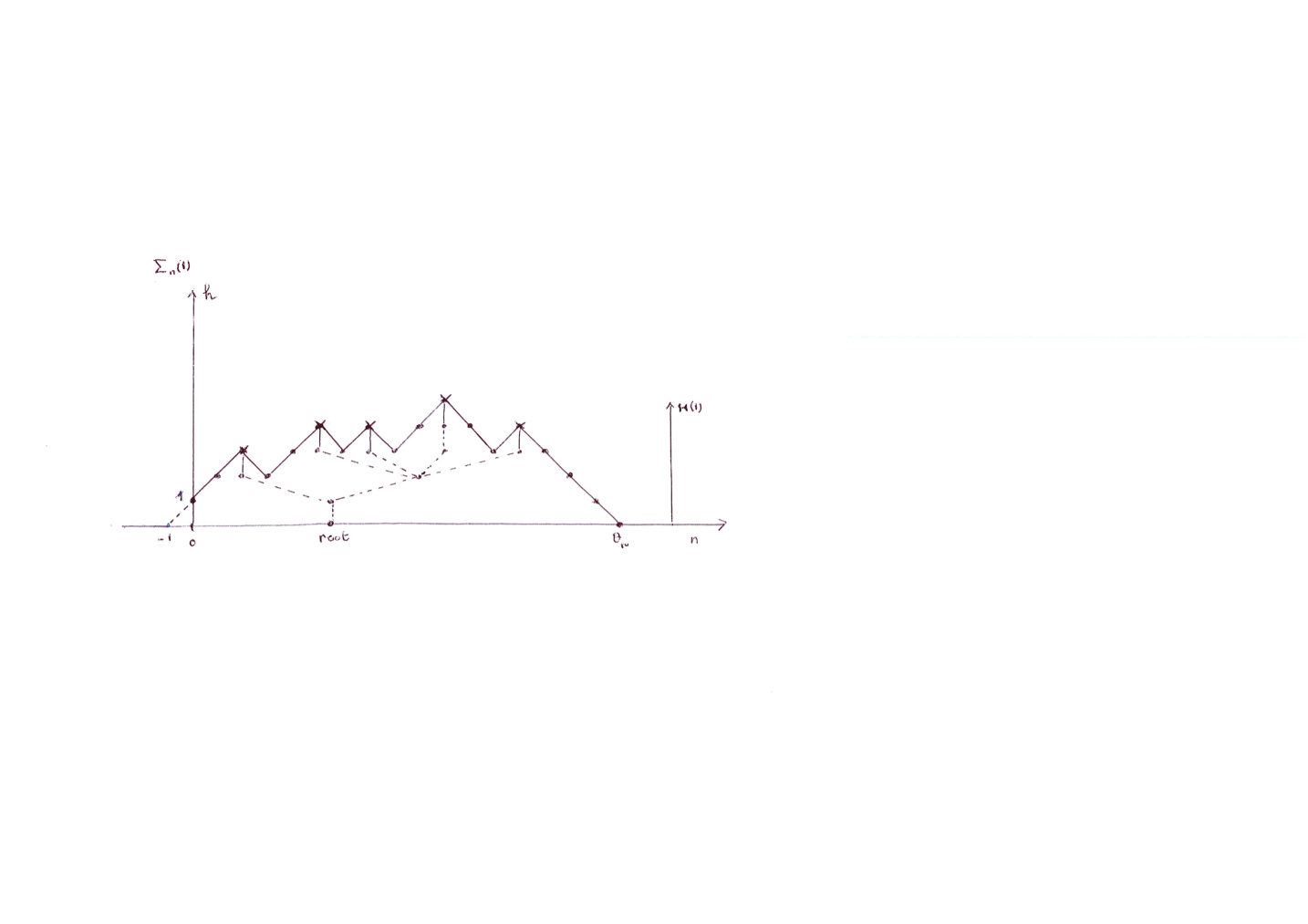
Figure 1. A realization of the SRW $\Sigma_{n}\left(1\right)$ and its nested BGW (dotted lines). On top of its leaves, additional fictitious branches were added to join the maxima of the SRW.

For instance, for the realization $0123234343454343210$ of a SRW excursion starting at $0$ at $n=-1$, $\mathcal{N}_{h}\left(1\right)=1,1,2,4,1$ for $h=0,...,4$, (see Figure $1$).

Following [Harris, 1952], $\mathcal{N}_{h}\left(1\right)$ is a BGW process with Geo${}_{0}\left(q_{0}\right)$ branching mechanism

$$\bullet\text{ }\mathcal{\phi}_{SRW}\left(z\right)=\text{ }q_{0}+\left(1-q_{0}\right)\frac{\left(1-p_{0}\right)z}{1-p_{0}z}=\frac{q_{0}}{1-p_{0}z}.$$

By first-step analysis indeed, for each $h\geq 1$ and given $m\geq 1$, the probability $P\left(m\right)$ of any path event: $+\cdot\cdot\cdot\left(m-1\right)+\cdot\cdot\cdot-$ coding the event that $m-1$ moves up occurred at height $h$ between events of a rise point $+$ ($h-1\rightarrow h$) and the subsequent (random) fall point $-$ ($h\rightarrow h-1$) (without the path visiting states below $h$ in between) obeys:

$$P\left(m\right)=\left\{\begin{array}[]{c}\delta_{m,0}\text{ w.p. }q_{0}\\ P\left(m-1\right)\text{ w.p. }p_{0}=1-q_{0}.\end{array}\right.$$

The p.g.f. of $P\left(m\right)$ is thus $\phi_{SRW}\left(z\right)=\sum_{m\geq 0}P\left(m\right)z^{m}$ obeying $\phi_{SRW}\left(z\right)=q_{0}+p_{0}z\phi_{SRW}\left(z\right).$ Each such sub-excursion $+\cdot\cdot\cdot\left(m-1\right)+\cdot\cdot\cdot-$ has the same law as the one of the original full excursion when we shift its levels by a vertical translation $-\left(h-1\right)$.

The range of $h$ is $\left\{0,...,\mathcal{H}\left(1\right)-1\right\}$ where $\mathcal{H}\left(1\right)$ is the height of any highest peak of the SRW or the BGW’s process lifetime shifted by one unit. An individual in the $(h-1)$-st generation has thus a probability $\left(1-q_{0}\right)p_{0}^{m-1}\left(1-p_{0}\right)=q_{0}p_{0}^{m}$ of having exactly $m$ children, $m=0,1,..$. (The ancestor being the $0$ generation).

Clearly, there exists a similar quantity of $\mathcal{N}_{h}\left(1\right)$ for the fall points $h\rightarrow h-1$ of the SRW for each $h\geq 1$. When summing both over $h\geq 0$, these numbers are equal (when the SRW is a $\left(0,0\right)-$ excursion) and the sum of the two is $1+\mathcal{\theta}_{1,0}$. Note that the local maxima of the walk are not taken into account in $\mathcal{N}_{h}\left(1\right)$.

The rise points of the SRW at $h$ are the offspring of the nodes of the BGW tree at $h-1$. Starting from the root at $h=0$, the tree grows without branching below the SRW’s profile, until it meets its first $m\geq 1$ local minima. The BGW process produces there $m+1$ offspring ($m$ of which corresponding to finite sub-excursions of the SRW) and starting from the right-most local first minimum, the process can be repeated along independent pieces of the SRW’s profile. The r.v. $\mathcal{N}_{h}\left(1\right)-1$ is thus the number of local minima of an excursion of the SRW at height $h$. For this BGW process, it is then easy to count the random number of out-degree-$d$ nodes, $d=\left\{0,1,...\right\}$, for each $h$, in particular the leaves ($d=0$) and the non-branching nodes ($d=1$). To complete the picture, on top of each leaf of the tree a fictitious additional branch (edge) can be added, ending up on the local maxima of the SRW (see Figure $1$). The height of a highest leaf of the nested BGW tree (its extinction time $\mathcal{\tau}_{1,0}$) corresponds to the one of a highest peak $\mathcal{H}\left(1\right)$ of the SRW, so with $\mathcal{H}\left(1\right)=\mathcal{\tau}_{1,0}+1$. Clearly, $\overline{\mathcal{N}}_{\mathcal{\tau}_{1,0}}\left(1\right):=\sum_{h=0}^{\mathcal{\tau}_{1,0}}\mathcal{N}_{h}\left(1\right)$ is the total number of individuals ever born in the course of this Galton-Watson process and, with

$$\mathcal{A}\left(1\right) = \sum_{n=0}^{\mathcal{\theta}_{1,0}-1}\Sigma_{n}\left(1\right)$$

$$\mathcal{B}\left(1\right) = \sum_{n=0}^{\mathcal{\theta}_{1,0}-1}\Sigma_{n}\left(1\right)-\sum_{n=0}^{\mathcal{\theta}_{1,0}-1}\left(\Sigma_{n}\left(1\right)-\Sigma_{n+1}\left(1\right)\right)_{+},$$

respectively the area and the restricted area under the (broken-line) profile of the SRW, taking into account only the areas of the configurations $\square$ but not the ones $\bigtriangleup$ or pairs of half such triangles:

$$\mathcal{B}\left(1\right)=2\sum_{h=1}^{\mathcal{\tau}_{1,0}}h\mathcal{N}_{h}\left(1\right).$$

For the realization $0123234343454343210$ of the SRW excursion, $\mathcal{A}\left(1\right)=51$, $\mathcal{B}\left(1\right)=42$ and $\sum_{h=1}^{\mathcal{\tau}_{1,0}}h\mathcal{N}_{h}\left(1\right)=21.$

Defining the p.g.f. $\emph{h}_{i}\left(z\right):=\mathbf{E}\left(z^{\mathcal{\theta}_{i,0}}\right)$, upon conditioning on the first step

$$\emph{h}_{1}\left(z\right)=q_{0}z+p_{0}z\emph{h}_{2}\left(z\right)$$

with $\emph{h}_{2}\left(z\right)=\emph{h}_{1}\left(z\right)^{2}.$ Thus,

$$\emph{h}\left(z\right)=\frac{1-\sqrt{1-4p_{0}q_{0}z^{2}}}{2p_{0}z},$$

and, with $k\geq 1,$

$$\mathbf{P}\left(\mathcal{\theta}_{1,0}=2k-1\right)=\frac{\left(p_{0}q_{0}\right)^{k}}{p_{0}}\frac{\binom{2k-2}{k-1}}{k!}.$$

In the critical case $p_{0}=q_{0}=1/2,$ $\mathcal{\theta}_{1,0}$ has Pareto tails with index $1/2$.

We have $\emph{h}\left(1\right)=\mathbf{P}\left(\mathcal{\theta}_{1,0}<\infty\right)=\frac{1-\left|p_{0}-q_{0}\right|}{2p_{0}}=1\wedge q_{0}/p_{0}$, translating that when $p_{0}>q_{0}$, the SRW is transient. At the same time, the nested BGW process is subcritical if $q_{0}/p_{0}>1$, critical if $q_{0}/p_{0}=1$ and supercritical if $q_{0}/p_{0}<1.$ In this last case, $\mathcal{\tau}_{1,0}=\inf\left(h\geq 1:\mathcal{N}_{h}\left(1\right)=0\right)<\infty$ only with positive probability $\rho_{e}=q_{0}/p_{0}$, the extinction probability of $\emph{N}_{h}\left(1\right)$, whereas in the first two cases, $\mathcal{\tau}_{1,0}<\infty$ a.s.. As required, we have: $\mathbf{P}\left(\mathcal{\theta}_{1,0}<\infty\right)=\mathbf{P}\left(\mathcal{\tau}_{1,0}<\infty\right).$

The p.g.f. $\Phi\left(z\right)$ of the total number of nodes of a BGW process with the geometric branching mechanism $\mathcal{\phi}_{SRW}\left(z\right)$ solves $\Phi\left(z\right)=z\mathcal{\phi}_{SRW}\left(\Phi\left(z\right)\right)$, leading to

$$\Phi\left(z\right) : =\mathbf{E}\left(z^{\overline{\mathcal{N}}_{\mathcal{\tau}_{1,0}}\left(1\right)}\right)=\frac{1-\sqrt{1-4p_{0}q_{0}z}}{2p_{0}}$$

$$\mathbf{P}\left(\overline{\mathcal{N}}_{\mathcal{\tau}_{1,0}}\left(1\right)=k\right) = \frac{\left(p_{0}q_{0}\right)^{k}}{p_{0}}\frac{\left(2k-2\right)!}{k!\left(k-1\right):},\text{ }k\geq 1.$$

Hence: $\Phi\left(z^{2}\right)=z\emph{h}\left(z\right),$ translating that $\mathcal{\theta}_{1,0}\overset{d}{=}2\overline{\mathcal{N}}_{\mathcal{\tau}_{1,0}}\left(1\right)-1.$

In the critical case when $p_{0}=q_{0}=1/2$, it can be checked that $\overline{\mathcal{N}}_{\mathcal{\tau}_{1,0}}\left(1\right)$ has Pareto tails with index $1/2$ just like $\mathcal{\theta}_{1,0}$ therefore.

Remark: the paths of the SRW excursion can be reconstructed from the one of its nested BGW tree as follows (see Figure 1):

Start from any prolific node of the nested tree at height $h\geq 0$ and consider the subtree rooted at this node. Browsing this subtree following the contour process strategy yields the sub-excursion of the SRW above level $h+1.$ If the starting node has outdegree $d\geq 1$, there are $d$ returns at level $h+1$ of the sub-excursion. In the processes, all the edges are visited twice. [see Champagnat (2015), pages $33$ and $38$, for example]. $\blacksquare$

Define now $\theta_{1,0}$ to be the time of the first visit to the origin of the $\left\{p,q,r\right\}-$SRW $\Sigma_{n}\left(1\right)$. We define

$$A\left(1\right)=\sum_{n=0}^{\theta_{1,0}-1}\Sigma_{n}\left(1\right);\text{ }H\left(1\right)=\underset{n=0,...,\theta_{1,0}-1}{\max}\Sigma_{n}\left(1\right),$$

respectively the area under the profile of $\Sigma_{n}\left(1\right)$ and its height. We also let, as before,

$$B\left(1\right)=\sum_{n=0}^{\theta_{1,0}-1}\Sigma_{n}\left(1\right)-\sum_{n=0}^{\theta_{1,0}-1}\left(\Sigma_{n}\left(1\right)-\Sigma_{n+1}\left(1\right)\right)_{+}$$

be the restricted area under the profile of $\Sigma_{n}\left(1\right)$.

For each $h\geq 1,$ with $G_{n,h}$ an i.i.d. sequence of Geo${}_{0}\left(r\right)-$distributed r.v.’s define the additive functional

$$\bullet\text{ }N_{h}\left(1\right)=\sum_{n=0}^{\theta_{1,0}-1}\left(G_{n,h}\mathbf{1}_{\left\{\Sigma_{n}\left(1\right)=h;\text{ }\Sigma_{n+1}\left(1\right)=h+1\right\}}\right),\text{ }N_{0}\left(1\right)=1.$$

In words, $N_{h}\left(1\right)$ is the number of times that, before first visiting $0,$ the random walk $\Sigma_{n}\left(1\right)$ crosses from $h$ to $h+1$ (the rise points of the SRW) to which the sizes of each $h+1$-plateau forming the left terraces were attached. The local highlands of the SRW are not taken into account in $N_{h}\left(1\right)$. For instance, for the realization $01(222)(33)23(4444)3434(55)4343210$ of a SRW excursion with plateaus starting at $0$ at $n=-1$, $N_{h}\left(1\right)=1,3,3,7,2$ for $h=0,...,4.$ Clearly there exists a similar symmetric quantity for the fall points $h\rightarrow h-1$ of the SRW for each $h\geq 1$, with plateaus now preceding the fall points (the right terraces). When summing both over $h\geq 0$, these numbers are equal in distribution (when the SRW is a $\left(0,0\right)-$ excursion) and the sum of the two is $1+\theta_{1,0}$ in law. If we define the width $\Sigma_{\theta_{1,0}}^{**}\left(1\right)$ of $\Sigma_{n}\left(1\right)$ as the largest size of the valleys in its profile, then

$$\Sigma_{\theta_{1,0}}^{**}\left(1\right)=\max_{h=1,...,\tau_{1,0}}N_{h}\left(1\right)=:N_{\tau_{1,0}}^{*}\left(1\right),$$

so the maximal value which the crossing process $N_{h}\left(1\right)$ can take.

The sequence $N_{h}\left(1\right)$ is a BGW process with LF offspring distribution (14), with the correspondence:

(56) $$\overline{\pi}=p,\text{ }\pi_{0}=q\text{ and }\pi-\pi_{0}=r>0,$$

so with the restriction $\pi>\pi_{0}$ ($r>0$). Equivalently, the branching mechanism of the BGW process nested inside the SRW is

(57a) $$\bullet\text{ }\phi_{SRW}\left(z\right)=q+\left(1-q\right)\frac{\left(1-p\right)z}{1-pz}=\frac{q+rz}{1-pz}.$$

Proof: An individual in the $\left(h-1\right)$st generation has a probability $\left(1-q\right)p^{m-1}\left(1-p\right)$ of having exactly $m$ children, $m=1,2,...$, given it is productive; its probability of having no offspring being $q$ (The ancestor being at generation $0$). This probability mass function enjoys the memory-less property of the geometric distribution.

By first-step analysis, for each $h\geq 1$ and given $m\geq 1$, the probability $P\left(m\right)$ of any path event $+\cdot\cdot\cdot\left(m-1\right)+\cdot\cdot\cdot-$ coding the event that $m-1$ moves up occurred at height $h$ between events of the type $+$ ($h-1\rightarrow h$) and the subsequent $-$ ($h\rightarrow h-1$) (without the path visiting states below $h$ in between and including no move steps between the extremities) obeys:

$$P\left(m\right)=\left\{\begin{array}[]{c}\delta_{m,0}\text{ w.p. }q\\ \delta_{m,1}\text{ w.p. }r\\ P\left(m-1\right)\text{ w.p. }p.\end{array}\right.$$

With probability $r$, the path configuration is $+0\cdot\cdot\cdot 0-$, the one of a highland at height $h$, so with $m=1$ (no move up in between the extremities). The p.g.f. of $P\left(m\right)$ is $\phi_{SRW}\left(z\right)=\sum_{m\geq 0}P\left(m\right)z^{m}$ obeying $\phi_{SRW}\left(z\right)=q+rz+pz\phi_{SRW}\left(z\right).$ We call the linear-fractional BGW process with branching mechanism $\phi_{SRW}\left(z\right)$ the nested BGW process inside the $\left\{p,q,r\right\}-$SRW.

Note that the nested BGW process is subcritical if $\pi_{0}/\overline{\pi}=q/p>1$, critical if $\pi_{0}/\overline{\pi}=q/p=1$ and supercritical if $\pi_{0}/\overline{\pi}=q/p<1.$ In this last case, $\tau_{1,0}=\inf\left(h\geq 1:N_{h}\left(1\right)=0\right)<\infty$ only with positive probability $\rho_{e}=q/p$, the extinction probability of $N_{h}\left(1\right)$, whereas in the first two cases, $\theta_{1,0}<\infty$ a.s.. Concomitantly, $\mathbf{P}\left(\theta_{1,0}<\infty\right)=\frac{1-\left|p-q\right|}{2p}=1\wedge q/p$, translating that when $p>q$, the SRW is transient at infinity. As required, in all cases, we have: $\mathbf{P}\left(\theta_{1,0}<\infty\right)=\mathbf{P}\left(\tau_{1,0}<\infty\right).$

As before, we let $\overline{N}_{\tau_{1,0}}\left(1\right)=\sum_{h=0}^{\tau_{1,0}}N_{h}\left(1\right)$ the total number of nodes of the BGW tree with branching mechanism (57a).

$\bullet$ By first-step analysis, we have the correspondences:

$$H\left(1\right)\overset{d}{=}\tau_{1,0}+1$$

$$\theta_{1,0}\overset{d}{=}2\overline{N}_{\tau_{1,0}}\left(1\right)-1$$

$$\Sigma_{\theta_{1,0}}^{**}\left(1\right)\overset{d}{=}N_{\tau_{1,0}}^{*}\left(1\right)$$

$$B\left(1\right)\overset{d}{=}2\sum_{h=1}^{H\left(1\right)-1}hN_{h}\left(1\right)$$

Proof: We already mentioned the first one. We prove the second one, the other ones being obtained similarly.

Defining the p.g.f. $h_{i}\left(z\right):=\mathbf{E}\left(z^{\theta_{i,0}}\right)$, upon conditioning on the first step

$$h_{1}\left(z\right)=qz+rzh_{1}\left(z\right)+pzh_{2}\left(z\right)$$

with $h_{2}\left(z\right)=h_{1}\left(z\right)^{2}.$ Thus

$$h\left(z\right):=h_{1}\left(z\right)=\mathbf{E}\left(z^{\theta_{1,0}}\right)=\frac{1-rz-\sqrt{\left(1-rz\right)^{2}-4pqz^{2}}}{2pz}$$

with, as required while considering that the lengths of the plateaus are Geo${}_{0}\left(r\right)-$distributed,

$$h\left(z\right)=\frac{1-\sqrt{1-4p_{0}q_{0}z^{2}}}{2p_{0}z}\mid_{z\rightarrow\frac{\left(1-r\right)z}{1-rz}}$$

Now the p.g.f. $\Phi\left(z\right)=\mathbf{E}\left(z^{\overline{N}_{\tau_{1,0}}\left(1\right)}\right)$ of the total number of nodes of a BGW process with general LF branching mechanism $\phi\left(z\right)$ solves $\Phi\left(z\right)=z\phi\left(\Phi\left(z\right)\right)$, leading to

$$\Phi\left(z\right)=\frac{1-\left(\pi-\pi_{0}\right)z-\sqrt{\left(1-\left(\pi-\pi_{0}\right)z\right)^{2}-4\pi_{0}\overline{\pi}z}}{2\overline{\pi}}.$$

When dealing with $\phi_{SRW}\left(z\right)$ with the correspondences (56), $\Phi\left(z\right)$ becomes $\Phi_{SRW}\left(z\right)$ obeying:

$$\Phi_{SRW}\left(z^{2}\right)=zh\left(z\right),$$

translating that $\theta_{1,0}\overset{d}{=}2\overline{N}_{\tau_{1,0}}\left(1\right)-1.$ When $p=q$, $\theta_{1,0}$ has Pareto tails with index $1/2$. This extends Theorem $5$ of [Harris, 1952].

- The height $H\left(1\right)\geq 1$ of the highest maximum or peak of $\Sigma_{n}\left(1\right)$ (as attained by the random walk before its first return to the origin) can be identified to $\tau_{1,0}+1$ where $\tau_{1,0}$ is the extinction time of the LF BGW tree associated to the SRW. Its distribution is thus given recursively by

$$\mathbf{P}\left(H\left(1\right)\leq h+1\right)=\phi_{SRW}\left(\mathbf{P}\left(H\left(1\right)\leq h\right)\right),\text{ }h\geq 0.$$

We get

$$\mathbf{P}\left(H\left(1\right)>h\right) = \frac{1}{\left(\frac{1-p}{1-q}\right)^{h}+\frac{p}{1-q}\left(1+...+\left(\frac{1-p}{1-q}\right)^{h-1}\right)}$$

$$= \frac{p-q}{p-q\left(\frac{1-p}{1-q}\right)^{h}}\text{ if }p\neq q$$

$$= \frac{1-p}{1+p\left(h-1\right)}\text{ if }p=q.$$

When $p=q$, $H\left(1\right)$ has Pareto tails with index $1$.

- The height $L\left(1\right)$ of the lowest minimum of $\Sigma_{n}\left(1\right)$ (else, the height of the deepest valley of the SRW’s profile) is the first time at which a fictitious leaf appears in $\left\{N_{h}\left(1\right)\right\}$. Its distribution is Geo$\left(\pi_{1}\right),$ with $\pi_{1}=\phi_{SRW}^{{}^{\prime}}\left(0\right)=\left(1-p\right)\left(1-q\right),$the probability that the associated BGW process generates a single offspring, so

$$\mathbf{P}\left(L\left(1\right)=h\right)=\overline{\pi}_{1}\pi_{1}^{h-1},\text{ }h\geq 1.$$

- From (51),

(58) $$\mathbf{P}\left(\overline{N}_{\tau_{1,0}}\left(1\right)=n\right)=q^{n}\left(a*b\right)_{n-1}\text{ with}$$

$$a_{k}=\binom{n}{k}\left[r/q\right]^{k}\text{ and }b_{k}=\binom{n+k-1}{n-1}p^{k}.$$

In the critical case when $p=q$, $\overline{N}_{\mathcal{\tau}_{1,0}}\left(1\right)$ has Pareto tails with index $1/2$ and so does $\theta_{1,0}$ therefore.

- The law of $N_{\tau_{1,0}}^{*}\left(1\right)$ and also of $\Sigma_{\theta_{1,0}}^{**}\left(1\right)$ is given by $\mathbf{P}\left(N_{\tau_{1,0}}^{*}\left(1\right)\leq 1+j\right)=\frac{w\left(j\right)}{w\left(1+j\right)}$, with $w\left(j\right)$ the scale function defined in (55).

The SRW $\Sigma_{n}\left(1\right)$ looks very much like the profile of a mountain chain. By considering the reflected SRW $-\Sigma_{n}\left(1\right)$, the physical image is the one of a seabed profile. The highlands of $\Sigma_{n}\left(1\right)$ become the valleys of $-\Sigma_{n}\left(1\right).$

While considering the concatenation of $i\geq 2$ i.i.d. excursion landscapes of the SRW (assuming state $0$ to be purely reflecting), the BGW to consider is $N_{h}\left(i\right),$ being $i$ i.i.d. copies of $N_{h}\left(1\right).$

[Harris (1952)] observes that the connection of BGW processes and simple SRWs remains valid if the transition probabilities $\left(p_{h},q_{h}\right),$ $p_{h}+q_{h}=1,$ of the (non-homogeneous) SRW depend on its current height $h$; the nested BGW process has then a corresponding branching mechanism depending on the height: $\mathbf{P}\left(M_{h}=m\right)=\left(1-q_{h+1}\right)p_{h+1}^{m-1}\left(1-p_{h+1}\right)=q_{h+1}p_{h+1}^{m}$ ($p_{h+1}+q_{h+1}=1$), $h\geq 0,$ $m\geq 1$. The iteration of variable height-dependent LF branching mechanisms is then necessary.

Acknowledgments:

T. Huillet acknowledges partial support from the “Chaire Modélisation mathématique et biodiversité” of Veolia-Ecole Polytechnique-MNHN-FondationX and support from the labex MME-DII Center of Excellence (Modèles mathématiques et économiques de la dynamique, de l’incertitude et des interactions, ANR-11-LABX-0023-01 project). This work was also funded by CY Initiative of Excellence (grant “Investissements d’Avenir”ANR- 16-IDEX-0008), Project “EcoDep” PSI-AAP2020-0000000013. S. Martínez was supported by the Center for Mathematical Modeling ANID Basal FB210005.

Declarations of interest

The authors have no conflicts of interest associated with this paper.

Data availability statement

There are no data associated with this paper.

References

- [1] Athreya, K. B. & Ney, P. (1972). Branching Processes. Springer, New York.
- [2] Avan, J., Grosjean, N. & Huillet, T. (2015). Did the ever dead outnumber the living and when? A birth-and-death approach. Physica A: Statistical Mechanics and its Applications, Volume 419, 277-292.
- [3] Avram, F. & Vidmar, M. (2019). First passage problems for upwards skip-free random walks via the scale functions paradigm. Advances in Applied Probability, 51(2), 408-424.
- [4] Bennies, J. & Kersting, G. (2000). A Random Walk Approach to Galton Watson Trees. Journal of Theoretical Probability, Vol. 13, No. 3, 777-803.
- [5] Bertoin J. (2000). Subordinators, Lévy processes with no negative jumps and branching processes. Lecture Notes of the Concentrated Advanced Course on Lévy Processes, Maphysto, Centre for Mathematical Physics and Stochastics, Department of Mathematical Sciences, University of Aarhus.
- [6] Brown, M., Peköz, E. A. & Ross, S. M. (2010). Some results for skip-free random walk. Probability in the Engineering and Informational Sciences, 24(4), 491-507.
- [7] Champagnat, N. (2015) Processus de Galton-Watson et applications en dynamique des populations. Master. École Supérieure des Sciences et Technologies de Hammam Sousse, Tunisie. 2015, pp.46. ffcel-01216832ff
- [8] Comtet, L. (1970). Analyse Combinatoire. Tomes 1 et 2. Presses Universitaires de France, Paris.
- [9] Corral, Á, Garcia-Millan, R. & Font-Clos, F. (2016). Exact Derivation of a Finite-Size Scaling Law and Corrections to Scaling in the Geometric Galton-Watson Process. PLoS One. 11(9).
- [10] Cramér, H. (1938). Sur un nouveau théorème-limite de la théorie des probabilités. Actualités Scientifiques et Industrielles, 736, 523.
- [11] Drmota, M. (2009). Random Trees: An Interplay between Combinatorics and Probability. (1st ed.). Springer Publishing Company, Incorporated.
- [12] Dwass, M. (1969). The total progeny in a branching process and a related random walk. Journal of Applied Probability,Vol. 6, No. 3, pp. 682-686.
- [13] Flajolet, P. & Sedgewick, R. (1993). The average case analysis of algorithms: complex asymptotics and generating functions. [Research Report] RR-2026, INRIA inria-00074645.
- [14] Garcia-Millan R., Font-Clos F., Corral Á. (2015). Finite-size scaling of survival probability in branching processes. Phys Rev E., 91(4).
- [15] Good, I. J. (1949). The number of individuals in a cascade process. Proceedings of the Cambridge Philosophical Society, 45, 360-363.
- [16] Grosjean, N. & Huillet, T. (2017). Additional aspects of the generalized linear-fractional branching process. Annals of the Institute of Statistical Mathematics, vol. 69, issue 5, No 7, 1075-1097.
- [17] Harris, T. E. (1952). First passage and recurrence distributions. Transactions of the American Mathematical Society, Vol. 73, No. 3, pp. 471-486.
- [18] Harris, T. E. (1963). The theory of branching processes. Die Grundlehren der Mathematischen Wissenschaften, Bd. 119 Springer-Verlag, Berlin; Prentice-Hall, Inc., Englewood Cliffs, N.J.
- [19] Hoppe, F. M. (1980). On a Schröder equation arising in branching processes. Aequationes Mathematicae, 20(1), 33-37.
- [20] Howard J. (2012). World Population Explained: Do Dead People Outnumber Living, Or Vice Versa? Huffington Post, available at http://www.huffingtonpost.com/2012/11/07/world-populationexplained n 2058511.html.
- [21] Jagers, P. (2020) Branching Processes: A Personal Historical Perspective. Chapter 18 in: A. Almudevar et al. (Eds.) Statistical Modeling for Biological Systems. Springer International.
- [22] Kendall, D. G. (1966). Branching Processes Since 1873. Journal of the London Mathematical Society. Volumes1-41, Issue 1, 385-406.
- [23] Kingman, J. F. C. (1965). Stationary Measures for Branching Processes. Proceedings of the American Mathematical Society, Vol. 16, No. 2, pp. 245-247.
- [24] Klebaner, F. C., Rösler, U. & Sagitov, S. (2007). Transformations of Galton-Watson processes and linear fractional reproduction. Advances in Applied Probability, Volume 39, Number 4, 1036-1053.
- [25] Lambert, A. (2010). Some aspects of discrete branching processes. http://www.cmi.univ-mrs.fr/~pardoux/Ecole_CIMPA/CoursALambert.pdf.
- [26] Lamperti J. W. (1967). Continuous state branching processes. Bulletin of the American Mathematical Society, 73, 382-386.
- [27] Lamperti, J. W. & Ney, P. (1968). Conditioned branching processes and their limiting diffusions. Theory of Probability and its Applications, 13, 128-139.
- [28] Lindvall, T. (1976). On the Maximum of a Branching Process. Scandinavian Journal of Statistics, Vol. 3, No. 4, pp. 209-214.
- [29] Marchal, P. (2001). A combinatorial approach to the two-sided exit problem for left-continuous random walks. Combinatorics, Probability and Computing, 10(03), 251-266.
- [30] Otter, R. (1949). The multiplicative process. The Annals of Mathematical Statistics, 20, 206-224.
- [31] Norris, J. R. (1998). Markov chains. Cambridge University Press.
- [32] A. G. Pakes, A.G. (1971). Some limit theorems for the total progeny of a branching process. Advances in Applied Probability, Vol. 3, No. 1, pp. 176-192.
- [33] Pitman, J. (2006). Combinatorial stochastic processes. Lectures from the nd Summer School on Probability Theory held in Saint-Flour, July 7-24, 2002. With a foreword by Jean Picard. Lecture Notes in Mathematics, 1875. Springer-Verlag, Berlin.
- [34] Rényi, A. (1959). Some remarks on the theory of trees. MTA Mat. Kut. Int. Kozl, 4, 73-85.
- [35] Rogers, L. C. G. & Williams, D. (1994). Diffusions, Markov processes and Martingales. Vol 1, Foundations, 2nd edition, John Wiley, Chichester.
- [36] Sagitov, S. & Lindo, A. (2015). A special family of Galton-Watson processes with explosions. In Branching Processes and Their Applications. Lecture Notes in Statistics - Proceedings. (I.M. del Puerto et al eds.) Springer, Berlin, 2016 (to appear). arxiv.org/pdf/1502.07538.
- [37] Schröder, E. (1871). Über iterierte funktionen. Mathematische Annalen, 3, 296-322.
- [38] Sheth, R. (1996). Galton-Watson branching processes and the growth of gravitational clustering. Monthly Notices of the Royal Astronomical Society, Volume 281, Issue 4, 1277-1289.
- [39] Sibuya, M. (1979). Generalized hypergeometric, digamma and trigamma distributions. Annals of the Institute of Statistical Mathematics, 31, 373-390.
- [40] Steffenson, J. F. (1930). “On Sandsynligheden for at Afkommet uddor”, Matem. Tiddskr. B, 19-23.
- [41] Steffenson. J. F. (1933). Deux problèmes du calcul des probabilités. Annales de l’ Institut Henri Poincaré, 3, 319-344.
- [42] Takács, L. (1967). On combinatorial methods in the theory of stochastic processes. Proceedings of the Fifth Berkeley Symposium on Mathematical Statistics and Probability, Volume 2: Contributions to Probability Theory, Part 1, Vol. 5.2A.
- [43] Woess, W. (2009). Denumerable Markov chains. Generating functions, boundary theory, random walks on trees. EMS Textbooks in Mathematics. European Mathematical Society (EMS), Zürich.
- [44] Yaglom, A. M. (1947). Certain limit theorems of the theory of branching stochastic processes. Doklady Akademii Nauk SSSR, 56, 795-798.