Reimagining Demand-Side Management with Mean Field Learning

Abstract

Integrating renewable energy into the power grid while balancing supply and demand is a complex issue, given its intermittent nature. Demand side management (DSM) offers solutions to this challenge. We propose a new method for DSM, in particular the problem of controlling a large population of electrical devices to follow a desired consumption signal. We model it as a finite horizon Markovian mean field control problem. We develop a new algorithm, MD-MFC, which provides theoretical guarantees for convex and Lipschitz objective functions. What distinguishes MD-MFC from the existing load control literature is its effectiveness in directly solving the target tracking problem without resorting to regularization techniques on the main problem. A non-standard Bregman divergence on a mirror descent scheme allows dynamic programming to be used to obtain simple closed-form solutions. In addition, we show that general mean-field game algorithms can be applied to this problem, which expands the possibilities for addressing load control problems. We illustrate our claims with experiments on a realistic data set.

1 Introduction

Climate change is a complex problem, for which action takes many forms. Of the top 20 solutions identified by Foley et al. [2020] to reverse global warming, six are related to the energy sector, including integrating renewables into the electricity system and increasing the number of electric vehicles as a primary mode of transportation. In addition, the study managed by RTE [2022] showed that achieving carbon neutrality by 2050 in the French electricity scenario requires a decrease in final energy consumption and strong growth in renewable energy.

However, it is extremely difficult to make these solutions economically viable while also scaling them up. The intermittent nature of renewable energy sources can cause significant fluctuations in energy demand and supply, which may impact the balance of the power grid. Current solutions to keep the system in balance rely heavily on fossil fuel power plants, which have significant environmental costs, or on energy imports, which have capital and operating costs. Demand Side Management (DSM) are strategies to reduce energy acquisition costs and associated penalties by continuously monitoring energy consumption and managing devices [Bakare et al., 2023], which provides flexibility and improves the reliability of energy systems. Yet, implementing DSM solutions is challenging, as it involves large-scale data processing and near real-time scenarios. For this reason, machine learning solutions have recently emerged to solve DSM problems [Antonopoulos et al., 2020] with examples ranging from using multi-armed bandits to develop pricing solutions [Brégère et al., 2019], to deep learning models for smart charging of electric vehicles [López et al., 2019].

The goal of this paper is to make a new contribution to this field by proposing a new solution to a DSM problem concerning the control of thermostatically controled loads (TCLs: flexible appliances such as water heaters, air conditioners, refrigerators, etc). The aim is to control the aggregate power consumption of a large population of water heaters in order to follow a target consumption profile. To this end, we consider a finite time horizon Markovian mean field control (MFC) problem, and we propose a new algorithm based on mirror descent. We also adapt other mean field learning algorithms from the literature for this purpose.

Contributions

In this paper, we propose and compare two new approaches to solve a DSM problem: a new algorithm, MD-MFC, for general Markovian MFC problems, and an adaptation of existing algorithms in the mean field learning literature for game problems. First we provide a modeling of the management system in question as a Markov decision process (MDP) in Section 2. The literature review of previous modeling and solutions to the load control problem, as well as a discussion of the main ingredient of our algorithms, mean field learning, are postponed to Subection 2.3. Our main results are stated in Section 3: we introduce the MD-MFC algorithm for a Markovian MFC problem, and we prove a convergence rate of order $\smash{1/\sqrt{K}}$, where $K$ is the number of iterations, by linking it to a mirror descent [Nemirovski and Yudin, 1983] scheme. This implies a non-trivial reformulation of a non-convex problem in a measure space into a convex problem. A good choice of non-standard regularization allows dynamic programming [Bertsekas, 2005]. This results in the first algorithm that efficiently and directly solves the target tracking problem without resorting to regularization techniques in the main problem. Section 4 illustrates the results with simulations based on a realistic data set [Albouys et al., 2019]. A series of future works concludes the paper.

2 Setting and model

Our framework consists in modeling the random dynamics of a population of water heaters in order to control their average consumption to follow a target signal. From now on, for a finite set $S$, we define $\Delta_{S}$ to be the simplex of dimension $|S|$, the cardinal of $S$.

2.1 Randomized controlled dynamics for one water heater

Let us consider a discretisation of the time for $n=1,...,N$. At each time step $n$, the state of a water heater is described by a variable $x_{n}=(m_{n},\theta_{n})\in\mathcal{X}:=\{0,1\}\times\Theta$, where $m_{n}$ indicates the operating state of the heater (ON if $1$, OFF if $0$), and $\theta_{n}$ represents the average temperature of the water in the tank. For the sake of simplification we consider only temperatures inside a finite set $\Theta$.

We call the uncontrolled dynamics the nominal dynamics. A water heater that follows the nominal dynamics [Bušić and Meyn, 2016] obeys a cyclic ON/OFF decision rule with a deadband to ensure that the temperature is between a lower limit $T_{\text{min}}$ and an upper limit $T_{\text{max}}$. Thus, if the water heater is turned on, it heats water with the maximum power until its temperature exceeds $T_{\text{max}}$. Then, the heater turns off and the water temperature decreases until it reaches $T_{\text{min}}$, where the heater turns on again and a new cycle begins. The nominal dynamics at a discretized time is illustrated in Figure 1. The temperature at each time step is calculated by approximating an ordinary differential equation (ODE) depending on the current operating state of the heater and the hot water drawn at each time step (see Appendix D.1). We assume that the event of a water withdrawn is random and independent at each time step with a known probability distribution.

Figure 1: Temperature evolution of a water heater following the nominal dynamics.

In order to have a controllable model, we fit the nominal dynamics of a water heater to a Markov decision process. The finite state space is given by $\mathcal{X}$, and we consider an action space given by $\mathcal{A}:=\{0,1\}$. At time step $n$, choosing action $1$ means turning the heater on except when $\theta_{n}\geq T_{\text{max}}$. Conversely, choosing action $0$ means turning the heater off except when $\theta_{n}\leq T_{\text{min}}$. The nominal dynamics deterministically chooses action $0$ if the heater is off and $1$ if it is on, independent of the heater’s temperature. Unlike the nominal dynamics, we want to consider stochastic strategies for choosing actions. If the heater is in state $x_{n}=(m_{n},\theta_{n})$, the next temperature is computed by $\theta_{n+1}:=T(m_{n},\theta_{n},\epsilon_{n})$ where $T$ is a function defined as the solution of Equation (16) of Appendix D.1 and $\epsilon_{n}$ is the random variable corresponding to a water-withdraw event at time step $n$. The action $a_{n}$ is sampled with probability $\pi_{n}(\cdot|x_{n})\in\Delta_{\mathcal{A}}$, and the next operating state is given by $m_{n+1}:=M(a_{n},\theta_{n+1})$, where

$$M(a_{n},\theta_{n+1}):=a_{n}\mathds{1}_{\theta_{n+1}\in[T_{\text{min}},T_{\text{max}}]}+\mathds{1}_{\theta_{n+1}<T_{\text{min}}}.$$

Hence, the probability kernel for each time step $n$ is given by

$${p_{n+1}(x_{n+1}|x_{n},a_{n}):=\mathbb{P}\big{(}\theta_{n+1}=T(m_{n},\theta_{n},\epsilon_{n})|\theta_{n},m_{n}\big{)}\mathbb{P}\big{(}m_{n+1}=M(a_{n},\theta_{n+1})|a_{n},\theta_{n+1}\big{)}}.$$

Moreover if $\theta_{n+1}\in[T_{\text{min}},T_{\text{max}}]$, the action $a_{n}\sim\pi_{n}(\cdot|x_{n})$ defines the next operating state of the heater. For more details on our modeling of the dynamics of a water heater, see Appendix D.1.

2.2 Optimisation problem

Consider a population of $M$ water heaters indexed by $i$ and described at time step $n$ by $X_{n}^{i}=(m_{n}^{i},\theta_{n}^{i})$ following the randomized dynamics described in Subsection 2.1. We suppose all water heaters to be homogeneous, i.e. they have the same dynamics, and follow the same policy $\pi$. Let $\smash{\bar{m}_{n}:=\frac{1}{M}\sum_{i=1}^{M}m_{n}^{i}}$ denote the average consumption. We assume for simplicity that the maximum power of each water heater is $p_{\text{max}}=1$ so that the average consumption is equal to the proportion of heaters at state ON. Note that $\bar{m}_{n}$ depends on the policy $\pi$ that the water heaters follow, thus we can denote it as $\bar{m}_{n}(\pi)$. Let ${\gamma=(\gamma_{n})_{1\leq n\leq N}\in[0,1]^{N}}$ be our target consumption profile (for example, the energy production at each time step divided by the number of devices). Our goal is to solve the problem

$$\min_{\pi\in(\Delta_{\mathcal{A}})^{\mathcal{X}\times N}}\mathbb{E}\left[\sum_{n=1}^{N}(\bar{m}_{n}(\pi)-\gamma_{n})^{2}\right],$$ (1)

where we have chosen to work with a quadratic loss.

Let $\mu:=(\mu_{n})_{n\in[0,...,N]}$ such that $\mu_{n}$ is the state-action distribution of the entire population of heaters at time $n$. We denote by $\mu^{\pi}$ a state-action distribution sequence induced by a policy sequence $\pi$ such as in Definition 2.1.

Definition 2.1 (Distribution induced by a policy $\pi$).

Given an initial distribution $\mu_{0}$ fixed, the state-action distributions sequence induced by the policy sequence $\pi=(\pi_{n})_{1\leq n\leq N}$ is denoted $\mu^{\pi}:=(\mu^{\pi}_{n})_{1\leq n\leq N}$ and is defined recursively by

$$\begin{split}&\mu_{0}^{\pi}(x^{\prime},a^{\prime}):=\mu_{0}(x^{\prime},a^{\prime})\\ &\mu_{n+1}^{\pi}(x^{\prime},a^{\prime}):=\sum_{x\in\mathcal{X}}\sum_{a\in\mathcal{A}}\mu_{n}^{\pi}(x,a)p_{n+1}(x^{\prime}|x,a)\pi_{n+1}(a^{\prime}|x^{\prime}).\end{split}$$

For a function $\varphi:\mathcal{X}\rightarrow\mathbb{R}$, we define ${\mu_{n}(\varphi):=\sum_{x}\varphi(x)\mu_{n}(x,a)}$ for all $1\leq n\leq N$. We are particularly interested in a function $\varphi$ such that $\mu_{n}(\varphi)$ gives us the average consumption of our water heater’s population. Thus, we consider from now on

$$\begin{split}\varphi:\quad\mathcal{X}&\rightarrow\mathbb{R}\\ (m,\theta)&\mapsto m.\end{split}$$ (2)

For such a function $\varphi$, when $M\to\infty$, the mean field approximation [Jabin and Wang, 2017] of Problem (1) consists in the main mean field control problem considered in the paper, and is given by

$$\min_{\pi}F(\mu^{\pi}):=\sum_{n=1}^{N}f_{n}(\mu^{\pi}_{n}),$$ (3)

where ${f_{n}(\mu_{n}^{\pi}):=(\mu_{n}^{\pi}(\varphi)-\gamma_{n})^{2}}$.

It is important to mention that the algorithms and results presented in Section 3 for solving Problem (3) remain valid for any general finite horizon Markovian MFC problem with finite state and action spaces, where the cost functions $f_{n}$ are convex and Lipschitz with respect to the $\|\cdot\|_{1}$ norm.

2.3 Literature discussion

Decision-making problems formulated as such mean-field models are a popular framework for stochastic optimization problems in many applications, ranging from robotics Shiri et al. [2019], Elamvazhuthi and Berman [2019] to finance Achdou et al. [2014], Casgrain and Jaimungal [2018], energy management De Paola et al. [2019], Bušić and Meyn [2019], epidemic modeling Lee et al. [2021], and more recently, machine learning E et al. [2018], Ruthotto et al. [2020], Fouque and Zhang [2020], Lin et al. [2021]. Thus, although this paper focuses on a demand management problem, our results also provide a new approach to solving problems in many other areas.

Load control

Controlling the sum of the consumption of a large number of TCLs started being investigated around $1980$ by Ihara and Schweppe [1981], Malhame and Chong [1985], Mortensen and Haggerty [1988] establishing the first physically based modeling for a TCL population. In the works of Kizilkale and Malhame [2013, 2014], the difficulty due to the large number of devices is circumvented by a mean field approximation.

For water heater control, Cammardella et al. [2019] use a quadratic objective and a Kullback-Leibler (KL) penalty allowing a Lagrangian approach that learns both the control and the probability transition kernel, but cannot handle uncontrolled state parts, so uncertainties like water withdrawals must be modeled as deterministic. More recently, Cammardella et al. [2021] takes into account the uncontrolled stochastic environment in the KL quadratic control framework by adding constraints on the probability transition kernel. It is the KL penalty on the main problem that allows them to obtain their main results. However, there is a trade-off between adding the KL and obtaining a good target tracking curve. We therefore propose to solve directly the same quadratic control framework but without the KL penalty. We have successfully provided the first algorithm for direclty solving the target tracking problem.

Mean field learning

Mean field games (MFG) have been introduced by Lasry and Lions [2007] and Huang et al. [2006] to tackle the issue of games with a large number of symmetric and anonymous players, by passing to the limit of an infinite number of players interacting through the population distribution. Although MFG focuses on finding Nash equilibria (NE), social optima on cooperative setting have also been studied under the term of mean field control (MFC) [Bensoussan et al., 2013].

Lately, iterative learning methods such as fictitious play and online mirror descent have been adapted to the MFG scenario in Perrin et al. [2020] and Pérolat et al. [2022]. Geist et al. [2022] show an equivalence between Frank Wolfe’s classical optimization algorithm [Frank and Wolfe, 1956] and the fictitious play for potential structured games. Similarly, we show an equivalence between our MFC problem and potential games, that open up a new range of solutions to the DSM problem considered using the above studies.

3 Main results: algorithmic approaches

3.1 Building a new algorithm

Consider the set of state-action distributions sequences initialized at $\mu_{0}\in\Delta_{\mathcal{X}\times\mathcal{A}}$ and satisfying a specific constrained evolution given by

$$\begin{split}\mathcal{M}_{\mu_{0}}:=\bigg{\{}\mu\in(\Delta_{\mathcal{X}\times\mathcal{A}})^{N}\big{|}\;&\sum_{a^{\prime}\in\mathcal{A}}\mu_{n+1}(x^{\prime},a^{\prime})\\ &=\sum_{x\in\mathcal{X},a\in\mathcal{A}}p_{n+1}(x^{\prime}|x,a)\mu_{n}(x,a)\;,\forall x^{\prime}\in\mathcal{X},\forall n\in[0,...,N]\bigg{\}}.\end{split}$$ (4)

The set $\smash{\mathcal{M}_{\mu_{0}}}$ describes the sequences of state-action distribution respecting the dynamics of the Markov model. Furthermore, this set is convex [Cammardella et al., 2021].

Proposition 3.1.

Let $\mu_{0}\in\Delta_{\mathcal{X}\times\mathcal{A}}$. The application ${\pi\mapsto\mu^{\pi}}$ is a surjection from $(\Delta_{\mathcal{A}})^{\mathcal{X}\times N}$ to $\mathcal{M}_{\mu_{0}}$.

The idea of the proof of Proposition 3.1, reported to Appendix A, is that one can retrieve the policy sequence $\pi$ inducing the state-action distribution sequence $\mu$ by taking $\smash{\pi_{n}(a|x)=\frac{\mu_{n}(x,a)}{\rho_{n}(x)}}$, where $\smash{\rho_{n}(x):=\sum_{a\in\mathcal{A}}\mu_{n}(x,a)}$. Let $\smash{\mathcal{M}_{\mu_{0}}^{*}}$ denotes the subset of $\smash{\mathcal{M}_{\mu_{0}}}$ where the corresponding policies $\pi$ are such that $\pi_{n}(a|x)\neq 0$ for all $(x,a)\in\mathcal{X}\times\mathcal{A}$ and $1\leq n\leq N$. We define the regularization function $\smash{\Gamma:\mathcal{M}_{\mu_{0}}\times\mathcal{M}_{\mu_{0}}^{*}\to\mathbb{R}}$ as

$$\Gamma(\mu^{\pi},\mu^{\pi^{\prime}}):=\sum_{n=1}^{N}\mathbb{E}_{(x,a)\sim\mu{{}^{\pi}}_{n}(\cdot)}\bigg{[}\log\bigg{(}\frac{\pi_{n}(a|x)}{\pi^{\prime}_{n}(a|x)}\bigg{)}\bigg{]}.$$ (5)

Before giving a solution to Problem (3), we consider the following auxiliary optimization problem, which will later help us build the new algorithm. This iterative scheme is possible thanks to Proposition 3.1 which guarantees the existence of a strategy $\pi$ for any $\smash{\mu\in\mathcal{M}_{\mu_{0}}}$. Here, $k$ represents an iteration:

$$\begin{split}\mu^{k+1}\in\operatorname*{arg\,min}_{\mu^{\pi}\in\mathcal{M}_{\mu_{0}}}\bigg{\{}\langle\nabla F(\mu^{k}),\mu^{\pi}\rangle+\frac{1}{\tau_{k}}\Gamma(\mu^{\pi},\mu^{k})\bigg{\}}.\end{split}$$ (6)

We consider $\tau_{k}>0$ and $\smash{\langle\nabla F(\mu^{k}),\mu^{\pi}\rangle:=\sum_{n=1}^{N}\langle\nabla f_{n}(\mu_{n}^{k}),\mu_{n}^{\pi}\rangle}$. At iteration $k+1$, we want to find $\mu^{\pi}$ by minimizing a linearization of $F$ around $\mu^{k}$, the distribution sequence found at the previous iteration, and at the same time penalizing the distance between $\pi$ generating $\mu^{\pi}$ and $\pi^{k}$ generating $\mu^{k}$. Choosing this non-standard regularization $\Gamma$ in Equation (5) instead of the traditional KL divergence on marginal state-action distributions is what enables us to obtain a simple closed-form solution for the iterative scheme. Later we show that $\Gamma$ is a Bregman divergence. Thus, the use of $\Gamma$ brings a significant improvement to the solution of MFC problems because it allows to obtain low complexity solutions with theoretical bounds, as we will prove later.

Let for all $(x_{n},a_{n},\mu_{n})\in\mathcal{X}\times\mathcal{A}\times\Delta_{\mathcal{X}\times\mathcal{A}}$, ${r_{n}(x_{n},a_{n},\mu_{n}):=-\nabla f_{n}(\mu_{n})(x_{n},a_{n})}$. We show in Theorem 3.2 that, due to the choice of penalizing strategies, the iterative scheme in Equation (6) can be solved through dynamic programming [Bertsekas, 2005] by building a Bellman recursion:

Theorem 3.2.

Let $k\geq 0$. The solution of Problem (6) is $\mu^{k+1}=\mu^{\pi^{k+1}}$ (as in Definition 2.1), where for all ${1\leq n\leq N}$, and $(x,a)\in\mathcal{X}\times\mathcal{A}$,

$$\pi_{n}^{k+1}(a|x):=\frac{\pi_{n}^{k}(a|x)\exp\left(\tau_{k}\tilde{Q}_{n}^{k}(x,a)\right)}{\sum_{a^{\prime}\in\mathcal{A}}\pi_{n}^{k}(a^{\prime}|x)\exp\left(\tau_{k}\tilde{Q}_{n}^{k}(x,a^{\prime})\right)},$$ (7)

where $\tilde{Q}$ is a regularized $Q$-function satisfying the following recursion

$$\begin{cases}\tilde{Q}^{k}_{N}(x,a)=r_{N}(x,a,\mu_{N}^{k})\\ \!\begin{aligned} \tilde{Q}^{k}_{n}(x,a)&=\max_{\pi_{n+1}\in(\Delta_{\mathcal{A}})^{\mathcal{X}}}\Bigg{\{}r_{n}(x,a,\mu_{n}^{k})+\sum_{x^{\prime}}p_{n+1}(x^{\prime}|x,a)\\ &\sum_{a^{\prime}}\pi_{n+1}(a^{\prime}|x^{\prime})\bigg{[}-\frac{1}{\tau_{k}}\log\left(\frac{\pi_{n+1}(a^{\prime}|x^{\prime})}{\pi_{n+1}^{k}(a^{\prime}|x^{\prime})}\right)+\tilde{Q}^{k}_{n+1}(x^{\prime},a^{\prime})\bigg{]}\Bigg{\}},\quad\forall 1\leq n\leq N.\end{aligned}\end{cases}$$ (8)

Proof.

See Appendix B.1. ∎

Notice that the value $\smash{\pi_{n+1}\in(\Delta_{\mathcal{A}})^{\mathcal{X}}}$ maximizing the equation to find $\smash{\tilde{Q}^{k}_{n}}$ in the Recursion (8) is given by $\smash{\pi_{n+1}^{k+1}}$. We can then build the MD-MFC method in Algorithm 1. Note that Algorithm 1 is well defined because the policy update in Equation (7) ensures that each iteration remains in $\mathcal{M}_{\mu_{0}}^{*}.$

Algorithm 1 MD-MFC

  Input: number of iterations $K$, initial sequence of policies $\smash{\pi^{0}\in(\Delta_{\mathcal{A}})^{\mathcal{X}\times N}}$ such that $\smash{\mu^{0}:=\mu^{\pi_{0}}\in\mathcal{M}_{\mu_{0}}^{*}}$, initial state-action distribution $\mu_{0}$ (always fixed), sequence of non-negative learning rates $(\tau_{k})_{k\leq K}$.

  for $k=0,...,K-1$ do

     $\mu^{k}=\mu^{\pi^{k}}$ as in Definition 2.1.

     $\tilde{Q}_{N}^{k}(x,a)=r_{N}(x,a,\mu_{N}^{k})$ for all $(x,a)\in\mathcal{X}\times\mathcal{A}$.

     for $n=N,...,1$ do

        $\forall(x,a)\in\mathcal{X}\times\mathcal{A}:$

        $\pi_{n}^{k+1}(a|x)=\frac{\pi_{n}^{k}(a|x)\exp\left(\tau_{k}\tilde{Q}_{n}^{k}(x,a)\right)}{\sum_{a^{\prime}}\pi_{n}^{k}(a^{\prime}|x)\exp\left(\tau_{k}\tilde{Q}_{n}^{k}(x,a^{\prime})\right)}$.

        $\tilde{Q}_{n-1}^{k}(x,a)$ using the recursion in Equation (8).

     end for

  end for

  return $\pi^{K}$

3.2 Convergence properties of the algorithm

We present a result on the convergence rate of Algorithm 1.

Theorem 3.3.

Let $\pi^{*}$ be a minimizer of Problem (3). Applying $K$ iterations of Algorithm 1 to this problem, with, for each $1\leq k\leq K$,

$$\tau_{k}:=\frac{\sqrt{2\Gamma(\mu^{\pi^{*}},\mu^{0})}}{L}\frac{1}{\sqrt{K}},$$

gives the following convergence rate

$$\min_{0\leq s\leq K}F(\mu^{\pi^{s}})-F(\mu^{\pi^{*}})\leq L\frac{\sqrt{2\Gamma(\mu^{\pi^{*}},\mu^{0})}}{\sqrt{K}}.$$

Proof.

The proof consists in showing that Algorithm 1 is a mirror descent scheme applied to

$$\min_{\mu\in\mathcal{M}_{\mu_{0}}}F(\mu),$$ (9)

that is equivalent to Problem (3) as a direct consequence of Proposition (3.1), and that the new Problem (9) does satisfy the necessary hypothesis for mirror descent convergence [Beck and Teboulle, 2003] with a non-standard Bregman divergence. The strength of this result is showing that the complex non-convex Problem (3) can be solved using a classical optimization algorithm, which, with the right choice of regularizer, has an efficient solution thanks to dynamic programming.

Let us start by showing that $\Gamma$ is indeed a Bregman divergence. For ease of notation, for any probability measure $\eta\in\Delta_{E}$, whatever the (finite) space $E$, we introduce the neg-entropy function, with the convention that $0\log(0)=0$,

$$\phi(\eta):=\sum_{x\in E}\eta(x)\log\eta(x).$$

Proposition 3.4.

Let $\mu,\mu^{\prime}\in\mathcal{M}_{\mu_{0}}$ with marginals given by $\rho,\rho^{\prime}\in(\Delta_{\mathcal{X}})^{N}$, induced by the policy sequences $\pi,\pi^{\prime}$ respectively. The divergence $\Gamma$ is a Bregman divergence induced by the function

$$\psi(\mu):=\sum_{n=1}^{N}\phi(\mu_{n})-\sum_{n=1}^{N}\phi(\rho_{n}).$$

Also, $\Gamma$ is $1$-strongly convex with respect to the $\sup_{1\leq n\leq N}\|\cdot\|_{1}$ norm.

The proof is in Appendix B.2 and consists in showing and exploring that the $\Gamma$ divergence taking values on the marginal state-action distributions is in fact the KL divergence on the joint distribution.

Next, if $f_{n}$ is convex and $l_{n}$ Lipschitz with respect to the norm $\|\cdot\|_{1}$ for any $1\leq n\leq N$, then $F$ is also convex and Lipschitz with constant $\smash{L:=(\sum_{n=1}^{N}l_{n}^{2})^{\nicefrac{{1}}{{2}}}}$ (see Appendix B.3). The proof that our cost functions for the DSM model satisfy these assumptions is given in Appendix D.2. Since the set $\mathcal{M}_{\mu_{0}}$ is convex, we also satisfy the convexity assumptions for the convergence of the mirror descent. The rate of convergence is thus a direct consequence of the application of the proof of convergence of mirror descent for Problem (9). ∎

3.3 Potential games

In Appendix E we provide an equivalence between the MFC problem considered and a MFG by considering a game whose reward is given by $r_{n}(x_{n},a_{n},\mu_{n}):=-\nabla f_{n}(\mu_{n})(x_{n},a_{n})$ for all $(x_{n},a_{n},\mu_{n})\in\mathcal{X}\times\mathcal{A}\times\Delta_{\mathcal{X}\times\mathcal{A}}$. We call this type of game a potential game. The work done in Geist et al. [2022] and Bonnans et al. [2021] relates the optimality conditions of optimization problems to the concept of Nash equilibrium in game problems. We do not go into details here, and leave more in-depth discussions to the Appendix section. The main purpose of this section is the realization that we can apply MFG algorithms to the DSM problem, which is a major breakthrough in this area because it opens up a new range of algorithms to this type of management system problems.

4 Experiments

4.1 Simulating the nominal dynamics

To simulate the nominal dynamics, we use the nominal model presented in Appendix D.1 and data from the SMACH (Simulation Multi-Agents des Comportements Humains) platform [Albouys et al., 2019] to approximate the probability of having a water withdrawal for each time step. In addition, we take a time frequency $\delta_{t}=10$ minutes, and a temperature deadband with $T_{\text{min}}=50^{\circ}C$ and $T_{\text{max}}=65^{\circ}C$. For more details on how the simulations are performed, see Appendix D.3. Figure 2 shows the simulation of the average drain and power consumption of $10^{4}$ water heaters following the nominal dynamics over the period of one week day respectively. The states (operating state and temperature) are randomly initialized for each water heater.

(a) Average drain in Joules

(b) Average consumption

Figure 2: Average drain and power consumption for a simulation of $10^{4}$ water heaters over a period of one day.

The target signal $\gamma=(\gamma_{n})_{1\leq n\leq N}$ is built as a sum of a baseline $b=(b_{n})_{n\leq N}$ and a deviation signal $\lambda=(\lambda_{n})_{n}$, $\gamma=\lambda+b(w)$, where $b(w)$ is the nominal dynamics obtained by simulating the water heaters (as in Figure 2), and $w$ represents a random initialization of their states. If the deviation is zero, the average consumption is equal to the baseline. The deviation signal should have zero energy on the time considered for the simulations, i.e. $\smash{\sum_{n=0}^{N}\lambda_{n}=0}$, in order to ensure a stationary process. We consider the two deviation signals illustrated in Figure 3.

(a) One hour step.

(b) Eight hours step.

Figure 3: Deviation signals $(\lambda_{n})_{n\leq N}$

4.2 Results

For a population of water heaters following the randomized dynamics we compare the optimal policy sequence obtained after $100$ iterations of MD-MFC, and two mean field game algorithms: Fictitious Play for MFG (FP-MFG) from Perrin et al. [2020] and Online Mirror Descent for MFG (OMD-MFG) from Pérolat et al. [2022] (see Algorithms 2 and 4 respectively in Appendix C). At each iteration, we compute a policy sequence of size $144$ (number of time steps). The heater’s state space $\mathcal{X}$ is of size $2*41$ (two ON/OFF operating states times $41$ possible temperatures - integers from the ambient temperature $T_{\text{amb}}=25$ to $T_{\text{max}}=65$), and its action space $\mathcal{A}$ is of size $2$. We simulate each policy on $10^{4}$ water heaters and analyze the average consumption curve. The water heater’s initial state distribution is equal to the initial distribution of the nominal consumption. The distribution of actions is initialized uniformly. The three algorithms have a memory complexity of order $N\times|\mathcal{X}|\times|\mathcal{A}|$, and a computational complexity of order $K\times N\times(|\mathcal{X}|\times|\mathcal{A}|)^{2}$.

In Figure 4, the consumption simulated by the best policies for all three algorithms appears to track the target better than the nominal consumption. This is not a surprise because all algorithms are supposed to converge to the same minima. However, they do so by finding different strategies and with different convergence rates. Figure 6 shows the logarithm of the objective function per iteration, and to visualize the policies obtained we plot in Figure 5, at each time step [$x$ axis], the probability of choosing the action $1$ (ON) [colors] for all possible temperatures between $T_{\text{min}}=50$ and $T_{\text{max}}=65$ [$y$ axis], when the current state is ON [up] or OFF [down]. The policies plots show that MD-MFC returns a more regular policy than FP-MFG.

(a) Target with one hour step dev.

(b) Target with eight hours step dev.

Figure 4: Simulation of the power consumption of $10^{4}$ water heaters for the optimal policy computed through different algorithms, for targets constructed with the deviations of one hour [left] and eight hours [right]. We compare with the nominal consumption (without deviation).

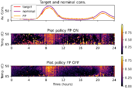
(a) Policy FP-MFG.

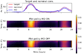
(b) Policy MD-MFC.

Figure 5: [top] Target, average consumption obtained by the nominal policy and by the policy computed by FP-MFG (left) and MD-MFC (right). [middle] Probability of choosing the ON action when in the ON state. [bottom] Probability of choosing the ON action when in the OFF state. For all temperatures between $T_{\text{min}}=50$ and $T_{\text{max}}=65$ [$y$ axis], over the course of a day with a time step of $10$ minutes [$x$ axis], for a target with a deviation step of eight hours.

(a) One hour step.

(b) Eight hours step.

Figure 6: Log-log plot of the objective function per iteration for each method when using a target with an one hour step [left] and eight hours step [right] deviations.

Different initialisations impact the number of switches

We noticed that different initialisations of MD-MFC lead to different policies. Given a state distribution sequence $\rho$, the policy generating this distribution is not necessarily unique. In particular, these policies, while providing the same $\rho$, may differ in terms of the average number of ON/OFF switches induced over the time horizon considered. In our model, no switching limit is assumed, but a large number of switches can be detrimental to the device. This non-uniqueness helps us reduce switch count without adding new constraints by finding multiple policies that achieve the right consumption and selecting the one with the fewest switches. This can also be useful for MFC problems in other areas, e.g. transaction costs in finance.

In the case illustrated here the average number of daily switches is $33$, while the nominal dynamic averages only $3$ switches per day. By initializing the MD-MFC algorithm with a policy that is a $0.1$ deviation from the nominal policy as in Figure 7(a), we find that the number of switches decreases to a daily average of $9.2$ while still following the target curve, see Figure 7(b). The same does not happen with FP-MFG, which makes it less interesting for the real-world scenarios we consider here.

Finally, Table 1 gives a global comparison between the three algorithms. FP-MFG converges faster but is not suitable for controlling switch count, being less interesting for the considered DSM problem, and needs a smooth objective function assumption. OMD-MFG is empirically as good as MD-MFC but lacks convergence proof for discrete cases.

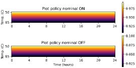
(a) Nominal policy deviation.

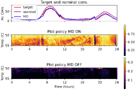
(b) Policy MD-MFC with nominal policy deviation.

Figure 7: [left] Initial policy sequence $\pi^{0}$ with a deviation of $0.1$ from the nominal policy. [right] Output policy sequence of Algorithm 1 initialized with the policy at left.

Table 1: Comparing MD-MFC, OMD-MFG and FP-MFG

Algorithm	Convergence rate	Flexibility on applications	Convergence hypothesis
MD-MFC	$K^{-1/2}$	Yes (switches)	convex + Lispschitz
OMD-MFG	no proof	Yes (switches)	convex + Lispschitz
FP-MFG	$K^{-1}$	No	convex + Lipschitz + smooth

5 Future work

Future work involves adapting existing algorithms to real-time algorithms, proposing schemes where each iteration corresponds to a time step. We further aim to generalize to a model-free scenario, learning user behavior on the fly while preserving privacy with partially observable states. Moreover, we believe we can extend our approach to the accelerated version of mirror descent [Krichene et al., 2015] providing a better theoretical convergence rate of order $1/K^{2}$.

Appendix A Missing proofs

A.1 Proof of Proposition 3.1

Proof.

Consider a fixed initial state-action distribution $\mu_{0}\in\Delta_{\mathcal{X}\times\mathcal{A}}$. Let $\mu\in\mathcal{M}_{\mu_{0}}$ and define $\rho=(\rho_{n})_{1\leq n\leq N}$ such that for all $x\in\mathcal{X}$, $\rho_{n}(x)=\sum_{a}\mu_{n}(x,a)$ (the associated state distribution). First, let us deal with the case where $\rho_{n}(x)\neq 0$. Define a policy sequence $\pi\in(\Delta_{\mathcal{A}})^{\mathcal{X}\times N}$ such that $\smash{\pi_{n}(a|x)=\frac{\mu_{n}(x,a)}{\rho_{n}(x)}}$ for all $(x,a)\in\mathcal{X}\times\mathcal{A}$. We want to show that $\mu^{\pi}=\mu$ for this policy $\pi$. We reason by induction. For $n=0$, $\mu_{0}^{\pi}=\mu_{0}$ by definition. Suppose $\mu^{\pi}_{n}=\mu_{n}$, thus for $n+1$ and for all $(x^{\prime},a^{\prime})\in\mathcal{X}\times\mathcal{A}$

$$\mu^{\pi}_{n+1}(x^{\prime},a^{\prime}) =\sum_{x,a}p_{n+1}(x^{\prime}|x,a)\mu_{n}^{\pi}(x,a)\pi_{n+1}(a^{\prime}|x^{\prime})$$

$$=\sum_{x,a}p_{n+1}(x^{\prime}|x,a)\mu_{n}(x,a)\frac{\mu_{n+1}(x^{\prime},a^{\prime})}{\rho_{n+1}(x^{\prime})}$$

$$=\sum_{a}\mu_{n+1}(x^{\prime},a)\frac{\mu_{n+1}(x^{\prime},a^{\prime})}{\rho_{n+1}(x^{\prime})}$$

$$=\rho_{n+1}(x^{\prime})\frac{\mu_{n+1}(x^{\prime},a^{\prime})}{\rho_{n+1}(x^{\prime})}$$

$$=\mu_{n+1}(x^{\prime},a^{\prime}),$$

where the first equality comes from Definition 2.1, the second equality comes from the induction assumption and the way we defined the strategy $\pi$, and the third comes from the assumption that $\mu\in\mathcal{M}_{\mu_{0}}$.

In the case $\rho_{n}(x)=0$, we therefore have $\mu_{n}(x,a)=0$ for all $a\in\mathcal{A}$, so any choice of $\pi_{n}(a|x)$ would work.

∎

Appendix B Missing proofs: algorithm 1 scheme and convergence rate

By abuse of notations, for any probability measure $\eta\in\Delta_{E}$ whatever the finite space $E$ on which it is defined we introduce the neg-entropy function, with the convention $0\log(0)=0$,

$$\phi(\eta):=\sum_{x\in E}\eta(x)\log\eta(x),$$

to which we associate the Bregman divergence $D$, also known as the KL divergence, such that for any pair $(\eta,\nu)\in\Delta_{E}\times\Delta_{E}$,

$$D(\eta,\nu):=\phi(\eta)-\phi(\nu)-\langle\phi^{\prime}(\nu),\eta-\nu\rangle.$$

Let $\rho_{n}$ denote the marginal probability distribution on $\mathcal{X}$ associated with $\mu_{n}$ i.e., for all $x\in\mathcal{X}$

$$\rho_{n}(x):=\sum_{a\in\mathcal{A}}\mu_{n}(x,a)\ .$$

Observe that to any $\mu=(\mu_{n})_{1\leq n\leq N}\in\mathcal{M}_{\mu_{0}}$ one can associate a unique probability mass function on $\mathcal{P}(\mathcal{X}\times\mathcal{A})^{N}$ denoted by $\mu_{1:N}$ such that $\mu_{1:N}$ is generated by the strategy $\pi=(\pi_{n})_{1\leq n\leq N}$ associated with $\mu$ which is determined by

$$\pi_{n}(a|x)=\frac{\mu_{n}(x,a)}{\rho_{n}(x)}\ ,$$

when $\rho_{n}(x)\neq 0$, otherwise we fix an arbitrary strategy $\pi_{n}(a|x)=\frac{1}{|\mathcal{A}|}$.

Before proving Theorems (3.2) and (3.3) we state and prove a Lemma which is key to proving both theorems.

Lemma B.1.

For any $\mu\in\mathcal{M}_{\mu_{0}}$ and $\mu^{\prime}\in\mathcal{M}_{\mu_{0}}^{*}$, with associated probability mass functions $\mu_{1:N},\mu^{\prime}_{1:N}\in\mathcal{P}\big{(}(\mathcal{X}\times\mathcal{A})^{N}\big{)}$ generated by $\pi,\pi^{\prime}$ respectively with the same initial state-action distribution, i.e. $\mu_{0}=\mu^{\prime}_{0}$, we have

$$\begin{split}D(\mu_{1:N},\mu^{\prime}_{1:N})&=\sum_{n=1}^{N}\mathbb{E}_{(x,a)\sim\mu_{n}(\cdot)}\left[\log\bigg{(}\frac{\pi_{n}(a|x)}{\pi^{\prime}_{n}(a|x)}\bigg{)}\right]\\ &={\displaystyle\sum_{n=1}^{N}D(\mu_{n},\mu^{\prime}_{n})-\sum_{n=0}^{N}D(\rho_{n},\rho^{\prime}_{n})}\end{split}$$ (10)

Proof.

For each $1\leq n\leq N$, let us define a transition matrix $P^{\pi_{n}}$ for all $x,x^{\prime}\in\mathcal{X}$ and $a,a^{\prime}\in\mathcal{A}$,

$$P^{\pi_{n}}(x^{\prime},a^{\prime}|x,a):=p_{n}(x^{\prime}|x,a)\pi_{n}(a^{\prime}|x^{\prime}).$$

Given Definition 2.1, for any randomized policy the state-action distributions evolve according to linear dynamics

$$\mu_{n}(x^{\prime},a^{\prime})=\langle\mu_{n-1}(\cdot),P^{\pi_{n}}(x^{\prime},a^{\prime}|\cdot)\rangle.$$

Any randomized policy $\pi$ gives a probability mass function $\mu_{1:N}$ that is Markovian:

$$\mu_{1:N}(\vec{y})=\mu_{0}(y_{0})P^{\pi_{1}}(y_{1}|y_{0})...P^{\pi_{N}}(y_{N}|y_{N-1}),$$ (11)

where $\vec{y}$ represents the elements of $(\mathcal{X}\times\mathcal{A})^{N+1}$ such that $y_{i}=(x_{i},a_{i})$ for all $0\leq i\leq N$. Note that $\mu_{n}(y_{n})$ is the marginal probability mass function.

Consider $\mu,\mu^{\prime}\in\mathcal{M}_{\mu_{0}}$ the state-action distribution sequences induced by $\pi,\pi^{\prime}$ respectively (i.e, $\mu=\mu^{\pi}$ and $\mu^{\prime}=\mu^{\pi^{\prime}})$. Thus, computing the relative entropy between the probability mass functions $\mu_{1:N},\mu^{\prime}_{1:N}$ gives

$$D(\mu_{1:N},\mu^{\prime}_{1:N}) =\sum_{\vec{y}}\mu_{1:N}(\vec{y})\log\left(\frac{\mu_{1:N}(\vec{y})}{\mu^{\prime}_{1:N}(\vec{y})}\right)$$

$$=\sum_{y_{0},...,y_{N}}\mu_{1:N}(\vec{y})\log\left(\frac{\mu_{0}(y_{0})P^{\pi_{1}}(y_{1}|y_{0})...P^{\pi_{N}}(y_{N}|y_{N-1})}{\mu^{\prime}_{0}(y_{0})P^{\pi^{\prime}_{1}}(y_{1}|y_{0})...P^{\pi^{\prime}_{N}}(y_{N}|y_{N-1})}\right)$$

$$=\sum_{y_{0},...,y_{N}}\mu_{1:N}(\vec{y})\sum_{i=1}^{N}\log\left(\frac{P^{\pi_{i}}(y_{i}|y_{i-1})}{P^{\pi^{\prime}_{i}}(y_{i}|y_{i-1})}\right).$$

Where

$$\sum_{i=1}^{N}\log\left(\frac{P^{\pi_{i}}(y_{i}|y_{i-1})}{P^{\pi^{\prime}_{i}}(y_{i}|y_{i-1})}\right) =\sum_{i=1}^{N}\log\left(\frac{p_{i}(x_{i}|x_{i-1},a_{i-1})\pi_{i}(a_{i}|x_{i})}{p_{i}(x_{i}|x_{i-1},a_{i-1})\pi_{i}^{\prime}(a_{i}|x_{i})}\right)$$

$$=\sum_{i=1}^{N}\log\left(\frac{\pi_{i}(a_{i}|x_{i})}{\pi_{i}^{\prime}(a_{i}|x_{i})}\right).$$

Thus,

$$D(\mu_{1:N},\mu^{\prime}_{1:N}) =\sum_{\vec{y}}\mu_{1:N}(\vec{y})\sum_{i=1}^{N}\log\left(\frac{\pi_{i}(a_{i}|x_{i})}{\pi_{i}^{\prime}(a_{i}|x_{i})}\right)$$

$$=\sum_{\vec{y}}\mu_{0}(y_{0})P^{\pi_{1}}(y_{1}|y_{0})...P^{\pi_{N}}(y_{N}|y_{N-1})\sum_{i=1}^{N}\log\left(\frac{\pi_{i}(a_{i}|x_{i})}{\pi_{i}^{\prime}(a_{i}|x_{i})}\right)$$

$$=\sum_{i=1}^{N}\sum_{x\in\mathcal{X}}\sum_{a\in\mathcal{A}}\mu_{i}(x,a)\log\left(\frac{\pi_{i}(a|x)}{\pi^{\prime}_{i}(a|x)}\right).$$

Where for the last equality we used that

$$\sum_{y_{0},...,y_{i-1}}\mu_{0}(y_{0})P^{\pi_{1}}(y_{1}|y_{0})...P^{\pi_{i}}(y_{i}|y_{i-1})=\sum_{y_{i}}\mu_{i}(y_{i})$$

and for a fixed $y_{i}$,

$$\sum_{y_{i+1},...,y_{N}}P^{\pi_{i+1}}(y_{i+1}|y_{i})...P^{\pi_{N}}(y_{N}|y_{N-1})=1.$$

This proves the first equality of the Lemma. We now prove the second. For this, we recall that Proposition 3.1 gives a unique relation between a state-action distribution sequence $\mu\in\mathcal{M}_{\mu_{0}}$ and the policy sequence $\pi\in(\Delta_{\mathcal{A}})^{\mathcal{X}\times N}$ inducing it by taking for all $1\leq i\leq N$, $(x,a)\in\mathcal{X}\times\mathcal{A}$,

$$\pi_{i}(a|x)=\frac{\mu_{i}(x,a)}{\rho_{i}(x)},\,$$

where $\rho$ is the marginal on the states of $\mu$. Using this relation, we have then that

$$\begin{split}D(\mu_{1:N},\mu^{\prime}_{1:N})&=\sum_{i=1}^{N}\sum_{x\in\mathcal{X}}\sum_{a\in\mathcal{A}}\mu_{i}(x,a)\log\bigg{(}\frac{\pi_{i}(a|x)}{\pi^{\prime}_{i}(a|x)}\bigg{)}\\ &=\sum_{i=1}^{N}\sum_{x\in\mathcal{X}}\sum_{a\in\mathcal{A}}\mu_{i}(x,a)\log\bigg{(}\frac{\mu_{i}(a|x)}{\rho_{i}(x)}\frac{\rho^{\prime}_{i}(x)}{\mu^{\prime}_{i}(a|x)}\bigg{)}\\ &=\sum_{i=1}^{N}\sum_{x\in\mathcal{X}}\sum_{a\in\mathcal{A}}\mu_{i}(x,a)\log\bigg{(}\frac{\mu_{i}(a|x)}{\mu^{\prime}_{i}(a|x)}\bigg{)}-\sum_{i=1}^{N}\sum_{x\in\mathcal{X}}\sum_{a\in\mathcal{A}}\mu_{i}(x,a)\log\bigg{(}\frac{\rho_{i}(x)}{\rho^{\prime}_{i}(x)}\bigg{)}\\ &=\sum_{i=1}^{N}\sum_{x\in\mathcal{X}}\sum_{a\in\mathcal{A}}\mu_{i}(x,a)\log\bigg{(}\frac{\mu_{i}(a|x)}{\mu^{\prime}_{i}(a|x)}\bigg{)}-\sum_{i=1}^{N}\sum_{x\in\mathcal{X}}\rho_{i}(x)\log\bigg{(}\frac{\rho_{i}(x)}{\rho^{\prime}_{i}(x)}\bigg{)}\\ &=\sum_{i=1}^{N}D(\mu_{i},\mu_{i}^{\prime})-\sum_{i=1}^{i}D(\rho_{i},\rho_{i}^{\prime})\end{split}$$

which concludes the proof. ∎

B.1 Proof of Theorem 3.2: formulation of Algorithm 1

Proof.

At each iteration we seek to solve

$$\begin{split}\mu^{k+1}\in\operatorname*{arg\,min}_{\mu^{\pi}\in\mathcal{M}_{\mu_{0}}}\bigg{\{}\langle\nabla F(\mu^{k}),\mu^{\pi}\rangle+\frac{1}{\tau_{k}}\sum_{n=1}^{N}\mathbb{E}_{(x,a)\sim\mu_{n}(\cdot)}\left[\log\bigg{(}\frac{\pi_{n}(a|x)}{\pi^{k}_{n}(a|x)}\bigg{)}\right]\bigg{\}}\,\end{split}$$ (12)

where recall that $\langle\nabla F(\mu^{k}),\mu^{\pi}\rangle:=\sum_{n=1}^{N}\langle\nabla f_{n}(\mu_{n}^{k}),\mu^{\pi}_{n}\rangle$. We further use that ${r_{n}(x_{n},a_{n},\mu_{n}):=-\nabla f_{n}(\mu_{n})(x_{n},a_{n})}$.

Now, we use the optimality principle to solve this optimization problem with an algorithm backward in time. Remember that the initial distribution $\mu_{0}$ is always fixed. The equivalence between solving a minimization problem on sequences of state-action distributions in $\mathcal{M}_{\mu_{0}}$ and on sequences of policies in $(\Delta_{\mathcal{A}})^{\mathcal{X}\times N}$ (see Proposition 3.1), allows us to reformulate Problem (12) on $\mathcal{M}_{\mu_{0}}$ into a problem on $(\Delta_{\mathcal{A}})^{\mathcal{X}\times N}$, thus

$$\begin{split}\eqref{MD_opt_problem_appendix}&=\max_{\pi\in(\Delta_{\mathcal{A}})^{\mathcal{X}\times N}}\bigg{\{}\sum_{n=0}^{N}\sum_{x,a}\mu_{n}^{\pi}(x,a)r_{n}(x,a,\mu_{n}^{k})\\ &\qquad-\frac{1}{\tau_{k}}\sum_{n=1}^{N}\sum_{x,a}\mu_{n-1}^{\pi}(x,a)\sum_{x^{\prime},a^{\prime}}p_{n}(x^{\prime}|x,a)\pi_{n}(a^{\prime}|x^{\prime})\log\left(\frac{\pi_{n}(a^{\prime}|x^{\prime})}{\pi_{n}^{k}(a^{\prime}|x^{\prime})}\right)\bigg{\}}\\ &=\max_{\pi\in(\Delta_{\mathcal{A}})^{\mathcal{X}\times N}}\bigg{\{}\sum_{n=0}^{N}\sum_{x,a}\mu^{\pi}_{n}(x,a)\bigg{[}r_{n}(x,a,\mu_{n}^{k})\\ &\qquad-\frac{1}{\tau_{k}}\sum_{x^{\prime},a^{\prime}}p_{n+1}(x^{\prime}|x,a)\pi_{n+1}(a^{\prime}|x^{\prime})\log\left(\frac{\pi_{n+1}(a^{\prime}|x^{\prime})}{\pi_{n+1}^{k}(a^{\prime}|x^{\prime})}\right)\bigg{]}\bigg{\}}\\ &=\max_{\pi\in(\Delta_{\mathcal{A}})^{\mathcal{X}\times N}}\bigg{\{}\mathbb{E}_{\pi}\bigg{[}r_{N}(x_{N},a_{N},\mu_{N}^{k})+\sum_{n=0}^{N-1}r_{n}(x_{n},a_{n},\mu_{n}^{k})\\ &\qquad-\frac{1}{\tau_{k}}\sum_{x^{\prime},a^{\prime}}p_{n+1}(x^{\prime}|x_{n},a_{n})\pi_{n+1}(a^{\prime}|x^{\prime})\log\left(\frac{\pi_{n+1}(a^{\prime}|x^{\prime})}{\pi_{n+1}^{k}(a^{\prime}|x^{\prime})}\right)\bigg{]}\bigg{\}}.\end{split}$$

Let us define a regularized version of the state-action value function that we denote by $\tilde{Q}^{k}$, such that for all $1\leq i\leq N$, $(x,a)\in\mathcal{X}\times\mathcal{A}$,

$$\begin{split}\tilde{Q}^{k}_{i}(x,a)&=\max_{\pi_{i+1:N}\in(\Delta_{\mathcal{A}})^{\mathcal{X}\times{N-i}}}\mathbb{E}_{\pi}\bigg{[}r_{N}(x_{N},a_{N},\mu_{N}^{k})+\sum_{n=i}^{N-1}\bigg{\{}r_{n}(x_{n},a_{n},\mu_{n}^{k})\\ &-\frac{1}{\tau_{k}}\sum_{x^{\prime},a^{\prime}}p_{n+1}(x^{\prime}|x_{n},a_{n})\pi_{n+1}(a^{\prime}|x^{\prime})\log\left(\frac{\pi_{n+1}(a^{\prime}|x^{\prime})}{\pi_{n+1}^{k}(a^{\prime}|x^{\prime})}\right)\bigg{\}}\bigg{|}(x_{i},a_{i})=(x,a)\bigg{]},\end{split}$$ (13)

where $\pi_{i+1:N}=\{\pi_{i+1},...,\pi_{N}\}$.

First, note that $\mathbb{E}_{(x,a)\sim\mu_{0}(\cdot)}[\tilde{Q}^{k}_{0}(x,a)]=$ (12). Moreover, the optimality principle states that this regularized state-action value function satisfies the following recursion

$$\begin{cases}\tilde{Q}_{N}(x,a)=r_{N}(x,a,\mu_{N}^{k})\\ \!\begin{aligned} \tilde{Q}_{i}(x,a)&=\max_{\pi_{i+1}\in(\Delta_{\mathcal{A}})^{\mathcal{X}}}\bigg{\{}r_{i}(x,a,\mu_{i}^{k})+\\ &\qquad\sum_{x^{\prime}}p_{i+1}(x^{\prime}|x,a)\sum_{a^{\prime}}\pi_{i+1}(a^{\prime}|x^{\prime})\left[-\frac{1}{\tau_{k}}\log\left(\frac{\pi_{i+1}(a^{\prime}|x^{\prime})}{\pi_{i+1}^{k}(a^{\prime}|x^{\prime})}\right)+\tilde{Q}_{i+1}(x^{\prime},a^{\prime})\right]\bigg{\}}.\end{aligned}\end{cases}$$

Thus, to solve (12) we compute backwards in time, i.e. for $i=N-1,...,0$, for all $x\in\mathcal{X}$,

$$\pi_{i+1}^{k+1}(\cdot|x)\in\operatorname*{arg\,max}_{\pi(\cdot|x)\in\Delta_{\mathcal{A}}}\left\{\big{\langle}\pi(\cdot|x),\tilde{Q}_{i+1}^{k}(x,\cdot)\big{\rangle}-\frac{1}{\tau_{k}}D\big{(}\pi(\cdot|x),\pi^{k}_{i+1}(\cdot|x)\big{)}\right\},$$

where $D$ is the KL divergence.

The solution of this optimisation problem for each time step $i$ can be found by writing the Lagrangian function $\mathcal{L}$ associated. Let $\lambda$ be the Lagrangian multiplier associated to the simplex constraint. For simplicity, let $\pi_{x}:=\pi(\cdot|x)$, $\pi_{x}^{k}:=\pi_{i+1}^{k}(\cdot|x)$ and $\tilde{Q}^{k}_{x}:=\tilde{Q}_{i+1}^{k}(x,\cdot)$. Thus,

$$\mathcal{L}(\pi_{x},\lambda)=\langle\pi_{x},\tilde{Q}^{k}_{x}\rangle-\frac{1}{\tau_{k}}D(\pi_{x},\pi_{x}^{k})-\lambda\left(\sum_{a\in\mathcal{A}}\pi_{x}(a)-1\right).$$

Taking the gradient of the Lagrangian with respect to $\pi_{x}(a)$ for each $a\in\mathcal{A}$ gives

$$\frac{\partial\mathcal{L}}{\partial\pi_{x}(a)}=\tilde{Q}^{k}_{x}(a)-\frac{1}{\tau_{k}}\log\left(\frac{\pi_{x}(a)}{\pi_{x}^{k}(a)}\right)-\frac{1}{\tau_{k}}-\lambda,$$

and thus

$$\begin{split}\frac{\partial\mathcal{L}}{\partial\pi_{x}(a)}=0\Longrightarrow\quad\pi_{x}(a)=\pi_{x}^{k}(a)\exp{\left(\tau_{k}\tilde{Q}_{x}^{k}(a)-1-\tau_{k}\lambda\right)}.\end{split}$$

Applying the simplex constraint, $\sum_{a\in\mathcal{A}}\pi_{x}(a)=1$, we find the value of the Lagrangian multipler $\lambda$, and we get for all $a\in\mathcal{A}$

$$\pi_{x}(a)=\frac{\pi_{x}^{k}(a)\exp{\left(\tau_{k}\tilde{Q}_{x}^{k}(a)\right)}}{\sum_{a^{\prime}\in\mathcal{A}}\pi_{x}^{k}(a^{\prime})\exp{\left(\tau_{k}\tilde{Q}_{x}^{k}(a^{\prime})\right)},}$$

which proves the theorem.

∎

B.2 Proof of Proposition 3.4

Proof.

Lemma B.1 states that

$$\Gamma(\mu,\mu^{\prime}):=\sum_{n=1}^{N}\mathbb{E}_{(x,a)\sim\mu_{n}(\cdot)}\left[\log\bigg{(}\frac{\pi_{n}(a^{\prime}|x^{\prime})}{\pi^{k}_{n}(a^{\prime}|x^{\prime})}\bigg{)}\right]={\displaystyle\sum_{t=0}^{n}D(\mu^{\prime}_{t},\mu_{t})-\sum_{t=0}^{n}D(\rho^{\prime}_{t},\rho_{t})}.$$

Recall that $\phi$ is the negentropy and that $D$ is the Bregman divergence induced by the negentropy. Define the function $\psi:(\Delta_{\mathcal{X}\times\mathcal{A}})^{N}\to\mathbb{R}$ such that

$$\psi(\mu):=\sum_{n=0}^{N}\phi(\mu_{n})-\sum_{n=0}^{N}\phi(\rho_{n}).$$

Note that for $\mu,\mu^{\prime}\in(\Delta_{\mathcal{X}\times\mathcal{A}})^{N}$ with marginals given by $\rho,\rho^{\prime}\in(\Delta_{\mathcal{X}})^{N}$, using the second equality of Lemma B.1,

$$\psi(\mu)-\psi(\mu^{\prime})-\langle\nabla\psi(\mu^{\prime}),\mu-\mu^{\prime}\rangle=\Gamma(\mu,\mu^{\prime}).$$

Thus, for $\Gamma$ to be a Bregman divergence it is sufficient to show that $\psi$ is a convex function. Recall that the marginal $\rho$ is such that for each $1\leq n\leq N$, and for all $x\in\mathcal{X}$, $\rho_{n}(x)=\sum_{a\in\mathcal{A}}\mu_{n}(x,a)$. Thus,

$$\begin{split}\psi(\mu)&=\sum_{n}\left[\sum_{x,a}\mu_{n}(x,a)\log(\mu_{n}(x,a))-\sum_{x}\rho_{n}(x)\log(\rho_{n}(x))\right]\\ &=\sum_{n}\sum_{x,a}\mu_{n}(x,a)\log\left(\frac{\mu_{n}(x,a)}{\sum_{a^{\prime}}\mu_{n}(x,a^{\prime})}\right).\end{split}$$

Computing the first order partial derivative of $\psi$ with respect to $\mu_{n}(x,a)$ for any $(x,a)\in\mathcal{X}\times\mathcal{A}$ and $1\leq n\leq N$, we get

$$\begin{split}\frac{\partial\psi}{\partial\mu_{n}(x,a)}(\mu)&=\log\left(\frac{\mu_{n}(x,a)}{\sum_{a^{\prime}}\mu_{n}(x,a^{\prime})}\right)+\mu_{n}(x,a)\frac{1}{\mu_{n}(x,a)}-\sum_{a^{\prime}}\mu_{n}(x,a^{\prime})\frac{1}{\sum_{a^{\prime}}\mu_{n}(x,a^{\prime})}\\ &=\log\left(\frac{\mu_{n}(x,a)}{\sum_{a^{\prime}}\mu_{n}(x,a^{\prime})}\right)\\ &=\log\left(\frac{\mu_{n}(x,a)}{\rho_{n}(x)}\right).\end{split}$$

Now we apply the following convexity property [Boyd and Vandenberghe, 2004]: $\psi$ is convex if and only if for all $\mu,\mu^{\prime}\in(\Delta_{\mathcal{X}\times\mathcal{A}})^{N}$, $\langle\psi^{\prime}(\mu)-\psi^{\prime}(\mu^{\prime}),\mu-\mu^{\prime}\rangle\geq 0$. Indeed,

$$\begin{split}\langle\psi^{\prime}(\mu)-\psi^{\prime}(\mu^{\prime}),\mu-\mu^{\prime}\rangle&=\sum_{n}\sum_{x,a}\left[\frac{\partial\psi}{\partial\mu_{n}(x,a)}(\mu)-\frac{\partial\psi}{\partial\mu_{n}(x,a)}(\mu^{\prime})\right]\big{(}\mu_{n}(x,a)-\mu^{\prime}_{n}(x,a)\big{)}\\ &=\sum_{n}\sum_{x,a}\left[\log\left(\frac{\mu_{n}(x,a)}{\rho_{n}(x)}\right)-\log\left(\frac{\mu^{\prime}_{n}(x,a)}{\rho^{\prime}_{n}(x)}\right)\right]\big{(}\mu_{n}(x,a)-\mu^{\prime}_{n}(x,a)\big{)}\\ &\overset{(a)}{=}\sum_{n}D(\mu_{n},\mu_{n}^{\prime})+D(\mu_{n},\mu^{\prime}_{n})-D(\rho_{n},\rho^{\prime}_{n})-D(\rho^{\prime}_{n},\rho_{n})\\ &\overset{(b)}{=}\Gamma(\mu,\mu^{\prime})+\Gamma(\mu^{\prime},\mu)\\ &\overset{(c)}{=}D(\mu_{1:N},\mu^{\prime}_{1:N})+D(\mu^{\prime}_{1:N},\mu_{1:N})\overset{(d)}{\geq}0,\end{split}$$

where $(a)$ comes from the definition of the KL divergence $D$, $(b)$ comes from the definition of $\Gamma$, $(c)$ comes from Lemma B.1 and $(d)$ comes from a property of Bregman divergences that they are always positive. As $\psi$ is convex and induces the divergence $\Gamma$ then $\Gamma$ is a Bregman divergence. After writing this proof, we came across a different strategy to prove that $\Gamma$ is a Bregman divergence that is presented in Appendix A of Neu et al. [2017].

Now we prove that $\Gamma$ is $1$-strongly convex with respect to the $\sup_{1\leq n\leq N}\|\cdot\|_{1}$ norm. By Lemma B.1,

$$\begin{split}\Gamma(\mu,\mu^{\prime})&=\sum_{n=1}^{N}D(\mu_{n},\mu_{n}^{\prime})-\sum_{n=1}^{N}D(\rho_{n},\rho^{\prime}_{n})\\ &=D(\mu_{1:N},\mu^{\prime}_{1:N})\\ &\geq 2\|\mu_{1:N}-\mu_{1:N}\|^{2}_{\textrm{TV}}\\ &=\frac{1}{2}\|\mu_{1:N}-\mu^{\prime}_{1:N}\|_{1}^{2},\end{split}$$

the last inequality being a consequence of Pinsker’s inequality. The norm $\|\cdot\|_{\text{TV}}$ stands for the total variation norm. Let $y$ represent an element of $(\mathcal{X}\times\mathcal{A})^{N+1}$ such that $y_{i}\in\mathcal{X}\times\mathcal{A}$ for all $1\leq i\leq N$. Observe that

$$\|\mu_{1:N}-\mu^{\prime}_{1:N}\|_{1} = \sum_{y\in(\mathcal{X}\times\mathcal{A})^{N+1}}|\mu_{1:N}(y)-\mu^{\prime}_{1:N}(y)|$$

$$\geq \sum_{y_{n}\in\mathcal{X}\times\mathcal{A}}\bigg{|}\sum_{y_{s}\in\mathcal{X}\times\mathcal{A}\,,\,s\neq n}\big{(}\mu_{1:N}(y)-\mu^{\prime}_{1:N}(y)\big{)}\bigg{|}$$

$$= \sum_{y_{n}\in\mathcal{X}\times\mathcal{A}}|\mu_{n}(y_{n})-\mu^{\prime}_{n}(y_{n})|\quad\textrm{for all}\ n\in\{1,\cdots,N\}.$$

In particular,

$$\|\mu_{1:N}-\mu^{\prime}_{1:N}\|_{1} \geq \sup_{1\leq n\leq N}\|\mu_{n}-\mu^{\prime}_{n}\|_{1}\ .$$

This implies that

$$\Gamma(\mu,\mu^{\prime}) \geq \frac{1}{2}\sup_{1\leq n\leq N}\|\mu_{n}-\mu^{\prime}_{n}\|_{1}^{2}\ ,$$

proving that $\Gamma$ is $1$-strongly convex with respect to the $\sup_{1\leq n\leq N}\|\cdot\|_{1}$ norm.

∎

B.3 Complements of the proof of Theorem 3.3

Proof.

Here we prove that if $(f_{n})_{1\leq n\leq N}$ are convex and Lipschitz with respect to the L$1$-norm, then so is $F$. Convexity: $F$ is convex as the sum of convex functions.

Lipschitz: Let $\mu,\mu^{\prime}\in(\mathcal{X}\times\mathcal{A})^{N}$. As $f_{n}$ is Lipschitz with respect to $\|\cdot\|_{1}$ with constant $l_{n}$, then $|f_{n}(\mu_{n})-f_{n}(\mu^{\prime}_{n})|\leq l_{n}\|\mu_{n}-\mu_{n}\|_{1}$ for all $1\leq n\leq N$. Therefore,

$$\begin{split}|F(\mu)-F(\mu^{\prime})|&=\bigg{|}\sum_{n=1}^{N}f_{n}(\mu_{n})-f_{n}(\mu^{\prime}_{n})\bigg{|}\\ &\leq\sum_{n=1}^{N}|f_{n}(\mu_{n})-f_{n}(\mu^{\prime}_{n})|\\ &\leq\sum_{n=1}^{N}l_{n}\|\mu_{n}-\mu_{n}^{\prime}\|_{1}\\ &\leq\bigg{(}\sum_{n=1}^{N}l_{n}^{2}\bigg{)}^{1/2}\bigg{(}\sum_{n=1}^{N}\|\mu_{n}-\mu^{\prime}_{n}\|_{1}^{2}\bigg{)}^{1/2}\\ &\leq L\|\mu-\mu^{\prime}\|_{1},\end{split}$$

where we use Cauchy-Schwarz in the second to last inequality. Therefore, $F$ is Lipschitz with respect to the L$1$-norm with constant ${L:=\big{(}\sum_{n=1}^{N}l_{n}^{2})^{1/2}.}$

∎

Appendix C Algorithms

Algorithm 2 Fictitious play for MFG (FP)

  Input: number of iterations K, initial policy $\pi^{0}$.

  Initialization: $\bar{\mu}^{0}=\mu^{\pi^{0}}$ as in Definition 2.1.

  for $k=0,...,K$ do

     $\pi^{k+1}\in\operatorname*{arg\,max}_{\pi}J(\pi,\bar{\mu}^{k})$, best response against $\bar{\mu}^{k}$.

     $\bar{\mu}^{k+1}=\frac{1}{k+1}\mu^{\pi^{k+1}}+\frac{k}{k+1}\bar{\mu}^{k}$.

  end for

  Return: $\bar{\mu}^{K}$ and $\bar{\pi}^{K}$ s.t. $\bar{\pi}^{K}_{n}(a|x):=\sum_{k=0}^{K}\frac{\rho^{\pi^{k}}_{n}(x)\pi_{n}^{k}(a|x)}{\sum_{k=0}^{K}\rho^{\pi^{k}}_{n}(x)}$, ($\rho_{n}^{\pi^{k}}(x):=\sum_{a\in\mathcal{A}}\mu_{n}^{\pi^{k}}(x,a)$ for all $k\leq K$).

Algorithm 3 Frank Wolfe

  Input: number of iterations K, initial distribution $\mu^{0}$, sequence $(\eta_{k})_{k}$.

  for $k=0,...,K$ do

     $\mu^{k}\in\operatorname*{arg\,min}_{\mu\in\mathcal{M}}\left\langle\mu,\nabla F(\bar{\mu}^{k})\right\rangle_{|\mathcal{X}\times\mathcal{A}|}$.

     $\bar{\mu}^{k+1}=(1-\eta_{k+1})\bar{\mu}^{k}+\eta_{k+1}\mu^{k}$.

  end for

  Return: $\bar{\mu}^{K}$

The Online Mirror Descent for MFG algorithm uses the regular state-value function (or $Q$-function) at each iteration. It’s definition is given by

$$\begin{split}Q_{n}^{\pi,\mu}(x,a)&:=\mathbb{E}_{\pi}\left[\sum_{i=n}^{N}r_{i}(x_{i},a_{i},\mu_{i})\bigg{|}x_{n}=x,a_{n}=a\right].\end{split}$$ (14)

Note that, considering an initial state-action distribution $\mu_{0}$, $J_{\mu_{0}}(\pi,\mu)=\mathbb{E}_{(x,a)\sim\mu_{0}}[Q^{\pi,\mu}_{0}(x,a)].$ Furthermore, $Q^{\pi,\mu}$ is the solution of the backward equation, for all $n<N$, $(x,a)\in\mathcal{X}\times\mathcal{A}$:

$$\begin{cases}Q^{\pi,\mu}_{N}(x,a)=r_{N}(x,a,\mu_{N})\\ \!\begin{aligned} Q_{n}^{\pi,\mu}&(x,a)=r_{n}(x,a,\mu_{n})+\sum_{x^{\prime}}p(x^{\prime}|x,a)\sum_{a^{\prime}}\pi_{n+1}(a^{\prime}|x^{\prime})Q_{n+1}^{\pi,\mu}(x^{\prime},a^{\prime}).\end{aligned}\end{cases}$$ (15)

Algorithm 4 OMD for MFG

  Input: number of iterations K, $\pi^{0}\in(\Delta_{\mathcal{A}})^{\mathcal{X}\times N}$.

  for $k=0,...,K$ do

     $\mu^{k}:=\mu^{\pi^{k}}$, as in Definition 2.1.

     $Q^{k}:=Q^{\pi^{k},\mu^{k}}$ as in Equation (15).

     $\pi_{n}^{k+1}(\cdot|x):=\operatorname*{arg\,max}_{\pi(\cdot|x)\in\Delta_{\mathcal{A}}}\langle Q_{n}^{k}(x,\cdot),\pi(\cdot|x)\rangle+\tau D\left(\pi(\cdot|x),\pi^{k}_{n}(\cdot|x)\right)$, $\forall x\in\mathcal{X},\forall n\leq N$.

  end for

  Return: $\mu^{K},\pi^{K}$

Appendix D Water heater application

D.1 Standard cycling behavior of one water heater

Let us consider a time window $[t_{0},t_{0}+T]$, and consider a discretisation of the time such that $t_{n}=t_{0}+n\delta_{t}$ for $n=0,...,N$, and $\delta_{t}=T/N$ the time frequency. At each time step $t_{n}$ (that for short we call $n$), the state of a water heater is described by a variable $X_{n}=(m_{n},\theta_{n})\in\{0,1\}\times\mathbb{R}^{+}$, where $m_{n}$ indicates the operating state of the heater (ON if $1$, OFF if $0$), and $\theta_{n}$ represents the average temperature of the water in the tank.

The evolution of the temperature in the next time step $t_{n+1}$ is given by $\theta_{n+1}=\bar{T}_{t_{n+1}}^{t_{n},m_{n},\theta_{n}}$, where $t\mapsto\bar{T}_{t}^{t_{n},m_{n},\theta_{n}}$ is the solution of the ordinary differential equation (ODE) in Equation (16) on the interval $[t_{n},t_{n+1}]$. This ODE models the impact of the heat loss to the environment temperature ($T_{\text{amb}}$), the Joule effect (heating) and water drains (hot water being withdrawn from the tanks for showers, taps, etc),

$$\begin{cases}\frac{dT(t)}{dt}=-\underbrace{\rho(T(t)-T_{\text{amb}})}_{\text{heat loss}}+\underbrace{\sigma m_{n}p_{\text{max}}}_{\text{Joule effect}}-\underbrace{\tau(T(t)-T_{\text{in}})f(t)}_{\text{water drain}}\\ T(t_{n})=\theta_{n}.\end{cases}$$ (16)

The parameters $\rho,\sigma,\tau$ are technical parameters of the water heater, $p_{\text{max}}$ is the maximum power, $T_{\text{in}}$ denotes the temperature of the cold water entering the tank, and $f(t)$ denotes the drain function.

The dynamics follow a cyclic ON/OFF decision rule with a deadband to ensure that the temperature is between a lower limit $T_{\text{min}}$ and an upper limit $T_{\text{max}}$. Thus, if the water heater is turned on, it heats water with the maximum capacity until its temperature exceeds $T_{\text{max}}$. Then, the heater turns off. The water temperature then decreases until it reaches $T_{\text{min}}$, then the heater turns on again and a new cycle begins. Therefore, the nominal dynamics at a discretized time is given by Equation (17) and is illustrated at Figure 1.

$$\begin{cases}\theta_{n+1}=\bar{T}_{t_{n+1}}^{t_{n},m_{n},\theta_{n}}\\ m_{n+1}=\begin{cases}m_{n},\quad\text{if}\;\theta_{n+1}\in[T_{\text{min}},T_{\text{max}}]\\ 0,\quad\text{if}\;\theta_{n+1}\geq T_{\text{max}}\\ 1,\quad\text{if}\;\theta_{n+1}\leq T_{\text{min}}.\end{cases}\end{cases}$$ (17)

Note that assuming the temperature set is finite prevents us from using the ODE on Equation (16) to compute the evolution of the mean temperature. In addition, we also have trouble computing the drain function $f(t)$, which in practice is not deterministic. Instead, we adapt this ODE to simplify our system. We start by making an Euler discretization of the ODE. We define a sequence $(d_{n})_{n}$ denoting the amount of draining in liters at each time step. To decide whether hot water is drawn at each time step, we also consider a sequence $(\epsilon_{n})_{n}$ of independent random variables following Bernoulli’s laws of parameters $(q_{n})_{n}$ respectively. The interest of having different parameters for each time step is to take into account the moments of the day when people are more inclined to use hot water (for taking a shower, doing the dishes, etc.). Assuming the existence of an independent water discharge at each time step is justified by assuming that the time frequency $\delta_{t}$ is large enough to contain all the time when hot water will be drawn from the water heater tank for a single use. In the interest of more realistic dynamics, we intend to weaken this assumption in future work. Therefore, we define

$$\begin{split}\theta^{\prime}_{n+1}=\theta_{n}+\delta_{t}\big{(}-\rho\left(\theta_{n}-T_{\text{amb}}\right)+\sigma m_{n}p_{\text{max}}-\epsilon_{n}\tau\left(\theta_{n}-T_{\text{in}}\right)d_{n}\big{)}.\end{split}$$ (18)

To tackle the finite-temperature state space problem, we assume that the space of possible temperatures $\Theta$ contains only integers from $T_{\text{amb}}$ (the room temperature) up to $T_{\text{max}}$, assuming that $T_{\text{amb}}<T_{\text{min}}$ (it is reasonable to assume that the ambient temperature is below the minimum temperature accepted for the heater). Given the dynamics of the operating state, $\theta_{n+1}$ never exceeds $T_{\text{max}}$ (the heater turns off when it reaches $T_{\text{max}}$ and when it is turned off, its temperature only decreases). On the other hand, drain may allow a temperature to be lower than $T_{\text{min}}$, but we assume that $T_{\text{amb}}$ is small enough that the mean temperature is never lower than it. Therefore, we can take $\theta_{n+1}=\text{Round}(\theta_{n+1}^{\prime})$, where

$$\text{Round}(\theta)=\begin{cases}\lfloor\theta\rfloor,\quad\text{if }B(\theta)=0\\ \lceil\theta\rceil,\quad\text{if }B(\theta)=1,\end{cases}$$

and $B(\theta)$ is a random variable following a Bernoulli of parameter $\theta-\lfloor\theta\rfloor$. Thus, the closer $\theta$ is to its smallest nearest integer, the greater the probability that we approximate $\theta$ by it, and vice-versa. We perform stochastic rounding instead of deterministic to have an unbiased temperature estimator, i.e. $\mathbb{E}[\theta_{n+1}]=\theta_{n+1}^{\prime}$.

D.2 Complements of the proof of Theorem 3.3 for the DSM problem

We show that the cost function considered in Problem (3) concerning the water heater optimisation problem is convex and Lipschitz with respect to the $L_{1}$ norm $\|\cdot\|_{1}$.

Convexity

for all $n\leq N$, each $f_{n}$ is given by

$$f_{n}(\mu_{n})=\left(\sum_{x,a}\mu_{n}(x,a)\varphi(x)-\gamma_{n}\right)^{2}.$$

Let $g$ be a real function such that $g(x)=(x-\gamma_{n})^{2}$. The function $g$ is convex and non-decreasing on $\mathbb{R}_{+}$.

Let $h:\mathbb{R}^{|\mathcal{X}\times\mathcal{A}|}\rightarrow\mathbb{R}$, such that ${h(\mu_{n})=\sum_{x,a}\mu_{n}(x,a)\varphi(x)}$. Note that ${\frac{\partial h}{\partial\mu_{n}(x,a)}(\mu_{n})=\varphi(x)}$. Thus, for any $\mu_{n},\mu_{n}^{\prime}\in\Delta_{\mathcal{X}\times\mathcal{A}}$,

$$h(\mu_{n})-h(\mu_{n}^{\prime})=\left(\sum_{x,a}\big{(}\mu_{n}(x,a)-\mu_{n}^{\prime}(x,a)\big{)}\varphi(x)\right)=\langle\nabla h(\mu_{n}^{\prime}),\mu_{n}-\mu_{n}^{\prime}\rangle,$$

therefore, the function $h$ is also convex. As $f_{n}(\mu_{n})=g(h(\mu_{n}))$, then $f_{n}$ is convex as $g$ and $h$ are convex, and $g$ is non decreasing in a univariate domain [Boyd and Vandenberghe, 2004].

Lipschitz

As $f_{n}$ is convex for all $1\leq n\leq N$, to show that it is Lipschitz with respect to the $\|\cdot\|_{1}$ norm, it suffices to show that the sup-norm $\|\cdot\|_{\infty}$ of $\nabla f_{n}$ is bounded (the sup-norm is the dual norm of the $L_{1}$ norm). This result can be found in Lemma $2.6$ of Shalev-Shwartz [2012].

For any $\mu_{n}\in\Delta_{\mathcal{X}\times\mathcal{A}}$,

$$\begin{split}\|\nabla f_{n}(\mu)\|&=\sup_{(x,a)\in\mathcal{X}\times\mathcal{A}}|\nabla f_{n}(\mu_{n})(x,a)|\\ &=2\sup_{(x,a)\in\mathcal{X}\times\mathcal{A}}|\mu_{n}(\varphi)-\gamma_{n}||\varphi(x)|\\ &=2\sup_{(x,a)\in\mathcal{X}\times\mathcal{A}}\bigg{|}\sum_{x^{\prime},a^{\prime}}\mu_{n}(x^{\prime},a^{\prime})\varphi(x^{\prime})-\gamma_{n}\bigg{|}|\varphi(x)|\\ &=2\sup_{x\in\mathcal{X}}|\langle\rho_{n},\varphi\rangle||\varphi(x)|\\ &\leq 2\|\varphi\|_{\infty}^{2}.\end{split}$$

Thus, $f_{n}$ is Lipschitz with respect to the $L_{1}$ norm with Lipschitz constant $l_{n}=2\|\varphi\|_{\infty}^{2}$. In our particular case $\varphi$ is bounded by $1$ (see its definition in Equation (2)), hence $l_{n}=2$ for all $1\leq n\leq N$.

D.3 Simulation of the nominal behavior of a water heater

Here we explain in details how the nominal dynamics are simulated in order to obtain the results in Section 4.2.

To simulate the nominal dynamics we use the nominal model presented in Equation (17) with the average temperature evolution introduced in Equation (18). To compute the sequences $(d_{n})_{n}$ and $(q_{n})_{n}$ regarding the amount of draining in liters and the probability of having a water withdrawal for each time step, respectively, we use data from the SMACH (Simulation Multi-Agents des Comportements Humains) platform [Albouys et al., 2019], which simulates power consumption of people in their homes separated by appliance. The data we use simulates the consumption of $5132$ water heaters at a time step of one minute over a week in the summer of $2018$.

Since we want a time step large enough to contain all the time that hot water will be drawn from the water heater tank for a single use, we take $\delta_{t}=10$ minutes instead of one minute (as initially provided by the data). Therefore we transform the data to contain for each water heater the average discharge over each $10$ minute interval. To compute $d_{n}$, we take the average discharge in liters over all water heaters with a water withdrawal during this time step. To calculate $(q_{n})_{n}$, we calculate the percentage of water heaters with a water withdrawal over the entire population for each time step. The values of the parameters $\rho,\sigma,\tau$ and $p_{\text{max}}$ are computed in Equation (19) using the variables introduced in Tables 2 and 3. We take $T_{\text{min}}=50^{\circ}C$, $T_{\text{max}}=65^{\circ}C$, $T_{\text{amb}}=25^{\circ}C$ and $T_{\text{in}}=18^{\circ}C$.

Table 2: Water heater intrinsic parameters.

Volume	$0.2$m3
Height	$1.37$m
EI (thickness of isolation)	$\frac{0.035}{4}$m
$p_{\text{max}}$	$3600*2200$W (in one hour)

Table 3: Other parameters specifications to compute Equation 19.

denWater (water density)	$1000$ kg m-3
capWater (water capacity)	$4185$ J kg-1 K-1
CI (heat conductivity)	$0.033$ W/(m K)
coefLoss (loss coeff.)	$\frac{\text{CI}}{\text{EI}}*2*3.14\sqrt{\frac{\text{vol}*3.14}{\text{height}}}$

$$\begin{split}\rho&=\frac{\text{coefLoss}*3600}{\text{capWater}*\text{denWater}*\text{vol/height}}\quad\text{(fraction of heat loss by hour)}\\ \sigma&=(\text{vol}*\text{denWater}*\text{capWater})^{-1}\\ \tau&=(\text{vol}*\text{denWater})^{-1}.\end{split}$$ (19)

Appendix E Potential games discussion

In Subsection 3.3 we mention an equivalence between the control Problem (3) and a game problem in order to be able to compare Algorithm 1 with learning algorithms for MFG in the literature. For this, we use results similar to those of Geist et al. [2022] and we refer to it for further definitions on a MFG structure and the notion of Nash equilibrium (NE).

In a mean field game problem, the goal of a representative player is to find a sequence of policies $\pi$ that maximises the expected sum of rewards when the population distributions sequence is given by $\mu:=(\mu_{n})_{1\leq n\leq N}$ and the initial state-action pair is sampled from a fixed distribution $\mu_{0}$,

$$\begin{split}J_{\mu_{0}}(\pi,\mu)&:=\mathbb{E}_{\pi}\left[\sum_{n=1}^{N}r_{n}(x_{n},a_{n},\mu_{n})\right].\end{split}$$ (20)

Let us define a game with the same transition probability $p$, and with reward defined as

$$r_{n}(x_{n},a_{n},\mu_{n}):=-\nabla f_{n}(\mu_{n})(x_{n},a_{n})$$ (21)

for all $(x_{n},a_{n},\mu_{n})\in\mathcal{X}\times\mathcal{A}\times\Delta_{\mathcal{X}\times\mathcal{A}}$.

Proposition E.1.

The strategy $\pi^{*}$ is a minimizer of Problem (3) if and only if, $(\mu^{\pi^{*}},\pi^{*})$ is a NE of the MFG defined with reward as in Equation (21). Furthermore, this game is monotone (and strictly monotone if $f_{n}$ is strictly convex for all $1\leq n\leq N$. See Definition E.2).

This Proposition connects the optimality conditions of Problem (3) and a NE, and shows that convexity and monotonicity are equivalent. If the optimization problem is (strictly) convex, the (unique) existence of an optimizer implies the (unique) existence of a NE. Thus, the notion of monotonicity when the reward depends on the state-action distribution provides the (unique) existence of a NE in the case of a potential game.

Proof.

The convexity of each $f_{n}$ for $1\leq n\leq N$, and the convexity of the set $\mathcal{M}_{\mu_{0}}$ ensure the existence of a minimizer of Problem (3) satisfying the optimality conditions. Also, Proposition 3.1 shows, for a fixed initial state-action distribution $\mu_{0}$, a surjection between the sets $(\Delta_{\mathcal{A}})^{\mathcal{X}\times N}$ and $\mathcal{M}_{\mu_{0}}$.

Let $(\mu^{*},\pi^{*})$, where $\mu^{*}=\mu^{\pi^{*}}$, be a Nash equilibrium.

By definition, a Nash equilibrium $(\mu^{*},\pi^{*})$ satisfies $\pi^{*}=\operatorname*{arg\,max}_{\pi}J(\pi,\mu^{*})$. In other words,

$$J(\pi^{*},\mu^{\pi^{*}})\geq J(\pi,\mu^{\pi^{*}})\quad\forall\pi\in(\Delta_{\mathcal{A}})^{\mathcal{X}\times N}.$$ (22)

Expanding the terms of the sum of expected rewards and using the definition of reward in a potential game, we obtain that

$$J(\pi,\mu^{\pi^{*}}) =\mathbb{E}_{\pi}\left[\sum_{n=1}^{N}r_{n}(x_{n},a_{n},\mu_{n}^{\pi^{*}})\right]$$

$$=\sum_{n=1}^{N}\sum_{x\in\mathcal{X},a\in A}r_{n}(x,a,\mu_{n}^{\pi^{*}})\mu_{n}^{\pi}(x,a)$$

$$=\sum_{n=1}^{N}-\left\langle\nabla f_{n}(\mu_{n}^{\pi^{*}}),\mu_{n}^{\pi}\right\rangle.$$

Similarly,

$$J(\pi^{*},\mu^{\pi^{*}})=\sum_{n=1}^{N}-\left\langle\nabla f_{n}(\mu_{n}^{\pi^{*}}),\mu_{n}^{\pi^{*}}\right\rangle.$$

Thus, the Nash equilibrium condition in Inequality (22) entails

$$\sum_{n=1}^{N}\big{\langle}\nabla f_{n}(\mu^{\pi^{*}}_{n}),\mu_{n}^{\pi^{*}}-\mu_{n}^{\pi}\big{\rangle}\leq 0.$$ (23)

As $f_{n}$ is convex for all $n\in\{1,...,N\}$, this yields

$$\sum_{n=1}^{N}f_{n}(\mu^{\pi^{*}}_{n})-f_{n}(\mu^{\pi}_{n})\leq 0.$$ (24)

Thus, $\pi^{*}$ satisfies the optimality conditions of Problem (3). We then proved that if $(\pi^{*},\mu^{*})$ is a NE with $\mu^{*}=\mu^{\pi^{*}}$, then $\pi^{*}$ is an optimum of Problem (3).

On the other way around, if $\pi^{*}$ is a minimizer of Problem (3) then it satisfies Inequality (24) for all $\pi\in(\Delta_{\mathcal{A}})^{\mathcal{X}\times N}$. Again, by convexity of $(f_{n})_{1\leq n\leq N}$, $\pi^{*}$ also satisfies Inequality (23). Following the same calculations backwards, we obtain that $\pi^{*}$ then satisfies Inequality (22), and by definition is then a NE. This concludes the first part of the proof.

The second part concerns the monotonicity of the game, defined below for the mean field game framework.

Definition E.2 (Monotonicity).

According to Lasry and Lions [2007], a game where the reward depends on the population’s state-action distribution (sometimes called “extended MFG” in the literature, see Gomes and Voskanyan [2016]) is (strictly) monotone if for any state-action distributions $\nu,\nu^{\prime}\in\Delta_{\mathcal{X}\times\mathcal{A}}$ with $\nu\neq\nu^{\prime}$,

$$\int_{\mathcal{X},\mathcal{A}}[r(x,a,\nu)-r(x,a,\nu^{\prime})]d(\nu-\nu^{\prime})(x,a)\leq 0,\;(<0).$$

Back to the proof, consider $\mu,\mu^{\prime}$ two distributions over $\mathcal{X}\times\mathcal{A}$. As the result should be true to all $n$, we omit the time step index for the computations. Recall that the reward is of the form $r(x,a,\mu)=-\nabla f(\mu)(x,a)$ for all $(x,a)\in\mathcal{X}\times\mathcal{A}$, with $f$ a convex function. Then,

$$\begin{split}\int_{\mathcal{X}\times\mathcal{A}}[r(x,a,\mu)-r(x,a,\mu^{\prime})]d(\mu-\mu^{\prime})(x,a)=&\int_{\mathcal{X}\times\mathcal{A}}[\nabla f(\mu^{\prime})(x,a)-\nabla f(\mu)(x,a)]d(\mu-\mu^{\prime})(x,a)\\ =&\left\langle\nabla f(\mu^{\prime})-\nabla f(\mu),\mu-\mu^{\prime}\right\rangle\leq 0\end{split}$$

where the last inequality comes from the convexity of $f$. ∎

References

• Foley et al. [2020] Jonathan Foley, Katherine Wilkinson, Chad Frischmann, Ryan Allard, João Gouveia, Kevin Bayuk, Mamta Mehra, Eric Toensmeier, Chris Forest, Tala Daya, Denton Gentry, Sarah Myhre, s. Karthik Mukkavilli, Abdulmutalib Yussuff, Ashok Mangotra, Phil Metz, Ariani Wartenberg, Chirjiv Anand, Marzieh Jafary, and Barbara Rodriguez. The Drawdown Review (2020) - Climate Solutions for a New Decade. 03 2020. doi: 10.13140/RG.2.2.31794.76487.
• RTE [2022] RTE. Futurs énergétiques 2050. Technical report, Le réseaux de transport d’électricité, 2022.
• Bakare et al. [2023] Mutiu Shola Bakare, Abubakar Abdulkarim, Mohammad Zeeshan, and Aliyu Nuhu Shuaibu. A comprehensive overview on demand side energy management towards smart grids: challenges, solutions, and future direction. Energy Informatics, 6(1):4, March 2023. ISSN 2520-8942. doi: 10.1186/s42162-023-00262-7. URL https://doi.org/10.1186/s42162-023-00262-7.
• Antonopoulos et al. [2020] Ioannis Antonopoulos, Valentin Robu, Benoit Couraud, Desen Kirli, Sonam Norbu, Aristides Kiprakis, David Flynn, Sergio Elizondo-Gonzalez, and Steve Wattam. Artificial intelligence and machine learning approaches to energy demand-side response: A systematic review. Renewable and Sustainable Energy Reviews, 130(C), 2020. URL https://ideas.repec.org/a/eee/rensus/v130y2020ics136403212030191x.html.
• Brégère et al. [2019] Margaux Brégère, Pierre Gaillard, Yannig Goude, and Gilles Stoltz. Target tracking for contextual bandits: Application to demand side management. In Kamalika Chaudhuri and Ruslan Salakhutdinov, editors, Proceedings of the 36th International Conference on Machine Learning, volume 97 of Proceedings of Machine Learning Research, pages 754–763. PMLR, 09–15 Jun 2019. URL https://proceedings.mlr.press/v97/bregere19a.html.
• López et al. [2019] Karol Lina López, Christian Gagné, and Marc-André Gardner. Demand-side management using deep learning for smart charging of electric vehicles. IEEE Transactions on Smart Grid, 10(3):2683–2691, 2019. doi: 10.1109/TSG.2018.2808247.
• Nemirovski and Yudin [1983] A Nemirovski and D Yudin. Problem complexity and Method Efficiency in Optimization. Wiley, New York, 1983.
• Bertsekas [2005] Dimitri P. Bertsekas. Dynamic Programming and Optimal Control, volume I. Athena Scientific, Belmont, MA, USA, 3rd edition, 2005.
• Albouys et al. [2019] Jérémy Albouys, Nicolas Sabouret, Yvon Haradji, Mathieu Schumann, and Christian Inard. SMACH: Multi-agent Simulation of Human Activity in the Household. In Yves Demazeau, Eric Matson, Juan Manuel Corchado, and Fernando De la Prieta, editors, Advances in Practical Applications of Survivable Agents and Multi-Agent Systems: The PAAMS Collection, pages 227–231, Cham, 2019. Springer International Publishing. ISBN 978-3-030-24209-1.
• Bušić and Meyn [2016] Ana Bušić and Sean Meyn. Distributed Randomized Control for Demand Dispatch. In 55th IEEE Conference on Decision and Control (CDC), Proceedings of 55th IEEE Conference on Decision and Control, December 2016.
• Jabin and Wang [2017] Pierre-Emmanuel Jabin and Zhenfu Wang. Mean Field Limit for Stochastic Particle Systems. In Nicola Bellomo, Pierre Degond, and Eitan Tadmor, editors, Active Particles, Volume 1 : Advances in Theory, Models, and Applications, pages 379–402. Springer International Publishing, Cham, 2017. ISBN 978-3-319-49996-3. doi: 10.1007/978-3-319-49996-3_10. URL https://doi.org/10.1007/978-3-319-49996-3_10.
• Shiri et al. [2019] Hamid Shiri, Jihong Park, and Mehdi Bennis. Massive autonomous uav path planning: A neural network based mean-field game theoretic approach. In 2019 IEEE Global Communications Conference (GLOBECOM), pages 1–6, 2019. doi: 10.1109/GLOBECOM38437.2019.9013181.
• Elamvazhuthi and Berman [2019] Karthik Elamvazhuthi and Spring Berman. Mean-field models in swarm robotics: a survey. Bioinspiration & Biomimetics, 15(1):015001, November 2019. doi: 10.1088/1748-3190/ab49a4. URL https://dx.doi.org/10.1088/1748-3190/ab49a4. Publisher: IOP Publishing.
• Achdou et al. [2014] Y Achdou, FJ Buera, JM Lasry, PL Lions, and B Moll. Partial differential equation models in macroeconomics. Philosophical transactions. Series A, Mathematical, physical, and engineering science, 2014. doi: 10.1098/rsta.2013.0397.
• Casgrain and Jaimungal [2018] Philippe Casgrain and Sebastian Jaimungal. Mean field games with partial information for algorithmic trading, 2018. URL https://arxiv.org/abs/1803.04094.
• De Paola et al. [2019] Antonio De Paola, Vincenzo Trovato, David Angeli, and Goran Strbac. A mean field game approach for distributed control of thermostatic loads acting in simultaneous energy-frequency response markets. IEEE Transactions on Smart Grid, 10(6):5987–5999, 2019. doi: 10.1109/TSG.2019.2895247.
• Bušić and Meyn [2019] Ana Bušić and Sean Meyn. Distributed control of thermostatically controlled loads: Kullback-leibler optimal control in continuous time. 2019 IEEE 58th Conference on Decision and Control (CDC), pages 7258–7265, 2019. doi: 10.1109/CDC40024.2019.9029603.
• Lee et al. [2021] Wonjun Lee, Siting Liu, Hamidou Tembine, Wuchen Li, and Stanley Osher. Controlling Propagation of Epidemics via Mean-Field Control. SIAM Journal on Applied Mathematics, 81(1):190–207, 2021. doi: 10.1137/20M1342690. URL https://doi.org/10.1137/20M1342690. _eprint: https://doi.org/10.1137/20M1342690.
• E et al. [2018] Weinan E, Jiequn Han, and Qianxiao Li. A mean-field optimal control formulation of deep learning. Research in the Mathematical Sciences, 6(1):10, December 2018. ISSN 2197-9847. doi: 10.1007/s40687-018-0172-y. URL https://doi.org/10.1007/s40687-018-0172-y.
• Ruthotto et al. [2020] Lars Ruthotto, Stanley J. Osher, Wuchen Li, Levon Nurbekyan, and Samy Wu Fung. A machine learning framework for solving high-dimensional mean field game and mean field control problems. Proceedings of the National Academy of Sciences, 117(17):9183–9193, 2020. doi: 10.1073/pnas.1922204117. URL https://www.pnas.org/doi/abs/10.1073/pnas.1922204117. _eprint: https://www.pnas.org/doi/pdf/10.1073/pnas.1922204117.
• Fouque and Zhang [2020] Jean-Pierre Fouque and Zhaoyu Zhang. Deep Learning Methods for Mean Field Control Problems With Delay. Frontiers in Applied Mathematics and Statistics, 6, 2020. ISSN 2297-4687. doi: 10.3389/fams.2020.00011. URL https://www.frontiersin.org/articles/10.3389/fams.2020.00011.
• Lin et al. [2021] Alex Tong Lin, Samy Wu Fung, Wuchen Li, Levon Nurbekyan, and Stanley J. Osher. Alternating the population and control neural networks to solve high-dimensional stochastic mean-field games. Proceedings of the National Academy of Sciences, 118(31):e2024713118, 2021. doi: 10.1073/pnas.2024713118. URL https://www.pnas.org/doi/abs/10.1073/pnas.2024713118.
• Ihara and Schweppe [1981] Satoru Ihara and Fred C. Schweppe. Physically based modeling of cold load pickup. IEEE Transactions on Power Apparatus and Systems, PAS-100(9):4142–4150, 1981. doi: 10.1109/TPAS.1981.316965.
• Malhame and Chong [1985] R. Malhame and Chee-Yee Chong. Electric load model synthesis by diffusion approximation of a high-order hybrid-state stochastic system. IEEE Transactions on Automatic Control, 30(9):854–860, 1985. doi: 10.1109/TAC.1985.1104071.
• Mortensen and Haggerty [1988] R.E. Mortensen and K.P. Haggerty. A stochastic computer model for heating and cooling loads. IEEE Transactions on Power Systems, 3(3):1213–1219, 1988. doi: 10.1109/59.14584.
• Kizilkale and Malhame [2013] Arman Kizilkale and Roland Malhame. Mean field based control of power system dispersed energy storage devices for peak load relief. In Proceedings of the IEEE Conference on Decision and Control, pages 4971–4976, 12 2013. ISBN 978-1-4673-5717-3. doi: 10.1109/CDC.2013.6760669.
• Kizilkale and Malhame [2014] Arman C. Kizilkale and Roland P. Malhame. Collective target tracking mean field control for markovian jump-driven models of electric water heating loads. IFAC Proceedings Volumes, 47(3):1867–1872, 2014. ISSN 1474-6670. doi: https://doi.org/10.3182/20140824-6-ZA-1003.00630. URL https://www.sciencedirect.com/science/article/pii/S1474667016418859. 19th IFAC World Congress.
• Cammardella et al. [2019] Neil Cammardella, Ana Bušić, Yuting Ji, and Sean Meyn. Kullback-leibler-quadratic optimal control of flexible power demand. In 2019 IEEE 58th Conference on Decision and Control (CDC), pages 4195–4201, 2019. doi: 10.1109/CDC40024.2019.9029512.
• Cammardella et al. [2021] Neil Cammardella, Ana Bušić, and Sean Meyn. Kullback-leibler-quadratic optimal control in a stochastic environment. In 2021 60th IEEE Conference on Decision and Control (CDC), pages 158–165, 2021. doi: 10.1109/CDC45484.2021.9682943.
• Lasry and Lions [2007] Jean-Michel Lasry and Pierre-Louis Lions. Mean field games. Japanese Journal of Mathematics, 2:229–260, 2007.
• Huang et al. [2006] Minyi Huang, Roland Malhame, and Peter Caines. Large population stochastic dynamic games: Closed-loop mckean-vlasov systems and the nash certainty equivalence principle. Commun. Inf. Syst., 6, 01 2006. doi: 10.4310/CIS.2006.v6.n3.a5.
• Bensoussan et al. [2013] Alain Bensoussan, Jens Frehse, and Phillip Yam. Mean field games and mean field type control theory, volume 101. Springer, 2013.
• Perrin et al. [2020] Sarah Perrin, Julien Perolat, Mathieu Lauriere, Matthieu Geist, Romuald Elie, and Olivier Pietquin. Fictitious Play for Mean Field Games: Continuous Time Analysis and Applications. In H. Larochelle, M. Ranzato, R. Hadsell, M. F. Balcan, and H. Lin, editors, Advances in Neural Information Processing Systems, volume 33, pages 13199–13213. Curran Associates, Inc., 2020. URL https://proceedings.neurips.cc/paper/2020/file/995ca733e3657ff9f5f3c823d73371e1-Paper.pdf.
• Pérolat et al. [2022] Julien Pérolat, Sarah Perrin, Romuald Elie, Mathieu Laurière, Georgios Piliouras, Matthieu Geist, Karl Tuyls, and Olivier Pietquin. Scaling up mean field games with online mirror descent. In Proceedings of the 39th International Conference on Machine Learning, ICML’22, 03 2022.
• Geist et al. [2022] Matthieu Geist, Julien Pérolat, Mathieu Laurière, Romuald Elie, Sarah Perrin, Oliver Bachem, Rémi Munos, and Olivier Pietquin. Concave utility reinforcement learning: The mean-field game viewpoint. In Proceedings of the 21st International Conference on Autonomous Agents and Multiagent Systems, AAMAS ’22, page 489–497, Richland, SC, 2022. International Foundation for Autonomous Agents and Multiagent Systems. ISBN 9781450392136.
• Frank and Wolfe [1956] Marguerite Frank and Philip Wolfe. An algorithm for quadratic programming. Naval Research Logistics Quarterly, 3(1-2):95–110, 1956. doi: https://doi.org/10.1002/nav.3800030109. URL https://onlinelibrary.wiley.com/doi/abs/10.1002/nav.3800030109.
• Beck and Teboulle [2003] Amir Beck and Marc Teboulle. Mirror descent and nonlinear projected subgradient methods for convex optimization. Oper. Res. Lett., 31(3):167–175, may 2003. ISSN 0167-6377. doi: 10.1016/S0167-6377(02)00231-6. URL https://doi.org/10.1016/S0167-6377(02)00231-6.
• Bonnans et al. [2021] J. Frédéric Bonnans, Pierre Lavigne, and Laurent Pfeiffer. Discrete potential mean field games: duality and numerical resolution, 2021. URL https://arxiv.org/abs/2106.07463.
• Krichene et al. [2015] Walid Krichene, Alexandre M. Bayen, and Peter L. Bartlett. Accelerated mirror descent in continuous and discrete time. In Proceedings of the 28th International Conference on Neural Information Processing Systems - Volume 2, NIPS’15, page 2845–2853, Cambridge, MA, USA, 2015. MIT Press.
• Boyd and Vandenberghe [2004] Stephen Boyd and Lieven Vandenberghe. Convex Optimization. Cambridge University Press, March 2004. ISBN 0521833787. URL http://www.amazon.com/exec/obidos/redirect?tag=citeulike-20&path=ASIN/0521833787.
• Neu et al. [2017] Gergely Neu, Anders Jonsson, and Vicenç Gómez. A unified view of entropy-regularized markov decision processes. In Deep Reinforcement Learning Symposium, NIPS’17, 05 2017.
• Shalev-Shwartz [2012] Shai Shalev-Shwartz. Online learning and online convex optimization. Found. Trends Mach. Learn., 4(2):107–194, feb 2012. ISSN 1935-8237. doi: 10.1561/2200000018. URL https://doi.org/10.1561/2200000018.
• Gomes and Voskanyan [2016] Diogo A. Gomes and Vardan K. Voskanyan. Extended deterministic mean-field games. SIAM Journal on Control and Optimization, 54(2):1030–1055, 2016. doi: 10.1137/130944503. URL https://doi.org/10.1137/130944503.