WHC: Weighted Hybrid Criterion for Filter Pruning on Convolutional Neural Networks

Abstract

Filter pruning has attracted increasing attention in recent years for its capacity in compressing and accelerating convolutional neural networks. Various data-independent criteria, including norm-based and relationship-based ones, were proposed to prune the most unimportant filters. However, these state-of-the-art criteria fail to fully consider the dissimilarity of filters, and thus might lead to performance degradation. In this paper, we first analyze the limitation of relationship-based criteria with examples, and then introduce a new data-independent criterion, Weighted Hybrid Criterion (WHC), to tackle the problems of both norm-based and relationship-based criteria. By taking the magnitude of each filter and the linear dependence between filters into consideration, WHC can robustly recognize the most redundant filters, which can be safely pruned without introducing severe performance degradation to networks. Extensive pruning experiments in a simple one-shot manner demonstrate the effectiveness of the proposed WHC. In particular, WHC can prune ResNet-50 on ImageNet with more than 42% of floating point operations reduced without any performance loss in top-5 accuracy.

Index Terms—  Filter pruning, CNN compression, acceleration.

1 Introduction

(a) Similar norms, different angles

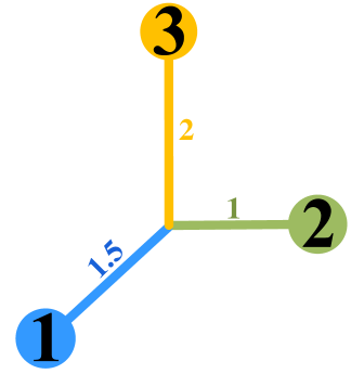
(b) Similar angles, different norms

Fig. 1: Examples in which relationship-based criteria lose efficacy.

Deep convolutional neural networks (CNNs) have achieved great success in various research fields in recent years, and broader or deeper architectures have been derived to obtain better performance [1]. However, state-of-the-art CNNs usually come with an enormously large number of parameters, costing prohibitive memory and computational resources, and thus are problematic to be deployed on resource-limited platforms such as mobile devices [2].

To tackle this problem, pruning methods, including weight pruning [3, 4] and filter pruning approaches [5, 6, 7], are developed to compress and accelerate CNNs. Weight pruning evaluates the importance of elements of weight tensors using criteria such as absolute value [3], and sets those with the lowest scores to zero to achieve element-wise sparsity. Nevertheless, as the sparsity is unstructured, weight pruning relies on customized software and hardware to accelerate CNNs. By contrast, filter pruning methods remove structured filters, which yields slimmer CNNs that can be applied to general-purpose hardware using the common BLAS libraries directly with less memory and inference time consumption, and thus have attracted more attention in recent years.

One of the core tasks in filter pruning is to avoid severe performance degradation on CNNs. To this end, many pruning criteria, including data-driven [8, 9, 10] and data-independent ones [11, 12], are proposed to find the most redundant filters, which can be safely deleted. In this paper, we focus on data-independent criteria, which can be further divided into two categories: norm-based [13] and relationship-based [12, 14, 15, 16]. The former believe that norms such as the $\ell_{1}$ and $\ell_{2}$ [11, 13] of filters indicate their importance, and thus prune filters with more minor norms. However, He et al. [14] argue that it is difficult for norm-based criteria to verify unimportant filters when the variance of norms is insignificant. To solve the problem, they propose a relationship-based criterion, FPGM, which prunes filters with the shortest Euclidean distances from the others. In line with FPGM, cosine criterion [15] and CFP [16] are also developed, in which filters with the highest angles and the weakest correlation with others are considered the most valuable, respectively.

Generally speaking, relationship-based methods can overcome the problems introduced by norm-based criteria but still have their imperfections. For example, considering the colored filters shown in Figure 1(a) with similar small norms but different angles, FPGM and the cosine distance criterion will delete the 1st filter while keeping the inverted 2nd and 3rd since they have the largest Euclidean or angle-wise distance with others. However, the 2nd and 3rd filters will extract strongly correlated (although negatively) feature maps that contain highly redundant information, while the 1st filter orthogonal to them may extract totally different features. Deleting the 1st filter will weaken the representative capacity of CNNs, therefore, it is the 2nd or 3rd filter that should be deleted instead of the 1st one. Furthermore, considering that the 2nd filter has a smaller norm than the 3rd one, it is more reasonable to prune the 2nd filter. Whereas, the cosine distance [15] and CFP  [16] criteria may rate the 2nd and 3rd the same score and remove one of them randomly. Similarly, this situation would also happen when filters have similar angles, such as the example shown in the Figure 1(b). These examples demonstrate that relationship-based criteria also need improvement.

In this paper, we propose a Weighted Hybrid Criterion (WHC) that considers both magnitude and relationship of filters to address the problems mentioned above and alleviate performance degradation robustly. Specifically, we value filters that have both more significant norms and higher dissimilarity from others (manifesting as orthogonality, instead of antiphase in FPGM [14] and cosine distance criterion [15]) while deleting the others. Moreover, we weigh filters’ dissimilarity terms differently rather than equally. That is, when evaluating a filter, its dissimilarity terms with filters of more significant norms are assigned a greater weight, while for filters of more minor norms, lower weights are appointed. The reason for this is that the dissimilarity evaluated by the degree of orthogonality is more trustworthy if the norm of a counterpart is more significant. In this manner, WHC can rationally score filters and prune those with the lowest scores, i.e., the most redundant ones, and thus alleviate the degradation in CNNs’ performance caused by pruning.

2 Methodology

2.1 Notation and Symbols

Weight tensors of a CNN. Following the conventions of PyTorch, we assume that a pre-trained $L$-layers CNN has weight tensors $\{\mathcal{W}_{l}\in\mathbb{R}^{N_{l+1}\times N_{l}\times K\times K}|l=1,2,\cdots,L\}$, where $\mathcal{W}_{l}$, $K\times K$, $N_{l}$ and $N_{l+1}$ stand for the weight tensor of the $l$-th convolutional layer, the kernel sizes, the number of input and output channels of the $l$-th convolutional layer, respectively.

Filters. We use $\mathcal{F}_{li}$ to represent the $i$-th filter of the $l$-th layer, where $\mathcal{F}_{li}=\mathcal{W}_{l}[i,:,:,:]\in\mathbb{R}^{N_{l}\times K\times K}$, i.e., the $i$-th slide of $\mathcal{W}_{l}$ along the first dimension.

Pruning rates. $r_{l}=\frac{\#\textrm{pruned filters}}{N_{l+1}}\in[0,1]$ denotes the proportion of pruned filters in the $l$-th layer.

2.2 Weighted Hybrid Criterion (WHC)

Norm-based criteria degrades when the variance of norms of filters is small [14], and relationship-based ones may fail to distinguish unimportant filters in several cases, as illustrated in Figure 1(a) and 1(b). To address these problems, we propose a data-independent Weighted Hybrid Criterion (WHC) to robustly prune the most redundant filters, which scores the importance of the $i$-th filter $\mathcal{F}_{li}$ in the $l$-th layer by taking into account not only the norm of a filter but also the linear dissimilarity as follows:

$${\textrm{score}}_{li}=\|\mathcal{F}_{li}\|_{2}\sum_{j=1,j\neq i}^{N_{l+1}}{\|\mathcal{F}_{lj}\|_{2}}\left(1-\lvert\cos{\theta_{i,j}}\rvert\right),$$ (1)

where

$$\cos{\theta_{i,j}}=\frac{<\mathcal{F}_{li},\mathcal{F}_{lj}>}{\|\mathcal{F}_{li}\|_{2}\cdot\|\mathcal{F}_{lj}\|_{2}},$$ (2)

and $\|\mathcal{F}_{ij}\|_{2}$ represents the $\ell_{2}$ norm of the vectorized $\mathcal{F}_{ij}$. Note that for a pre-trained model, we can assume that $\|\mathcal{F}_{lj}\|_{2}>0$.

When applying WHC in Eq. 1 for pruning, filters with lower scores are regarded as more redundant and thus will be deleted, while those with the opposite should be retained. To explain how WHC works in theory, we first discuss the unweighted variant of (1), Hybrid Criterion (HC):

$${\textrm{score}}_{li}^{\prime}=\|\mathcal{F}_{li}\|_{2}\sum_{j=1}^{N_{l+1}}\big{(}1-\lvert\cos{\theta_{i,j}}\rvert\big{)}.$$ (3)

Here $1-\lvert\cos{\theta_{i,j}}\rvert\in\left[0,1\right]$, the dissimilarity measurement (DM) between $\mathcal{F}_{li}$ and $\mathcal{F}_{li}$, acts as a scaling factor for $\|\mathcal{F}_{li}\|_{2}$, which in fact widens relative gaps between filters’ norms and thus tackles the problem of invalidation of norm-based criteria [14] caused by a small variance of norms. Moreover, unlike euclidean or angle-wise distance-based criteria [14, 15] that prefer filters having $180^{\circ}$ angles with others, WHC (1) and HC (3) value filters that are more orthogonal to the others, since they have shorter projected lengths with others and can extract less redundant features.

Note that in HC (3), the DM terms $1-\lvert\cos{\theta_{i,j}}\rvert$ for $j=1,\cdots,N_{l+1}$ are considered equally valuable. However, WHC has a different view: when evaluating a filter $\mathcal{F}_{li}$, weighs for the DM terms should be proportional to $\|\mathcal{F}_{lj}\|_{2}$ for $i\neq j$. The reason for this is that it is less robust to count on filters with smaller norms when scoring filters. To explain this, consider two orthogonal filters, $\mathcal{F}_{l1}=\left(100,0\right)$ and $\mathcal{F}_{l2}=\left(0,0.1\right)$. Since the norm of $\mathcal{F}_{l2}$ is minor, a small additive interference $\left(-0.1,-0.1\right)$ can easily change $\mathcal{F}_{l2}=(0,0.1)$ to $\mathcal{F}^{{}^{\prime}}_{l2}=(-0.1,0)$, which radically modifies the DM term of $\mathcal{F}_{l1}$ and $\mathcal{F}_{l2}$ from the ceiling 1 to the floor 0. To improve robustness, the DM term should be weighted.

AutoML techniques such as meta-learning [17] can be used to learn the weights, but it will be time-consuming. Alternatively, we directly take norms of filters as weights in WHC (1), such that the blind spots of norm-based and relationship-based criteria can be eliminated easily but effectively. As illustrated in Figure 2, when encountering the case shown in Figure 1(a) where norms of filters differ insignificantly, WHC can utilize dissimilarity information to score the filters and recognize the most redundant one. Furthermore, WHC is also robust to the case shown in Figure 1(b) in which the filters have similar linear relationships but with varied norms, while relationship-based criteria such as the cosine criterion [15] will lose effectiveness since it scores the filters equally. There is a scenario that WHC may lose efficacy, i.e., filters have the same norms and DM terms at the time. However, this indicates that there is no redundancy, and therefore it is not necessary to prune the corresponding model.

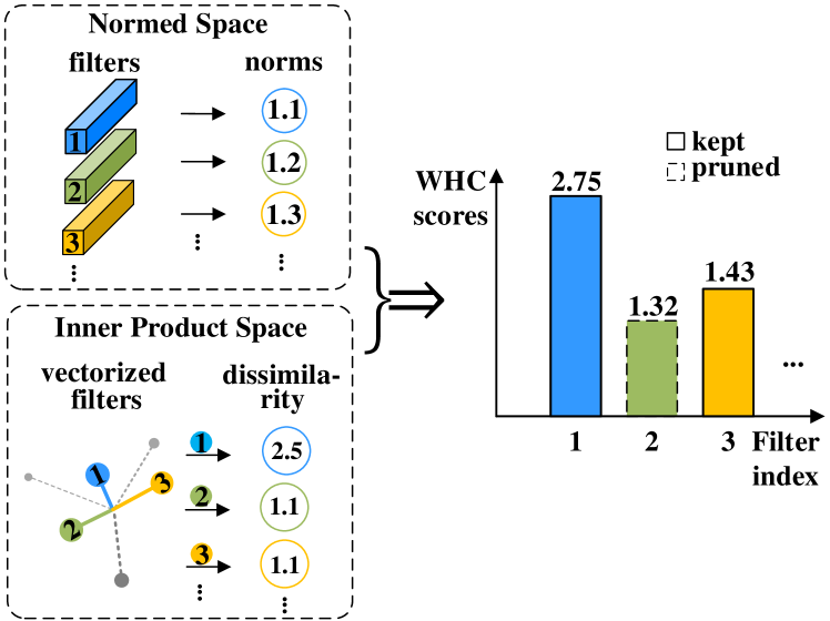
Fig. 2: Left top: Magnitude information of filters. Left bottom: Measuring dissimilarity of filters. Right: WHC scores filters and prune the most redundant ones.

2.3 Algorithm Description

As described in Algorithm 1, we perform filter pruning using WHC following the common “Pretrain-Prune-Finetune” pipeline in a simple single-shot manner, with all layers pruned under the same pruning rate, i.e., $r_{1}=r_{2}=\cdots=r_{L}$. Although iterative mechanism [18], Knowledge Distillation [19, 20, 21], sensitive analysis that decides layer-wise pruning rates [11], and some fine-tuning techniques [22] can improve the performance of pruned CNNs, none of them are included in this paper for ease of presentation and validation.

Algorithm 1 WHC for single-shot filter pruning

Input: Pre-trained model $\{\mathcal{W}_{l}\}_{l=1}^{L}$, pruning rates $r_{l}$, training data, fine-tuning epoch $epoch_{f}$

1:  for $l=L\rightarrow 1$ do

2:     Score $\{\mathcal{F}_{li}\}_{i=1}^{N_{l+1}}$ using WHC (1);

3:     Prune $r_{l}*N_{l+1}$ filters with the lowest scores to get $\mathcal{W}^{\prime}_{l}$;

4:     Replace $\mathcal{W}_{l}$ with $\mathcal{W}^{\prime}_{l}$.

5:  end for

6:  Fine-tune $\{\mathcal{W}^{\prime}_{l}\}_{l=1}^{L}$ for $epoch_{f}$ epochs.

Output: Compact model $\{\mathcal{W}^{\prime}_{l}\}_{l=1}^{L}$

By pruning $r_{l}\cdot N_{l+1}$ filters in the $l$-th layer, WHC also reduces the same number of input channels in the $l$+1-th layer. Suppose the input feature maps for the $l$-th layer are of dimensions $H_{l}\times W_{l}\times N_{l}$, and output feature maps for the $l$-th, $l$+1-th layer are of dimensions $H_{l+1}\times W_{l+1}\times N_{l+1}$ and $H_{l+2}\times W_{l+2}\times N_{l+2}$, respectively, pruning the $l$-th layer with $r_{l}$ will reduce $H_{l+1}W_{l+1}(N_{l+1}r_{l})K^{2}N_{l}+H_{l+2}W_{l+2}N_{l+2}K^{2}(N_{l+1}r_{l})$ floating point operations (FLOPs) totally, which greatly accelerates the forwarding inference.

3 Experiment

3.1 Experimental Settings

Datasets and baseline CNNs. Following [13, 14], we evaluate the proposed WHC on the compact and widely used ResNet-20/32/56/110 for CIFAR-10 [23] and ResNet-18/34/50/101 for ILSVRC-2012 (ImageNet) [24] For a fair comparison, we use the same pre-trained models for CIFAR-10 as [14]. Whereas, for ILSVRC-2012, since part of the per-trained parameters of [14] are not available, we use official Pytorch pre-trained models [25] with slightly lower accuracy. Code and CKPT are available at https://github.com/ShaowuChen/WHC.

Pruning and fine-tuning. The experiments are implemented with Pytorch 1.3.1 [25]. We keep all our implementations such as data argumentation strategies, pruning settings, and fine-tuning epochs the same as [13, 14], except that we use the straightforward single-shot mechanism. In the pruning stage, all convolutional layers in a network are pruned with the same pruning rate, and we report the proportion of “FLOPs” dropped for ease of comparison.

Compared methods. We compare WHC with several criteria, including the data-independent norm-based PFEC [11], SPF [13], ASPF [26], relationship-based FPGM [14], and several data-dependent methods HRank [27], GAL [28], LFPC [29], CP [30], NISP [31], ThiNet [18] and ABC [32].

Depth	Method	Baseline acc. (%)	Pruned acc. (%)	Acc. $\downarrow$ (%)	FLOPs $\downarrow$ (%)
20	WHC	92.20 ($\pm$0.18)	91.62 ($\pm$0.14)	0.58	42.2
	WHC	92.20 ($\pm$0.18)	90.72 ($\pm$0.16)	1.48	54.0
32	WHC	92.63 ($\pm$0.70)	92.71 ($\pm$0.08)	-0.08	41.5
	WHC	92.63 ($\pm$0.70)	92.44 ($\pm$0.12)	0.19	53.2
56	PFEC [11]	93.04	93.06	-0.02	27.6
	WHC	93.59 ($\pm$0.58)	93.91 ($\pm$0.06)	-0.32	28.4
	GAL [28]	93.26	93.38	0.12	37.6
	SFP [13]	93.59 ($\pm$0.58)	93.78 ($\pm$0.22)	-0.19	41.1
	WHC	93.59 ($\pm$0.58)	93.80 ($\pm$0.33)	-0.21	41.1
	HRank [27]	93.26	93.17	0.09	50.0
	SFP [13]	93.59 ($\pm$0.58)	93.35 ($\pm$0.31)	0.24	52.6
	ASFP [26]	93.59 ($\pm$0.58)	93.12 ($\pm$0.20)	0.47	52.6
	FPGM [14]	93.59 ($\pm$0.58)	93.26 ($\pm$0.03)	0.33	52.6
	WHC	93.59 ($\pm$0.58)	93.47 ($\pm$0.18)	0.12	52.6
	LFPC [29]	93.59 ($\pm$0.58)	93.24 ($\pm$0.17)	0.35	52.9
	ABC [32]	93.26	93.23	0.03	54.1
	WHC	93.59 ($\pm$0.58)	93.66 ($\pm$0.19)	-0.07	54.8
	GAL [28]	93.26	91.58	1.68	60.2
	WHC	93.59 ($\pm$0.58)	93.29 ($\pm$0.11)	0.30	63.2
110	GAL [28]	93.50	93.59	-0.09	18.7
	PFEC [11]	93.53	93.30	0.23	38.6
	SFP [13]	93.68 ($\pm$0.32)	93.86 ($\pm$0.21)	-0.18	40.8
	ASFP [26]	93.68 ($\pm$0.32)	93.37 ($\pm$0.12)	0.31	40.8
	WHC	93.68 ($\pm$0.32)	94.32 ($\pm$0.17)	-0.64	40.8
	GAL [28]	93.26	92.74	0.76	48.5
	SFP [13]	93.68 ($\pm$0.32)	92.90 ($\pm$0.18)	0.78	52.3
	FPGM [14]	93.68 ($\pm$0.32)	93.74 ($\pm$0.10)	-0.06	52.3
	ASFP [26]	93.68 ($\pm$0.32)	93.10 ($\pm$0.06)	0.58	52.3
	WHC	93.68 ($\pm$0.32)	94.07 ($\pm$0.20)	-0.39	52.3
	HRank [27]	93.50	93.36	0.14	58.2
	LFPC [29]	93.68 ($\pm$0.32)	93.07 ($\pm$0.15)	0.61	60.3
	ABC [32]	93.50	93.58	-0.08	65.0
	WHC	93.68 ($\pm$0.32)	93.82 ($\pm$0.07)	-0.14	65.8

Table 1: Pruning results on CIFAR-10. “$\downarrow$” means “drop”. In “Acc. $\downarrow$”, the smaller, the better; a negative drop means improvement. In “FLOPs $\downarrow$”, a larger number indicates that more FLOPs are reduced.

3.2 Evaluation on CIFAR-10

For CIFAR-10, we repeat each experiment three times and report the average accuracy after fine-tuning. As shown in Table 1, WHC outperforms several state-of-the-art counterparts. WHC can prune 52.3% of FLOPs in ResNet-110 with even 0.39% improvement, while the norm-based SFP under the same settings suffers 0.78% of degradation. The improvement shows that under moderate pruning rates, WHC can alleviate the overfitting problem of models without hurting their capacity.

Compared with the iterative ASFP [26], data-driven HRank [27], AutoML-based ABC [32] and LFPC [29], WHC in a single-shot manner can also achieve competitive performance. For example, although more FLOPs are reduced, WHC still achieves 0.42% and 0.75% higher accuracy than LFPC in ResNet-56 and ResNet-110, respectively, which demonstrates that WHC can recognize the most redundant filters effectively. Furthermore, under similar pruned rates, as the depth of CNNs increases, the pruned models obtained by WHC suffer less performance degradation. The reason for this is that deeper CNNs contain more redundancy, which can be removed by WHC robustly without hurting CNNs’ capacity severely.

Depth	Method	Baseline top-1 acc. (%)	Pruned top-1 acc. (%)	Top-1 acc. $\downarrow$ (%)	Baseline top-5 acc. (%)	Pruned top-5 acc. (%)	Top-5 acc. $\downarrow$ (%)	FLOPs $\downarrow$ (%)
18	SFP [13]	70.23	60.79	9.44	89.51	83.11	6.40	41.8
	ASFP [26]	70.23	68.02	2.21	89.51	88.19	1.32	41.8
	FPGM [14]	70.28	68.41	1.87	89.63	88.48	1.15	41.8
	WHC	69.76	68.48	1.28	89.08	88.52	0.56	41.8
34	PFEC [11]	73.23	72.17	1.06	-	-	-	24.2
	ABC [32]	73.28	70.98	2.30	91.45	90.05	1.40	41.0
	SFP [13]	73.92	72.29	1.63	91.62	90.90	0.72	41.1
	ASFP [26]	73.92	72.53	1.39	91.62	91.04	0.58	41.1
	FPGM [14]	73.92	72.54	1.38	91.62	91.13	0.49	41.1
	WHC	73.31	72.92	0.40	91.42	91.14	0.28	41.1
50	ThiNet [18]	72.88	72.04	0.84	91.14	90.67	0.47	36.7
	SFP [13]	76.15	62.14	14.01	92.87	84.60	8.27	41.8
	ASFP [26]	76.15	75.53	0.62	92.87	92.73	0.14	41.8
	FPGM [14]	76.15	75.59	0.56	92.87	92.63	0.24	42.2
	WHC	76.13	76.06	0.07	92.86	92.86	0.00	42.2
	HRank [27]	76.15	74.98	1.17	92.87	92.33	0.54	43.8
	NISP [31]	-	-	0.89	-	-	-	44.0
	GAL [28]	76.15	71.95	4.20	92.87	90.94	1.93	43.0
	CFP [16]	75.30	73.40	1.90	92.20	91.40	0.80	49.6
	CP [30]	-	-	-	92.20	90.80	1.40	50.0
	FPGM [14]	76.15	74.83	1.32	92.87	92.32	0.55	53.5
	WHC	76.13	75.33	0.80	92.86	92.52	0.34	53.5
	GAL [28]	76.15	71.80	4.35	92.87	90.82	2.05	55.0
	ABC [32]	76.01	73.86	2.15	92.96	91.69	1.27	54.3
	ABC [32]	76.01	73.52	2.49	92.96	91.51	1.45	56.6
	LFPC [29]	76.15	74.46	1.69	92.87	92.04	0.83	60.8
	WHC	76.13	74.64	1.49	92.86	92.16	0.70	60.9
101	FPGM [14]	77.37	77.32	0.05	93.56	93.56	0.00	42.2
	WHC	77.37	77.75	-0.38	93.55	93.84	-0.30	42.2
	ABC [32]	77.38	75.82	1.56	93.59	92.74	0.85	59.8
	WHC	77.37	76.63	0.74	93.55	93.30	0.25	60.8

Table 2: Pruning results on ILSVRC-2012 (ImageNet). “acc.” and “$\downarrow$” stand for ‘’accuracy” and “drop”, respectively.

3.3 Evaluation on ILSVRC-2012

The results are shown in Table 2. Not surprisingly, compared with several state-of-the-art methods, WHC not only achieves the highest top-1 and top-5 accuracy, but also suffers the slightest performance degradation. In ResNet-50, WHC reduces more than 40% of FLOPs but barely brings loss in the top-1 and top-5 accuracy, while the norm-based SFP suffers 14% degradation in the top-1 accuracy and other methods more than 0.5%. Compared with norm-based and relationship-based criteria, the superior performance of WHC can be attributed to the utilization of both norm and linear similarity information of filters, and the assigned weights on different DM terms can provide more robust results.

3.4 Ablation Study

Decoupling experiment. To further validate the effectiveness of WHC, we progressively decouple WHC into several criteria, as shown in Table 3. The cosine criterion [15] is also added for comparison. We repeat pruning 40% of filters in ResNet-32 and ResNet-56 three times and report the raw accuracy (without fine-tuning) and the average drop in accuracy after fine-tuning. Compared with the cosine criterion [15], the DM criterion suffers less degradation in accuracy and is therefore more rational. Taking into account both norm and dissimilarity, HC achieves better performance than $\ell_{2}$ and DM. Furthermore, by assigning different weights to the DM terms, WHC outperforms all counterparts stably, especially in the more compact ResNet-32. The $\ell_{2}$ achieves similar performance as WHC in ResNet-56, but fails to maintain the same performance in ResNet-32, demonstrating the robustness of the proposed WHC.

Depth& acc.	Criterion	Raw acc. (%)	Fine-tuned acc. $\downarrow$ (%)
32 92.63%	${\|{\mathcal{F}}_{li}\|_{2}}$ [13]	10.06	0.42
	${\sum_{j=1}^{N_{l+1}}\cos{\theta_{i,j}}}$ [15]	10.00	0.78
	${\sum_{j=1}^{N_{l+1}}(1-\lvert\cos{\theta_{i,j}}\rvert)}$ (DM)	11.30	0.56
	${\|\mathcal{F}_{li}\|_{2}\sum_{j=1}^{N_{l+1}}(1-\lvert\cos{\theta_{i,j}}\rvert)}$ (HC)	11.18	0.32
	${\|\mathcal{F}_{li}\|_{2}\sum_{j=1}^{N_{l+1}}\|\mathcal{F}_{lj}\|_{2}(1-\lvert\cos{\theta_{i,j}}\rvert)}$ (WHC)	11.25	0.19
56 93.59%	${\|{\mathcal{F}}_{li}\|_{2}}$ [13]	16.99	0.20
	${\sum_{j=1}^{N_{l+1}}\cos{\theta_{i,j}}}$ [15]	10.00	0.51
	${\sum_{j=1}^{N_{l+1}}(1-\lvert\cos{\theta_{i,j}}\rvert)}$ (DM)	9.94	0.37
	${\|\mathcal{F}_{li}\|_{2}\sum_{j=1}^{N_{l+1}}(1-\lvert\cos{\theta_{i,j}}\rvert)}$ (HC)	17.94	0.14
	${\|\mathcal{F}_{li}\|_{2}\sum_{j=1}^{N_{l+1}}\|\mathcal{F}_{lj}\|_{2}(1-\lvert\cos{\theta_{i,j}}\rvert)}$ (WHC)	19.73	0.12

Table 3: Decoupling results on ResNet-32 and ResNet-56 for CIFAR-10. “acc.” and “$\downarrow$” stand for “accuracy” and “drop”, respectively

Types of norm and dissimilarity measurement. We replace $\ell_{2}$ norm and $\cos{\theta_{i,j}}$ in WHC (1) with $\ell_{1}$ norm and correlation coefficient, respectively. The correlation can be regarded as the centralized version of $\cos{\theta_{i,j}}$. We conduct experiments on ResNet-32 with $r_{l}=40\%$, The fine-tuned accuracy of the $\ell_{1}$ and correlation version of WHC are $(92.50\pm 0.11)\%$ and $(92.62\pm 0.18)\%$, respectively, which are slightly higher than the naive WHC, $(92.44\pm 0.12)\%$. The results indicate that WHC can be further improved with more suitable types of norm and dissimilarity measurement.

3.5 Visualization

We prune 40% of filters in the first layer of ResNet-50 for ImageNet and visualize the output feature maps, as shown in Figure 3. Among the pruned filters, 3 and 34 can be replaced by 10 and 29, respectively, and [13,32,48,62, et al] fail to extract valuable features. We also compare WHC with the $\ell_{2}$ norm criterion [13] and relationship-based FPGM [14], finding that $\ell_{2}$ and FPGM rank the filters differently from WHC but finally give a similar pruning list under the given pruning rate. The only divergence of WHC and the $\ell_{2}$ criterion arises over filters 29 and 56: WHC keeps 29 and prunes 56, while $\ell_{2}$ criterion takes the opposite action. We consider filter 29 to be more valuable than filter 56, since the latter fails to extract significant features, while the former highlights the eyes of the input image. The difference of WHC and $\ell_{2}$ in the pruning list for a single layer is insignificant, but an accumulation of tens of layers finally results in a wide gap and makes WHC more robust in finding redundant filters.

(a) Input image

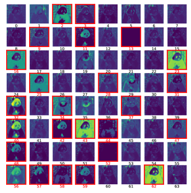
(b) Feature maps

Fig. 3: Visualization of ResNet-50-conv1 output feature maps (after ReLU, BN and MaxPooling, i.e., the input of the second Conv layer). The feature maps bounded by red boxes correspond to the pruned filters; 40% of the filters are pruned. The highest values are colored in the brightest green, while the lowest in the darkest blue.

4 Conclusion

We propose a simple but effective data-independent criterion, Weighted Hybrid Criterion (WHC), for filter pruning. Unlike previous norm-based and relationship-based criteria that use a single type of information to rank filters, WHC takes into consideration both magnitude of filters and dissimilarity between filter pairs, and thus can recognize the most redundant filters more efficiently. Furthermore, by reweighting the dissimilarity measurements according to the magnitude of counterpart filters adaptively, WHC is able to alleviate performance degradation on CNNs caused by pruning robustly.

References

- [1] Kaiming He, Xiangyu Zhang, Shaoqing Ren, and Jian Sun, “Deep residual learning for image recognition,” in CVPR, 2016, pp. 770–778.
- [2] Shaowu Chen, Jiahao Zhou, Weize Sun, and Lei Huang, “Joint matrix decomposition for deep convolutional neural networks compression,” Neurocomputing, 2022.
- [3] Song Han, Jeff Pool, John Tran, and William J. Dally, “Learning both weights and connections for efficient neural network,” in NeurIPS, 2015, pp. 1135–1143.
- [4] Jonathan Frankle and Michael Carbin, “The lottery ticket hypothesis: Finding sparse, trainable neural networks,” in ICLR, 2019.
- [5] S. H. Shabbeer Basha, Sheethal N. Gowda, and Dakala Jayachandra, “A simple hybrid filter pruning for efficient edge inference,” in ICASSP, 2022, pp. 3398–3402.
- [6] Zhuang Liu, Jianguo Li, Zhiqiang Shen, Gao Huang, Shoumeng Yan, and Changshui Zhang, “Learning efficient convolutional networks through network slimming,” in ICCV, 2017, pp. 2755–2763.
- [7] Yuan Zhang, Yuan Yuan, and Qi Wang, “ACP: adaptive channel pruning for efficient neural networks,” in ICASSP, 2022, pp. 4488–4492.
- [8] Jianbo Ye, Xin Lu, Zhe Lin, and James Z. Wang, “Rethinking the smaller-norm-less-informative assumption in channel pruning of convolution layers,” in ICLR, 2018.
- [9] Pavlo Molchanov, Arun Mallya, Stephen Tyree, Iuri Frosio, and Jan Kautz, “Importance estimation for neural network pruning,” in CVPR, 2019, pp. 11264–11272.
- [10] Shixing Yu, Zhewei Yao, Amir Gholami, Zhen Dong, Sehoon Kim, Michael W Mahoney, and Kurt Keutzer, “Hessian-aware pruning and optimal neural implant,” in WACV, 2022, pp. 3880–3891.
- [11] Hao Li, Asim Kadav, Igor Durdanovic, Hanan Samet, and Hans Peter Graf, “Pruning filters for efficient convnets,” in ICLR, 2017.
- [12] ZhaoJing Zhou, Yun Zhou, Zhuqing Jiang, Aidong Men, and Haiying Wang, “An efficient method for model pruning using knowledge distillation with few samples,” in ICASSP, 2022, pp. 2515–2519.
- [13] Yang He, Guoliang Kang, Xuanyi Dong, Yanwei Fu, and Yi Yang, “Soft filter pruning for accelerating deep convolutional neural networks,” in IJCAI, 2018, pp. 2234–2240.
- [14] Yang He, Ping Liu, Ziwei Wang, Zhilan Hu, and Yi Yang, “Filter pruning via geometric median for deep convolutional neural networks acceleration,” in CVPR, 2019, pp. 4340–4349.
- [15] Yang He, Ping Liu, Linchao Zhu, and Yi Yang, “Meta filter pruning to accelerate deep convolutional neural networks,” arXiv preprint arXiv:1904.03961, 2019.
- [16] Pravendra Singh, Vinay Kumar Verma, Piyush Rai, and Vinay P. Namboodiri, “Leveraging filter correlations for deep model compression,” in WACV, 2020, pp. 824–833.
- [17] Timothy M. Hospedales, Antreas Antoniou, Paul Micaelli, and Amos J. Storkey, “Meta-learning in neural networks: A survey,” IEEE Trans. Pattern Anal. Mach. Intell., vol. 44, no. 9, pp. 5149–5169, 2022.
- [18] Jian-Hao Luo, Jianxin Wu, and Weiyao Lin, “Thinet: A filter level pruning method for deep neural network compression,” in ICCV, 2017, pp. 5068–5076.
- [19] Haoli Bai, Hongda Mao, and Dinesh Nair, “Dynamically pruning segformer for efficient semantic segmentation,” in ICASSP, 2022, pp. 3298–3302.
- [20] ZhaoJing Zhou, Yun Zhou, Zhuqing Jiang, Aidong Men, and Haiying Wang, “An efficient method for model pruning using knowledge distillation with few samples,” in ICASSP, 2022, pp. 2515–2519.
- [21] Donggyu Joo, Eojindl Yi, Sunghyun Baek, and Junmo Kim, “Linearly replaceable filters for deep network channel pruning,” in AAAI, 2021, pp. 8021–8029.
- [22] Duong H. Le and Binh-Son Hua, “Network pruning that matters: A case study on retraining variants,” in ICLR, 2021.
- [23] Alex Krizhevsky and Geoffrey Hinton, “Learning multiple layers of features from tiny images,” Tech. Rep., 2009.
- [24] Olga Russakovsky, Jia Deng, Hao Su, Jonathan Krause, Sanjeev Satheesh, Sean Ma, Zhiheng Huang, Andrej Karpathy, Aditya Khosla, Michael S. Bernstein, Alexander C. Berg, and Li Fei-Fei, “Imagenet large scale visual recognition challenge,” Int. J. Comput. Vis., 2015.
- [25] Adam Paszke, Sam Gross, Soumith Chintala, Gregory Chanan, Edward Yang, Zachary DeVito, Zeming Lin, Alban Desmaison, Luca Antiga, and Adam Lerer, “Automatic differentiation in pytorch,” 2017.
- [26] Yang He, Xuanyi Dong, Guoliang Kang, Yanwei Fu, Chenggang Yan, and Yi Yang, “Asymptotic soft filter pruning for deep convolutional neural networks,” IEEE Trans. Cybern., pp. 3594–3604, 2020.
- [27] Mingbao Lin, Rongrong Ji, Yan Wang, Yichen Zhang, Baochang Zhang, Yonghong Tian, and Ling Shao, “Hrank: Filter pruning using high-rank feature map,” in CVPR, 2020, pp. 1526–1535.
- [28] Shaohui Lin, Rongrong Ji, Chenqian Yan, Baochang Zhang, Liujuan Cao, Qixiang Ye, Feiyue Huang, and David S. Doermann, “Towards optimal structured CNN pruning via generative adversarial learning,” in CVPR, 2019, pp. 2790–2799.
- [29] Yang He, Yuhang Ding, Ping Liu, Linchao Zhu, Hanwang Zhang, and Yi Yang, “Learning filter pruning criteria for deep convolutional neural networks acceleration,” in CVPR, 2020, pp. 2006–2015.
- [30] Yihui He, Xiangyu Zhang, and Jian Sun, “Channel pruning for accelerating very deep neural networks,” in ICCV, 2017, pp. 1398–1406.
- [31] Ruichi Yu, Ang Li, Chun-Fu Chen, Jui-Hsin Lai, Vlad I. Morariu, Xintong Han, Mingfei Gao, Ching-Yung Lin, and Larry S. Davis, “NISP: pruning networks using neuron importance score propagation,” in CVPR, 2018, pp. 9194–9203.
- [32] Mingbao Lin, Rongrong Ji, Yuxin Zhang, Baochang Zhang, Yongjian Wu, and Yonghong Tian, “Channel pruning via automatic structure search,” in IJCAI, 2020, pp. 673–679.