Cross-Validated Decision Trees with Targeted Maximum Likelihood Estimation for Nonparametric causal mixtures analysis

Abstract

Exposure to a mixture of chemicals such as drugs, pollutants and nutrients occur in most realistic exposure or treatment situations. We can imagine that, within this exposure space, there are arbitrary regions wherein we can measure the covariate adjusted outcome within the region compared to the complimentary exposure space. Ideally, it is most useful to estimate a causal estimand that maximizes this mean difference. A statistical estimator that identifies regions which maximize this difference and delivers the relevant effect unbiasedly would be valuable to public health efforts which aim to understand what levels of pollutants or drugs have the strongest effect. This estimator would take in as input a vector of exposures $A$ which can be a variety of data types (binary, multinomial, continuous), a vector of baseline covariates $W$ and outcome $Y$ and outputs 1. a region of the exposure space that attempts to optimize this maximum mean difference and 2. an unbiased estimate of the causal effect comparing the average outcomes if every unit were forced to self-select exposure within that region compared to the equivalent space outside of that region (the average regional-exposure effect (ARE)). Rather than the region of interest being of arbitrary shape, searching for rectangular regions is most helpful for policy implications by helping policymakers decide on what combination of thresholds to set on allowable combinations of exposures. This is because rectangular regions can be expressed as a series of thresholds, for example, $A_{1}\geq a_{1}$ while $A_{2}\leq a_{2}$ where $a_{1},a_{2}$ are specific doses of exposures $A_{1},A_{2}$ respectively. Non-parametric methods such as decision trees are a useful tool to evaluate combined exposures by finding partitions in the joint-exposure (mixture) space that best explain the variance in an outcome. We present a methodology for evaluating the causal effects of a data-adaptively determined mixture region using decision trees. This approach uses K-fold cross-validation and partitions the full data in each fold into a parameter-generating sample and an estimation sample. In the parameter-generating sample, decision trees are applied to a mixed exposure to obtain the region and estimators for our statistical target parameter. The region indicator and estimators are then applied to the estimation sample where the average regional-exposure effect is estimated. Targeted learning is used to update our initial estimates of the ARE in the estimation sample to optimize bias and variance towards our target parameter. This results in a plug-in estimator for our data-adaptive decision tree parameter that has an asymptotically normal distribution with minimum variance from which we can derive confidence intervals. Likewise, our approach uses the full data with no loss of power due to sample splitting. The open source software, CVtreeMLE, a package in R, implements our proposed methodology. Our approach makes possible the non-parametric estimation of the causal effects of a mixed exposure producing results that are both interpretable and asymptotically efficient. Thus, CVtreeMLE allows researchers to discover important mixtures of exposure and also provides robust statistical inference for the impact of these mixtures.

1 Introduction

In most environmental epidemiology studies, researchers are interested in how a joint exposure affects an outcome. This is because, in most real world exposure settings, an individual is exposed to a multitude of chemicals concurrently or, a mixed exposure. Individuals are exposed to a range of multi-pollutant chemical exposures from the environment including air pollution, endocrine disrupting chemicals, pesticides, and heavy metals. Because many of these chemicals may affect the same underlying biological pathway which lead to a disease state, the toxicity of these chemicals can be modified by simultaneous or sequential exposure to multiple agents. In these mixed exposure settings, the joint impact of the mixture on an outcome may not be equal to the additive effects of each individual agent. Mixed exposures may have impacts that are greater than expected given the sum of individual exposures or effects may be less than additive expectations if certain exposures antagonize the affects of others. Likewise, the effects of a mixed exposure may be different for subpopulations of individuals based on environmental stressors, genetic, and psychosocial factors that may modify the impact of a mixed exposure. Safe (1993); Kortenkamp (2007)

Causal inference of mixed exposures has been limited by reliance on parametric models and, in most cases, by researchers considering only one exposure at a time, usually estimated as a coefficient in a generalized linear regression model (GLM). This independent assessment of exposures poorly estimates the joint impact of a collection of the same exposures in a realistic exposure setting. Given that most researchers simply add individual effects to estimate the joint impact of an exposure, it is almost certain that the current evidence of the total impact environmental toxicants have on chronic disease is incorrectly estimated. The impact of using linear modeling is not limited to just potential bias: in the case where linearity does not hold, it’s not even clear what is being estimated.

The limitation in effective estimation of the joint effects of mixed exposure is (in-part) due to the lack of robust statistical methods. There has been some method development for estimation of joint effects of mixed exposures, such as Weighted Quantile Sum Regression Keil et al. (2019), Bayesian Mixture Modeling De Vocht et al. (2012), and Bayesian Kernel Machine Regression Bobb et al. (2014). However, these mixture methods have strong assumptions built into them, including directional homogeneity (e.g. all mixtures having a positive effect), linear/additive assumptions and/or require information priors. Many methods suffer from human bias due to choice of priors or poor model fit. More flexible models remain more or less a black-box and describe the mixture through a series of plots rather than with an interpretable summary statistic Bobb et al. (2014). Given that the National Institute for Environmental Health Sciences (NIEHS) has included the study of mixtures as a key goal in its 2018-2023 strategic plan National Institute of Environmental Health Sciences (2018) (NIEHS), it is imperative to develop new statistical methods for mixtures that are less biased, rely less on human input, use machine learning (ML) to model complex interactions, and are designed to return an interpretable parameter of interest.

Decision trees are a useful tool for outcome prediction based on exposures because they are fast, nonparametric (i.e. can discover and model interaction effects), and interpretable Leo Breiman (1984). However, it is not immediately clear how to adapt outcome prediction methods to inference about the effect of some kind of hypothetical intervention on the mixture of exposures- especially because in these settings we don’t have a particular intervention in mind.

Rather than leveraging decision trees for a simple prediction model, we introduce a target parameter on top of the prediction model, which is the average outcome within a fixed region of the exposure space. When an ensemble of decision trees is applied to an exposure mixture, this coincides with a leaf in the best fitting decision tree. By cross-estimating the average outcome given exposure to this region which maximizes the outcome difference we are able to build an estimator that is asymptotically unbiased with the smallest variance for our causal parameter of interest. Previous work, in the most naive approach, confidence intervals (CI) and hypothesis testing of decision trees is done by constructing a $(1-\alpha)\times 100$% confidence interval for a node mean $\bar{y}_{t}$ as $\bar{y}_{t}\pm±z_{1-\alpha/2}(\frac{s_{t}}{\sqrt{n_{t}}})$ where $\bar{y}_{t}$ is the node mean and $s_{t}$ is the standard deviation estimates in the node. Of course, these CI intervals tend to be overly optimistic because 1. decision trees are adaptive and greedy algorithms, meaning that they have a tendency to overfit and 2. the target parameter, in this case the node average, is estimated on the same data by which the node was created. Because of this the estimated CIs are too narrow. The best approach is to use an independent test set to derive inference for the expected outcome in each leaf. However, this approach is costly if additional data is gathered or power is greatly reduced if sample-splitting is done. Sampling splitting is done in previous work for causal inference of decision trees using so-called "honest estimation" for estimation of heterogeneous causal effects of a binary treatment. This approach Athey and Imbens (2016) uses one part of the data for constructing the partition nodes and and and another for estimating effects within leaves of the partition. Our proposed approach follows a similar sample-splitting technique where one part of the data is used to determine the partition nodes and the other is used to estimate the parameter of interest; however, we extend this technique to K-fold cross-validation where we rotate through the full data. Additionally, rather than estimating heterogenous treatment effects, we are interested in mapping a set of exposures that are of a variety of data types (continuous, binary, multinomial) into a set of partitioning rules using the best fitting decision tree from which we can estimate the average regional-exposure effect, or the expected outcome difference if all individuals were exposed to an exposure region compared to if no individuals were exposed to this region.

In most research scenarios, the analyst is interested in causal inference for an a priori specified treatment or exposure. However, in the evaluation of a mixed exposure it is not known what mixture components, levels of these components and combinations of these component levels contribute to the most to a change in the outcome. In the ideal scenario, the analyst has knowledge of the full, multidimensional dose-response curve $E[Y(A_{1},A_{2},...A_{k})]$ where $A$ are the exposures and $Y$ is the outcome. However, even in this case, it is difficult to estimate and/or interpret this curve. Estimation is hard because 1. we need unrealistic assumptions to get identifiability for the full curve and 2. the curve isn’t pathwise differentiable which means there aren’t any robust methods to build confidence intervals. Therefore, a sensible approach is to instead categorize the joint exposure and compare averages between categories as one would for a binary exposure. This approach is helpful because we can define interpretable categories like $(A_{1}>a_{1})\&(A_{2}<a_{2})$ where $a_{i}$ are specific values in $A$ (vs complement of this space) which are of clear interest to policymakers. Identification assumptions are also more transparent in this setting. However, we don’t know a priori what the right categorization of the exposure space are given some objective function. We have to use the data to tell us what regions are determined given a predefined objective function. In our case, we want a categorization that shows a maximal mean difference in outcomes. Regression trees are a nice way to do this while respecting the fact that we want interpretable rules like the above. The idea is to fit a kind of decision tree to figure out what thresholds in the exposure space produce a maximal exposure effect. As discussed, the result can be biased if we use the same data to define the thresholds and to estimate the effects in each leaf. We solve that problem by splitting the data, doing threshold estimation in one part and regional-exposure effect estimation (given the fixed thresholds) in the other. We can even redo the splits in a round-robin fashion (K-fold cross-validation) to efficiently use all of the data. Lastly, once we have thresholds, we want to get the best possible inference for the effect. We could always do a difference in outcome means between the samples in each category/region, but that estimate would be 1. biased by confounding and 2. have a large confidence interval because we haven’t used covariates to soak up residual variance. Our approach is thus to use a doubly-robust efficient estimator (TMLE) that simultaneously addresses both these problems.

Building on prior work related to data-adaptive parameters Hubbard et al. (2016) and cross-validated targeted minimum loss-based estimation (CV-TMLE) Zheng and van der Laan (2010), our method, called CVtreeMLE, is a novel approach for estimating the joint impact of a mixed exposure by using CV-TMLE which guarantees consistency, efficiency, and multiple robustness despite using highly flexible learners (ensemble machine learning) to estimate a data-adaptive parameter. CVtreeMLE summarizes the effect of a joint exposure on the outcome of interest by first doing an iterative backfitting procedure, similar to general additive models Hastie and Tibshirani (1990), to fit $f(A)$, a Super Learner van der Laan Mark et al. (2007) of decision trees, and $h(W)$, an unrestricted Super Learner, in a semi-parametric model; $E(Y|A,W)=f(A)+h(W)$, where $A$ is a vector of exposures and $W$ is a vector of covariates. In many public health settings, the analyst is first interested in a parsimonious set of thresholds focusing on the exposure space that best explains some outcome across the whole population rather partitions that also include baseline covariates. This additive model approach allows us to identify partitioning nodes in the exposure space while flexibly adjusting for covariates. In this way, we can data-adaptively find the best fitting decision tree model which has the lowest cross-validated model error while flexibly adjusting for covariates. This procedure is done to find partitions in the mixture space which allows for an interpretable mixture contrast parameter, "What is the expected difference in outcomes if all individuals were exposed to this region of the mixed exposure vs. if no individuals were exposed?". This approach easily extends to marginal case (partitions on individual exposures) as well. Our approach for integrating decision trees as a data-adaptive parameter with cross-validated targeted minimum loss-based estimation (CV-TMLE) allows for flexible machine learning estimators to be used to estimate nuisance parameter functionals while preserving desirable asymptotic properties of our target parameter. We provide implementations of this methodology in our free and open source software CVtreeMLE package, for the R language and environment for statistical computing [R Core Team, 2022].

This manuscript is organized as follows, in Section 2.1 we give a background of semi-parametric methodology, in section 2.2 we discuss the ARE target parameter for a fixed exposure region and in 2.3 the assumptions necessary for our statistical estimate to have a causal interpretation. In section 3 we discuss estimation and inference of the ARE for a fixed region. In section 4 we discuss data-adaptively determining the region which maximizes the W-controlled mean outcome difference. In section 5 we show how this requires cross-estimation which builds from 2.2 for a fixed region ARE. In section 5 we expand this to cross-estimation to k-fold CV and discuss methods for pooling estimates across the folds. Lastly, in section 5.3, because we may have different data-adaptively identified regions across the CV folds, we discuss the union rule which pairs with the pooled estimates. In section 6 we discuss simulations with two and three exposures and show our estimator is asymptotically unbiased with a normally sampling distribution. In section 7 we apply CVtreeMLE to the NIEHS mixtures workshop data and identify interactions built into the synthetic data. In section 7.1 we compare CVtreeMLE to the popular quantile sum g-computation method. In section 7.2 we apply CVtreeMLE to NHANES data to determine if there is association between mixed metals and leukocyte telomere length. Section 8 describes our CVtreeMLE software. We end with a brief discussion of the CVtreeMLE method in Section 9.

2 The Estimation Problem

2.1 Setup and Notation

Our setting is an observational study with baseline covariates ($W\in\mathbb{R}^{p}$), multiple exposures ($A\in\mathbb{R}^{m}$), and a single-timepoint outcome ($Y$). Let $O=(W,A,Y)$ denote the observable data. We presume that there exists a potential outcome function $Y(a)$ (i.e. $Y(a)$ is a random variable for each value of $a$) that generates the outcome that would have obtained for each observation had exposure been forced to the value $A=a$. These potential outcomes are unobserved but the observed outcome $Y$ corresponds to the potential outcome for the observed value $A$ of the exposure, i.e. $Y=Y(A)$. Let $E[Y(a)|W=w]=\mu(a,w)$ denote the causal dose-response curve for observations with covariates $w$ so that $E[\mu(a,W)]$ represents the average outcome we would observe if we forced treatment to $a$ for all observations.

We use $P_{0}$ to denote the data-generating distribution. That is, each sample from $P_{0}$ results in a different realization of the data and if sampled many times we would eventually learn the true $P_{0}$ distribution. We assume our $O_{1},O_{2},...,O_{n}$ are iid draws of $O=(W,A,Y)\sim P_{0}$. We decompose the joint density as $p_{Y,A,W}(y,a,w)=p_{Y|A,W}(y,a,w)p_{A|W}(a,w)p_{W}(w)$ and make no assumptions about the forms of these densities.

Compare this to to many methods which assume a parametric model which is one where each probability distribution $P\in\mathcal{M}$ can be uniquely described with a finite-dimensional set of parameters. Many methods assume $O$ to be identically distributed normal random variables, which means that the model can be described by the mean and standard deviation. Models like GLMs assume normal-linear relationships and assume $Y=X\beta+\mathcal{N}(\mu,\sigma^{2})$. Thus, methods for mixtures that use this approach have three parameters: the slope $\beta$, mean $\mu$ and standard deviation $\sigma$ of the normally-distributed random noise. This model assumes that the true relationship between $X$ and conditional mean of $Y$ is additive and linear and that the conditional distribution of $Y$ given $X$ is normal with a standard deviation that is fixed and doesn’t depend on $X$. Of course, these are very strict assumptions especially in the case of mixtures where exposures from a common source may be highly correlated, may interact on the outcome in a non-additive way, and may have non-normal distributions. As such, simply adding coefficients attached to variables in a mixture to estimate the overall joint effect may be biased.

Our statistical target parameter, $\Psi(P_{0})$, is defined as a mapping from the statistical model, $\mathcal{M}$, to the parameter space (i.e., a real number) $\mathbb{R}$. That is, $\Psi$: $\mathcal{M}\rightarrow\mathbb{R}$. We can think of this as, if $\Psi$ were given the true distribution $P_{0}$ it would provide us with our true estimand of interest.

We can think of our observed data $(O_{1}\dots O_{n})$ as a (random) probability distribution $P_{n}$ that places probability mass $1/n$ at each observation $O_{i}$. Our goal is to obtain a good approximation of the estimand $\Psi$, thus we need an estimator, which is an a-priori specified algorithm that is defined as a mapping from the set of possible empirical distributions, $P_{n}$ to the parameter space. More concretely, the estimator is a function that takes as input the observed data, a realization of $P_{n}$, and gives as output a value in the parameter space, which is the estimate, $\hat{\Psi}(P_{n})$. Since the estimator $\hat{\Psi}$ is a function of the empirical distribution $P_{n}$, the estimator itself is a random variable with a sampling distribution. So, if we repeat the experiment of drawing $n$ observations we would every time end up with a different realization of our estimate. We would like an estimator that is provably unbiased relative to the true (unknown) target parameter and which has the smallest possible sampling variance so that our estimation error is as small as it can be on average.

2.2 Defining the Differential Effect Given Regional Exposure

In problems with binary treatment $A\in\{0,1\}$ the standard counterfactual model defines potential outcomes $Y(0)$ and $Y(1)$ describing what would happen to each individual had they been forced onto either treatment. The estimand of interest is most often the average treatment effect $E[Y(1)]-E[Y(0)]$.

In our setting $A\in\mathbb{R}^{m}$ is continuous and we must thus define a potential outcome $Y(a)$ for each of the infinite possible values of the exposure. There is no singular, obvious “effect of treatment”.

In this work, we propose asking about the differential policy effect of allowing self-selection within a region of the exposure space. For example, we may be interested in the effect of a law that limits arsenic soil levels to a certain level while also limiting cadmium to a different level. In this setting, communities are still left to “self-select” exposures, but they must conform to the legal limits. In order to estimate such an effect, we have to specify how each individual would modify their “preference” for each exposure level when presented with a more limited set of choices. In this work we presume that relative self-selection preferences are preserved. For example, if a person were twice as likely to choose level $a_{1}$ as they were to choose $a_{2}$, that relative preference would continue to hold whether or not $a_{3}$ were a legal option. This is a special kind of modified treatment policy Hejazi et al. (2021, 2022); Iván Díaz Muñoz and Mark van der Laan* (2012).

Formally, let $\mathcal{A}\subset\mathbb{R}^{m}$ denote a subset of the exposure space. For example, presume that $\mathcal{A}$ represents dosages of drugs that have been deemed safe for combination. Let $\mathcal{A}$ also denote the binary random variable $1_{\mathcal{A}}(A)$ indicating whether an observation conformed to the policy. Let $\pi_{\mathcal{A}}(w)=P(A\in\mathcal{A}|W=w)$ be the probability that an observation with covariates $w$ naturally self-selects treatment in the requested region $\mathcal{A}$. We define the modified treatment variable $\tilde{A}$ to represent the distribution of exposure once all exposures are forced to be self-selected within the region $\mathcal{A}$. The modified treatment has density:

$$p_{\tilde{A}|W}(a,w)=\frac{1_{\mathcal{A}}(a)}{\pi_{\mathcal{A}}(w)}p_{A|W}(a,w)$$

which preserves the relative self-selection preferences for each available exposure and sets preferences for “outlawed” exposures to zero. Now we can define the population expected outcome ($\mu$) if we were to impose this policy:

$$E[\mu(\tilde{A},W)] =\int\mu(a,w)\,dP_{\tilde{A},W}$$

$$=\int\mu(a,w)\frac{1_{\mathcal{A}}(a)}{\pi_{\mathcal{A}}(w)}\,p_{A|W}(a,w)p_{W}(w)\,da\,dw$$

$$=\int_{w}\underbrace{\left[\int_{a\in\mathcal{A}}\mu(a,w)\frac{p_{A|W}(a,w)}{\pi_{\mathcal{A}}(w)}\ da\right]}_{Q(\mathcal{A}=1,w)}\ p_{W}(w)dw$$

$$=E[Q(\mathcal{A}=1,W)]$$

What we have shown is that this parameter is a population average of some function $m$ when $\mathcal{A}$ is forced to 1. For any value of $w$, $m(1,w)$ is a particular convexly weighted average of the causal dose-response curve across the different exposure levels, thus collapsing it down to a single number for each $w$.

In a similar fashion we define the population average outcome under the complementary policy $\mathcal{A}^{c}$, which is $E[Q(\mathcal{A}=0,W)]$. With this, we are ready to introduce our parameter of interest, which we call the average regional effect (ARE):

$$\psi^{*}=E[Q(\mathcal{A}=1,W)]-E[Q(\mathcal{A}=0,W)]$$

representing the difference in average outcomes if we forced exposure to self-selection within $\mathcal{A}$ vs. to self-selection within $\mathcal{A}^{c}$.

In most applications, it is not known a-priori what region $\mathcal{A}$ should be set. For example, we may not know how various chemicals or drugs interact and how to set safe limits for all of them. Therefore $\mathcal{A}$ itself is in practice something that should be estimated in order to maximize some objective. That said, for the purposes of establishing our theory we should first imagine $\mathcal{A}$ as known and fixed but depends on the original distribution of $A$. We will then show how we can choose what policy to enact (i.e. choose $\mathcal{A}$) while also unbiasedly estimating its effect.

2.3 Identification and Causal Assumptions

Our target parameter is defined on the causal data-generating process, so it remains to show that we can define it only in reference to observable quantities under certain assumptions. Standard conditioning arguments show that

$$\psi=E[E[Y|\mathcal{A}=1,W]-E[Y|\mathcal{A}=0,W]]$$

identifies the causal effect as long as the following assumptions hold:

1. Conditional Randomization: $A\perp Y(a)\mid W$ for all $a$

2. Positivity: $P(\mathcal{A}=1|W)>0$ for all $w$

Our identification result shows that we can get at the causal ARE by estimating an observable “ATE” under certain conditions. Our goal is now to show how to efficiently estimate the observable ATE without imposing any additional assumptions (e.g. linearity, normality, etc.). While our identification assumptions may not always hold in all applications, we can at least eliminate all model misspecification bias and minimize random variation. Once we’ve established how to estimate the ARE for a fixed region, we’ll turn our attention to the problem of finding a good region $\mathcal{A}$ and lastly how to do that without incurring selection bias in estimating the ARE for that region.

3 Estimating ARE with TMLE

In the previous sections we established that the causal ARE is equivalent to the observable ATE $E[E[Y|\mathcal{A}=1,W]-E[Y|\mathcal{A}=0,W]]$ under standard identifying assumptions. Therefore to estimate it all we need to do is 1) create a new binary random variable $\mathcal{A}_{i}=1_{\mathcal{A}}(A_{i})$ and 2) proceed as if we were estimating the observable ATE from the observational data structure $(Y,\mathcal{A},W)$.

There is an extensive literature on estimating the ATEs from observational data Nichols (2007); Winship and Morgan (1999); Rubin (2006). Using split-sample machine learning we can construct estimators that are provably unbiased (modulo bias from any violations of identifying assumptions), have the minimum possible sampling variance, and which are “doubly robust” Zheng and van der Laan (2010); Zivich and Breskin (2021). Augmented inverse propensity-weighting (AIPW) and targeted maximum likelihood (TMLE) are two established estimation approaches that accomplish these goals. Although they are usually very similar in practice, TMLE is often better for smaller samples Luque-Fernandez et al. (2018); Smith et al. (2022); van der Laan and Rose (2011, 2018) and should generally be preferred. In what follows we use the TMLE estimator of the ATE, which we briefly describe here.

The TMLE estimator is inspired by the fact that if we knew the true conditional mean $Q(\mathcal{A},W)=E[Y|\mathcal{A},W]$ we could estimate the ATE with the empirical average $\frac{1}{n}\sum_{i}Q(1,W_{i})-Q(0,W_{i})$. Of course, we do not know $Q$, but we can estimate it by regressing the outcome $Y$ onto the exposure $\mathcal{A}$ and covariates $W$. However a detailed mathematical analysis shows that we incur bias if we use our estimate $\hat{Q}$ instead of the truth. This bias might decrease as sample size increases, but it dominates relative to random variability, making it impossible to establish p-values or confidence intervals. TMLE solves this problem by computing a correction to the regression model $\hat{Q}$ that removes the bias. In other words, it “targets” the estimate $\hat{Q}$ to the parameter of interest (here the ATE). The process is as follows:

1. Use cross-validated ensembles of machine learning algorithms (a “super learner”) to generate estimates of the conditional means of treatment: $\hat{g}(\mathcal{A}=a,W)\approx P(\mathcal{A}=a|W)$ (i.e. propensity score) and outcome: $\hat{Q}(\mathcal{A},W)\approx E[Y|\mathcal{A},W]$

2. Regress $Y$ (scaled to $[0,1]$) onto the “clever covariate” $H_{i}=\frac{1_{1}(\mathcal{A}_{i})}{\hat{g}(1,W_{i})}-\frac{1_{0}(\mathcal{A}_{i})}{\hat{g}(0,W_{i})}$ using a logistic regression with a fixed offset term $\text{logit}(\hat{Q}(\mathcal{A},X))$. The (rescaled) output of this is our targeted regression model $\hat{Q}^{*}$

3. Compute the plug-in estimate using the targeted model: $\hat{\psi}=\frac{1}{n}\sum_{i}\hat{Q}^{*}(1,W_{i})-\hat{Q}^{*}(0,W_{i})$

An estimated standard error for $\hat{\psi}$ is given by

$$\hat{\sigma}^{2}=\frac{1}{n^{2}}\sum_{i}\left[\left(\frac{1_{1}(\mathcal{A}_{i})}{\hat{g}(1,W_{i})}-\frac{1_{0}(\mathcal{A}_{i})}{\hat{g}(0,W_{i})}\right)\bigg{(}Y_{i}-\hat{Q}^{*}(\mathcal{A}_{i},W_{i})\bigg{)}+\bigg{(}\hat{Q}^{*}(1,W_{i})-\hat{Q}^{*}(0,W_{i})\bigg{)}-\hat{\psi}\right]^{2}$$

with corresponding 95% confidence interval $\hat{\psi}\pm 1.96\hat{\sigma}$.

Explaining why the targeting step takes the form of a logistic regression and how the estimated standard error is derived are beyond the scope of this work. van der Laan and Rubin (2006); van der Laan and Rose (2011, 2018) offer explanations targeted to audiences with varying levels of mathematical sophistication.

To obtain these estimates we need only to specify the ensemble of machine learning algorithms used to estimate the propensity and initial outcome regressions $\hat{g}$ and $\hat{Q}$. The theoretical guarantees hold as long as a sufficiently rich library is chosen.

For estimating the ARE, we must also specify the region $\mathcal{A}$ so that we can compute our binary “exposure” variable. The issue of course is that we have been treating $\mathcal{A}$ as a known region, whereas in many applications the important question is figuring out what guidelines to impose in the first place. This is the focus of the next section.

4 Defining the Target Region

Thus far we have not focused on how we define the target region $\mathcal{A}$. First, let’s think of $\mathcal{A}$ as nonparametrically defined as the maximizer of some criterion, independent of an estimator. We can think of this as any region on the exposure gradient that maximizes the outcome (can take any shape). However, such a region isn’t interpretable. Therefore, it is easier to constrain the optimization so $\mathcal{A}$ is a rectangle in the exposure space. This is because these sections can be easily described using $\geq$ and $\leq$ rules. This is also important from a public health standpoint where these rules effectively are thresholds of exposures found to have the most severe (or least severe) affects. For this purpose, regression trees are an ideal estimator to get at such a region. Each decision tree algorithm uses some objective function to split a node into two or more sub-nodes. Of course, it is generally impossible to know a priori which learner will perform best for a given prediction problem and data set. Decision trees have many hyper-parameters such as the maximum depth, minimum samples in a leaf, and criteria for splitting amongst others. As such, we need to find the decision tree estimator that best fits the data given a set of nodes. We do this by creating a library of decision tree estimators to be applied to the exposure data and use cross-validation to select nodes based on the best fitting decision tree. This CV selection of the best fitting decision tree algorithm defines our exposure Super Learner $f(A)$ in our additive semi-parametric model $E(Y|A,W)=f(A)+h(W)$. This additive model is needed because we are interested in finding regions that maximize an outcome within only an exposure space not including the baseline covariates.

4.1 Discovering Regions in Multiple Exposures using Ensemble Trees

To discover regions in multiple exposures and therefore discover interactions in the exposure space, we use predictive learning via rule ensembles Friedman and Popescu (2008). Thus, as part of the data-adaptive procedure the $f(A)$ is a regression model constructed as a linear combinations of simple rules derived from the exposure data. Each rule consists of a conjunction of a small number of simple statements concerning the values of individual input exposures. Machine learning using rule ensembles have not only been shown to have predictive accuracy comparable to the best methods but also result in a linear combination of interpretable rules. Prediction rules used in the ensemble are logical if [conditions] then [prediction] statements, which in our case the conditions are regions in the exposure space that are predictive of the outcome. Learning ensembles have the structure:

$$F(x)=a_{0}+\sum_{m=1}^{M}a_{m}f_{m}(x)$$

where $M$ is the size of the ensemble (total number of trees) and each ensemble member $f_{m}(x)$ is a different function of the input exposures $A$ derived from the training data in the cross-estimation procedure (discussed later). Ensemble predictions from $F(x)$ are derived from a linear combination of the predictions of each ensemble member with ${a_{m}}_{0}^{M}$ being the parameters specifying the linear combination. Given a set of base learners, trees constructed using the exposures, ${{f_{m}(x)}_{1}^{M}}$ the parameters for the linear combination are obtained by a regularized linear regression using the training data. Ideally, each tree in the ensemble is limited to including only 2-3 exposures at a time which enhances interpretability. For instance, given the noise and small sample size in most public health studies, it is unlikely that signal is strong enough to detect interactions with 4 or more variables. Not only that but trees with partitions across many variables become less interpretable. Therefore, in our case we are interested in using an ensemble algorithm that creates a linear combination of smaller trees but also shows optimal prediction performance. To accomplish this goal we use the PRE package Fokkema (2020a) which is similar to the original RuleFit algorithm Friedman and Popescu (2008) with some enhancements including 1. unbiased recursive partitioning algorithms, 2. complete implementation in R, 3. capacity to handle many outcome types and 4. includes a random forest approach to generating prediction rules in addition to bagging and boosting methods. Here, the package PRE is fit to the exposure data in the training sample. Mechanically the procedure is 1. generate an ensemble of trees using exposure data, 2. fit a lasso regression using these trees to predict the outcome, 3. extract the tree basis with nonzero coefficients, 4. store these basis as rules which when evaluated on the exposure space demarcate an exposure region $\mathcal{A}$. There may then be many exposure regions such as $\mathcal{A}_{X_{1},X_{2}}$ which is a region including exposures $X_{1},X_{2}$ or another region in the exposure space which uses variables $X_{4},X_{5}$, $\mathcal{A}_{X_{4},X_{5}}$ etc. The ARE is then calculated for each of these regions which are based off of trees found to be predictive in the ensemble. In the case that multiple trees are included in the ensemble which are composed of the same set of exposures, we select the tree with the largest coefficient. This procedure is done in each fold of the cross-validation procedure.

4.2 Discovering Regions in Single Exposures using Decision Trees

In addition to finding interactions in the exposure space, the analyst may also be interested in identifying what exposures have a marginal impact and at what levels the outcome changes the most in these exposures. To answer this question we include a marginal tree fitting procedure which is very similar to the method described in 4.1. Here, $f(A)$ is a Super Learner of decision trees fit onto one exposure at a time. We then extract the rules determined from the best fitting tree. Each terminal leaf demarcates a region in the exposure and thus similarly we may have several $\mathcal{A}$ for 1 exposure which are the regions found when creating the partitions which best explains the outcome. Here, rather than calculating an ARE for each region we calculate an ARE comparing each region to the reference region. The reference region is defined as the region that captures the lowest values of $A$. For example, consider our resulting decision tree when fit to variable $A_{1}$ resulted in terminal leaves $A_{1}<0.6$, $A_{1}>0.6$ & $A_{1}<0.9$, $A_{1}>0.9$, in this case the reference region would be $A_{1}<0.6$. We would then have two ARE estimates for the two regions above the reference region. Mechanically, in the training sample, we find the best fitting decision tree which finds partitions in one exposure that best explains an outcome, these rules are evaluated as if statements on the exposure to create $\mathcal{A}_{i}=1_{\mathcal{A}}(A_{i})$ for the respective exposure. We then subset the reference level out and row bind it with each region above the reference region and pass that data to our estimators of the ARE. This approach was chosen to give users a dose-response type estimate for data-adaptively determined thresholds in the univariate exposure space.

4.3 Iterative Backfitting

We need an algorithm that will allow us to fit $f(A)$ while controlling for $W$ but not including $W$ in the partitions (trees). As such, we iteratively backfit two Super Learners $f(A)$ a Super Learner of decision trees and $h(W)$ an unrestricted Super Learner applied to the covariates. However, both algorithms need to use the same convergence criteria (here maximum likelihood estimation). Thus, $f(A)$ uses an ensemble of regression trees and $h(W)$ uses an ensemble of flexible MLE based algorithms (MARS, elastic net, Highly Adaptive Lasso amongst others). The algorithm first initializes by getting predictions from $f(A)$ and $h(W)$, that is, simply fitting a Super Learner to the exposures and covariates separately and then getting predictions. Then we begin fitting each algorithm offset by the predictions of the other. So at iteration 1 we fit $f(A,\text{offset}=h(W)_{\text{iter 0}})$ and likewise $h(W,\text{offset}=f(A)_{\text{iter 0}})$; where the offsets are predictions of the models fit individually (without offset at iteration 0). The predictions of these models without an offset then gives us $f(A)_{\text{iter 1}}$ and $h(W)_{\text{iter 1}}$. These predictions are then used as offsets at iteration 2. This process continues until convergence where convergence is is defined as the absolute mean difference between the two models being less than some very small number $\delta$ where $\delta$ by default is 0.001. In this way, for both where $A$ in $f(A)$ is a vector of exposures (resulting rules include combinations of different exposure levels) and when $A$ is a single exposure, we are able to identify cut-points in the exposure space while controlling for $W$ in the additive model that converges in maximum likelihood. We evaluate the best fitting decision tree onto the exposure space which results in an indicator of the exposure region and calculate our k-fold specific and pooled target parameters give this region.

4.4 Convergence to the True Region

The cross-validation selector is simply the recursive partitioning algorithm which performed best in terms of cross-validated risk within the parameter-generating sample. Assuming that a partition $\{\mathcal{D}_{d}\}d=1,...,D$ of the space $A=A_{1},...,A_{Z}$ exists with $D$ cells (or segments) such that the $\mathcal{D}_{d}$ cells are used to define the $\mathcal{A}$ boundaries, then the oracle selector as defined in Theorem 2 of van der Laan et al. (2008) is the estimator, among the decision tree learners considered, which minimizes risk under the true data-generating distribution $P_{0}$. That is, the oracle selector is the best possible estimator given the set of candidate decision tree learners considered; however, it of course depends on both the observed data and $P_{0}$, and thus is unknown. Theorem 2 in van der Laan et al. (2008) shows that the Super Learner performs as well (in terms of expected risk difference) as the oracle selector, up to a typically second order term. Therefore, as long as the number of candidate decision tree learners considered is polynomial in sample size ($n^{x}$), the Super Learner is the optimal learner. Given that the Super Learner performs asymptotically as well (in the risk difference sense) as the oracle selector, which chooses the best of the decision tree candidate learners, and given that, this class of learners are restricted to algorithms which partition the mixture space into $\mathcal{D}_{d}$ nodes of finite depth, it follows then that the selection of $\mathcal{D}_{d}$ nodes used in the decision tree estimator selected by the Super Learner converges asymptotically to the $\mathcal{D}_{d}$ nodes used by the oracle selector under depth constraints. Here the finite tree depth is needed because without tree depth limits, as sample size increases the best fitting estimator will always be the decision tree with increased depth and therefore there is no convergence to some true set of $\mathcal{D}_{d}$ nodes. Likewise, for interpretability, we are interested in some small set of nodes, or thresholds, per variable that is informative for public policy. That is to say, we may limit the ensemble of decision trees to a depth of 3 for interpretability. For example, we may want a more concise rule such as, "if arsenic is greater than X and lead is greater than Y", or without monotonic assumptions, "if arsenic is between X1 and X2 and lead is between Y1 and Y2". Overall, under functional averaging theory developed and additive model assumptions we can perhaps say there is some convergence to a true region which best differentiates the values of the outcome as sample size goes to infinity. That being said, we show simulations in the next section to measure how good CVtreeMLE is at identifying the true ARE and true exposure region built into a data-generating process as sample size increases.

5 K-fold Cross-Estimation

Of course, the mixture region used to estimate the ARE is not defined a priori. If we were to use the same data to both identify the region and make the ARE our estimates will be biased. Thus, for desirable asymptotic properties to hold without additional assumptions, we need our conditional means to be cross-estimated from the observed data. We split the data into $P_{n_{-k}}$ (parameter-generating) and $P_{n_{k}}$ (estimation) samples. These splits or folds are part of a k-fold cross-validation framework. K-fold cross-validation involves: (i) ${1,...,n}$, observations, is divided into $K$ equal size subgroups, (ii) for each $k$, an estimation-sample, notationally $P_{k}$, is defined by the k-th subgroup of size $n/K$, while the parameter-generating sample, $P_{n_{-k}}$, is its complement. In this round robin manner we rotate through our data and thus, in the case of $K=10$ get 10 difference target parameter mappings $\mathcal{A}_{n}$, outcome estimators $Q_{n}$ and propensity estimators $g_{n}$. We want one summary measure of the target parameter found across the folds, such as the average.

With $P_{n_{-k}}$ we find thresholds in our exposure space (using the results of a decision tree) which designates exposure region. Then given this exposure region using the same $P_{n_{-k}}$ we train our $g_{n}$ and $Q_{n}$ estimators which are needed for our TMLE update step to debias our initial estimates of the ARE and give us an asymptotically unbiased estimator. We then plug-in our $P_{n_{k}}$ to this unbiased estimator to get our ARE estimate in this estimation sample.

Let $\bar{Q}_{n}$ denote a substitution estimator that plugs in the empirical distribution with weight 1/n for each observation which approximates the true conditional mean $\bar{Q}_{0}$ in $P_{0}$, this estimator, in our case is a Super Learner, or ensemble machine learning algorithm, our substitution estimator looks like:

$$\Psi(Q_{P_{n_{k}}})=\frac{1}{V}\sum_{v=1}^{V}{\bar{Q}_{n_{-k}}(\mathcal{A}_{n_{-k}}=1,W_{v})-\bar{Q}_{n_{-k}}(\mathcal{A}_{n_{-k}}=0,W_{v})}$$

Let’s focus first on the $k$ subscripts, we split data into $k\in 1...K$ non-overlapping folds and fit $K$ different models. Thus, $\bar{Q}_{n_{-k}}$ denotes our outcome regression function fit when excluding the data for fold $k$. $P_{n_{k}}$ denotes our estimation-data and $P_{n_{-k}}$ is the parameter-generating sample, that is, our parameter-generating sample is used to train our estimators and then we pass our estimation-data in to get estimates. $\bar{Q}_{n_{-k}}$ then, in our case, is a Super Learner fit using the parameter-generating data. Likewise, $\mathcal{A}_{n_{-k}}$ is a decision tree fit using the parameter-generating data. $\Psi(Q_{P_{n_{k}}})$ then indicates that we pass the estimation-sample data into our estimators trained with the parameter-generating data; so here we first fit a decision tree to the exposure space of the parameter-generating data, then apply the rules found to the estimation-sample data to create an exposure region indicator. Then using this exposure and the estimation-sample covariates, we feed this into the outcome regression model trained on the parameter-sample data. We then get predicted outcomes under different counterfactuals for a data-adaptively determined exposure using our estimation-sample data. Our cross-estimated TMLE estimator for this data-adaptively defined exposure produces an unbiased, efficient substitution estimator of target parameters of a data-generating distribution we are interested in. This estimator looks like:

$$\Psi(Q_{P_{n_{k}}}^{\star})=\frac{1}{V}\sum_{v=1}^{V}\{\bar{Q}_{n_{-k}}^{\star}(\mathcal{A}_{n_{-k}}=1,W_{v})-\bar{Q}_{n_{-k}}^{\star}(\mathcal{A}_{n_{-k}}=0,W_{v})\}$$

Here we can see the only change to our above equation is $\bar{Q}^{\star}$ which is the TMLE augmented estimate. This new function, $f(\bar{Q}_{n_{-k}}^{\star}(A,W))=f(\bar{Q}_{n_{-k}}(A,W))+\epsilon_{n_{-k}}\cdot h_{n_{-k}}(A,W)$, where $f(\cdot)$ is the appropriate link function (e.g., logit), $\epsilon_{n}$ is an estimated coefficient and $h_{n}(A,W)$ is a "clever covariate" which is now cross-estimated. Here what we mean is that, the initial estimates for the estimation-sample using models trained using the parameter-generating data are updated through this so-called, least-favorable submodel. The cross-estimated clever covariate looks like:

$$h_{n_{-k}}(\mathcal{A},W)=\frac{\mathbbm{I}(\mathcal{A}_{n_{-k}}=1)}{g_{n_{-k}}(\mathcal{A}_{n_{-k}}=1|W)}-\frac{\mathbbm{I}({\mathcal{A}_{n_{-k}}=0)}}{g_{n_{-k}}(\mathcal{A}_{n_{-k}}=0|W)}$$

Here, $g_{n_{-k}}(W)=\mathbb{P}(\mathcal{A}_{n_{-k}}=1\mid W)$, the propensity score of the data-adaptively determined exposure region, is being estimated using a Super Learner with the parameter-generating data. That is, in our parameter generating sample we get the exposure region, and an estimator $g_{n}$ we apply this exposure region to the estimation sample and then get predictions for the probability of that exposure region indicator using the estimation sample, we then plug these estimates into the above cross-estimated clever covariate used in the TMLE update.

We can see that by using v-fold cross-validation, we can do better than traditional sample splitting as v-fold allows us to make use of the full data which results in tighter confidence intervals because our variance is estimated over the full data. Similarly, our estimate is an average of the v-fold specific estimates:

$$\Psi_{n}(P)=Ave\{\Psi_{P_{n_{-k}}}(P)\}\equiv\frac{1}{V}\sum_{v=1}^{V}\Psi_{P_{n,-k}}(P)$$

We do this in a pooled TMLE update manner where we stack the estimation-sample estimates for each nuisance parameter and then do a pooled TMLE update across all the initial estimates using clever covariates across all the folds to get our estimate $\epsilon$ we then update our counterfactuals across all the folds and take the average. More concretely, in each fold we have our initial estimates from that fold from $Q_{n_{-k}}(Y|\mathcal{A},W)$ and the fold specific clever covariate $h_{n_{-k}}(\mathcal{A}|W)$ of length $k$ for a fold specific exposure found using $\mathcal{A}_{n_{-k}}$. We stack all the $Q_{n_{-k}}$’s and $h_{n_{-k}}(\mathcal{A}|W)$’s together along with the outcomes in each validation fold and do our fluctuation step:

$$f(\bar{Q}_{n}^{\star}(\mathcal{A},W))=f(\bar{Q}_{n}(\mathcal{A},W))+\epsilon_{n}\cdot h_{n}(\mathcal{A},W)$$

Notice here the $k$ subscripts are removed, this is because we are using our cross-estimates for all of $n$. Using the $\epsilon$ from this model, we then update the counterfactuals across all the folds and take the difference for our final ARE. In a similar fashion, we use the updated conditional means, counterfactuals, and clever covariates to solve the IC across the whole sample. By pooling the cross-estimates across the folds and then calculating the SE for this pooled IC we are able to derive more narrow confidence intervals compared to if we were to average the IC estimated in each of the folds (because the IC is scaled by $n$ and not $n/K$). This pooled estimate still provides us with proper intervals because all estimates in its construction were cross-estimated.

An alternative to this pooled approach is to simply report the k-fold specific estimates of the ARE and fold specific variance estimates for this ARE using the fold specific IC. We do this as well. We do this because, if the exposure region $\mathcal{A}$ identified in each region is highly variable, that is, if the region that that maximizes the difference for sets of exposure variables are very different across the folds, then interpreting the pooled ARE is difficult. By calculating and providing both k-fold specific and pooled results users can investigate how variable a pooled result is across the folds.

5.1 Inverse-Variance Method for Combining K-fold Results

In addition to the pooled TMLE approach to aggregate k-fold specific data-adaptive target estimates, we also calculate the inverse-variance method (IVM) commonly used in meta-analyses. We call this method the k-fold harmonic mean. Here each fold is given a weight defined as:

$$w_{k_{i}}=\frac{1}{SE(\hat{\theta}_{k_{i}})^{2}}$$

Which is simply an inverse of the standard error such that estimates with smaller SE are given a higher weight. The inverse-variance pooled ARE across the folds is given as:

$$\hat{\theta}_{IVM}=\frac{\sum w_{k_{i}}\hat{\theta}_{k_{i}}}{\sum w_{k_{i}}}$$

And lastly, the pooled SE is calculated as:

$$SE(\hat{\theta}_{IVM})\frac{1}{\sqrt{\sum w_{k_{i}}}}$$

For which confidence intervals and p-values are derived for the pooled IVM estimate.

This pooled estimate is given because, in the event of high inconsistency of the k-fold estimates in lower sample size, the confidence intervals from pooled influence curve may not cover the true ARE if the pooled ARE was applied to $P_{0}$. This is because the union rule attached to the pooled ARE is a conservative rule which covers all observations across the folds (discussed later). The IVM derived CIs are wider and provide better coverage in the event of high inconsistency (which we show in simulations). We explain rule stability metrics and establishing a union rule across the folds in the next section.

5.2 Defining the Union Region

The pooled TMLE ARE is matched with a pooled region that encompasses all the observation indicated by each fold specific regions. We group the trees across the folds according to what variable sets the trees are composed of. That is, a linear combination of tree ensembles is fit to each training sample specific to the fold. There may be variability in where the partition is set for trees with the same variable sets across the folds, or certain ensembles don’t use certain variable sets at all in some folds but used in others. We need a method of creating a pooled region and give stability metrics for how consistently trees with a respective variable set are found in the cross-validation procedure. For this we create a union region. There are other possible ways of pooling the regions, such as averaging the partitions per exposure variable across the folds. Here we choose a conservative approach. This is the union region of the k-fold regions in the sense that, we create a new region that is the OR combination of each k-fold specific tree. For three folds and therefore three partitions say, $X_{1}<2$ & $X_{2}>5$, $X_{1}<2.3$ & $X_{2}>5.2$ and $X_{1}<1.9$ & $X_{2}>5.3$, the union rule is $X_{1}<2$ & $X_{2}>5$ OR $X_{1}<2.3$ & $X_{2}>5.2$ OR $X_{1}<1.9$ & $X_{2}>5.3$ forms the rule: $X_{1}<2.3$ & $X_{2}>5$ because this region covers all the observations indicated in the fold specific regions. For variables where the logic is $>$ we take the minimum value across the folds and likewise for $<$ we take the maximum. This union region is conservative and sensitive to outlier partition points found across the folds and therefore higher $K$ folds will lead to more stable partitions if there is signal in the data. Additionally, the analyst should investigate the fold specific regions to determine the interpretability of the pooled region. If there is high variability or outliers, there may be bias in the TMLE pooled estimate when compared to the expected difference in outcomes if the respective pooled region was applied to the true population $P_{0}$.

5.3 Stability Metrics

Given a pooled region, we simply give the proportion of folds trees with a respective variable set are found across the folds. For example, consider a study of mixed metals that uses CVtreeMLE and the results across three folds are: 1. lead > 2.2 & arsenic > 1.3, 2. lead > 2.1 & arsenic > 1.2, 2. lead > 2.0 & arsenic > 1.1. Our pooled region is lead > 2.0 & arsenic > 1.1 because this region contains all the fold specific regions. The stability metric here is 100% because a tree with lead and arsenic was found in all three folds. If however, this tree was only found in 2 of three folds, the stability metric is 67%.

6 Simulations

In this section, we demonstrate using simulations that our approach identifies the correct exposure region which maximizes the difference in conditional means and estimates the correct difference built into a DGP for this region.

6.1 Data-Generating Processes

Because a two dimensional exposure space is easier to visualize and describe compared to higher dimensional spaces, we start by investigating a squared dose-response relationship between two exposure variables where an interaction occurs between the exposures when each meets a particular threshold value. We extend simulations to the three dimensional case. In both 2-D and 3-D exposure simulations there are specific outcome values generated for each subspace of the mixture based on split points $\mathcal{D}_{d}$ but there exists one region with the maximum outcome (the truth that we want). In both scenarios, the goal is to determine if our data adaptive target parameter is targeting the region that maximizes the conditional mean outcome for the given sample and evaluate how CVtreeMLE approaches this desired oracle parameter as sample size increases. To meet this goal, we construct a data-generating process (DGP) where $Y$ is generated from a tree-structured covariate-adjusted relationship of a mixture consisting of components, $A_{1},A_{2},A_{3},A_{n}$. That is, generally in each simulation we generate exposure regions, where the density of the region is driven by covariates and there is one region that has the maximum difference compared to outside the respective region. More details for each simulation are given below.

6.1.1 Two-Dimensional Exposure Simulations

This DGP has the following characteristics, $O=(W,A,Y)$. $W$ are three baseline covariates

$$W_{1}\sim\mathcal{N}(\mu=37,\sigma=3),W_{2}\sim\mathcal{N}(\mu=20,\sigma=1),W_{3}\sim\mathcal{B}(\mu=0.5)$$

Where $\mathcal{B}$ is a Bernoulli distribution and $\mathcal{N}$ is normal. These distributions and values were chosen to represent a study with covariates for age, BMI and sex. Our generated exposures were likewise created to represent a chemical exposure quantized into 5 discrete levels. The values and range of the outcome were chosen to represent common environmental health outcomes such as telomere length or epigenetic expression.

We are interested in sampling observations into a 2-dimensional exposure grid. Here a $5\times 5$ grid is based on combinations of two discrete exposure levels with values 1-5. We want the number of observations in each of these cells to be affected by covariates. To do this we define a conditional categorical distribution $P\{(A_{1},A_{2})=(a_{1},a_{2})|W=w\}$ and sample from it.

$$P\{(A_{1},A_{2})=(a_{k},a_{l})|W\}=\frac{e^{W^{\top}\beta_{k,l}}}{1+\sum_{k,l}e^{W^{\top}\beta_{k,l}}}$$

Here the $\beta$’s attached to each covariate were drawn from a normal distribution with means 0.3, 0.4, 0.5 and 0.5 respectively all with a standard deviation of 2. This then gives us 25 unique exposure regions with densities dependent on the covariates. We then want to assign an outcome in each of these regions based on main effects and interactions between the exposures. We use the relationship

$$Y=0.2A_{1}^{2}+0.5A_{1}A_{2}+0.5A_{2}^{2}+0.2*\text{age}+0.4*\text{sex}+\epsilon(0,0.1)$$

Which indicates there is a slightly weaker squared effect for $A_{2}$ relative to $A_{1}$ and a strong interaction between the exposures and confounding due to age and sex. The resulting data distribution and generating process is shown in Figure 1.

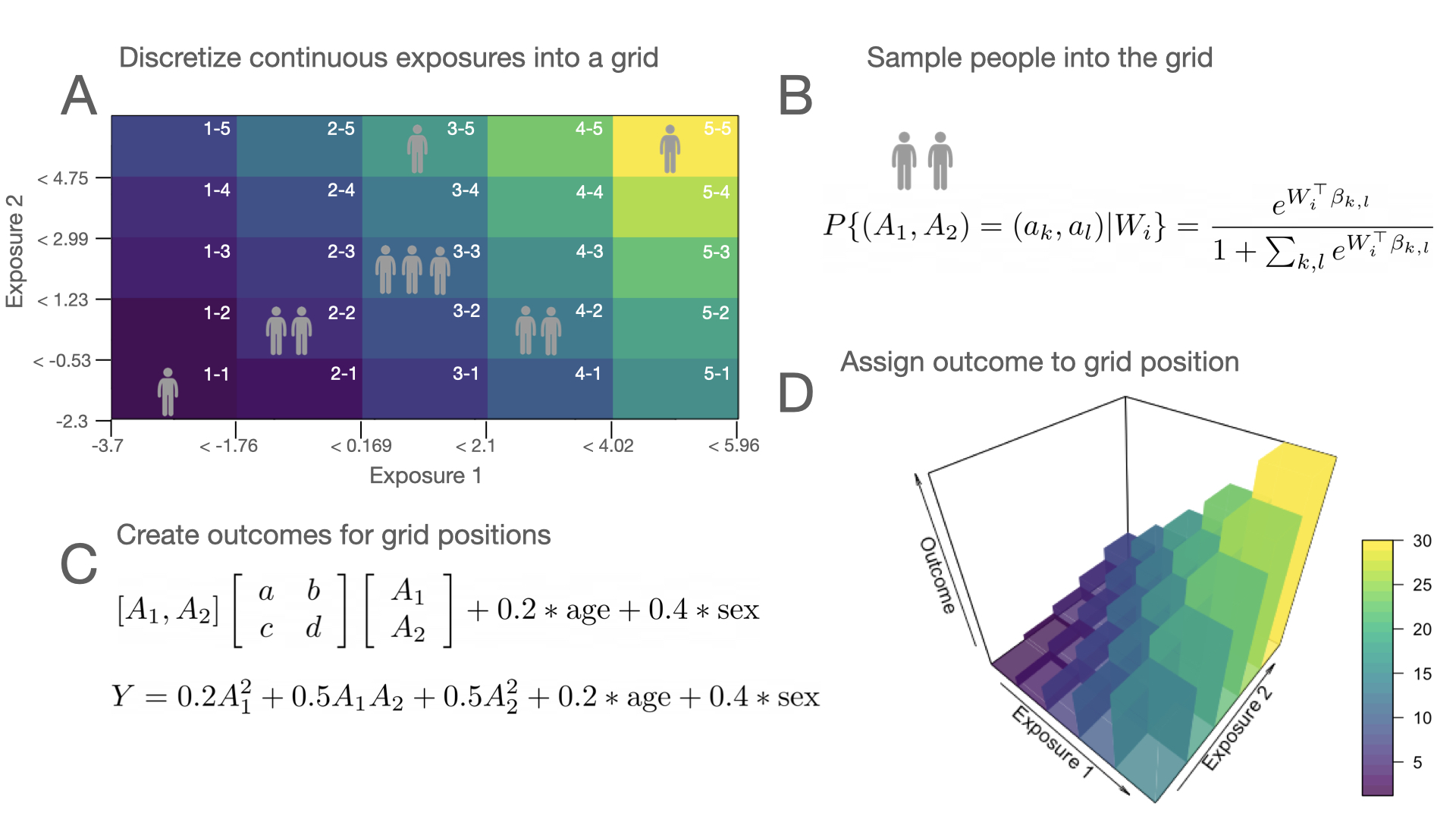
Figure 1: 2D Exposure Simulation

Of course, it is also possible to explore other dose-response relationships (such as logarithmic) by changing the coefficient matrix.

Computing Ground Truth

The fact that our exposures are discrete in this simulation lets us easily compute the ground-truth ARE for any region $\mathcal{A}$ because we can explicitly compute the conditional mean function $m$

$$m(\mathcal{A}=1,w) =\int_{a\in\mathcal{A}}\mu(a,w)\frac{p_{A|W}(a,w)}{\pi_{\mathcal{A}}(w)}\ da$$

$$=\frac{\sum_{a\in\mathcal{A}}\mu(a,w)p_{A|W}(a,w)}{\sum_{a\in\mathcal{A}}p_{A|W}(a)}$$

Therefore to approximate the ARE to arbitrary precision we can

1. Sample a large number of times (e.g. $b=100,000$) from the covariate distribution to obtain $W_{\{1,\dots i,\dots b\}}$.

2. Compute the values $m(\mathcal{A}=1,W_{i})$ using the above formula. This is possible because the functions $\mu$ and $p{A|W}$ are known for the data-generating process . In a similar fashion compute $m(\mathcal{A}=0,w)$.

3. Compute $\text{ARE}(\mathcal{A})=\frac{1}{b}\sum_{i}^{b}m(1,W_{i})-m(0,W_{i})$.

6.1.2 Three-Dimensional Exposure Simulations

This DGS has the same general structure, $O=W,A,Y$. $W$ and baseline covariates

$$W_{1}=\mathcal{N}(\mu=37,\sigma=3),W_{2}=\mathcal{N}(\mu=20,\sigma=1),W_{3}=\mathcal{B}(\mu=0.5)$$

In this 3D simulation we are interested in keeping the exposures continuous as this is more realistic compared to the 2D simulation.

Here $A$ are three continuous mixtures from a multivariate normal distribution:

$$\begin{pmatrix}A_{1}\\ A_{2}\\ A_{3}\end{pmatrix} \sim N\begin{bmatrix}\begin{pmatrix}0\\ 0\\ 0\\ \end{pmatrix}\!\!,&\begin{pmatrix}1.0&0.5&0.8\\ 0.5&1.0&0.7\\ 0.8&0.7&1.0\end{pmatrix}\end{bmatrix}$$

We assign one partition point value to each exposure which creates 8 possible regions in the $2x2x2$ 3D grid for which we want to assign outcomes. Just as the first simulation we want the number of observations in each of the cells in the "mixture cube" to be affected by covariates. To do this we define a conditional categorical distribution $P\{(A_{1},A_{2},A_{3})=(a_{1},a_{2},a_{3})|W=w\}$ and sample from it.

$$P\{(A_{1},A_{2},A_{3})=(a_{k},a_{l},a_{j})|W_{i}\}=\frac{e^{W_{i}^{\top}\beta_{k,l,j}}}{1+\sum_{k,l,j}e^{W_{i}^{\top}\beta_{k,l,j}}}$$

For each of these categories which defines a region in the exposure space we need to assign exposure values while also preserving the local correlation structure within that region. To do this, we convert the cumulative distribution function of the exposures to a uniform distribution then back transform this uniform distribution to the original exposure distribution with bounds for each exposure region. So for instance, in the region where each exposure is less than each threshold value, we back transform the uniform distribution with the minimum value set as the minimum for each exposure and max as the partition value for each exposure. These values then are attached to the categorical variables generated which represent the mixture region. This then generates continuous exposure values with a correlation structure in each region.

The outcome $Y$ is then generated via a linear regression of the form:

$$Y=\beta_{0}+\beta_{1}\mathbbm{1}(A=1)+\beta_{2}\mathbbm{1}(A=2)+...+\beta_{7}\mathbbm{1}(A=7)+\beta_{W_{1}}W_{1}+\beta_{W_{2}}W_{2}+\epsilon,\epsilon~{}N(0,\sigma)$$

Where the $\beta_{j}$ are chosen so some mixture groups have a high mean, some have a low mean and $\mathbbm{1}$ represent indicators of each of the possible 8 regions. Thus, the outcome in each region of the mixture cube is determined by the $\beta$ assigned to that region. Given this formulation of a DGP it is possible to then generate $Y$ by shifting the drivers or "hot spots" around the mixture space, thereby simulating possible agonist and antagonistic relationships. We could assign something like $\beta_{2}=2$ with all other regions having a $\beta_{\neq 2}=0$. This then would mean the ARE in the true DGP is 2. Likewise we could assign $\beta$’s in each region in which case the truth by our definition is the region with the max ARE. The process for this DGP is shown in Figure 2.

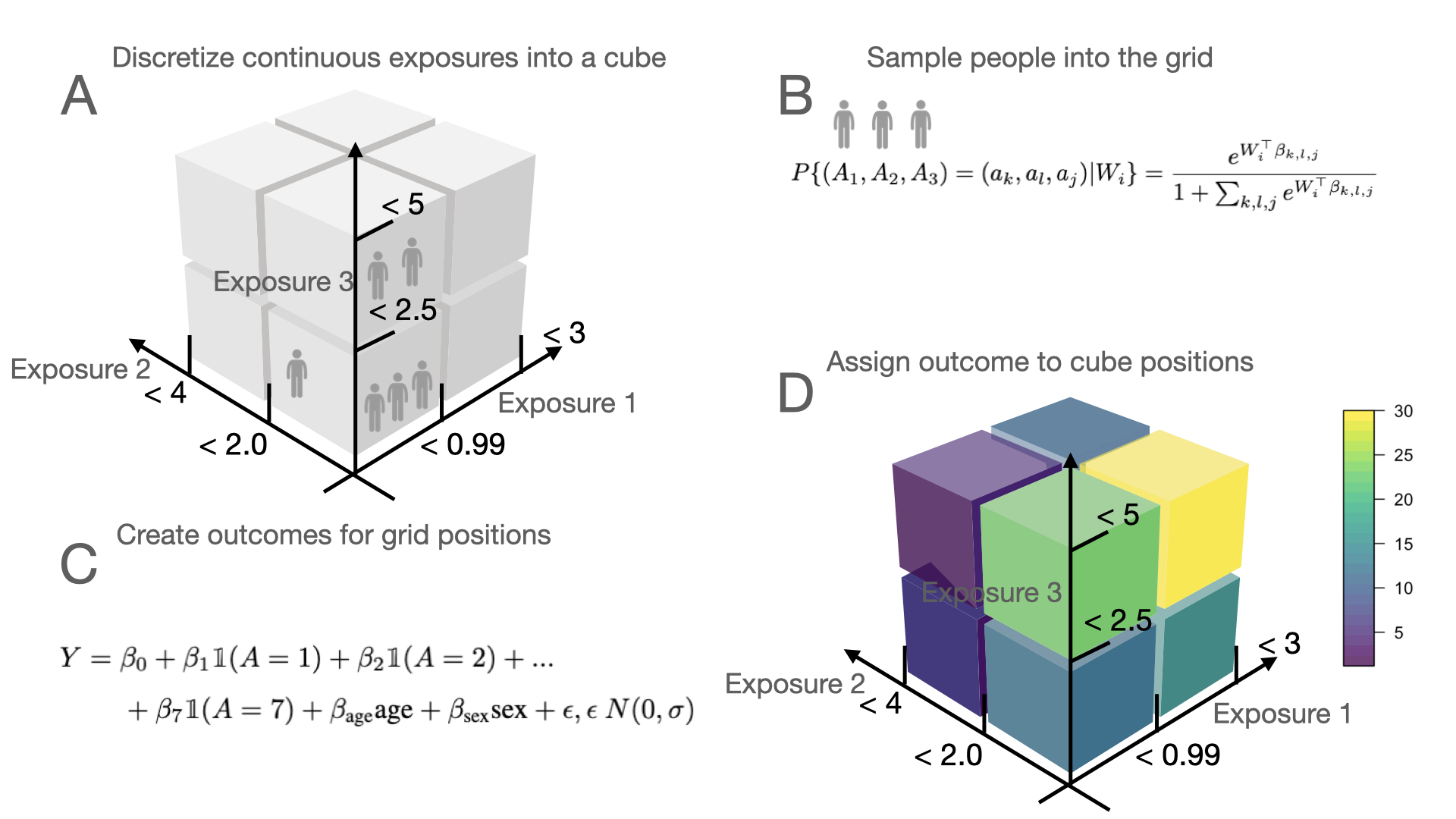
Figure 2: 3D Exposure Simulation

Overall, our 3D example is very similar to the 2D exposure simulation but we aim to test CVtreeMLE in identifying thresholds used to generate an outcome in a space of three continuous exposures. Also, because we keep the space of possible outcomes relatively simple here, we simply generate individual outcomes for each mixture subspace. This allows us to create situations where only one region drives the outcome while the complementary space is 0 or there is an outcome in each region and we are interested in identifying the region with the maximum outcome. In each simulation we are interested in the bias/variance of our estimates compared to the truth, the bias of our rule compared to the true rule and the bias of our data-adaptive rule compared to the expected ARE if that rule was applied to the true population. We discuss this next.

Computing Ground Truth

Previously, in the discrete exposure case, we could directly estimate ground truth by inverse weighting given the summed probability in the exposure region multiplied by the outcome. This is not possible in the continuous case. To make things simpler, we z-score standardize the covariates so the mean of each covariate is 0. Therefore we can directly compute the mean in the region indicated by the ground-truth rule and the mean outcome in the complementary space and take the difference. This is the same as the max coefficient minus the mean of the other coefficients in the linear model, this is the true ARE.

6.2 Evaluating Performance

The following steps breakdown how each simulation was tested to determine 1. asymptotic convergence to the true mixture region used in the DGP, 2. convergence to the true ARE based on this true region and 3. convergence to the true data-adaptive ARE, that is CVtreeMLE’s ability to correctly estimate the ARE if the data-determined rule was applied to the population. We do this by:

1. To approximate $P_{0}$, we draw a very large sample (500,000) from the above described DGP.

2. We then generate a random sample from this DGP of size $n$ which is broken into $K$ equal size estimation samples of size $n_{k}=n/K$ with corresponding parameter generating samples of size $n-n/K$.

3. At each iteration the parameter generating fold defines the region and is used to create the necessary estimators. The estimation fold is used to get our TMLE updated causal parameter estimate, we then do this for all folds.

4. For an iteration, we output the ARE estimates given pooled TMLE, k-fold specific TMLE and the harmonic mean. The region identified in the fold is applied to the large sample $P_{0}$ to estimate the data-adaptive bias. Likewise, each estimate is compared to the ground-truth ARE and region.

For each iteration we calculate metrics for bias, variance, MSE, CI coverage, and confusion table metrics for the true maximal region compared to the estimated region. For each type of estimate (pooled TMLE, k-fold specific TMLE estimates, and harmonic mean) we have bias when comparing our estimate to 1. the ARE based on the true region in the DGP that maximizes the mean difference and 2. the ARE when the data-adaptively determined region is applied to the population. Therefore, when comparing to the true "oracle" region ARE we have:

1. $\psi^{0}_{\text{pooled tmle bias}}$: This is the bias of the pooled TMLE ARE compared to the ground-truth ARE for the true region built into the DGP which maximizes the mean difference in adjusted outcomes.

2. $\psi^{0}_{\text{mean v-fold tmle bias}}$: This is the bias of the mean k-fold specific AREs compared to the ground-truth ARE for the true region built into the DGP.

3. $\psi^{0}_{\text{harmonic mean v-fold tmle bias}}$ This is the bias of the harmonic mean of k-fold specific AREs compared to the ground-truth ARE for the true region built into the DGP.

The above bias metrics are each compared to the true ARE for the oracle region in the DGP. We are also interested in the ARE if the data-adaptively determined region, the region estimated to maximizes the difference in outcomes in the sample data, were applied to $P_{0}$ the true population. Therefore, there are also bias estimates for:

1. $\psi^{DA}_{\text{pooled tmle bias}}$: This is the bias of the pooled TMLE ARE compared to the ARE of the union region across the folds applied to $P_{0}$.

2. $\psi^{DA}_{\text{mean v-fold tmle bias}}$: This is the bias of the mean k-fold specific AREs compared to the mean ARE when all the k-fold specific rules are applied to $P_{0}$.

3. $\psi^{DA}_{\text{harmonic mean k-fold tmle bias}}$ This is the bias of the harmonic mean of k-fold specific AREs compared to the ARE of the union region across the folds applied to $P_{0}$.

We multiple each bias estimate by $\sqrt{n}$ to ensure the rate of convergence is at or faster than $\sqrt{n}$. For each ARE estimate we calculate the variance and subsequently the mean-square error as: $\text{MSE}=\text{bias}^{2}+\text{variance}$. MSE estimates were also multiplied by $n$. For each ARE estimate we calculate the confidence interval coverage of the true ARE parameter givent the oracle region and the ARE given the data-adaptively determined region applied to $P_{0}$. For the TMLE pooled estimates these are lower and upper confidence intervals based on the pooled influence curve. For the k-fold specific coverage, we take the mean lower and upper bounds. For the harmonic pooled coverage, we calculate confidence intervals from the pooled standard error. In each case, we check to see if the ground-truth rule ATE and data-adaptive rule ATE are within the interval. Lastly, we compare the data-adaptively identified region to the ground-truth region using the confusion table metrics for true positive, true negative, false positive and false negative to determine whether, as sample size increases, we converge to the true region.

These performance metrics were calculated at each iteration, where 50 iterations were done for each sample size $n=$ (200, 350, 500, 750, 1000, 1500, 2000, 3000, 5000). It was ensured that, for each data sample, at least one observation existed in the ground-truth region to ensure confusion table estimates could be calculated. CVtreeMLE was run with 5 fold CV (to speed up calculations in the simulations) with default learner stacks for each nuisance parameter and data-adaptive parameter. Our data-adaptive parameter for interactions was the tree with the max ARE (positive coefficient) for each variable set in the ensemble.

6.3 Default Estimators

As discussed, CVtreeMLE needs estimators for $\bar{Q}=E(Y|A,W)$ and $g_{n}=P(A|W)$. CVtreeMLE has built in default algorithms to be used in a Super Learner van der Laan Mark et al. (2007) that are fast and flexible. These include random forest, general linear models, elastic net, and xgboost. These are used to create Super Learners for both $\bar{Q}$ and $g_{n}$. CVtreeMLE also comes with a default tree ensemble which is fit to the exposures during the iterative backfitting procedure. These trees are built from the partykit package Hothorn and Zeileis (2015) in R. By default we include 7 trees in the tree Super Learner that have various levels for the hyper-parameters alpha (p-value to partition on), max-depth (maximum depth of the tree), bonferroni correction (whether to adjust alpha by bonferroni) and min-size (minimum number of observations in terminal leaves). These trees are used during the iterative backfitting in estimating partitions for each individual exposure. For the rule ensemble, the predictive rule ensemble package (pre) Fokkema (2020b) is used with default settings and 10-fold cross-validation. Users can pass in their own libraries for these nuisance and data-adaptive parameters. For these simulations, we use these default estimators in each Super Learner.

6.4 Results

6.4.1 CVtreeMLE Algorithm Identifies the True Region with Maximum ARE

First we describe results for identifying the true region built into the DGP. It is obviously necessary for this to converge to the truth as sample size increases in order for the $\psi^{0}$ estimates to be asymptotically unbiased. Overall we find the tree algorithm identifies the true region in the DGP and therefore provides results which have high-value for treatment policies. Figure 3 shows metrics comparing observations covered by the estimated pooled region to those indicated by the true region in the DGP for two discrete exposures. From this figure it can be seen that, at around 1500 observations, the pooled region is the true region. Figure 4 shows the confusion table metrics comparing the data-adaptive pooled region to the oracle region in the three continuous exposure scenario. As sample size increases, the false positives approach 0 which is what we would desire in this continuous case. From this, we see that in both instances of discrete and continuous exposures, CVtreeMLE is able to identify the correct region in the exposure data which has the maximum ARE. There is some small disparity in the discovered region compared to the truth in the continuous case, this is because for false-positives to perfectly match the true region, the tree search algorithm must identify the exact set of continuous digits that delineate the region which is very difficult. In our case, this region is is $M_{3}$ <= 2.5 & $M_{1}$ >= 0.99 & $M_{2}$ >= 2.0. In this three exposure case there is antagonism of $M_{3}$. Given the exposures are continuous, it is likely that the tree search algorithm gets very close but not absolutely exact to these boundaries. In the two exposure case where the exposures were discretized finding the boundaries is easier. As such, our future evaluation is focused more on the data-adaptive estimates (comparing estimates to the ARE given applying the data-adaptive rule to $P_{0}$). Ultimately, the data-adaptive target parameter theory only holds for the data-adaptive parameter and not the parameter given an oracle rule; however, we include both again to investigate how CVtreeMLE approaches the oracle rule as sample size increases.

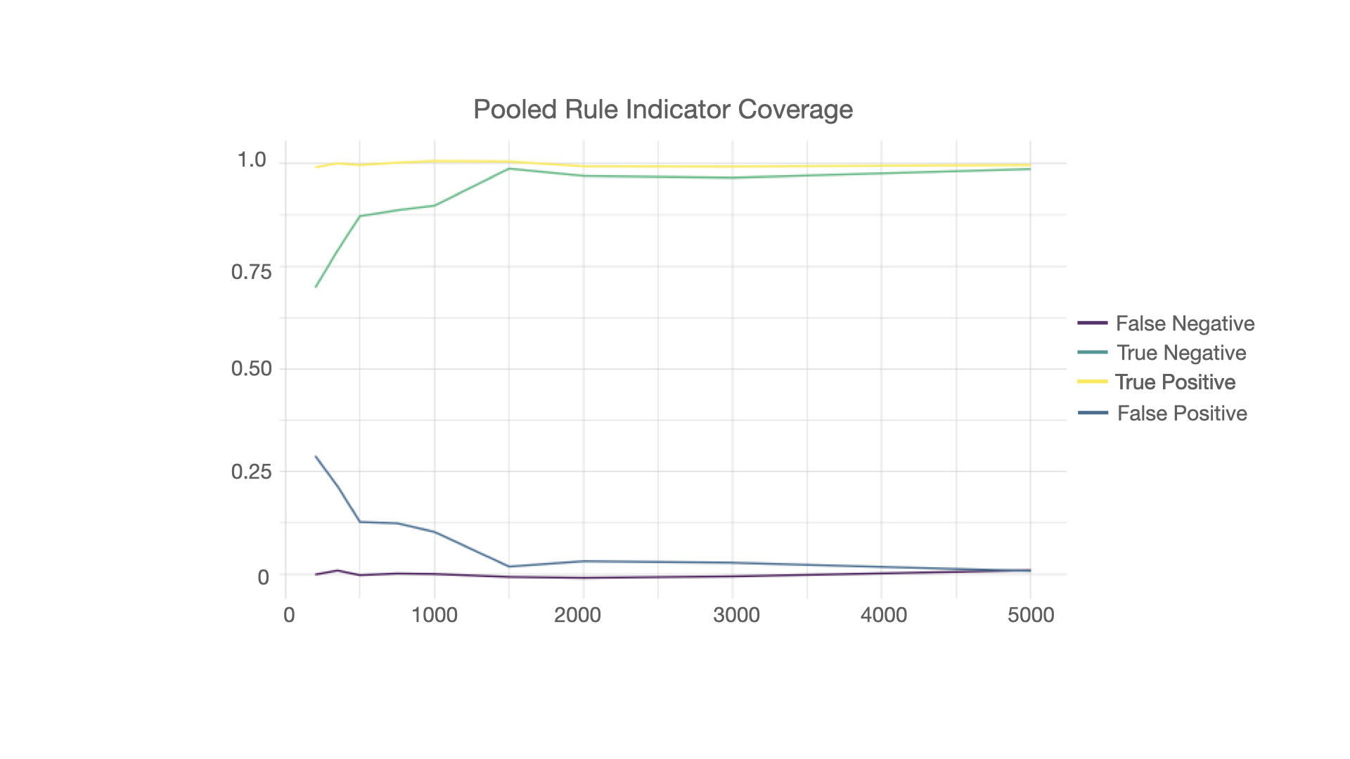
Figure 3: 2D Exposure Confusion Table Metrics of Rule Coverage

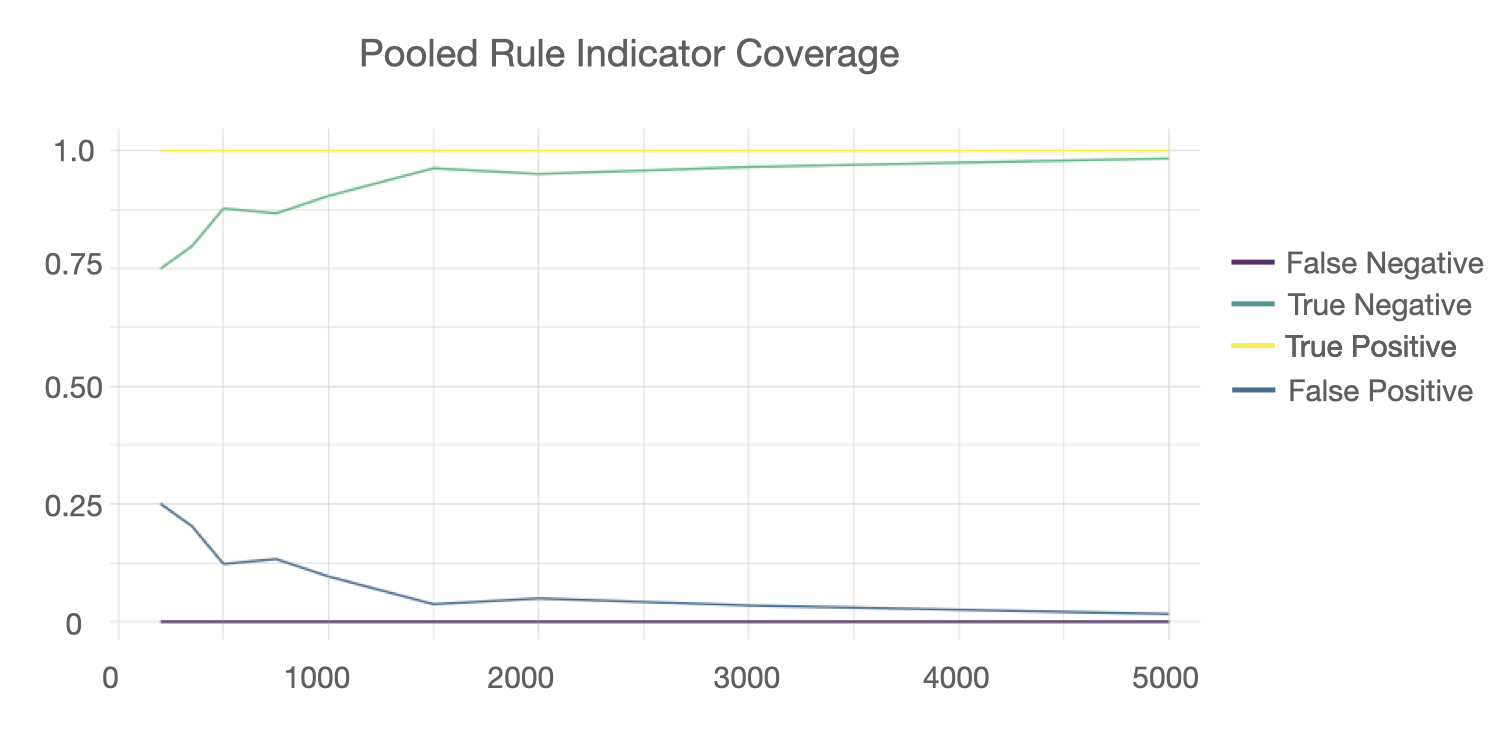
Figure 4: Three Exposure Confusion Table Metrics of Rule Coverage

6.4.2 CVtreeMLE Unbiasedly Estimates the Data-Adaptive Parameter

Looking at the bias for the ARE estimate given two discrete exposures compared to the data-adaptively discovered region applied to $P_{0}$ TMLE unbiasedly estimates the data-adaptive parameter at root $n$ rates with good coverage. Below, Figure 5 A shows the data-adaptive rule ARE bias ($\psi^{DA}_{\text{pooled tmle bias}}$, $\psi^{DA}_{\text{mean k-fold tmle bias}}$, $\psi^{DA}_{\text{harmonic mean k-fold tmle bias}}$) and MSE (B).

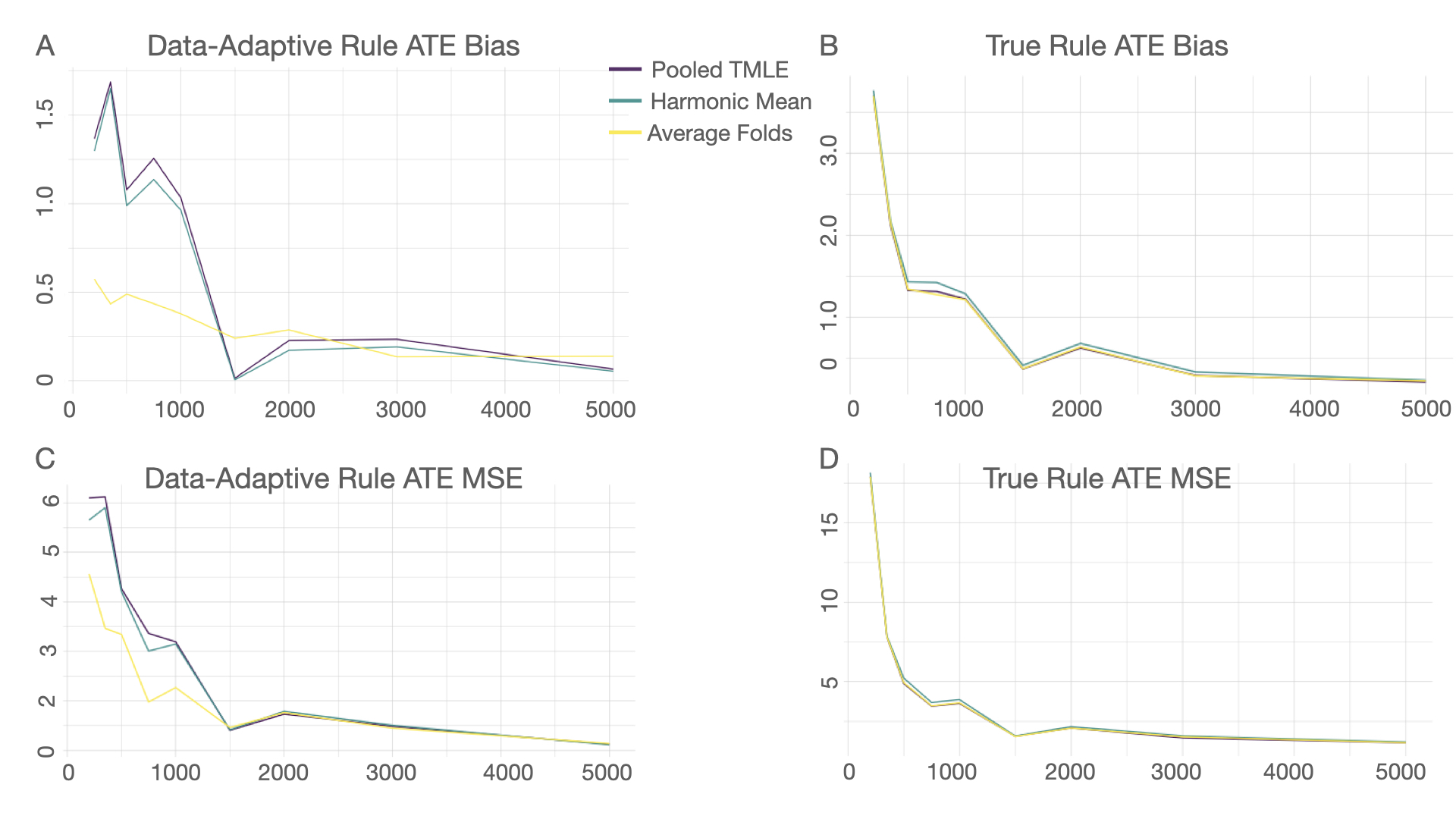
Figure 5: 2D Exposure Bias and MSE

In Figure 5 A the data-adaptive rule ARE bias is larger for the pooled estimates (pooled TMLE ARE and harmonic mean ARE compared to ARE if the pooled rule was applied to $P_{0}$) compared to the average folds bias (mean k-fold ARE compared to the mean of each k-fold rule applied to $P_{0}$). This is because inconsistent rule estimates in lower sample sizes can bias the pooled ARE compared to the pooled region. Consider a 3-fold situation where for variables $X_{1}$ and $X_{2}$ the region was designated by $X_{1}>4\text{ \& }X_{2}>4$, $X_{1}>4\text{ \& }X_{2}>4$, and $X_{1}>2\text{ \& }X_{2}>4$; because $X_{1}>2\text{ \& }X_{2}>4$ is found in one of the folds, this is the pooled region (as it covers observations for $X_{1}>4$) and thus (if the true ARE for $X_{1}>4\text{ \& }X_{2}>4$ applied to $P_{0}$) is higher, our pooled results would be biased to this higher ARE because two of three of our folds have an ARE for this region. This bias converges to average k-fold bias at a sample size of 1500. Effectively, once the trees across the folds stabilizes there is less bias in the pooled estimate compared to the pooled region ATE. This similar pattern is reflected in the pooled estimates MSE (given higher bias in smaller samples). For the user, this indicates that, in smaller sample sizes ($n$ < 1000) the analyst should look at fold specific results to ensure the trees are close in the cut-off values in order to interpret the pooled result. If not, k-fold specific results should be reported as these show very low bias/MSE even in smaller sample sizes. The bias and MSE for all estimates compared to the ground-truth rule ATE show an $1/sqrt(n)$ reduction as sample size increases. In sum, as sample size increases the bias for all estimates converge to 0 which which is necessary for our estimator to have valid confidence intervals.

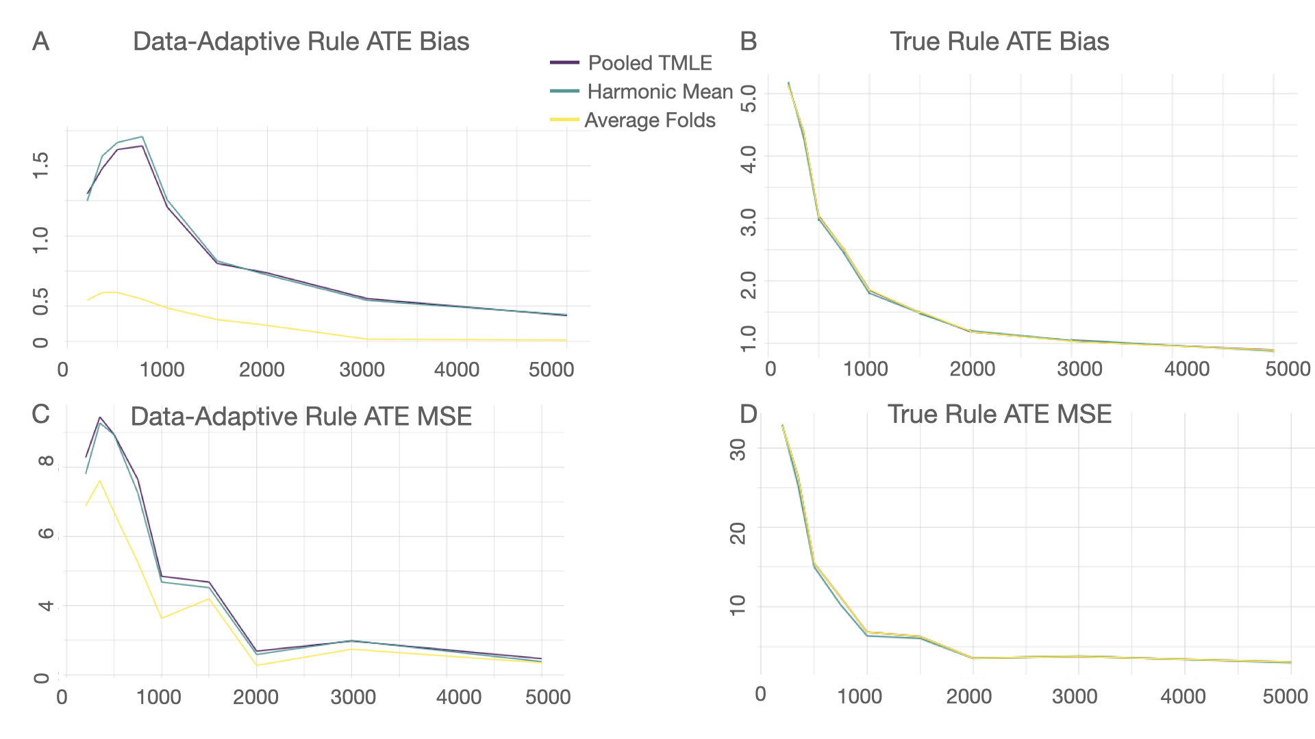
Figure 6: 3D Exposure Bias and MSE

Figure 6 A and C likewise show the asymptotic bias in the three continuous exposure case. All estimates show bias decreasing when evaluated against the ARE when the data-adaptively determined region is applied to $P_{0}$; however, these estimates do not go to 0 exactly (at max sample size equal to 5000) as the data-adaptive rule is still not exactly the true rule, which is expected. Figure 7 A shows the confidence interval coverage for each estimate compared to the data-adaptive region applied to $P_{0}$.

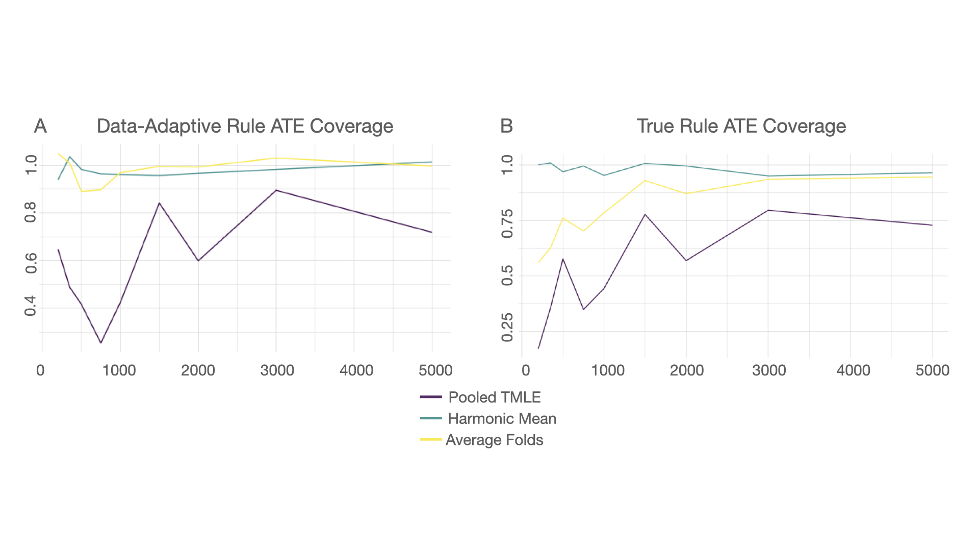
Figure 7: 2D Exposure Confidence Interval Coverage

For coverage of the ARE of the pooled rule applied to $P_{0}$, the CIs calculated from the pooled k-fold standard errors showed coverage between 95% - 100%. The pooled TMLE CIs showed poorer coverage at lower sample sizes, this is likely due to the bias of the pooled ARE estimate compared to the pooled region applied to $P_{0}$ paired with the more narrow confidence intervals calculated across the full sample. The harmonic pooled k-fold CIs were wider and thus covered the truth in this pooled setting. Coverage for the k-fold specific CIs were almost always at or above 90% and converge to 95% at higher sample sizes.

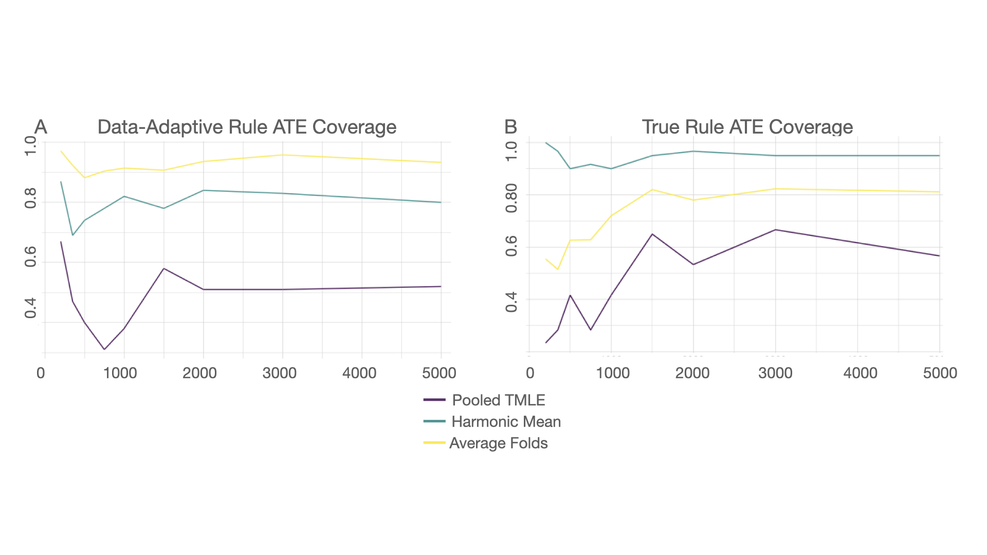
Figure 8: 3D Exposure CI Coverage

Figure 8 A shows the CI coverage of the data-adaptive rule in the three exposures simulation. As expected, the average k-fold CI converges to 95%. The pooled estimates are lower given the conservative pooled rule.

6.4.3 CVtreeMLE Unbiasedly Estimates the Oracle Target Parameter

Now we look at comparing estimates to the true ARE given the oracle region in the DGP. Figure 5 B and D show the bias and MSE for this comparison in the two discrete exposures. As can be seen, both decrease at root $n$ rate for all estimates. Figure 6 B and D likewise show this same rate of convergence for the three continuous exposure case. Based on these simulations, CVtreeMLE unbiasedly estimates the oracle target parameter at root $n$ rates. We next look at the coverage. Figure 7 B shows coverage of the true ARE given the true region. The CIs calculated from the harmonic pooled k-fold standard errors had consistent 95% coverage, the k-fold specific CIs converged to 95% when sample sizes reached 1500 and the pooled TMLE CIs converged to 75% coverage. The same is shown for the three continuous exposures in Figure 8 B the inverse variance CI converges to 95% for coverage of the true ATE with the mean k-fold slightly lower around 82%. Table 2 gives the bias, SD, MSE, and coverage for sample sizes 200, 1000, and 5000, comparing estimates to the data-adaptive truth.

6.4.4 CVtreeMLE has a Normal Sampling Distribution for Valid Inference

For our estimator to have valid inference, we must ensure that the estimator has a normal sampling distribution centered at 0 that gets more narrow as sample size increases. To confirm this, we next examine the empirical distribution of the standardized differences, ($\psi_{n}$ - $\psi^{0}$)/SE($\psi_{n}$), this is the ARE estimate bias compared to the true ARE given the true region divided by the standard error of the estimates over the iterations and $\psi_{n}$ - $\psi^{DA}$)/SE($\psi_{n}$) which is the same standardized difference but compared to the resulting ARE when the data-adaptive region is applied to $P_{0}$. Figure 9 shows the sampling distribution for each sample size with 50 iterations per sample size to estimate the probability density distribution of the standardized bias compared to the data-adaptive ARE. We see convergence to a mean 0 normal sampling distribution as sample size increases for all estimates. Figure 9 A shows the sampling distribution of the standardized bias of the mean k-fold AREs compared to the ground-truth ARE. We can see that this sampling distribution is quite tight around 0. Figures 9 B and C show the sampling distribution for the harmonic mean and the pooled TMLE estimates which are mirror reflections of each other. For both estimates, lower sample sizes (such as in purple $n$ = 200) there is a wider spread of bias (estimates vary more widely) with z-scores out to 2 or 4 but this distribution gets tighter as sample size increases.

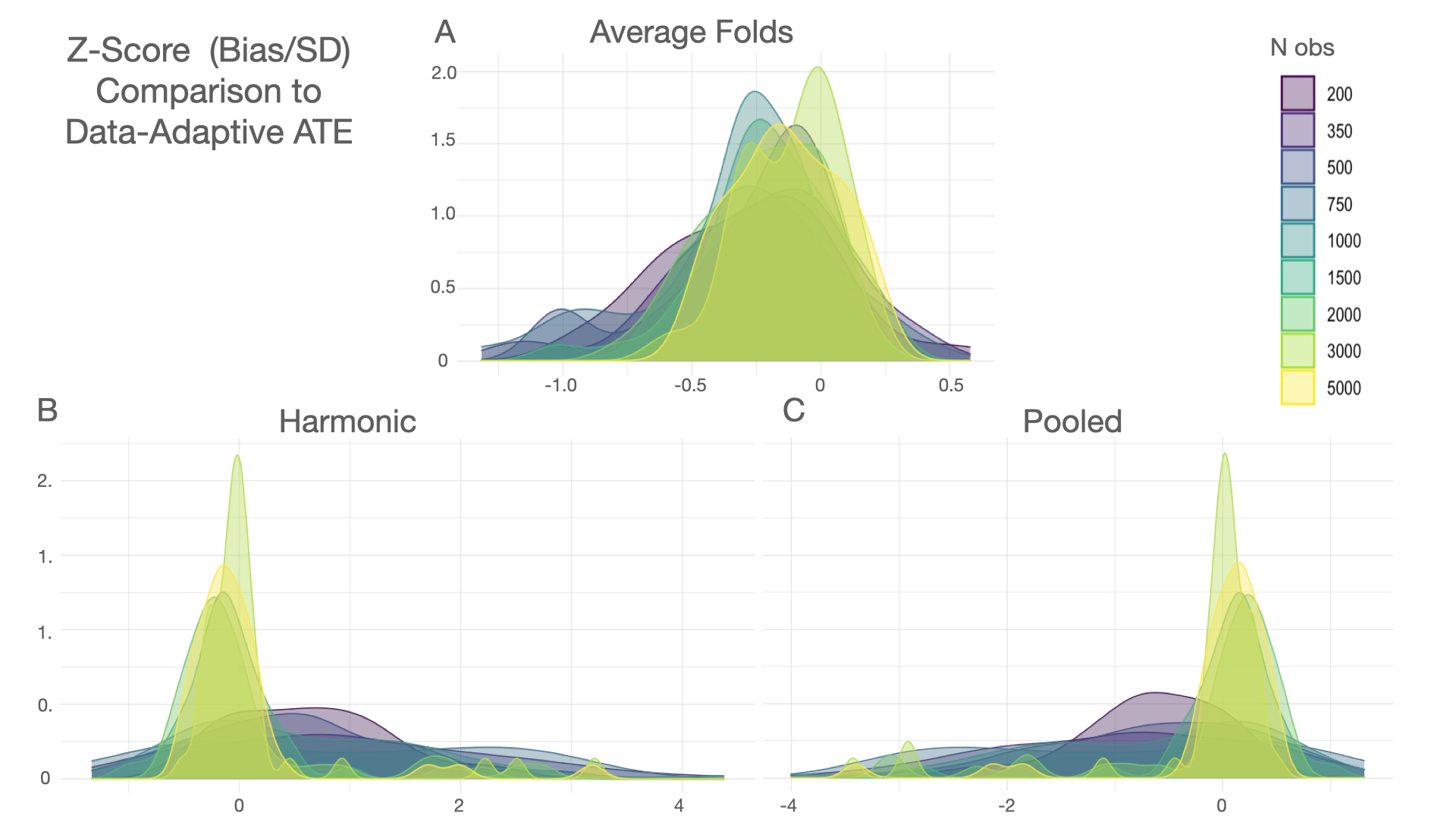
Figure 9: Bias Standardized by Standard Error Compared to ATE of Data-Adaptive Rule

Likewise, Figure 10 A-C show the standardized bias of each estimate compared to the ground-truth region ARE. All estimates generally follow the same distribution and converge to a 0 mean normal distribution as sample size increases.

N	Absolute Bias	SD	MSE	Coverage
200	0.574	2.058	4.565	1
1000	0.379	1.458	2.268	0.97
5000	0.140	1.058	1.138	0.97

Table 1: Simulation results for Estimating the Data-Adaptive ARE using the Average k-fold Estimates

Table 1 shows the results of the simulations based on comparing the mean fold estimated ARE to the mean ARE of data-adaptive rules applied to $P_{0}$. It can be seen that the estimation is unbiased, and the coverage of confidence intervals based IC-based estimates of the standard errors is slightly high. Figure 11 shows the sampling distribution for each sample size for each type of estimate in the three continuous exposures. We see each estimate converge to a mean 0 normal sampling distribution as sample size increases with the average k-fold estimate having a tighter distribution.

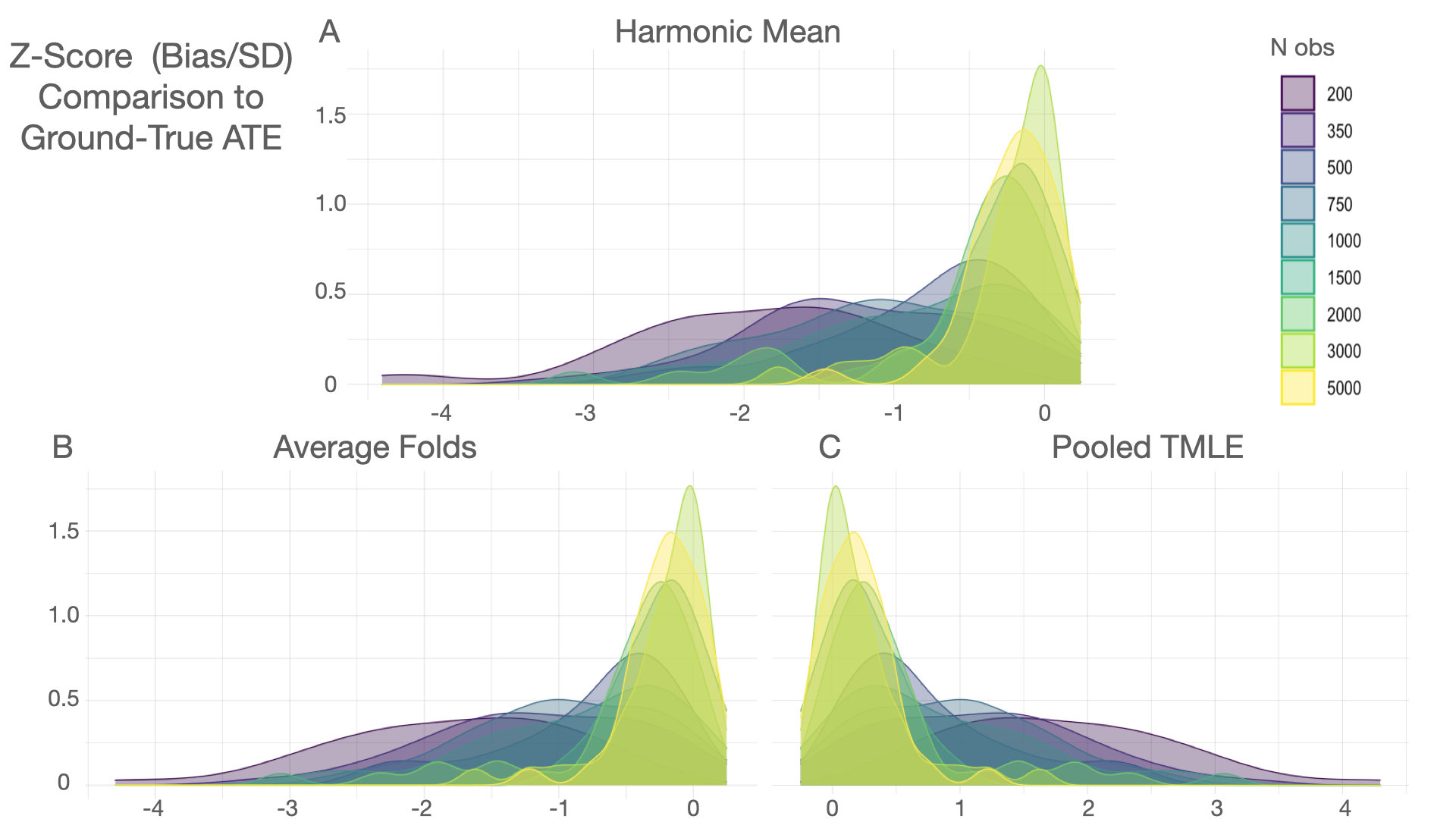
Figure 10: Bias Standardized by Standard Error Compared to ATE of True Rule

N	Absolute Bias	SD	MSE	Coverage
200	0.608	2.10	4.797	0.95
1000	0.382	1.437	2.210	0.95
5000	0.178	0.894	0.831	0.96

Table 2: Simulation results for Estimating the Data-Adaptive ARE using the Average k-fold Estimates in Three Exposure Simulations

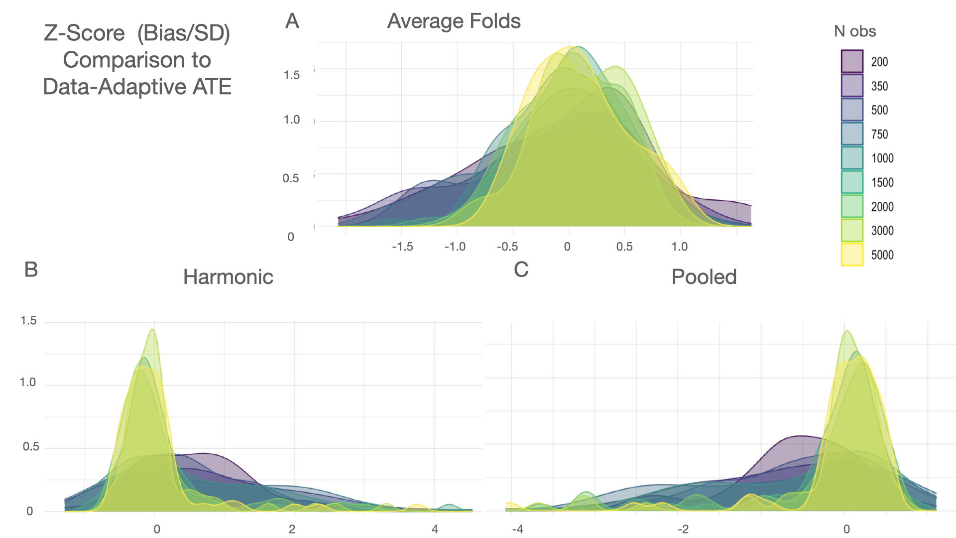
Figure 11: Bias Standardized by Standard Error Compared to ARE of Data-Adaptive Rule for Three Exposures

7 Applications

7.1 NIEHS Synthetic Mixtures

The NIEHS synthetic mixtures data (found here on github) is a commonly used data set to evaluated the performance of statistical methods for mixtures. This synthetic data can be considered the results of a prospective cohort study. The outcome cannot cause the exposures (as might occur in a cross-sectional study). Correlations between exposure variables can be thought of as caused by common sources or modes of exposure. The nuisance variable Z can be assumed to be a potential confounder and not a collider. There are 7 exposures ($X_{1}-X_{7}$) which have a complicated dependency structure with a biologically-based dose response function based on endocrine disruption. For details the github page synthetic data key for data set 1 (used here) gives a description as to how the data was generated. Largely, there are two exposure clusters ($X_{1},X_{2},X_{3}$ and $X_{5},X_{6}$). And therefore, correlations within these clusters are high. $X_{1},X_{2},X_{7}$ contribute positively to the outcome; $X_{4},X_{5}$ contribute negatively; $X_{3}$ and $X_{6}$ do not have an impact on the outcome which makes rejecting these variables difficult given their correlations with cluster group members. This correlation and effects structure is biologically plausible as different congeners of a group of compounds (e.g., PCBs) may be highly correlated, but have different biological effects. There are various agonistic and antagonistic interactions that exist in the exposures. Table 3 gives a breakdown of the variable sets and their relationships.

Variables	Interaction Type
X1 and X2	Toxic equivalency factor, a special case of concentration addition (both increase Y)
X1 and X4	Competitive antagonism (similarly for X2 and X4)
X1 and X5	Competitive antagonism (similarly for X2 and X4)
X1 and X7	Supra-additive (“synergy”) (similarly for X2 and X7)
X4 and X5	Toxic equivalency factor, a type of concentration addition (both decrease y)
X4 and X7	Antagonism (unusual kind) (similarly for X5 and X7)

Table 3: NIEHS Synthetic Data Interactions

Given these toxicological interactions we can expect certain statistical interactions determined as cut-points for sets of variables from CVtreeMLE. For example, we might expect a positive ARE attached to a rule for $X_{1}>=x_{1}\text{ \& }X_{2}>=x_{2}$ where $x_{1},x_{2}$ are certain values for the respective exposures because these two exposures both have a positive impact on Y. Likewise, in the case for antagonistic relationships such as in the case of $X_{2},X_{4}$, we would expect a positive ARE attached to a rule $X_{2}>=x_{2}\text{ \& }X_{4}<=x_{4}$. This is because we might expect the outcome to be highest in a region where $X_{2}$ is high and $X_{4}$ is low given the antagonistic interaction.

The NIEHS data set has 500 observations and 9 variables. Z is a binary confounder. Of course, in this data there is no ground-truth, like in the above simulations, but we can gauge CVtreeMLE’s performance by determining if the correct variable sets are used in the interactions and if the correct variables are rejected. Because many machine learning algorithms will fail when fit with one predictor (in our case this happens for g(Z)), we simulate additional covariates that have no effects on the exposures or outcome but prevent these algorithms from breaking.

We apply CVtreeMLE to this NIEHS synthetic data using 10-fold CV and the default stacks of estimators used in the Super Learner for all parameters. We select for trees with positive coefficients in the ensemble during the data-adaptive estimation and therefore report results as positive AREs. We parallelize over the cross-validation to test computational run-time on a newer personal machine an analyst might be using.

Mixture ATE	Standard Error	Lower CI	Upper CI	P-value	P-value Adj	Vars	Union_Rule
8.24	0.56	7.14	9.34	0.00	0.00	X1-X5	X1 $>$= 0.267 & X5 $<$= 3.189
8.16	0.56	7.07	9.26	0.00	0.00	X1-X7	X1 $>$= 0.326 & X7 $>$= 0.22
6.68	0.62	5.46	7.89	0.00	0.00	X2-X5	X2 $>$= 0.602 & X5 $<$= 3.189
6.82	0.58	5.68	7.95	0.00	0.00	X2-X7	X2 $>$= 0.619 & X7 $>$= 1.171
7.29	0.51	6.29	8.29	0.00	0.00	X5-X7	X5 $<$= 3.269 & X7 $>$= 0.138

Table 4: NIEHS Synthetic Data Consistent Interaction Results

Table 4 shows the results from CVtreeMLE when applied to this NIEHS synthetic data set using the aforementioned settings. We filter results to only interactions that were found in all 10-folds, that is, trees with variable sets found across all the folds and therefore have consistent "signal" in the data. Let’s focus on the second row with variables $X_{1}$ and $X_{7}$. Table 3 shows that these two variables have a supra-additive or synergistic non-additive relationship. The union rule for trees including these two variables was $X1>=0.326\text{ \& }X7>=0.22$ meaning this rule covers all observations indicated by the fold-specific rules. The mixture ARE is then interpreted as, if all individuals were exposed to $X_{1}$ at levels at or greater than 0.326 and exposed to levels of $X_{7}$ at or greater than 0.22 the outcome would be 8.16 units greater compared to if all individuals were exposed to levels less than these respective levels. The subsequent standard errors derived from the pooled influence curve (column 2) are used to derive the confidence intervals and p-values for hypothesis testing. Overall, comparing these statistical interactions to the toxicological interactions listed CVtreeMLE identifies 5 of 9 interactions. The other interactions in the above table are interpreted in the same way as the $X_{1}$ and $X_{7}$ interaction.

We next can investigate how consistent the results are across the folds by looking at the k-fold specific results, this gives us a sense of how reliable our ARE estimates are for the pooled rule. Let’s dig deeper into this $X_{1}$ and $X_{7}$ interaction. Table 5 shows the k-fold specific results for the interactions found for the variables $X_{1}$ and $X_{7}$. Each row is the results for each fold and the final row is the inverse variance weighted pooled result, pooling estimates across the folds. Estimates show stability across the folds with only one fold, fold 8, deviating from the trend. Cut-points at $X_{1}$ were either at 0.991 or 0.998 with fold 8 having a lower cut-point of 0.319. Likewise, $X_{7}$ was partitioned at 0.48 in most folds. Each fold-specific result has valid inference however it is also necessary to evaluate how consistent results were across the folds and thus determine if partitions are stable. Here we see the $X1>=0.99\text{ \& }X7>=0.48$ partition for these two variables is stable and found in 8 of the folds. The ARE estimate for these rules ranges from 8-9 all with a significant effect. CVtreeMLE also provides plots of k-fold estimates to more easily assess for trends, Figure 12 gives an example of this plot for the interaction $X_{1}$ and $X_{7}$.

Mixture ATE	SE	Lower CI	Upper CI	P-Value	P-Value Adj	Mix Rule	Fold
8.09	1.03	6.08	10.10	0.00	0.00	X1 $>$ 0.998 & X7 $>$ 0.48	1
7.12	1.63	3.92	10.32	0.00	0.00	X1 $>$ 0.998 & X7 $>$ 2.108	2
8.38	1.51	5.41	11.34	0.00	0.00	X1 $>$ 0.991 & X7 $>$ 0.48	3
9.42	2.23	5.05	13.80	0.00	0.00	X1 $>$ 0.991 & X7 $>$ 0.441	4
8.81	1.76	5.36	12.26	0.00	0.00	X1 $>$ 0.998 & X7 $>$ 0.439	5
8.43	1.53	5.42	11.43	0.00	0.00	X1 $>$ 1.049 & X7 $>$ 0.482	6
8.84	1.84	5.23	12.44	0.00	0.00	X1 $>$ 0.991 & X7 $>$ 0.413	7
5.20	2.69	-0.07	10.48	0.05	0.53	X7 $>$ 0.217 & X1 $>$ 0.319	8
8.41	1.04	6.36	10.46	0.00	0.00	X1 $>$ 0.991 & X7 $>$ 0.482	9
8.94	1.39	6.22	11.67	0.00	0.00	X1 $>$ 0.991 & X7 $>$ 0.482	10
8.30	5.49	-2.45	19.05	0.13	0.13	X1 $>$= 0.326 & X1 $<$= 4.687 & X7 $>$= 0.22 & X7 $<$= 4.886	Pooled

Table 5: $X_{1}$ and $X_{7}$ k-fold Interaction Results

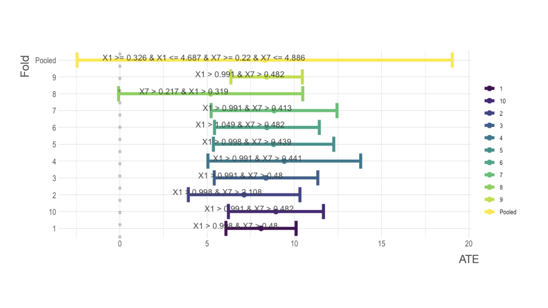
Figure 12: K-fold specific results for the interaction $X_{1}$ and $X_{7}$

Overall, CVtreeMLE is able to determine subspaces in the respective variables that have the most impact on the endocrine disrupting outcome. Of note is the fact that no interactions include the variables $X_{3}$ and $X_{6}$ both of which have no impact on the outcome.

7.1.1 Comparison to Existing Methods

Currently, quantile g-computation is a popular method for mixture analysis in environmental epidemiology. The method yields estimates of the effect of increasing all exposures by one quantile, simultaneously under linear model assumptions. Quantile g-computation looks like:

$$Y_{i}=\beta_{0}+\sum_{j=1}^{d}\beta_{j}X_{ji}^{q}+\beta Z_{i}+\epsilon_{i}$$

Where $X^{q}$ are the quantized mixture components and $Z$ are the covariates. Which works by first transforming mixture components into quantiles. Then the negative and positive coefficients from a linear model for the mixture components are summed to give a mixture ($\Psi$) summary measure which characterizes the joint impact. There are many assumptions that should be poignant after our discussion of mixtures. Firstly, quantiles may not characterize the exposure-response relationship (could be non-monotonic) which occurs in endocrine disrupting compounds. For interpretable weights and mixture estimate $\Psi$, assumes additive relationship of quantiles ($\Psi$ is just sum of $\beta$’s in front of mixture components). After our discussion, in mixtures our main goal is model possible interactions in the data because we expect exposures to have non-additive, possible non-monotonic, antagonistic and agonistic relationships. Therefore, we should expect interactions in our mixture data. In quantile g-computation, with the inclusion of interactions, the proportional contribution of an exposure to the overall effect then varies according to levels of other variables and therefore weights cannot be estimated. Because we can never assume no interactions, quantile g-computation then boils down to getting conditional expectations when setting mixtures to quantiles through a linear model with interaction terms specified by the analyst. After our discussion of mixtures this should feel incorrect. As we argue, the important variables, relationships, and thresholds in a mixture are all unknown to the analyst which makes this a data-adaptive target parameter problem. Even testing quantile g-computation on the NIEHS data is difficult because we don’t know what interactions to include a priori. The best we can do is run it out of the box and with two-way interactions and compare results to the ground-truth measures. Lastly, quantile g-computation does not flexibly control for covariates.

We run quantile g-computation on the NIEHS data using 4 quantiles with no interactions to investigate results using this model. The scaled effect size (positive direction, sum of positive coefficients) was 6.28 and included $X_{1},X_{2},X_{3},X_{7}$ and the scaled effect size (negative direction, sum of negative coefficients) was -3.68 and included $X_{4},X_{5},X_{6}$. Compared to the NIEHS ground-truth, $X_{3},X_{6}$ are incorrectly included in these estimates. However the positive and negative associations for the other variables are correct.

Next, because we expect interactions to exist in the mixture data, we would like to assess for them but the question is which interaction terms to include? Our best guess is to include interaction terms for all the exposures. We do this and show results in Table 6.

	Estimate	Std. Error	Lower CI	Upper CI	Pr($>$$|$t$|$)
(Intercept)	21.29	1.58	18.19	24.39	0.00
psi1	0.02	1.62	-3.16	3.20	0.99
psi2	0.59	0.67	-0.71	1.90	0.37

Table 6: Quantile G-Computation Interaction Results from NIEHS Synthetic Data

In Table 6 $\Psi_{1}$ is the summary measure for main effects and $\Psi_{2}$ for interactions. As can be seen, when including all interactions neither of the estimates are significant. Of course this is to be expected given the number of parameters in the model and sample size $n=500$. However, moving forward with interaction assessment is difficult, if we were to assess for all 2-way interaction of 7 exposures the number of sets is 21 and with 3-way interactions is 35. We’d have to run this many models and then correct for multiple testing. Hopefully this example shows why mixtures are inherently a data-adaptive problem and why popular methods such as this, although succinct and interpretable, fall short even in a simple synthetic data set.

7.2 NHANES Data

Environmental chemical and metal exposure can affect telomere length, which is a mediating pathway for adverse health outcomes including cancer. Studies on the association of metals with leucocyte telomere length (LTL) are mainly limited to single-metal effect Xia et al. (2022); Zota et al. (2015); Clarity et al. (2021). Some research has investigated the overall joint associations metal mixture with LTL using parameteric models like multiple linear regression or quantile-sum g-computation Keil et al. (2019); Lai et al. (2022). Since environmental stressors are known to disrupt telomere length homeostasis which plays a crucial role in cellular aging and disease we investigate the association of mixed metal exposure on LTL. Our desires are two fold, 1. to show CVtreeMLE results applied to real-world data and 2. to provide such data and data processing code with the open-source CVtreeMLE package. As such, we develop a pipeline to download and clean National Health and Nutrition Examination Survey (NHANES) dataset. We download and format the relevant NHANES 1999–2002 dataset containing demographic data, disease history, nine urine metals, and LTL. The demographic data used as possible confounders ($W$) include age, gender, race, education level, marital status, alcohol, smoking (cotinine) , body mass index (BMI), family poverty ratio (PIR), fasting glucose, systolic and diastolic blood pressure, exercise and birth country. Urine metal contained barium (Ba), cadmium (Cd), cobalt (Co), cesium (Cs), molybdenum (Mo), lead (Pb), antimony (Sb), thallium (Tl) and tungsen (W). The outcome is LTL. The number of observations in this test data is 2510. The coding pipeline and data are available in the CVtreeMLE package.

We apply CVtreeMLE using the default learners in each stack. We use 10-fold CV and set the max number of iterations in the iterative backfitting to 10 as well. Because previous research has shown the exposure to metals shortens LTL, we set the ATE direction to negative to select trees in the data-adaptive procedure which have the minimum (negative) impact and thus return negative ATEs for each fold.

Mixture ATE	Standard Error	Lower CI	Upper CI	P-value	P-value Adj	Vars	Union_Rule	%Fold
0.06	0.04	-0.02	0.13	0.17	1.00	cadmium-molybdenum	cadmium $>$= 0 & cadmium $<$= 0.715 & molybdenum $>$= 19.8 & molybdenum $<$= 436.8	0.80
-0.03	0.01	-0.06	-0.01	0.02	0.37	cadmium-thallium	cadmium $>$= 0.027 & cadmium $<$= 36.777 & thallium $>$= 0.01 & thallium $<$= 0.38	1.00

Table 7: Consistent Pooled TMLE Results NHANES Metal Mixture-LTL

Table 7 shows the pooled TMLE ARE results for rules found in more than 75% of the folds. Here we see rules including cadmium and thallium were found in all the folds and rules including cadmium and molybdenum were found in 80% of the folds. The cadmium-thallium interaction had a significant ARE of -0.03 and the cadmium-molybdenum was borderline significant with an ARE of 0.06. These results show that, exposure to high levels of cadmium >= 0.027 and low levels of thallium <= 0.38 is associated with a reduced telomere length of 0.03 compared to exposure levels of cadmium levels lower than 0.027 and thallium levels greater than 0.38. This result implies an antagonistic relationship between cadmium and thallium. Likewise, telomere length was longer (0.06) for those exposed to low levels of cadmium <= 0.715 and high levels of molybdenum >= 19.8 compared to those exposed to the inverse exposure region for these two metals.

Like the NIEHS synthetic data results, we can investigate the k-fold specific results for these pooled results. Let’s look at the cadmium and thallium interaction in each fold to see how stable the partition points were for each metal.

ATE	SE	Lower CI	Upper CI	P-Value	P-Value Adj	Mix Rule
-0.03	0.06	-0.15	0.09	0.67	1.00	thallium $<$= 0.21 & cadmium $>$ 0.243
-0.04	0.03	-0.10	0.03	0.24	1.00	cadmium $>$ 0.295 & thallium $<$= 0.31
-0.03	0.03	-0.09	0.03	0.32	1.00	thallium $<$= 0.21 & cadmium $>$ 0.101
-0.05	0.04	-0.13	0.02	0.14	1.00	cadmium $>$ 0.097 & thallium $<$= 0.38
-0.03	0.03	-0.09	0.03	0.37	1.00	cadmium $>$ 0.295 & thallium $<$= 0.21
-0.03	0.05	-0.12	0.06	0.54	1.00	thallium $<$= 0.21 & cadmium $>$ 0.143
-0.04	0.08	-0.20	0.12	0.62	1.00	cadmium $>$ 0.29 & thallium $<$= 0.21
-0.04	0.05	-0.14	0.06	0.44	1.00	thallium $<$= 0.36 & cadmium $>$ 0.092
-0.02	0.06	-0.13	0.10	0.76	1.00	cadmium $>$ 0.027 & thallium $<$= 0.14
-0.03	0.04	-0.11	0.05	0.52	1.00	thallium $<$= 0.22 & cadmium $>$ 0.254
-0.03	0.16	-0.34	0.27	0.83	0.83	cadmium $>$= 0.027 & thallium $<$= 0.38

Table 8: K-fold specific results for cadmium-thallium interactions associated with LTL

Table 8 shows the k-fold specific results for cadmium and thallium interaction. This interaction was found in all the folds with an ARE ranging from -0.02 to -0.05. None of the fold specific results were significant due to the variance estimates being calculated on the 251 observations in each validation fold, making standard errors high. However, we see consistent partitioning of thallium between 0.14 and 0.38 and partitioning of cadmium between 0.027 and 0.29. Overall, we see consistent cut-points across the folds which indicates this interaction is stable. The last row in this table is the inverse weighted pooled results. Here we can see that we gain much power by using the pooled influence curve in the pooled TMLE procedure which is able to borrow variance information across the folds because all estimates are cross-estimated. Here, we can see the pooled estimated has much higher variance and wider confidence intervals.

ATE	SE	Lower CI	Upper CI	P-Value	P-Value Adj	Mix Rule	fold
0.05	0.04	-0.04	0.14	0.30	1.00	molybdenum $>$ 55.2 & cadmium $<$= 0.384	2
0.04	0.10	-0.15	0.23	0.68	1.00	molybdenum $>$ 52.9 & cadmium $<$= 0.368	3
0.01	0.04	-0.07	0.09	0.77	1.00	cadmium $<$= 0.715 & molybdenum $>$ 19.7	4
0.11	0.14	-0.16	0.37	0.42	1.00	cadmium $<$= 0.35 & molybdenum $>$ 102.5	5
0.05	0.05	-0.04	0.14	0.27	1.00	cadmium $<$= 0.292 & molybdenum $>$ 57.2	6
0.02	0.22	-0.41	0.46	0.92	1.00	cadmium $<$= 0.124 & molybdenum $>$ 21.7	7
0.02	0.06	-0.09	0.14	0.71	1.00	cadmium $<$= 0.429 & molybdenum $>$ 44.5	8
0.14	0.28	-0.42	0.69	0.63	1.00	cadmium $<$= 0.131 & molybdenum $>$ 55.6	9
0.04	0.41	-0.77	0.84	0.93	0.93	cadmium $>$= 0 & cadmium $<$= 0.715 & molybdenum $>$= 19.8 & molybdenum $<$= 436.8	Pooled

Table 9: K-fold specific results for cadmium-molybdenum interactions associated with LTL

Lastly, we look at the cadmium-molybdenum interactions in Table 9 . As we can see here, interactions are not found in every fold and the partition points have a larger range although they all point in the same direction (low cadmium and high molybdenum) and all fold specific results are positive. This makes sense given that molybdenum processes proteins and genetic material like DNA and helps break down drugs and toxic substances that enter the body. Therefore, we would expect low cadmium and high molybdenum to be associated with higher telomere length.

Overall, in this NHANES example, we show that in real world data, CVtreeMLE can answer questions regarding expected outcomes under different exposure levels of a mixture which are otherwise occult given the limitation of existing methods.

8 Software

The development of asymptotically linear estimators for data-adaptive parameters are critical for the field of mixed exposure statistics. However, the development of open-source software which translates semi-parametric statistical theory into well-documented functional software is a formidable challenge. Such implementation requires understanding of causal inference, semi-parametric statistical theory, machine learning, and the intersection of these disciplines. The CVtreeMLE R package provides researchers with an open-source tool for evaluating the causal effects of a mixed exposure using the methodology described here. The CVtreeMLE package is well documented and includes a vignette detailing semi-parametric theory for data-adaptive parameters, examples of output, results with interpretations under various real-life mixture scenarios, and comparison to existing methods. The NIEHS synthetic data and the NHANES mixed metal exposure data are provided. The NIEHS synethetic data application is used in the vignette of the package which makes these results reproducible to any researcher and likewise the NHANES data and code are provided for reproducibility. CVtreeMLE can run sequentially or parallelized across folds using the furrr package Vaughan and Dancho (2022). New statistical software using machine learning often presume the availability of significant computational resources in order to run in a timely manner. Here, our applications of NIEHS and NHANES were all run on a personal macbook machine in under 30 minutes by utilizing parallelization and using flexible yet efficient estimators. Of course, for the simulations high performance computing was used to parallelize iteration over clusters. To-date in scientific publication, the release of reproducible software is the exception rather than the rule. In an effort to make robust statistical software adopted in the future, rather than reliance of simple parameteric models, we make CVtreeMLE available with clear, easily accessible, highly detailed documentation of the coding methods. We also make all functions user-accessible, and develop numerous tests and examples. Coding notebooks show simulations of mixed exposure data and CVtreeMLE output with detailed summaries of interpretation. Lastly, the CVtreeMLE package is well maintained to ensure accessibility with ongoing improvements tested at each iteration. The CVtreeMLE package has been made publicly available via GitHub. The pseduo-code that describes the code which executes the described method is shown in Figure 13.

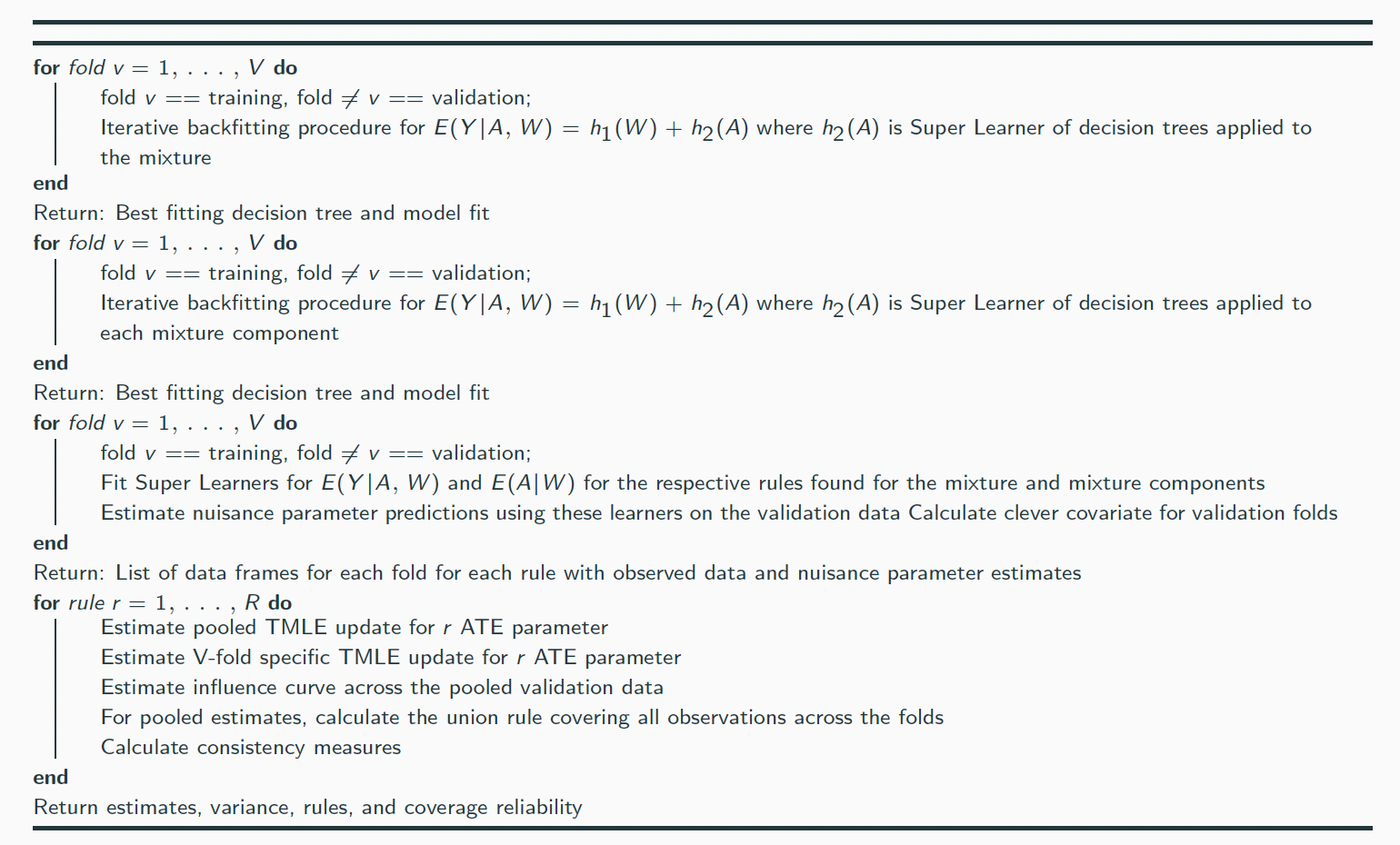
Figure 13: CVtreeMLE Pseudo-Code

9 Discussion

In this paper we introduce a new method for estimating the effects of a mixed exposure. Our approach treats ensemble decision trees as a data-adaptive target parameter for which we estimate the average effects of exposure for regions identified in the best fitting decision trees. This is done within a cross-validated framework paired with targeted learning of our target parameter which provides estimates that are asymptotically unbiased and have the lowest variance for studies which satisfy the unconfoundedness and positivity assumptions. Our proposed method provides valid confidence intervals without restrictions on the number of exposure, covariates, or the complexity of the data-generating process. Our method first partitions the exposure space into subspaces or regions that best explains the outcome. The output of our method is the exposure effect and respective confidence intervals if all individual were exposed to the exposure region compared to if all individual were not exposed to this region. Our approach has potentially many important applications including identifying what combinations of drugs lead to the most beneficial patient outcomes as well as finding what combinations of pollution chemicals have the most deleterious outcomes on public health. Our approach allows for "dredging with dignity" wherein exposure regions can be discovered in the data which are not known a priori and still provide unbiased estimates for the target parameter with valid confidence intervals. This approach of course comes with some cost as construction of a pooled region across the folds is rather ad hoc. This is the main limitation in the proposed method and other alternatives may exist such as using the average partitioning values of each exposure variable rather than our union approach which is conservative. Our simulations with ground-truth, NIEHS synethetic data and real-world data application show the robustness and interpretability of our approach. In an effort to make adoption of semi-parametric methods such as this more seamless we provide the CVtreeMLE R package on github which is well documented for analysts to apply to their respective data.

10 Appendix

References

- Safe [1993] S. Safe. Toxicology, structure-function relationship, and human and environmental health impacts of polychlorinated biphenyls: Progress and problems. Environmental Health Perspectives, 100:259–268, 1993. ISSN 00916765. doi:10.1289/ehp.93100259.
- Kortenkamp [2007] Andreas Kortenkamp. Ten years of mixing cocktails: A review of combination effects of endocrine-disrupting chemicals. Environmental Health Perspectives, 115(SUPPL1):98–105, 2007. ISSN 00916765. doi:10.1289/ehp.9357.
- Keil et al. [2019] Alexander P. Keil, Jessie P. Buckley, Katie M. O’Brien, Kelly K. Ferguson, Shanshan Zhao, and Alexandra J. White. A quantile-based g-computation approach to addressing the effects of exposure mixtures. arXiv, 128(April):1–10, 2019. ISSN 23318422. doi:10.1097/01.ee9.0000606120.58494.9d.
- De Vocht et al. [2012] Frank De Vocht, Nicola Cherry, and Jon Wakefield. A Bayesian mixture modeling approach for assessing the effects of correlated exposures in case-control studies. Journal of Exposure Science and Environmental Epidemiology, 22(4):352–360, 2012. ISSN 15590631. doi:10.1038/jes.2012.22.
- Bobb et al. [2014] Jennifer F. Bobb, Linda Valeri, Birgit Claus Henn, David C. Christiani, Robert O. Wright, Maitreyi Mazumdar, John J. Godleski, and Brent A. Coull. Bayesian kernel machine regression for estimating the health effects of multi-pollutant mixtures. Biostatistics, 16(3):493–508, 2014. ISSN 14684357. doi:10.1093/biostatistics/kxu058.
- National Institute of Environmental Health Sciences (2018) [NIEHS] National Institute of Environmental Health Sciences (NIEHS). 2018-2023 Strategic Plan. National Institutes of Health, 2018. URL https://www.niehs.nih.gov/about/strategicplan/strategicplan20182023_508.pdf.
- Leo Breiman [1984] Charles J. Stone R.A. Olshen Leo Breiman, Jerome Friedman. Classification and Regression Trees. Chapman and Hall/CRC, 1984.
- Athey and Imbens [2016] Susan Athey and Guido Imbens. Recursive partitioning for heterogeneous causal effects. Proceedings of the National Academy of Sciences of the United States of America, 113(27):7353–7360, 2016. ISSN 10916490. doi:10.1073/pnas.1510489113.
- Hubbard et al. [2016] Alan E. Hubbard, Sara Kherad-Pajouh, and Mark J. Van Der Laan. Statistical Inference for Data Adaptive Target Parameters. International Journal of Biostatistics, 12(1):3–19, 2016. ISSN 15574679. doi:10.1515/ijb-2015-0013.
- Zheng and van der Laan [2010] Wenjing Zheng and MJ van der Laan. Asymptotic theory for cross-validated targeted maximum likelihood estimation. U.C. Berkeley Division of Biostatistics Working Paper Series, (273), 2010. URL http://biostats.bepress.com/ucbbiostat/paper273/.
- Hastie and Tibshirani [1990] Trevor Hastie and Robert Tibshirani. Generalized additive models. Wiley Online Library, 1990.
- van der Laan Mark et al. [2007] J. van der Laan Mark, Polley Eric C, and Hubbard Alan E. Super learner. Statistical Applications in Genetics and Molecular Biology, 6(1):1–23, 2007. URL https://EconPapers.repec.org/RePEc:bpj:sagmbi:v:6:y:2007:i:1:n:25.
- Hejazi et al. [2021] Nima S. Hejazi, Mark J. van der Laan, Holly E. Janes, Peter B. Gilbert, and David C. Benkeser. Efficient nonparametric inference on the effects of stochastic interventions under two-phase sampling, with applications to vaccine efficacy trials. Biometrics, 77(4):1241–1253, 2021. ISSN 15410420. doi:10.1111/biom.13375.
- Hejazi et al. [2022] Nima S Hejazi, Kara E Rudolph, Mark J Van Der Laan, and Iván Díaz. Nonparametric causal mediation analysis for stochastic interventional (in)direct effects. Biostatistics, pages 1–22, 2022. ISSN 1465-4644. doi:10.1093/biostatistics/kxac002.
- Iván Díaz Muñoz and Mark van der Laan* [2012] Iván Díaz Muñoz and Mark van der Laan*. Population Intervention Causal Effects Based on Stochastic Interventions. Biometrics., 68(2):541–549, 2012. ISSN 15378276. doi:10.1111/j.1541-0420.2011.01685.x.Population. URL https://www.ncbi.nlm.nih.gov/pmc/articles/PMC3624763/pdf/nihms412728.pdf.
- Nichols [2007] Austin Nichols. Causal inference with observational data. The Stata Journal, 7(4):507–541, 2007. doi:10.1177/1536867X0800700403.
- Winship and Morgan [1999] Christopher Winship and Stephen L. Morgan. The estimation of causal effects from observational data. Annual Review of Sociology, 25(May):659–707, 1999. ISSN 03600572. doi:10.1146/annurev.soc.25.1.659.
- Rubin [2006] Donald B. Rubin. Estimating causal effects from large data sets using propensity scores. Matched Sampling for Causal Effects, pages 443–453, 2006. ISSN 0003-4819. doi:10.1017/CBO9780511810725.035.
- Zivich and Breskin [2021] Paul N. Zivich and Alexander Breskin. Machine Learning for Causal Inference: On the Use of Cross-fit Estimators. Epidemiology, 32(3):393–401, 2021. ISSN 15315487. doi:10.1097/EDE.0000000000001332.
- Luque-Fernandez et al. [2018] Miguel Angel Luque-Fernandez, Michael Schomaker, Bernard Rachet, and Mireille E. Schnitzer. Targeted maximum likelihood estimation for a binary treatment: A tutorial. Statistics in Medicine, 37(16):2530–2546, 2018. ISSN 10970258. doi:10.1002/sim.7628.
- Smith et al. [2022] Matthew J. Smith, Mohammad A. Mansournia, Camille Maringe, Paul N. Zivich, Stephen R. Cole, Clémence Leyrat, Aurélien Belot, Bernard Rachet, and Miguel A. Luque-Fernandez. Introduction to computational causal inference using reproducible Stata, R, and Python code: A tutorial. Statistics in Medicine, 41(2):407–432, 2022. ISSN 10970258. doi:10.1002/sim.9234.
- van der Laan and Rose [2011] M.J. van der Laan and S. Rose. Targeted Learning: Causal Inference for Observational and Experimental Data. Springer Series in Statistics. Springer New York, 2011. ISBN 9781441997821. URL https://books.google.com/books?id=RGnSX5aCAgQC.
- van der Laan and Rose [2018] M.J. van der Laan and S. Rose. Targeted Learning in Data Science: Causal Inference for Complex Longitudinal Studies. Springer Series in Statistics. Springer International Publishing, 2018. ISBN 9783319653044. URL https://books.google.com/books?id=vKFTDwAAQBAJ.
- van der Laan and Rubin [2006] Mark J. van der Laan and Daniel Rubin. Targeted maximum likelihood learning. The International Journal of Biostatistics, 2(1), 2006. doi:doi:10.2202/1557-4679.1043. URL https://doi.org/10.2202/1557-4679.1043.
- Friedman and Popescu [2008] Jerome H. Friedman and Bogdan E. Popescu. Predictive learning via rule ensembles. Annals of Applied Statistics, 2(3):916–954, 2008. ISSN 19326157. doi:10.1214/07-AOAS148.
- Fokkema [2020a] Marjolein Fokkema. Fitting prediction rule ensembles with R package pre. Journal of Statistical Software, 92(12), 2020a. ISSN 15487660. doi:10.18637/jss.v092.i12.
- van der Laan et al. [2008] Mark van der Laan, Eric Polley, and Alan Hubbard. Super Leaner. UC Berklely Division of Biostatistics Working Paper Series, 2008.
- Hothorn and Zeileis [2015] Torsten Hothorn and Achim Zeileis. partykit: A modular toolkit for recursive partytioning in R. Journal of Machine Learning Research, 16:3905–3909, 2015. URL https://jmlr.org/papers/v16/hothorn15a.html.
- Fokkema [2020b] Marjolein Fokkema. Fitting prediction rule ensembles with R package pre. Journal of Statistical Software, 92(12):1–30, 2020b. doi:10.18637/jss.v092.i12.
- Xia et al. [2022] Fang Xia, Qingwen Li, Xin Luo, and Jinyi Wu. Association between urinary metals and leukocyte telomere length involving an artificial neural network prediction: Findings based on NHANES 1999–2002. Frontiers in Public Health, 10, 2022. ISSN 22962565. doi:10.3389/fpubh.2022.963138.
- Zota et al. [2015] Ami R. Zota, Belinda L. Needham, Elizabeth H. Blackburn, Jue Lin, Sung Kyun Park, David H. Rehkopf, and Elissa S. Epel. Associations of cadmium and lead exposure with leukocyte telomere length: Findings from National Health And Nutrition Examination Survey, 1999-2002. American Journal of Epidemiology, 181(2):127–136, 2015. ISSN 14766256. doi:10.1093/aje/kwu293.
- Clarity et al. [2021] Cassidy Clarity, Jessica Trowbridge, Roy Gerona, Katherine Ona, Michael McMaster, Vincent Bessonneau, Ruthann Rudel, Heather Buren, and Rachel Morello-Frosch. Associations between polyfluoroalkyl substance and organophosphate flame retardant exposures and telomere length in a cohort of women firefighters and office workers in San Francisco. Environmental Health: A Global Access Science Source, 20(1):1–14, 2021. ISSN 1476069X. doi:10.1186/s12940-021-00778-z.
- Lai et al. [2022] Xuefeng Lai, Yu Yuan, Miao Liu, Yang Xiao, Lin Ma, Wenting Guo, Qin Fang, Huihua Yang, Jian Hou, Liangle Yang, Handong Yang, Mei an He, Huan Guo, and Xiaomin Zhang. Individual and joint associations of co-exposure to multiple plasma metals with telomere length among middle-aged and older Chinese in the Dongfeng-Tongji cohort. Environmental Research, 214(P3):114031, 2022. ISSN 10960953. doi:10.1016/j.envres.2022.114031. URL https://doi.org/10.1016/j.envres.2022.114031.
- Vaughan and Dancho [2022] Davis Vaughan and Matt Dancho. furrr: Apply Mapping Functions in Parallel using Futures, 2022. https://github.com/DavisVaughan/furrr, https://furrr.futureverse.org/.