Hyperbolic Axisymmetric Shallow Water Moment Equations

Abstract

Models for shallow water flow often assume that the lateral velocity is constant over the water height. The recently derived shallow water moment equations are an extension of these standard shallow water equations. The extended models allow for vertical changes in the lateral velocity, resulting in a system that is more accurate in situations where the horizontal velocity varies considerably over the height of the fluid. Unfortunately, already the one-dimensional models lack global hyperbolicity, an important property of partial differential equations that ensures that disturbances have a finite propagation speed.

In this paper we show that the loss of hyperbolicity also occurs in two-dimensional axisymmetric systems. First, a cylindrical moment model is obtained by starting from the cylindrical incompressible Navier-Stokes equations. We derive two-dimensional axisymmetric Shallow Water Moment Equations by imposing axisymmetry in the cylindrical model. The loss of hyperbolicity is observed by directly evaluating the propagation speeds and plotting the hyperbolicity region. A hyperbolic axisymmetric moment model is then obtained by modifying the system matrix in analogy to the one-dimensional case, for which the hyperbolicity problem has already been observed and overcome. The new model is written in analytical form and we prove that hyperbolicity can be guaranteed. To test the new model, numerical simulations with both discontinuous and continuous initial data are performed. We show that the hyperbolic model leads to less oscillations than the non-hyperbolic model in the case of a discontinuous initial height profile. The hyperbolic model is preferred over the non-hyperbolic model in this specific scenario for shorter times. Further, we observe that the error decreases when the order of the model is increased in a test case with smooth initial data.

1 Introduction

The Shallow Water Equations (SWE) are a set of partial differential equations that describe fluid flows for which the horizontal length scale is much larger than the vertical length scale. Applications can be found in a wide range of scientific fields, such as weather forecasting [22] and free-surface flows like tsunami modelling [7]. A crucial feature of the SWE is that the lateral velocity field is constant over the vertical position variable. This is a severe simplification and renders the SWE inaccurate in applications such as dam-break floods [15] and tsunamis [1]. A typical water flow situation is when the velocity at the bottom of a river is smaller than at the top because of the interaction with the bottom, e.g., caused by friction. Another example is a scenario in which a strong wind blows at the surface of a parcel of water, causing the top layers of the water to display different velocity fields than the water in the middle layer of the parcel.

These applications clearly show that a more flexible system of equations is needed for the modelling of flows with a complex motion. For this reason, the so-called Shallow Water Moment Equations (SWME) were derived in [14]. These equations allow vertical variability in the lateral velocities. The SWME are obtained using the method of moments, which includes an expansion of the lateral velocity in a polynomial basis and a subsequent Galerkin projection to obtain evolution equations for the expansion coefficients. The new system of equations proved to be more accurate than the SWE in numerical simulations [14]. The model was recently extended to the non-hydrostatic case in [17] and generalized to include multi-layer models similar to [4] and [5].

When the goal is to model flows in rivers or oceans, complex propagation speeds are nonphysical, because waves propagate with real and finite propagation speeds. Unfortunately, already the one-dimensional SWME are not globally hyperbolic [12] leading to propagation speeds with non-zero imaginary part. The loss of hyperbolicity can lead to instabilities in numerical test cases [12], [20]. The lack of hyperbolicity motivated the derivation of a hyperbolic regularization, the so-called Hyperbolic Shallow Water Moment Equations (HSWME) [12], by modifying the system matrix based on similar approaches from kinetic theory [9, 3, 13], thus guaranteeing global hyperbolicity. The hyperbolicity of the HSWME was proved in one spatial dimension and numerical simulations of the one-dimensional HSWME yielded accurate results [12]. Up to now, there is no two-dimensional hyperbolic model of the SWME to the authors best knowledge.

The goal of this paper is to derive and analyze moment equations for shallow flows in a cylindrical coordinate system. The SWE formulated in cylindrical coordinates are widely used. The reason for this is that for many classical applications such as tsunamis [7, 2] and tropical cyclones [6], a system expressed in cylindrical coordinates is more appropriate. From a mathematical point of view, a coordinate transformation can also be beneficial. The Cartesian SWME are not rotationally invariant and this can be inconvenient as it complicates the computation of the system matrix and the characteristic speeds. By transforming the system to cylindrical coordinates $(r,\theta,z)$, it is intrinsically easier to impose rotational invariance. Rotational invariance is then equivalent to requiring that the flow properties do not depend on the angular variable $\theta$. In this way, axisymmetric SWE are classically obtained [16, 19]. The extension to axisymmetric SWME in this paper suffers from the same loss of hyperbolicity that is observed in the one-dimensional case. Analogously to the one-dimensional HSWME in [12], Hyperbolic Axisymmetric Shallow Water Moment Equations (HASWME) are derived in this paper to overcome the hyperbolicity problem. The new axisymmetric models are pseudo-two-dimensional: there is propagation of information in one direction, but the model describes two-dimensional flow. In this way, the axisymmetric model can be seen as the next step towards the analysis of a full two-dimensional model.

First, we prove that the new model is hyperbolic and compute the propagation speeds. Next, we perform numerical test for discontinuous and smooth initial conditions to investigate the accuracy of the models. In particular, we show that the hyperbolic regularization results in a numerical solution with less oscillations in a dam break situation. For this test case, it is shown that the hyperbolic model is more accurate for short time horizons. Further, we show that the approximation error decreases when the order increases for smooth initial data, thus indicating convergence.

The main contributions of this paper are the derivation of the axisymmetric SWME, its analysis revealing the loss of hyperbolicity and the subsequent derivation of the hyperbolic model called HASWME including a hyperbolicity proof for the case with arbitrary number of moments.

The remaining part of this paper is structured as follows: axisymmetric SWME are derived in 2 by first transforming the Cartesian system to cylindrical coordinates, expanding the velocity variables, and then projecting the reference system onto basis functions. The loss of hyperbolicity is shown in several examples. In Section 3, the new hyperbolic axisymmetric moment model HASWME is presented and analyzed, including the hyperbolicity proofs for two versions of the model. Numerical simulations of the axisymmetric model are presented in Section 4. The paper ends with a brief conclusion.

2 Axisymmetric Shallow Water Moment Equations

This section gives a description of the derivation of axisymmetric shallow water moment equations, as a consistent extension of the Cartesian moment models, derived in [14]. Next, we show that the axisymmetric systems lack global hyperbolicity by analysing the eigenvalues of the system matrix.

2.1 Derivation of reference system

Formulating the standard incompressible Navier-Stokes equations in cylindrical coordinates $(r,\theta,z)$ and assuming a hydrostatic pressure, we obtain

$$\partial_{r}v_{r}+\frac{v_{r}}{r}+\frac{1}{r}\partial_{\theta}v_{\theta}+\partial_{z}w =0,$$ (2.1)

$$\partial_{t}v_{r}+\partial_{r}(v_{r}^{2})+\frac{1}{r}\partial_{\theta}(v_{r}v_{\theta})+\partial_{z}\mathopen{}\mathclose{{}\left(v_{r}w}\right)+\frac{1}{r}\mathopen{}\mathclose{{}\left(v_{r}^{2}-v_{\theta}^{2}}\right) =-\frac{1}{\rho}\partial_{r}p+\frac{1}{\rho}\partial_{z}\tau_{rz}+ge_{r},$$ (2.2)

$$\partial_{t}v_{\theta}+\partial_{r}(v_{r}v_{\theta})+\frac{1}{r}\partial_{\theta}\mathopen{}\mathclose{{}\left(v_{\theta}^{2}}\right)+\partial_{z}\mathopen{}\mathclose{{}\left(v_{\theta}w}\right)+\frac{2}{r}v_{r}v_{\theta} =-\frac{1}{\rho}\frac{1}{r}\partial_{\theta}p+\frac{1}{\rho}\partial_{z}\tau_{\theta z}+ge_{\theta},$$ (2.3)

$$0 =-\frac{1}{\rho}\partial_{z}p+ge_{z},$$ (2.4)

where the functions of interest are the water height $h(t,r,\theta):[0,T]\times\mathbb{R}\times[0,2\pi]\to\mathbb{R}$, the radial velocity $v_{r}(t,r,\theta,z):[0,T]\times\mathbb{R}\times[0,2\pi]\times[h_{b}(t,r,\theta),h_{s}(t,r,\theta)]\to\mathbb{R}$, and the angular velocity $v_{\theta}(t,r,\theta,z):[0,T]\times\mathbb{R}\times[0,2\pi]\times[h_{b}(t,r,\theta),h_{s}(t,r,\theta)]\to\mathbb{R}$. These are functions of time $t$ and space $(r,\theta,z)$. The deviatoric stress tensor terms in cylindrical coordinates are denoted by $\tau_{rz}$ and $\tau_{\theta z}$. From the last equation, we find that the hydrostatic pressure is given by

$$p(t,r,\theta,z)=(h_{s}(t,r,\theta)-z)\rho ge_{z},$$

where $h_{s}(t,r,\theta)$ is the surface topography.

Similar to [14], the variable $z$ is transformed to $\xi\in[0,1]$, the so-called $\sigma$-coordinates, using

$$\zeta=\frac{z-h_{b}(t,r,\theta)}{h(t,r,\theta)},$$

where $h_{b}(t,r,\theta)$ is the bottom topography. The so-called vertical coupling defined in [14] is

$$h\omega[h,v_{r},v_{\theta}]=-\partial_{r}\mathopen{}\mathclose{{}\left(h\int_{0}^{\zeta}v_{r,d}d\hat{\zeta}}\right)-\frac{1}{r}\partial_{\theta}\mathopen{}\mathclose{{}\left(h\int_{0}^{\zeta}v_{\theta,d}d\hat{\zeta}}\right)-\frac{h}{r}\int_{0}^{\zeta}v_{r,d}d\hat{\zeta},$$

where $v_{r,d}$ and $v_{\theta,d}$ are the deviations from the average radial velocity $v_{r,m}=\int^{1}_{0}v_{r}d\zeta$ and the average angular velocity $v_{\theta,m}=\int^{1}_{0}v_{\theta}d\zeta$, respectively.

Using these transformations, the reference system in cylindrical coordinates reads

$$\partial_{t}h+\partial_{r}(hv_{r,m})+\frac{1}{r}\partial_{\theta}(hv_{\theta,m})+\frac{1}{r}hv_{r,m}=0,$$ (2.5)

$$\partial_{t}(hv_{r})+\partial_{r}\mathopen{}\mathclose{{}\left(hv_{r}^{2}+\frac{g}{2}e_{z}h^{2}}\right)+\frac{1}{r}\partial_{\theta}(hv_{r}v_{\theta})+\partial_{\zeta}\mathopen{}\mathclose{{}\left(hv_{r}\omega-\frac{1}{\rho}\tau_{rz}}\right)+\frac{h}{r}\mathopen{}\mathclose{{}\left(v_{r}^{2}-v_{\theta}^{2}}\right)=gh(e_{r}-e_{z}\partial_{r}h_{b}),$$ (2.6)

$$\partial_{t}(hv_{\theta})+\partial_{r}(hv_{r}v_{\theta})+\frac{1}{r}\partial_{\theta}\mathopen{}\mathclose{{}\left(hv_{\theta}^{2}+\frac{g}{2}e_{z}h^{2}}\right)+\partial_{\zeta}\mathopen{}\mathclose{{}\left(hv_{\theta}\omega-\frac{1}{\rho}\tau_{\theta z}}\right)+\frac{2h}{r}v_{r}v_{\theta}=gh\mathopen{}\mathclose{{}\left(e_{y}-\frac{1}{r}e_{z}\partial_{\theta}h_{b}}\right).$$ (2.7)

Note the forcing terms containing a factor $\frac{1}{r}$ due to the cylindrical coordinates.

Furthermore, the system in cylindrical coordinates has some similarity with the one-dimensional system analyzed in [12], especially if the flow is considered uniform in the angular direction $\theta$ (the axisymmetric case). The hyperbolic regularization later in this paper is therefore based on the findings of the one-dimensional case.

2.2 Moment equations

Analogously to the derivation of the one-dimensional SWME in [14], moment equations can be derived for the reference system (2.5)-(2.7). First, the deviation of the radial velocity $v_{r}(t,r,\theta,\zeta)$ and the angular velocity $v_{\theta}(t,r,\theta,\zeta)$ from their means $v_{r,m}(t,r,\theta)$ and $v_{\theta,m}(t,r,\theta)$ is modelled as a polynomial expansion:

$$v_{r}(r,\theta,\zeta,t) =v_{r,m}(r,\theta,t)+\sum_{j=1}^{N_{r}}\alpha_{j}(r,\theta,t)\phi_{j}(\zeta),$$

$$v_{\theta}(r,\theta,\zeta,t) =v_{\theta,m}(r,\theta,t)+\sum_{j=1}^{N_{\theta}}\gamma_{j}(r,\theta,t)\phi_{j}(\zeta),$$

where $\phi_{j}$ are the shifted and normalized Legendre polynomials, defined by:

$$\phi_{j}(\zeta)=\frac{1}{j!}\frac{d^{j}}{d\zeta^{j}}\mathopen{}\mathclose{{}\left(\zeta-\zeta^{2}}\right)^{j}.$$ (2.8)

The polynomials (2.8) form an orthogonal basis on $[0,1]$ satisfying the orthogonality relation

$$\int^{1}_{0}\phi_{m}(\zeta)\phi_{n}(\zeta)d\zeta=\frac{1}{2n+1}\delta_{mn}.$$

The coefficients $\alpha_{j}:[0,T]\times\mathbb{R}\times[0,2\pi]\to\mathbb{R}$, with $j\in[1,2,\ldots,N_{r}]$, and $\gamma_{j}:[0,T]\times\mathbb{R}\times[0,2\pi]$, with $j\in[1,2,\ldots,N_{\theta}]$ are the basis functions. They are functions of the time $t$ and the two-dimensional space $(r,\theta)$. The expansion orders in radial direction and in angular direction are denoted by $N_{r}$ and $N_{\theta}$, respectively. Note that $N_{r}$ and $N_{\theta}$ do not have to be the same. An advantage of this approach is its flexibility; a larger $N_{r}$ and/or a larger $N_{\theta}$ allows for modelling more complex flow, while the choice $N_{r}=N_{\theta}=0$ leads to a constant velocity profile, as in the SWE.

Assuming that the fluid is Newtonian, we can close the system with

$$\frac{1}{\rho}\tau_{rz}=\frac{\nu}{h}\partial_{\zeta}v_{r},\qquad\frac{1}{\rho}\tau_{\theta z}=\frac{\nu}{h}\partial_{\zeta}v_{\theta}$$

and use (weakly enforced) boundary conditions according to [14]

$$-\frac{\nu}{h}[\partial_{\zeta}v_{r}]^{\zeta=1}_{\zeta=0}=\frac{\nu}{\lambda}v_{r}|_{\zeta=0},\qquad-\frac{\nu}{h}[\partial_{\zeta}v_{\theta}]^{\zeta=1}_{\zeta=0}=\frac{\nu}{\lambda}v_{\theta}|_{\zeta=0},$$

with slip length $\lambda$ and kinematic viscosity $\nu$.

The full cylindrical SWME are derived by multiplying (2.6) with the Legendre polynomials $\phi_{j}(\zeta)$ ($j=0,\ldots,N_{r}$) and integrating with respect to $\zeta$, and by multiplying (2.7) with the $\phi_{j}(\zeta)$ ($j=0,\ldots,N_{\theta}$) and integrating with respect to $\zeta$ [14]. The mass balance equation (2.5) completes the moment equations. The resulting equations read:

Mass balance equation:

$$\partial_{t}h+\frac{1}{r}hv_{r,m}+\partial_{r}\mathopen{}\mathclose{{}\left(hv_{r,m}}\right)+\frac{1}{r}\partial_{\theta}\mathopen{}\mathclose{{}\left(hv_{\theta,m}}\right)=0.$$

Projected momentum balance equations:

$$\partial_{t}(hv_{r,m})+\partial_{r}\underbrace{\mathopen{}\mathclose{{}\left(h\mathopen{}\mathclose{{}\left(v_{r,m}^{2}+\sum_{j=1}^{N_{r}}\frac{\alpha_{j}^{2}}{2j+1}}\right)+\frac{g}{2}e_{z}h^{2}}\right)}_{:=F_{r}^{0}}+\frac{1}{r}\partial_{\theta}\underbrace{\mathopen{}\mathclose{{}\left(h\mathopen{}\mathclose{{}\left(v_{r,m}v_{\theta,m}+\sum_{j=1}^{min\{N_{r},N_{\theta}\}}\frac{\alpha_{j}\gamma_{j}}{2j+1}}\right)}\right)}_{:=F_{\theta}^{0}}\\ =\frac{1}{r}\underbrace{h\mathopen{}\mathclose{{}\left(-v_{r,m}^{2}+v_{\theta,m}^{2}-\sum_{j=1}^{N_{r}}\frac{\alpha_{j}^{2}}{2j+1}+\sum_{j=1}^{N_{\theta}}\frac{\gamma_{j}^{2}}{2j+1}}\right)}_{:=G_{0}}\underbrace{-\frac{\nu}{\lambda}\mathopen{}\mathclose{{}\left(v_{r,m}+\sum_{j=1}^{N_{r}}\alpha_{j}}\right)}_{:=S_{0}}+gh(e_{r}-e_{z}\partial_{r}h_{b}),$$

$$\partial_{t}(hv_{\theta,m})+\partial_{r}\underbrace{\mathopen{}\mathclose{{}\left(h\mathopen{}\mathclose{{}\left(v_{r,m}v_{\theta,m}+\sum_{j=1}^{min\{N_{r},N_{\theta}\}}\frac{\alpha_{j}\gamma_{j}}{2j+1}}\right)}\right)}_{:=\tilde{F}_{r}^{0}}+\frac{1}{r}\partial_{\theta}\underbrace{\mathopen{}\mathclose{{}\left(h\mathopen{}\mathclose{{}\left(v_{\theta,m}^{2}+\sum_{j=1}^{N_{\theta}}\frac{\gamma_{j}^{2}}{2j+1}}\right)+\frac{g}{2}e_{z}h^{2}}\right)}_{:=\tilde{F}_{\theta}^{0}}\\ =\frac{1}{r}\underbrace{\mathopen{}\mathclose{{}\left(-2h\mathopen{}\mathclose{{}\left(v_{r,m}v_{\theta,m}+\sum_{j=1}^{min\{N_{r},N_{\theta}\}}\frac{\alpha_{j}\gamma_{j}}{2j+1}}\right)}\right)}_{:=\tilde{G}_{0}}\underbrace{-\frac{\nu}{\lambda}\mathopen{}\mathclose{{}\left(v_{\theta,m}+\sum_{j=1}^{N_{\theta}}\gamma_{j}}\right)}_{\tilde{S}_{0}}+gh\mathopen{}\mathclose{{}\left(e_{\theta}-e_{z}\frac{1}{r}\partial_{\theta}h_{b}}\right).$$

Moment equations:

The equations for the coefficients of the radial velocity profile $\alpha_{i},i=1,\ldots,N_{r}$, are given by:

$$\partial_{t}(h\alpha_{i})+\partial_{r}F_{r}^{i}+\frac{1}{r}\partial_{\theta}F_{\theta}^{i}=Q_{r}^{i}\frac{\partial V}{\partial r}+\frac{1}{r}Q_{\theta}^{i}\frac{\partial V}{\partial\theta}+\frac{1}{r}G_{i}+S_{i},$$

with

$$F_{r}^{i} =h\mathopen{}\mathclose{{}\left(2v_{r,m}\alpha_{i}+\sum_{j,k=1}^{N_{r}}A_{ijk}\alpha_{j}\alpha_{k}}\right),~{}F_{\theta}^{i}=h\mathopen{}\mathclose{{}\left(v_{r,m}\gamma_{i}+v_{\theta,m}\alpha_{i}+\sum_{j=1}^{N_{r}}\sum_{k=1}^{N_{\theta}}A_{ijk}\alpha_{j}\gamma_{k}}\right),$$

$$Q_{r}^{i}\frac{\partial V}{\partial r} =v_{r,m}\partial_{r}(h\alpha_{i})-\sum_{j,k=1}^{N_{r}}B_{ijk}\alpha_{k}\partial_{r}(h\alpha_{j}),~{}Q_{\theta}^{i}\frac{\partial V}{\partial\theta}=v_{r,m}\partial_{\theta}(h\gamma_{i})-\sum_{j=1}^{N_{\theta}}\sum_{k=1}^{N_{r}}B_{ijk}\alpha_{k}\partial_{\theta}(h\gamma_{j}),$$

$$G_{i} =h\mathopen{}\mathclose{{}\left(-v_{r,m}\alpha_{i}+2v_{\theta,m}\gamma_{i}-\sum_{j,k=1}^{N_{r}}A_{ijk}\alpha_{j}\alpha_{k}+\sum_{j,k=1}^{N_{\theta}}A_{ijk}\gamma_{j}\gamma_{k}-\sum_{j,k=1}^{N_{r}}B_{ijk}\alpha_{k}\alpha_{j}}\right),$$

$$S_{i} =-(2i+1)\frac{\nu}{\lambda}\mathopen{}\mathclose{{}\left(v_{r,m}+\sum_{j=1}^{N_{r}}\alpha_{j}\mathopen{}\mathclose{{}\left(1+\frac{\lambda}{h}C_{ij}}\right)}\right).$$

$F_{r}^{i}$ and $\frac{1}{r}F_{\theta}^{i}$ contain the conservative flux, while $Q_{r}^{i}$ and $\frac{1}{r}Q_{\theta}^{i}$ contain the non-conservative flux. The forcing terms due to the formulation in cylindrical coordinates, are grouped in $\frac{1}{r}G_{i}$. $S_{i}$ is the source term, which contains the friction parameters $\lambda$ and $\nu$. The equations for the coefficients of the angular velocity profile $\gamma_{i},i=1,\ldots,N_{\theta},$ read:

$$\partial_{t}(h\gamma_{i})+\partial_{r}\tilde{F}_{r}^{i}+\frac{1}{r}\partial_{\theta}\tilde{F}_{\theta}^{i}=\tilde{Q}_{r}^{i}\frac{\partial V}{\partial r}+\frac{1}{r}\tilde{Q}_{\theta}^{i}\frac{\partial V}{\partial\theta}+\frac{1}{r}\tilde{G_{i}}+\tilde{S_{i}},$$

with

$$\tilde{F}_{r}^{i} =h\mathopen{}\mathclose{{}\left(v_{r,m}\gamma_{i}+v_{\theta,m}\alpha_{i}+\sum_{j=1}^{N_{r}}\sum_{k=1}^{N_{\theta}}A_{ijk}\alpha_{j}\gamma_{k}}\right),~{}\tilde{F}_{\theta}^{i}=h\mathopen{}\mathclose{{}\left(2v_{\theta,m}\gamma_{i}+\sum_{j,k=1}^{N_{\theta}}A_{ijk}\gamma_{j}\gamma_{k}}\right),$$

$$\tilde{Q}_{r}^{i}\frac{\partial V}{\partial r} =v_{\theta,m}\partial_{r}(h\alpha_{i})-\sum_{j=1}^{N_{r}}\sum_{k=1}^{N_{\theta}}B_{ijk}\gamma_{k}\partial_{r}(h\alpha_{j}),~{}\tilde{Q}_{\theta}^{i}\frac{\partial V}{\partial\theta}=v_{\theta,m}\partial_{\theta}(h\gamma_{i})-\sum_{j,k=1}^{N_{\theta}}B_{ijk}\gamma_{k}\partial_{\theta}(h\gamma_{j}),$$

$$\tilde{G}_{i} =-h\mathopen{}\mathclose{{}\left(2v_{r,m}\gamma_{i}+v_{\theta,m}\alpha_{i}+\sum_{j=1}^{N_{r}}\sum_{k=1}^{N_{\theta}}\mathopen{}\mathclose{{}\left(2A_{ijk}+B_{ijk}}\right)\alpha_{j}\gamma_{k}}\right),$$

$$\tilde{S}_{i} =-(2i+1)\frac{\nu}{\lambda}\mathopen{}\mathclose{{}\left(v_{\theta,m}+\sum_{j=1}^{N_{\theta}}\gamma_{j}\mathopen{}\mathclose{{}\left(1+\frac{\lambda}{h}C_{ij}}\right)}\right).$$

$\tilde{F}_{r}^{i}$ and $\frac{1}{r}\tilde{F}_{\theta}^{i}$ contain the conservative flux, while $\tilde{Q}_{r}^{i}$ and $\frac{1}{r}\tilde{Q}_{\theta}^{i}$ contain the non-conservative flux. The forcing terms due to the formulation in cylindrical coordinates are grouped in $\frac{1}{r}\tilde{G}_{i}$. $\tilde{S}_{i}$ is the source term, which contains the friction parameters $\lambda$ and $\nu$.

The full system can be written in compact form as

$$\frac{\partial V}{\partial t}+A_{r}\frac{\partial V}{\partial r}+A_{\theta}\frac{\partial V}{\partial\theta}=G(V)+S(V),$$ (2.9)

with

$$V=(h,hv_{r,m},h\alpha_{1},\ldots,h\alpha_{N_{r}},hv_{\theta,m},h\gamma_{1},\ldots,h\gamma_{N_{\theta}}),\quad A_{r}=\frac{\partial F_{r}}{\partial V}-Q_{r},\quad A_{\theta}=\frac{\partial F_{\theta}}{\partial V}-Q_{\theta},$$

$$F_{r}=\mathopen{}\mathclose{{}\left(hv_{r,m},F_{r}^{0},\ldots,F_{r}^{N_{r}},\tilde{F}_{r}^{0},\ldots,\tilde{F}_{r}^{N_{\theta}}}\right),\quad F_{\theta}=\frac{1}{r}\mathopen{}\mathclose{{}\left(hv_{\theta,m},F_{\theta}^{0},\ldots,F_{\theta}^{N_{r}},\tilde{F}_{\theta}^{0},\ldots,\tilde{F}_{\theta}^{N_{\theta}}}\right),$$

$$Q_{r}=\mathopen{}\mathclose{{}\left(0,Q_{r}^{0},\ldots,Q_{r}^{N_{r}},\tilde{Q}_{r}^{0},\ldots,\tilde{Q}_{r}^{N_{\theta}}}\right),\quad Q_{\theta}=\frac{1}{r}\mathopen{}\mathclose{{}\left(0,Q_{\theta}^{0},\ldots,Q_{\theta}^{N_{r}},\tilde{Q}_{\theta}^{0},\ldots,\tilde{Q}_{\theta}^{N_{\theta}}}\right),$$

$$G(V)=\frac{1}{r}\mathopen{}\mathclose{{}\left(hv_{r,m},G_{0},\ldots,G_{N_{r}},\tilde{G}_{0},\ldots,\tilde{G}_{N_{\theta}}}\right),\quad S(V)=(0,S_{0},\ldots,S_{N_{r}},\tilde{S}_{0},\ldots,\tilde{S}_{N_{\theta}}).$$

The vector V contains the unknown variables, in convective form. $A_{r}$ and $A_{\theta}$ are the one-dimensional system matrices in radial direction and angular direction, respectively. $G(V)$ is a vector containing the forcing terms, while the vector $S(V)$ contains the source terms.

2.3 Axisymmetric Shallow Water Moment Equations (ASWME)

System (2.9) carries information in both radial and angular direction. In many situations, however, waves in the fluid propagate more or less only in radial direction, see Figure 1. A classical example of such axisymmetric cases are tsunamis [7, 21]. In [6], axisymmetric shallow water equations are used to understand the intensity of tropical cyclones. Axisymmetric currents have also been thoroughly studied using the axisymmetric shallow water equations, see, e.g., [16] and [19]. An axisymmetric moment system can be obtained starting from (2.9).

Figure 1: Axisymmetric flow.

In the cylindrical system, axisymmetric flow does not depend on $\theta$. Mathematically, all derivatives with respect to $\theta$ are zero. Note that this does not mean that there is no angular velocity. This is a strong simplification, but as argued above there are many phenomena that can be modelled with an axisymmetric system. One main advantage of this simplified model is its resemblance to the one-dimensional models, see [14] and [12].

Setting all derivatives with respect to $\theta$ to zero, (2.9) reduces to

$$\frac{\partial V}{\partial t}+A_{A}\frac{\partial V}{\partial r}=G(V)+S(V),$$ (2.10)

where $A_{A}:=A_{r}=\frac{\partial F_{r}}{\partial V}-Q_{r}$. This system is called the Axisymmetric Shallow Water Moment Equations (ASWME). The axisymmetric system with radial order $N_{r}$ and angular order $N_{\theta}$ is called the $(N_{r},N_{\theta})$th order axisymmetric system. The system matrix of the $(N_{r},N_{\theta})$th order axisymmetric system is denoted by $A_{A}^{(N_{r},N_{\theta})}$. Two special classes of the ASWME are considered in this paper: (1) Axisymmetric systems with only the radial velocity expanded, i.e. the $(N_{r},0)$th order axisymmetric systems and (2) axisymmetric systems with full velocity expanded, i.e. the $(N,N)$th order axisymmetric systems. In the first case, we approximate the angular velocity by its mean $v_{\theta,m}$ and the radial velocity by a polynomial expansion of order $N_{r}$. In the latter case, we approximate both the angular velocity and the radial velocity by a polynomial expansion of the same order.

For both classes, the hyperbolicity of the systems is analyzed. Hyperbolicity is a property of a system of first-order partial differential equations that ensures that information propagates with real and finite propagation speed. It is a requirement for the equations to be robust against small perturbations of the initial data [23, 10].

In [12], it is observed that the one-dimensional SWME lack global hyperbolicity and an instability that can be related to this loss of hyperbolicity is found in a numerical test case in which shocks are present. We therefore construct a hyperbolic regularization of the axisymmetric model before performing numerical simulations in the next section.

2.3.1 Hyperbolicity breakdown of axisymmetric systems with radial velocity expanded

First, the hyperbolicity loss of the axisymmetric systems with radial velocity expanded is discussed. These systems are characterized by a constant velocity profile in angular direction and useful in situations where the angular velocity is small compared to the radial velocity. As one example, we consider the second order axisymmetric system with radial velocity expanded, which reads

$$\partial_{t}\underbrace{\begin{pmatrix}h\\[6.0pt] hv_{r,m}\\[6.0pt] h\alpha_{1}\\[6.0pt] h\alpha_{2}\\[6.0pt] hv_{\theta,m}\end{pmatrix}}_{V}+\partial_{r}\underbrace{\begin{pmatrix}hv_{r,m}\\[6.0pt] \frac{h\alpha_{1}^{2}}{3}+\frac{h\alpha_{2}^{2}}{5}+\frac{gh^{2}}{2}+hv_{r,m}^{2}\\[6.0pt] \frac{4}{5}\alpha_{1}\alpha_{2}+2h\alpha_{1}v_{r,m}\\[6.0pt] \frac{2}{3}h\alpha_{1}^{2}+\frac{2}{7}h\alpha_{2}^{2}+2h\alpha_{2}v_{r,m}\\[6.0pt] hv_{r,m}v_{\theta,m}\end{pmatrix}}_{F_{r}}=Q_{r}\partial_{r}\begin{pmatrix}h\\[6.0pt] hv_{r,m}\\[6.0pt] h\alpha_{1}\\[6.0pt] h\alpha_{2}\\[6.0pt] hv_{\theta,m}\end{pmatrix}+G(V)+S(V),$$

with non-conservative matrix

$$Q_{r}=\begin{pmatrix}0&0&0&0&0\\[6.0pt] 0&0&0&0&0\\[6.0pt] 0&0&-h\frac{\alpha_{2}}{5}+hv_{r,m}&\frac{\alpha_{1}}{5}&0\\[6.0pt] 0&0&\alpha_{1}&\frac{h\alpha_{2}}{7}+v_{r,m}&0\\[6.0pt] 0&0&0&0&0\end{pmatrix},$$

and where G(V) and S(V) contain the forcing terms and the source terms, respectively, which can be obtained from Section 2.2. For conciseness, the explicit expressions for these terms are not given here.

This results in the system matrix

$$A_{A}^{(2,0)}=\frac{\partial F_{r}}{\partial V}-Q_{r}=\begin{pmatrix}v_{r,m}&h&0&0&0\\[6.0pt] g+\frac{5\alpha_{1}^{2}+3\alpha_{2}^{2}}{15h}&v_{r,m}&\frac{2\alpha_{1}}{3}&\frac{2\alpha_{2}}{5}&0\\[6.0pt] \frac{4\alpha_{1}\alpha_{2}}{5h}&\alpha_{1}&\alpha_{2}+v_{r,m}&\frac{3\alpha_{1}}{5}&0\\[6.0pt] -\frac{7\alpha_{1}^{2}+3\alpha_{2}^{2}}{21h}&\alpha_{2}&\frac{\alpha_{1}}{3}&\frac{\alpha_{2}}{7}+v_{r,m}&0\\[6.0pt] 0&0&0&0&v_{r,m}\end{pmatrix}.$$

The eigenvalues of the matrix $A_{A}^{(2,0)}$ are of the form $\lambda=v_{r,m}+c\sqrt{gh}$, where $c$ is any root of the polynomial

$$c^{5}-\frac{10\alpha_{2}}{7}c^{4}-\mathopen{}\mathclose{{}\left(1+\frac{6\alpha_{1}^{2}}{5}+\frac{6\alpha_{2}^{2}}{35}}\right)c^{3}-\mathopen{}\mathclose{{}\left(-\frac{10\alpha_{2}}{7}+\frac{6\alpha_{1}^{2}\alpha_{2}}{35}-\frac{22\alpha_{2}^{3}}{35}}\right)c^{2}\\ -\mathopen{}\mathclose{{}\left(-\frac{\alpha_{1}^{2}}{5}-\frac{\alpha_{1}^{4}}{5}+\frac{3\alpha_{2}^{2}}{7}+\frac{6\alpha_{1}^{2}\alpha_{2}^{2}}{35}+\frac{\alpha_{2}^{4}}{35}}\right)c=0,$$

where $\alpha_{1}$ and $\alpha_{2}$ have been scaled with $\frac{1}{\sqrt{gh}}$ for readability. Figure 2(a) shows that the model looses hyperbolicity for some values of $\alpha_{1}$ and $\alpha_{2}$. In the red regions, the imaginary part of the eigenvalues becomes non-zero. Note the similarity with the hyperbolicity regions of the one-dimensional SWME in [12].

(a) Second order axisymmetric system with radial velocity expanded.

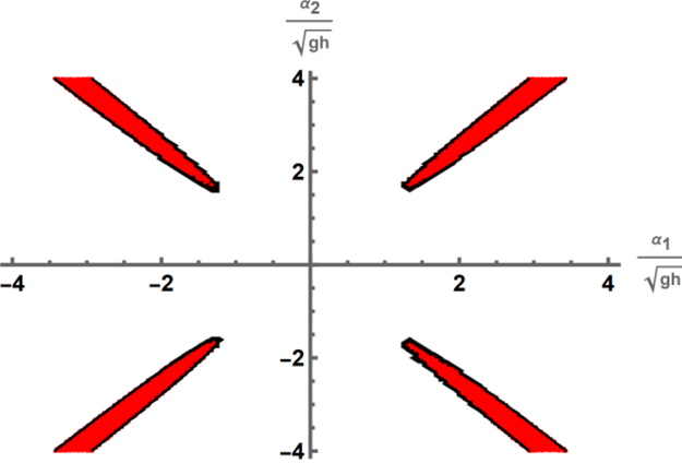
(b) Second order axisymmetric system with full velocity expanded.

Figure 2: Hyperbolicity region of the Second order axisymmetric system with radial velocity expanded (a) and the Second order axisymmetric system with full velocity expanded (b). Red regions indicate loss of hyperbolicity. Compare [12].

Hyperbolicity plots of the systems with radial velocity expanded up to order five have been obtained and they all display a lack of hyperbolicity in some regions. Thus, we conclude that the axisymmetric systems with full velocity expanded are generally not globally hyperbolic. This is no surprise, because a lot of the structure in these systems is inherited from the one-dimensional SWME, see Section 3.

2.3.2 Hyperbolicity breakdown of axisymmetric system with full velocity expanded

Also the axisymmetric systems with full velocity expanded lack global hyperbolicity. This hyperbolicity loss already occurs in the second order system. The system matrix of the second order axisymmetric system with full velocity expanded is given by:

$$A_{A}^{(2,2)}=\begin{pmatrix}0&1&0&0&0&0&0\\ d_{1}&2v_{r,m}&\frac{2\alpha_{1}}{3}&\frac{2\alpha_{2}}{5}&0&0&0\\ d_{2}&2\alpha_{1}&v_{r,m}+\alpha_{2}&\frac{3\alpha_{1}}{5}&0&0&0\\ d_{3}&2\alpha_{2}&\frac{\alpha_{1}}{3}&v_{r,m}+\frac{3\alpha_{2}}{7}&0&0&0\\ \tilde{d}_{1}&v_{\theta,m}&\frac{\gamma_{1}}{3}&\frac{\gamma_{2}}{5}&v_{r,m}&\frac{\alpha_{1}}{3}&\frac{\alpha_{2}}{5}\\ \tilde{d}_{2}&\gamma_{1}&\frac{3\gamma_{2}}{5}&\frac{\gamma_{1}}{5}&\alpha_{1}&v_{r,m}+\frac{2\alpha_{2}}{5}&\frac{2\alpha_{1}}{5}\\ \tilde{d}_{3}&\gamma_{2}&-\frac{\gamma_{1}}{3}&\frac{\gamma_{2}}{7}&\alpha_{2}&\frac{2\alpha_{1}}{3}&v_{r,m}+\frac{2\alpha_{2}}{7}\end{pmatrix},$$ (2.11)

where the entries of the first column are not shown explicitly here for conciseness. They are given in Appendix B. The eigenvalues of $A_{A}^{(2,2)}$ are of the form $\lambda=v_{r,m}+c\sqrt{gh}$, where $c$ is any root of the polynomial

$$-c^{7}+\mathopen{}\mathclose{{}\left(\frac{9\alpha_{1}^{2}}{5}+1}\right)c^{5}+\mathopen{}\mathclose{{}\left(-\frac{23\alpha_{1}^{4}}{25}-\frac{4\alpha_{1}^{2}}{5}}\right)c^{3}+\mathopen{}\mathclose{{}\left(\frac{3\alpha_{1}^{6}}{25}+\frac{3\alpha_{1}^{4}}{25}}\right)c=0.$$

Note that, unlike the matrix $A_{A}^{(2,2)}$ itself, the characteristic polynomial of this matrix and the eigenvalues do not depend on $\gamma_{1}$ and $\gamma_{2}$ due to the lower triangular block structure of $A_{A}^{(2,2)}$.

The loss of hyperbolicity is displayed in Figure 2(b), which shows the hyperbolicity region of the second order axisymmetric system with full velocity expanded. Note that, interestingly, both plots in Figure 2 are identical, implying that the loss of hyperbolicity is induced by the equations for the radial variables $h,hv_{r,m},hv_{\theta,m}$ and $h\alpha_{i}$, with $i=1,\ldots,N_{r}$. Again, the hyperbolicity plot is seemingly identical to the hyperbolicity plot of the one-dimensional second order system [12]. This suggests that the lack of hyperbolicity of the two-dimensional systems is closely related to the hyperbolicity loss of the one-dimensional SWME.

3 Hyperbolic Axisymmetric Shallow Water Moment Equations

As shown in the previous section, the ASWME clearly lack hyperbolicity. In [12], the loss of hyperbolicity of the one-dimensional SWME is overcome by modifying the system matrix, based on a similar approach from kinetic theory [9, 3, 13]. We will extend this idea to the quasi one-dimensional ASWME.

First, note that both the first-order axisymmetric system with radial velocity expanded (i.e. the (1,0)th order system) and the first-order axisymmetric system with full velocity expanded (i.e. the (1,1)th order system) are globally hyperbolic, as can easily be verified using 2.2. The Hyperbolic Axisymmetric Shallow water Moment Equations (HASWME) are derived by linearizing the $(N_{r},N_{\theta})$th order system matrix $A_{A}^{(N_{r},N_{\theta})}$ around linear deviations from the constant equilibrium velocity profile, i.e.,

$$(h,v_{r,m},\alpha_{1},\ldots,\alpha_{N_{r}},v_{\theta,m},\gamma_{1},\ldots,\gamma_{N_{\theta}})\longrightarrow(h,v_{r,m},\alpha_{1},0,\ldots,0,v_{\theta,m},\gamma_{1},0,\ldots,0).$$

Practically, the higher order coefficients $\alpha_{i}$ and $\gamma_{i}$, with $i\geq 2$, are set to zero in the system matrix. This way, the HASWME system with modified system matrix $A_{HA}$ is obtained:

$$\frac{\partial V}{\partial t}+A_{HA}\frac{\partial V}{\partial r}=G(V)+S(V).$$ (3.1)

The analytical forms of the hyperbolic axisymmetric systems with radial velocity expanded and the hyperbolic axisymmetric systems with full velocity expanded can be derived, allowing for deeper mathematical analysis of the HASWME model.

Remark 3.1.

We note that similar to [12] and [11], different ways to perform a hyperbolic regularization exist. Additional regularization terms could be used to construct models with specific eigenvalues. However, we leave this option for potential future work and focus on the standard hyperbolic regularization method here.

3.1 Analytical form of the axisymmetric system with radial velocity expanded

Deriving the full system matrix and then applying the hyperbolic regularization mentioned above, the hyperbolic system matrix is obtained.

Theorem 3.2.

The HASWME system matrix $A_{HA}^{(N_{r},0)}\in\mathbb{R}^{(N_{r}+3)\times(N_{r}+3)}$ is given by

$$A_{HA}^{(N_{r},0)}=\begin{pmatrix}&1&&&&&&\\[6.0pt] gh-v_{r,m}^{2}-\frac{1}{3}\alpha_{1}^{2}&2v_{r,m}&\frac{2}{3}\alpha_{1}&&&&\\[6.0pt] -2v_{r,m}\alpha_{1}&2\alpha_{1}&v_{r,m}&\frac{3}{5}\alpha_{1}&&&&\\[6.0pt] -\frac{2}{3}\alpha_{1}^{2}&&\frac{1}{3}\alpha_{1}&v_{r,m}&\ddots&&&\\[6.0pt] &&&\ddots&\ddots&\frac{N_{r}+1}{2N_{r}+1}\alpha_{1}&\\[6.0pt] &&&&\frac{N_{r}-1}{2N_{r}-1}\alpha_{1}&v_{r,m}&\\[6.0pt] -v_{r,m}v_{\theta,m}&v_{\theta,m}&&&&&v_{r,m}\end{pmatrix},$$ (3.2)

where all other entries are zero.

Proof.

The proof can be found in Appendix A.1. ∎

The structure of the system matrix of the hyperbolic axisymmetric systems with radial velocity expanded is very similar to the structure of the one-dimensional $N_{r}$th order system matrix. There is one additional equation (for $hv_{\theta,m}$) and one additional partial derivative with respect to $hv_{\theta,m}$, compare [14]. This means that the results in [12] can be used to investigate the hyperbolicity of the hyperbolic axisymmetric systems with radial velocity expanded. In particular, the following theorem yields the characteristic polynomial in analytical form.

Theorem 3.3.

The HASWME system matrix $A_{HA}^{(N_{r},0)}\in\mathbb{R}^{(N_{r}+3)\times(N_{r}+3)}$ has the following characteristic polynomial:

$$\chi_{A_{HA}^{(N_{r},0)}}(\lambda)=(\lambda-v_{r,m})\cdot\mathopen{}\mathclose{{}\left(\mathopen{}\mathclose{{}\left(\lambda-v_{r,m})^{2}-gh-\alpha_{1}^{2}}\right)}\right)\cdot\chi_{A_{2}^{(N_{r},0)}}(\lambda-v_{r,m}),$$ (3.3)

where $A_{2}^{(N_{r},0)}\in\mathbb{R}^{N_{r}\times N_{r}}$ is defined as

$$A_{2}^{(N_{r},0)}=\begin{pmatrix}&c_{1}&&\\[6.0pt] a_{2}&&\ddots&\\[6.0pt] &\ddots&&c_{N_{r}-1}\\[6.0pt] &&a_{N_{r}}&\end{pmatrix},$$ (3.4)

where the entries of $A_{2}^{(N_{r},0)}$ are given by

$$a_{i} =\frac{i-1}{2i-1}\alpha_{1}\qquad i=2,\ldots,N_{r},$$ (3.5)

$$c_{i} =\frac{i+2}{2i+3}\alpha_{1}\qquad i=1,\ldots,N_{r}-1.$$ (3.6)

Proof.

The proof can be found in Appendix A.1. ∎

Finally, it is proved that all the hyperbolic axisymmetric systems with radial velocity expanded have real eigenvalues.

Theorem 3.4.

The eigenvalues of the modified hyperbolic axisymmetric system matrix $A_{HA}^{(N_{r},0)}\in\mathbb{R}^{(N_{r}+3)\times(N_{r}+3)}$ are the real numbers

$$\lambda_{1} =v_{r,m},$$ (3.7)

$$\lambda_{2,3} =v_{r,m}\pm\sqrt{gh+\alpha_{1}^{2}},$$ (3.8)

$$\lambda_{i+3} =v_{r,m}+b_{i}\cdot\alpha_{1},\qquad i=1,\ldots,N_{r},$$ (3.9)

with $b_{i}\cdot\alpha_{1}$ the real roots of $A_{2}^{(N_{r},0)}$ from Theorem 3.3 and where all $b_{i}$ are pairwise distinct.

Proof.

The proof can be found in Appendix A.1. ∎

In comparison with the eigenvalues of $N_{r}$th order one-dimensional HSWME, see [12], $\lambda_{1}=v_{r,m}$ is the only new eigenvalue, due to the structure of the system matrix of the axisymmetric equations, which are closely related to the one-dimensional HSWME [12].

Remark 3.5.

Note that for the $N_{r}$th order systems with radial velocity expanded with $N_{r}$ odd, there is an eigenvalue $\lambda=v_{r,m}$ with algebraic multiplicity two. It remains to show that this eigenvalue also has geometric multiplicity two, so that the system matrix is real diagonalizable. In all explicitly computed cases (up to order $(5,0)$), this was the case. A general proof for the special case of $N_{r}$ odd is left for future work.

Corollary 3.1.

If $\alpha_{1}\neq 0$ and if $N_{r}$ is odd, the $N_{r}$th order HASWME with radial velocity expanded are globally hyperbolic.

Proof.

This follows immediately form Theorem 3.4. ∎

The condition that $N_{r}$ is odd is already discussed in Remark 3.5. The first condition, $\alpha_{1}\neq 0$, is a subtle observation and has to do with the multiplicity of the eigenvalues. This will be discussed in more detail in the next section.

3.2 Analytical form of the axisymmetric system with full velocity expanded

The structure of the hyperbolic axisymmetric systems with radial velocity expanded, and thus of the one-dimensional systems in particular, facilitates the derivation of the analytical form of the hyperbolic axisymmetric systems with full velocity expanded. Since there are $N$ additional moment equations and $N$ additional derivatives to be considered, the derivation is more complex than the derivation of the hyperbolic axisymmetric systems with radial velocity expanded. The system matrix of the hyperbolic axisymmetric systems with radial velocity expanded shows a lot of structure.

Theorem 3.6.

The HASWME system matrix $A_{HA}^{(N,N)}\in\mathbb{R}^{(2N+3)\times(2N+3)}$ is given by

$$A_{HA}^{(N,N)}=\begin{pmatrix}\mathbf{A}^{(N,N)}&\mathbf{0}^{(N,N)}\\ \mathbf{B}^{(N,N)}&\mathbf{C}^{(N,N)}\end{pmatrix},$$ (3.10)

where

$$\mathbf{A}^{(N,N)}=\begin{pmatrix}&1&&&&\\[6.0pt] gh-v_{r,m}^{2}-\frac{1}{3}\alpha_{1}^{2}&2v_{r,m}&\frac{2}{3}\alpha_{1}&&&\\[6.0pt] -2v_{r,m}\alpha_{1}&2\alpha_{1}&v_{r,m}&\frac{3}{5}\alpha_{1}&&&\\[6.0pt] -\frac{2}{3}\alpha_{1}^{2}&&\frac{1}{3}\alpha_{1}&v_{r,m}&\ddots&&\\[6.0pt] &&&\ddots&\ddots&\frac{N+1}{2N+1}\alpha_{1}\\[6.0pt] &&&&\frac{N-1}{2N-1}\alpha_{1}&v_{r,m}\end{pmatrix},$$

$$\mathbf{B}^{(N,N)}=\begin{pmatrix}-v_{r,m}v_{\theta,m}-\frac{\alpha_{1}\gamma_{1}}{3}&v_{\theta,m}&\frac{\gamma_{1}}{3}&&&\\[6.0pt] -v_{r,m}\gamma_{1}-v_{\theta,m}\alpha_{1}&\gamma_{1}&&\frac{2}{5}\gamma_{1}&&\\[6.0pt] -\frac{2}{3}\alpha_{1}\gamma_{1}&&-\frac{1}{3}\gamma_{1}&&\ddots&\\[6.0pt] &&&\ddots&\ddots&\frac{N}{2N+1}\gamma_{1}\\[6.0pt] &&&&-\frac{1}{2N-1}\gamma_{1}&\end{pmatrix},$$

$$\mathbf{C}^{(N,N)}=\begin{pmatrix}v_{r,m}&\frac{\alpha_{1}}{3}&&&&\\[6.0pt] \alpha_{1}&v_{r,m}&\frac{2}{5}\alpha_{1}&&&\\[6.0pt] &\frac{2}{3}\alpha_{1}&v_{r,m}&\ddots&&\\[6.0pt] &&\ddots&\ddots&\frac{N}{2N+1}\alpha_{1}\\[6.0pt] &&&\frac{N}{2N-1}\alpha_{1}&v_{r,m}\end{pmatrix},$$

with $\mathbf{A}^{(N,N)}\in\mathbb{R}^{(N+2)\times(N+2)}$, $\mathbf{B}^{(N,N)}\in\mathbb{R}^{(N+1)\times(N+2)}$ and $\mathbf{C}^{(N,N)}\in\mathbb{R}^{(N+1)\times(N+1)}$ and where all other entries are zero. $\mathbf{0}^{(N,N)}\in\mathbb{R}^{(N+2)\times(N+1)}$ is a zero matrix.

Proof.

The proof can be found in Appendix A.2. ∎

In particular, the system matrix is a block lower triangular matrix, simplifying the computation of the characteristic polynomial and the eigenvalues below.

Theorem 3.7.

The HASWME system matrix $A_{HA}^{(N,N)}\in\mathbb{R}^{(N+3)\times(N+3)}$ has the following characteristic polynomial:

$$\chi_{A_{HA}^{(N,N)}}(\lambda)=\mathopen{}\mathclose{{}\left(\mathopen{}\mathclose{{}\left(\lambda-v_{r,m})^{2}-gh-\alpha_{1}^{2}}\right)}\right)\cdot\chi_{A_{2}^{(N,N)}}(\lambda-v_{r,m})\cdot\chi_{A_{3}^{(N,N)}}(\lambda),$$ (3.11)

where $A_{2}^{(N,N)}\in\mathbb{R}^{N\times N}$ and $A_{3}^{(N,N)}\in\mathbb{R}^{(N+1)\times(N+1)}$ are defined as

$$A_{2}^{(N,N)}=\begin{pmatrix}&c_{1}&&\\[6.0pt] a_{2}&&\ddots&\\[6.0pt] &\ddots&&c_{N-1}\\[6.0pt] &&a_{N}&\end{pmatrix},\qquad A_{3}^{(N,N)}=\begin{pmatrix}v_{r,m}&\frac{\alpha_{1}}{3}&&\\[6.0pt] \alpha_{1}&v_{r,m}&g_{1}&&\\[6.0pt] &f_{2}&v_{r,m}&\ddots&\\[6.0pt] &&\ddots&\ddots&g_{N-1}\\[6.0pt] &&&f_{N}&v_{r,m}\end{pmatrix}$$

with

$$a_{i} =\frac{i-1}{2i-1}\alpha_{1},\quad f_{i}=\frac{i}{2i-1}\alpha_{1},\qquad i=2,\ldots,N,$$

$$c_{i} =\frac{i+2}{2i+3}\alpha_{1},\quad g_{i}=\frac{i+1}{2i+3}\alpha_{1},\qquad i=1,\ldots,N-1.$$

Proof.

The proof can be found in Appendix A.2. ∎

Note that the matrix $A_{2}^{(N,N)}$ in Theorem 3.7 is the same matrix as defined in Theorem 3.3 but with a slightly different notation adjusted to the different setting.

Theorem 3.8.

The eigenvalues of the modified axisymmetric hyperbolic system matrix $A_{HA}^{(N,N)}\in\mathbb{R}^{(2N+3)\times(2N+3)}$ are the real numbers

$$\lambda_{1,2} =v_{r,m}\pm\sqrt{gh+\alpha_{1}^{2}},$$ (3.12)

$$\lambda_{i+2} =v_{r,m}+b_{i}\alpha_{1},\qquad i=1,\ldots,N,$$ (3.13)

$$\lambda_{i+2+N} =v_{r,m}+s_{i}\alpha_{1},\qquad i=1,\ldots,N+1,$$ (3.14)

with $b_{i}\cdot\alpha_{1}$ the real roots of $A_{2}^{(N,N)}$, and $s_{i}\cdot\alpha_{1}$ the real roots of $A_{3}^{(N,N)}$, from Theorem 3.7 and where all the $b_{i}$’s and the $s_{i}$’s are pairwise distinct.

Proof.

The proof can be found in Appendix A.2. ∎

Remark 3.9.

According to Theorem 3.8, the roots of the system matrix of a hyperbolic axisymmetric system with full velocity expanded are real. However, for vanishing first coefficient $\alpha_{1}$ all eigenvalues (3.13) and (3.14) are equal to $v_{r,m}$. To have hyperbolicity in this case, the eigenspace spanned by the eigenvalues needs to have the same dimension as the multiplicity of the eigenvalue. The same observation is made in the hyperbolic axisymmetric systems with radial velocity expanded, see Theorem 3.4; the eigenvalues 3.9 collide when $\alpha_{1}=0$. A direct numerical computation reveals that the hyperbolic axisymmetric systems with radial velocity expanded are hyperbolic at least up to order $N_{r}=5$, but the hyperbolic axisymmetric system with full velocity expanded are not hyperbolic for order $N=1,2,3,4,5$.

Remark 3.9 suggests a condition for the hyperbolic axisymmetric systems with full velocity expanded to be hyperbolic.

Corollary 3.2.

If $\alpha_{1}\neq 0$, the $N$th order HASWME with full velocity expanded are globally hyperbolic.

Proof.

This follows immediately from Theorem 3.2. ∎

Remark 3.10.

The construction of the $N_{r}$th order systems with radial velocity expanded and the $N$th order systems with full velocity expanded allow for a generalization to arbitrary systems with order of expansion $N_{r}$ in radial direction and order of expansion $N_{\theta}$ in angular direction, with $N_{r}\neq N_{\theta}\neq 0$. A straightforward extension of the theory is that the system matrix will always be a lower triangular matrix, facilitating the computation of the characteristic polynomial considerably. Denoting the blocks of the system matrix by

$$\mathbf{A}_{sys}=\begin{pmatrix}\mathbf{A}&\mathbf{0}\\[5.0pt] \mathbf{B}&\mathbf{C}\end{pmatrix},$$

the matrix $\mathbf{A}$ corresponds to the system matrix in the one-dimensional HSWME [12]. Moreover, the dimension of this matrix is only determined by the radial order $N_{r}$. Since the matrix $\mathbf{B}$ is lower triangular, block $\mathbf{B}$, which contains the derivatives with respect to $h,v_{r,m}$ and $\alpha_{i}$, with $i\in[1,2,\ldots,N_{r}]$, that appear in the angular momentum balance equation and the equations for $\gamma_{i}$, with $i\in[1,2,\ldots,N_{\theta}]$, does not appear in the calculation of the characteristic polynomial. Block $\mathbf{C}$ contains the derivatives with respect to $v_{\theta,m}$ and $\gamma_{i}$, with $i\in[1,2,\ldots,N_{\theta}]$, that appear in the angular momentum balance equation and the equations for $\gamma_{i}$, with $i\in[1,2,\ldots,N_{\theta}]$. Therefore, the dimension of block $\mathbf{C}$ only depends on the angular order $N_{\theta}$. It follows that matrix $\mathbf{C}$ is precisely the matrix $C^{(N_{\theta},N_{\theta})}$ defined in Theorem 3.6. In particular, this means that the hyperbolicity theorems and proofs given in Appendix A.1 and A.2 can be easily generalized to systems with order $N_{r}$ in radial direction and order $N_{\theta}$ in angular direction.

Remark 3.11.

The stability properties of the HASWME (3.1) are not solely determined by the system matrix representing the transport part, but also by the dissipation part of the model, which is inscribed in the right-hand side source terms [23, 10]. An equilibrium stability analysis of the one-dimensional HSWME is performed in [10], in which equilibrium manifolds of the one-dimensional models are derived and in which a set of stability conditions, proposed in [23], is verified for each of these manifolds. For the HASWME, the forcing terms denoted by $G(V)$ in (3.1) pose mathematical difficulties, for the analytically derivation of explicit expressions for the equilibrium manifolds. The equilibrium analysis is therefore left for future work.

4 Numerical Simulation

In this section, we first show that the HASWME overcome the stability problems of the ASWME by considering a dam break situation. Then, we demonstrate that the ASWME and the HASWME yield accurate results by considering a test case with smooth initial conditions. Moreover, we observe that, in general, the error reduces with respect to increasing order $N$ throughout all models. The simulations are performed using the axisymmetric systems with full velocity expanded up to order $N=4$. Simulations with axisymmetric moment models with radial velocity expanded are left to future work.

Numerical simulations were performed with the ASWME and the HASWME. An important feature of the cylindrical SWME that has to be dealt with are the forcing terms, because they contain a factor $1/r$. This causes a singularity for $r\to 0$. There are two ways to overcome this problem: The first option is to multiply the reference equations (2.5)-(2.7) with $r$ and then proceed in the same way as before. The second option is to exclude the singularity $r\to 0$ from the domain. In this paper, we opted for the second approach and we performed numerical simulations on a mesh with $r$-domain $[1,10]$.

We note that the runtime of the HASWME is smaller than the runtime of the ASWME, as the number of non linear terms is reduced because of the hyperbolic modification of the system matrix.

The numerical solutions were computed using the first order non-conservative PRICE scheme and the software framework also employed for the simulations in [8]. The reference solutions were obtained using the software accompanying [14].

4.1 Radial dam break

First, a test case with a discontinuous initial height profile will be considered. The numerical setup can be found in Table 1. This setup is very similar to the 1D test case with discontinuous initial data in [12]. The initial radial velocity is a cubic function of the height, while the initial angular velocity is zero at every point in the domain. The initial height function takes the form of a scenario in which there is a circular dam in the middle of the flow. The simulations are performed using the third order axisymmetric model with full velocity expanded and the third order hyperbolic axisymmetric model with full velocity expanded. Simulations with end times $t=0.1$ and $t=0.3$ are performed and the results are plotted in 3. The values of the variables are not plotted for the whole domain, but only in that part of the domain in which there are significant differences between the different approximations.

$\nu$	$\nu=0.1$
$\lambda$	$\lambda=0.1$
Spatial domain	$r\in[10,20],\quad y\in[0,2\pi]$
$t_{end}$	$t_{end}\in\{0.1,0.3\}$
$h(r,\theta,0)$	$$h(r,\theta,0)=\begin{cases}5.0,&r\leq 14.0\\ 1.0,&r>14.0\end{cases}$$
$v_{r}(r,\theta,\zeta,0)$	$v_{r}(r,\theta,\zeta,0)=0.25-2.5\zeta+7.5\zeta^{2}-5\zeta^{3}$
$v_{\theta}(r,\theta,\zeta,0)$	$v_{\theta}(r,\theta,\zeta,0)=0$
Time integration	Forward Euler
Spatial discretization	PRICE scheme
CFL number	0.1

Table 1: Numerical setup for radial dam break scenario.

Figure 3(a) and 3(b) show that the ASWME and the HASWME yield similar and accurate results for the water height $h$. The same can be observed for the radial mean velocity $v_{r,m}$, shown in Figure 3(c) and Figure 3(d). For the approximation of the first coefficient $\alpha_{1}$, the ASWME and the HASWME give qualitatively different results, as seen in 3(e) and 3(f). At time $t=0.1$, the HASWME outperforms the ASWME, as the latter model displays an oscillation that is not present in the reference solution. This is in agreement with the numerical results obtained in [12], in which an instability was observed in the numerical simulation of the 1D SWME. However, at time $t=0.3$, which was not previously reported in the comparable test case in [12], both the ASWME and the HASWME approximations are not accurate compared to the reference solution, so it is not straightforward to argument if one model is more accurate than the other. In conclusion, the hyperbolic model is preferred at shorter times, while it is not clear which model is preferred at larger times.

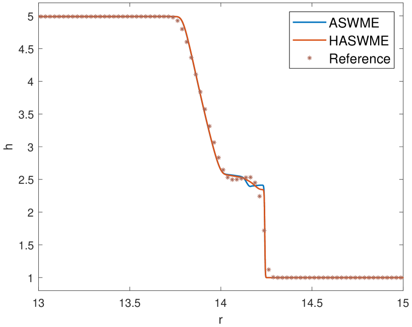
(a) $h$ at time $t=0.1$

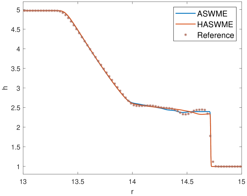
(b) $h$ at time $t=0.3$

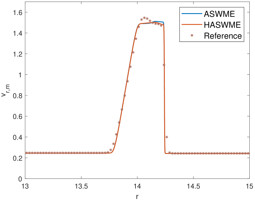
(c) $v_{r,m}$ at time $t=0.1$

(d) $v_{r,m}$ at time $t=0.3$

(e) $\alpha_{1}$ at time $t=0.1$

(f) $\alpha_{1}$ at time $t=0.3$

Figure 3: Test case with discontinuous initial height profile for the third order ASWME and HASWME with full velocity expanded at times $t=0.1$ and $t=0.3$. The ASWME and the HASWME yield almost identical results.

4.2 Smooth initial height profile

Next, we consider a test case with a smooth initial height profile. The numerical setup is given in Table 2. The setup is closely related to the 1D smooth test case considered in [12], but a slightly different initial height function and a different initial velocity profile are used. The initial height function takes the form of a reverse sigmoid function. The initial radial velocity is zero everywhere, while the initial angular velocity is $v_{\theta}(r,\theta,\zeta,0)=0.5$ and does not depend on the spatial variables.

$\nu$	$\nu=1$
$\lambda$	$\lambda=0.1$
Spatial domain	$r\in[10,20],\quad y\in[0,2\pi]$
$t_{end}$	$t_{end}=0.5$
$h(r,\theta,0)$	$h(r,\theta,0)=1+\frac{4}{1+e^{2(r-14)}}$
$v_{r}(r,\theta,\zeta,0)$	$v_{r}(r,\theta,\zeta,0)=0$
$v_{\theta}(r,\theta,\zeta,0)$	$v_{\theta}(r,\theta,\zeta,0)=0.5$
Time integration	Forward Euler
Spatial discretization	PRICE scheme
CFL number	0.1

Table 2: Numerical setup for smooth test case.

Moment approximations are obtained using the ASWME and the HASWME $N$th order models with full velocity expanded, with $N\in\{0,1,2,3\}$. Again, the numerical solution is only displayed for a fraction of the radial space. The results are shown in 4. The values of $h$, $v_{r,m}$ and $v_{\theta,m}$ are plotted for both the ASWME model (left column) and the HASWME model (right column) with increasing order $N$. Figure 4(a) and Figure 4(b) show that the approximations for the water height $h$ are more accurate with increasing order, compared to the reference solution. This is the case for both the ASWME models and the HASWME models. This trend is also clearly visible for the mean angular velocity, see Figure 4(e) and 4(f). For the mean radial velocity, displayed in Figure 4(c) and 4(d), the zeroth order model and the first order model are less accurate than the higher order models. However, it appears that the second order model is more accurate than the third order model in this part of the domain. Nevertheless, the error of the third order model is smaller than the error of the second order model, because the former model gives a better approximation than the latter in a large part of the domain, which is not displayed in Figure 4(c) and Figure 4(d).

The error convergence is shown in Figure 5, which shows the relative error of the different models for the water height $h$, the mean radial velocity $v_{r,m}$ and the mean angular velocity $v_{\theta,m}$. For all three variables, we observe a reduction of the error when the order increases from $N=0$ to $N=3$. In particular, the error in the ASWE model with $N=0$ is considerably larger than the error in both moment models ASWME and HASWME for $N>0$. This is in agreement with the 1D results in [12]. However, when the order is increased from $N=3$ to $N=4$, there is no reduction in the error anymore for most of the models. It is not clear what the cause of this stagnation can be. In any case, the error is already small in the third order model, especially for $h$ and $v_{\theta,m}$. We can conclude that for this smooth test case, the moment models yield approximations that are increasingly accurate when the order of the model increase. This is the case for both the non-hyperbolic and the hyperbolic models.

(a) $h$ at time $t=0.5$

(b) $h$ at time $t=0.5$

(c) $v_{r,m}$ at time $t=0.5$

(d) $v_{r,m}$ at time $t=0.5$

(e) $v_{\theta,m}$ at time $t=0.5$

(f) $v_{\theta,m}$ at time $t=0.5$

Figure 4: Test case with reverse sigmoid initial height profile for different orders $(N,N)$ and the (2,2)th and $(3,3)$th order HASWME at time $t=0.5$. The accuracy of the approximations increases with increasing order. The ASWME (left column) and the HASWME (right column) yield very similar results.

Figure 5: Error convergence of smooth test case for ASWME and HASWME.

5 Conclusion

In this paper we derived the first hyperbolic moment models for shallow flow in cylindrical coordinate systems. The paper started with a brief review of the derivation of the SWME. The reference system was then transformed to cylindrical coordinates and ASWME were derived for axisymmetric flow. We showed the breakdown of hyperbolicity of the ASWME by means of hyperbolicity plots. This lead to the derivation of the first hyperbolic axisymmetric model called HASWME for which we showed hyperbolicity using an in-depth analysis of the system matrix. In the numerical simulation of a test case with discontinuous initial height profile, the hyperbolic model resulted in a more accurate approximation compared to a reference solution. The numerical simulation of a test case with smooth initial data showed that the approximation error decreases when the order of the model is increased. Moreover, both the HASWME and the ASWME showed to be accurate approximations with respect to a reference solution. We conclude that the ASWME and the HASWME are two successful models for the simulation of free surface flow. Although a lot of the structure of the equations is inherited from the 1D equations, they allow for the simulation of 2D axisymmetric flow. The models can therefore be seen as an intermediate stage between the 1D and 2D models.

Ongoing work focuses on the extension of the axisymmetric models to moment models that are fully 2D and the numerical simulation of these models. Another point of interest would be to perform an equilibrium stability analysis of the ASWME and the HASWME. A final suggestion for future work is the derivation of tailored numerical methods for the axisymmetric models.

Data Availability Statement

The datasets generated and analysed during this study are available from the corresponding author on reasonable request.

Appendix A Hyperbolicity Proof For HASWME

A.1 Axisymmetric system with radial velocity expanded

Theorem A.1.

The HASWME system matrix $A_{HA}^{(N_{r},0)}\in\mathbb{R}^{(N_{r}+3)\times(N_{r}+3)}$ is given by

$$A_{HA}^{(N_{r},0)}=\begin{pmatrix}&1&&&&&&\\[6.0pt] gh-v_{r,m}^{2}-\frac{1}{3}\alpha_{1}^{2}&2v_{r,m}&\frac{2}{3}\alpha_{1}&&&&\\[6.0pt] -2v_{r,m}\alpha_{1}&2\alpha_{1}&v_{r,m}&\frac{3}{5}\alpha_{1}&&&&\\[6.0pt] -\frac{2}{3}\alpha_{1}^{2}&&\frac{1}{3}\alpha_{1}&v_{r,m}&\ddots&&&\\[6.0pt] &&&\ddots&\ddots&\frac{N_{r}+1}{2N_{r}+1}\alpha_{1}&\\[6.0pt] &&&&\frac{N_{r}-1}{2N_{r}-1}\alpha_{1}&v_{r,m}&\\[6.0pt] -v_{r,m}v_{\theta,m}&v_{\theta,m}&&&&&v_{r,m}\end{pmatrix},$$ (A.1)

where all other entries are zero.

Proof.

The matrix $A_{HA}^{(N_{r},0)}$ is obtained by computing $A_{A}^{(N_{r},0)}$, the full system matrix, and then setting the higher order moments to zero [12]. We derive the rows of the system matrix separately:

1. Mass and radial momentum balance equations. The first two rows of the system matrix correspond to the mass balance and the radial momentum balance equations. It can be easily seen that the first two rows of the coefficient matrix are

$$\begin{pmatrix}&1&&&&&\\[6.0pt] gh-v_{r,m}^{2}-\frac{1}{3}\alpha_{1}^{2}+\sum_{i=1}^{N_{r}}\alpha_{i}^{2}&2v_{r,m}&\frac{2}{3}\alpha_{1}&\frac{2}{5}\alpha_{2}&\cdots&\frac{2}{2N_{r}+1}\alpha_{N}&0\end{pmatrix}.$$

After setting the higher order moments to zero, we obtain

$$\begin{pmatrix}&1&&&&&\\[6.0pt] gh-v_{r,m}^{2}-\frac{1}{3}\alpha_{1}^{2}&2v_{r,m}&\frac{2}{3}\alpha_{1}&&&&\end{pmatrix}.$$

2. Angular momentum balance equation. The last row of the coefficient matrix corresponds to the angular momentum balance equation. Recall the flux in this equation $F_{N_{r}+3}:=hv_{r,m}v_{\theta,m}$. It can be easily verified that

$$\frac{\partial F_{N_{r}+3}}{\partial h}=-v_{r,m}v_{\theta,m},\quad\frac{\partial F_{N_{r}+3}}{\partial(hv_{r,m})}=v_{\theta,m},\quad\frac{\partial F_{N_{r}+3}}{\partial(h\alpha_{l})}=0,\quad\frac{\partial F_{N_{r}+3}}{\partial(hv_{\theta,m})}=v_{r,m}.$$

3. The equations for $\alpha_{i},i=1,\ldots,N_{r}$. The equation for the $i$th moment reads

$$\frac{\partial(h\alpha_{i})}{\partial t}+\frac{\partial F_{i}}{\partial r}=Q_{i}+P_{i}.$$

The system matrix $A_{H}^{(N_{r},0)}$ is composed of a conservative and a non-conservative part.

3.1 The conservative part $\frac{\partial F_{i}}{\partial r}$. Recall that

$$F_{i} =h\mathopen{}\mathclose{{}\left(2v_{r,m}\alpha_{i}+\sum_{j,k=1}^{N_{r}}A_{ijk}\alpha_{j}\alpha_{k}}\right)=h2v_{r,m}\alpha_{i}+h\sum_{j,k=1}^{N_{r}}(2i+1)\mathopen{}\mathclose{{}\left(\int_{0}^{1}\phi_{i}\phi_{j}\phi_{k}d\zeta}\right)\alpha_{j}\alpha_{k}.$$

Consider the first term, $h2v_{r,m}\alpha_{i}$. With $\boldsymbol{\alpha}=(\alpha_{1},\cdots,\alpha_{N_{r}})$, it can be easily seen (after setting the higher coefficients to zero) that this term leads to

$$\frac{\partial 2hv_{r,m}\boldsymbol{\alpha}}{\partial V}=\begin{pmatrix}-2v_{r,m}\alpha_{1}&2\alpha_{1}&2v_{r,m}&&&\\[6.0pt] &&&\ddots&&\\[6.0pt] &&&&2v_{r,m}&\end{pmatrix}.$$

Now, we look at the second term, with the triple Legendre integral. We call this term $\tilde{F_{i}}:=h\sum_{j,k=1}^{N_{r}}A_{ijk}\alpha_{j}\alpha_{k}$. In [12], it is shown that if $j=1$, the only cases that need to be considered are $k=i-1$ (if $i\geq 2$) and $k=i+1$. Analogously, if $k=1$, the only cases we need to consider are $j=i-1$ (if $i\geq 2$) and $j=i+1$. According to this observations, we can distinguish four different situations.

3.1.1 Case 1: $i=1$. If $i=1$, there are two cases for the index triplet $(i,j,k)$, with $j=1$ or $k=1$, which lead to a non-zero term: $(1,1,2)\text{ and }(1,2,1)$.

So we can pull these cases outside of the sum and we get:

$$\tilde{F_{1}}=\sum_{j,k=1}^{N_{r}}A_{1jk}\alpha_{j}\alpha_{k}=2A_{112}h\alpha_{1}\alpha_{2}+h\sum_{j,k=2}^{N_{r}}A_{1jk}\alpha_{j}\alpha_{k}.$$

The factor $2$ appears because both index triplets lead to the same term.

The derivative of the second term with respect to $h$ reads

$$\frac{\partial\mathopen{}\mathclose{{}\left(h\sum_{j,k=2}^{N_{r}}A_{1jk}\alpha_{j}\alpha_{k}}\right)}{\partial h}=-\sum_{j,k=2}^{N_{r}}A_{1jk}\alpha_{j}\alpha_{k}.$$

After setting the higher order moments to zero, this term reduces to zero. The same can be observed when taking the derivative with respect to $hv_{r,m}$, $h\alpha_{l}$ (with $l=1,\cdots,N_{r}$) and $hv_{\theta,m}$.

The derivatives of the first term read

$$\frac{\partial(2A_{112}h\alpha_{1}\alpha_{2})}{\partial(h\alpha_{l})}=2A_{112}\alpha_{1}\delta_{2,l}+2A_{112}\alpha_{2}\delta_{1,l}.$$

When we set higher order moments to zero, the second term vanishes. We call the resulting entry $c_{1}^{F}$. This entry corresponds to the derivative with respect to $h\alpha_{2}$ and will be discussed later. All other derivatives are zero, except the derivative with respect to $h$, but we can easily see that this derivative reduces to zero when we set higher order moments to zero.

3.1.2 Case 2: $i=2$. There are three cases for the index triplet $(i,j,k)$, with $j=1$ or $k=1$, which lead to a non-zero term: $(2,1,1),(2,1,3),\text{ and }(2,3,1)$.

We can pull these terms outside of the sum:

$$\tilde{F_{2}}=\sum_{j,k=1}^{N_{r}}A_{2jk}\alpha_{j}\alpha_{k}=A_{211}h\alpha_{1}^{2}+2A_{213}h\alpha_{1}\alpha_{3}+h\sum_{j,k=2}^{N_{r}}A_{2jk}\alpha_{j}\alpha_{k}.$$

Again, the derivatives of the last term all reduce to zero when setting the higher order moments to zero. Denoting the first and the second term by $\underline{\tilde{F}_{2}}:=A_{211}h\alpha_{1}^{2}+2A_{213}h\alpha_{1}\alpha_{3}$, we have:

$$\frac{\partial\underline{\tilde{F}_{2}}}{\partial(h\alpha_{l})}=2A_{211}\alpha_{1}\delta_{1,l}+2A_{213}\alpha_{1}\delta_{3,l}+2A_{213}\alpha_{3}\delta_{1,l}.$$

Setting higher order moments to zero, this reduces to

$$2A_{211}\alpha_{1}\delta_{1,l}+2A_{213}\alpha_{1}\delta_{3,l}.$$

The first term leads to an entry $a_{2}^{F}$. The second term leads to an entry $c_{2}^{F}$. In the same way, one can easily see that

$$\frac{\partial\underline{\tilde{F}_{2}}}{\partial h}=-A_{211}\alpha_{1}^{2}-\alpha_{1}\alpha_{3},\quad\frac{\partial\underline{\tilde{F}_{2}}}{\partial(hv_{r,m})}=0,\quad\frac{\partial\underline{\tilde{F}_{2}}}{\partial(hv_{\theta,m})}=0.$$

When higher order moment are set to zero, this only results in a term $-\frac{2}{3}\alpha_{1}^{2}$ in the first column.

3.1.3 Case 3: $2<i\leq N_{r}-1$. In this case, there are four possibilities for the index triplet $(i,j,k)$: $(i,1,i-1),(i,1,i+1),(i,i-1,1),\text{ and }(i,i+1,1)$.

We can pull this terms outside of the sum:

$$\tilde{F_{i}}=\sum_{j,k=1}^{N_{r}}A_{ijk}\alpha_{j}\alpha_{k}=2A_{i,1,i-1}h\alpha_{1}\alpha_{i-1}+2A_{i,1,i+1}h\alpha_{1}\alpha_{i+1}+h\sum_{j,k=2}^{N_{r}}A_{ijk}\alpha_{j}\alpha_{k}.$$

The derivatives of the last term all reduce to zero when setting the higher order moments to zero. Denoting the rest by $\underline{\tilde{F}_{i}}:=2A_{i,1,i-1}h\alpha_{1}\alpha_{i-1}+2A_{i,1,i+1}h\alpha_{1}\alpha_{i+1}$ yields

$$\frac{\partial\underline{\tilde{F}_{i}}}{\partial(h\alpha_{l})}=2A_{i,1,i-1}\alpha_{1}\delta_{i-1,l}+2A_{i,1,i-1}\alpha_{i-1}\delta_{1,l}+2A_{i,1,i+1}\alpha_{1}\delta_{i+1,l}+2A_{i,1,i+1}\alpha_{i+1}\delta_{1,l}.$$

Setting higher order moments to zero, this reduces to

$$2A_{i,1,i-1}\alpha_{1}\delta_{i-1,l}+2A_{i,1,i+1}\alpha_{1}\delta_{i+1,l}.$$

The first term leads to an entry $a_{i}^{F}$. The second term leads to an entry $c_{i}^{F}$. For the other derivatives, it is again easy to see that

$$\frac{\partial\underline{\tilde{F}_{i}}}{\partial h}=-2A_{i,1,i-1}\alpha_{1}\alpha_{i-1}-\alpha_{1}\alpha_{i+1},\quad\frac{\partial\underline{\tilde{F}_{i}}}{\partial(hv_{r,m})}=0,\quad\frac{\partial\underline{\tilde{F}_{i}}}{\partial(hv_{\theta,m})}=0.\\$$

When higher order moments are set to zero, the derivative with respect to $h$ reduces to zero.

3.1.4 Case 4: $i=N_{r}$. In this case, there are two possibilities for the index triplet $(i,j,k)$: $(N_{r},1,N_{r}-1)\text{ and }(N_{r},N_{r}-1,1)$.

Analogously to the previous cases, it can be easily shown that this equation only leads to an entry $a_{N_{r}}^{F}$ in the $(N_{r}-1)$th column of the $(N_{r}+2)$th row, the row corresponding to the equation for the $N_{r}$th moment.

Using orthogonality and recursion formulas (see also [12]), we have:

$$a_{i}^{F}=\frac{2i}{2i-1}\alpha_{1},\qquad i=2,\ldots,N_{r},$$

$$c_{i}^{F}=\frac{2i+2}{2i+3}\alpha_{1},\qquad i=1,\ldots,N_{r}-1.$$

The entry $a_{i}^{F}$ corresponds to a derivative with respect to $h\alpha_{i-1}$ and is located on the first lower diagonal. The entry $c_{i}^{F}$ corresponds to a derivative with respect to $h\alpha_{i+1}$ and is located on the first upper diagonal leading to the modified flux derivative $\frac{\partial F}{\partial V}_{mod}$:

$$\frac{\partial F}{\partial V}_{mod}=\begin{pmatrix}&1&&&&&&\\[6.0pt] gh-v_{r,m}^{2}-\frac{1}{3}\alpha_{1}^{2}&2v_{r,m}&\frac{2}{3}\alpha_{1}&&&&\\[6.0pt] -2v_{r,m}\alpha_{1}&2\alpha_{1}&2v_{r,m}&c_{1}^{F}&&&&\\[6.0pt] -\frac{2}{3}\alpha_{1}^{2}&&a_{2}^{F}&2v_{r,m}&\ddots&&&\\[6.0pt] &&&\ddots&\ddots&c_{N_{r}-1}^{F}&\\[6.0pt] &&&&a_{N_{r}}^{F}&2v_{r,m}&\\[6.0pt] -v_{r,m}v_{\theta,m}&v_{\theta,m}&&&&&v_{r,m}\end{pmatrix}$$ (A.2)

3.2 The non-conservative part $Q_{i}$. Recall the non-conservative part in the equation for $h\alpha_{i}$:

$$Q_{i}=v_{r,m}\frac{\partial(h\alpha_{i})}{\partial r}-\sum_{j,k=1}^{N_{r}}B_{ijk}\alpha_{k}\frac{\partial(h\alpha_{j})}{\partial r}.$$ (A.3)

Clearly, the first term leads to the term $v_{r,m}$ on the diagonal of $Q$. The second term is simplified when we set higher order moments to zero:

$$-\sum_{j=1}^{N_{r}}(2i+1)\mathopen{}\mathclose{{}\left(\int_{0}^{1}\phi_{i}^{\prime}\mathopen{}\mathclose{{}\left(\int_{0}^{1}\phi_{j}d\hat{\zeta}}\right)\phi_{1}d\zeta}\right)\alpha_{1}\frac{\partial(h\alpha_{j})}{\partial r}.$$

It can be proved that $B_{ij1}=0$ for $|i-j|\neq 1$, except for the first two rows. $Q_{i}$ does not depend on any derivative with respect to $h,hv_{r,m}$ and $hv_{\theta,m}$, so the entries of the corresponding columns will be zero. The entries of the first two rows and the last row are also all zero; the mass and momentum balances do not contain non-conservative terms. By considering three different cases ($i=1$, $1<i\leq N_{r}-1$ and $i=N_{r}$) in an analogous way as for the conservative terms, we can see that the second term in (A.3) only leads to non-zero entries $a_{i}^{Q}$ on the first lower diagonal and non-zero entries $c_{i}^{Q}$ on the first upper diagonal:

$$a_{i}^{Q}=\frac{i+1}{2i-1}\alpha_{1}\qquad i=2,\ldots,N_{r},$$

$$c_{i}^{Q}=\frac{i}{2i+3}\alpha_{1}\qquad i=1,\ldots,N_{r}-1.$$

This results in the following non-conservative part $Q_{mod}$:

$$Q_{mod}=\begin{pmatrix}&&&&&&&\\[6.0pt] &&&&&&&\\[6.0pt] &&&v_{r,m}&c_{1}^{Q}&&&\\[6.0pt] &&&a_{2}^{Q}&v_{r,m}&\ddots&&\\[6.0pt] &&&&\ddots&\ddots&c_{N_{r}-1}^{Q}&\\[6.0pt] &&&&&a_{N_{r}}^{Q}&v_{r,m}&\\[6.0pt] &&&&&&&\end{pmatrix}$$ (A.4)

The modified system matrix is given by

$$A_{HA}^{(N_{r},0)}=\frac{\partial F}{\partial V}_{mod}-Q_{mod}.$$

This completes the proof. ∎

Theorem A.2.

The HASWME system matrix $A_{HA}^{(N_{r},0)}\in\mathbb{R}^{(N_{r}+3)\times(N_{r}+3)}$ has the following characteristic polynomial:

$$\chi_{A_{HA}^{(N_{r},0)}}(\lambda)=(\lambda-v_{r,m})\cdot\mathopen{}\mathclose{{}\left(\mathopen{}\mathclose{{}\left(\lambda-v_{r,m})^{2}-gh-\alpha_{1}^{2}}\right)}\right)\cdot\chi_{A_{2}^{(N_{r},0)}}(\lambda-v_{r,m}),$$ (A.5)

where $A_{2}^{(N_{r},0)}\in\mathbb{R}^{N_{r}\times N_{r}}$ is defined as

$$A_{2}^{(N_{r},0)}=\begin{pmatrix}&c_{1}&&\\[6.0pt] a_{2}&&\ddots&\\[6.0pt] &\ddots&&c_{N_{r}-1}\\[6.0pt] &&a_{N_{r}}&\end{pmatrix},$$ (A.6)

where

$$a_{i} =\frac{i-1}{2i-1}\alpha_{1},\qquad i=2,\ldots,N_{r},$$ (A.7)

$$c_{i} =\frac{i+2}{2i+3}\alpha_{1},\qquad i=1,\ldots,N_{r}-1,$$ (A.8)

are the values below and above the diagonal, respectively.

Proof.

The characteristic polynomial of the modified system matrix $A_{HA}^{(N_{r},0)}$ is by definition

$$\chi_{A_{HA}^{(N_{r},0)}}(\lambda)=\det(A_{HA}^{(N_{r},0)}-\lambda I):=\lvert A_{HA}^{(N_{r},0)}-\lambda I\rvert.$$

First, we develop with respect to the first column:

$$\qquad\lvert A_{HA}^{(N_{r},0)}-\lambda I\rvert=\\[7.0pt] \begin{vmatrix}-\lambda&1&&&&&&\\[6.0pt] gh-v_{r,m}^{2}-\frac{1}{3}\alpha_{1}^{2}&2v_{r,m}-\lambda&\frac{2}{3}\alpha_{1}&&&&\\[6.0pt] -2v_{r,m}\alpha_{1}&2\alpha_{1}&v_{r,m}-\lambda&\frac{3}{5}\alpha_{1}&&&&\\[6.0pt] -\frac{2}{3}\alpha_{1}^{2}&&\frac{1}{3}\alpha_{1}&v_{r,m}-\lambda&\ddots&&&\\[6.0pt] &&&\ddots&\ddots&\frac{N_{r}+1}{2N_{r}+1}\alpha_{1}&\\[6.0pt] &&&&\frac{N_{r}-1}{2N_{r}-1}\alpha_{1}&v_{r,m}-\lambda&\\[6.0pt] -v_{r,m}v_{\theta,m}&v_{\theta,m}&&&&&v_{r,m}-\lambda\\ \end{vmatrix}\\[11.0pt] =(v_{r,m}-\lambda)\cdot\underbrace{\begin{vmatrix}&1&&&&&\\[6.0pt] gh-v_{r,m}^{2}-\frac{1}{3}\alpha_{1}^{2}&2v_{r,m}&\frac{2}{3}\alpha_{1}&&&\\[6.0pt] -2v_{r,m}\alpha_{1}&2\alpha_{1}&v_{r,m}&\frac{3}{5}\alpha_{1}&&&\\[6.0pt] -\frac{2}{3}\alpha_{1}^{2}&&\frac{1}{3}\alpha_{1}&v_{r,m}&\ddots&&\\[6.0pt] &&&\ddots&\ddots&\frac{N_{r}+1}{2N_{r}+1}\alpha_{1}\\[6.0pt] &&&&\frac{N_{r}-1}{2N_{r}-1}\alpha_{1}&v_{r,m}\end{vmatrix}.}_{=:\lvert A_{1}^{(N_{r},0)}\rvert}$$

In [12], it is proved that

$$\chi_{A_{1}^{(N_{r},0)}}(\lambda)=\mathopen{}\mathclose{{}\left(\mathopen{}\mathclose{{}\left(\lambda-v_{r,m})^{2}-gh-\alpha_{1}^{2}}\right)}\right)\cdot\chi_{A_{2}^{(N_{r},0)}}(\lambda-v_{r,m}),$$

with $A_{2}^{(N_{r},0)}$ as in (A.6). Note that in [12], $u_{m}$ is used instead of $v_{r,m}$. This completes the proof. ∎

Corollary A.1.

The eigenvalues of the one-dimensional radial system matrix are also eigenvalues of the modified axisymmetric hyperbolic system matrix $A_{HA}^{(N_{r},0)}$. Moreover, the only additional eigenvalue of $A_{HA}^{(N_{r},0)}$ is $\lambda=v_{r,m}$.

Proof.

This follows immediately from the Theorem A.2. ∎

Corollary A.2.

The eigenvalues of the modified hyperbolic axisymmetric system matrix $A_{HA}^{(N_{r},0)}\in\mathbb{R}^{(N_{r}+3)\times(N_{r}+3)}$ are the real numbers.

$$\lambda_{1}=v_{r,m},\quad\lambda_{2,3}=v_{r,m}\pm\sqrt{gh+\alpha_{1}^{2}},\lambda_{i+3}=v_{r,m}+b_{i}\cdot\alpha_{1},\qquad i=1,\ldots,N_{r},$$

with $b_{i}\cdot\alpha_{1}$ the real roots of $A_{2}^{(N_{r},0)}$, defined in (A.6), and where all $b_{i}$ are pairwise distinct.

Proof.

According to A.2, the characteristic polynomial of $A_{HA}^{(N_{r},0)}$ is given by:

$$\chi_{A_{HA}^{(N_{r},0)}}(\lambda)=(\lambda-v_{r,m})\cdot\mathopen{}\mathclose{{}\left(\mathopen{}\mathclose{{}\left(\lambda-v_{r,m})^{2}-gh-\alpha_{1}^{2}}\right)}\right)\cdot\chi_{A_{2}^{(N_{r},0)}}(\lambda-v_{r,m}).$$

From the first factor, we can immediately see that $\lambda_{1}=v_{r,m}$. From the second factor, we easily obtain $\lambda_{2,3}=v_{r,m}\pm\sqrt{gh+\alpha_{1}^{2}}$.

In [12], it is shown that the roots of $\chi_{A_{2}^{(N_{r},0)}}(\lambda-v_{r,m})$ have the form $\lambda_{i}=v_{r,m}+b_{i}\cdot\alpha_{1}$, where all $b_{i}$ are pairwise distinct. Moreover, in [10] it is proved that the roots are real. ∎

A.2 Axisymmetric system with full velocity expanded

Theorem A.3.

The HASWME system matrix $A_{HA}^{(N,N)}\in\mathbb{R}^{(2N+3)\times(2N+3)}$ is given by

$$A_{HA}^{(N,N)}=\begin{pmatrix}\mathbf{A}^{(N,N)}&\mathbf{0}^{(N,N)}\\ \mathbf{B}^{(N,N)}&\mathbf{C}^{(N,N)}\end{pmatrix},$$ (A.9)

where the blocks are given by

$$\mathbf{A}^{(N,N)}=\begin{pmatrix}&1&&&&\\[6.0pt] gh-v_{r,m}^{2}-\frac{1}{3}\alpha_{1}^{2}&2v_{r,m}&\frac{2}{3}\alpha_{1}&&&\\[6.0pt] -2v_{r,m}\alpha_{1}&2\alpha_{1}&v_{r,m}&\frac{3}{5}\alpha_{1}&&&\\[6.0pt] -\frac{2}{3}\alpha_{1}^{2}&&\frac{1}{3}\alpha_{1}&v_{r,m}&\ddots&&\\[6.0pt] &&&\ddots&\ddots&\frac{N+1}{2N+1}\alpha_{1}\\[6.0pt] &&&&\frac{N-1}{2N-1}\alpha_{1}&v_{r,m}\end{pmatrix},$$

$$\mathbf{B}^{(N,N)} =\begin{pmatrix}-v_{r,m}v_{\theta,m}-\frac{\alpha_{1}\gamma_{1}}{3}&v_{\theta,m}&\frac{\gamma_{1}}{3}&&&\\[6.0pt] -v_{r,m}\gamma_{1}-v_{\theta,m}\alpha_{1}&\gamma_{1}&&\frac{2}{5}\gamma_{1}&&\\[6.0pt] -\frac{2}{3}\alpha_{1}\gamma_{1}&&-\frac{1}{3}\gamma_{1}&&\ddots&\\[6.0pt] &&&\ddots&\ddots&\frac{N}{2N+1}\gamma_{1}\\[6.0pt] &&&&-\frac{1}{2N-1}\gamma_{1}&\end{pmatrix},$$

$$\mathbf{C}^{(N,N)} =\begin{pmatrix}v_{r,m}&\frac{\alpha_{1}}{3}&&&&\\[6.0pt] \alpha_{1}&v_{r,m}&\frac{2}{5}\alpha_{1}&&&\\[6.0pt] &\frac{2}{3}\alpha_{1}&v_{r,m}&\ddots&&\\[6.0pt] &&\ddots&\ddots&\frac{N}{2N+1}\alpha_{1}\\[6.0pt] &&&\frac{N}{2N-1}\alpha_{1}&v_{r,m}\end{pmatrix},$$

with $\mathbf{A}^{(N,N)}\in\mathbb{R}^{(N+2)\times(N+2)}$, $\mathbf{B}^{(N,N)}\in\mathbb{R}^{(N+1)\times(N+2)}$ and $\mathbf{C}^{(N,N)}\in\mathbb{R}^{(N+1)\times(N+1)}$ and where all other entries are zero. $\mathbf{0}^{(N,N)}\in\mathbb{R}^{(N+2)\times(N+1)}$ is a zero matrix.

Proof.

The matrix $A_{HA}^{(N,N)}$ is obtained by computing $A_{A}^{(N,N)}$, the full system matrix, and then setting the higher order moments to zero similar to [12]. The computation of the matrix entries is analogous to the proof of Theorem A.1, so we proceed in the same way.

1. First $2+N$ equations. The first $N+2$ equations correspond to the mass and the radial momentum balance equations and the equations for $h\alpha_{i}$ ($i=1,\ldots,N$). The conservative flux and the non-conservative flux in these equations are exactly the same as for the $(N_{r},0)$th order systems, so we can use the results of Theorem A.1. Furthermore, the conservative flux and the non-conservative flux in all these equations do not depend on the angular moment $h\gamma_{i}$ ($i=1,\ldots,N$). With this observations, it is clear that the first $2+N$ rows of the matrix are given by

$$\begin{pmatrix}&1&0&\cdots&&&&&0\\[6.0pt] gh-v_{r,m}^{2}-\frac{1}{3}\alpha_{1}^{2}&2v_{r,m}&\frac{2}{3}\alpha_{1}&0&\cdots&&&&0\\[6.0pt] -2v_{r,m}\alpha_{1}&2\alpha_{1}&v_{r,m}&\frac{3}{5}\alpha_{1}&0&\cdots&&&0\\[6.0pt] -\frac{2}{3}\alpha_{1}^{2}&&\frac{1}{3}\alpha_{1}&v_{r,m}&\ddots&0&\cdots&&0\\[6.0pt] &&&\ddots&\ddots&\frac{N_{r}+1}{2N_{r}+1}\alpha_{1}&0&\cdots&0\\[6.0pt] &&&&\frac{N_{r}-1}{2N_{r}-1}\alpha_{1}&v_{r,m}&0&\cdots&0\end{pmatrix}.$$

2. Angular momentum balance equation. The $(N+3)$th row of the coefficient matrix corresponds to the angular momentum balance equation. Recall the flux in this equation is

$$F_{N_{r}+3}:=hv_{r,m}v_{\theta,m}+h\sum_{j=1}^{N}\frac{\alpha_{j}\gamma_{j}}{2j+1}.$$

It can be easily verified that

$$\frac{\partial F_{N_{r}+3}}{\partial h}=-v_{r,m}v_{\theta,m}-\sum_{j=1}^{N}\frac{\alpha_{j}\gamma_{j}}{2j+1}\quad\stackrel{{\scriptstyle\mathclap{\mbox{{lin}}}}}{{=}}\quad-v_{r,m}v_{\theta,m}-\frac{\alpha_{1}\gamma_{1}}{3},$$

$$\frac{\partial F_{N_{r}+3}}{\partial(hv_{r,m})}=v_{\theta,m}\quad\stackrel{{\scriptstyle\mathclap{\mbox{{lin}}}}}{{=}}\quad v_{\theta,m},\quad\frac{\partial F_{N_{r}+3}}{\partial(h\alpha_{l})}=\frac{\gamma_{l}}{2l+1}\quad\stackrel{{\scriptstyle\mathclap{\mbox{{lin}}}}}{{=}}\quad\frac{\gamma_{l}}{2l+1}\delta_{1,l},$$

$$\frac{\partial F_{N_{r}+3}}{\partial(hv_{\theta,m})}=v_{r,m}\quad\stackrel{{\scriptstyle\mathclap{\mbox{{lin}}}}}{{=}}\quad v_{r,m},\quad\frac{\partial F_{N_{r}+3}}{\partial(h\gamma_{l})}=\frac{\alpha_{l}}{2l+1}\quad\stackrel{{\scriptstyle\mathclap{\mbox{{lin}}}}}{{=}}\quad\frac{\alpha_{l}}{2l+1}\delta_{1,l},$$

where $\quad\stackrel{{\scriptstyle\mathclap{\mbox{{lin}}}}}{{=}}\quad$ is setting the higher order moments to zero.

3. The equations for $\boldsymbol{\gamma_{i}},i=1,\ldots,N$. The equation for the $i$th moment is given by

$$\frac{\partial(h\gamma_{i})}{\partial t}+\frac{\partial F_{i}}{\partial r}=Q_{i}+P_{i}.$$

The system matrix $A_{H}^{(N,N)}$ is composed of a conservative and a non-conservative part.

3.1 The conservative part $\frac{\partial F_{i}}{\partial r}$. Recall that

$$F_{i} =h\mathopen{}\mathclose{{}\left(v_{r,m}\gamma_{i}+v_{\theta,m}\alpha_{i}+\sum_{j,k=1}^{N_{r}}A_{ijk}\alpha_{j}\gamma_{k}}\right)$$ (A.10)

$$=hv_{r,m}\gamma_{i}+hv_{\theta,m}\alpha_{i}+h\sum_{j,k=1}^{N_{r}}(2i+1)\mathopen{}\mathclose{{}\left(\int_{0}^{1}\phi_{i}\phi_{j}\phi_{k}d\zeta}\right)\alpha_{j}\gamma_{k}.$$ (A.11)

Consider the first term in the right-hand side in Equation (A.11), $hv_{r,m}\gamma_{i}$. Clearly, this term does not depend on $\alpha_{l}$ ($l=1,\ldots,N$) and on $v_{\theta,m}$, so all the derivatives with respect to $h\alpha_{l}$ and $v_{\theta,m}$ will be zero. Furthermore, we have:

$$\frac{\partial hv_{r,m}\gamma_{i}}{\partial h}=-v_{r,m}\gamma_{i},\quad\frac{\partial hv_{r,m}\gamma_{i}}{\partial(hv_{r,m})}=\gamma_{i},\quad\frac{\partial hv_{r,m}\gamma_{i}}{\partial(h\gamma_{l})}=v_{r,m}\delta_{i,l}.$$

Then we consider the second term in the right-hand side in Equation (A.11), $hv_{\theta,m}\alpha_{i}$. This term does not depend on $\gamma_{l}$ ($l=1,\ldots,N$) and on $hv_{\theta,m}$, so all the derivatives with respect to $h\gamma_{l}$ and with respect to $hv_{\theta,m}$ will be zero. Furthermore, we have:

$$\frac{\partial hv_{\theta,m}\alpha_{i}}{\partial h}=-v_{\theta,m}\alpha_{i},\quad\frac{\partial hv_{\theta,m}\alpha_{i}}{\partial(hv_{\theta,m})}=\alpha_{i},\quad\frac{\partial hv_{\theta,m}\alpha_{i}}{\partial(h\alpha_{l})}=v_{\theta,m}\delta_{i,l}.$$

Introducing the notation

$$V_{\boldsymbol{\alpha}}:=(h,hv_{r,m},h\alpha_{1},\cdots,h\alpha_{N}),\quad V_{\boldsymbol{\gamma}}:=(hv_{\theta,m},h\gamma_{1},\cdots,h\alpha_{N}),$$

with $\boldsymbol{\alpha}=(\alpha_{1},\cdots,\alpha_{N})$ and with $\boldsymbol{\gamma}=(\gamma_{1},\cdots,\gamma_{N})$, we obtain

$$\frac{\partial(hv_{r,m}\boldsymbol{\gamma}+hv_{\theta,m}\boldsymbol{\alpha})}{\partial V_{\boldsymbol{\alpha}}}\quad\stackrel{{\scriptstyle\mathclap{\mbox{{lin}}}}}{{=}}\quad\begin{pmatrix}-v_{r,m}\gamma_{1}-v_{\theta,m}\alpha_{1}&\gamma_{1}&v_{\theta,m}&&\\[6.0pt] &&&\ddots&\\[6.0pt] &&&&v_{\theta,m}\end{pmatrix},$$

$$\frac{\partial(hv_{r,m}\boldsymbol{\gamma}+hv_{\theta,m}\boldsymbol{\alpha})}{\partial V_{\boldsymbol{\gamma}}}\quad\stackrel{{\scriptstyle\mathclap{\mbox{{lin}}}}}{{=}}\quad\begin{pmatrix}\alpha_{1}&v_{r,m}&&\\[6.0pt] &&\ddots&\\[6.0pt] &&&v_{r,m}\end{pmatrix}.$$

We denote the last term of the right-hand side of Equation (A.11) with the triple Legendre integral as $\tilde{F_{i}}:=h\sum_{j,k=1}^{N}A_{ijk}\alpha_{j}\alpha_{k}$. In [12], it is shown that if $j=1$, the only cases that need to be considered are $k=i-1$ (if $i\geq 2$) and $k=i+1$. Analogously, if $k=1$, the only cases we need to consider are $j=i-1$ (if $i\geq 2$) and $j=i+1$. Analogously to the corresponding section in the proof of Theorem A.1, we can consider four different situations.

3.1.1 Case 1: $i=1$. If $i=1$, there are two cases for the index triplet $(i,j,k)$, with $j=1$ or $k=1$, which lead to a non-zero term: $(1,1,2)\text{ and }(1,2,1)$.

So we can pull these cases outside of the sum and we get:

$$\tilde{F_{1}}=\sum_{j,k=1}^{N}A_{ijk}\alpha_{j}\gamma_{k}=A_{112}h\alpha_{1}\gamma_{2}+A{121}h\alpha_{2}\gamma_{1}+h\sum_{j,k=2}^{N}A_{ijk}\alpha_{j}\gamma_{k}.$$

The derivative of the last term with respect to $h$ reads

$$\frac{\partial\mathopen{}\mathclose{{}\left(h\sum_{j,k=2}^{N}A_{ijk}\alpha_{j}\alpha_{k}}\right)}{\partial h}=-\sum_{j,k=2}^{N}A_{ijk}\alpha_{j}\gamma_{k}.$$

After setting the higher order moments to zero, this term reduces to zero. The same can be observed when taking the derivative with respect to $hv_{r,m}$, $h\alpha_{l}$ and $h\gamma_{l}$ ($l=1,\ldots,N$) and $hv_{\theta,m}$.

The derivative of the first and second term denoted as $\underline{\tilde{F_{1}}}:=A_{112}h\alpha_{1}\gamma_{2}+A_{121}h\alpha_{2}\gamma_{1}$ are

$$\frac{\partial\underline{\tilde{F_{1}}}}{\partial(h\alpha_{l})} =A_{112}\gamma_{2}\delta_{1,l}+A_{112}\gamma_{1}\delta_{2,l}\quad\stackrel{{\scriptstyle\mathclap{\mbox{{lin}}}}}{{=}}\quad A_{112}\gamma_{1}\delta_{2,l},$$

$$\frac{\partial\underline{\tilde{F_{1}}}}{\partial(h\gamma_{l})} =A_{112}\alpha_{1}\delta_{2,l}+A_{112}\alpha_{2}\delta_{1,l}\quad\stackrel{{\scriptstyle\mathclap{\mbox{{lin}}}}}{{=}}\quad A_{112}\alpha_{1}\delta_{2,l}.$$

We denote the resulting entries ${}_{\alpha}c_{1}^{F}$ and ${}_{\gamma}c_{1}^{F}$, respectively. All other derivatives are zero, except for the derivative with respect to $h$, but we can easily see that this derivative reduces to zero when we set higher order moments to zero.

3.1.2 Case 2: $i=2$. Now, there are three cases for the index triplet $(i,j,k)$, with $j=1$ or $k=1$, which lead to a non-zero term: $(2,1,1),(2,1,3),\text{ and }(2,3,1)$.

We can pull this terms outside of the sum:

$$\tilde{F_{2}}=\sum_{j,k=1}^{N}A_{ijk}\alpha_{j}\gamma_{k}=A_{211}h\alpha_{1}\gamma_{1}+A_{213}h\alpha_{1}\gamma_{3}+A_{231}h\alpha_{3}\gamma_{1}+h\sum_{j,k=2}^{N}A_{ijk}\alpha_{j}\gamma_{k}.$$ (A.12)

Again, the derivatives of the last term in the right-hand side of Equation (A.12) all reduce to zero when setting the higher order moments to zero. Denoting the first three terms by $\underline{\tilde{F}_{2}}:=A_{211}h\alpha_{1}\gamma_{1}+A_{213}h\alpha_{1}\gamma_{3}+A_{231}h\alpha_{3}\gamma_{1}$, we obtain

$$\frac{\partial\underline{\tilde{F}_{2}}}{\partial(h\alpha_{l})}\quad\stackrel{{\scriptstyle\mathclap{\mbox{{lin}}}}}{{=}}\quad A_{211}\gamma_{1}\delta_{1,l}+A_{213}\gamma_{1}\delta_{1,3},\quad\frac{\partial\underline{\tilde{F}_{2}}}{\partial(h\gamma_{l})}\quad\stackrel{{\scriptstyle\mathclap{\mbox{{lin}}}}}{{=}}\quad A_{211}\alpha_{1}\delta_{1,l}+A_{213}\alpha_{1}\delta_{3,l}.$$

Considering the left equation, the first term leads to an entry ${}_{\alpha}a_{2}^{F}$ and the second term leads to an entry ${}_{\alpha}c_{2}^{F}$. Considering the right equation, the first term leads to an entry ${}_{\gamma}a_{2}^{F}$ and the second term leads to an entry ${}_{\gamma}c_{2}^{F}$. Regarding the other derivatives, one can easily see that

$$\frac{\partial\underline{\tilde{F}_{2}}}{\partial h}\quad\stackrel{{\scriptstyle\mathclap{\mbox{{lin}}}}}{{=}}\quad-A_{211}\alpha_{1}\gamma_{1}-\alpha_{1}\gamma_{3},~{}\frac{\partial\underline{\tilde{F}_{2}}}{\partial(hv_{r,m})}=0,~{}\frac{\partial\underline{\tilde{F}_{2}}}{\partial(hv_{\theta,m})}=0.$$

3.1.3 Case 3: $2<i\leq N-1$. In this case, there are four possibilities for the index triplet $(i,j,k)$: $(i,1,i-1),(i,1,i+1),(i,i-1,1),\text{ and }(i,i+1,1)$.

We can pull this terms outside of the sum:

$$\tilde{F_{i}}=\sum_{j,k=1}^{N}A_{ijk}\alpha_{j}\gamma_{k}\\ =A_{i,1,i-1}h\alpha_{1}\gamma_{i-1}+A_{i,1,i+1}h\alpha_{1}\gamma_{i+1}+A_{i,i-1,1}h\alpha_{i-1}\gamma_{1}+A_{i,i+1,1}h\alpha_{i+1}\gamma_{1}+h\sum_{j,k=2}^{N}A_{ijk}\alpha_{j}\gamma_{k}.$$ (A.13)

The derivatives of the last term of the right-hand side of Equation (A.13) all reduce to zero when setting the higher order moments to zero. Denoting the other terms by $\underline{\tilde{F}_{i}}:=A_{i,1,i-1}h\alpha_{1}\gamma_{i-1}+A_{i,1,i+1}h\alpha_{1}\gamma_{i+1}+A_{i,i-1,1}h\alpha_{i-1}\gamma_{1}+A_{i,i+1,1}h\alpha_{i+1}\gamma_{1}$, we obtain

$$\frac{\partial\underline{\tilde{F}_{i}}}{\partial(h\alpha_{l})}\quad \stackrel{{\scriptstyle\mathclap{\mbox{{lin}}}}}{{=}}\quad A_{i,1,i-1}\gamma_{1}\delta_{i-1,l}+A_{i,1,i+1}\gamma_{i+1}\delta_{i+1,l},$$

$$\frac{\partial\underline{\tilde{F}_{i}}}{\partial(h\gamma_{l})}\quad \stackrel{{\scriptstyle\mathclap{\mbox{{lin}}}}}{{=}}\quad A_{i,1,i-1}\alpha_{1}\delta_{i-1,l}+A_{i,1,i+1}\alpha_{i+1}\delta_{i+1,l}.$$

Considering the first equation, the first term leads to an entry ${}_{\alpha}a_{i}^{F}$, while the second term leads to en entry ${}_{\alpha}c_{i}^{F}$. Analogously, the first term of the second equation leads to an entry ${}_{\gamma}a_{i}^{F}$ and the second term of the second equation leads to an entry ${}_{\gamma}a_{i}^{F}$.

To summarize, the ${}_{\alpha}a_{i}^{F}$’s and the ${}_{\alpha}c_{i}^{F}$ correspond to derivatives with respect to $h\alpha_{i-1}$ and with respect to $h\alpha_{i+1}$ of the conservative flux in the equation for $\gamma_{i}$, respectively. The ${}_{\gamma}a_{i}^{F}$’s and the ${}_{\gamma}c_{i}^{F}$ correspond to derivatives with respect to $h\gamma_{i-1}$ and with respect to $h\gamma_{i+1}$ of the conservative flux in the equation for $\gamma_{i}$, respectively.

Furthermore, we find:

$$\frac{\partial\underline{\tilde{F}_{i}}}{\partial h}\quad\stackrel{{\scriptstyle\mathclap{\mbox{{lin}}}}}{{=}}\quad 0,\quad\frac{\partial\underline{\tilde{F}_{i}}}{\partial(hv_{r,m})}\quad\stackrel{{\scriptstyle\mathclap{\mbox{{lin}}}}}{{=}}\quad 0,\quad\frac{\partial\underline{\tilde{F}_{i}}}{\partial(hv_{\theta,m})}\quad\stackrel{{\scriptstyle\mathclap{\mbox{{lin}}}}}{{=}}\quad 0.\\$$

3.1.4 Case 4: $i=N$. In this case, there are two possibilities for the index triplet $(i,j,k)$: $(N,1,N-1)\text{ and }(N,N-1,1)$.

Analogously to the previous cases, it can be easily shown that this case only leads to entries ${}_{\alpha}a_{N}^{F}$, ${}_{\alpha}c_{N}^{F}$, ${}_{\gamma}a_{N}^{F}$ and ${}_{\gamma}c_{N}^{F}$.

Using orthogonality and recursion formulas, we have:

$${}_{\alpha}a_{i}^{F}=\frac{i}{2i-1}\gamma_{1}\qquad\text{and}\qquad_{\gamma}a_{i}^{F}=\frac{i}{2i-1}\alpha_{1},\qquad i=2,\ldots,N,$$

$${}_{\alpha}c_{i}^{F}=\frac{i+1}{2i+3}\gamma_{1}\qquad\text{and}\qquad_{\gamma}c_{i}^{F}=\frac{i+1}{2i+3}\alpha_{1},\qquad i=1,\ldots,N-1.$$

In conclusion, we have for the modified conservative coefficient matrix:

$$\frac{\partial F}{\partial V_{\alpha}}_{mod}=\begin{pmatrix}&1&&&&&\\[6.0pt] gh-v_{r,m}^{2}-\frac{1}{3}\alpha_{1}^{2}&2v_{r,m}&\frac{2}{3}\alpha_{1}&&&\\[6.0pt] -2v_{r,m}\alpha_{1}&2\alpha_{1}&2v_{r,m}&c_{1}^{F}&&&\\[6.0pt] -\frac{2}{3}\alpha_{1}^{2}&&a_{2}^{F}&2v_{r,m}&\ddots&&\\[6.0pt] &&&\ddots&\ddots&c_{N-1}^{F}&\\[6.0pt] &&&&a_{N}^{F}&2v_{r,m}\\[6.0pt] -v_{r,m}v_{\theta,m}-\frac{\alpha_{1}\gamma_{1}}{3}&v_{\theta,m}&\frac{\gamma_{1}}{3}&&&\\[6.0pt] -v_{r,m}\gamma_{1}-v_{\theta,m}\alpha_{1}&\gamma_{1}&v_{\theta,m}&{}_{\alpha}c_{1}^{F}&&\\[6.0pt] -\frac{2}{3}&&{}_{\alpha}a_{2}^{F}&v_{\theta,m}&\ddots&\\[6.0pt] &&&\ddots&\ddots&{}_{\alpha}c_{N-1}^{F}\\[6.0pt] &&&&{}_{\alpha}a_{N}^{F}&v_{\theta,m}\end{pmatrix},$$

$$\frac{\partial F}{\partial V_{\gamma}}_{mod}=\begin{pmatrix}&&&&&\\[6.0pt] &&&&&\\[6.0pt] &&&&&\\[6.0pt] &&&&&\\[6.0pt] &&&&&\\[6.0pt] &&&&&\\[6.0pt] v_{r,m}&\frac{\alpha_{1}}{3}&&&\\[6.0pt] \alpha_{1}&v_{r,m}&{}_{\gamma}c_{1}^{F}&\\[6.0pt] &{}_{\gamma}a_{2}^{F}&v_{r,m}&\ddots&\\[6.0pt] &&\ddots&\ddots&{}_{\gamma}c_{N-1}^{F}\\[6.0pt] &&&{}_{\gamma}a_{N}^{F}&v_{r,m}\end{pmatrix}.$$

3.2 The non-conservative part $Q_{i}$. The non-conservative part in the equations for $h,hv_{r,m}$ and $h\alpha_{i}$, $i=1,\ldots,N$, does not depend on derivatives with respect to $h\gamma_{l}$, $l=1,\ldots,N$. Recall the non-conservative part in the equation for $h\gamma_{i}$:

$$Q_{i}=v_{\theta,m}\frac{\partial(h\alpha_{i})}{\partial r}-\sum_{j,k=1}^{N_{r}}B_{ijk}\gamma_{k}\frac{\partial(h\alpha_{j})}{\partial r}.$$ (A.14)

Thus, the equations for $h\gamma_{i}$, $i=1,\ldots,N$, do not depend on derivatives with respect to $h\gamma_{l}$, $l=1,\ldots,N$, either. From this, it follows that we can write the modified non-conservative terms (i.e., with higher order moments set to zero) as

$$Q_{mod}=\begin{pmatrix}Q_{1}&Q_{2}\\ Q_{3}&Q_{4}\end{pmatrix},$$

in which $Q_{2}\in\mathbb{R}^{(N+3)\times N}$ and $Q_{4}\in\mathbb{R}^{N\times N}$ are zero matrices. $Q_{1}\in\mathbb{R}^{(N+3)\times(N+3)}$ is the coefficient matrix of the non-conservative flux in the $(N,0)$th order system, see Equation (A.4) in the proof of Theorem A.1. The remaining entries to compute are the entries of the matrix $Q_{3}\in\mathbb{R}^{N\times(N+3)}$. This matrix corresponds to the equation for $\gamma_{i}$, $i=1,\ldots,n$, and to the derivatives with respect to $h,hv_{r,m}$ and $h\alpha_{l}$ ($l=1,\ldots,N)$. The first term of the non-conservative flux leads to the term $v_{\theta,m}$ on the diagonal of $Q_{3}$. The second term is simplified when we set higher order moments to zero:

$$\sum_{j=1}^{N}(2i+1)\mathopen{}\mathclose{{}\left(\int_{0}^{1}\phi_{i}^{\prime}\mathopen{}\mathclose{{}\left(\int_{0}^{1}\phi_{j}d\hat{\zeta}}\right)\phi_{1}d\zeta}\right)\gamma_{1}\frac{\partial(h\alpha_{j})}{\partial r}.$$

It can be proved that $B_{ij1}=0$ for $|i-j|\neq 1$, except for the first two rows. $Q_{i}$ does not depend on any derivative with respect to $h$, $hv_{r,m}$ and $hv_{\theta,m}$, so the entries of the corresponding columns will be zero. Analogously to the proof of Theorem A.1, we can see that the second term in (A.14) only leads to non-zero entries $a_{i}^{Q}$ on the first lower diagonal and non-zero entries $c_{i}^{Q}$ on the first upper diagonal:

$$a_{i}^{Q}=\frac{i+1}{2i-1}\gamma_{1},\qquad i=2,\ldots,N,$$

$$c_{i}^{Q}=\frac{i}{2i+3}\gamma_{1},\qquad i=1,\ldots,N-1.$$

So $Q_{3}$ has the following form:

$$Q_{3}=\begin{pmatrix}&&&v_{r,m}&c_{1}^{Q}&&\\[6.0pt] &&&a_{2}^{Q}&v_{r,m}&\ddots&&\\[6.0pt] &&&&\ddots&\ddots&c_{N_{r}-1}^{Q}&\\[6.0pt] &&&&&a_{N_{r}}^{Q}&v_{r,m}&\\[6.0pt] \end{pmatrix}.$$

From this, the matrix $Q_{mod}$ can be constructed and the modified system matrix is

$$A_{HA}^{(N,N)}=\frac{\partial_{F}}{\partial V}_{mod}-Q_{mod}.$$

This completes the proof. ∎

Theorem A.4.

The HASWME system matrix $A_{HA}^{(N,N)}\in\mathbb{R}^{(N+3)\times(N+3)}$ has the following characteristic polynomial:

$$\chi_{A_{HA}^{(N,N)}}(\lambda)=\mathopen{}\mathclose{{}\left(\mathopen{}\mathclose{{}\left(\lambda-v_{r,m})^{2}-gh-\alpha_{1}^{2}}\right)}\right)\cdot\chi_{A_{2}^{(N,N)}}(\lambda-v_{r,m})\cdot\chi_{A_{3}^{(N,N)}}(\lambda),$$ (A.15)

where $A_{2}^{(N,N)}\in\mathbb{R}^{N\times N}$ and $A_{3}^{(N,N)}\in\mathbb{R}^{(N+1)\times(N+1)}$ are defined as

$$A_{2}^{(N,N)}=\begin{pmatrix}&c_{1}&&\\[6.0pt] a_{2}&&\ddots&\\[6.0pt] &\ddots&&c_{N_{r}-1}\\[6.0pt] &&a_{N_{r}}&\end{pmatrix},\qquad A_{3}^{(N,N)}=\begin{pmatrix}v_{r,m}&\frac{\alpha_{1}}{3}&&\\[6.0pt] \alpha_{1}&v_{r,m}&g_{1}&&\\[6.0pt] &f_{2}&v_{r,m}&\ddots&\\[6.0pt] &&\ddots&\ddots&g_{N-1}\\[6.0pt] &&&f_{N}&v_{r,m}\end{pmatrix},$$ (A.16)

where the entries are given by

$$a_{i} =\frac{i-1}{2i-1}\alpha_{1}\qquad\text{and}\qquad f_{i}=\frac{i}{2i-1}\alpha_{1},\qquad i=2,\ldots,N,$$

$$c_{i} =\frac{i+3}{2i+3}\alpha_{1}\qquad\text{and}\qquad g_{i}=\frac{i+1}{2i+3}\alpha_{1},\qquad i=1,\ldots,N-1,$$

Proof.

The characteristic polynomial of the modified system matrix $A_{H}^{(N,N)}$ is by definition

$$\chi_{A_{HA}^{(N,N)}}(\lambda)=\det(A_{HA}^{(N,N)}-\lambda I):=\lvert A_{HA}^{(N,N)}-\lambda I\rvert.$$

Recall that the system matrix has the following form:

$$A_{HA}^{(N,N)}=\begin{pmatrix}\mathbf{A^{(N,N)}}&\mathbf{0}\\ \mathbf{B^{(N,N)}}&\mathbf{C^{(N,N)}}\end{pmatrix},$$

where the explicit form of the blocks $\boldsymbol{A^{(N,N)}},\boldsymbol{B^{(N,N)}}$ and $\boldsymbol{C^{(N,N)}}$ is given in Theorem A.9. This is a lower triangular block matrix. It is known that the determinant of a triangular block matrix is given by the determinant of its diagonal blocks, see e.g. [18]. So we have:

$$\lvert A_{HA}^{(N,N)}-\lambda I\rvert=\lvert A^{(N,N)}-\lambda I\rvert\cdot\lvert C^{(N,N)}-\lambda I\rvert.$$

According to [14], the first factor yields:

$$\lvert A^{(N,N)}-\lambda I\rvert=\mathopen{}\mathclose{{}\left(\mathopen{}\mathclose{{}\left(\lambda-v_{r,m})^{2}-gh-\alpha_{1}^{2}}\right)}\right)\cdot\chi_{A_{2}^{(N,N)}}(\lambda-v_{r,m}).$$

The observation that $\mathbf{C}$ is exactly the matrix $A_{3}^{(N,N)}$ as defined above completes the proof. ∎

Lemma A.1.

Let $A\in\mathbb{R}^{n\times n}$ and $D=diag(d_{1},\cdots,d_{n})\in\mathbb{R}^{n\times n}$, with $d_{i}\neq 0$ ($i=1,\cdots,n$). Then $A$ and $DAD^{-1}$ have the same eigenvalues.

Proof.

The proof is not given here. ∎

Lemma A.2.

Let $A\in\mathbb{R}^{n\times n}$ be a real tridiagonal matrix such that $a_{i,i+1}a_{i+1,i}>0$, $i=1,\ldots,n-1$. Then there is a real diagonal matrix $D$ such that $DAD^{-1}$ is symmetric.

Proof.

The proof is not given here. ∎

Corollary A.3.

The eigenvalues of the modified axisymmetric hyperbolic system matrix $A_{HA}^{(N,N)}\in\mathbb{R}^{(2N+3)\times(2N+3)}$ are the real numbers

$$\lambda_{1,2} =v_{r,m}\pm\sqrt{gh+\alpha_{1}^{2}},$$

$$\lambda_{i+2} =v_{r,m}+b_{i}\cdot\alpha_{1},\qquad i=1,\ldots,N,$$

$$\lambda_{i+2+N} =v_{r,m}+s_{i}\cdot\alpha_{1},\qquad i=1,\ldots,N+1.$$

with $b_{i}\cdot\alpha_{1}$ the real roots of $A_{2}^{(N,N)}$, and $s_{i}\cdot\alpha_{1}$ the real roots of $A_{3}^{(N,N)}$, from Theorem A.4 and where all the $b_{i}$’s and the $s_{i}$’s are pairwise distinct.

Proof.

Recall that the characteristic polynomial of $A_{HA}^{(N,N)}$ is given by

$$\chi_{A_{HA}^{(N,N)}}(\lambda)=\mathopen{}\mathclose{{}\left(\mathopen{}\mathclose{{}\left(\lambda-v_{r,m})^{2}-gh-\alpha_{1}^{2}}\right)}\right)\cdot\chi_{A_{2}^{(N,N)}}(\lambda-v_{r,m})\cdot\chi_{A_{3}^{(N,N)}}(\lambda).$$

From the first factor, we easily obtain

$$\lambda_{1,2}=v_{r,m}\pm\sqrt{gh+\alpha_{1}^{2}}.$$

In [14], it is shown that the roots of $\chi_{A_{2}^{(N,N)}}(\lambda-v_{r,m})$ have the form $\lambda_{i}=v_{r,m}+b_{i}\cdot\alpha_{1}$. Moreover, it is proved in [10] that the roots are real.

It remains to prove that the eigenvalues of the matrix $A_{3}^{(N,N)}$ are real. For $\alpha_{1}=0$, it is obvious that all the eigenvalues are real. If $\alpha_{1}\neq 0$, it follows from Lemma A.1 that there is a real diagonal matrix $D$ such that $DAD^{-1}$ is symmetric. Since a symmetric matrix has real eigenvalues, it follows from Lemma A.2 that all the eigenvalues of $A_{3}^{(N,N)}$ are real. This completes the proof. ∎

Appendix B System Matrix Of Second Order Axisymmetric System With Full Velocity Expanded

The entries in the first column of the system matrix of the $(2,2)$th order ASWME system in Equation (2.11) are given by:

$$d_{1} =gh-v_{r,m}^{2}-\frac{\alpha_{1}^{2}}{3}-\frac{\alpha_{2}^{2}}{5},$$

$$d_{2} =-v_{r,m}-\frac{4}{5}\alpha_{1}\alpha_{2},$$

$$d_{3} =-\frac{2}{21}\mathopen{}\mathclose{{}\left(3\alpha_{2}\mathopen{}\mathclose{{}\left(7v_{r,m}+\alpha_{2}}\right)+7\alpha_{1}^{2}}\right),$$

$$\tilde{d}_{1} =-v_{r,m}v_{\theta,m}-\frac{1}{3}\alpha_{1}\gamma_{1}-\frac{\alpha_{2}\gamma_{2}}{5},$$

$$\tilde{d}_{2} =\frac{1}{5}\mathopen{}\mathclose{{}\left(-\gamma_{1}\mathopen{}\mathclose{{}\left(5v_{r,m}+2\alpha_{2}}\right)-\alpha_{1}\mathopen{}\mathclose{{}\left(5v_{\theta,m}+2\gamma_{2}}\right)}\right),$$

$$\tilde{d}_{3} =-\gamma_{2}v_{r,m}-\frac{1}{7}\alpha_{2}\mathopen{}\mathclose{{}\left(7v_{\theta,m}+2\gamma_{2}}\right)-\frac{2}{3}\alpha_{1}\gamma_{1}.$$

References

- [1] D. Arcas and Y. Wei. Evaluation of velocity-related approximations in the nonlinear shallow water equations for the kuril islands, 2006 tsunami event at honolulu, hawaii. Geophysical Research Letters, 38(12), 2011.
- [2] G. Deb Roy, M. Fazlul Karim, and A. I. M. Ismail. A nonlinear polar coordinate shallow water model for tsunami computation along North Sumatra and Penang Island. Continental Shelf Research, 27(2):245–257, Jan. 2007.
- [3] Y. Fan, J. Koellermeier, J. Li, R. Li, and M. Torrilhon. Model Reduction of Kinetic Equations by Operator Projection. Journal of Statistical Physics, 162(2):457–486, 2016.
- [4] E. D. Fernández-Nieto, J. Garres-Díaz, A. Mangeney, and G. Narbona-Reina. A multilayer shallow model for dry granular flows with the -rheology: application to granular collapse on erodible beds. Journal of Fluid Mechanics, 798:643–681, 2016.
- [5] J. Garres-Díaz, C. Escalante, T. Morales de Luna, and M. Castro Díaz. A general vertical decomposition of euler equations: Multilayer-moment models. Applied Numerical Mathematics, 183:236–262, 2023.
- [6] E. A. Hendricks, J. L. Vigh, and C. M. Rozoff. Forced, Balanced, Axisymmetric Shallow Water Model for Understanding Short-Term Tropical Cyclone Intensity and Wind Structure Changes. Atmosphere, 12(10):1308, 2021.
- [7] H. Kanayama and H. Dan. A tsunami simulation of Hakata Bay using the viscous shallow-water equations. Japan Journal of Industrial and Applied Mathematics, 30(3):605–624, 2013.
- [8] J. Koellermeier. Derivation and numerical solution of hyperbolic moment equations for rarefied gas flows. PhD thesis, RWTH Aachen University, 2017.
- [9] J. Koellermeier and Y. Fan. Diagram notation for the derivation of hyperbolic moment systems. Communications in Mathematical Sciences, 18(4):1149–1177, 2020.
- [10] J. Koellermeier and Q. Huang. Equilibrium Stability Analysis of Hyperbolic Shallow Water Moment Equations. Math. Method. Appl. Sci., 2022.
- [11] J. Koellermeier and E. Pimentel-García. Steady states and well-balanced schemes for shallow water moment equations with topography. Applied Mathematics and Computation, 427:127–166, 2022.
- [12] J. Koellermeier and M. Rominger. Analysis and Numerical Simulation of Hyperbolic Shallow Water Moment Equations. Commun. Comput. Phys., 28(3):1038–1084, 2020.
- [13] J. Koellermeier, R. P. Schaerer, and M. Torrilhon. A framework for hyperbolic approximation of kinetic equations using quadrature-based projection methods. Kinetic and Related Models, 7(3):531–549, 2014.
- [14] J. Kowalski and M. Torrilhon. Moment Approximations and Model Cascades for Shallow Flow. Commun. Comput. Phys., 25(3):669–702, 2019.
- [15] D. Liang. Evaluating shallow water assumptions in dam-break flows. Proceedings of the Institution of Civil Engineers - Water Management, 163(5):227–237, 2010.
- [16] A. N. Ross, S. B. Dalziel, and P. Linden. Axisymmetric gravity currents on a cone. Journal of Fluid Mechanics, 565:227–253, 2006.
- [17] U. Scholz, J. Kowalski, and M. Torrilhon. Dispersive shallow moment equations. submitted.
- [18] J. R. Silvester. Determinants of block matrices. The Mathematical Gazette, 84(501):460–467, 2000.
- [19] A. C. Slim and H. E. Huppert. Self-similar solutions of the axisymmetric shallow-water equations governing converging inviscid gravity currents. Journal of Fluid Mechanics, 506:331–355, 2004.
- [20] A. L. Stewart and P. J. Dellar. Multilayer shallow water equations with complete Coriolis force. Part 3. Hyperbolicity and stability under shear. Journal of Fluid Mechanics, 723:289–317, 2013.
- [21] J. Tobias and M. Stiassnie. An idealized model for tsunami study. Journal of Geophysical Research: Oceans, 116(C6), June 2011. Publisher: John Wiley & Sons, Ltd.
- [22] H. Weller and H. G. Weller. A high-order arbitrarily unstructured finite-volume model of the global atmosphere: Tests solving the shallow-water equations. International Journal for Numerical Methods in Fluids, 56(8):1589–1596, 2008.
- [23] W.-A. Yong. Singular Perturbations of First-Order Hyperbolic Systems with Stiff Source Terms. Journal of Differential Equations, 155:89–132, 1999.