A Sequential Quadratic Programming Method for Optimization with Stochastic Objective Functions, Deterministic Inequality Constraints and Robust Subproblems

Abstract

In this paper, a robust sequential quadratic programming method of burke1989robust for constrained optimization is generalized to problem with stochastic objective function, deterministic equality and inequality constraints. A stochastic line search scheme in paquette2020stochastic is employed to globalize the steps. We show that in the case where the algorithm fails to terminate in finite number of iterations, the sequence of iterates will converge almost surely to a Karush-Kuhn-Tucker point under the assumption of extended Mangasarian-Fromowitz constraint qualification. We also show that, with a specific sampling method, the probability of the penalty parameter approaching infinity is 0. Encouraging numerical results are reported.

MSC Classification]65K05, 90C15, 90C30, 90C55

1 Introduction

We are interested in the following constrained stochastic optimization problem

$$\begin{array}[]{rl}\min\limits_{x\in\mathbb{R}^{n}}&f(x)=\textbf{E}[F(x,\xi)]\\ \text{s.t. }&h(x)=0,\\ &c(x)\leq 0,\end{array}$$ (1)

where $h:\mathbb{R}^{n}\rightarrow\mathbb{R}^{m_{1}}$ and $c:\mathbb{R}^{n}\rightarrow\mathbb{R}^{m_{2}}$ are continuously differentiable, $f:\mathbb{R}^{n}\rightarrow\mathbb{R}$, $\xi$ is a random variable with associated probability space $(\mathcal{D},\mathcal{F},P)$, $F:\mathbb{R}^{n}\times\mathcal{D}\rightarrow\mathbb{R}$ and $\textbf{E}[\cdot]$ represents expectation taken with respect to $P$. We assume that the values and the gradients of the constraint functions are accessible, but the objective function $f(x)$ and its first-order derivative cannot be evaluated, or too expensive to compute. Instead, by taking individual instances or sample averages, $f(x)$ and $\nabla f(x)$ can be approximated by sampling $\xi$ with varying accuracy. In this paper, we do not assume that the estimates of $f(x)$ and $\nabla f(x)$ are unbiased. Problems of this type arise prominently in important applications such as machine learning Chen2018a ; Roy2018 ; Nandwani2019 ; Ravi2019 and statistics Kirkegaard1972 ; Kaufman1978 ; Nagaraj1991 ; Aitchison1958 ; Silvey1959 ; Sen1979 ; Dupacova1988 ; Shapiro2000 and etc.

As for this writing, there are just a few algorithms that have been proposed for solving constrained stochastic optimization problems of this form. To our knowledge, the first practical algorithm for nonlinear constrained stochastic optimization was proposed in Berahas2021 , which is an SQP method and deals with problems with equality constrained only. This method assumes that the singular values of the constraints’ gradients are bounded away from zero, as a consequence, the linear independence constraint qualification (LICQ) holds. Global convergence in the case where the penalty factor remains constant in the limit is proved. The authors also made some comments on poor penalty factor behaviors. Later Berahas et al prosented an improved algorithm in berahas2021stochastic (also for equality constrained problems). In this algorithm, an SQP method is combined with a step decomposition strategy. By this strategy, the presented algorithm can deal with constraints with rank-deficient Jacobians. A worst-case complexity analysis for this algorithm is given by Curtis et al Curtis2021a . Na et al, motivated by improving over the result of Berahas2021 , proposed another stochastic SQP method for equality constrained optimization na2021adaptive . This algorithm uses differentiable exact penalty function and gets stronger convergence results (also under LICQ) than the method in Berahas2021 . This work also generalized the results in paquette2020stochastic . This generalization is non-trivial because of the introduction of constraints and the authors’ removing some assumptions posed on search direction in paquette2020stochastic . A recent work of Curtis et al extends the methods in Berahas2021 ; berahas2021stochastic to allow for inexact subproblem solutions. The inexact solution strategy make the approach applicable for (1) in a large scale setting. A very recent work of Berahas et al Berahas2022 considered the use of variance reduced gradients in a stochastic SQP method, in the hope of accelerating the method.

All the mentioned stochastic SQP methods above deal with equality constraints only. To our knowledge, only recently, Na et al Na2021 considered SQP for constrained stochastic optimization with inequality constraints. This work is actually an extension of the previously mentioned work of the authors na2021adaptive . This algorithm uses an active set strategy to handle the inequality constraints. The problem is locally transformed as though there were just equalities and is solved by similar techniques as introduced in na2021adaptive . The presented method shows satisfactory convergence properties.

Our method is similar to the methods mentioned above in including sampling techniques with classical SQP tools, albeit with several distinctions. As one of its primary goals, our method makes no assumption on the solvability of certain subproblems, and instead uses classical techniques in robust SQP to enforce feasible subproblems burke1989robust . For globalizing the steps, we generalize the stochastic line search method in Paquette and Scheinberg paquette2020stochastic . This generalization is non-trivial since:

1. Due to the constraints, a merit function with varying penalty factors instead of a fixed objective function is used in the line search.

2. Due to the randomness of the estimates, boundedness of the penalty factors is not guaranteed even in the presence of Mangasarian-Fromowitz constraint qualification (MFCQ) or, stronger, LICQ.

3. Due to the presence of inequality constraints,

   1. the search direction can not be formulated into a linear combination of the (estimated) gradient and constraints;

   2. furthermore, explicitly formulated search direction is not available unless certain stringent assumptions (for example, LICQ and strict complementarity) are made.

As a result, simply migrating the analysis in paquette2020stochastic and the stochastic SQP schemes mentioned above is not adequate.

We state some characteristics of this paper here. We use the scheme in burke1989robust to remedy a significant problem of SQP methods: inconsistent subproblems, which will significantly simplify the algorithm’s behaviors and the theoretical analysis. We introduce a Lipschitz continuous measure for optimality and use it as a vital theoretic tool for convergence analysis, which makes it possible to apply the general framework proposed in blanchet2019 here. We also design a specific sampling way for estimating the gradient of the objective function to ensure that the probability for the penalty factor growing unbounded is zero.

The remainder of the paper is structured as below. In Section 2, an SQP method for the deterministic constrained optimization, which is a special case of the method in Burke1986 , is introduced, as a warmup and assisting the familiarity of the tools to the reader. The stochastic SQP method is formulated and analyzed in Section 3, where we give a detailed description of the algorithm, show the global convergence and discuss limiting behavior of the penalty parameter. Section 4 reports some numerical experiments and Section 5 concludes the paper.

Notations

Throughout the paper, the subscript $k$ will denote an iteration counter and for any function $g(x)$, $g_{k}$ will be the shorthand for $g(x_{k})$. The feasible region of the problem is denoted as

$$\mathcal{X}=\{x\in\mathbb{R}^{n}:\ h(x)=0,\ c(x)\leq 0\}.$$

If $C\subset\mathbb{R}^{m_{1}+m_{2}}$, then the $\ell_{\infty}$ distance function is defined as

$$\text{dist}(w\mid C):=\inf\{\|w-y\|_{\infty}:y\in C\}.$$

We also use $K=\{0\}_{\mathbb{R}^{m_{1}}}\times\mathbb{R}_{-}^{m_{2}}$, where $\{0\}_{\mathbb{R}^{m_{1}}}$ is the vector of all 0 in $\mathbb{R}^{m_{1}}$.

2 A Robust Deterministic SQP Algorithm

As a first step for considering (1), we begin by reviewing Burke and Han’s line search SQP method burke1989robust for the deterministic counterpart of (1), which is

$$\begin{array}[]{rl}\min\limits_{x}&f(x)\\ \text{s.t. }&h(x)=0,\\ &c(x)\leq 0,\end{array}$$ (2)

where $f:\mathbb{R}^{n}\rightarrow\mathbb{R}$ is continuously differentiable. In burke1989robust , a measure for infeasibility

$$\phi(x)=\text{dist}\left[\begin{pmatrix}h(x)\\ c(x)\end{pmatrix}\mid K\right]$$ (3)

and an exact penalty function

$$\Psi(x\mathchar 24635\relax\;\rho)=f(x)+\rho\ \text{dist}\left[\begin{pmatrix}h(x)\\ c(x)\end{pmatrix}\mid K\right]=f(x)+\rho\phi(x),$$

where $\rho>0$ is a penalty parameter, are defined to monitor the behavior of the algorithm.

The following stationary conditions are common in constrained optimization.

Definition 1.

1. A point $x$ satisfies the Fritz-John point conditions for (2), if there exists a scalar $\gamma\geq 0$, a vector $\lambda\in\mathbb{R}^{m_{1}}$ and a vector $\mu\in\mathbb{R}^{m_{2}}$ such that

   $$\gamma\nabla f(x)+\nabla h(x)\lambda+\nabla c(x)\mu=0,$$

   $$h(x)=0,$$

   $$\mu\geq 0,c(x)\leq 0,\mu^{T}c(x)=0.$$

   A point satisfying the Fritz-John conditions is called a Fritz-John point.

2. A point $x$ satisfies the Karush–Kuhn–Tucker (KKT) conditions for (2), if there exists a vector $\lambda\in\mathbb{R}^{m_{1}}$ and a vector $\mu\in\mathbb{R}^{m_{2}}$ such that

   $$\nabla f(x)+\nabla h(x)\lambda+\nabla c(x)\mu=0,$$

   $$h(x)=0,$$

   $$\mu\geq 0,c(x)\leq 0,\mu^{T}c(x)=0$$

   A point satisfying the KKT conditions is called a KKT point.

Conventional SQP methods are iterative, based on a quadratic subproblem

$$\min\limits_{d} \ \nabla f(x)^{T}d+\frac{1}{2}d^{T}Hd$$

s.t. $$\ h(x)+\nabla h(x)^{T}d=0,$$ (4)

$$\ c(x)+\nabla c(x)^{T}d\leq 0$$ (5)

that is repeatedly solved and subsequently ascertained and adjusted with a line search or a trust region scheme. A well-known limitation of many SQP methods is that the subproblem’s constraints (4) and (5) must be consistent, which is not guaranteed even if $\mathcal{X}$ is nonempty. Several approaches have been developed to overcome this shortcoming. In Powel1978 , an extra variable is introduced into the subproblem to ensure its consistency. Burke and Han burke1989robust proposed a generic SQP method with an additional (in some sense) optimal correction for constraints. Burke and Han’s method has some similarity to the methods of Byrd Byrd1987 and Omojokun Omojo1989 , where composite step technique was introduced. In FilterSQP FletcL2002 ; FletcLT2002 , an extra phase called “the feasibility restoration phase” is used to force the iterate going closer to the feasible region when the QP subproblem becomes inconsistent.

We herein use the frame of Burke and Han’s method, adopting the $\ell_{\infty}$ norm to measure the magnitudes and the distances. Although, this method has been well studied in burke1989robust , we would like to sketch its algorithmic frame and convergence results for the completeness of the paper.

For each iterate $k$, given a current primal estimate $x_{k}\in\mathbb{R}^{n}$, we first solve

$$\begin{array}[]{rl}\min\limits_{p\in\mathbb{R}^{n}}&\text{dist}\left[\begin{pmatrix}h_{k}+\nabla h_{k}^{T}p\\ c_{k}+\nabla c_{k}^{T}p\end{pmatrix}\mid K\right]\\ \text{s.t.}&\|p\|_{\infty}\leq\sigma_{k}:=\min\{\sigma_{u},\kappa_{u}\phi_{k}\},\end{array}$$ (6)

where $\sigma_{u}$ and $\kappa_{u}$ are preset positive parameters. The introduction of $\|p\|_{\infty}\leq\sigma_{k}$ ensures that $\kappa(x,\sigma)$ is always well defined, even if the constraints (4) and (5) are inconsistent. Note that we choose a different setting for $\sigma_{k}$ from its counterpart in burke1989robust . Here we actually require that $\|p\|_{\infty}\leq\kappa_{u}\phi_{k}$. This setting is not a new idea. Curtis et al CurtiNW2009 used similar model in there composite-step SQP method for equality constrained optimizations. It was also used as one of the conditions/assumptions on the quasi/inexact normal steps, see, for instance, Dennis1997 in the context of equality constrained optimization and FletcGLTW2002 , general constrained optimization.

Since we use $\ell_{\infty}$ distance here, the above optimization phase is equivalent to the following linear programs

$$\begin{array}[]{rl}\min\limits_{p\in\mathbb{R}^{n},y\in\mathbb{R}}&y\\ \text{s.t.}&-ye\leq h_{k}+\nabla h_{k}^{T}p\leq ye,\\ &c_{k}+\nabla c_{k}^{T}p\leq ye,\\ &\|p\|_{\infty}\leq\sigma_{k},y\geq 0,\end{array}$$ (7)

where $e$ is a vector of all ones with proper dimension. Define

$$\kappa(x,\sigma)=\inf\left\{\text{dist}\left[\begin{pmatrix}h(x)+\nabla h(x)^{T}p\\ c(x)+\nabla c(x)^{T}p\end{pmatrix}\mid K\right]:\|p\|_{\infty}\leq\sigma\right\}.$$

Let $\kappa_{k}=\kappa(x_{k},\sigma_{k})$. Obviously, $\kappa_{k}=y_{k}$, where $y_{k}$, together with a vector $p_{k}$ solves (7). Let

$$\Delta_{\phi}(x,\sigma):=\phi(x)-\kappa(x,\sigma),$$ (8)

which can be viewed as an estimate of the improvement in linearized feasibility.

The search direction $d_{k}$ is obtained by solving

$$\begin{array}[]{rl}\min\limits_{d}&\nabla f_{k}^{T}d+\frac{1}{2}d^{T}H_{k}d\\ \text{s.t.}&-\kappa_{k}e\leq h_{k}+\nabla h_{k}^{T}d\leq\kappa_{k}e,\\ &c_{k}+\nabla c_{k}^{T}d\leq\kappa_{k}e\\ &\|d\|_{\infty}\leq\beta_{k},\end{array}$$ (9)

where $\beta_{k}\in[\beta_{l},\beta_{u}]$ with

$$0<2\sigma_{u}<\beta_{l}<\beta_{u}$$ (10)

The predicted reduction in $\Psi(x\mathchar 24635\relax\;\rho)$ that will be got along $d_{k}$ is defined as

$$\Delta_{\Psi}(x_{k},d_{k}\mathchar 24635\relax\;\rho)=-\nabla f_{k}^{T}d_{k}+\rho\Delta_{\phi}(x_{k},\sigma_{k}).$$

The penalty parameter is updated in a way such that $d_{k}$ exhibits sufficient reduction in $\Psi(x\mathchar 24635\relax\;\rho)$. If

$$\Delta_{\Psi}(x_{k},d_{k}\mathchar 24635\relax\;\rho_{k})\geq\frac{1}{2}d_{k}^{T}H_{k}d_{k},$$ (11)

then set $\rho_{k+1}=\rho_{k}$; otherwise, set

$$\rho_{k+1}=\max\left\{\frac{\nabla f_{k}^{T}d_{k}+\frac{1}{2}d_{k}^{T}H_{k}d_{k}}{\Delta_{\phi}(x_{k},\sigma_{k})},2\rho_{k}\right\}.$$ (12)

Therefore, there always holds

$$\Delta_{\Psi}(x_{k},d_{k}\mathchar 24635\relax\;\rho_{k+1})\geq\frac{1}{2}d_{k}^{T}H_{k}d_{k}.$$ (13)

To globalize the algorithm, a line search is performed to determine a stepsize $\alpha_{k}$ satisfying

$$\Psi(x_{k}\mathchar 24635\relax\;\rho_{k+1})-\Psi(x_{k}+\alpha_{k}d_{k}\mathchar 24635\relax\;\rho_{k+1})\geq\theta\alpha_{k}\Delta_{\Psi}(x_{k},d_{k}\mathchar 24635\relax\;\rho_{k+1}),$$ (14)

where $\theta\in(0,1)$. The algorithm is described in Algorithm 1.

Algorithm 1 Deterministic SQP

Parameters: $\beta_{l}$, $\beta_{u}$, and $\sigma_{u}$ satisfying (10), $\kappa_{u}>0$, $\gamma>1$, $\theta\in(0,1)$,$\alpha_{\max}>0$ and $\rho_{0}>0$. Starting Point $x_{0}\in\mathbb{R}^{n}$.

for $k=0,1,2,\cdots$ do

     Compute $(p_{k},y_{k})$ from (7). Let $\kappa_{k}=y_{k}$.

     if $p_{k}=0$ and $\phi_{k}>0$ then

         return an infeasible stationary point $x_{k}$.

     end if

     Choose $\beta_{k}\in[\beta_{l},\beta_{u}]$.

     Solve (9) for $d_{k}$.

     if $d_{k}=0$ and $\phi_{k}=0$ then

         return a first order stationary point $x_{k}$.

     end if

     if (11) holds then

         set $\rho_{k+1}=\rho_{k}$

     else

         set $\rho_{k+1}$ as (12)

     end if

     Let $\alpha_{k}=1$. Set $dols=\texttt{true}$.

     while dols do

         if (14) holds then

              set $s_{k}=\alpha_{k}d_{k}$, $x_{k+1}=x_{k}+s_{k}$ and let $dols=\texttt{false}$.

         else

              set $\alpha_{k}=\gamma^{-1}\alpha_{k}$.

         end if

     end while

end for

The following assumptions are necessary for the convergence analysis.

Assumption 1.

There is a bounded closed set $\Omega$ that contains all the iterates $\{x_{k}\}$ and trial points $\{x_{k}+\alpha d_{k}\}$, and satisfies

1. the objective function $f$ is continuously differentiable and bounded below over $\Omega$, and $\nabla f$ is Lipschitz continuous with constant $L_{f}$;

2. the constraints $h$ and their gradients $\nabla h$ are bounded over $\Omega$, each gradient $\nabla h_{i}$ is Lipschitz continuous with constants $L_{h,i}$ for all $i\in\{1,\cdots,m_{1}\}$;

3. the constraints $c$ and their gradients $\nabla c$ are bounded over $\Omega$, each gradient $\nabla c_{i}$ is Lipschitz continuous with constants $L_{c,i}$ for all $i\in\{1,\cdots,m_{2}\}$.

4. there are positives constants $\xi$ and $M_{H}$ (suppose $M_{H}>1$, without loss of generality) such that $2\xi\|d\|^{2}\leq d^{T}H_{k}d\leq M_{H}\|d\|^{2}$ for all $d\in R^{n}$.

Under these assumptions, there are two positive constants $M_{f}$ and $M_{d}$ such that

$$\max\{\lvert f(x)\rvert,\|h(x)\|_{\infty},\|\max\{c(x),0\}\|_{\infty}\}\leq M_{f},$$ (15)

$$\max\{\|\nabla f(x)\|,\{\|\nabla h_{i}(x)\|\}_{i=1,\cdots,m_{1}},\{\|\nabla c_{j}(x)\|\}_{j=1\cdots,m_{2}}\}\leq M_{d}$$ (16)

hold for all $x\in\Omega$. Hence it is easy to verify that

Lemma 2.

burke1989robust Suppose that Assumption 1 holds. Let

$$L_{hc}=\max\{\{L_{h,i}\}_{i=1,\cdots,m_{1}}\cup\{L_{c,i}\}_{i=1,\cdots,m_{2}}\}.$$

Then

$$\phi(x_{k}+\alpha d_{k})\leq\phi_{k}-\alpha_{k}\Delta_{\phi}(x_{k},\sigma_{k})+\frac{1}{2}L_{hc}\alpha_{k}^{2}\|d_{k}\|^{2}.$$

Below, we state the main convergence results for this algorithm. For detailed arguments, we refer the readers to (burke1989robust, , Section 6).

Theorem 3.

Let $\{x_{k}\}$ be a sequence generated by Algorithm 1. If the sequence $\{x_{k}\}$ is bounded, then either

1. $\{x_{k}\}$ is finitely terminating at $\tilde{x}$, where $\tilde{x}$ is either a KKT point for (2), a Fritz John point for (2) or a stationary point for $\phi$ that is infeasible; or

2. there is a limit point of $\{x_{k}\}$ that is a KKT point for (2), a Fritz John point for (2) or a stationary point for $\phi$ that is infeasible.

3 Stochastic setting

3.1 Algorithm

Now consider (2). We present a stochastic SQP algorithm modeled after the SQP scheme described in Section 2, however using a noisy sample for the subproblem objective gradient and a stochastic line search procedure as given in paquette2020stochastic .

At each iteration, we compute a direction $d_{k}$, defined as a random variable as arising from the solution of the following QP subproblem

$$\begin{array}[]{rl}\min_{d}&g_{k}^{T}d+\frac{1}{2}d^{T}H_{k}d\\ \text{s.t.}&-\kappa_{k}e\leq h_{k}+\nabla h_{k}^{T}d\leq\kappa_{k}e,\\ &c_{k}+\nabla c_{k}^{T}d\leq\kappa_{k}e\\ &\|d\|_{\infty}\leq\beta_{k},\end{array}$$ (17)

where $g_{k}$ is an estimate of $\nabla f(x_{k})$ via, e.g., a minibatch of a sum of samples or general stochastic gradient method, or a zero-order approximation of the gradient using perturbed noisy evaluations of $f$, and $\kappa_{k}$ and $\sigma_{k}$ are determined by the same mechanism as described in Section 2.

Then, we compute the stochastic function estimates at the current iterate and at the new trial iterate, respectively denoted $f_{k}^{0}$ and $f_{k}^{s}$. Correspondingly, we define the stochastic merit function estimates

$$\Psi_{k}^{0}(\rho)=f_{k}^{0}+\rho\phi(x_{k},\sigma_{k}),\ \text{and}\ \Psi_{k}^{s}(\rho)=f_{k}^{s}+\rho\phi(x_{k}+\alpha_{k}d_{k},\sigma_{k}).$$ (18)

The predicted reduction estimates in $\Psi(x\mathchar 24635\relax\;\rho)$ is defined as

$${\Delta_{\Psi}^{g}}(x_{k},d_{k}\mathchar 24635\relax\;\rho):=-g_{k}^{T}d_{k}+\rho{\Delta_{\phi}}(x_{k},\sigma_{k}).$$ (19)

where $\Delta_{\phi}$ is given in (8).

Like in the deterministic setting, it is checked if

$${\Delta_{\Psi}^{g}}(x_{k},d_{k},\rho_{k})\geq\frac{1}{2}d_{k}^{T}H_{k}d_{k}$$ (20)

holds. If so, set $\rho_{k+1}=\rho_{k}.$ Otherwise, set

$$\rho_{k+1}=\max\left\{\frac{g_{k}^{T}d_{k}+\frac{1}{2}d_{k}^{T}H_{k}d_{k}}{\Delta_{\phi}(x_{k},\sigma_{k})},2\rho_{k}\right\}.$$ (21)

Therefore, we always have

$$\Delta_{\Psi}^{g}(x_{k},d_{k}\mathchar 24635\relax\;\rho_{k+1})\geq\frac{1}{2}d_{k}^{T}H_{k}d_{k}.$$ (22)

The stochastic counterpart of (14), the line search acceptance criterion, is

$$\Psi_{k}^{0}(\rho_{k+1})-\Psi_{k}^{s}(\rho_{k+1})\geq\theta\alpha_{k}{\Delta_{\Psi}^{g}}(x_{k},d_{k}\mathchar 24635\relax\;\rho_{k+1}).$$ (23)

For constrained optimization, there are three major challenges with formulating a well defined line search procedure:

• the possibility of a series of erroneous unsuccessful steps cause $\alpha_{k}$ to become arbitrarily small;

• steps may satisfy (23) but, in fact

  $$\Psi(x_{k}\mathchar 24635\relax\;\rho_{k+1})<\Psi(x_{k}+\alpha_{k}d_{k}\mathchar 24635\relax\;\rho_{k+1})\mathchar 24635\relax\;$$

  (i.e., $d_{k}$ is a direction of increase for the complete merit function);

• the condition (20) is repeatedly and indefinitely violated, which corresponds to $\rho_{k}$ approaching $+\infty$.

To handle the first two difficulties, we employ a strategy introduced by Paquette and Scheinberg paquette2020stochastic , which we will briefly describe in the next section. Next, we introduce a special sampling method on estimating $\nabla f_{k}$ to deal with the third difficulty.

It is well-known that the boundedness of the penalty parameter $\rho_{k}$ is always implied by the boundedness of the multipliers (see, for instance, Bertsekas2016 ). The latter is known to be equivalent to MFCQ Gauvi1977 . As will be shown in Lemma 14, in the case where some MFCQ-like conditions hold and the current penalty parameter is sufficiently large, the increment of the penalty parameter only depends on the magnitude of $g_{k}$. Having this in mind, it will be helpful to monitor the size of $g_{k}$ and mitigate the risk of it being a far from mean estimate and yet too large, thus throwing off the algorithm. Namely, if it is larger than some term, increase the accuracy requirement and scale the appropriate parameters so that if $\|g_{k}\|$ grows without bound, so does the certainty that it is a correct estimate of the gradient.

With these modifications, we can present the algorithmic framework of the stochastic SQP method, which is formulated in Algorithm 2.

Algorithm 2 Stochastic SQP

Initialization. Choose $\sigma_{u}$, $\beta_{l}$, $\beta_{u}$, $\gamma>1$, $\theta\in(0,1)$, $\alpha_{\max}>0$, $\rho_{0}>0$ and $p_{f},p_{0}^{g}>0$. Choose a start point $x_{0}\in\mathbb{R}^{n}$ and multiplier estimates $\eta_{0}\in\mathbb{R}^{m_{1}}$ and $\nu_{0}\in\mathbb{R}^{m_{2}}$. Choose $\zeta_{0}\gg 0$, $\zeta_{c}>0$ and an increasing sequence $\{a_{j}\}$ satisfying $a_{0}\geq p_{0}^{g}$, $a_{j}\in(0,1),\forall j$ and $\sum_{j=0}^{+\infty}(1-a_{j})<+\infty$.

Set $\alpha_{0}=\gamma^{j_{0}}\alpha_{\max}$ for some $j_{0}<0$. Set $j=1$.

for $k=0,1,2,\cdots$ do

     if $k=0$ or $s_{k}\neq 0$ then

         choose $\sigma_{k}>0$ such that (7) is feasible.

         compute $(p_{k},y_{k})$ as a solution of (7). Let $\kappa_{k}=y_{k}$.

         compute $H_{k}$.

     end if

     Construct a probabilistic model to compute $g_{k}$.

     Solve (17) for $d_{k}$ and $\lambda_{k}^{+}$, $\mu_{k}^{+}$ and $\nu_{k}^{+}$.

     if $\|g_{k}\|>\zeta_{k}$ then

         set $\zeta_{k+1}:=\max\{\zeta_{k}+\zeta_{c},\|g_{k}\|\}$,set $p_{k+1}^{g}=a_{j}$.

         let $j=j+1$.

     else

         set $\zeta_{k+1}=\zeta_{k}$ and $p_{k+1}^{g}=p_{k}^{g}$.

     end if

     if (20) does not hold then

         set $\rho_{k+1}$ by (21).

     end if

     if  (23) holds then

         set $s_{k}=\alpha_{k}d_{k}$, $x_{k+1}=x_{k}+s_{k}$ and $\alpha_{k+1}=\min\{\gamma\alpha_{k}$,$\alpha_{\max}$},

         set $\eta_{k+1}=\lambda_{k}^{+}-\mu_{k}^{+}$ and $\hat{\nu}_{k+1}=\nu_{k}^{+}$.

     else

         set $s_{k}=0$, $x_{k+1}=x_{k}$ and $\alpha_{k+1}=\gamma^{-1}\alpha_{k}$.

     end if

end for

3.2 Random gradient and function estimate

Algorithm 2 generates a random process given by the sequence $\{\hat{x}_{k},\hat{f}_{k}^{0},\hat{f}_{k}^{s},\hat{g}_{k},\hat{\alpha}_{k},\hat{s}_{k},\hat{\rho}_{k}\}$, where $\hat{s}_{k}=\hat{\alpha}_{k}\hat{d}_{k}$. In what follows we will use a “$\ \hat{\ }\$” over a quantity to denote the related random quantity.

Let $\mathcal{F}_{k-1}$ be the $\sigma-$algebra generated by the random variables $\hat{g}_{0}$, $\hat{g}_{1}$, $\cdots$, $\hat{g}_{k-1}$ and $\hat{f}_{0}^{0}$, $\hat{f}_{0}^{s}$, $\hat{f}_{0}^{1}$, $\hat{f}_{1}^{s}$, $\cdots$, $\hat{f}_{k-1}^{0}$, $\hat{f}_{k-1}^{s}$ and let $\mathcal{F}_{k-1/2}$ be the $\sigma-$algebra generated by the random variables $\hat{g}_{0}$, $\hat{g}_{1}$, $\cdots$, $\hat{g}_{k}$ and $\hat{f}_{0}^{0}$, $\hat{f}_{0}^{s}$, $\hat{f}_{0}^{1}$, $\hat{f}_{1}^{s}$, $\cdots$, $\hat{f}_{k-1}^{0}$, $\hat{f}_{k-1}^{s}$.

The stochastic gradient and stochastic function values should be “close” to their true counterparts with certain reasonable probabilities, which means that, at each iterate, the distances between the random estimates and the true values are bounded using the current step length.

We use the definitions given in paquette2020stochastic , with slight modifications, to measure the accuracy of the gradient estimates $\hat{g}_{k}$ and the function estimates $\hat{f}_{k}^{0}$ and $\hat{f}_{k}^{s}$.

Definition 2.

We say a sequence of random gradient estimates $\{\hat{g}_{k}\}$ is $p_{k}^{g}$-probabilistically $\kappa_{g}$-sufficiently accurate for Algorithm 2 for the corresponding sequence $\{\hat{x}_{k},\hat{\alpha}_{k},\hat{d}_{k}\}$ if the event

$$I_{k}=\{\|\hat{g}_{k}-\nabla f(\hat{x}_{k})\|\leq\kappa_{g}\hat{\alpha}_{k}\|\hat{d}_{k}\|\}$$

satisfies the condition

$$\textbf{Pr}(I_{k}\mid\mathcal{F}_{k-1})=\textbf{E}[\textbf{1}_{I_{k}}\mid\mathcal{F}_{k-1}]\geq p_{k}^{g}.$$

Definition 3.

A sequence of random function estimates $\{\hat{f}_{k}^{0},\hat{f}_{k}^{s}\}$ is said to be $p_{f}$-probabilistically $\varepsilon_{f}$-sufficiently accurate for Algorithm 2 for the corresponding sequence $\{\hat{x}_{k},\hat{\alpha}_{k},\hat{d}_{k}\}$ if the event

$$J_{k}=\{\|\hat{f}_{k}^{0}-f(\hat{x}_{k})\|\leq\varepsilon_{f}\hat{\alpha}_{k}^{2}\|\hat{d}_{k}\|^{2}\ \text{and}\ \|\hat{f}_{k}^{s}-f(\hat{x}_{k}+\hat{s}_{k})\|\leq\varepsilon_{f}\hat{\alpha}_{k}^{2}\|\hat{d}_{k}\|^{2}\}$$

satisfies the condition

$$\textbf{Pr}(J_{k}\mid\mathcal{F}_{k-1/2})=\textbf{E}[\textbf{1}_{J_{k}}\mid\mathcal{F}_{k-1/2}]\geq p_{f}.$$

Assumption 4.

The following hold for the quantities in the algorithm

1. The random gradient $\hat{g}_{k}$ are $p_{k}^{g}$-probabilistically $\kappa_{g}$-sufficiently accurate for some sufficiently large $p_{k}^{g}\in(0,1]$.

2. The estimates $\{\hat{f}_{k}^{0},\hat{f}_{k}^{s}\}$ generated by Algorithm 2 are $p_{f}$-probablilistically $\varepsilon_{f}$-accurate estimates for some $\varepsilon_{f}>0$ and sufficiently large $p_{f}\in(0,1]$.

It follows from simple calculations that

$$\textbf{E}[\textbf{1}_{I_{k}\cap J_{k}}\mid\mathcal{F}_{k-1}]\geq p_{k}^{g}p_{f},\ \textbf{E}[\textbf{1}_{I_{k}^{c}\cap J_{k}}\mid\mathcal{F}_{k-1}]\leq 1-p_{k}^{g}\ \text{and}\ \textbf{E}[\textbf{1}_{J_{k}^{c}}\mid\mathcal{F}_{k-1}]\leq 1-p_{f}$$

We follow the approach given in paquette2020stochastic for computing stochastic estimates that satisfy Assumption 4. The following assumption on the boundedness of the variances of the random function and gradient is assumed only for this section.

$$\textbf{E}(\|\nabla F(x,\xi)-\nabla f(x)\|^{2})\leq V_{g}\ \text{and}\ \textbf{E}(\lvert F(x,\xi)-f(x)\rvert^{2})\leq V_{f}.$$

The stochastic gradient $g_{k}$ is computed as the average

$$g_{k}=\frac{1}{\lvert\mathcal{S}_{k}^{g}\rvert}\sum_{i\in\mathcal{S}_{k}^{g}}\nabla F(x_{k},\xi_{i}),$$

where $\mathcal{S}_{k}^{g}$ is the sample set and $\lvert\cdot\rvert$ denotes the cardinality of a set. The stochastic estimate $f_{k}^{0}$ is computed by

$$f_{k}^{0}=\frac{1}{\lvert\mathcal{S}_{k}^{f}\rvert}\sum_{i\in\mathcal{S}_{k}^{f}}F(x_{k},\xi_{i})$$

and $f_{k}^{s}$ is computed analogously, where $\mathcal{S}_{k}^{f}$ is the sample set.

To satisfy Assumption 4, it suffices to require the sample sizes $\lvert\mathcal{S}_{k}^{g}\rvert$ and $\lvert\mathcal{S}_{k}^{f}\rvert$ to satisfy

$$\lvert\mathcal{S}_{k}^{g}\rvert\geq\tilde{O}\left(\frac{V_{g}}{\kappa_{g}^{2}\alpha_{k}^{2}\|d_{k}\|^{2}}\log{\frac{1}{1-p_{k}^{g}}}\right)\ \text{and}\ \lvert\mathcal{S}_{k}^{f}\rvert\geq\tilde{O}\left(\frac{V_{f}}{\kappa_{f}^{2}\alpha_{k}^{2}\|d_{k}\|^{2}}\log{\frac{1}{1-p_{f}}}\right).$$

Paquette and Scheinberg suggested a simple loop Cartis2018 to choose sample sizes satisfying the above conditions.

3.3 Preliminary results for the convergence analysis

We shall use the following set, which contains all the iterations at which the step is successful

$$\mathcal{S}:=\{k:\text{ at iteration }k\text{ the step is successful}\}.$$

Without loss of generality, we assume that $\mathcal{S}$ is an infinite set.

3.3.1 A Renewal-reward process.

We will use a general framework introduced in blanchet2019 to analyze the behavior of our stochastic SQP method. This framework, where a general random process and its stopping time are defined, was used to explore the behaviors of a stochastic trust region method in blanchet2019 and a stochastic line search method in paquette2020stochastic .

Definition 4.

Given a discrete time stochastic process $\{\hat{x}_{k}\}$, a random variable $T$ is a stopping time if the event $\{T=k\}\in\sigma(\hat{x}_{0},\hat{x}_{1},\cdots,\hat{x}_{k}).$

Denote by $\{T_{\varepsilon}\}_{\varepsilon>0}$ a family of stopping time with respect to $\{\mathcal{F}_{k}\}_{k\geq 0}$, parameterized by $\varepsilon$.

Let $\{\Phi_{k},\hat{\alpha}_{k}\}$ be a random process such that $\Phi_{k}\in[0,\infty)$ and $\hat{\alpha}_{k}\in[0,\infty)$ for all $k\geq 0$, $W_{k}$ is a biased random walk process, defined on the same probability space as $\{\Phi_{k},\hat{\alpha}_{k}\}$ and $\mathcal{F}_{k}$ is the $\sigma$-algebra generated by

$$\{\Phi_{0},\hat{\alpha}_{0},W_{0},\cdots,\Phi_{k},\hat{\alpha}_{k},W_{k}\},$$

We let $W_{0}=1$ and $W_{k}$ obey the following dynamics

$$Pr(W_{k+1}=1\mid\mathcal{F}_{k})=p\ \text{and}\ Pr(W_{k+1}=-1\mid\mathcal{F}_{k})=1-p$$ (24)

with $\frac{1}{2}<p<1$.

The following assumptions are used in blanchet2019 to derive a bound on $\textbf{E}[T_{\varepsilon}]$.

Assumption 5.

The following hold for the process $\{\Phi_{k},\hat{\alpha}_{k},W_{k}\}$.

1. The random variable $\hat{\alpha}_{0}$ is a constant. For a constant $\alpha_{\max}>0$, there exists a constant $\lambda\in(0,\infty)$ and $j_{\max}\in\mathbb{N}$ such that $\alpha_{\max}=\hat{\alpha}_{0}e^{\lambda j_{\max}}$ and the random variables satisfy $\hat{\alpha}_{k}\leq\alpha_{\max}$ for all $k\geq 0$.

2. There exists a constant $\bar{\alpha}=\hat{\alpha}_{0}e^{\lambda\bar{j}}$ for some $\bar{j}\in\mathbb{N}$ such that the following holds for all $k\geq 0$:

   $$\textbf{1}_{\{T_{\varepsilon}>k\}}\hat{\alpha}_{k+1}\geq\textbf{1}_{\{T_{\varepsilon}>k\}}\min\left\{\hat{\alpha}_{k}e^{\lambda W_{k+1}},\bar{\alpha}\right\},$$

   where $W_{k+1}$ satisfies (24) with $p>\frac{1}{2}$.

3. There exists a nondecreasing function $q:[0,\infty)\rightarrow(0,\infty)$ and a constant $\Theta>0$ such that

   $$\textbf{1}_{\{T_{\varepsilon}>k\}}\textbf{E}[\Phi_{k+1}\mid\mathcal{F}_{k}]\leq\textbf{1}_{\{T_{\varepsilon}>k\}}(\Phi_{k}-\Theta q(\hat{\alpha}_{k})).$$

A bound on $\textbf{E}[T_{\varepsilon}]$ is given in the following theorem.

Theorem 6.

(blanchet2019, , Theorem 2.2) Under Assumption 5,

$$\textbf{E}[T_{\varepsilon}]\leq\frac{p}{2p-1}\frac{\Phi_{0}}{\Theta q(\bar{\alpha})}+1.$$

3.3.2 A measure for optimality

In order to define a merit function $\Phi$, which satisfying Assumption 5(iii) with some random variable $\hat{\alpha}$, we introduce a measure for optimality. Let $t(x)$ solve

$$\begin{split}\min_{t}&\ \nabla f(x)^{T}t\\ s.t.&\ \nabla h(x)^{T}t=0,\\ &\ \nabla c(x)^{T}t\leq 0,\\ &\ \|t\|_{\infty}\leq\frac{1}{2}\beta_{l}.\end{split}$$ (25)

Then we define

$$\chi(x)=-\nabla f(x)^{T}t(x).$$

We also define an estimate of $\chi(x)$ as $\chi^{g}(x)=-g(x)^{T}v(x)$ with an estimate $g(x)$ and a solution $v(x)$ of

$$\begin{split}\min_{v}&\ g(x)^{T}v\\ s.t.&\ \nabla h(x)^{T}v=0,\\ &\ \nabla c(x)^{T}v\leq 0\\ &\ \|v\|_{\infty}\leq\frac{1}{2}\beta_{l}.\end{split}$$

Neither linear program needs to be solved in Algorithm 2. These are simply used for theoretical purposes.

The following theorem is trivial.

Theorem 7.

A point $x$ is a KKT point of (1) if and only if $\phi(x)=0$ and $\chi(x)=0$.

We are going to show the Lipschitz continuity of $\chi(x)$ with respect to changes of coefficients. This is one of the key points of the convergence analysis to be given. Consider a linear program of the following general form

$$\begin{split}\min\limits_{z\in\mathbb{R}^{n}}&\ \pi^{T}z\\ \mathrm{s.t.}&\ Az=0,\\ &\ Bz\leq 0,\\ &\ \|z\|_{\infty}\leq\frac{1}{2}\beta_{l},\end{split}$$ (26)

where $\pi\in\mathbb{R}^{n}$, $A\in\mathbb{R}^{m_{1}\times n}$, $B\in\mathbb{R}^{m_{2}\times n}$. Let

$$\Upsilon=\{\upsilon=(\pi,A,B)\mid\pi\in\mathbb{R}^{n},A\in\mathbb{R}^{m_{1}\times n},B\in\mathbb{R}^{m_{2}\times n}\}.$$

For an instance $\upsilon\in\Upsilon$, we denote the optimal value of (26) by $\chi(\upsilon)$, by a slight abuse of notation.

Since problem (26) has a bounded optimal set, it follows from the strong duality theorem (see WrighN1999 for instance) that both the primal and the dual optimal solutions of (25) are nonempty and bounded. Then, by (Robinson1977, , Thm. 1), problem (25) will remain solvable for all small but arbitrary perturbations in the coefficients. Then the local Lipschitz continuity follows from (Canovas2006a, , Thm. 4.3).

Lemma 8.

Let $\upsilon_{0}\in\Upsilon$. Then there exist constants $\delta_{0}>0$ and $L_{0}>0$ such that for any two instances $\upsilon_{1},\upsilon_{2}$ in $\Upsilon$ satisfying $\|\upsilon_{j}-\upsilon_{0}\|\leq\varepsilon_{0}$, for $j=1,2$, it holds that

$$\lvert\chi(\upsilon_{1})-\chi(\upsilon_{2})\rvert\leq L_{0}\|\upsilon_{1}-\upsilon_{2}\|.$$

If the optimal value function $\chi(\upsilon)$ is restricted on a compact subset of $\Upsilon$, then it is globally Lipschiz continuous.

Theorem 9.

Let $\mathcal{K}$ be a compact subset of $\Upsilon$. Then there is a constant $L_{\upsilon}>0$ such that

$$\lvert\chi(\upsilon_{1})-\chi(\upsilon_{2})\rvert\leq L_{\upsilon}\|\upsilon_{1}-\upsilon_{2}\|$$

holds for any two instances $\upsilon_{1},\upsilon_{2}\in\mathcal{K}$.

Proof: This follows directly from Lemma 8 and well-known properties of Lipschitz functions (see, for instance, (Schaeffer2016, , Prop. 3.3.2)).

Without loss of generality we assume from now on that

$$\{(\nabla f(x),\nabla h(x),\nabla c(x))\mid x\in\Omega\}\subset\mathcal{K}.$$

Therefore, by Assumptions (A1)-(A3) we have

Corollary 10.

Suppose that Assumptions (A1)-(A3) hold and $L_{\chi}=M_{d}L_{\upsilon}$. Then for any $x_{1},x_{2}\in\Omega$, we have

$$\lvert\chi(x_{1})-\chi(x_{2})\rvert\leq L_{\chi}\|x_{1}-x_{2}\|.$$

3.3.3 Extended MFCQ

In order to accommodate infeasible accumulation points, we need to extend the MFCQ to allow infeasible points.

Definition 5.

A point $x$ is said to satisfy the extended MFCQ (eMFCQ for short) if

1. the gradients $\{\nabla h_{i}(x):i=1,\cdots,m_{1}\}$ are linearly independent;

2. there is a vector $z\in\mathbb{R}^{n}$ that satisfies

   $$\nabla h(x)^{T}z=0,$$ (27)

   $$\nabla c_{i}(x)^{T}z<0,i\in\{i:c_{i}(x)\geq 0\}$$ (28)

The definition of eMFCQ goes back at least to Di Pillo and Grippo DiPillo1988 and Di Pillo and Grippo DiPillo1989 . Note that the eMFCQ is equivalent to MFCQ at all feasible points.

Assumption 11.

The eMFCQ holds at any accumulation point of $\{x_{k}\}$.

Lemma 12.

Suppose that Assumptions 1 and 11 hold and that $\tilde{x}$ is an accumulation point of $\{x_{k}:k\in\mathcal{S}\}$. Suppose also that $\phi(\tilde{x})>0$. Then there exists a neighborhood $\tilde{\mathcal{N}}$ of $\tilde{x}$ and a constant $\tilde{\tau}_{1}$, which is a function of $\tilde{x}$, such that for any $x_{k}\in\tilde{\mathcal{N}}$, there is

$$\Delta_{\phi}(x_{k},\sigma_{k})\geq\tilde{\tau}_{1}\phi_{k}.$$ (29)

Proof: In this proof, we use the notation $A^{+}=(A^{T}A)^{-1}A^{T}$. By linear independence and continuity, there exists a constant $\kappa_{gh}>0$ and a neighborhood $\tilde{\mathcal{N}}$ of $\tilde{x}$ such that $\nabla h_{k}^{+}$ exists and $\|\nabla h_{k}^{+}\|_{\infty}\leq\kappa_{gh}$ for all $x_{k}\in\tilde{\mathcal{N}}$ . We denote $n_{k}=-(\nabla h_{k}^{+})^{T}h_{k}$, which is the smallest norm element of the linearized manifold. By its definition, we have $\|n_{k}\|_{\infty}\leq\kappa_{gh}\|h_{k}\|_{\infty}\leq\kappa_{gh}\phi_{k}$.

On the other hand, by Definition 5, there is a nonzero vector $\tilde{z}\in\mathbb{R}^{n}$ such that (27) and (28) hold with $x=\tilde{x}$, i.e., there hold

$$\nabla h(\tilde{x})^{T}\tilde{z}=0,$$

$$\nabla c_{i}(\tilde{x})^{T}\tilde{z}<0,\ i\in\{i:c_{i}(\tilde{x})\geq 0\}.$$

Denote by $\bar{c}=-\max\limits_{i}\{c_{i}(\tilde{x}):c_{i}(\tilde{x})<0\}$. Let

$$z_{k}=\frac{\frac{1}{2}\min\left\{\frac{\bar{c}}{M_{d}},\sigma_{u},\kappa_{u}\phi_{k}\right\}(I-\nabla h_{k}\nabla h_{k}^{+})\tilde{z}}{\|(I-\nabla h_{k}\nabla h_{k}^{+})\tilde{z}\|_{\infty}}.$$

Then, by its definition, $\nabla h_{k}^{T}z_{k}=0$.

Consider the line segment defined by

$$p_{k}(\tau)=\tau n_{k}+(1-\tau)z_{k},\ \tau\in[0,1].$$

Then

$$h_{k}+\nabla h_{k}^{T}p_{k}(\tau)=(1-\tau)h_{k}+\tau(h_{k}+\nabla h_{k}^{T}n_{k})+(1-\tau)\nabla h_{k}^{T}z_{k}=(1-\tau)h_{k},$$

which implies that

$$\|h_{k}+\nabla h_{k}^{T}p_{k}(\tau)\|_{\infty}\leq(1-\tau)\phi_{k}.$$ (30)

Now consider any $i\in\{i:c_{i}(\tilde{x})\geq 0\}$. There is

$$\begin{split}&\nabla c_{i}(x_{k})^{T}z_{k}=\frac{\min\left\{\frac{\bar{c}}{M_{d}},\sigma_{u},\kappa_{u}\phi_{k}\right\}\nabla c_{i}(x_{k})^{T}(I-\nabla h_{k}\nabla h_{k}^{+})\tilde{z}}{2\|(I-\nabla h_{k}\nabla h_{k}^{+})\tilde{z}\|_{\infty}}\\ &\stackrel{{\scriptstyle x_{k}\rightarrow\tilde{x}}}{{\longrightarrow}}\frac{\min\left\{\frac{\bar{c}}{M_{d}},\sigma_{u},\kappa_{u}\phi(\tilde{x})\right\}\nabla c_{i}(\tilde{x})^{T}\tilde{z}}{2\|\tilde{z}\|_{\infty}}<0,\end{split}$$

which implies by continuity the existence of a (possibly smaller) neighborhood $\tilde{\mathcal{N}}$ of $\tilde{x}$ and a positive constant $\tilde{\varepsilon}$ such that for $x_{k}\in\tilde{\mathcal{N}}$,

$$c_{i}(x_{k})+\nabla c_{i}(x_{k})^{T}z_{k}\leq c_{i}(x_{k})-\tilde{\varepsilon}.$$

Then

$$\begin{split}&c_{i}(x_{k})+\nabla c_{i}(x_{k})^{T}p_{k}(\tau)\\ =&c_{i}(x_{k})+\tau\nabla c_{i}(x_{k})^{T}n_{k}+(1-\tau)\nabla c_{i}(x_{k})^{T}z_{k}\\ =&\tau(c_{i}(x_{k})+\nabla c_{i}(x_{k})^{T}n_{k})+(1-\tau)(c_{i}(x_{k})+\nabla c_{i}(x_{k})^{T}z_{k})\\ \leq&\tau(c_{i}(x_{k})+\nabla c_{i}(x_{k})^{T}n_{k})+(1-\tau)(c_{i}(x_{k})-\tilde{\varepsilon})\\ =&\tau(c_{i}(x_{k})+\nabla c_{i}(x_{k})^{T}n_{k})-(1-\tau)\tilde{\varepsilon}+(1-\tau)c_{i}(x_{k}).\end{split}$$

By Assumption 1, if $\tau\in\left(0,\frac{\tilde{\varepsilon}}{\tilde{\varepsilon}+M_{f}+M_{d}\kappa_{gh}M_{f}}\right]$, then

$$\tau(c_{i}(x_{k})+\nabla c_{i}(x_{k})^{T}n_{k})-(1-\tau)\tilde{\varepsilon}\leq\tau(c_{i}(x_{k})+\nabla c_{i}(x_{k})^{T}n_{k}+\tilde{\varepsilon})-\tilde{\varepsilon}\leq 0.$$

Hence we have

$$c_{i}(x_{k})+\nabla c_{i}(x_{k})^{T}p_{k}(\tau)\leq(1-\tau)c_{i}(x_{k})\leq(1-\tau)\phi(x_{k}).$$ (31)

For any $i\not\in\{i:c_{i}(\tilde{x})\geq 0\}$, we choose $\tau\in\left(0,\frac{\bar{c}}{2M_{d}\kappa_{gh}M_{f}}\right]$, then

$$\begin{split}&c_{i}(x_{k})+\nabla c_{i}(x_{k})^{T}p_{k}(\tau)\\ =&c_{i}(x_{k})+\tau\nabla c_{i}(x_{k})^{T}n_{k}+(1-\tau)\nabla c_{i}(x_{k})^{T}z_{k}\\ \leq&-\bar{c}+\frac{\bar{c}}{2}+\frac{\bar{c}}{2}\\ \leq&0,\end{split}$$ (32)

Next, let us consider $\|p_{k}(\tau)\|_{\infty}$. We have

$$\begin{split}&\|p_{k}(\tau)\|_{\infty}\leq\tau\|n_{k}\|_{\infty}+(1-\tau)\|z_{k}\|_{\infty}\\ \leq&\tau\kappa_{gh}\phi_{k}+\frac{1}{2}(1-\tau)\min\left\{\frac{\bar{c}}{M_{d}},\sigma_{u},\kappa_{u}\phi_{k}\right\}\\ \leq&\tau\kappa_{gh}\phi_{k}+\frac{1}{2}(1-\tau)\min\left\{\sigma_{u},\kappa_{u}\phi_{k}\right\}\end{split}$$ (33)

If $\sigma_{u}\leq\kappa_{u}\phi_{k}$, then from (33), and recall that $\phi(x)\leq M_{f}$ (cf. (15)), it follows that

$$\|p_{k}(\tau)\|_{\infty}\leq\tau\kappa_{gh}M_{f}+\frac{1}{2}(1-\tau)\sigma_{u}\leq\sigma_{u}=\min\{\sigma_{u},\kappa_{u}\phi_{k}\}$$

for any $\tau\in(0,\sigma_{u}/(2\kappa_{gh}M_{f}))$. Otherwise, we have $\min\{\sigma_{u},\kappa_{u}\phi_{k}\}=\kappa_{u}\phi_{k}$. Then (33) yields

$$\|p_{k}(\tau)\|_{\infty}\leq\tau\kappa_{gh}\phi_{k}+\frac{1}{2}(1-\tau)\kappa_{u}\phi_{k}.$$

Then for $\tau\in(0,{\kappa_{u}}/(2\kappa_{gh})]$, there is

$$\|p_{k}(\tau)\|_{\infty}\leq\frac{1}{2}\kappa_{u}\phi_{k}+\frac{1}{2}\kappa_{u}\phi_{k}=\kappa_{u}\phi_{k}=\min\{\sigma_{u},\kappa_{u}\phi_{k}\}.$$

Therefore, we have

$$\|p_{k}(\tau)\|_{\infty}\leq\min\{\sigma_{u},\kappa_{u}\phi_{k}\},\forall\tau\in\left(0,\min\left\{\frac{\sigma_{u}}{2\kappa_{gh}M_{f}},\frac{\kappa_{u}}{2\kappa_{gh}}\right\}\right].$$ (34)

It follows from (30), (31), (32) and (34) that $(p_{k}(\tau),(1-\tau)\phi_{k})$ is a feasible solution of (7) for all

$$\tau\in\left(0,\min\left\{\frac{\tilde{\varepsilon}}{\tilde{\varepsilon}+M_{f}+M_{d}\kappa_{gh}M_{f}},\frac{\bar{c}}{2M_{d}\kappa_{gh}M_{f}},\frac{\sigma_{u}}{2\kappa_{gh}M_{f}},\frac{\kappa_{u}}{2\kappa_{gh}}\right\}\right].$$

Therefore $y_{k}$, the optimal value of (7), satisfies $y_{k}\leq(1-\tau)\phi_{k}$ for all $\tau$ in the above interval, which implies (29).

3.4 Descent properties

Lemma 13.

Suppose that Assumptions 1 and 11 hold and that $\tilde{x}$ is an accumulation point of $\{x_{k}\mid\ k\in\mathcal{S}\}$ but not a stationary point of (1). There is a neighborhood $\widetilde{\mathcal{N}}$ of $\tilde{x}$ and a constant $M_{1}>0$ such that

$$\begin{split}\Delta_{\Psi}^{g}(x_{k},d_{k}\mathchar 24635\relax\;\rho_{k+1})\geq&\left(\tilde{\tau}_{1}\rho_{k+1}-\left(\|g_{k}\|+\frac{1}{2}M_{H}(\beta_{l}+\kappa_{u}M_{f})\right)\kappa_{u}\right)\phi_{k}\\ &+\min\left\{\frac{1}{8}M_{H}\beta_{l}^{2},\frac{2(\chi_{k}^{g})^{2}}{M_{H}\beta_{l}^{2}}\right\}.\end{split}$$ (35)

for all $x_{k}\in\widetilde{\mathcal{N}}$

Proof: From Lemma 12, there is a neighborhood $\widetilde{\mathcal{N}}$ of $\tilde{x}$ such that for any $x_{k}\in\widetilde{\mathcal{N}}$, (7) has a solution $(y_{k},p_{k})$ with $p_{k}\neq 0$ and that $\eqref{eq:predphi}$ holds. Let $t_{k}$ be a solution of (25). Define $d_{k}(\tau)=p_{k}+\tau t_{k}$, $\tau\in(0,1]$ at $x_{k}$. Then for any $\tau\in\left(0,1\right]$, the vector $d_{k}(\tau)$ is feasible for (17).

Recall from (6) that $\|p_{k}\|\leq\kappa_{u}\phi_{k}$. Since $d_{k}$ is an optimal solution of (17), we have

$$\begin{split}&g_{k}^{T}d_{k}+\frac{1}{2}d_{k}^{T}H_{k}d_{k}\\ \leq&g_{k}^{T}d_{k}(\tau)+\frac{1}{2}d_{k}(\tau)^{T}H_{k}d_{k}(\tau)\\ =&(g_{k}+\tau H_{k}t_{k})^{T}p_{k}+\frac{1}{2}p_{k}^{T}H_{k}p_{k}+\tau g_{k}^{T}t_{k}+\frac{1}{2}\tau^{2}t_{k}^{T}H_{k}t_{k}\\ =&(g_{k}+\tau H_{k}t_{k})^{T}p_{k}+\frac{1}{2}p_{k}^{T}H_{k}p_{k}+\tau\left(-\chi_{k}^{g}+\frac{1}{2}\tau t_{k}^{T}H_{k}t_{k}\right)\\ \leq&\left(\|g_{k}\|+\frac{1}{2}M_{H}\beta_{l}\right)\kappa_{u}\phi_{k}+\frac{1}{2}M_{H}\kappa_{u}^{2}\phi_{k}^{2}+\tau\left(-\chi_{k}^{g}+\frac{1}{8}\tau M_{H}\beta_{l}^{2}\right)\\ \leq&\left(\|g_{k}\|+\frac{1}{2}M_{H}(\beta_{l}+\kappa_{u}M_{f})\right)\kappa_{u}\phi_{k}+\tau\left(-\chi_{k}^{g}+\frac{1}{8}\tau M_{H}\beta_{l}^{2}\right),\end{split}$$

where the last inequality is due to (15). If $\frac{4\chi_{k}^{g}}{M_{H}\beta_{l}^{2}}\geq 1$, then let $\tau=1$ and we have that

$$\begin{split}&g_{k}^{T}d_{k}+\frac{1}{2}d_{k}^{T}H_{k}d_{k}\\ \leq&\left(\|g_{k}\|+\frac{1}{2}M_{H}(\beta_{l}+\kappa_{u}M_{f})\right)\kappa_{u}\phi_{k}-\chi_{k}^{g}+\frac{1}{8}\frac{4\chi_{k}^{g}}{M_{H}\beta_{l}^{2}}M_{H}\beta_{l}^{2}\\ \leq&\left(\|g_{k}\|+\frac{1}{2}M_{H}(\beta_{l}+\kappa_{u}M_{f})\right)\kappa_{u}\phi_{k}-\frac{1}{2}\chi_{k}^{g}\\ \leq&\left(\|g_{k}\|+\frac{1}{2}M_{H}(\beta_{l}+\kappa_{u}M_{f})\right)\kappa_{u}\phi_{k}-\frac{1}{8}M_{H}\beta_{l}^{2}.\end{split}$$ (36)

Otherwise, by letting $\tau=\frac{4\chi_{k}^{g}}{M_{H}\sigma_{l}^{2}}$ we have

$$\begin{split}&g_{k}^{T}d_{k}+\frac{1}{2}d_{k}^{T}H_{k}d_{k}\\ \leq&\left(\|g_{k}\|+\frac{1}{2}M_{H}(\beta_{l}+\kappa_{u}M_{f})\right)\kappa_{u}\phi_{k}+\frac{4\chi_{k}^{g}}{M_{H}\beta_{l}^{2}}\left(-\chi_{k}^{g}+\frac{1}{8}\frac{4\chi_{k}^{g}}{M_{H}\beta_{l}^{2}}M_{H}\beta_{l}^{2}\right)\\ =&\left(\|g_{k}\|+\frac{1}{2}M_{H}(\beta_{l}+\kappa_{u}M_{f})\right)\kappa_{u}\phi_{k}-\frac{2(\chi_{k}^{g})^{2}}{M_{H}\beta_{l}^{2}}.\end{split}$$ (37)

Combing (36) and (37), we have that

$$\begin{split}&g_{k}^{T}d_{k}+\frac{1}{2}d_{k}^{T}H_{k}d_{k}\\ \leq&\left(\|g_{k}\|+\frac{1}{2}M_{H}(\beta_{l}+\kappa_{u}M_{f})\right)\kappa_{u}\phi_{k}-\min\left\{\frac{1}{8}M_{H}\beta_{l}^{2},\frac{2(\chi_{k}^{g})^{2}}{M_{H}\beta_{l}^{2}}\right\}.\end{split}$$ (38)

Follows from (38) and Assumption (A4), we have

$$\begin{split}g_{k}^{T}d_{k}\leq&g_{k}^{T}d_{k}+\frac{1}{2}d_{k}^{T}H_{k}d_{k}\\ \leq&\left(\|g_{k}\|+\frac{1}{2}M_{H}(\beta_{l}+\kappa_{u}M_{f})\right)\kappa_{u}\phi_{k}-\min\left\{\frac{1}{8}M_{H}\beta_{l}^{2},\frac{2(\chi_{k}^{g})^{2}}{M_{H}\beta_{l}^{2}}\right\}.\end{split}$$ (39)

Using the definition of $\Delta_{\Psi}^{g}$ (cf. (19)) and by Lemma 12 and (39), we have

$$\Delta_{\Psi}^{g}(x_{k},d_{k}\mathchar 24635\relax\;\rho_{k+1})=-g_{k}^{T}d_{k}+\rho_{k+1}\Delta_{\phi}(x_{k},\sigma_{k})$$

$$\geq-g_{k}^{T}d_{k}+\rho_{k+1}\tilde{\tau}_{1}\phi_{k}$$

$${\geq}\left(\rho_{k+1}\tilde{\tau}_{1}-\left(\|g_{k}\|+\frac{1}{2}M_{H}(\beta_{l}+\kappa_{u}M_{f})\right)\kappa_{u}\right)\phi_{k}$$

$$+\min\left\{\frac{1}{8}M_{H}\beta_{l}^{2},\frac{2(\chi_{k}^{g})^{2}}{M_{H}\beta_{l}^{2}}\right\}.$$

Lemma 14.

Suppose that Assumptions 1, 4 and 11 hold and that $\tilde{x}$ is an accumulation point of $\{x_{k}\mid\ k\in\mathcal{S}\}$. Let $\widetilde{\mathcal{N}}$ and $M_{1}>0$ are the same as given in Lemma 13. Then

$$\Delta_{\Psi}^{g}(x_{k},d_{k}\mathchar 24635\relax\;\rho_{k})-\frac{1}{2}d_{k}^{T}H_{k}d_{k}\geq\left(\tilde{\tau}_{1}\rho_{k}-\left(\|g_{k}\|+\frac{1}{2}M_{H}(\beta_{l}+\kappa_{u}M_{f})\right)\kappa_{u}\right)\phi_{k}$$ (40)

for all $x_{k}\in\widetilde{\mathcal{N}}$.

Proof: By the definition of $\Delta_{\Psi}^{g}$ (cf. (19)), we have

$$\begin{split}&\Delta_{\Psi}^{g}(x_{k},d_{k}\mathchar 24635\relax\;\rho_{k})-\frac{1}{2}d_{k}^{T}H_{k}d_{k}\\ =&-g_{k}^{T}d_{k}-\frac{1}{2}d_{k}^{T}H_{k}d_{k}+\rho_{k}\Delta_{\phi}(x_{k},\sigma_{k})\\ \stackrel{{\scriptstyle(a)}}{{\geq}}&\left(\tilde{\tau}_{1}\rho_{k}-\left(\|g_{k}\|+\frac{1}{2}M_{H}(\beta_{l}+\kappa_{u}M_{f})\right)\kappa_{u}\right)\phi_{k}+\min\left\{\frac{1}{8}M_{H}\beta_{l}^{2},\frac{2(\chi_{k}^{g})^{2}}{M_{H}\beta_{l}^{2}}\right\}\\ \geq&\left(\tilde{\tau}_{1}\rho_{k}-\left(\|g_{k}\|+\frac{1}{2}M_{H}(\beta_{l}+\kappa_{u}M_{f})\right)\kappa_{u}\right)\phi_{k},\end{split}$$

where (a) follows from Lemma 12 and (38).

3.5 Guarantees with approximately accurate estimates

Lemma 15.

Suppose that Assumption 1 holds and that $g_{k}$ is $\kappa_{g}$-sufficiently accurate and $\{f_{k}^{0},f_{k}^{s}\}$ are $\varepsilon_{f}$-sufficiently accurate. Then

$$f_{k}^{s}\leq f_{k}^{0}+\alpha_{k}g_{k}^{T}d_{k}+\alpha_{k}^{2}\left(\kappa_{g}\beta_{u}+\frac{1}{2}L_{f}+2\varepsilon_{f}\right)\|d_{k}\|^{2}.$$

Proof: Using Lipschitz continuity of $\nabla f$ and Definition 2, we have

$$f(x_{k}+\alpha_{k}d_{k})\leq f(x_{k})+\alpha_{k}\nabla f_{k}^{T}d_{k}+\frac{1}{2}\alpha_{k}^{2}\|d_{k}\|^{2}$$

$$=f(x_{k})+\alpha_{k}(\nabla f_{k}-g_{k})^{T}d_{k}+\alpha_{k}g_{k}^{T}d_{k}+\frac{1}{2}\alpha_{k}^{2}\|d_{k}\|^{2}$$

$$\leq f(x_{k})+\alpha_{k}\|\nabla f_{k}-g_{k}\|\|d_{k}\|+\alpha_{k}g_{k}^{T}d_{k}+\frac{1}{2}\alpha_{k}^{2}\|d_{k}\|^{2}$$

$$\leq f(x_{k})+\alpha_{k}^{2}\kappa_{g}\beta_{u}\|d_{k}\|^{2}+\alpha_{k}g_{k}^{T}d_{k}+\frac{1}{2}\alpha_{k}^{2}\|d_{k}\|^{2}$$

$$=f(x_{k})+\alpha_{k}g_{k}^{T}d_{k}+\alpha_{k}^{2}\left(\kappa_{g}\beta_{u}+\frac{1}{2}L_{f}\right)\|d_{k}\|^{2}.$$

Since $\{f_{k}^{0},f_{k}^{s}\}$ are $\varepsilon_{f}$-accurate, we have

$$f_{k}^{s}\leq f(x_{k}+\alpha_{k}d_{k})+\varepsilon_{f}\alpha_{k}^{2}\|d_{k}\|^{2}$$

$$\leq f(x_{k})+\alpha_{k}g_{k}^{T}d_{k}+\alpha_{k}^{2}\left(\kappa_{g}\beta_{u}+\frac{1}{2}L_{f}+\varepsilon_{f}\right)\|d_{k}\|^{2}$$

$$=f(x_{k})-f_{k}^{0}+f_{k}^{0}+\alpha_{k}g_{k}^{T}d_{k}+\alpha_{k}^{2}\left(\kappa_{g}\beta_{u}+\frac{1}{2}L_{f}+\varepsilon_{f}\right)\|d_{k}\|^{2}$$

$$\leq f_{k}^{0}+\|f(x_{k})-f_{k}^{0}\|+\alpha_{k}g_{k}^{T}d_{k}+\alpha_{k}^{2}\left(\kappa_{g}\beta_{u}+\frac{1}{2}L_{f}+\varepsilon_{f}\right)\|d_{k}\|^{2}$$

$$\leq f_{k}^{0}+\alpha_{k}g_{k}^{T}d_{k}+\alpha_{k}^{2}\left(\kappa_{g}\beta_{u}+\frac{1}{2}L_{f}+2\varepsilon_{f}\right)\|d_{k}\|^{2}.$$

Lemma 16.

Suppose that Assumption 1 holds and that $g_{k}$ is $\kappa_{g}$-sufficiently accurate and $\{f_{k}^{0},f_{k}^{s}\}$ are $\varepsilon_{f}$-sufficiently accurate. If

$$\alpha_{k}\leq\frac{(1-\theta)\xi}{\kappa_{g}\beta_{u}+\frac{1}{2}L_{f}+2\varepsilon_{f}+\frac{1}{2}\rho_{k+1}L_{hc}},$$

then the $k$th step is successful.

Proof: By Lemmas 2 and 15, we have that the stochastic merit function (18) satisfies,

$$\Psi_{k}^{s}(\rho_{k+1})=f_{k}^{s}+\rho_{k+1}\phi(x_{k}+\alpha_{k}d_{k})$$

$$\leq f_{k}^{0}+\alpha_{k}g_{k}^{T}d_{k}+\alpha_{k}^{2}\left(\kappa_{g}\beta_{u}+\frac{1}{2}L_{f}+2\varepsilon_{f}\right)\|d_{k}\|^{2}$$

$$\ \ \ \ +\rho_{k+1}\left(\phi_{k}-\alpha_{k}{\Delta_{\phi}(x_{k},\sigma_{k})}+\alpha_{k}^{2}\frac{1}{2}L_{hc}\|d_{k}\|^{2}\right)$$

$$=f_{k}^{0}+\rho_{k+1}\phi_{k}-\alpha_{k}(-g_{k}^{T}d_{k}+\rho_{k+1}\Delta_{\phi}(x_{k},\sigma_{k}))$$

$$\ \ \ \ +\alpha_{k}^{2}\left(\kappa_{g}\beta_{u}+\frac{1}{2}L_{f}+2\varepsilon_{f}+\frac{1}{2}\rho_{k+1}L_{hc}\right)\|d_{k}\|^{2}$$

$$=\Psi_{k}^{0}(\rho_{k+1})-\alpha_{k}{\Delta_{\Psi}^{g}}(x_{k},d_{k}\mathchar 24635\relax\;\rho_{k+1})+\alpha_{k}^{2}\left(\kappa_{g}\beta_{u}+\frac{1}{2}L_{f}+2\varepsilon_{f}+\frac{1}{2}\rho_{k+1}L_{hc}\right)\|d_{k}\|^{2}$$

$$=\Psi_{k}^{0}(\rho_{k+1})-\theta\alpha_{k}{\Delta_{\Psi}^{g}}(x_{k},d_{k}\mathchar 24635\relax\;\rho_{k+1})+(1-\theta)\alpha_{k}{\Delta_{\Psi}^{g}}(x_{k},d_{k}\mathchar 24635\relax\;\rho_{k+1})$$

$$\ \ +\alpha_{k}^{2}\left(\kappa_{g}\beta_{u}+\frac{1}{2}L_{f}+2\varepsilon_{f}+\frac{1}{2}\rho_{k+1}L_{hc}\right)\|d_{k}\|^{2}$$

$$\leq\Psi_{k}^{0}(\rho_{k+1})-\theta\alpha_{k}{\Delta_{\Psi}^{g}}(x_{k},d_{k}\mathchar 24635\relax\;\rho_{k+1})-(1-\theta)\xi\alpha_{k}\|d_{k}\|^{2}$$

$$\ \ \ \ +\alpha_{k}^{2}\left(\kappa_{g}\beta_{u}+\frac{1}{2}L_{f}+2\varepsilon_{f}+\frac{1}{2}\rho_{k+1}L_{hc}\right)\|d_{k}\|^{2},$$

where the last inequality is due to (22) and Assumption (A4). Thus, the $k$th step is successful for any step size satifying

$$\alpha_{k}\leq\frac{(1-\theta)\xi}{\kappa_{g}\beta_{u}+\frac{1}{2}L_{f}+2\varepsilon+\frac{1}{2}\rho_{k+1}L_{hc}}.$$

Lemma 17.

For an iterate $x_{k}\in\Omega$, there is

$$\chi_{k}\leq\frac{\sqrt{n}M_{d}\beta_{l}}{2}.$$ (41)

If, in addition, $g_{k}$ is $\kappa_{g}$-sufficiently accurate, then

$$\|g_{k}\|\leq M_{d}+\kappa_{g}\alpha_{\max}\beta_{u},$$ (42)

$$\chi_{k}^{g}\leq\sqrt{n}(M_{d}+\kappa_{g}\alpha_{\max}\beta_{u})\beta_{u}.$$ (43)

and there exists a constant $\kappa_{1}>0$ such that

$$(\chi_{k}^{g})^{2}\geq\frac{1}{2}\chi_{k}^{2}-\kappa_{1}\Delta_{\Psi}^{g}(x_{k},d_{k}\mathchar 24635\relax\;\rho_{k+1}).$$ (44)

Proof: The bound of $\chi_{k}$ is directly followed from (16), (25) and the well-known equivalence between $\ell_{2}$ norm and $\ell_{\infty}$ norm (see, for example, Sun2006 ).

For a $\kappa_{g}$-sufficiently accurate estimate $g_{k}$, it follows from Definition 2, bound constraint in (17) and rules of updating step sizes in Algorithm 2 that

$$\|g_{k}\|\leq\|\nabla f_{k}\|+\kappa_{g}\alpha_{k}\|d_{k}\|\leq M_{d}+n\kappa_{g}\alpha_{\max}\beta_{u}.$$

In addition, (43) follows because $\chi_{k}^{g}\leq\|g_{k}\|\|v_{k}\|$.

By (13) and Assumption (A4), we have

$$-g_{k}^{T}d_{k}+\rho_{k+1}{\Delta_{\phi}}(x_{k},\sigma_{k})\geq\frac{1}{2}d_{k}^{T}H_{k}d_{k}\geq\xi\|d_{k}\|^{2},$$

i.e.,

$$\|d_{k}\|^{2}\leq\xi^{-1}{\Delta_{\Psi}^{g}}(x_{k},d_{k}\mathchar 24635\relax\;\rho_{k+1}).$$ (45)

We also have by $\kappa_{g}$-sufficient accuracy and Theorem 10 that

$$\chi_{k}\leq\chi_{k}^{g}+L_{\chi}\kappa_{g}\alpha_{\max}\|d_{k}\|.$$

Then it follows that

$$(\chi_{k})^{2}=(\chi_{k}^{g}+L_{\chi}\kappa_{g}\alpha_{\max}\|d_{k}\|)^{2}\leq 2(\chi_{k}^{g})^{2}+2L_{\chi}^{2}\kappa_{g}^{2}\alpha_{\max}^{2}\|d_{k}\|^{2},$$

which implies that

$$(\chi_{k}^{g})^{2}\geq\frac{1}{2}\chi_{k}^{2}-L_{\chi}^{2}\kappa_{g}^{2}\alpha_{\max}^{2}\|d_{k}\|^{2}\geq\frac{1}{2}\chi_{k}^{2}-L_{\chi}^{2}\kappa_{g}^{2}\alpha_{\max}^{2}\xi^{-1}{\Delta_{\Psi}^{g}}(x_{k},d_{k}\mathchar 24635\relax\;\rho_{k+1}),$$

where the last inequality is due to (45). Hence the lemma is true with $\kappa_{1}=L_{\chi}^{2}\kappa_{g}^{2}\alpha_{\max}^{2}\xi^{-1}.$

Lemma 18.

Suppose that $\{f_{k}^{0},f_{k}^{s}\}$ are $\varepsilon_{f}$-accurate estimates and that $\rho_{k+1}$ satisfies (22). Suppose also that $\varepsilon_{f}<\frac{\xi\theta}{4\alpha_{\max}}$. If the step is successful, then the improvement in merit function value satisfies

$$\Psi(x_{k+1},\rho_{k+1})\leq\Psi(x_{k},\rho_{k+1})-\frac{\theta}{2}\alpha_{k}{\Delta_{\Psi}^{g}}(x_{k},d_{k}\mathchar 24635\relax\;\rho_{k+1}).$$ (46)

Proof: Under the assumptions of this lemma, we conclude that

$$\begin{split}&\Psi(x_{k+1},\rho_{k+1})=f(x_{k+1})+\rho_{k+1}\phi(x_{k+1})\\ =&f(x_{k+1})-f_{k}^{s}+f_{k}^{s}+\rho_{k+1}\phi(x_{k+1})\\ =&f(x_{k+1})-f_{k}^{s}+\Psi_{k+1}^{s}(\rho_{k+1})\\ \leq&f(x_{k+1})-f_{k}^{s}+\Psi_{k}^{0}(\rho_{k+1})-\theta\alpha_{k}{\Delta_{\Psi}^{g}}(x_{k},d_{k}\mathchar 24635\relax\;\rho_{k+1})\\ \leq&f(x_{k+1})-f_{k}^{s}+f_{k}^{0}-f_{k}+f_{k}+\rho_{k+1}\phi(x_{k})-\theta\alpha_{k}{\Delta_{\Psi}^{g}}(x_{k},d_{k}\mathchar 24635\relax\;\rho_{k+1})\\ \leq&2\varepsilon_{f}\alpha_{k}^{2}\|d_{k}\|^{2}+\Psi(x_{k}\mathchar 24635\relax\;\rho_{k+1})-\theta\alpha_{k}{\Delta_{\Psi}^{g}}(x_{k},\sigma_{k}\mathchar 24635\relax\;\rho_{k+1})\\ \leq&\Psi(x_{k}\mathchar 24635\relax\;\rho_{k+1})+2\varepsilon_{f}\alpha_{k}^{2}\xi^{-1}{\Delta_{\Psi}^{g}}(x_{k},d_{k}\mathchar 24635\relax\;\rho_{k+1})-\theta\alpha_{k}{\Delta_{\Psi}^{g}}(x_{k},d_{k}\mathchar 24635\relax\;\rho_{k+1})\\ \leq&\Psi(x_{k}\mathchar 24635\relax\;\rho_{k+1})-\alpha_{k}(\theta-2\varepsilon_{f}\alpha_{\max}\xi^{-1}){\Delta_{\Psi}^{g}}(x_{k},d_{k}\mathchar 24635\relax\;\rho_{k+1})\end{split}$$

where (45) is applied at the second to last line. Then (46) follows if $\varepsilon_{f}<\frac{\xi\theta}{4\alpha_{\max}}$.

Lemma 19.

Suppose that Assumptions 1 and 4 holds. Suppose also that $g_{k}$ is $\kappa_{g}$-sufficiently accurate. Then there exist positive constants $\kappa_{3}$ and $\kappa_{4}$ such that

$$\Delta_{\Psi}^{g}(x_{k},d_{k}\mathchar 24635\relax\;\rho_{k+1})\geq\kappa_{3}(\tilde{\tau}_{1}\rho_{k+1}-\kappa_{2})\phi_{k}^{2}+\kappa_{4}\chi_{k}^{2}.$$

Proof: Denote

$$\kappa_{2}=\left(M_{d}+\kappa_{g}\alpha_{\max}\beta_{u}^{2}+\frac{1}{2}M_{H}(\beta_{l}+\kappa_{u}M_{f})\right)\kappa_{u}.$$

It follows from (35) and (42) that

$$\Delta_{\Psi}^{g}(x_{k},d_{k}\mathchar 24635\relax\;\rho_{k+1})\geq\left(\tilde{\tau}_{1}\rho_{k+1}-\kappa_{2}\right)\phi_{k}+\min\left\{\frac{1}{8}M_{H}\beta_{l}^{2},\frac{2(\chi_{k}^{g})^{2}}{M_{H}\beta_{l}^{2}}\right\}.$$

Then either

$$\Delta_{\Psi}^{g}(x_{k},d_{k}\mathchar 24635\relax\;\rho_{k+1})\geq(\tilde{\tau}_{1}\rho_{k+1}-\kappa_{2})\phi_{k}+\frac{1}{8}M_{H}\beta_{l}^{2}$$

or

$$\Delta_{\Psi}^{g}(x_{k},d_{k}\mathchar 24635\relax\;\rho_{k+1})\geq(\tilde{\tau}_{1}\rho_{k+1}-\kappa_{2})\phi_{k}+\frac{2(\chi_{k}^{g})^{2}}{M_{H}\beta_{l}^{2}}.$$ (47)

For the first case, it follows from (41) that

$$\begin{split}\Delta_{\Psi}^{g}(x_{k},d_{k}\mathchar 24635\relax\;\rho_{k+1})&\geq(\tilde{\tau}_{1}\rho_{k+1}-\kappa_{2})\phi_{k}+\frac{1}{8}M_{H}\beta_{l}^{2}\\ &=(\tilde{\tau}_{1}\rho_{k+1}-\kappa_{2})\phi_{k}+\frac{1}{8}M_{H}\beta_{l}^{2}\frac{\chi_{k}^{2}}{\chi_{k}^{2}}\\ &\geq(\tilde{\tau}_{1}\rho_{k+1}-\kappa_{2})\phi_{k}+\frac{1}{8}M_{H}\beta_{l}^{2}\frac{4\chi_{k}^{2}}{nM_{d}^{2}\beta_{l}^{2}}\\ &=(\tilde{\tau}_{1}\rho_{k+1}-\kappa_{2})\phi_{k}+\frac{M_{H}}{2nM_{d}^{2}}\chi_{k}^{2}\\ &\geq\frac{(\tilde{\tau}_{1}\rho_{k+1}-\kappa_{2})}{M_{f}}\phi_{k}^{2}+\frac{M_{H}}{2nM_{d}^{2}}\chi_{k}^{2}.\end{split}$$

For the case where (47) holds, we have from (44) that

$$\Delta_{\Psi}^{g}(x_{k},d_{k}\mathchar 24635\relax\;\rho_{k+1})\geq(\tilde{\tau}_{1}\rho_{k+1}-\kappa_{2})\phi_{k}+\frac{2\chi_{k}^{2}}{M_{H}\beta_{l}^{2}}-\frac{2\kappa_{1}\Delta_{\Psi}^{g}(x_{k},d_{k}\mathchar 24635\relax\;\rho_{k+1})}{M_{H}\beta_{l}^{2}}.$$

By moving the third term to the left hand side, we have

$$\left(1+\frac{2\kappa_{1}}{M_{H}\beta_{l}^{2}}\right)\Delta_{\Psi}^{g}(x_{k},d_{k}\mathchar 24635\relax\;\rho_{k+1})\geq(\tilde{\tau}_{1}\rho_{k+1}-\kappa_{2})\phi_{k}+\frac{2\chi_{k}^{2}}{M_{H}\beta_{l}^{2}},$$

which yields

$$\begin{split}&\Delta_{\Psi}^{g}(x_{k},d_{k}\mathchar 24635\relax\;\rho_{k+1})\\ \geq&\frac{M_{H}\beta_{l}^{2}(\tilde{\tau}_{1}\rho_{k+1}-\kappa_{2})}{M_{H}\beta_{l}^{2}+2\kappa_{1}}\phi_{k}+\frac{2\chi_{k}^{2}}{M_{H}\beta_{l}^{2}+2\kappa_{1}}\\ \geq&\frac{M_{H}\beta_{l}^{2}(\tilde{\tau}_{1}\rho_{k+1}-\kappa_{2})}{M_{f}(M_{H}\beta_{l}^{2}+2\kappa_{1})}\phi_{k}^{2}+\frac{2\chi_{k}^{2}}{M_{H}\beta_{l}^{2}+2\kappa_{1}},\end{split}$$

where the second inequality is due to the fact $\phi(x)\leq M_{f}$, which is a direct consequence of the definition of $\phi(x)$ (cf. Eq. (3)) and the bound (15). Let

$$\kappa_{3}=\min\left\{\frac{1}{M_{f}},\frac{M_{H}\beta_{l}^{2}}{M_{f}(M_{H}\beta_{l}^{2}+2\kappa_{1})}\right\},\kappa_{4}=\min\left\{\frac{M_{H}}{2nM_{d}^{2}},\frac{2}{M_{H}\beta_{l}^{2}+2\kappa_{1}}\right\}.$$

Then the conclusion holds with $\kappa_{3}$ and $\kappa_{4}$ given above.

Lemma 20.

Suppose that $\{f_{k}^{0},f_{k}^{s}\}$ are $\varepsilon_{f}$-accurate estimates, with $\varepsilon_{f}<\frac{\xi\theta}{2\alpha_{\max}}$, that $g_{k}$ is $\kappa_{g}$ sufficiently accurate and that $\rho_{k+1}$ satisfies (20). If the step is successful, then the improvement in merit function value is

$$\begin{split}&\Psi(x_{k+1}\mathchar 24635\relax\;\rho_{k+1})\\ \leq&\Psi(x_{k}\mathchar 24635\relax\;\rho_{k+1})-\frac{\theta\alpha_{k}}{4}\Delta_{\Psi}^{g}(x_{k},d_{k}\mathchar 24635\relax\;\rho_{k+1})-\frac{\theta\alpha_{k}}{4}(\kappa_{3}(\tilde{\tau}_{1}\rho_{k+1}-\kappa_{2})\phi_{k}^{2}+\kappa_{4}\chi_{k}^{2}).\end{split}$$ (48)

Proof: It follows from (46) and Lemma 19 that

$$\begin{split}&\Psi(x_{k+1}\mathchar 24635\relax\;\rho_{k+1})\leq\Psi(x_{k}\mathchar 24635\relax\;\rho_{k+1})-\frac{\theta\alpha_{k}}{2}\Delta_{\Psi}^{g}(x_{k},d_{k}\mathchar 24635\relax\;\rho_{k+1})\\ \leq&\Psi(x_{k}\mathchar 24635\relax\;\rho_{k+1})-\frac{\theta\alpha_{k}}{4}\Delta_{\Psi}^{g}(x_{k},d_{k}\mathchar 24635\relax\;\rho_{k+1})-\frac{\theta\alpha_{k}}{4}(\kappa_{3}(\tilde{\tau}_{1}\rho_{k+1}-\kappa_{2})\phi_{k}^{2}+\kappa_{4}\chi_{k}^{2}).\end{split}$$

Lemma 21.

Suppose that the kth step is successful. Then

$$\begin{split}&\chi(x_{k+1})^{2}\leq 2\left(\chi(x_{k})^{2}+L_{\chi}^{2}\alpha_{k}^{2}\xi^{-1}\Delta_{\Psi}^{g}(x_{k},d_{k}\mathchar 24635\relax\;\rho_{k+1})\right),\\ &\phi(x_{k+1})^{2}\leq 2(\phi(x_{k})^{2}+M_{d}\alpha_{k}^{2}\xi^{-1}\Delta_{\Psi}^{g}(x_{k},d_{k}\mathchar 24635\relax\;\rho_{k+1})).\end{split}$$

Proof: It follows from the Lipschitz continuity of $\chi(x\mathchar 24635\relax\;\rho)$ that

$$\chi(x_{k+1})\leq\chi(x_{k})+L_{\chi}\alpha_{k}\|d_{k}\|.$$

Then by squaring both sides and applying the bound $(a+b)^{2}\leq 2(a^{2}+b^{2})$, we obtain that

$$\begin{split}\chi(x_{k+1})^{2}\leq&(\chi(x_{k})+L_{\chi}\alpha_{k}\|d_{k}\|)^{2}\\ \leq&2(\chi(x_{k})^{2}+L_{\chi}^{2}\alpha_{k}^{2}\|d_{k}\|^{2})\\ \leq&2\left(\chi(x_{k})^{2}+L_{\chi}^{2}\alpha_{k}^{2}\xi^{-1}\Delta_{\Psi}^{g}(x_{k},d_{k}\mathchar 24635\relax\;\rho_{k+1})\right),\end{split}$$

where (45) is used in the last inequality.

Using

$$\lvert\phi(x_{k+1})-\phi(x_{k})\rvert\leq M_{d}\alpha_{k}\|d_{k}\|$$

and after similar arguments, we obtain

$$\phi(x_{k+1})^{2}\leq 2(\phi(x_{k})^{2}+M_{d}\alpha_{k}^{2}\xi^{-1}\Delta_{\Psi}^{g}(x_{k},d_{k}\mathchar 24635\relax\;\rho_{k+1})).$$

3.6 Convergence with bounded penalty parameters

In this section, we shall consider convergence in the case where the sequence of gradient estimates $\{g_{k}\}$ is bounded. In this case, one can know from the mechanism of Algorithm 2 that both $\{\zeta_{k}\}$ and $\{p_{k}^{g}\}$ will eventually remain constant. Without loss of generality, we assume in this section that $\zeta_{k}=\bar{\zeta}$ and $p_{k}^{g}=p_{g}$ for all $k\geq 0$.

Lemma 22.

Suppose that Assumptions 1 and 11 hold. Suppose also that there is a positive constant $M_{g}$ such that $\|g_{k}\|\leq M_{g}$ for all $k$. Then eventually, there is $\rho_{k}=\bar{\rho}$ for some $\bar{\rho}>0$.

Proof: By Lemma 14 and compactness of the union of $\{x_{k}:k\in\mathcal{S}\}$ and the set of its accumulation points, one can deduced that (40) holds with a constant $\tilde{x}$ independent of either any iterates or any accumulation point of $\{x_{k}:k\in\mathcal{S}\}$. Therefore, the condition (20) holds if

$$\rho_{k}\geq\frac{\left(M_{g}+\frac{1}{2}M_{H}(\beta_{l}+\kappa_{u}M_{f})\right)\kappa_{u}}{\tilde{\tau}_{1}},$$ (49)

which implies that $\rho_{k}$ will eventually remain constant.

We are going to apply the techniques in paquette2020stochastic to our stochastic SQP framework to prove its convergence properties.

For the simplicity of representation, we assume that $\bar{\rho}$ greater than the right-hand-side of (49) and that $\bar{\rho}>\kappa_{2}/\tilde{\tau}_{1}$. Note that all the results established in the previous Sections still hold if $\rho_{k+1}$ is replaced by $\bar{\rho}$.

The key point of the arguments to be presented is the expected decrease of the following random merit function

$$\Phi(\hat{x}_{k})=\nu(\Psi(\hat{x}_{k}\mathchar 24635\relax\;\bar{\rho})-\Psi_{\min})+(1-\nu)\hat{\alpha}_{k}(\phi(\hat{x}_{k})^{2}+\chi(\hat{x}_{k})^{2})$$ (50)

with some $\nu\in(0,1)$, $\bar{\rho}>0$ and $\Psi_{\min}\leq\Psi(x\mathchar 24635\relax\;\bar{\rho})$ for all $x\in\Omega$.

The following assumption on the variance of the gradient estimate is needed for our arguments.

Assumption 23.

The sequence of estimates $\{\hat{f}_{k}^{0},\hat{f}_{k}^{s}\}$ generated by Algorithm 2 satisfies a $\kappa_{f}$-variance condition for all $k\geq 0$.

$$\begin{split}&\textbf{E}[\lvert\hat{f}_{k}^{s}-f(\hat{x}_{k}+\hat{s}_{k})\rvert^{2}\mid\mathcal{F}_{k-1/2}]\leq\kappa_{f}^{2}\hat{\alpha}_{k}^{2}(\phi(\hat{x}_{k})^{2}+\chi(\hat{x}_{k})^{2})^{2},\text{ and}\\ &\textbf{E}[\lvert\hat{f}_{k}^{0}-f(\hat{x}_{k})\rvert^{2}\mid\mathcal{F}_{k-1/2}]\leq\kappa_{f}^{2}\hat{\alpha}_{k}^{2}(\phi(\hat{x}_{k})^{2}+\chi(\hat{x}_{k})^{2})^{2}.\end{split}$$

Similar to (paquette2020stochastic, , Lem. 2.5), we have the following lemma.

Lemma 24.

Let Assumption 4 hold. Suppose that $\{\hat{f}_{k}^{0},\hat{f}_{k}^{s}\}$ are $p_{f}$-probabilistically accurate estimates. Then we have

$$\textbf{E}[\textbf{1}_{J_{k}^{c}}\lvert\hat{f}_{k}^{s}-f(\hat{x}_{k}+\hat{s}_{k})\rvert\mid\mathcal{F}_{k-1/2}]\leq(1-p_{f})^{1/2}\kappa_{f}\hat{\alpha}_{k}(\phi(\hat{x}_{k})^{2}+\chi(\hat{x}_{k})^{2}),$$

$$\textbf{E}[\textbf{1}_{J_{k}^{c}}\lvert\hat{f}_{k}^{0}-f(\hat{x}_{k})\rvert\mid\mathcal{F}_{k-1/2}]\leq(1-p_{f})^{1/2}\kappa_{f}\hat{\alpha}_{k}(\phi(\hat{x}_{k})^{2}+\chi(\hat{x}_{k})^{2}).$$

We are going to show that the expected decrease in $\Phi$, with proper $p_{f},p_{g}>0$, can be bounded by a value proportional to $\phi_{k}^{2}+\chi_{k}^{2}$.

Theorem 25.

Suppose that Assumptions 1, 4, 11 and 23 hold. Then there exist probabilities $p_{g},p_{f}>1/2$ and a constant $\nu\in(0,1)$ such that the expected decrease in $\Phi_{k}$ satisfies

$$\textbf{E}[\Phi(\hat{x}_{k})-\Phi(\hat{x}_{k+1})\mid\mathcal{F}_{k-1}]\geq\frac{1}{4}p_{f}p_{g}(1-\nu)(1-\gamma^{-1})\hat{\alpha}_{k}(\hat{\phi}(\hat{x}_{k})^{2}+\chi(\hat{x}_{k})^{2}).$$ (51)

Proof: The proof to be given is structured along the similar arguments to the proof of Theorem 4.6 in paquette2020stochastic . We consider three separate cases with respect to step success and accuracy and establish bounds for the change in $\Phi_{k}$ for each case, and then add them together weighed by their probabilities of occurrence.

Case 1 (accurate gradients and estimates, $\textbf{1}_{I_{k}\cap J_{k}}=1$).

1. Successful step ($\textbf{1}_{\mathcal{S}}=1$). In this case, a decrease in $\Psi(x\mathchar 24635\relax\;\bar{\rho})$ occurs as (48).

   As the iterate changes, the term $\hat{\alpha}_{k}\chi(\hat{x}_{k})^{2}$ may increase. It follows from Lemma 21 that

   $$\begin{split}&\hat{\alpha}_{k}\chi(\hat{x}_{k})^{2}-\hat{\alpha}_{k+1}\chi(\hat{x}_{k+1})^{2}\\ =&\hat{\alpha}_{k}\chi(\hat{x}_{k})^{2}-\gamma\hat{\alpha}_{k}\chi(\hat{x}_{k+1})^{2}\\ \geq&\hat{\alpha}_{k}\chi(\hat{x}_{k})^{2}-2\gamma\hat{\alpha}_{k}(\chi(x_{k})^{2}+L_{\chi}^{2}\hat{\alpha}_{k}^{3}\xi^{-1}\Delta_{\Psi}^{g}(\hat{x}_{k},\hat{d}_{k}\mathchar 24635\relax\;\bar{\rho}))\\ \geq&-2\gamma L_{\chi}^{2}\alpha_{\max}^{2}\hat{\alpha}_{k}\xi^{-1}\Delta_{\Psi}^{g}(\hat{x}_{k},\hat{d}_{k}\mathchar 24635\relax\;\bar{\rho})+(1-2\gamma)\hat{\alpha}_{k}\chi(\hat{x}_{k})^{2}\end{split}$$ (52)

   and, similarly,

   $$\begin{split}&\hat{\alpha}_{k}\phi(\hat{x}_{k})^{2}-\hat{\alpha}_{k+1}\phi(\hat{x}_{k+1})^{2}\\ \geq&-2\gamma M_{d}^{2}\alpha_{\max}^{2}\hat{\alpha}_{k}\xi^{-1}\Delta_{\Psi}^{g}(\hat{x}_{k},\hat{d}_{k}\mathchar 24635\relax\;\bar{\rho})+(1-2\gamma)\hat{\alpha}_{k}\phi(\hat{x}_{k})^{2}.\end{split}$$ (53)

   We choose $\nu$ satisfying

   $$\begin{split}\nu\geq\max\left\{\frac{2\gamma(L_{\chi}^{2}+M_{d}^{2})\alpha_{\max}^{2}}{\frac{\theta\xi}{8}+2\gamma(L_{\chi}^{2}+M_{d}^{2})\alpha_{\max}^{2}},\frac{1}{\frac{\theta\kappa_{3}(\bar{\rho}-\kappa_{2})}{8(2\gamma-1)}+1},\frac{1}{\frac{\theta\kappa_{4}}{8(2\gamma-1)}+1}\right\}.\end{split}$$ (54)

   Then, by combining (48), (52)and (53), we conclude that

   $$\begin{split}&\Phi(\hat{x}_{k})-\Phi(\hat{x}_{k+1})\\ \geq&\frac{\nu\theta}{8}\hat{\alpha}_{k}\Delta_{\Psi}^{g}(\hat{x}_{k},\hat{d}_{k}\mathchar 24635\relax\;\bar{\rho})+\frac{\nu\theta}{8}\hat{\alpha}_{k}\kappa_{3}(\tilde{\tau}_{1}\bar{\rho}-\kappa_{2})\phi(\hat{x}_{k})^{2}+\frac{\nu\theta}{8}\kappa_{4}\hat{\alpha}_{k}\chi(\hat{x}_{k})^{2}\\ \geq&\frac{\nu\theta}{8}\hat{\alpha}_{k}(\kappa_{3}(\tilde{\tau}_{1}\bar{\rho}-\kappa_{2})\phi(\hat{x}_{k})^{2}+\kappa_{4}\chi(\hat{x}_{k})^{2}).\end{split}$$

2. Unsuccessful step. $(\textbf{1}_{{\mathcal{S}}^{c}}=1)$. In this case, $\hat{x}_{k+1}=\hat{x}_{k}$ and $\hat{\alpha}_{k+1}=\gamma^{-1}\hat{\alpha}_{k}$. Consequently, we conclude that

   $$\Psi(\hat{x}_{k}\mathchar 24635\relax\;\bar{\rho})-\Psi(\hat{x}_{k+1}\mathchar 24635\relax\;\bar{\rho})=0,$$

   $$\hat{\alpha}_{k}\chi(\hat{x}_{k})^{2}-\hat{\alpha}_{k+1}\chi(\hat{x}_{k+1})^{2}=(1-\gamma^{-1})\hat{\alpha}_{k}\chi(\hat{x}_{k})^{2},$$

   $$\hat{\alpha}_{k}\phi(\hat{x}_{k})^{2}-\hat{\alpha}_{k+1}\phi(\hat{x}_{k+1})^{2}=(1-\gamma^{-1})\hat{\alpha}_{k}\phi(\hat{x}_{k})^{2},$$

   which yields

   $$\Phi(\hat{x}_{k})-\Phi(\hat{x}_{k+1})\geq(1-\nu)(1-\gamma^{-1})\hat{\alpha}_{k}(\phi(\hat{x}_{k})^{2}+\chi(\hat{x}_{k})^{2}).$$ (55)

Therefore, we choose $\nu$ satisfying (54) and

$$\nu\geq\max\left\{\frac{1-\gamma^{-1}}{\frac{\theta}{8}\kappa_{3}(\bar{\rho}-\kappa_{2})+1-\gamma^{-1}},\frac{1-\gamma^{-1}}{\frac{\theta}{8}\kappa_{4}+1-\gamma^{-1}}\right\}.$$ (56)

Then we have bounded the decrease in $\Phi_{k}$ in this case by

$$\begin{split}&\textbf{1}_{I_{k}\cap J_{k}}(\Phi(\hat{x}_{k})-\Phi(\hat{x}_{k+1}))\\ =&\textbf{1}_{I_{k}\cap J_{k}}(\textbf{1}_{\mathcal{S}}+\textbf{1}_{\mathcal{S}^{c}})(\Phi(\hat{x}_{k})-\Phi(\hat{x}_{k+1}))\\ \geq&\textbf{1}_{I_{k}\cap J_{k}}(1-\nu)(1-\gamma^{-1})(\hat{\alpha}_{k}(\phi(\hat{x}_{k})^{2}+\chi(\hat{x}_{k})^{2})).\end{split}$$

Taking conditional expectations with respect to $\mathcal{F}_{k-1}$ and using Assumption 4, we have

$$\textbf{E}[\textbf{1}_{I_{k}\cap J_{k}}(\Phi(\hat{x}_{k})-\Phi(\hat{x}_{k+1}))\mid\mathcal{F}_{k-1}]$$ (57)

$$\geq p_{f}p_{g}(1-\nu)(1-\gamma^{-1})(\hat{\alpha}_{k}(\phi(\hat{x}_{k})^{2}+\chi(\hat{x}_{k})^{2})).$$

Case 2 (inaccurate gradients and accurate function evaluations, $\textbf{1}_{I_{k}^{c}\cap J_{k}}=1$) In this case, the value of $\Phi(\hat{x}_{k})$ may increase even if the step is successful, since decrease along the step obtained from the model (17) with an inaccurate gradient estimate $g_{k}$ may not be bounded as in Lemma 19. As a result, the decrease from $\Psi$ may not dominate the increase from $\chi(x)$.

1. Successful steps ($\textbf{1}_{\mathcal{S}}=1.$)

   It follows from (46), (52) and (53) that, for $\nu$ satisfying (54),

   $$\Phi(\hat{x}_{k})-\Phi(\hat{x}_{k+1})\geq\frac{\nu\theta}{8}\hat{\alpha}_{k}\Delta_{\Psi}^{g}(\hat{x}_{k},d_{k}\mathchar 24635\relax\;\bar{\rho})-(1-\nu)(2\gamma-1)\hat{\alpha}_{k}(\phi(\hat{x}_{k})^{2}+\chi(\hat{x}_{k})^{2}).$$

2. Unsuccessful step. ($\textbf{1}_{{\mathcal{S}}^{c}}=1$.)

   Like (ii) of Case 1, we also have (55).

Hence, the possible increase in the merit function is bounded by

$$\textbf{1}_{I_{k}^{c}\cap J_{k}}(\Phi(\hat{x}_{k})-\Phi(\hat{x}_{k+1}))\geq-\textbf{1}_{I_{k}^{c}\cap J_{k}}(1-\nu)(2\gamma-1)\hat{\alpha}_{k}(\phi(\hat{x}_{k})^{2}+\chi(\hat{x}_{k})^{2}).$$

Taking conditional expectation in $\mathcal{F}_{k-1}$ and noting that $E[\textbf{1}_{J_{k}^{c}}\mid\mathcal{F}_{k-1}]\leq 1-p_{k}^{g}$ as in Assumption 4, we conclude that

$$\begin{split}&\textbf{E}[\textbf{1}_{I_{k}^{c}\cap J_{k}}(\Phi(\hat{x}_{k})-\Phi(\hat{x}_{k+1}))\mid\mathcal{F}_{k-1}]\\ \geq&-(1-p_{g})(1-\nu)(2\gamma-1)\hat{\alpha}_{k}(\phi(\hat{x}_{k})^{2}+\chi(\hat{x}_{k})^{2}).\end{split}$$ (58)

Case 3 (inaccurate function evaluations, $\textbf{1}_{J_{k}^{c}}=1$)

In this case, Assumption 4 (iii) is used to bound the increase in $\Phi_{k}$. We have

$$\lvert\Psi(\hat{x}_{k}\mathchar 24635\relax\;\bar{\rho})-\Psi_{k}^{0}(\bar{\rho})\rvert=\lvert f_{k}-f_{k}^{0}\rvert,$$ (59)

$$\lvert\Psi(\hat{x}_{k+1}\mathchar 24635\relax\;\bar{\rho})-\Psi_{k+1}^{0}(\bar{\rho})\rvert=\lvert f_{k+1}-f_{k+1}^{0}\rvert.$$ (60)

As before, we consider the following three cases.

1. Successful steps ($\textbf{1}_{\mathcal{S}}=1$).

   With a successful and reliable step we have

   $$\begin{split}&\Psi(\hat{x}_{k}\mathchar 24635\relax\;\bar{\rho})-\Psi(\hat{x}_{k+1}\mathchar 24635\relax\;\bar{\rho})\\ \geq&\Psi_{k}^{0}(\bar{\rho})-\Psi_{k}^{s}(\bar{\rho})-\lvert\Psi(\hat{x}_{k}\mathchar 24635\relax\;\bar{\rho})-\Psi_{k}^{0}(\bar{\rho})\rvert-\lvert\Psi(\hat{x}_{k+1}\mathchar 24635\relax\;\bar{\rho})-\Psi_{k+1}^{0}(\bar{\rho})\rvert\\ \geq&\theta\hat{\alpha}_{k}\Delta_{\Psi}^{g}(\hat{x}_{k},d_{k}\mathchar 24635\relax\;\bar{\rho})-\lvert\Psi(\hat{x}_{k}\mathchar 24635\relax\;\bar{\rho})-\Psi_{k}^{0}(\bar{\rho})\rvert-\lvert\Psi(\hat{x}_{k+1}\mathchar 24635\relax\;\bar{\rho})-\Psi_{k+1}^{0}(\bar{\rho})\rvert.\end{split}$$

   By choosing $\nu$ satisfying

   $$\nu\geq\frac{2\gamma(M_{d}^{2}+L_{\chi}^{2})\alpha_{\max}^{2}\xi^{-1}}{\frac{\theta}{4}+2\gamma(M_{d}^{2}+L_{\chi}^{2})\alpha_{\max}^{2}\xi^{-1}}$$ (61)

   and using (46), (52) and (53), it follows that

   $$\begin{split}&\Phi(\hat{x}_{k})-\Phi(\hat{x}_{k+1})\\ \geq&\frac{\nu\theta}{4}\hat{\alpha}_{k}\Delta_{\Psi}^{g}(\hat{x}_{k},\hat{d}_{k}\mathchar 24635\relax\;\bar{\rho})-(1-\nu)(2\gamma-1)\hat{\alpha}_{k}(\phi(\hat{x}_{k})^{2}+\chi(\hat{x}_{k})^{2})\\ &-\nu\lvert\Psi(\hat{x}_{k}\mathchar 24635\relax\;\bar{\rho})-\Psi_{k}^{0}(\bar{\rho})\rvert-\nu\lvert\Psi(\hat{x}_{k+1}\mathchar 24635\relax\;\bar{\rho})-\Psi_{k+1}^{0}(\bar{\rho})\rvert\\ \geq&-(1-\nu)(2\gamma-1)\hat{\alpha}_{k}(\phi(\hat{x}_{k})^{2}+\chi(\hat{x}_{k})^{2})\\ &-\nu\lvert\Psi(\hat{x}_{k}\mathchar 24635\relax\;\bar{\rho})-\Psi_{k}^{0}(\bar{\rho})\rvert-\nu\lvert\Psi(\hat{x}_{k+1}\mathchar 24635\relax\;\bar{\rho})-\Psi_{k+1}^{0}(\bar{\rho})\rvert.\end{split}$$ (62)

2. Unsuccessful step ($\textbf{1}_{\mathcal{S}^{c}}=1$). As in Case 1(ii), we have (55)

The equation (62) dominates (55), thus we always have (62) in this case. Then it follows from Lemma 24, (59) and (60) that

$$\begin{split}&\textbf{E}[\Phi(\hat{x}_{k})-\Phi(\hat{x}_{k+1})\mid\mathcal{F}_{k-1}]\\ \geq&-2\nu(1-p_{f})^{1/2}\kappa_{f}\hat{\alpha}_{k}(\phi(\hat{x}_{k})^{2}+\chi(\hat{x}_{k})^{2})\\ &-(1-\nu)(1-p_{f})^{1/2}(2\gamma-1)\hat{\alpha}_{k}(\phi(\hat{x}_{k})^{2}+\chi(\hat{x}_{k})^{2})\\ =&-(2\nu(1-p_{f})^{1/2}\kappa_{f}+(1-\nu)(1-p_{f})^{1/2}(2\gamma-1))\hat{\alpha}_{k}(\phi(\hat{x}_{k})^{2}+\chi(\hat{x}_{k})^{2})\end{split}$$ (63)

Note that (54) implies (61). Hence, if we choose a $\nu$ satisfying (54) and (56), then all the three bounds (57),(58) and (63) hold.

Now, combining the bounds we obtained in the above three cases, we have

$$\begin{split}&\textbf{E}[\Phi(\hat{x}_{k})-\Phi(\hat{x}_{k+1})\mid\mathcal{F}_{k-1}]\\ =&\textbf{E}[(\textbf{1}_{I_{k}\cap J_{k}}+\textbf{1}_{I_{k}^{c}\cap J_{k}}+\textbf{1}_{J_{k}^{c}})(\Phi(\hat{x}_{k})-\Phi(\hat{x}_{k+1}))\mid\mathcal{F}_{k-1}]\\ \geq&(p_{f}p_{g}(1-\nu)(1-\gamma^{-1}))\hat{\alpha}_{k}(\phi(\hat{x}_{k})^{2}+\chi(\hat{x}_{k})^{2})-((1-p_{g})(1-\nu)(2\gamma-1)\\ &+(1-p_{f})^{1/2}(2\nu\kappa_{f}+(1-\nu)(2\gamma-1)))\hat{\alpha}_{k}(\phi(\hat{x}_{k})^{2}+\chi(\hat{x}_{k})^{2}).\end{split}$$

Let us consider the coefficients of the last inequality above. We have

$$p_{f}p_{g}(1-\nu)(1-\gamma^{-1})-(1-p_{g})(1-\nu)(2\gamma-1)$$

$$-(1-p_{f})^{1/2}(2\nu\kappa_{f}+(1-\nu)(2\gamma-1))$$

$$=p_{f}p_{g}(1-\nu)(1-\gamma^{-1})-p_{f}(1-p_{g})(1-\nu)(2\gamma-1)$$

$$-(1-p_{f})(1-p_{g})(1-\nu)(2\gamma-1)-(1-p_{f})^{1/2}(2\nu\kappa_{f}+(1-\nu)(2\gamma-1))$$

$$\geq p_{f}(1-\nu)(p_{g}(1-\gamma^{-1})-(1-p_{g})(2\gamma-1))$$

$$-(1-p_{f})^{1/2}((1-p_{g})(1-\nu)(2\gamma-1)+2\nu\kappa_{f}+(1-\nu)(2\gamma-1))$$

$$\geq p_{f}(1-\nu)(p_{g}(1-\gamma^{-1})-(1-p_{g})(2\gamma-1))$$

$$-2(1-p_{f})^{1/2}((1-\nu)(2\gamma-1)+\nu\kappa_{f}).$$

Choose $p_{g}$ satisfying

$$p_{g}\geq\frac{2\gamma-1}{2\gamma-\frac{1}{2}\gamma^{-1}-\frac{1}{2}},$$ (64)

and $p_{f}$ sufficiently large such that

$$\frac{p_{f}}{\sqrt{1-p_{f}}}\geq\frac{8((1-\nu)(\gamma-1)+2\nu\kappa_{f})}{p_{g}(1-\gamma^{-1})(1-\nu)}.$$ (65)

Then we have

$$\begin{array}[]{rl}&p_{f}(1-\nu)(p_{g}(1-\gamma^{-1})-(1-p_{g}))-\sqrt{1-p_{f}}((1-p_{g})(1-\nu)(2\gamma-1)+2\nu\kappa_{f})\\ &\geq\frac{1}{4}p_{f}p_{g}(1-\nu)(1-\gamma^{-1}).\end{array}$$

Hence, if by choosing a $p_{g}$ satisfying (64) and a $p_{f}$ satisfying (65), we obtain the desired result (51)

3.7 Convergence rate with bounded penalty factors

We are going to bound the expected number of steps that the algorithm takes until

$$\phi(\hat{x}_{k})^{2}+\chi(\hat{x}_{k})^{2}<\varepsilon.$$

Define the stopping time

$$T_{\varepsilon}=\inf\{k\geq 0:\phi(\hat{x}_{k})^{2}+\chi(\hat{x}_{k})^{2}<\varepsilon\},$$

a function $q(A_{k})=A_{k}\varepsilon$ and $W_{k}=2(\textbf{1}_{I_{k}\cap J_{k}}-\frac{1}{2})$.

The proof is just similar to Section 4.3 in paquette2020stochastic . All that we shall do is to check whether the random process $\{\Phi_{k},\hat{\alpha}_{k},W_{k}\}$ satisfies Assumption 5, where $\Phi_{k}$ is defined by (50).

Assumption 5(i) is ensured by the rule of updating $\alpha_{k}$ and Assumption 5(ii) is due to Lemma 16 and similar arguments in the proof of (paquette2020stochastic, , Lemma 4.8).

Given (51), by multiplying both sides by the indicator $\textbf{1}_{\{T_{\varepsilon}>k\}}$, we have

$$\textbf{1}_{\{T_{\varepsilon}>k\}}\textbf{E}[\Phi(\hat{x}_{k})-\Phi(\hat{x}_{k+1})]\geq\frac{1}{4}p_{f}p_{g}(1-\nu)(1-\gamma^{-1})\varepsilon\hat{\alpha}_{k}=\Theta q(\hat{\alpha}_{k})$$

with $\Theta=\frac{1}{4}p_{f}p_{g}(1-\nu)(1-\gamma^{-1})$. Therefore, Assumption 5(iii) holds.

Then using Theorem 6, we have

Lemma 26.

Let $p_{f}$ and $p_{g}$ satisfy (64), (65) and $p_{f}p_{g}\geq 1/2$. Then Assumption 5 is satisfied for $\lambda=\log(\gamma)$, $p=p_{f}p_{g}$ and

$$\bar{\alpha}=\frac{(1-\theta)\xi}{\kappa_{g}\beta_{u}+\frac{1}{2}L_{f}+2\varepsilon_{f}+\frac{1}{2}\bar{\rho}L_{hc}}$$

Proof: Using Lemma 16 and a proof exactly the same as that of (paquette2020stochastic, , Lemma 4.8), we can prove this Lemma.

Theorem 27.

Under the same assumptions in Theorem 25, suppose that $p_{f}$ and $p_{g}$ satisfy (64), (65) and $p_{f}p_{g}\geq 1/2$. Then

$$\textbf{E}[T_{\varepsilon}]\leq\frac{1}{2p_{f}p_{g}-1}\frac{4(\kappa_{g}\beta_{u}+\frac{1}{2}L_{f}+2\varepsilon_{f}+\frac{1}{2}\bar{\rho}L_{hc})}{(1-\nu)(1-\gamma^{-1})(1-\theta)\xi}\Phi_{0}+1.$$

As a simple corollary to Theorem 27, just like Theorem 4.10 in paquette2020stochastic , we have

Corollary 28.

Let Assumptions 1, 4, 11 and 23 hold. Then the sequence of random iterates generated by Algorithm 2, $\{\hat{x}_{k}\}$, almost surely satisfies

$$\liminf_{k\rightarrow\infty}\phi(\hat{x}_{k})^{2}+\chi(\hat{x}_{k})^{2}=0.$$

3.8 Unbounded penalty parameter

Now we consider the case where $\rho_{k}\rightarrow+\infty$. Even in the presence of eMFCQ, the boundedness of the sequence of penalty factors $\{\rho_{k}\}$ is not guaranteed. As the constraints are deterministic and by Lemma 14, the possible unboundedness of $\{\rho_{k}\}$ is caused by the randomness of $\hat{g}_{k}$. We will show that, under the sampling method in Algorithm 2, the event that $\rho_{k}$ tends to $+\infty$ will happen with probability 0.

We will use Borel-Cantelli Lemma (see, for example, Klenke2013 ), which is stated as

Theorem 29 (Borel-Cantelli Lemma).

Let $A_{k}$, $k=1,2,\cdots$ be a sequence of random events. If $\sum_{k=1}^{+\infty}\textbf{Pr}(A_{k})<+\infty$, then

$$\textbf{Pr}(A_{k}\ i.o.)=0,$$

where $i.o.$ stands for infinitely often, in other words, $\{A_{k}\ i.o.\}=\limsup A_{k}$.

We will derive the probability of $\{\lim\hat{\rho}_{k}=+\infty\}$ by estimating probability of a sequence of random events. Define

$$\begin{array}[]{c}T_{0}=0,\\ T_{1}=\inf\{\ k:\|\hat{g}_{k}\|>\hat{\zeta}_{k},k>T_{0}\},\\ T_{2}=\inf_{k}\{\ k:\|\hat{g}_{k}\|>\hat{\zeta}_{k},k>T_{1}\},\\ \cdots\\ T_{j}=\inf_{k}\{\ k:\|\hat{g}_{k}\|>\hat{\zeta}_{k},k>T_{j-1}\},\\ \cdots\end{array}$$

and $B_{j}=\{\|\hat{g}_{T_{j}}\|>\hat{\zeta}_{T_{j}}\}$, $j=1,2,\cdots$. It is easy to verify, according to the mechanism of Algorithm 2, that

$$\{\lim\hat{\rho}_{k}=+\infty\}=\{B_{j}\ i.o.\}.$$

Note that $\lim_{T_{j}\rightarrow+\infty}\zeta_{T_{j}}=+\infty$. We assume without loss of generality that $\zeta_{0}>M_{d}+\kappa_{g}\alpha_{\max}\beta_{u}^{2}$. Therefore, for any time $T_{j}$, there is

$$\{\|\hat{g}_{T_{j}}-\nabla f(\hat{x}_{T_{j}})\|\leq\hat{\zeta}_{T_{j}}-\|\nabla f(\hat{x}_{T_{j}})\|\}\supset\{\|\hat{g}_{T_{j}}-\nabla f(\hat{x}_{T_{j}})\|\leq\kappa_{g}\hat{\alpha}_{T_{j}}\|\hat{d}_{T_{j}}\|^{2}\},$$

which implies

$$\begin{split}&\textbf{Pr}(B_{j})=\textbf{Pr}\{\|\hat{g}_{T_{j}}\|>\hat{\zeta}_{T_{j}}\}\\ \leq&\textbf{Pr}\{\|\hat{g}_{T_{j}}-\nabla f(\hat{x}_{T_{j}})\|>\hat{\zeta}_{T_{j}}-\|\nabla f(\hat{x}_{T_{j}})\|\}\\ =&1-\textbf{Pr}\{\|\hat{g}_{T_{j}}-\nabla f(\hat{x}_{T_{j}})\|\leq\hat{\zeta}_{T_{j}}-\|\nabla f(\hat{x}_{T_{j}})\|\}\\ \leq&1-\textbf{Pr}\{\|\hat{g}_{T_{j}}-\nabla f(\hat{x}_{T_{j}})\|\leq\kappa_{g}\hat{\alpha}_{T_{j}}\|\hat{d}_{T_{j}}\|^{2}\}\\ \leq&1-a_{j}.\end{split}$$ (66)

Therefore, we get $\sum_{j=0}^{+\infty}\textbf{Pr}(B_{j})\leq\sum_{j=0}^{+\infty}(1-a_{j})<+\infty$, which, by Theorem 29, yields

Theorem 30.

Let Assumptions 1, 4,11 and 23 hold. Then $\textbf{Pr}(\lim_{k\rightarrow+\infty}\hat{\rho}_{k}=+\infty)=0$.

Proof: It follows from (66) and $\sum_{j=0}^{+\infty}(1-a_{j})<+\infty$ that $\sum_{j=0}^{+\infty}\textbf{Pr}(B_{j})<+\infty$. Then we have by Theorem 29 that $\textbf{Pr}(B_{j}\ i.o.)=0$, which is equivalent to $\textbf{Pr}(\lim_{k\rightarrow+\infty}\hat{\rho}_{k}=+\infty)=0$.

4 Numerical results

In this section, we demonstrate the empirical performance of Algorithm 2 implemented in MATLAB.

4.1 Test problems

We consider its performance on a set of nonlinear constrained problems adapted from a subset of problems in two standard collections Hock1981 ; Schit1987 . Specifically, we are interested in those problems whose objective functions are of the form

$$F(x)=\sum_{i=1}^{m}a_{i}F_{i}^{2}(x)$$ (67)

and which have at least one non-degenerate solution. Here a point is said to be non-degenerate if it satisfies LICQ. The non-degeneracy was verified in the process of choosing test problems. A total of 58 problems are included in our experiments. Each problem comes with an initial point and a set of solutions (or, at least, well approximated solutions), which we used in experiments. All the selected problems are listed in 1, where, for instance, “HS06” means Problem No. 6 in Hock and Schittkowski Hock1981 and “S216”, Problem No. 216 in Schittkowski Schit1987 .

Table 1: List of the original problems corresponding to the test problems

Source	Hock and Schittkowski Hock1981	Schittkowski Schit1987
Prob.	HS06 HS11 HS12 HS14 HS15 HS16	S216 S225 S227 S233 S235 S249
	HS17 HS18 HS20 HS22 HS23 HS26	S252 S264 S316 S317 S318 S319
	HS27 HS30 HS31 HS32 HS42 HS43	S320 S321 S322 S323 S324 S326
	HS46 HS57 HS60 HS61 HS63 HS65	S327 S337 S338 S344 S345 S355
	HS77 HS79 HS99 HS100 HS113	S372 S373 S375 S394 S395

All the selected problems are deterministic and only a part of them have both equality and inequality constraints. Therefore, we modified them to fit the framework of interest.

For the objective function, we perturb each component in (67) by $\xi_{i}\sim N(0,\sigma^{2})$ for some $\sigma>0$ and then take expectation with respect to $\xi=(\xi_{1},\xi_{2},\cdots,\xi_{m})$, i.e., the adapted objective function is

$$f(x)=\textbf{E}[F(x,\xi)]=\textbf{E}\left[\sum_{i=1}^{m}a_{i}(F_{i}(x)+\xi_{i})^{2}\right].$$

For problems having only equality constraints, we add a new inequality constraints of the form

$$c_{lt}(x-e)\leq b,$$ (68)

where $c_{lt}$ is the last equality constraint, $e$ is the $n-$dimensional vector of all one and $b$ is chosen such that (68) is active at the first solution given in Hock1981 ; Schit1987 of the original problem. For problems having only inequality constraints, we introduce an equality constraint which is generated by shifting the last nonlinear active constraint (if exists) horizontally by $1$ unit and vertically by a proper distance such that the “$=$” holds at the first solution of the original problem. If none of the nonlinear inequality constraints is active, then we shift the last one vertically so that it becomes active and make it an equality.

4.2 Experimental Details

We are particularly interested in variation in the algorithm’s performance with respect to the iteration and the sample size. We consider six tiers of the maximum iteration counts

$$\tilde{K}=\{10,50,200,500,1000,5000\}$$

and five levels of sample size

$$\tilde{S}=\{50,500,5000,50000,100000\}$$

Note that the sampling method in Section 3.2 was not adopted and we set $\lvert{\mathcal{S}}_{k}^{f}\rvert=\lvert{\mathcal{S}}_{k}^{g}\rvert$ in experiments.

Due to the stochastic setting of Problem (1), exact computation of the KKT system is not feasible. Note, however, that the modified problems have the same solution regions as the corresponding problems in Hock1981 ; Schit1987 . That enables us to measure the optimality by the following distance

$$\mbox{dist}(x_{k},\mathcal{S}_{opt})=\min_{\tilde{x}\in\mathcal{S}_{opt}}\|x_{k}-\tilde{x}\|,$$

where $\mathcal{S}_{opt}$ is the solution set. For easier informativeness, we display a $\log_{10}$ scale of the distances. In some cases, $dist(x_{k},\mathcal{S}_{opt})$ may become smaller than the floating-point relative accuracy of MATLAB, or an exact solution is computed and thus the distance is zero. In such cases, the algorithm will return a “0”, which leads to a “$-\infty$” if scaled by $\log_{10}$. If this happens, we set $dist(x_{k},\mathcal{S}_{opt})$ to be $10^{-18}$.

For the experiments, the parameters were set as $\sigma_{u}=10^{6}$, $\beta_{l}=100$, $\beta_{u}=500$, $\kappa_{\mu}=2$, $\rho_{0}=10$, $\alpha_{0}=1$, $\alpha_{\max}=2$ and $\gamma=2$. We use the solver “linprog” in MATLAB’s Optimization Toolbox to solve the linear program (7), and “quadprog” for (17). In very occasional cases where “linprog” fails to solve (7), the algorithm obtains $\kappa_{k}$ through solving the following regularized subproblem

$$\begin{array}[]{rl}\min\limits_{p\in\mathbb{R}^{n},y\in\mathbb{R}}&y+\frac{\zeta_{r}}{2}(\|p\|^{2}+y^{2})\\ \text{s.t.}&-ye\leq h_{k}+\nabla h_{k}^{T}p\leq ye,\\ &c_{k}+\nabla c_{k}^{T}p\leq ye,\\ &\|p\|_{\infty}\leq\sigma_{k},y\geq 0,\end{array}$$

where $\zeta_{r}\in R$ is a regularization parameter. In practice, we choose $\zeta_{r}=10^{-8}$. In fact, in our numerical experiments, this abnormal fail of “linprog” only occurred when solving Problem HS30, where, on some iterates, “linprog” wrongly asserted that (7) was infeasible.

For each problem and each level of sample size, we ran Algorithm 3 20 times and record the $\log_{10}\mbox{dist}(x_{k},\mathcal{S})$ at all $k\in\tilde{K}$.

4.3 Empirical performance

In this section, we report empirical performance of the algorithm by means of box plot. A box plot is a type of chart often used in explanatory data analysis and shows some features of the distribution, such as locality, spread and skewness and etc. Box plots show the five-number summary of a set of data: minimum score (excluding outliers), first quartile, median, third quartile and maximum score (excluding outliers).

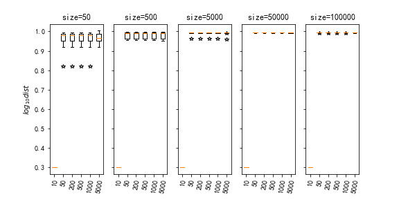
Figure 70: Performance on S395 ($\sigma=1$).

Firstly, we illustrate the algorithm’s performance under a given noise level. The noise level was set to be $\sigma=1.0$. Performance profiles on 12 randomly selected problems was illustrated in Figures 2-12. Each figure includes 5 subfigures corresponding to 5 levels of sample size in $\tilde{S}$. In each subfigure, 6 box plots, each corresponds to a level of iteration labeled in the x-axis, for 20 instances of $\log_{10}\mbox{dist}(x_{k},\mathcal{S}_{opt})$ were drawn. From these figures, we observed that the algorithm’s empirical performance improves with respect to the increase of iteration and sample size; and that the interquartile range decreases significantly when the sample size increases. Figures of the performance on the other 46 problems are contained in Appendix (Fig. 26- Fig.70).

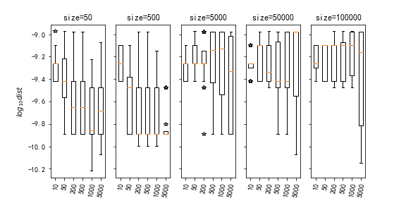
Figure 1: performance on HS11($\sigma=1$).

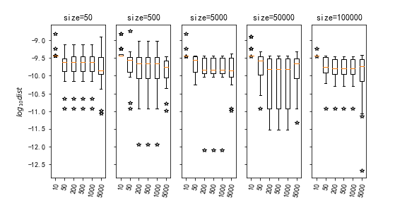
Figure 2: performance on HS20($\sigma=1$).

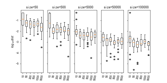
Figure 3: performance on HS30($\sigma=1$).

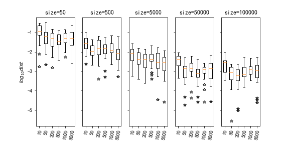
Figure 4: performance on HS31($\sigma=1$).

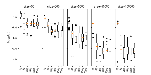
Figure 5: performance on HS46($\sigma=1$).

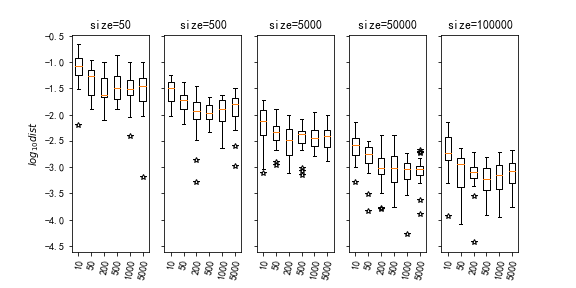
Figure 6: performance on HS60($\sigma=1$).

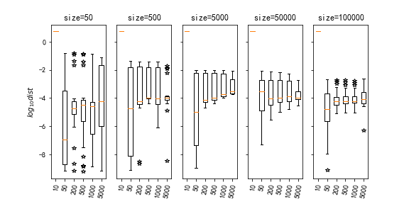
Figure 7: performance on HS61($\sigma=1$).

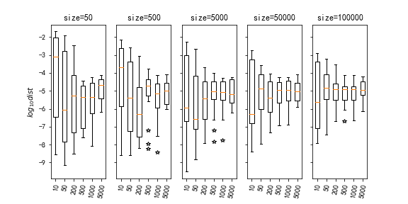
Figure 8: performance on S317($\sigma=1$).

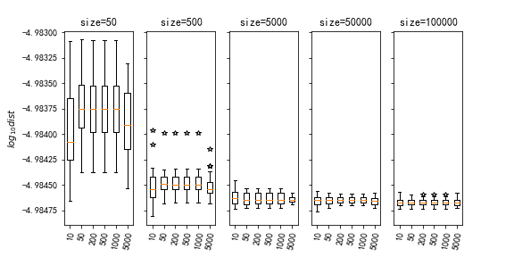
Figure 9: performance on S324($\sigma=1$).

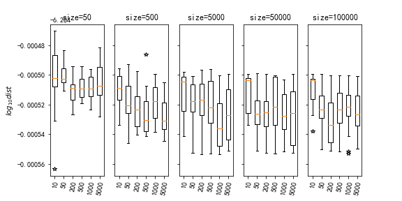
Figure 10: performance on S326($\sigma=1$).

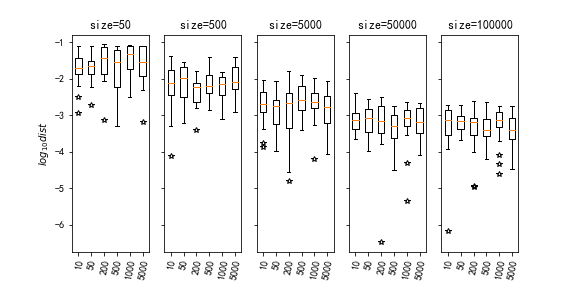
Figure 11: performance on S327($\sigma=1$).

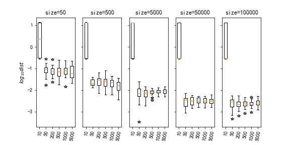
Figure 12: performance on S373($\sigma=1$).

Secondly, we report the variation of the performance of Algorithm 2 with respect to the level of noise. We ran Algorithm 2 on test problems with

$$\sigma\in\{10,1.0,0.1\},$$

and recorded its performance under different cross levels of iteration and sample size. Due to space limitation, we choose two levels of iteration

$$\tilde{K}_{2}=\{500,5000\}$$

and two levels of sample size

$$\tilde{S}_{2}=\{500,100000\}.$$

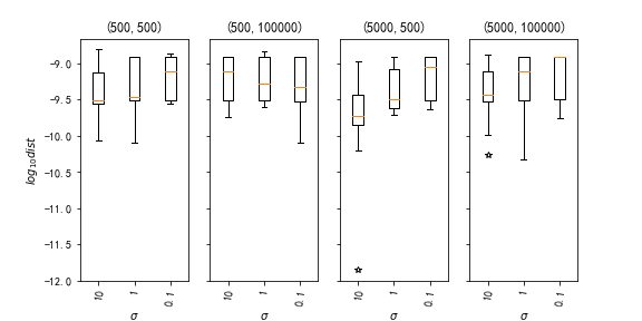
Figure 72: Performance on HS14 w.r.t $\sigma$.

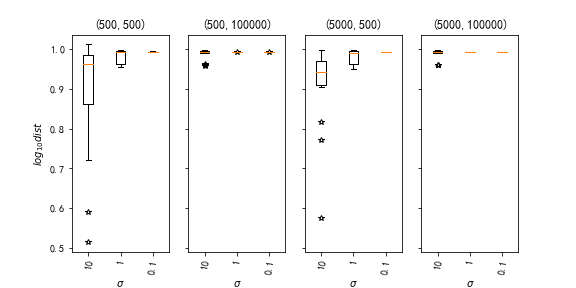
Figure 116: Performance on S395 w.r.t $\sigma$.

Figures 14-24 illustrate the Performance with respect to $\sigma$ on 12 randomly selected problems. All the other figures are included in Appendix (Fig. 72-Fig. 116).

4.4 Observations

We can note several general patterns that can be seen from the figures informative in regards to the specific properties of the Algorithm as well as broad insights for stochastic constrained optimization in general.

From these figures, one can see that Algorithm 2 performs better on instances with small levels of noise, which is to be expected.

In addition, we see that the sample size does affect the noise, but generally speaking not the expectation of the performance. Furthermore, there is often a threshold at which the additional variance reduction is marginal with increasing sample size. This threshold varies depending on the problem.

Finally, we see that as standard with stochastic optimization, there is an exponential increase in the number of iterations required to achieve an order of magnitude. Moreover, there is considerable variation across problems as to how steep this relationship is. This confirms the overall understanding that there is considerable cost in total samples necessary to achieve precision.

This also seems to challenge the overall historical fast local convergence properties of SQP. A careful investigation of sketching and other techniques to maintain this in the stochastic setting could be an important consideration for future work.

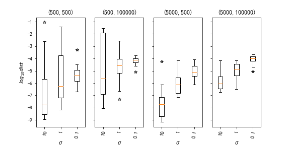
Figure 13: Performance on HS06 w.r.t $\sigma$.

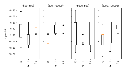
Figure 14: Performance on HS11 w.r.t $\sigma$.

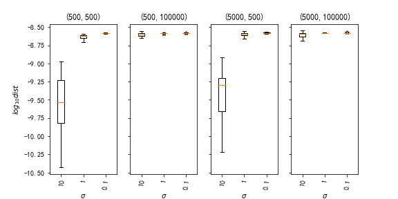
Figure 15: Performance on HS18 w.r.t $\sigma$.

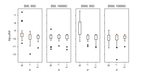
Figure 16: Performance on HS20 w.r.t $\sigma$.

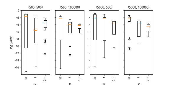
Figure 17: Performance on HS32 w.r.t $\sigma$.

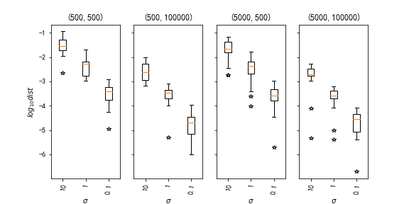
Figure 18: Performance on HS63 w.r.t $\sigma$.

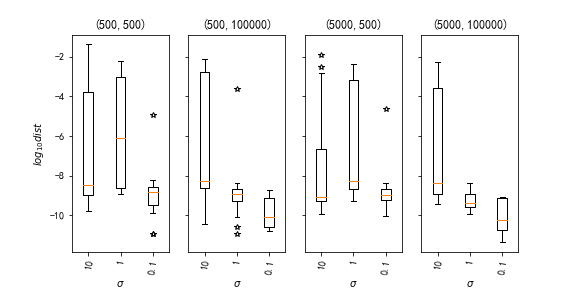
Figure 19: Performance on S216 w.r.t $\sigma$.

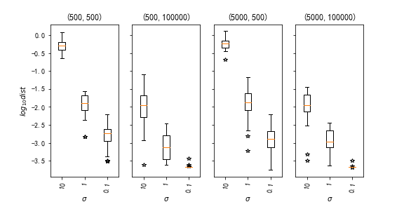
Figure 20: Performance on S252 w.r.t $\sigma$.

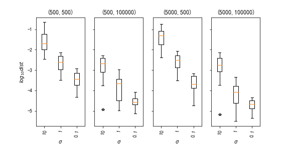
Figure 21: Performance on S316 w.r.t $\sigma$.

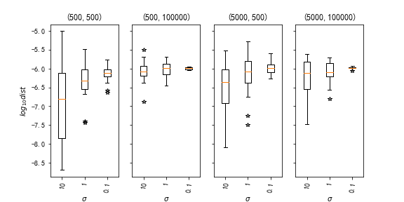
Figure 22: Performance on S322 w.r.t $\sigma$.

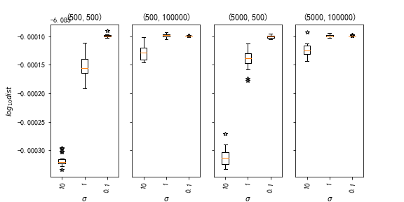
Figure 23: Performance on S323 w.r.t $\sigma$.

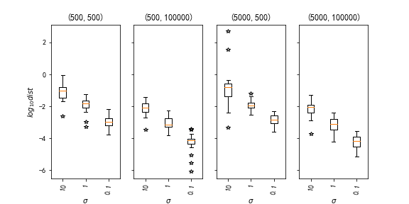
Figure 24: Performance on S337 w.r.t $\sigma$.

5 Conclusions

In this paper, we proposed a robust SQP method for optimization with stochastic objective functions and deterministic constraints. The presented method generalizes Paquette and Scheinberg’s line search method for unconstrained stochastic optimizations to the SQP method for constrained stochastic optimization of the form (1). Ideas of Burke and Han’s robust SQP burke1989robust method are adopted to ensure the consistency of QP subproblems. Global convergence in the case where the penalty parameter is proved, meanwhile the probability of the penalty parameter approaching infinity is shown to be 0, with a specific sampling method. Numerical results on a set of test problems are reported, which illustrate how the performance of the algorithm vary with respect to the number of iterations, the sample size and the levels of noise, providing insight on the method as well as stochastic constrained optimization in general.

Some advanced SQP schemes in deterministic nonlinear programming, for example, the inexact SQP scheme ByrdCN2008 , the filterSQP technique FletcL2002 ; FletcLT2002 , the stabilized SQP scheme Wright1998 and etc, can be used to extend this work. It will be also interesting and deserves studying to exploit other classical schemes for nonlinear constrained optimizations, such as the augmented Lagrangian method and interior point method, to solve stochastic problems. Finally, establishing fast local convergence as well as real time iteration and other online schemes of using SQP, two of the classical strengths of SQP methods, are of interest.

Appendix A Remaining figures of the numerical experiments

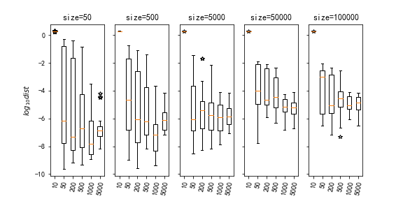
Figure 25: Performance on HS06 ($\sigma=1$).

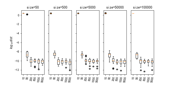
Figure 26: Performance on HS12 ($\sigma=1$).

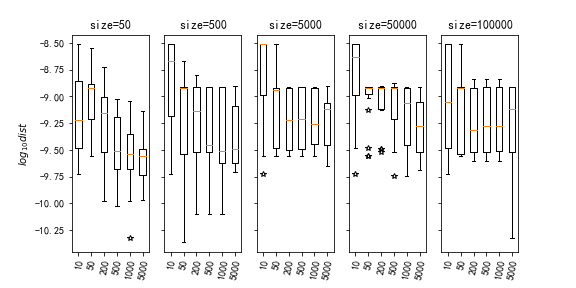
Figure 27: Performance on HS14 ($\sigma=1$).

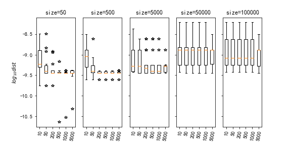
Figure 28: Performance on HS15 ($\sigma=1$).

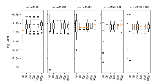
Figure 29: Performance on HS16 ($\sigma=1$).

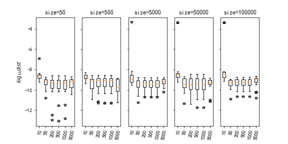
Figure 30: Performance on HS17 ($\sigma=1$).

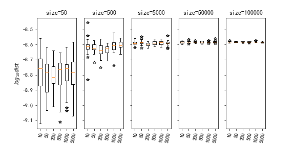
Figure 31: Performance on HS18 ($\sigma=1$).

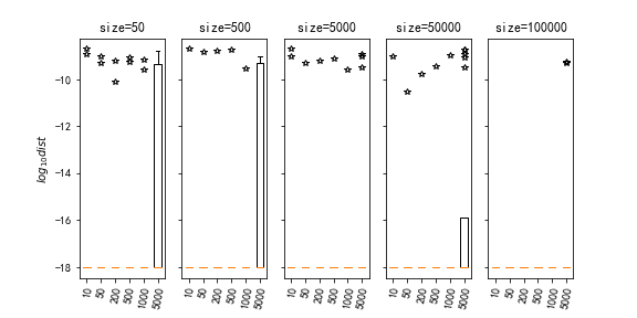
Figure 32: Performance on HS22 ($\sigma=1$).

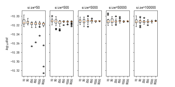
Figure 33: Performance on HS23 ($\sigma=1$).

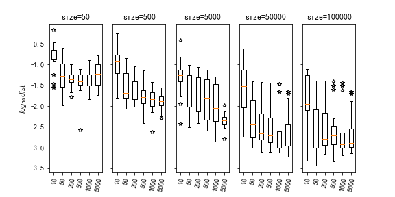
Figure 34: Performance on HS26 ($\sigma=1$).

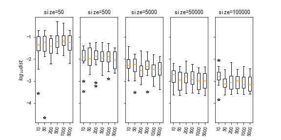
Figure 35: Performance on HS27 ($\sigma=1$).

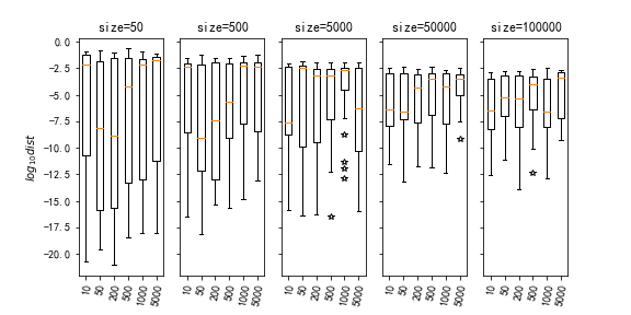
Figure 36: Performance on HS32 ($\sigma=1$).

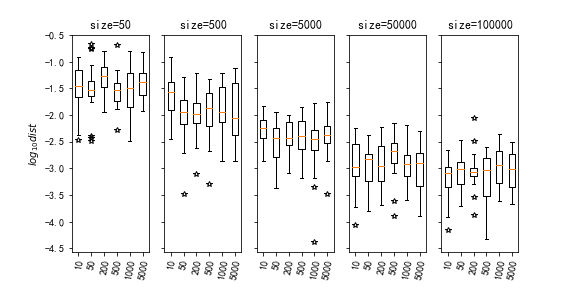
Figure 37: Performance on HS42 ($\sigma=1$).

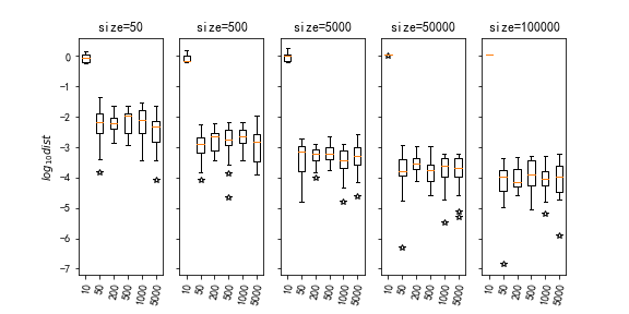
Figure 38: Performance on HS43 ($\sigma=1$).

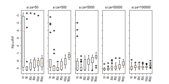
Figure 39: Performance on HS57 ($\sigma=1$).

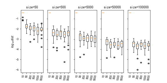
Figure 40: Performance on HS63 ($\sigma=1$).

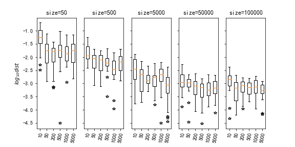
Figure 41: Performance on HS65 ($\sigma=1$).

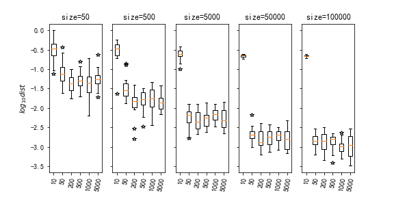
Figure 42: Performance on HS77 ($\sigma=1$).

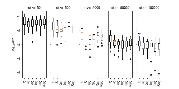
Figure 43: Performance on HS79 ($\sigma=1$).

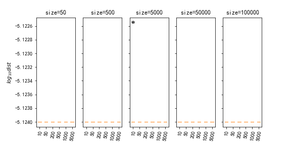
Figure 44: Performance on HS99 ($\sigma=1$).

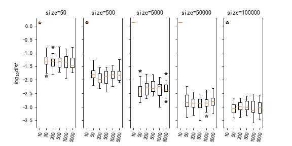
Figure 45: Performance on HS100 ($\sigma=1$).

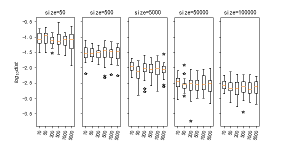
Figure 46: Performance on HS113 ($\sigma=1$).

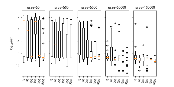
Figure 47: Performance on S216 ($\sigma=1$).

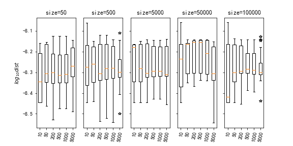
Figure 48: Performance on S225 ($\sigma=1$).

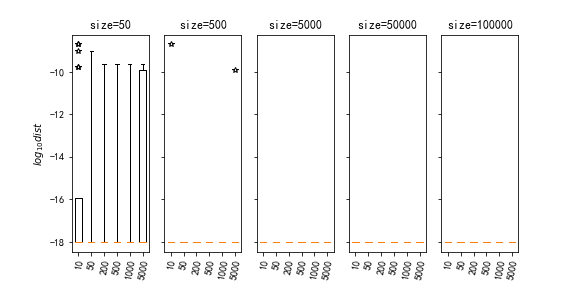
Figure 49: Performance on S227 ($\sigma=1$).

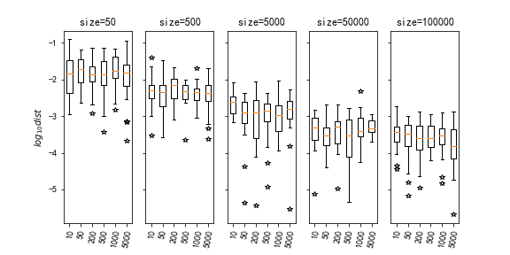
Figure 50: Performance on S233 ($\sigma=1$).

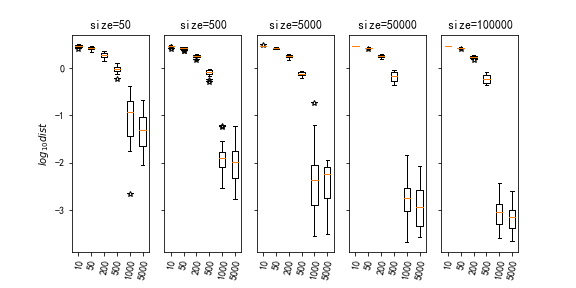
Figure 51: Performance on S235 ($\sigma=1$).

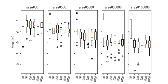
Figure 52: Performance on S249 ($\sigma=1$).

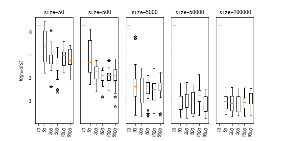
Figure 53: Performance on S252 ($\sigma=1$).

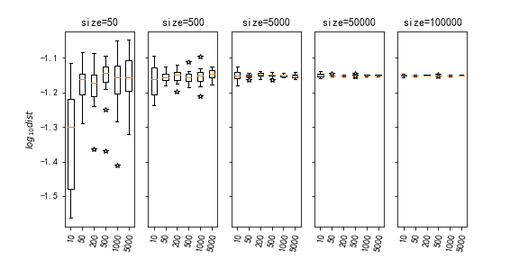
Figure 54: Performance on S264 ($\sigma=1$).

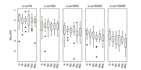
Figure 55: Performance on S316 ($\sigma=1$).

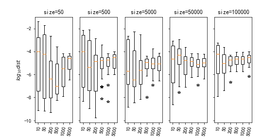
Figure 56: Performance on S318 ($\sigma=1$).

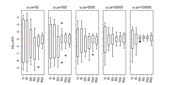
Figure 57: Performance on S319 ($\sigma=1$).

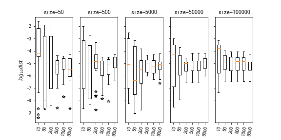
Figure 58: Performance on S320 ($\sigma=1$).

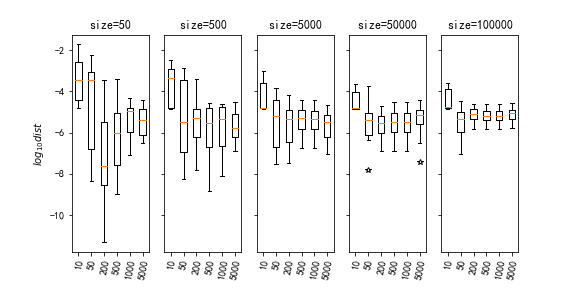
Figure 59: Performance on S321 ($\sigma=1$).

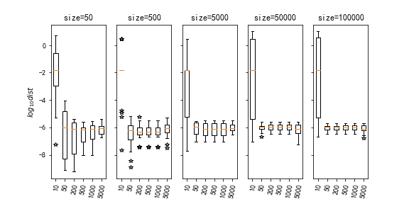
Figure 60: Performance on S322 ($\sigma=1$).

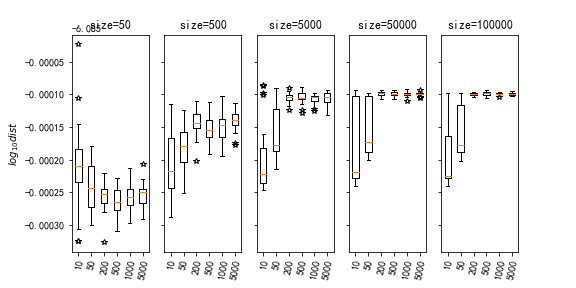
Figure 61: Performance on S323 ($\sigma=1$).

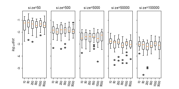
Figure 62: Performance on S337 ($\sigma=1$).

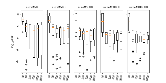
Figure 63: Performance on S338 ($\sigma=1$).

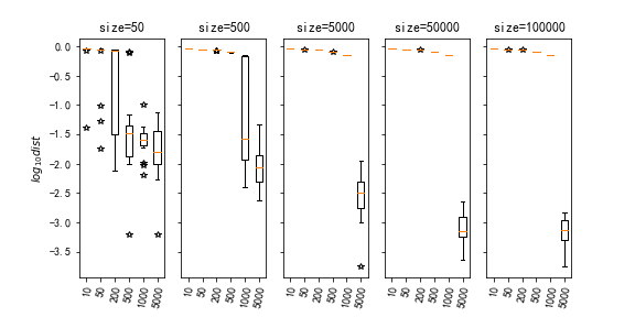
Figure 64: Performance on S344 ($\sigma=1$).

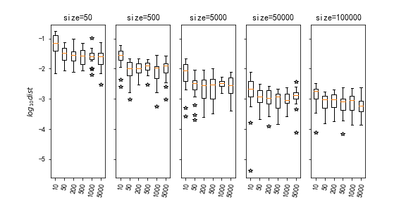
Figure 65: Performance on S345 ($\sigma=1$).

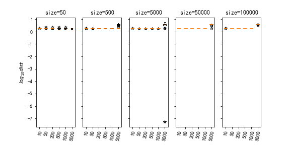
Figure 66: Performance on S355 ($\sigma=1$).

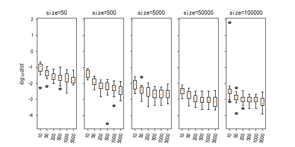
Figure 67: Performance on S372 ($\sigma=1$).

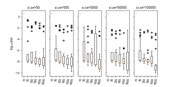
Figure 68: Performance on S375 ($\sigma=1$).

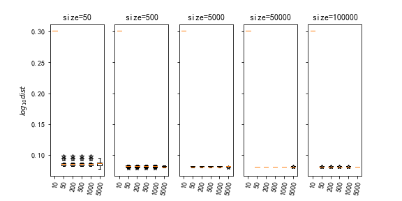
Figure 69: Performance on S394 ($\sigma=1$).

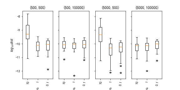
Figure 71: Performance on HS12 w.r.t $\sigma$.

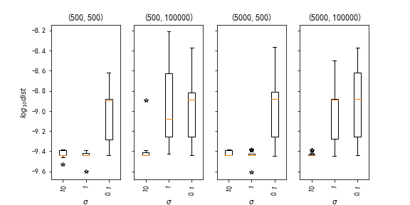
Figure 73: Performance on HS15 w.r.t $\sigma$.

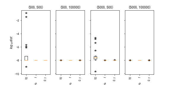
Figure 74: Performance on HS16 w.r.t $\sigma$.

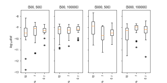
Figure 75: Performance on HS17 w.r.t $\sigma$.

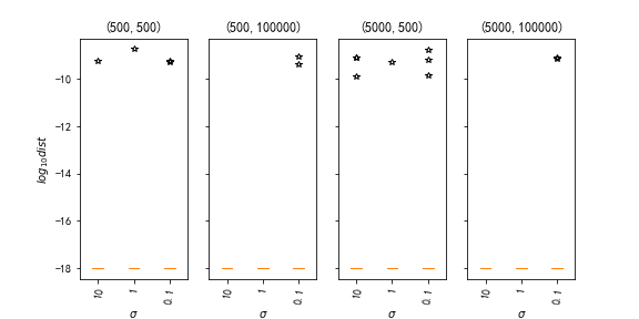
Figure 76: Performance on HS22 w.r.t $\sigma$.

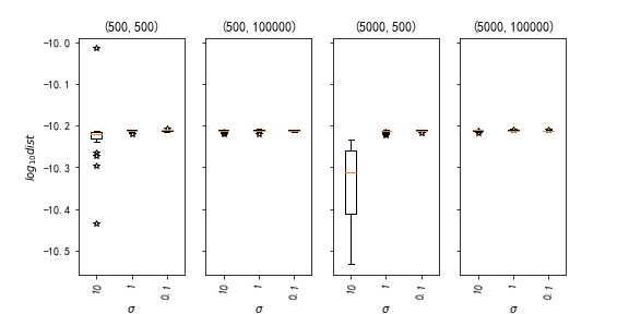
Figure 77: Performance on HS23 w.r.t $\sigma$.

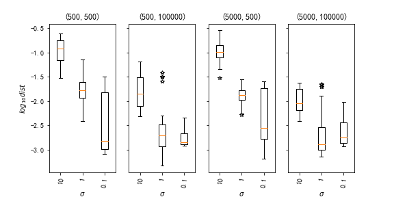
Figure 78: Performance on HS26 w.r.t $\sigma$.

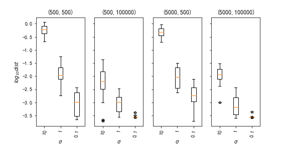
Figure 79: Performance on HS27 w.r.t $\sigma$.

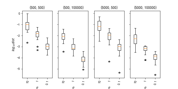
Figure 80: Performance on HS30 w.r.t $\sigma$.

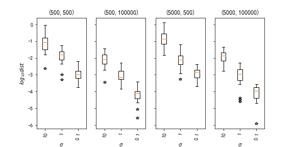
Figure 81: Performance on HS31 w.r.t $\sigma$.

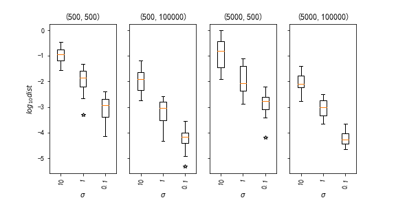
Figure 82: Performance on HS42 w.r.t $\sigma$.

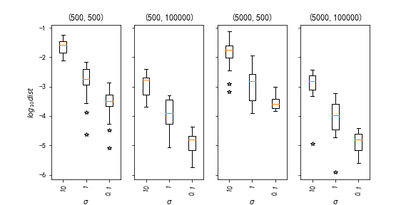
Figure 83: Performance on HS43 w.r.t $\sigma$.

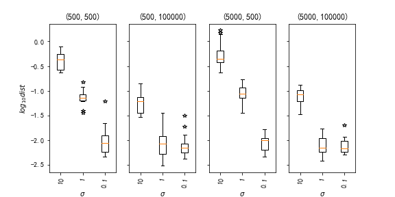
Figure 84: Performance on HS46 w.r.t $\sigma$.

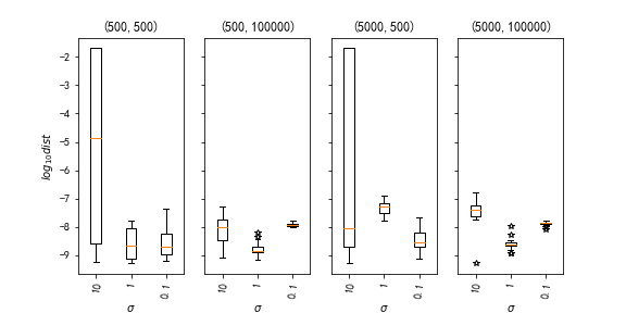
Figure 85: Performance on HS57 w.r.t $\sigma$.

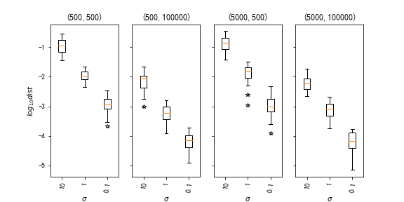
Figure 86: Performance on HS60 w.r.t $\sigma$.

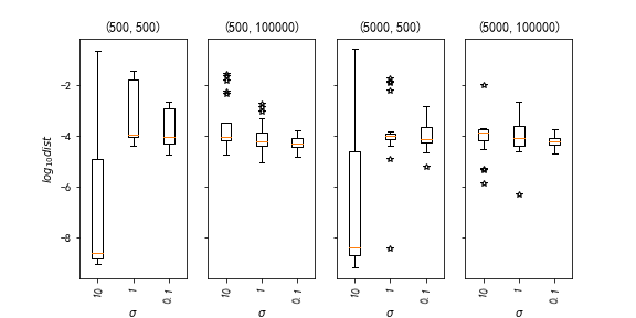
Figure 87: Performance on HS61 w.r.t $\sigma$.

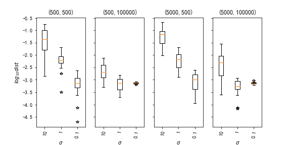
Figure 88: Performance on HS65 w.r.t $\sigma$.

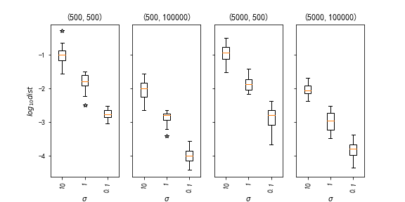
Figure 89: Performance on HS77 w.r.t $\sigma$.

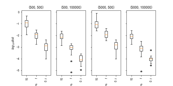
Figure 90: Performance on HS79 w.r.t $\sigma$.

Figure 91: Performance on HS99 w.r.t $\sigma$.

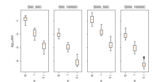
Figure 92: Performance on HS100 w.r.t $\sigma$.

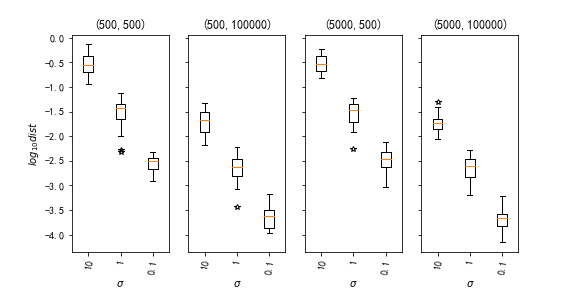
Figure 93: Performance on HS113 w.r.t $\sigma$.

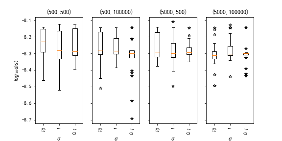
Figure 94: Performance on S225 w.r.t $\sigma$.

Figure 95: Performance on S227 w.r.t $\sigma$.

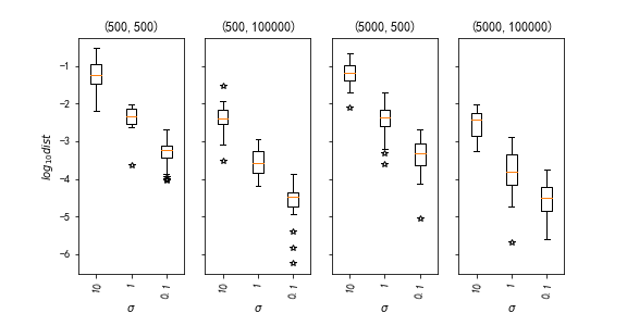
Figure 96: Performance on S233 w.r.t $\sigma$.

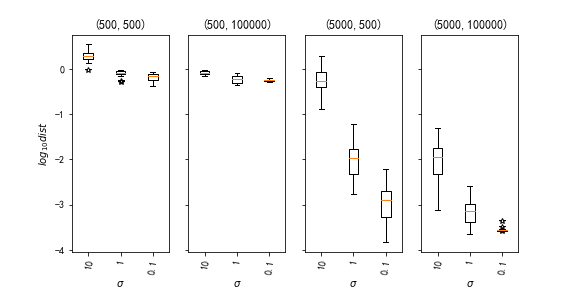
Figure 97: Performance on S235 w.r.t $\sigma$.

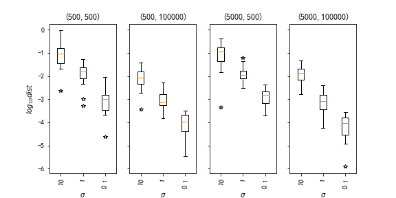
Figure 98: Performance on S249 w.r.t $\sigma$.

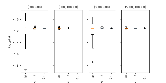
Figure 99: Performance on S264 w.r.t $\sigma$.

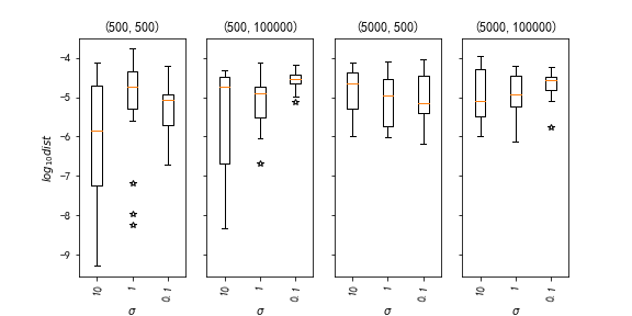
Figure 100: Performance on S317 w.r.t $\sigma$.

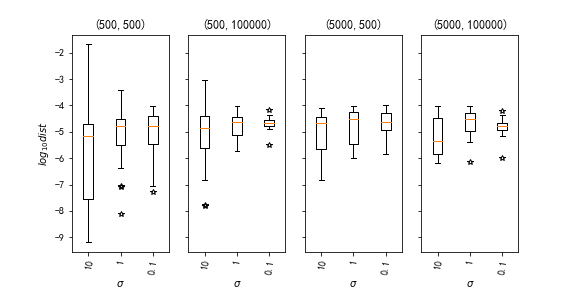
Figure 101: Performance on S318 w.r.t $\sigma$.

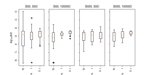
Figure 102: Performance on S319 w.r.t $\sigma$.

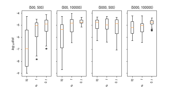
Figure 103: Performance on S320 w.r.t $\sigma$.

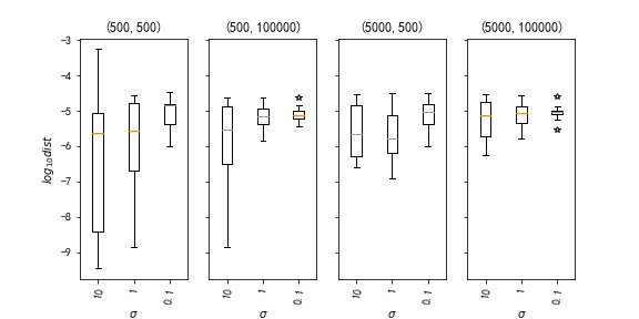
Figure 104: Performance on S321 w.r.t $\sigma$.

Figure 105: Performance on S324 w.r.t $\sigma$.

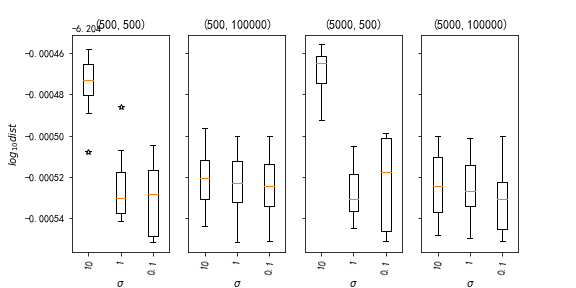
Figure 106: Performance on S326 w.r.t $\sigma$.

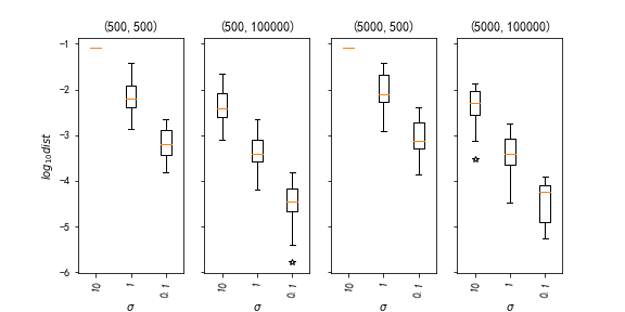
Figure 107: Performance on S327 w.r.t $\sigma$.

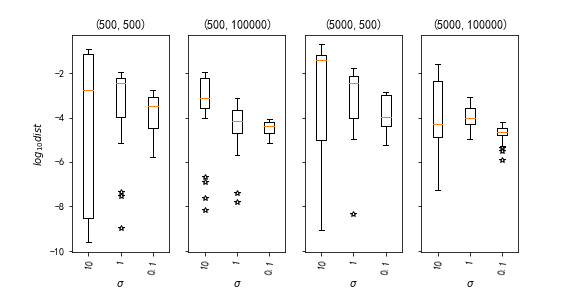
Figure 108: Performance on S338 w.r.t $\sigma$.

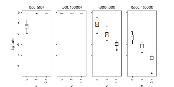
Figure 109: Performance on S344 w.r.t $\sigma$.

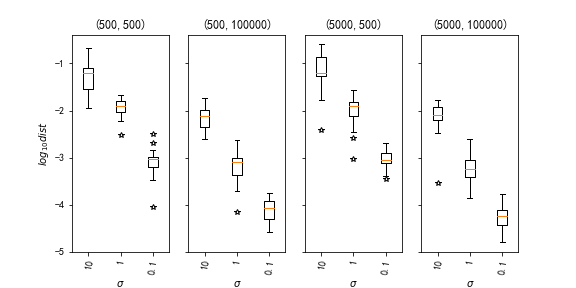
Figure 110: Performance on S345 w.r.t $\sigma$.

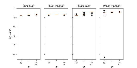
Figure 111: Performance on S355 w.r.t $\sigma$.

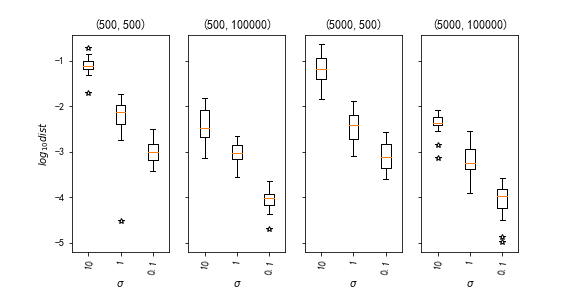
Figure 112: Performance on S372 w.r.t $\sigma$.

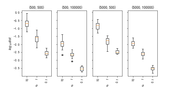
Figure 113: Performance on S373 w.r.t $\sigma$.

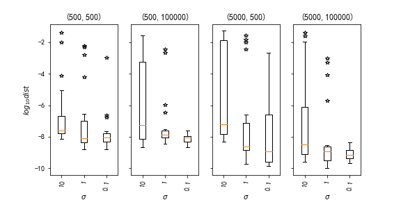
Figure 114: Performance on S375 w.r.t $\sigma$.

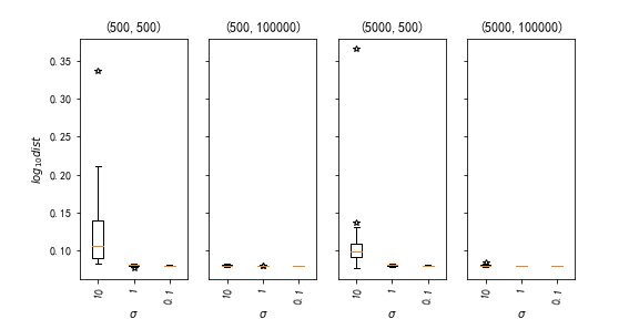
Figure 115: Performance on S394 w.r.t $\sigma$.

References

• \bibcommenthead
• (1) Burke, J.V., Han, S.-P.: A robust sequential quadratic programming method. Mathematical Programming 43(1-3), 277–303 (1989)
• (2) Paquette, C., Scheinberg, K.: A stochastic line search method with expected complexity analysis. SIAM Journal on Optimization 30(1), 349–376 (2020)
• (3) Chen, C., Tung, F., Vedula, N., Mori, G.: Constraint-aware deep neural network compression. In: Ferrari, V., Hebert, M., Sminchisescu, C., Weiss, Y. (eds.) Computer Vision – ECCV 2018, pp. 409–424. Springer, Cham (2018)
• (4) Roy, S.K., Mhammedi, Z., Harandi, M.: Geometry aware constrained optimization techniques for deep learning. In: 2018 IEEE/CVF Conference on Computer Vision and Pattern Recognition, pp. 4460–4469 (2018)
• (5) Nandwani, Y., Pathak, A., Mausam, Singla, P.: A primal-dual formulation for deep learning with constraints. In: Advances in Neural Information Processing Systems 32, pp. 12157–12168 (2019). Curran Associates,Inc.
• (6) Ravi, S.N., Dinh, T., Lokhande, V.S., Singh, V.: Explicitly imposing constraints in deep networks via conditional gradients gives improved generalization and faster convergence. In: Proceedings of the AAAI Conference on Artificial Intelligence, vol. 33, pp. 4772–4779 (2019). Association for the Advancement of Artificial Intelligence (AAAI)
• (7) Kirkegaard, P., Eldrup, M.: POSITRONFIT: A versatile program for analysing positron lifetime spectra. Computer Physics Communications 3(3), 240–255 (1972)
• (8) Kaufman, L., Pereyra, V.: A method for separable nonlinear least squares problems with separable nonlinear equality constraints. SIAM Journal on Numerical Analysis 15(1), 12–20 (1978)
• (9) Nagaraj, N.K., Fuller, W.A.: Estimation of the parameters of linear time series models subject to nonlinear restrictions. The Annals of Statistics 19(3), 1143–1154 (1991)
• (10) Aitchison, J., Silvey, S.D.: Maximum-likelihood estimation of parameters subject to restraints. The Annals of Mathematical Statistics 29(3), 813–828 (1958)
• (11) Silvey, S.D.: The Lagrangian multiplier test. The Annals of Mathematical Statistics 30(2), 389–407 (1959)
• (12) Sen, P.K.: Asymptotic properties of maximum likelihood estimators based on conditional specification. The Annals of Statistics 7(5), 1019–1033 (1979)
• (13) Dupacova, J., Wets, R.: Asymptotic behavior of statistical estimators and of optimal solutions of stochastic optimization problems. The Annals of Statistics 16(4), 1517–1549 (1988)
• (14) Shapiro, A.: On the asymptotics of constrained local $M$-estimators. The Annals of Statistics 28(3), 948–960 (2000)
• (15) Berahas, A.S., Curtis, F.E., Robinson, D., Zhou, B.: Sequential quadratic optimization for nonlinear equality constrained stochastic optimization. SIAM Journal on Optimization 31(2), 1352–1379 (2021)
• (16) Berahas, A.S., Curtis, F.E., O’Neill, M.J., Robinson, D.P.: A Stochastic Sequential Quadratic Optimization Algorithm for Nonlinear Equality Constrained Optimization with Rank-Deficient Jacobians. arXiv (2021). https://doi.org/10.48550/ARXIV.2106.13015
• (17) Curtis, F.E., O’Neill, M.J., Robinson, D.P.: Worst-case complexity of an SQP method for nonlinear equality constrained stochastic optimization. arXiv (2021). https://doi.org/10.48550/ARXIV.2112.14799. https://arxiv.org/abs/2112.14799
• (18) Na, S., Anitescu, M., Kolar, M.: An Adaptive Stochastic Sequential Quadratic Programming with Differentiable Exact Augmented Lagrangians (2021)
• (19) Berahas, A.S., Shi, J., Yi, Z., Zhou, B.: Accelerating stochastic sequential quadratic programming for equality constrained optimization using predictive variance reduction. arXiv (2022). https://doi.org/10.48550/ARXIV.2204.04161. https://arxiv.org/abs/2204.04161
• (20) Na, S., Anitescu, M., Kolar, M.: Inequality constrained stochastic nonlinear optimization via active-set sequential quadratic programming. arXiv (2021). https://doi.org/10.48550/ARXIV.2109.11502. https://arxiv.org/abs/2109.11502
• (21) Blanchet, J., Cartis, C., Menickelly, M., Scheinberg, K.: Convergence rate analysis of a stochastic trust-region method via supermartingales. INFORMS Journal on Optimization 1(2), 92–119 (2019)
• (22) Burke, J., Han, S.-P.: A Gauss-Newton approach to solving generalized inequalites. Mathematics of Operations Research 11(4), 632–643 (1986)
• (23) Powell, M.J.D.: A fast algorithm for nonlinearly constrained optimization calculations. In: Watson, G.A. (ed.) Numerical Analysis. Lecture Notes in Mathematics, vol. 630, pp. 144–157. Springer, Berlin Heidelberg (1978)
• (24) Byrd, R.H.: Robust trust region methods for constrained optimization. In: Third SIAM Conference on Optimization (1987)
• (25) Omojokun, E.: Trust region algorithm for optimization with equalities and inequalities constraints. PhD thesis, University of Cororado at Boulder (1989)
• (26) Fletcher, R., Leyffer, S.: Nonlinear programming without a penalty function. Mathematical Programming 91(2), 239–269 (2002)
• (27) Fletcher, R., Leyffer, S., Toint, P.: On the global convergence of a filter–SQP algorithm. SIAM Journal on Optimization 13(1), 44–59 (2002)
• (28) Curtis, F.E., Nocedal, J., Wächter, A.: A matrix-free algorithm for equality constrained optimization problems with rank-deficient jacobians. SIAM Journal on Optimization. 20(3), 1224–1249 (2009)
• (29) Dennis, J.E., El-Alem, M., Maciel, M.C.: A global convergence theory for general trust-region-based algorithms for equality constrained optimization. SIAM Journal on Optimization 7(1), 177–207 (1997)
• (30) Fletcher, R., Gould, N.I., Leyffer, S., Toint, P.L., Wächter, A.: Global convergence of a trust-region SQP-filter algorithm for general nonlinear programming. SIAM Journal on Optimization. 13(3), 635–659 (2002)
• (31) Bertsekas, D.P.: Nonlinear Programming, 3rd edn. Athena Scientific, Belmont, Massachusetts (2016)
• (32) Gauvin, J.: A necessary and sufficient regularity condition to have bounded multipliers in nonconvex programming. Mathematical Programming 12(1), 136–138 (1977)
• (33) Cartis, C., Scheinberg, K.: Global convergence rate analysis of unconstrained optimization methods based on probabilistic models. Mathematical Programming 169(2), 337–375 (2018)
• (34) Nocedal, J., Wright, S.J.: Numerical Optimization, 2nd edn. Springer, New York (2006)
• (35) Robinson, S.M.: A characterization of stability in linear programming. Operations Research 25(3), 435 (1977)
• (36) Cánovas, M.J., López, M.A., Parra, J., Toledo, F.J.: Lipschitz continuity of the optimal value via bounds on the optimal set in linear semi-infinite optimization. Mathematics of Operations Research 31(3), 478–489 (2006)
• (37) Schaeffer, D.G., Cain, J.W.: Ordinary Differential Equations: Basics and Beyond, 1st edn. Texts in Applied Math. Springer, New York, NY (2016)
• (38) Di Pillo, G., Grippo, L.: On the exactness of a class of nondifferentiable penalty functions. Journal of Optimization Theory and Applications 57(3), 399–410 (1988)
• (39) Di Pillo, G., Grippo, L.: Exact penalty functions in constrained optimization. SIAM Journal on Control and Optimization 27(6), 1333–1360 (1989)
• (40) Sun, W., Yuan, Y.-X.: Optimization Theroy and Methods. Springer Optimization and Its Applications. Springer, Boston, MA (2006)
• (41) Klenke, A.: Probability Theory: a Comprehensive Course. Springer, ??? (2013)
• (42) Hock, W., Schittkowski, K.: Test examples for nonlinear programming code. In: Lecture Notes in Economics and Mathematical Systems vol. 187. Springer, Berlin (1981)
• (43) Schittkowski, K.: More test examples for nonlinear programming codes. In: Lecture Notes in Economics and Mathematical Systems. Springer, Berlin (1987)
• (44) Byrd, R., Curtis, F., Nocedal, J.: An inexact SQP method for equality constrained optimization. SIAM Journal on Optimization. 19(1), 351–369 (2008). https://doi.org/10.1137/060674004
• (45) Wright, S.J.: Superlinear convergence of a stabilized SQP method to a degenerate solution. Computational Optimization and Applications 11(3), 253–275 (1998)