s s m m m #1 #2 ⟨#3—#4—#5⟩ #3#4#5⟨#3—#4—#5⟩ #4⟨#3—#4—#5⟩

Phase transition in Stabilizer Entropy and efficient purity estimation

Abstract

Stabilizer Entropy (SE) quantifies the spread of a state in the basis of Pauli operators. It is a computationally tractable measure of non-stabilizerness and thus a useful resource for quantum computation. SE can be moved around a quantum system, effectively purifying a subsystem from its complex features. We show that there is a phase transition in the residual subsystem SE as a function of the density of non-Clifford resources. This phase transition has important operational consequences: it marks the onset of a subsystem purity estimation protocol that requires $\operatorname{poly}(n)\exp(t)$ many queries to a circuit containing $t$ non-Clifford gates that prepares the state from a stabilizer state. Then, for $t=O(\log n)$, it estimates the purity with polynomial resources and, for highly entangled states, attains an exponential speed-up over the known state-of-the-art algorithms.

Introduction.— Quantum information processing promises an advantage over its classical counterpart [1, 2, 3, 4, 5, 6, 7]. Since the inception of this field [8], there has been an extensive theoretical investigation as to what ingredients do quantum computation possesses such that it is intrinsically computationally more powerful than classical computation.

The two resources that set quantum computers apart are entanglement [9, 10, 11, 12] and non-stabilizerness [8, 13]. Without either of them, quantum computers cannot perform any advantageous algorithm over classical devices [1, 2, 14]. In particular, non-stabilizerness measures how many universal gates one can distill from a given quantum state [15, 16, 17, 18, 19] and the cost of simulating a quantum state on a classical computer. Indeed, while stabilizer states – the orbit of the Clifford group [20] – can be simulated classically in polynomial time [8], the cost of the simulation scales exponentially in the number of non-stabilizer resources [21, 22], i.e. unitary gates outside the Clifford group [8].

At the same time, many information processing tasks in quantum computing become inefficient exactly because of the conspiracy of entanglement and nonstabilizerness. Examples of this kind are: state certification [23], disentangling [24, 25, 26, 27, 28, 29] or unscrambling [31, 32, 33]. In particular, while purity estimation is a resource-intensive task for universal states, it can be achieved efficiently for stabilizer states.

It seems then that quantum computation is plagued by a catch-22: on the one hand, stabilizer information can be efficiently processed but for the same reason it is useless for a fruitful quantum computation. On the other hand, the combination of entanglement and nonstabilizerness, which makes quantum technology powerful, hinders the efficiency of measurement tasks. Given that, the question posed by this paper is the following: can we leverage the efficiency of information processing offered by the stabilizer formalism for non-stabilizer states?

Recently, a novel measure of non-stabilizerness has been introduced as stabilizer entropy (SE) [34]. Stabilizer states have zero stabilizer entropy, whereas non-stabilizer states – those that are computationally useful – exhibit a non-vanishing stabilizer entropy. Unlike other measures [15, 35, 36], it is computable (though expensive) and experimentally measurable [37, 38, 39]. SE is also involved in the onset of universal, complex patterns of entanglement [29, 28], quantum chaos [40, 41, 42, 43], complexity in the wave-function of quantum many-body systems [44, 45], and the decoding algorithms from the Hawking radiation from old black holes [31, 33, 32]. In the context of operator spreading, it is akin to the string entropy [30].

As we said, when states possess SE, measurement tasks tend to become inefficient. However, the intriguing aspect of entropy is that it can be transferred from one subsystem to another without altering the total entropy, and thus the total computational power of the system. This parallels the behavior of a Carnot refrigerator that effectively reduces entropy in a system by transferring it to the environment, all while keeping the entropy of the universe unchanged.

In this paper, drawing inspiration from this thermodynamic analogy, we show a general scheme of how to push SE out of a subsystem with Clifford operations – effectively cooling the subsystem down from its complex features while preserving the total SE – and explore the consequences and implications of this approach. The two main results of this paper are the following:

(i) There is a phase transition in SE driven by the competition between the creation and spreading of non-Clifford resources versus their localization and erasure.

(ii) The localized phase – when a subsystem is successfully cleansed of its nonstabilizerness quantified by SE – allows for a purity estimation algorithm that, for some cases of interest, obtains an exponential speed-up over all the state-of-the-art known algorithms [46, 47, 48, 49, 50, 51, 52]. In practice, this result is obtained by constructing a stabilizer state whose subsystem purity is shown to bound the purity of the desired state.

Setup.— Consider a system of $n$ qubits with Hilbert space $\mathcal{H}\simeq{\rm\kern 2.40005pt\vrule width=0.39993pt,height=6.28612pt,depth=-0.3014pt\kern-2.89993ptC}^{\otimes 2n}\simeq\mathcal{H}_{E}\otimes\mathcal{H}_{F}$ with dimensions $d_{X}=2^{n_{X}}$ with $(X=E,F)$ and $n=n_{E}+n_{F}$. Let $|\mathbf{0}\rangle\equiv|0\rangle^{\otimes n}$. To every pure density operator $\psi$ on $\mathcal{H}$ one can associate a probability distribution $P_{\psi}$ through its decomposition $\psi=d^{-1}\sum_{P\in\mathbb{p}}\mathrm{tr}(P\psi)P$ in Pauli operators $P\in\mathbb{P}$ by $P_{\psi}=d^{-1}\mathrm{tr}^{2}(P\psi)$. Regardless of the purity of $\psi$, its stabilizer purity is defined as $\mbox{SP}(\psi):=\sum_{P}P_{\psi}^{2}$. On the other hand, the purity of the state $\psi$ is given by $\operatorname{Pur}(\psi)=\mathrm{tr}(\psi^{2})$. Defining the ratio $w(\psi):=d\,\mbox{SP}(\psi)/\operatorname{Pur}(\psi)$, the $2-$Rényi SE is given by $M(\psi)=-\log w$ [34], while the linear SE is defined as $M_{\operatorname{lin}}=1-w$. Throughout the paper, we define stabilizer states those for which $M(\psi)=0$.

Through standard techniques one can write these purities as $\mbox{SP}(\psi)=d\mathrm{tr}(Q\psi^{\otimes 4})$ and $\operatorname{Pur}(\psi)=\mathrm{tr}(T\psi^{\otimes 2})$ where $T$ is the swap operator and $Q=d^{-2}\sum_{P}P^{\otimes 4}$ is the projector onto the stabilizer code [20]. Given the bipartition $E|F$ defined above, one can define the SE associated to the subsystem $X$ as $M_{X}(\psi)\equiv M(\psi_{X})$ where the partial states are defined as $\psi_{E}\equiv\mathrm{tr}_{F}\psi$ and $\psi_{F}\equiv\mathrm{tr}_{E}\psi$. In terms of the $Q,T$ operators the $w$ of the partial state reads $w(\psi_{X})=d_{X}\mathrm{tr}(Q_{X}\psi^{\otimes 4})/\mathrm{tr}(T_{X}\psi^{\otimes 2})$ where now $Q_{X},T_{X}$ are the $Q$ and swap operator on the subsystem $X=E,F$. Note also that if $\psi$ is a stabilizer state then $M_{X}(\psi)=0$ for every subsystem $X$ [34]. However, whether the partial trace is in general a SE-non-increasing map is an open question.

In the following, we are interested in the SE of states $\psi_{t}$ parametrised by a number $t$ of non-Clifford resources. To this end, we consider outputs $\psi_{t}\equiv C_{t}|\mathbf{0}\rangle\!\langle\mathbf{0}|C_{t}^{{\dagger}}$ of $t-$doped Clifford circuits $C_{t}$, that is, Clifford circuits in which have been injected $t$ non-Clifford gates, say $T-$gates [27, 42]. Now, since the Clifford group is very efficient in entangling, the states $\psi_{t}$ are typically highly entangled [24, 26, 20, 54]. As a result, if $n_{F}\ll n_{E}$, the partial state $\psi_{tF}$ is very close to the maximally mixed state, which is a stabilizer state with SE equal zero. We can indeed show that the average $\mathbb{E}_{C}$ (over the Clifford group) SE in $F$ is very small while it is all contained in the subsystem $E$ (see [55]):

Proposition 1. Let $\psi$ a pure state and denote $\psi^{C}\equiv C\psi C^{{\dagger}}$, for $C$ a Clifford circuit. The average over the Clifford orbit of the partial SEs of subsystems $E,F$ is given by

$$\mathbb{E}_{C}[M_{\operatorname{lin}}(\psi^{C}_{E})] = M_{\operatorname{lin}}(\psi)+O\left(\frac{d_{F}}{d_{E}}\right)$$

$$\mathbb{E}_{C}[M_{\operatorname{lin}}(\psi^{C}_{F})] = O\left(\frac{d_{F}}{d_{E}}\right)$$

for large $n$. In the manuscript, we frequently make use of the big-O notation, see [55] for a brief review.

The above formulae show how the SE is all in the larger system. As a corollary, on average over the Clifford orbit of $\psi$, the partial trace preserves SE in the sense that $M(\psi)\simeq M_{E}(\psi)+M_{F}(\psi)$.

Cleansing algorithm.— As we have seen, typically all the SE is contained in the greater of the two subsystems, namely the subsystem $E$. As such, quantum information contained in the state $\psi_{E}$ cannot be efficiently processed [21]: it contains almost all of the quantum complexity induced by the circuit $C_{t}$. One asks whether it is possible to cleanse $E$ from this complexity. If one could do that, one would be able to manipulate $E$ efficiently by means of the stabilizer formalism [56]. Since the SE is an entropy, one wonders if one could toss it in the other subsystem $F$ by means of a suitable protocol. Here, we set the problem up in the following way: can we find a quantum map $\mathcal{E}(\cdot):=\mathrm{tr}_{Y}W(\cdot)W^{\dagger}$ with $W$ a Clifford unitary and $Y$ a subset of $n_{Y}$ qubits $Y\subseteq F$, such that $M_{E}(\mathcal{E}(\psi_{t}))=0$?

To this end, we utilize a fundamental result obtained in [32]: given a $t-$doped circuit $C_{t}$ the so-called Clifford Completion algorithm can learn - by $\operatorname{poly}(n)\exp(t)$ query accesses to a unknown $C_{t}$ - a Clifford operator ${D}$ called diagonalizer such that $C_{t}={D}^{{\dagger}}c_{t}{D}V$, where $c_{t}$ is a $t-$doped Clifford circuit acting on a subsystem with only $t$ qubits (for $t\leq n$) and $V$ is another suitable Clifford unitary operator. This result ensures that $t=O(\log n)$ the operator $D$ will (with negligibly small failure probability) be found in polynomial time.

Now, consider the permutation operator $T_{\pi}$ on $n$ qubits, namely $T_{\pi}|x\rangle=|\pi(x)\rangle$ with $\pi\in S_{n}$ the symmetric group of $n$ objects. Note that the $T_{\pi}$’s also belong to the Clifford group. Then, one can choose a suitable permutation $\pi_{Y}$ such that the dressed operator $T_{\pi_{Y}}c_{t}T_{\pi_{Y}}^{{\dagger}}\equiv c_{t}^{Y}$ acts non trivially only on any desired subsystem $Y\subset E\cup F$, where $n_{Y}=t$. In particular, one can choose $Y\subset F$ if $n_{Y}\leq n_{F}$. As a result, one has $T_{\pi_{Y}}D|\psi_{t}\rangle=T_{\pi_{Y}}c_{t}T_{\pi_{Y}}^{{\dagger}}|\Phi\rangle=c_{t}^{Y}|\Phi\rangle$ with $|\Phi\rangle:=T_{\pi_{Y}}DV|\mathbf{0}\rangle$ being a stabilizer state (with density operator $\Phi\equiv|\Phi\rangle\!\langle\Phi|$). Then, by picking $W\equiv T_{\pi_{Y}}D$, we define the Clifford map $\mathcal{E}(\cdot):=\mathrm{tr}_{Y}W(\cdot)W^{{\dagger}}$ that first localizes the non-Clifford resources in $Y$ and then erases them by tracing $Y$ out. We can now prove the following.

Proposition 2. For $n_{Y}\leq n_{F}$, the map $\mathcal{E}$ moves the $t$ non-Clifford gates in the subsystem $Y\subset F$, and by tracing out $Y$ makes the SE on $E$ zero, i.e. $M_{E}(\mathcal{E}(\psi_{t}))=0$.

Proof.— Start with

$$M_{E}(\mathcal{E}(\psi_{t}))=-\log d_{E}\frac{\mathrm{tr}(Q_{E}\mathcal{E}(\psi_{t})^{\otimes 4})}{\mathrm{tr}(T_{E}\mathcal{E}(\psi_{t})^{\otimes 2})}$$

and recall that $\mathcal{E}(\psi_{t})=\mathrm{tr}_{Y}(c^{Y}_{t}\Phi c^{Y{\dagger}}_{t})$. Now, since $[c_{t}^{Y\otimes 4},Q_{E}]=[c_{t}^{Y\otimes 2},T_{E}]=0$, one obtains $\mathrm{tr}(Q_{E}\mathcal{E}(\psi_{t})^{\otimes 4})=\mathrm{tr}_{E}(Q_{E}\Phi_{E}^{\otimes 4})$ and $\mathrm{tr}(T_{E}\mathcal{E}(\psi_{t})^{\otimes 2})=\mathrm{tr}_{E}(T_{E}\Phi_{E}^{\otimes 2})$ from which one gets $M_{E}(\mathcal{E}(\psi_{t}))=M_{E}(\Phi)=0$, where the last equality follows from $\Phi$ being a stabilizer state [34]. ∎

Phase transition in SE.— We now show that doped Clifford circuits feature a phase transition in SE due to the competition between a term that creates and spreads SE and a term that localizes and then erases it. The first term is the quantum circuit $C_{t}$. As we have seen in the previous section, this unitary operator can be written as $C_{t}=D^{{\dagger}}c_{t}DV$. The unitary $c_{t}$ does insert a number $t$ of non-Clifford gates in a $t$-qubits subsystem, and then the term $D$ spreads them around the whole system. In the large $n$ limit, we can define $\mathfrak{t}:=t/n$ the density of non-Clifford gates and $\mathcal{C}_{\mathfrak{t}}$ its adjoint action. The spreading strength of this channel is given by the depth of $C_{t}$, while its SE strength is given by the density $\mathfrak{t}$. The map $\mathcal{E}$, on the other hand, first localizes the SE in the subsystem $Y\subset F$ and then erases it by entangling and tracing out. Thanks to Proposition $2$, its localizing strength is given by the density of qubits belonging to $F$, namely $\mathfrak{f}:=n_{F}/n$. Altogether, we consider the map composing the two terms, namely $\mathcal{E}\circ\mathcal{C}_{\mathfrak{t}}$ and study the behavior of the SE induced by such a map. In the limit of $\mathfrak{t}/\mathfrak{f}\ll 1$, we expect the map to leave the subsystem $E$ clear of SE. On the other hand, for $\mathfrak{t}/\mathfrak{f}\gg 1$, all the SE should be intact in $E$.

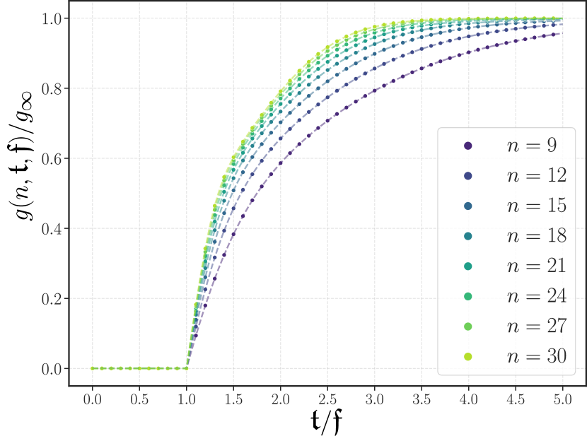
Figure 1: Plot of the ratio between $g(n,\mathfrak{t},\mathfrak{f})$ and $g_{\infty}$, which is a lower bound for the localized SE power of the map $\mathcal{E}\circ\mathcal{C}_{\mathfrak{t}}$, as a function of the ratio of the density $\mathfrak{t}$ of non-Clifford gates to the density $\mathfrak{f}$ of qubits belonging to $F$. We set $\mathfrak{f}=\frac{1}{3}$. The critical point for the phase transition is $\mathfrak{t}/\mathfrak{f}=1$, with critical index one.

We compute the localizing SE power of the map $\mathcal{E}\circ\mathcal{C}_{\mathfrak{t}}$ by averaging the value of $M_{E}(\mathcal{E}\circ\mathcal{C}_{\mathfrak{t}}(\omega))$ over all the maps $\mathcal{E}\circ\mathcal{C}_{\mathfrak{t}}$ and all the (pure) stabilizer input states $\omega$. We denote such an average $\mathbb{E}$ (see [55]). For $\mathfrak{t}/\mathfrak{f}\leq 1$ we obtain, in virtue of Proposition 2, $\mathbb{E}\,\left[M_{E}(\mathcal{E}\circ\mathcal{C}_{\mathfrak{t}}[\omega])\right]=0$. This is the localized phase, where the localizing power of the map $\mathcal{E}$ prevails. On the other hand, for $\mathfrak{t}/\mathfrak{f}\geq 1$, direct computation of the average yields, in the delocalized phase,

$$\mathbb{E}[M_{E}(\mathcal{E}\circ\mathcal{C}_{\mathfrak{t}}[\omega])]\geq g(n,\mathfrak{t},\mathfrak{f})$$ (1)

See [55] for details and the explicit expression for $g(n,\mathfrak{t},\mathfrak{f})$. For large $n$, one has

$$g_{\infty}\equiv\lim_{t\rightarrow\infty}g(n,\mathfrak{t},\mathfrak{f})\simeq n(1-2\mathfrak{f})$$ (2)

In Fig. 1, we plot $g(n,\mathfrak{t},\mathfrak{f})/g_{\infty}$ (for $\mathfrak{f}=1/3$). In the neighborhood of the critical value $\mathfrak{t}/\mathfrak{f}=1$ this ratio behaves as $g(n,\mathfrak{t},\mathfrak{f})/g_{\infty}\simeq\frac{\mathfrak{f}}{1-\mathfrak{f}}\left(\mathfrak{t}/\mathfrak{f}-1\right)$, which shows a critical index one, see Fig. 1.

Efficient purity estimation.— The phase transition described above has relevant operational applications in terms of quantum information processing. We have seen that in the localized phase $\mathfrak{t}/\mathfrak{f}\leq 1$, the SE can be cleansed from the subsystem $E$, making the subsystem $E$ manipulable by means of the stabilizer formalism. We now show that in this phase it is possible to probe the bipartite entanglement in a way that, for cases of interest, gains an exponential speed-up over the state-of-the-art algorithms in the literature [46, 52].

The best-known way to evaluate the purity of a quantum state within an error $\epsilon$ is the swap test, which requires a number of resources scaling as $O(\epsilon^{-2})$. However, typical states possess a subsystem purity $\Theta(e^{-\tilde{\beta}n_{F}})$, the so-called volume law scenario. In this case, to evaluate the purity, one needs to resolve an exponentially small error and therefore exponential (in $n_{F}$ ) resources, which, since $n_{F}=\mathfrak{f}n$, is $\Theta(e^{2{\beta}n})$, with $\beta\equiv\tilde{\beta}\mathfrak{f}$.

If the purity one wants to estimate scales polynomially, that is, $\operatorname{Pur}(\psi_{E})=\Omega(\mbox{poly}^{-1}(n))$, one will need a polynomial number $N_{shot}$ of measurements in order to resolve the quantity. Notice that one would not know beforehand what is the number $N_{shot}$ necessary. In practice, one sets a number of experiments $N_{shot}$ to obtain upper bound thresholds $\operatorname{Pur}(\psi_{E})\leq O(N_{shot}^{-1/2})$. If $\mbox{poly}(n)$ is a large polynomial, one would in practice be forced to halt the procedure without knowing how tight the bound is. In the worst-case scenario (which is also typical), the purity to evaluate is exponentially small and the estimation will always be exponentially costly.

We want to show that the cleansing algorithm can give an exponential advantage over the known protocols. The intuition is that if one can cleanse the SE from $\psi_{E}$, one would obtain a stabilizer state, whose purity can be evaluated with polynomial resources [58].

Let us start with some technical preliminaries. Consider a state initialized in $|\mathbf{0}\rangle$ and be $|\psi_{t}\rangle=C_{t}|\mathbf{0}\rangle$ the output of a $t-$doped Clifford circuit. Its marginal state to $E$ will be denoted by $\psi_{E}=\mathrm{tr}_{F}(\psi_{t})$. This is the state whose purity we want to evaluate. In the localized phase of the cleansing algorithm, we know that the output state $\mathcal{E}(\psi_{t})$ is a stabilizer state of $E\cup F\setminus Y$ for $Y\subset F$. Its purity would be easy to evaluate, but it is not directly related to the purity of the original state $\psi_{E}$ because of the action of $W$. We now show that we can manipulate the cleansed state $\mathcal{E}(\psi_{t})$ and construct a stabilizer state $\rho$ whose purity bounds the purity of the desired state $\psi_{E}$.

Starting from the cleansed state $\mathcal{E}(\psi_{t})$, we first append the maximally mixed state $d_{Y}^{-1}I_{Y}$ on $Y$ and then we act with the diagonalizer $W^{{\dagger}}$ back, obtaining the state $\rho:=W^{{\dagger}}(\mathcal{E}(\psi_{t})\otimes d_{Y}^{-1}I_{Y})W$. Let $\rho_{X}$ with $X=E,F$ be its marginals and notice that $\rho,\rho_{E},\rho_{F}$ are stabilizer states. What we have effectively done is to re-entangle the state $\mathcal{E}(\psi_{t})$ so that it gives a bound to the purity of $\psi_{E}$.

After these preliminaries, we are ready to establish our protocol. Set $t=O(\log n)$. Utilizing the cleansing algorithm, we first prepare the stabilizer state $\rho$ by learning the diagonalizer $W$, which requires $O(\operatorname{poly}(n))$ resources. Then, since $\rho$ is a stabilizer state, by means of $O(n^{3})$ shot measurements, we evaluate $\operatorname{Pur}(\rho_{X})$ with no error [58]. We have two scenarios $(i)$ $\operatorname{Pur}(\rho_{X})=\Omega(\operatorname{poly}^{-1}(n))$ or $(ii)$ $\operatorname{Pur}(\rho_{X})=\Theta(2^{-\alpha n})$ and the two following propositions.

Proposition 3. The purity of the state $\psi_{E}$ is lower bounded by

$$\operatorname{Pur}(\rho_{X})\leq\operatorname{Pur}(\psi_{E})$$ (3)

while we do not know, in principle, whether $\operatorname{Pur}(\rho_{E})\leq\operatorname{Pur}(\rho_{F})$;

Proposition 4. The purity of the state $\psi_{E}$ is upper bounded by

$$\operatorname{Pur}(\psi_{E})\leq d_{Y}^{2}\operatorname{Pur}(\rho_{X})$$ (4)

see  [55] for the proofs.

Let us now explain the application of the protocol. Without loss of generality, posit $\operatorname{Pur}(\rho_{E})>\operatorname{Pur}(\rho_{F})$ and thus $X\equiv E$. After evaluating $\operatorname{Pur}(\rho_{E})$, Proposition 3 immediately tells us what is a sufficient number of measurements $N_{shot}$ to resolve the purity of $\psi_{E}$ by the swap test. In case (i) this is a polynomial number, and thus purity can be efficiently estimated with a polynomial algorithm. In case (ii), recalling that $n_{Y}\!\!=\!\!t$ and thus $d_{Y}=O(\operatorname{poly}(n))$, Proposition 4 implies that one can estimate the purity as 

$$\operatorname{Pur}(\psi_{E})=2^{-\alpha n+O(\log n)}$$ (5)

i.e., we estimate the bipartite entanglement in $E|F$ up to a second order logarithmic correction. This is the second main result of our paper: we can estimate an exponentially small purity by a polynomial number of measurements, thereby achieving an exponential improvement over the known state-of-the-art algorithms.

Conclusions.— In this paper, we have shown that the Stabilizer Entropy can be moved around subsystems. Effectively, this results in reducing the complexity of a selected subsystem. The tension between the spreading of non-stabilizerness and its localization is akin to an insulator-superfluid transition. In the localized phase, one can exploit this reduction of complexity in relevant quantum information protocols: we show a way of estimating an exponentially small purity by polynomial resources, thereby improving dramatically on known methods.

In perspective, there are a number of questions raised by this paper that we find of interest. First of all, the scope of the purity estimation algorithm presented here can be extended to an efficient SE estimation. Similarly, the cleansing algorithm can potentially be utilized as a starting point for a whole family of quantum algorithms aimed at exploiting the easiness of handling of stabilizer states even in non-stabilizer settings.

Then, more generally, how does the complexity cleansing algorithm generalize to time evolution generated by a Hamiltonian? What is the connection between SE cleansing and quantum error-correcting codes? In[33], we have shown that a similar SE-reducing algorithm requires work: what are the general thermodynamic consequences of this algorithm and what advantage can it provide for quantum batteries[60, 61]? Finally, being an entropy, can SE be evaluated geometrically in the general context of AdS/CFT[62]?

Acknowledgements.— The authors thank the anonimous Referee for prompting us in significantly improving our algorithm. The authors acknowledge support from NSF award number 2014000. A.H. acknowledges financial support from PNRR MUR project $PE0000023$-NQSTI and PNRR MUR project CN $00000013$ -ICSC. L.L. and S.F.E.O. contributed equally to this paper.

References

- Shor [1994] P. W. Shor, Algorithms for quantum computation: Discrete logarithms and factoring, in Proceedings 35th Annual Symposium on Foundations of Computer Science (1994) pp. 124–134–124–134.
- Kitaev [1997] A. Y. Kitaev, Quantum computations: Algorithms and error correction, Russ. Math. Surv. 52, 1191 (1997).
- Farhi and Harrow [2016] E. Farhi and A. W. Harrow, Quantum supremacy through the quantum approximate optimization algorithm (2016), arXiv:1602.07674 .
- Boixo et al. [2018] S. Boixo, S. V. Isakov, V. N. Smelyanskiy, R. Babbush, N. Ding, Z. Jiang, M. J. Bremner, J. M. Martinis, and H. Neven, Characterizing quantum supremacy in near-term devices, Nature Physics 14, 595 (2018).
- Harrow and Montanaro [2017] A. W. Harrow and A. Montanaro, Quantum computational supremacy, Nature 549, 203 (2017).
- Bravyi et al. [2018] S. Bravyi, D. Gosset, and R. König, Quantum advantage with shallow circuits, Science 362, 308 (2018).
- Arute et al. [2019] F. Arute, K. Arya, R. Babbush, D. Bacon, and et al., Quantum supremacy using a programmable superconducting processor, Nature 574, 505 (2019).
- Gottesman [1998] D. Gottesman, The Heisenberg Representation of Quantum Computers (1998), arXiv:quant-ph/9807006 .
- Bell [1964] J. S. Bell, On the Einstein Podolsky Rosen paradox, Physics Physique Fizika 1, 195 (1964).
- Bell [1966] J. S. Bell, On the Problem of Hidden Variables in Quantum Mechanics, Reviews of Modern Physics 38, 447 (1966).
- Greenberger et al. [1990] D. M. Greenberger, M. A. Horne, A. Shimony, and A. Zeilinger, Bell’s theorem without inequalities, American Journal of Physics 58, 1131 (1990).
- Page [1993] D. N. Page, Average entropy of a subsystem, Physical Review Letters 71, 1291 (1993).
- Bravyi and Kitaev [2005] S. Bravyi and A. Kitaev, Universal quantum computation with ideal Clifford gates and noisy ancillas, Physical Review A 71, 022316 (2005).
- Harrow et al. [2009] A. W. Harrow, A. Hassidim, and S. Lloyd, Quantum algorithm for linear systems of equations, Physical Review Letters 103, 150502 (2009).
- Campbell and Browne [2010] E. T. Campbell and D. E. Browne, Bound States for Magic State Distillation in Fault-Tolerant Quantum Computation, Physical Review Letters 104, 030503 (2010).
- Campbell and Howard [2017a] E. T. Campbell and M. Howard, Unifying Gate Synthesis and Magic State Distillation, Physical Review Letters 118, 060501 (2017a).
- Campbell [2011] E. T. Campbell, Catalysis and activation of magic states in fault-tolerant architectures, Physical Review A 83, 032317 (2011).
- Campbell and Howard [2017b] E. T. Campbell and M. Howard, Unified framework for magic state distillation and multiqubit gate synthesis with reduced resource cost, Physical Review A 95, 022316 (2017b).
- Bravyi and Haah [2012] S. Bravyi and J. Haah, Magic-state distillation with low overhead, Physical Review A 86, 052329 (2012).
- Zhu et al. [2016] H. Zhu, R. Kueng, M. Grassl, and D. Gross, The Clifford group fails gracefully to be a unitary 4-design (2016), arXiv:1609.08172 [quant-ph] .
- Bravyi and Gosset [2016] S. Bravyi and D. Gosset, Improved Classical Simulation of Quantum Circuits Dominated by Clifford Gates, Physical Review Letters 116, 250501 (2016).
- Bravyi et al. [2019] S. Bravyi, D. Browne, P. Calpin, E. Campbell, D. Gosset, and M. Howard, Simulation of quantum circuits by low-rank stabilizer decompositions, Quantum 3, 181 (2019).
- Leone et al. [2023] L. Leone, S. F. E. Oliviero, and A. Hamma, Nonstabilizerness determining the hardness of direct fidelity estimation, Phys. Rev. A 107, 022429 (2023).
- Chamon et al. [2014] C. Chamon, A. Hamma, and E. R. Mucciolo, Emergent Irreversibility and Entanglement Spectrum Statistics, Physical Review Letters 112, 240501 (2014).
- Shaffer et al. [2014] D. Shaffer, C. Chamon, A. Hamma, and E. R. Mucciolo, Irreversibility and entanglement spectrum statistics in quantum circuits, Journal of Statistical Mechanics: Theory and Experiment 2014, P12007 (2014).
- Yang et al. [2017] Z.-C. Yang, A. Hamma, S. M. Giampaolo, E. R. Mucciolo, and C. Chamon, Entanglement complexity in quantum many-body dynamics, thermalization, and localization, Physical Review B 96, 020408 (2017).
- Zhou et al. [2020] S. Zhou, Z.-C. Yang, A. Hamma, and C. Chamon, Single T gate in a Clifford circuit drives transition to universal entanglement spectrum statistics, SciPost Physics 9, 87 (2020).
- True and Hamma [2022] S. True and A. Hamma, Transitions in Entanglement Complexity in Random Circuits, Quantum 6, 818 (2022).
- Piemontese et al. [2022] S. Piemontese, T. Roscilde, and A. Hamma, Entanglement complexity of the Rokhsar-Kivelson-sign wavefunctions (2022), arXiv:2211.01428 [quant-ph] .
- Chamon et al. [2022] C. Chamon, E. R. Mucciolo, and A. E. Ruckenstein, Quantum statistical mechanics of encryption: Reaching the speed limit of classical block ciphers, Annals of Physics 446, 169086 (2022).
- Leone et al. [2022a] L. Leone, S. F. E. Oliviero, S. Piemontese, S. True, and A. Hamma, Retrieving information from a black hole using quantum machine learning, Phys. Rev. A 106, 062434 (2022a).
- Leone et al. [2022b] L. Leone, S. F. E. Oliviero, S. Lloyd, and A. Hamma, Learning efficient decoders for quasi-chaotic quantum scramblers (2022b), arXiv:2212.11338 [quant-ph] .
- Oliviero et al. [2022a] S. F. E. Oliviero, L. Leone, S. Lloyd, and A. Hamma, Black Hole complexity, unscrambling, and stabilizer thermal machines (2022a), arXiv:2212.11337 [gr-qc, physics:hep-th, physics:quant-ph] .
- Leone et al. [2022c] L. Leone, S. F. E. Oliviero, and A. Hamma, Stabilizer Rényi Entropy, Physical Review Letters 128, 050402 (2022c).
- Howard and Campbell [2017] M. Howard and E. Campbell, Application of a Resource Theory for Magic States to Fault-Tolerant Quantum Computing, Physical Review Letters 118, 090501 (2017).
- Liu and Winter [2022] Z.-W. Liu and A. Winter, Many-Body Quantum Magic, PRX Quantum 3, 020333 (2022).
- Oliviero et al. [2022b] S. F. E. Oliviero, L. Leone, A. Hamma, and S. Lloyd, Measuring magic on a quantum processor, npj Quantum Inf 8, 1 (2022b).
- Haug and Kim [2023] T. Haug and M. Kim, Scalable Measures of Magic Resource for Quantum Computers, PRX Quantum 4, 010301 (2023).
- Odavić et al. [2022] J. Odavić, T. Haug, G. Torre, A. Hamma, F. Franchini, and S. M. Giampaolo, Complexity of frustration: A new source of non-local non-stabilizerness (2022), arXiv:2209.10541 [cond-mat, physics:quant-ph] .
- Leone et al. [2021a] L. Leone, S. F. E. Oliviero, and A. Hamma, Isospectral Twirling and Quantum Chaos, Entropy 23, 10.3390/e23081073 (2021a).
- Oliviero et al. [2021a] S. F. E. Oliviero, L. Leone, F. Caravelli, and A. Hamma, Random Matrix Theory of the Isospectral twirling, SciPost Physics 10, 76 (2021a).
- Leone et al. [2021b] L. Leone, S. F. E. Oliviero, Y. Zhou, and A. Hamma, Quantum Chaos is Quantum, Quantum 5, 453 (2021b).
- Oliviero et al. [2021b] S. F. E. Oliviero, L. Leone, and A. Hamma, Transitions in entanglement complexity in random quantum circuits by measurements, Physics Letters A 418, 127721 (2021b).
- Oliviero et al. [2022c] S. F. E. Oliviero, L. Leone, and A. Hamma, Magic-state resource theory for the ground state of the transverse-field Ising model, Phys. Rev. A 106, 042426 (2022c).
- Haug and Piroli [2023] T. Haug and L. Piroli, Quantifying nonstabilizerness of matrix product states, Phys. Rev. B 107, 035148 (2023).
- Ekert et al. [2002] A. K. Ekert, C. M. Alves, D. K. L. Oi, M. Horodecki, P. Horodecki, and L. C. Kwek, Direct Estimations of Linear and Nonlinear Functionals of a Quantum State, Phys. Rev. Lett. 88, 217901 (2002).
- Islam et al. [2015] R. Islam, R. Ma, P. M. Preiss, M. Eric Tai, A. Lukin, M. Rispoli, and M. Greiner, Measuring entanglement entropy in a quantum many-body system, Nature 528, 77 (2015).
- Kaufman et al. [2016] A. M. Kaufman, M. E. Tai, A. Lukin, M. Rispoli, R. Schittko, P. M. Preiss, and M. Greiner, Quantum thermalization through entanglement in an isolated many-body system, Science 353, 794 (2016).
- Linke et al. [2018] N. M. Linke, S. Johri, C. Figgatt, K. A. Landsman, A. Y. Matsuura, and C. Monroe, Measuring the R’enyi entropy of a two-site Fermi-Hubbard model on a trapped ion quantum computer, Phys. Rev. A 98, 052334 (2018).
- van Enk and Beenakker [2012] S. J. van Enk and C. W. J. Beenakker, Measuring on Single Copies of Using Random Measurements, Physical Review Letters 108, 110503 (2012).
- Elben et al. [2018] A. Elben, B. Vermersch, M. Dalmonte, J. I. Cirac, and P. Zoller, Rényi Entropies from Random Quenches in Atomic Hubbard and Spin Models, Physical Review Letters 120, 050406 (2018).
- Brydges et al. [2019] T. Brydges, A. Elben, P. Jurcevic, B. Vermersch, C. Maier, B. P. Lanyon, P. Zoller, R. Blatt, and C. F. Roos, Probing Rényi entanglement entropy via randomized measurements, Science 364, 260 (2019).
- Note [1] Note that the null set of does not contain convex combinations of stabilizer states.
- Zhu [2017] H. Zhu, Multiqubit Clifford groups are unitary 3-designs, Physical Review A 96, 062336 (2017).
- [55] See supplemental material for formal proofs, which includes ref.[42, 43, 12].
- Aaronson and Gottesman [2004] S. Aaronson and D. Gottesman, Improved simulation of stabilizer circuits, Physical Review A 70, 052328 (2004).
- Note [2] Any permutation of the qubits belongs to the Clifford group because the permutation group is generated by swaps operator and the swap operator between the qubits -th and -th is made out of CNOTs.
- Fattal et al. [2004] D. Fattal, T. S. Cubitt, Y. Yamamoto, S. Bravyi, and I. L. Chuang, Entanglement in the stabilizer formalism (2004), arXiv:quant-ph/0406168 .
- Note [3] Set and . Asymptotically (in ) there exist two constants such that . From Eq. (4), we can thus write . Therefore noticing that , we can write , where and .
- Caravelli et al. [2020] F. Caravelli, G. Coulter-De Wit, L. P. García-Pintos, and A. Hamma, Random quantum batteries, Physical Review Research 2, 023095 (2020).
- Caravelli et al. [2021] F. Caravelli, B. Yan, L. P. García-Pintos, and A. Hamma, Energy storage and coherence in closed and open quantum batteries, Quantum 5, 505 (2021).
- White et al. [2021] C. D. White, C. Cao, and B. Swingle, Conformal field theories are magical, Physical Review B 103, 075145 (2021).