Denoising Diffusion Probabilistic Models for Robust Image
Super-Resolution in the Wild
Abstract
Diffusion models have shown promising results on single-image super-resolution and other image-to-image translation tasks. Despite this success, they have not outperformed state-of-the-art GAN models on the more challenging blind super-resolution task, where the input images are out of distribution, with unknown degradations. This paper introduces SR3+, a diffusion-based model for blind super-resolution, establishing a new state-of-the-art. To this end, we advocate self-supervised training with a combination of composite, parameterized degradations for self-supervised training, and noise-conditioing augmentation during training and testing. With these innovations, a large-scale convolutional architecture, and large-scale datasets, SR3+ greatly outperforms SR3. It outperforms Real-ESRGAN when trained on the same data, with a DRealSR FID score of 36.82 vs. 37.22, which further improves to FID of 32.37 with larger models, and further still with larger training sets.
|
Input image |

|

|
|
SR3 |
|

|
|
Real-ESRGAN |

|

|
|
SR3+ (Ours) |
|

|
|
Ground Truth |
|

|
1 Introduction
Diffusion models (Sohl-Dickstein et al., 2015; Song & Ermon, 2019; Ho et al., 2020; Song et al., 2020) have quickly emerged as a powerful class of generative models, advancing the state-of-the-art for both text-to-image synthesis and image-to-image translation tasks (Dhariwal & Nichol, 2021; Rombach et al., 2022; Saharia et al., 2022a, c; Li et al., 2022). For single image super-resolution Saharia et al. (2022c), showed strong performance with self-supervised diffusion models, leveraging their ability to capture complex multi-modal distributions, typical of super-resolution tasks with large magnification factors. Although impressive, SR3 falls short on out-of-distribution (OOD) data, i.e., images in the wild with unknown degradations. Hence GANs remain the method of choice for blind super-resolution (Wang et al., 2021b).
This paper introduces SR3+, a new diffusion-based super-resolution model that is both flexible and robust, achieving state-of-the-art results on OOD data (Fig. 1). To this end, SR3+ combines a simple convolutional architecture and a novel training process with two key innovations. Inspired by Wang et al. (2021b) we use parameterized degradations in the data augmenation training pipeline, with significantly more complex corruptions in the generation of low-resolution (LR) training inputs compared to those of (Saharia et al., 2022c). We combine these degradations with noise conditioning augmentation, first used to improve robustness in cascaded diffusion models Ho et al. (2022). We find that noise conditioning augmentation is also effective at test time for zero-shot application. SR3+ outperforms both SR3 and Real-ESRGAN on FID-10K when trained on the same data, with a similar sized model, and applied in zero-shot testing on both the RealSR (Cai et al., 2019) and DRealSR (Wei et al., 2020) datasets. We also show further improvement simply by increasing model capacity and training set size.
Our main contributions are as follows:
-
1.
We introduce SR3+, a diffusion model for blind image super-resolution, outperforming SR3 and the previous SOTA on zero-shot RealSR and DRealSR benchmarks, across different model and training set sizes.
-
2.
Through a careful ablation study, we demonstrate the complementary benefits of parametric degradations and noise conditioning augmentation techniques (with the latter also used at test time).
-
3.
We demonstrate significant improvements in SR3+ performance with increased model size, and with larger datasets (with up to 61M images in our experiments).
2 Background on Diffusion Models
Generative diffusion models are trained to learn a data distribution in a way that allows computing samples from the model itself. This is achieved by first training a denoising model. In practice, given a (possibly conditional) data distribution , one constructs a Gaussian forward process
| (1) |
where is a monotonically decreasing function over , usually pinned to and . At each training step, given a random , the neural network must learn to map the noisy signal to the original (noiseless) . Ho et al. (2020) showed that a loss function that works well in practice is a reweighted evidence lower bound (Kingma & Welling, 2013):
| (2) |
where the neural network learns to infer the additive noise , as opposed to the image itself. Recovering the image is then trivial, since we can use the reparametrization trick (Kingma & Welling, 2013) with Eqn. 1 to obtain .
After training, we repurpose the denoising neural network into a generative model by starting with Gaussian noise at the maximum noise level , i.e., , then iteratively refining the noisy signal, gradually attenuating noise and amplifying signal, by repeatedly computing
| (3) | ||||
| (4) |
for which Ho et al. (2020) show that can be obtained in closed form when . To sample with denoising steps, we typically choose to be , then , and so on, until reaching . At the last denoising step, we omit the step that adds noise again, and simply take the final to be our sample.
For single-image super-resolution, we used conditional diffusion models. The data distribution is comprised of high-resolution (HR) images and corresponding low-resolution (LR) images .
3 Related Work
Two general approaches to blind super-resolution involve explicit (Shocher et al., 2018; Liang et al., 2021; Yoo et al., 2022) and implicit (Patel et al., 2021; Yan et al., 2021) degradation modeling. Implicit degradation modeling entails learning the degradation process; however, this requires large datasets to generalize well (Liu et al., 2021). The best results in the literature employ explicit degradation modeling, where the degradations are directly incorporated as data augmenation during training. Luo et al. (2021); Wang et al. (2021a) produce the augmented conditioning images by applying blur before downsampling the original HR image, and then adding noise and applying JPEG compression to the downsampled result. The Real-ESRGAN model (Wang et al., 2021b) demonstrates that applying this degradation scheme more than once leads to a LR distribution closer to those of images in the wild. These degradation schemes have been crucial for GAN-based methods to achieve state-of-the-art results.
Other methods for super-resolution beyond GANs include diffusion models, and even simpler, non-generative models. The preliminary work of SRCNN (Dong et al., 2015) showed the superiority of deep convolutional neural networks over simple bicubic or bilinear upsampling. Dong et al. (2016); Shi et al. (2016) improved the efficiency of these results by learning a CNN that itself performs image upsampling. Further architectural and training innovations have since been found to deepen neural networks via residual connections (Kim et al., 2016a; Lim et al., 2017; Ahn et al., 2018) and other architectures (Fan et al., 2017; Kim et al., 2016b; Tai et al., 2017; Lai et al., 2017). Contrastive learning has also been applied to super-resolution (Wang et al., 2021a; Yin et al., 2021). Attention-based networks have been proposed (Choi & Kim, 2017; Zhang et al., 2018); however, we still opt to explore a fully convolutional model as it can better generalize to unseen resolutions (Whang et al., 2022).
Recent work on super-resolution has demonstrated the potential of image-conditional diffusion models (Saharia et al., 2022c; Li et al., 2022), which were shown to be superior to regression-based models that cannot generate both sharp and diverse samples (Ho et al., 2022; Saharia et al., 2022b). One advantage of diffusion models is their ability to capture the complex statistics of the visual world, as they can infer structure at scales well beyond those available in LR inputs. This is particularly important at larger magnification factors, where many different HR images may be consistent with a single LR image. By comparison, GAN models often struggle with mode collapse, thereby reducing diversity (Thanh-Tung & Tran, 2020).
4 Methodology
SR3+ is a self-supervised diffusion model for blind, single-image super-resolution. Its architecture is a convolutional variant of that used in SR3, and hence more flexible with respect to image resolution and aspect ratio. During training, it obtains LR-HR image pairs by down-sampling high-resolution images to generate corresponding, low-resolution inputs. Robustness is achieved through two key augmentations, namely, composite parametric degradations during training (Wang et al., 2021b, a), and noise conditioning augmentation (Ho et al., 2022), both during training and at test time, as explained below.
4.1 Architecture
Following Saharia et al. (2022c), SR3+ uses a UNet architecture, but without the self-attention layers used for SR3. While self-attention has a positive impact on image quality, it makes generalization to different image resolutions and aspect ratios very difficult (Whang et al., 2022). We also adopt modifications used by Saharia et al. (2022b) for the Efficient U-Net to improve training speed. Below we ablate the size of the architecture, demonstrating the performance advantages of larger models.
4.2 Higher-order degradations
Self-supervision for super-resolution entails down-sampling HR images to obtain corresponding LR inputs. Ideally, one combines down-sampling kernels with other degradations that one expects to see in practice. Otherwise, one can expect a domain shift between training and testing, and hence poor zero-shot generalization to images in the wild. Arguably, this is a key point of failure of SR3, results of which are evident for ODD test data shown in Figure 1.
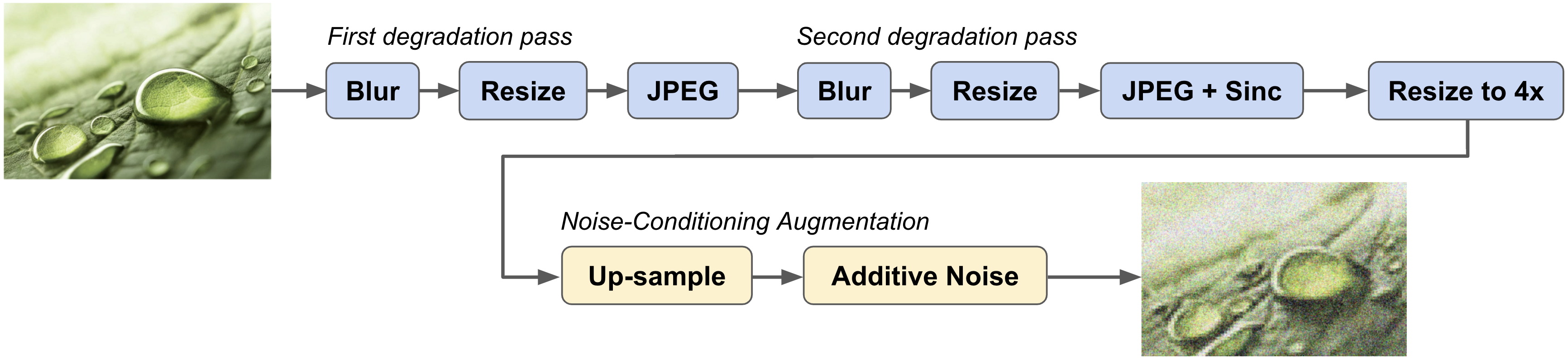
SR3+ is trained with a data-augmentation pipeline that comprises multiple types of degradation, including image blur, additive noise, JPEG compression and down-sampling. While the use of multiple parametric deformations in super-resolution training pipelines are common (Zhang et al., 2021; Wang et al., 2021a), Wang et al. (2021b) found that applying repeated sequences of deformations, called higher-order deformations, has a substantial impact on OOD generalization. For simplicity and comparability to Real-ESRGAN, SR3+ uses the same degradation pipeline, but without additive noise (see Figure 2). Empirically, we found in our preliminary experiments that noise conditioning augmentation (explained later) is better than including noise in the degradation pipeline. Training a 400M parameter model on the same dataset as Real-ESRGAN, but with noise in the degradations instead of noise conditioning augmentation, we obtain an FID(10k) score of 42.58 (vs. 36.28, see Table 1). For completeness, we now document all the degradation hyperparameters. These should match those used by Wang et al. (2021b).
Blur. Four blur filters are used, i.e., Gaussian, generalized Gaussian, a plateau-based kernel, and a sinc (selected with probabilities 0.63, 0.135, 0.135 and 0.1). With probability the Gaussians are isotropic, and anisotrpic otherwise. The plateau kernel is isotropic with probability . When anisotropic, kernels are rotated by a random angle in . For isotropic kernels, . For anisotropic kernels, . The kernel radius is random between 3 and 11 pixels (with only with odd value). For the sinc-filter blur, is randomly selected from when and from otherwise. For generalized Gaussians, the shape parameter is sampled from ; it is sampled from for the plateau filter. The second blur is omitted with probability 0.2; but when used, .
Resizing. Images are resized in one of three (equiprobable) ways, i.e., area resizing, bicubic interpolation, or bilinear interpolation. The scale factor is random in for the first stage resize, and in for the second.
JPEG compression. The JPEG quality factor is drawn randomly from . In the second stage we also apply a sinc filter (described above), either before or after the JPEG compression (with equal probability).
After two stages of degradations, as illustrated in Fig. 2, the image is resized using bicubic interpolation to the desired magnification between the original HR image and the LR degraded image. SR3+ is trained for magnification.
4.3 Noise Conditioning Augmentation
Noise conditioning was first used in cascaded diffusion models (Ho et al., 2022; Saharia et al., 2022b). It was introduced so that super-resolution models in a cascade can be self-supervised with down-sampling, while at test time it will receive input from the previous model in the cascade. Noise conditioning augmentation provided robustness to the distribution of inputs from the previous stage, even though the stages are trained independently. While the degradation pipeline should already improve robustness, it is natural to ask whether further robustness can be achieved by also including this technique.
In essence, noise-conditioning augmentation entails addding noise to the up-sampled LR input, but also providing the noise level to the neural denoiser. At training time, for each LR image in a minibatch, it entails
-
1.
Sample .
-
2.
Add noise to get , reusing the marginal distribution of the diffusion forward process.
-
3.
Condition the model on instead of , and we also condition the model on (a positional embedding of) .
The model learns to handle input signals at different noise levels . In practice, we set ; beyond this value, the input signal to noise ratio is too low for effective training.
At test time, the noise level hyper-parameter in noise-conditioning augmentation, , provides a trade-off between alignment with the LR input and hallucination by the generative model. As increases, more high-frequency detail is lost, so the model is forced to rely more on its knowledge of natural images than on the conditioning signal per se. We find that this enables the hallucination of realistic textures and visual detail.
| Bicubic | Real-ESRGAN | SR3+ (40M) | SR3+ (400M) | SR3+ (400M,61M) | Ground Truth |
|---|---|---|---|---|---|
 |
 |
 |
 |
 |
 |
 |
 |
 |
 |
 |
 |
 |
 |
 |
 |
 |
 |
 |
 |
 |
 |
 |
 |
 |
 |
 |
 |
 |
 |
 |
 |
 |
 |
 |
 |
5 Experiments
SR3+ is trained with a combination of degradations and noise-conditioning augmentation on multiple datasets, and applied zero-shot to test data. We use ablations to determine the impact of the different forms of augmentation, of model size, and dataset size. Here, we focus on the blind super-resolution task with a magnification factor. For baselines, we use SR3 (Saharia et al., 2022c) and the previous state-of-the-art in blind super-resolution, i.e., Real-ESRGAN (Wang et al., 2021b).
Like SR3, the LR input up-sampled by using bicubic interpolation. The output samples for SR3 and SR3+ are obtained using DDPM ancestral sampling (Ho et al., 2020) with 256 denoising steps. For simplicity and to train with continuous timesteps, we use the cosine log-SNR schedule introduced by Ho & Salimans (2022).
Training. For fair comparison with Real-ESRGAN, we first train SR3+ on the datasets used to train Real-ESRGAN (Wang et al., 2021b); namely, DF2K+OST (Agustsson & Timofte, 2017), a combination of Div2K (800 images), Flick2K (2650 images) and OST300 (300 images). To explore the impact of scaling, we also train on a large dataset of 61M images, combining a collection of in-house images with DF2K+OST.
| SR Model (Parameter Count, Dataset) | FID(10k) | PSNR | SSIM | |||
| RealSR | DRealSR | RealSR | DRealSR | RealSR | DRealSR | |
| Real-ESRGAN | 34.21 | 37.22 | 25.14 | 25.85 | 0.7279 | 0.7808 |
| SR3+ (40M, DF2K + OST) | 31.97 | 40.26 | 24.84 | 25.18 | 0.6827 | 0.7201 |
| SR3+ (400M, DF2K + OST) | 27.34 | 36.28 | 23.84 | 24.36 | 0.662 | 0.719 |
| SR3+ (400M, 61M Dataset) | 24.32 | 32.37 | 24.89 | 25.74 | 0.6922 | 0.7547 |
During training, following Real-ESRGAN, we extract a random crop for each image and then apply the degradation pipeline (Fig. 2). The degraded image is then resized to (for magnification). LR images is then up-sampled using bicubic interpolation to from which center crops yield images for training the task. Since the model is convolutional, we can then apply it to arbitrary resolutions and aspect ratios at test time.
For the results below, SR3+ and all ablations are trained on the same data with the same hyper-parameters. Note that SR3+ reduces to SR3 when the degradations and noise-conditioning augmentation are removed. All models were trained for 1.5M steps, using a batch size of 256 for models trained on DF2K+OST and 512 otherwise. We additionally consider two models sizes, with 40M and 400M weights. The smaller enables direct comparison to Real-ESRGAN, which also has about 40M parameters. The larger model exposes the impact of model scaling.
Testing. For testing, as mentioned above, we focus on zero-shot application to test datasets disjoint from those used for training. In all experiments and ablations, we use the RealSR (Cai et al., 2019) v3 and DRealSR (Wei et al., 2020) datasets for evaluation. RealSR has 400 paired low-and-high-resolution images, from which we compute 25 random but aligned and crops per image pair. This yields a fixed test set of 10,000 image pairs. DRealSR contains more than 10,000 image pairs, so we instead extract and center crops for 10,000 random images.
Model performance is assessed with a combination of PSNR, SSIM (Wang et al., 2004) and FID (10k) (Heusel et al., 2017). While reference-based metrics like PSNR and SSIM are useful for small magnification factors, at magnifications of 4x and larger, especially when using a generative model and noise-conditioning augmentation in testing, the posterior distribution is complex, and one expects significant diversity in the output in contrast to regression models.
For SR tasks with multi-modal posterios, e.g., at larger magnifications, reference-based metrics do not agree well with human preferences. While blurry images tend to minimize RMSE from ground truth, they are scored worse by human observers (Chen et al., 2018; Dahl et al., 2017; Menon et al., 2020; Saharia et al., 2022c). In particular PSNR and SSIM tend to over-penalize plausible but infered high-frequency detail that may not agree precisely with ground truth images. We nevertheless consider reconstruction metrics to remain important to evaluate SR models, as they reward alignment and this is a desirable property (especially on regions with less high-frequency details).
In addition to PSNR and SSIM, we also report FID, which on sufficiently larger datasets provides a measure of aggregate statistical similarly with ground truth image data. This correlates better with human quality assessment. As generative models are applied to more difficult inputs, or with large amounts of NCA or larger magnifications, we will need to rely more on FID and similar measures. For in such cases, we will be relying on model inference to capture stats of natural images, and this requires a much larger model, as generative models are hard to learn. So one would expect larger data and larger models would perform better.
| Input | SR3+ | No noise cond. aug. | No degradations | SR3 (ablate both) |
|---|---|---|---|---|
 |
 |
 |
 |
 |
 |
 |
 |
 |
 |
 |
 |
 |
 |
 |
5.1 Comparison with Real-ESRGAN and SR3
| SR Model (400M parameters, 61M Dataset) | FID(10k) | PSNR | SSIM | |||
| RealSR | DRealSR | RealSR | DRealSR | RealSR | DRealSR | |
| SR3+ | 24.32 | 32.37 | 24.89 | 25.74 | 0.6922 | 0.7547 |
| SR3+ (no noise cond. aug.) | 34.20 | 49.93 | 22.34 | 22.28 | 0.6469 | 0.6994 |
| SR3+ (no degradations) | 36.93 | 44.18 | 25.00 | 26.22 | 0.6824 | 0.7687 |
| SR3 (i.e., ablating both) | 85.77 | 93.05 | 27.89 | 28.25 | 0.784 | 0.83 |
As previously discussed, we compare SR3+ models of different sizes with Real-ESRGAN, the previous state-of-the-art model on blind super-resolution, all trained on the same data. Moreover, in order to attain the best possible results in general, we compare our best SR3+ model trained on said data with an identical one that was instead trained on the much larger 61M-image dataset (and with twice the batch size). For evaluation, we perform a grid sweep over from 0 to 0.4, with increments of 0.05, and report results with , which we consistently find to be the best value. We provide side-by-side comparisons in Figure 3, and show quantitative results in Table 1.
We find that, with a 40M-parameter network, SR3+ achieves competitive FID scores with Real-ESRGAN, achieving better scores on RealSR but slightly worse on DRealSR. Qualitatively, it creates more realistic textures without significant oversmoothing or saturation, but it does worse for certain kinds of images where we care about accurate high-frequency detail, such as images with text. The results and realism of the images improve significantly with a 400M-parameter SR3+ model, outperforming Real-ESRGAN on FID scores when trained on the same dataset, and this gap is furthered widened simply by training on the much larger dataset. In the latter case, some of the failure modes of the earlier models (e.g., the text case) are also alleviated, and rougher textures are more coherent within the images. We provide additional samples in the Supplementary Material.
SR3+ does not outperform on reference-based metrics (PSNR, SSIM) are slightly worse, but this expected from strong generative models with either larger magnification factors or larger noise-conditioning augmentation (where the generative model is forced to infer more details). This is also shown by prior work (Chen et al., 2018; Dahl et al., 2017; Menon et al., 2020; Saharia et al., 2022c). We verify this empirically in the samples shown in Figure 4 and Table 2, where, notably, SR3 attains better PSNR and SSIM scores, but the model produces blurry results in the blind task. In the 4x magnification task starting from 64x64, can be very multimodal (especially on high-frequency details), and these metrics overpenalize plausible but hallucinated high-frequency details.
5.2 Ablation studies
We now empirically demonstrate the importance of our main contributions, which we recall are (1) the higher-order degradation scheme and (2) noise conditioning augmentation. We conduct an ablation study using our strongest model, i.e., the 400M-parameter SR3+ model trained on the 61M-image dataset, as worse models break more dramatically upon removing said components. We train similar models as our strongest SR3+ model: one without noise conditioning augmentation, one without the higher-order degradations, and one with neither (which is equivalent to an SR3 model, though using the UNetv3 architecture (Saharia et al., 2022b) and in a larger dataset than in the original work). We then compare FID, PSNR and SSIM on the blind SR task, as before. Whenever using noise-conditioning augmentation, we set . Results are included in Table 2 and a sample comparison in Figure 4.
Our results show that FID scores increase significantly upon the removal of either of our main contributions (by over 10 points in all cases). And, upon removing both, FID scores are much worse, as this metric punishes the consistent blurriness of SR3 when applied in the wild to out-of-distribution images. We also observe that, specifically without the higher-order degradations, we also observe some bluriness and a slight improvement across reconstruction metrics. With the SR3 model, which qualitatively appears to suffer most from blur in generations, both PSNR and SSIM improve significantly, and, interestingly enough, sufficiently to outperform Real-ESRGAN in both metrics and both evaluation datasets.
5.3 Noise conditioning augmentation at test time
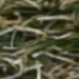
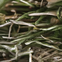
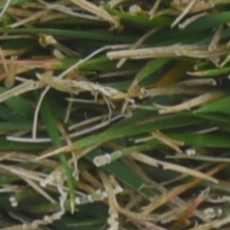
Recall that, due to the use of noise conditioning augmentation, we introduce a degree of freedom at sampling time that we are free to play with. Intuitively, it would seem that using would be most appropriate, as adding noise removes some information from the conditioning low-resolution input. Empirically, however, we find that using a nonzero can often lead to better results; especially on images where highly detailed textures are desirable. To demonstrate this, we present a comparison of FID scores across different values of in Figure 6, for our two 400M-parameter SR3+ models (recall, one trained on DF2K+OST and one on the 61M-image dataset). We additionally include samples from the SR3+ model trained on the 61M-image dataset in Figure 5.
| Input | Ground truth | |||||
|---|---|---|---|---|---|---|
 |
 |
 |
 |
 |
 |
 |
 |
 |
 |
 |
 |
 |
 |
 |
 |
 |
 |
 |
 |
 |
For both models and both evaluation datasets, we find that FID scores can visibly drop when using noise conditioning augmentation at test time, with the best value often about . With the model trained on the 61M-image dataset, we curiously find that more aggressive noise conditioning augmentation can be used at test time while still attaining better FID scores than with . In our samples, we show that the effect of using small amounts of test-time noise conditioning augmentation has a subtle but beneficial effect: higher-quality textures appear and there is less bluriness than without any noise, and alignment to the conditioning image remains good or can even improve (e.g., the flower pot seemed to shift up without noise). As we increase , however, we begin to see initially small but increasingly more apparent misalignment to the conditioning image, as more high-frequency information is destroyed with increasing amounts of noise applied to the conditioning signal. This forces the model to rely on its own knowledge to hallucinate such details and textures, which can be beneficial in most cases (but less so with, e.g., text).
6 Conclusion
In this work, we propose SR3+, a diffusion model for blind super-resolution. By combining two recent techniques for image enhancement, a higher order degradation scheme and noise conditioning augmentation, SR3+ achieves state-of-the-art FID scores across test datasets for blind super-resolution. We further improve quantitative and qualitative results significantly just by training on a much larger dataset. Unlike prior work, SR3+ is both robust to out-of-distribution inputs, and can generate realistic textures in a controllable manner, as test-time noise conditioning augmentation can force the model to rely on more of its own knowledge to infer high-frequency details. SR3+ excels at natural images, and with enough data, it performs reasonably well on other images such as those with text. We are most excited about SR3+ improving diffusion model quality and robustness more broadly, especially those relying on cascading (Ho et al., 2022), e.g., text-to-image models.
SR3+ nevertheless has some limitations. When using noise conditioning augmentation, some failure modes can be observed such as gibberish text, and more training steps might needed for convergence as the task becomes more challenging than with conditioning signals that are always clean. We believe that models with larger capacity (i.e., parameter count), as well as improvements on neural architectures, could address these issues in future work.
References
- Agustsson & Timofte (2017) Agustsson, E. and Timofte, R. Ntire 2017 challenge on single image super-resolution: Dataset and study. In 2017 IEEE Conference on Computer Vision and Pattern Recognition Workshops (CVPRW), pp. 1122–1131, 2017. doi: 10.1109/CVPRW.2017.150.
- Ahn et al. (2018) Ahn, N., Kang, B., and Sohn, K.-A. Fast, accurate, and lightweight super-resolution with cascading residual network. In Proceedings of the European conference on computer vision (ECCV), pp. 252–268, 2018.
- Cai et al. (2019) Cai, J., Zeng, H., Yong, H., Cao, Z., and Zhang, L. Toward real-world single image super-resolution: A new benchmark and a new model. In Proceedings of the IEEE/CVF International Conference on Computer Vision, pp. 3086–3095, 2019.
- Chen et al. (2018) Chen, Y., Tai, Y., Liu, X., Shen, C., and Yang, J. Fsrnet: End-to-end learning face super-resolution with facial priors. In Proceedings of the IEEE conference on computer vision and pattern recognition, pp. 2492–2501, 2018.
- Choi & Kim (2017) Choi, J.-S. and Kim, M. A deep convolutional neural network with selection units for super-resolution. In 2017 IEEE Conference on Computer Vision and Pattern Recognition Workshops (CVPRW), pp. 1150–1156, 2017. doi: 10.1109/CVPRW.2017.153.
- Dahl et al. (2017) Dahl, R., Norouzi, M., and Shlens, J. Pixel recursive super resolution. In Proceedings of the IEEE international conference on computer vision, pp. 5439–5448, 2017.
- Dhariwal & Nichol (2021) Dhariwal, P. and Nichol, A. Diffusion models beat gans on image synthesis. Advances in Neural Information Processing Systems, 34:8780–8794, 2021.
- Dong et al. (2015) Dong, C., Loy, C. C., He, K., and Tang, X. Image super-resolution using deep convolutional networks. IEEE transactions on pattern analysis and machine intelligence, 38(2):295–307, 2015.
- Dong et al. (2016) Dong, C., Loy, C. C., and Tang, X. Accelerating the super-resolution convolutional neural network. In European conference on computer vision, pp. 391–407. Springer, 2016.
- Fan et al. (2017) Fan, Y., Shi, H., Yu, J., Liu, D., Han, W., Yu, H., Wang, Z., Wang, X., and Huang, T. S. Balanced two-stage residual networks for image super-resolution. In 2017 IEEE Conference on Computer Vision and Pattern Recognition Workshops (CVPRW), pp. 1157–1164, 2017. doi: 10.1109/CVPRW.2017.154.
- Heusel et al. (2017) Heusel, M., Ramsauer, H., Unterthiner, T., Nessler, B., and Hochreiter, S. Gans trained by a two time-scale update rule converge to a local nash equilibrium. Advances in neural information processing systems, 30, 2017.
- Ho & Salimans (2022) Ho, J. and Salimans, T. Classifier-free diffusion guidance. arXiv preprint arXiv:2207.12598, 2022.
- Ho et al. (2020) Ho, J., Jain, A., and Abbeel, P. Denoising diffusion probabilistic models. Advances in Neural Information Processing Systems, 33:6840–6851, 2020.
- Ho et al. (2022) Ho, J., Saharia, C., Chan, W., Fleet, D. J., Norouzi, M., and Salimans, T. Cascaded diffusion models for high fidelity image generation. J. Mach. Learn. Res., 23:47–1, 2022.
- Kim et al. (2016a) Kim, J., Lee, J. K., and Lee, K. M. Accurate image super-resolution using very deep convolutional networks. In Proceedings of the IEEE conference on computer vision and pattern recognition, pp. 1646–1654, 2016a.
- Kim et al. (2016b) Kim, J., Lee, J. K., and Lee, K. M. Deeply-recursive convolutional network for image super-resolution. In Proceedings of the IEEE conference on computer vision and pattern recognition, pp. 1637–1645, 2016b.
- Kingma & Welling (2013) Kingma, D. P. and Welling, M. Auto-encoding variational bayes. arXiv preprint arXiv:1312.6114, 2013.
- Lai et al. (2017) Lai, W.-S., Huang, J.-B., Ahuja, N., and Yang, M.-H. Deep laplacian pyramid networks for fast and accurate super-resolution. In Proceedings of the IEEE conference on computer vision and pattern recognition, pp. 624–632, 2017.
- Li et al. (2022) Li, H., Yang, Y., Chang, M., Chen, S., Feng, H., Xu, Z., Li, Q., and Chen, Y. Srdiff: Single image super-resolution with diffusion probabilistic models. Neurocomputing, 479:47–59, 2022.
- Liang et al. (2021) Liang, J., Zhang, K., Gu, S., Van Gool, L., and Timofte, R. Flow-based kernel prior with application to blind super-resolution. In Proceedings of the IEEE/CVF Conference on Computer Vision and Pattern Recognition, pp. 10601–10610, 2021.
- Lim et al. (2017) Lim, B., Son, S., Kim, H., Nah, S., and Mu Lee, K. Enhanced deep residual networks for single image super-resolution. In Proceedings of the IEEE conference on computer vision and pattern recognition workshops, pp. 136–144, 2017.
- Liu et al. (2021) Liu, A., Liu, Y., Gu, J., Qiao, Y., and Dong, C. Blind image super-resolution: A survey and beyond. arXiv preprint arXiv:2107.03055, 2021.
- Luo et al. (2021) Luo, Z., Huang, Y., Li, S., Wang, L., and Tan, T. End-to-end alternating optimization for blind super resolution. arXiv preprint arXiv:2105.06878, 2021.
- Menon et al. (2020) Menon, S., Damian, A., Hu, S., Ravi, N., and Rudin, C. Pulse: Self-supervised photo upsampling via latent space exploration of generative models. In Proceedings of the ieee/cvf conference on computer vision and pattern recognition, pp. 2437–2445, 2020.
- Patel et al. (2021) Patel, M., Purohit, M., Shah, J., and Patil, H. A. Cinc-gan for effective f 0 prediction for whisper-to-normal speech conversion. In 2020 28th European Signal Processing Conference (EUSIPCO), pp. 411–415. IEEE, 2021.
- Rombach et al. (2022) Rombach, R., Blattmann, A., Lorenz, D., Esser, P., and Ommer, B. High-resolution image synthesis with latent diffusion models. In Proceedings of the IEEE/CVF Conference on Computer Vision and Pattern Recognition, pp. 10684–10695, 2022.
- Saharia et al. (2022a) Saharia, C., Chan, W., Chang, H., Lee, C., Ho, J., Salimans, T., Fleet, D., and Norouzi, M. Palette: Image-to-image diffusion models. In ACM SIGGRAPH 2022 Conference Proceedings, pp. 1–10, 2022a.
- Saharia et al. (2022b) Saharia, C., Chan, W., Saxena, S., Li, L., Whang, J., Denton, E., Ghasemipour, S. K. S., Ayan, B. K., Mahdavi, S. S., Lopes, R. G., et al. Photorealistic text-to-image diffusion models with deep language understanding. arXiv preprint arXiv:2205.11487, 2022b.
- Saharia et al. (2022c) Saharia, C., Ho, J., Chan, W., Salimans, T., Fleet, D. J., and Norouzi, M. Image super-resolution via iterative refinement. IEEE Transactions on Pattern Analysis and Machine Intelligence, 2022c.
- Shi et al. (2016) Shi, W., Caballero, J., Huszár, F., Totz, J., Aitken, A. P., Bishop, R., Rueckert, D., and Wang, Z. Real-time single image and video super-resolution using an efficient sub-pixel convolutional neural network. In Proceedings of the IEEE conference on computer vision and pattern recognition, pp. 1874–1883, 2016.
- Shocher et al. (2018) Shocher, A., Cohen, N., and Irani, M. “zero-shot” super-resolution using deep internal learning. In Proceedings of the IEEE conference on computer vision and pattern recognition, pp. 3118–3126, 2018.
- Sohl-Dickstein et al. (2015) Sohl-Dickstein, J., Weiss, E., Maheswaranathan, N., and Ganguli, S. Deep unsupervised learning using nonequilibrium thermodynamics. In International Conference on Machine Learning, pp. 2256–2265. PMLR, 2015.
- Song & Ermon (2019) Song, Y. and Ermon, S. Generative modeling by estimating gradients of the data distribution. Advances in Neural Information Processing Systems, 32, 2019.
- Song et al. (2020) Song, Y., Sohl-Dickstein, J., Kingma, D. P., Kumar, A., Ermon, S., and Poole, B. Score-based generative modeling through stochastic differential equations. arXiv preprint arXiv:2011.13456, 2020.
- Tai et al. (2017) Tai, Y., Yang, J., and Liu, X. Image super-resolution via deep recursive residual network. In 2017 IEEE Conference on Computer Vision and Pattern Recognition (CVPR), pp. 2790–2798, 2017. doi: 10.1109/CVPR.2017.298.
- Thanh-Tung & Tran (2020) Thanh-Tung, H. and Tran, T. Catastrophic forgetting and mode collapse in gans. In 2020 international joint conference on neural networks (ijcnn), pp. 1–10. IEEE, 2020.
- Wang et al. (2021a) Wang, L., Wang, Y., Dong, X., Xu, Q., Yang, J., An, W., and Guo, Y. Unsupervised degradation representation learning for blind super-resolution. In Proceedings of the IEEE/CVF Conference on Computer Vision and Pattern Recognition, pp. 10581–10590, 2021a.
- Wang et al. (2021b) Wang, X., Xie, L., Dong, C., and Shan, Y. Real-esrgan: Training real-world blind super-resolution with pure synthetic data. In Proceedings of the IEEE/CVF International Conference on Computer Vision, pp. 1905–1914, 2021b.
- Wang et al. (2004) Wang, Z., Bovik, A. C., Sheikh, H. R., and Simoncelli, E. P. Image quality assessment: from error visibility to structural similarity. IEEE transactions on image processing, 13(4):600–612, 2004.
- Wei et al. (2020) Wei, P., Xie, Z., Lu, H., Zhan, Z., Ye, Q., Zuo, W., and Lin, L. Component divide-and-conquer for real-world image super-resolution. In European Conference on Computer Vision, pp. 101–117. Springer, 2020.
- Whang et al. (2022) Whang, J., Delbracio, M., Talebi, H., Saharia, C., Dimakis, A. G., and Milanfar, P. Deblurring via stochastic refinement. In Proceedings of the IEEE/CVF Conference on Computer Vision and Pattern Recognition, pp. 16293–16303, 2022.
- Yan et al. (2021) Yan, Y., Liu, C., Chen, C., Sun, X., Jin, L., Peng, X., and Zhou, X. Fine-grained attention and feature-sharing generative adversarial networks for single image super-resolution. IEEE Transactions on Multimedia, 24:1473–1487, 2021.
- Yin et al. (2021) Yin, G., Wang, W., Yuan, Z., Yu, D., Sun, S., and Wang, C. Conditional meta-network for blind super-resolution with multiple degradations. arXiv preprint arXiv:2104.03926, 2021.
- Yoo et al. (2022) Yoo, J.-S., Kim, D.-W., Lu, Y., and Jung, S.-W. Rzsr: Reference-based zero-shot super-resolution with depth guided self-exemplars. IEEE Transactions on Multimedia, 2022.
- Zhang et al. (2021) Zhang, K., Liang, J., Van Gool, L., and Timofte, R. Designing a practical degradation model for deep blind image super-resolution. In Proceedings of the IEEE/CVF International Conference on Computer Vision, pp. 4791–4800, 2021.
- Zhang et al. (2018) Zhang, Y., Li, K., Li, K., Wang, L., Zhong, B., and Fu, Y. Image super-resolution using very deep residual channel attention networks. In Proceedings of the European conference on computer vision (ECCV), pp. 286–301, 2018.
Appendix A Additional sample comparisons between SR3+ and other models
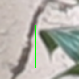
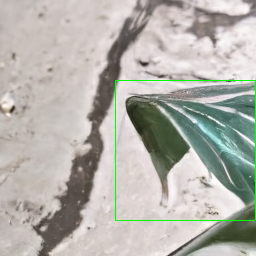
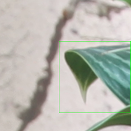
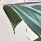
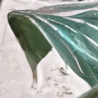
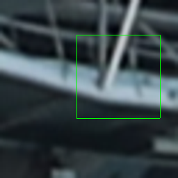
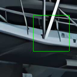
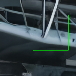
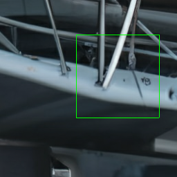
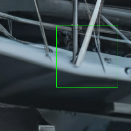
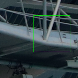
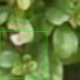
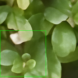
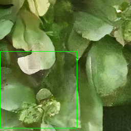
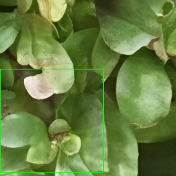
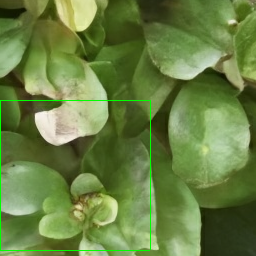
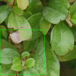
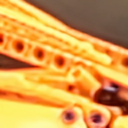
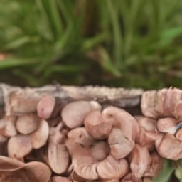
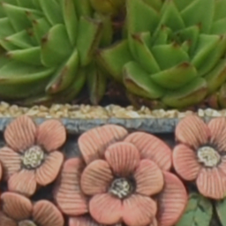
We provide more side-by-side comparisons of our best SR3+ model with SR3 and Real-ESRGAN. We display a single zoomed-in crop for each image to emphasize that SR3+ outperforms prior work.
| Input | SR3 | Real-ESRGAN | SR3+ (Ours) | Ground Truth |
|---|---|---|---|---|
![[Uncaptioned image]](/html/2302.07864/assets/images/fig2/7366/input_boxed.png) |
![[Uncaptioned image]](/html/2302.07864/assets/images/fig2/7366/sr3_boxed.png) |
![[Uncaptioned image]](/html/2302.07864/assets/images/fig2/7366/realesrgan_boxed.png) |
![[Uncaptioned image]](/html/2302.07864/assets/images/fig2/7366/res_400m_getty_boxed.png) |
![[Uncaptioned image]](/html/2302.07864/assets/images/fig2/7366/output_boxed.png) |
![[Uncaptioned image]](/html/2302.07864/assets/images/fig2/7366/input_crop.png) |
![[Uncaptioned image]](/html/2302.07864/assets/images/fig2/7366/sr3_crop.png) |
![[Uncaptioned image]](/html/2302.07864/assets/images/fig2/7366/realesrgan_crop.png) |
![[Uncaptioned image]](/html/2302.07864/assets/images/fig2/7366/res_400m_getty_crop.png) |
![[Uncaptioned image]](/html/2302.07864/assets/images/fig2/7366/output_crop.png) |
![[Uncaptioned image]](/html/2302.07864/assets/images/fig2/4141/input_boxed.png) |
![[Uncaptioned image]](/html/2302.07864/assets/images/fig2/4141/sr3_boxed.png) |
![[Uncaptioned image]](/html/2302.07864/assets/images/fig2/4141/realesrgan_boxed.png) |
![[Uncaptioned image]](/html/2302.07864/assets/images/fig2/4141/res_400m_getty_boxed.png) |
![[Uncaptioned image]](/html/2302.07864/assets/images/fig2/4141/output_boxed.png) |
![[Uncaptioned image]](/html/2302.07864/assets/images/fig2/4141/input_crop.png) |
![[Uncaptioned image]](/html/2302.07864/assets/images/fig2/4141/sr3_crop.png) |
![[Uncaptioned image]](/html/2302.07864/assets/images/fig2/4141/realesrgan_crop.png) |
![[Uncaptioned image]](/html/2302.07864/assets/images/fig2/4141/res_400m_getty_crop.png) |
![[Uncaptioned image]](/html/2302.07864/assets/images/fig2/4141/output_crop.png) |
![[Uncaptioned image]](/html/2302.07864/assets/images/appendix/16/input_boxed.png) |
![[Uncaptioned image]](/html/2302.07864/assets/images/appendix/16/sr3_boxed.png) |
![[Uncaptioned image]](/html/2302.07864/assets/images/appendix/16/realesrgan_boxed.png) |
![[Uncaptioned image]](/html/2302.07864/assets/images/appendix/16/res_400m_getty_boxed.png) |
![[Uncaptioned image]](/html/2302.07864/assets/images/appendix/16/output_boxed.png) |
![[Uncaptioned image]](/html/2302.07864/assets/images/appendix/16/input_crop.png) |
![[Uncaptioned image]](/html/2302.07864/assets/images/appendix/16/sr3_crop.png) |
![[Uncaptioned image]](/html/2302.07864/assets/images/appendix/16/realesrgan_crop.png) |
![[Uncaptioned image]](/html/2302.07864/assets/images/appendix/16/res_400m_getty_crop.png) |
![[Uncaptioned image]](/html/2302.07864/assets/images/appendix/16/output_crop.png) |
| Input | SR3 | Real-ESRGAN | SR3+ (Ours) | Ground Truth |
|---|---|---|---|---|
![[Uncaptioned image]](/html/2302.07864/assets/images/appendix/2022/input_boxed.png) |
![[Uncaptioned image]](/html/2302.07864/assets/images/appendix/2022/sr3_boxed.png) |
![[Uncaptioned image]](/html/2302.07864/assets/images/appendix/2022/realesrgan_boxed.png) |
![[Uncaptioned image]](/html/2302.07864/assets/images/appendix/2022/ours_boxed.png) |
![[Uncaptioned image]](/html/2302.07864/assets/images/appendix/2022/output_boxed.png) |
![[Uncaptioned image]](/html/2302.07864/assets/images/appendix/2022/input_crop.png) |
![[Uncaptioned image]](/html/2302.07864/assets/images/appendix/2022/sr3_crop.png) |
![[Uncaptioned image]](/html/2302.07864/assets/images/appendix/2022/realesrgan_crop.png) |
![[Uncaptioned image]](/html/2302.07864/assets/images/appendix/2022/ours_crop.png) |
![[Uncaptioned image]](/html/2302.07864/assets/images/appendix/2022/output_crop.png) |
![[Uncaptioned image]](/html/2302.07864/assets/images/appendix/3305/input_boxed.png) |
![[Uncaptioned image]](/html/2302.07864/assets/images/appendix/3305/sr3_boxed.png) |
![[Uncaptioned image]](/html/2302.07864/assets/images/appendix/3305/realesrgan_boxed.png) |
![[Uncaptioned image]](/html/2302.07864/assets/images/appendix/3305/ours_boxed.png) |
![[Uncaptioned image]](/html/2302.07864/assets/images/appendix/3305/output_boxed.png) |
![[Uncaptioned image]](/html/2302.07864/assets/images/appendix/3305/input_crop.png) |
![[Uncaptioned image]](/html/2302.07864/assets/images/appendix/3305/sr3_crop.png) |
![[Uncaptioned image]](/html/2302.07864/assets/images/appendix/3305/realesrgan_crop.png) |
![[Uncaptioned image]](/html/2302.07864/assets/images/appendix/3305/ours_crop.png) |
![[Uncaptioned image]](/html/2302.07864/assets/images/appendix/3305/output_crop.png) |
![[Uncaptioned image]](/html/2302.07864/assets/images/appendix/3400/input_boxed.png) |
![[Uncaptioned image]](/html/2302.07864/assets/images/appendix/3400/sr3_boxed.png) |
![[Uncaptioned image]](/html/2302.07864/assets/images/appendix/3400/realesrgan_boxed.png) |
![[Uncaptioned image]](/html/2302.07864/assets/images/appendix/3400/ours_boxed.png) |
![[Uncaptioned image]](/html/2302.07864/assets/images/appendix/3400/output_boxed.png) |
![[Uncaptioned image]](/html/2302.07864/assets/images/appendix/3400/input_crop.png) |
![[Uncaptioned image]](/html/2302.07864/assets/images/appendix/3400/sr3_crop.png) |
![[Uncaptioned image]](/html/2302.07864/assets/images/appendix/3400/realesrgan_crop.png) |
![[Uncaptioned image]](/html/2302.07864/assets/images/appendix/3400/ours_crop.png) |
![[Uncaptioned image]](/html/2302.07864/assets/images/appendix/3400/output_crop.png) |
| Input | SR3 | Real-ESRGAN | SR3+ (Ours) | Ground Truth |
|---|---|---|---|---|
![[Uncaptioned image]](/html/2302.07864/assets/images/appendix/3702/input_boxed.png) |
![[Uncaptioned image]](/html/2302.07864/assets/images/appendix/3702/sr3_boxed.png) |
![[Uncaptioned image]](/html/2302.07864/assets/images/appendix/3702/realesrgan_boxed.png) |
![[Uncaptioned image]](/html/2302.07864/assets/images/appendix/3702/ours_boxed.png) |
![[Uncaptioned image]](/html/2302.07864/assets/images/appendix/3702/output_boxed.png) |
![[Uncaptioned image]](/html/2302.07864/assets/images/appendix/3702/input_crop.png) |
![[Uncaptioned image]](/html/2302.07864/assets/images/appendix/3702/sr3_crop.png) |
![[Uncaptioned image]](/html/2302.07864/assets/images/appendix/3702/realesrgan_crop.png) |
![[Uncaptioned image]](/html/2302.07864/assets/images/appendix/3702/ours_crop.png) |
![[Uncaptioned image]](/html/2302.07864/assets/images/appendix/3702/output_crop.png) |
![[Uncaptioned image]](/html/2302.07864/assets/images/appendix/5741/input_boxed.png) |
![[Uncaptioned image]](/html/2302.07864/assets/images/appendix/5741/sr3_boxed.png) |
![[Uncaptioned image]](/html/2302.07864/assets/images/appendix/5741/realesrgan_boxed.png) |
![[Uncaptioned image]](/html/2302.07864/assets/images/appendix/5741/ours_boxed.png) |
![[Uncaptioned image]](/html/2302.07864/assets/images/appendix/5741/output_boxed.png) |
![[Uncaptioned image]](/html/2302.07864/assets/images/appendix/5741/input_crop.png) |
![[Uncaptioned image]](/html/2302.07864/assets/images/appendix/5741/sr3_crop.png) |
![[Uncaptioned image]](/html/2302.07864/assets/images/appendix/5741/realesrgan_crop.png) |
![[Uncaptioned image]](/html/2302.07864/assets/images/appendix/5741/ours_crop.png) |
![[Uncaptioned image]](/html/2302.07864/assets/images/appendix/5741/output_crop.png) |
![[Uncaptioned image]](/html/2302.07864/assets/images/appendix/5756/input_boxed.png) |
![[Uncaptioned image]](/html/2302.07864/assets/images/appendix/5756/sr3_boxed.png) |
![[Uncaptioned image]](/html/2302.07864/assets/images/appendix/5756/realesrgan_boxed.png) |
![[Uncaptioned image]](/html/2302.07864/assets/images/appendix/5756/ours_boxed.png) |
![[Uncaptioned image]](/html/2302.07864/assets/images/appendix/5756/output_boxed.png) |
![[Uncaptioned image]](/html/2302.07864/assets/images/appendix/5756/input_crop.png) |
![[Uncaptioned image]](/html/2302.07864/assets/images/appendix/5756/sr3_crop.png) |
![[Uncaptioned image]](/html/2302.07864/assets/images/appendix/5756/realesrgan_crop.png) |
![[Uncaptioned image]](/html/2302.07864/assets/images/appendix/5756/ours_crop.png) |
![[Uncaptioned image]](/html/2302.07864/assets/images/appendix/5756/output_crop.png) |
| Input | SR3 | Real-ESRGAN | SR3+ (Ours) | Ground Truth |
|---|---|---|---|---|
![[Uncaptioned image]](/html/2302.07864/assets/images/appendix/8691/input_boxed.png) |
![[Uncaptioned image]](/html/2302.07864/assets/images/appendix/8691/sr3_boxed.png) |
![[Uncaptioned image]](/html/2302.07864/assets/images/appendix/8691/realesrgan_boxed.png) |
![[Uncaptioned image]](/html/2302.07864/assets/images/appendix/8691/ours_boxed.png) |
![[Uncaptioned image]](/html/2302.07864/assets/images/appendix/8691/output_boxed.png) |
![[Uncaptioned image]](/html/2302.07864/assets/images/appendix/8691/input_crop.png) |
![[Uncaptioned image]](/html/2302.07864/assets/images/appendix/8691/sr3_crop.png) |
![[Uncaptioned image]](/html/2302.07864/assets/images/appendix/8691/realesrgan_crop.png) |
![[Uncaptioned image]](/html/2302.07864/assets/images/appendix/8691/ours_crop.png) |
![[Uncaptioned image]](/html/2302.07864/assets/images/appendix/8691/output_crop.png) |
![[Uncaptioned image]](/html/2302.07864/assets/images/appendix/9146/input_boxed.png) |
![[Uncaptioned image]](/html/2302.07864/assets/images/appendix/9146/sr3_boxed.png) |
![[Uncaptioned image]](/html/2302.07864/assets/images/appendix/9146/realesrgan_boxed.png) |
![[Uncaptioned image]](/html/2302.07864/assets/images/appendix/9146/ours_boxed.png) |
![[Uncaptioned image]](/html/2302.07864/assets/images/appendix/9146/output_boxed.png) |
![[Uncaptioned image]](/html/2302.07864/assets/images/appendix/9146/input_crop.png) |
![[Uncaptioned image]](/html/2302.07864/assets/images/appendix/9146/sr3_crop.png) |
![[Uncaptioned image]](/html/2302.07864/assets/images/appendix/9146/realesrgan_crop.png) |
![[Uncaptioned image]](/html/2302.07864/assets/images/appendix/9146/ours_crop.png) |
![[Uncaptioned image]](/html/2302.07864/assets/images/appendix/9146/output_crop.png) |
![[Uncaptioned image]](/html/2302.07864/assets/images/appendix/9231/input_boxed.png) |
![[Uncaptioned image]](/html/2302.07864/assets/images/appendix/9231/sr3_boxed.png) |
![[Uncaptioned image]](/html/2302.07864/assets/images/appendix/9231/realesrgan_boxed.png) |
![[Uncaptioned image]](/html/2302.07864/assets/images/appendix/9231/ours_boxed.png) |
![[Uncaptioned image]](/html/2302.07864/assets/images/appendix/9231/output_boxed.png) |
![[Uncaptioned image]](/html/2302.07864/assets/images/appendix/9231/input_crop.png) |
![[Uncaptioned image]](/html/2302.07864/assets/images/appendix/9231/sr3_crop.png) |
![[Uncaptioned image]](/html/2302.07864/assets/images/appendix/9231/realesrgan_crop.png) |
![[Uncaptioned image]](/html/2302.07864/assets/images/appendix/9231/ours_crop.png) |
![[Uncaptioned image]](/html/2302.07864/assets/images/appendix/9231/output_crop.png) |
| Input | SR3 | Real-ESRGAN | SR3+ (Ours) | Ground Truth |
|---|---|---|---|---|
![[Uncaptioned image]](/html/2302.07864/assets/images/appendix/455/input_boxed.png) |
![[Uncaptioned image]](/html/2302.07864/assets/images/appendix/455/sr3_boxed.png) |
![[Uncaptioned image]](/html/2302.07864/assets/images/appendix/455/realesrgan_boxed.png) |
![[Uncaptioned image]](/html/2302.07864/assets/images/appendix/455/res_400m_getty_boxed.png) |
![[Uncaptioned image]](/html/2302.07864/assets/images/appendix/455/output_boxed.png) |
![[Uncaptioned image]](/html/2302.07864/assets/images/appendix/455/input_crop.png) |
![[Uncaptioned image]](/html/2302.07864/assets/images/appendix/455/sr3_crop.png) |
![[Uncaptioned image]](/html/2302.07864/assets/images/appendix/455/realesrgan_crop.png) |
![[Uncaptioned image]](/html/2302.07864/assets/images/appendix/455/res_400m_getty_crop.png) |
![[Uncaptioned image]](/html/2302.07864/assets/images/appendix/455/output_crop.png) |
![[Uncaptioned image]](/html/2302.07864/assets/images/appendix/240/input_boxed.png) |
![[Uncaptioned image]](/html/2302.07864/assets/images/appendix/240/sr3_boxed.png) |
![[Uncaptioned image]](/html/2302.07864/assets/images/appendix/240/realesrgan_boxed.png) |
![[Uncaptioned image]](/html/2302.07864/assets/images/appendix/240/res_400m_getty_boxed.png) |
![[Uncaptioned image]](/html/2302.07864/assets/images/appendix/240/output_boxed.png) |
![[Uncaptioned image]](/html/2302.07864/assets/images/appendix/240/input_crop.png) |
![[Uncaptioned image]](/html/2302.07864/assets/images/appendix/240/sr3_crop.png) |
![[Uncaptioned image]](/html/2302.07864/assets/images/appendix/240/realesrgan_crop.png) |
![[Uncaptioned image]](/html/2302.07864/assets/images/appendix/240/res_400m_getty_crop.png) |
![[Uncaptioned image]](/html/2302.07864/assets/images/appendix/240/output_crop.png) |
![[Uncaptioned image]](/html/2302.07864/assets/images/appendix/448/input_boxed.png) |
![[Uncaptioned image]](/html/2302.07864/assets/images/appendix/448/sr3_boxed.png) |
![[Uncaptioned image]](/html/2302.07864/assets/images/appendix/448/realesrgan_boxed.png) |
![[Uncaptioned image]](/html/2302.07864/assets/images/appendix/448/res_400m_getty_boxed.png) |
![[Uncaptioned image]](/html/2302.07864/assets/images/appendix/448/output_boxed.png) |
![[Uncaptioned image]](/html/2302.07864/assets/images/appendix/448/input_crop.png) |
![[Uncaptioned image]](/html/2302.07864/assets/images/appendix/448/sr3_crop.png) |
![[Uncaptioned image]](/html/2302.07864/assets/images/appendix/448/realesrgan_crop.png) |
![[Uncaptioned image]](/html/2302.07864/assets/images/appendix/448/res_400m_getty_crop.png) |
![[Uncaptioned image]](/html/2302.07864/assets/images/appendix/448/output_crop.png) |