Learning Random Access Schemes for Massive Machine-Type Communication with MARL

Abstract

In this paper, we explore various multi-agent reinforcement learning (MARL) techniques to design grant-free random access (RA) schemes for low-complexity, low-power battery operated devices in massive machine-type communication (mMTC) wireless networks. We use value decomposition networks (VDN) and QMIX algorithms with parameter sharing (PS) with centralized training and decentralized execution (CTDE) while maintaining scalability. We then compare the policies learned by VDN, QMIX, and deep recurrent Q-network (DRQN) and explore the impact of including the agent identifiers in the observation vector. We show that the MARL-based RA schemes can achieve a better throughput-fairness trade-off between agents without having to condition on the agent identifiers. We also present a novel correlated traffic model, which is more descriptive of mMTC scenarios, and show that the proposed algorithm can easily adapt to traffic non-stationarities.

Massive machine-type communications, MARL, reinforcement learning, grant-free random access, scalability.

1 INTRODUCTION

The mMTC paradigm is a key component of 5G and will continue to be important in the development of 6G technologies [1]. As the number of Internet of Things (IoT) devices grows, millions of devices with characteristics different from human-type communication will require connectivity [2, 3]. To support mMTC in LTE-A, 3GPP has developed narrowband IoT (NB-IoT) and LTE-Machine-type communication (LTE-M) [4], which fall under the category of low power wide area networks (LPWANs). In addition to these cellular standards, non-cellular LPWAN standards such as Sigfox [5] and LoRa [6] have also been developed. 3GPP’s Rel-17 introduces ’NR-Light’, a new class of devices that is more capable than NB-IoT or LTE-M, but supports different features with a bandwidth larger than NB-IoT/LTE-M but smaller than 5G NR devices. In this paper, we focus on low-power, low-complexity machine-type devices (MTDs) with low data rates (around 1-100 Kbps), where communication is mostly uplink dominated. These devices are also low-cost and battery-operated, with long battery life and sporadic activity. Managing medium access for these devices is challenging, and future wireless communication systems will need to provide massive connectivity to meet these needs.

For devices having such characteristics, grant-free RA schemes are preferred as scheduled access incurs huge signaling overhead [7]. However, RA schemes are prone to collisions and scale poorly. Traditionally, RA schemes such as exponential backoff (EB) [8] employ back-off mechanism at each device to update their transmit probabilities based on the feedback from the receiver. These schemes are relatively simple and decentralized; however, their performance depends on various assumptions such as the traffic arrival process and whether the buffers are saturated. Additionally, the optimal back-off factor for different system parameters is not fixed and may vary [9]. One drawback of EB schemes such as binary exponential backoff (BEB) is the capture effect, where a group of devices occupy the channel for a period of time, causing other devices to be deprived of access and making the technique unfair. Our goal is to design RA schemes for mMTC that not only provide better throughput but are also fair.

Reinforcement learning (RL) algorithms have become a popular method for learning RA policies in wireless networks. These algorithms can adapt to changes in the environment and use past history to learn the transmission probabilities of devices in a decentralized manner. However, many RL solutions are not tailored to the traffic and device characteristics of mMTC systems (details in Section 5), and they also struggle with scalability to large numbers of devices, which is a critical concern in RA schemes for mMTC. This is because mMTC devices often have low computational power and rely on battery power, making it impractical to perform learning at each device. To the best of our knowledge, the scalability issue has not been adequately addressed in previous RL or MARL studies on RA schemes, and it is unclear if the proposed techniques can handle a large number of devices. MARL has several advantages over traditional EB backoff policies, as it allows for the design of multi-objective policies in a decentralized manner, which is not analytically tractable using traditional methods.

Therefore, the objective of this paper is to design grant-free RA schemes for mMTC using MARL to achieve fairness, adaptability to changes in traffic, centralized learning with decentralized execution, and scalability to a large number of devices. Our contributions are listed in the following.

• We present a system model to learn schemes in which the devices can leave and join the network randomly. We do not assume that all the devices in the network have packets as opposed to most of the other works for RA with RL, e.g., [10, 11].

• We use broadcast feedback to reduce the signaling overhead and for energy efficiency. We assume that the feedback is only sent to the active devices and to save energy, the inactive devices do not listen to the feedback signal.

• We present a suitability report of MARL algorithms for our proposed environment. Since we want a single policy for all the devices that can be learned in a CTDE manner; we provide a comparison between some well-known MARL algorithms and how they may or may not be suitable for our environment. We propose VDN and QMIX algorithms to achieve our objectives. We present our simulation results for VDN for a multiple-user multiple physical resource blocks (PRBs) environment and also compare VDN, QMIX and DRQN policies.

• Most of the MARL algorithms that employ CTDE, include an agent-specific identifier into the observation vector of the agents. In case of mMTC, the devices should be able to leave/join the network and the policies should be scalable to a large number of devices. For these reasons, incorporating agent/device identification (ID) is not feasible. We will also show that how the algorithm distributes resources among MTDs fairly when agent IDs are not incorporated and how the algorithms learn an unfair policy when we use agent IDs.

• We present our results for regular or periodic traffic arrival, in which each MTD receives packets following a random process independently. In addition, we present a correlated traffic arrival model in Section 4, that is more suitable for mMTC system. In the correlated traffic arrival model, the devices follow both regular traffic arrivals and also event-driven (ED) traffic arrival. In ED, that is independent of the regular traffic arrival, a subset of MTDs become active together whenever an event happens. We show that our proposed algorithm adapts to different traffic conditions.

2 RELATED WORK

The application of RL to channel access problems in wireless communications goes back to 2010 that used tabular Q-learning [12]. However, it has become popular in the recent years due to the advancements in deep reinforcement learning (DRL). In [13], the authors considered the problem of multiple access where the agents are the base stations to predict the future state of the system. They use recurrent neural network (RNN) and REINFORCE algorithm to learn policies for each agent. In [14], the ALOHA-Q protocol is proposed for a single channel slotted ALOHA scheme that uses an expert-based approach in RL. The goal in that work is for nodes to learn in which time slots the likelihood of packet collisions is reduced. However, the ALOHA-Q depends on the frame structure and each user keeps and updates a separate policy for each time slot in the frame. In [15], the ALOHA-Q is enhanced by removing the frame structure. However, every user still has to keep the number of policies equal to the time slots window it is going to transmit in. Other works such as [10, 16, 11, 17] consider RL-based multiple access works for multiple channels. In [10, 18, 11] deep Q-network (DQN) algorithm is used for multiple user and multiple channel wireless networks. In [16], another DRL algorithm known as actor-critic DRL is used for dynamic channel access. All of these works train agents with the assumption that every device has always a packet in its buffer (saturation state). Moreover, it is not clear whether their algorithms can be scaled for higher number of agents. Interestingly, these works also do not compare their results with any backoff techniques such as EB to show whether their results outperform them. In [19], authors propose a RA procedure for delay sensitive applications using the context IDs of the devices along with the two-step RA procedure. This is done by predicting the traffic of the devices. A RA strategy for initial access (4 message exchange) to allocate resources in proposed in [20]. They assume that each device also reports its energy levels and access delay to the centralized receiver. Therefore, signaling overhead in this work is high for massive access and it is not energy efficient.

Recently, a RA protocol for initial access is proposed in [21] where results were shown for both regular and bursty traffic arrivals. A RL-based strategy has been proposed in [22] for the correlated traffic model. In our previous work [23], we had used DQN with a single resource for the devices following Poisson process for traffic arrival and in [24] we showed how DQN with PS is scalable for bursty traffic arrival. To show the effectiveness of DRL in learning new access strategies, in [25], a heterogeneous environment is considered in which an RL agent learns an access scheme in co-existence with slotted ALOHA and a time division multiple access (TDMA) access schemes. In [26], access class barring (ACB) mechanism has been optimized for NB-IoT using DRL. A multiple access algorithm is designed using actor-critic MARL in [27].

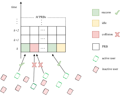
Figure 1: System Model

3 SYSTEM MODEL AND PROBLEM FORMULATION

We consider a synchronous time-slotted wireless network with a set $\mathcal{N}=\{1,\dotso,N\}$ of MTDs, a set $\mathcal{M}=\{1,\dotso,M\}$ of shared orthogonal PRBs and a receiver as shown in Fig. 1. The physical time is divided into slots, each of duration $1$ and the slot index is $k\in\mathbb{N}$. At each time slot, we assume that only $\mathcal{N}_{a}\subseteq\mathcal{N}$ devices are active and the activity pattern follows a random process. Each active MTD transmits over the shared PRBs in a grant-free manner. At each time slot $k$, an MTD can transmit only one packet and it can transmit it only over one resource $m\in\mathcal{M}$. The MTDs are assumed to have perfect synchronization. Moreover, each MTD is equipped with a buffer to store the packets in its queue and each device $n$ can only store at most one packet. The buffer state at time $k$ is defined as $B_{n}(k)\in\{0,1\}$, where $B_{n}(k)=1$ if there is a packet in the buffer and it is $0$ otherwise. If the buffer $B_{n}(k)$ is full, new packets arriving at device $n$ are discarded and are considered lost. Each device becomes active whenever a packet is generated at the device following one of the traffic arrival models given in Section 4. At each time slot $k$, MTD $n$ takes an action

$$A_{n}(k)\in\mathcal{A}=\{0,1,\dotso,M\},$$ (1)

where $A_{n}(k)=0$ corresponds to the event when user $n$ chooses to not transmit and $A_{n}(k)=m$ corresponds to the event when user $n$ transmits a single packet on channel $m$ for $1\leq m\leq M$. If only one user transmits on the channel $m$ in a given time slot $k$, the transmission is successful, whereas a collision event happens if two or more devices transmit in the same time slot. The collided packets are discarded and need to be retransmitted until they are successfully received at the receiver.

For feedback, we consider a broadcast feedback signal $F(k)$ from the receiver that is common to all the devices. Formally, we define

$$F(k)=\{F_{1}(k),\dotso,F_{M}(k)\},$$ (2)

and $F_{m}(k)$ stands for the feedback corresponding to the channel $m$ and for each time slot $k$, it is defined as

$$F_{m}(k) =\begin{cases}1&\text{if success at time slot $k$}\\ 0&\text{otherwise}\\ \end{cases}$$ (3)

Let us define the binary set $\mathcal{B}=\{0,1\}$. We define success and collision event for user $n$ as a function of the feedback $F_{m}(k)$ and $A_{n}(k)$, i.e., $g:(F_{m}(k),A_{n}(k))\mapsto G_{n,m}(k)$, and $C_{n,m}(k)$, where $G_{n,m}(k)\in\mathcal{B}$ and $C_{n,m}(k)\in\mathcal{B}$ are the success and collision event for the device $n$ respectively, and they are locally computed by each device. Formally, we define the success event for user $n$ and $\forall m\in\mathcal{M}$ as,

$$G_{n,m}(k) =\begin{cases}1&\text{if $A_{n}(k)=m$ and $F_{m}(k)=1$}\\ 0&\text{otherwise,}\end{cases}$$ (4)

and the collision event as,

$$C_{n,m}(k) =\begin{cases}1&\text{if $A_{n}(k)=m$ and $F_{m}(k)=0$}\\ 0&\text{otherwise}.\end{cases}$$ (5)

Since each device can only transmit on one resource at each time slot, the indicator whether the transmission on any resource for the device $n$ has been successful or not, can be written as $G_{n}(k)=\sum_{m}G_{n,m}(k)\in\{0,1\}$ and similarly for collision we can write $C_{n}(k)=\sum_{m}C_{n,m}(k)\in\{0,1\}$.

Furthermore, we can define matrices with $n$ rows and $m$ columns for success and collision events respectively as,

$$\boldsymbol{G}=\big{(}G_{n,m}\big{)}\in\mathcal{B}^{n\times m},$$ (6)

and

$$\boldsymbol{C}=\big{(}C_{n,m}\big{)}\in\mathcal{B}^{n\times m}.$$ (7)

We assume that each user keeps a record of its previous actions, feedback and its current buffer state $B_{n}(k)$ up to $h$ past instants, where we refer to $h$ as the history length. Therefore, the tuple

$$S_{n}(k)=\big{(}A_{n}(k-h),\dotso,A_{n}(k-1), F(k-h),\dotso,$$ (8)

$$F(k-1),B_{n}(k)\big{)}$$

is referred to as the local history or the state of user $n$ at time $k$, and $S(k)=\big{(}S_{1}(k),\dotsc,S_{N}(k)\big{)}$ is the global history of the system.

The feedback signal $F(k)$ is only recorded by the devices that are active at time $k-1$. If a new device becomes active at time $k$, its state is initialized with $A_{n}(k-1)=0$, and $F_{m}(k-1)=0,\forall m\in\mathcal{A}$ for its local history $S_{n}(k)$. The memory is initialized with zero values. Moreover, we set zero values for the time a device has been inactive if the time of inactivity is smaller than the history size.

Definition 1

A policy or access scheme of user $n$ at time slot $k$, is a mapping from $S_{n}(k)$ to a conditional probability mass function $\pi_{n}(\cdot|S_{n}(k))$ over the action space $\{0,1\}$. We consider a distributed setting in which there is no coordination or message exchange between users for the channel access. Each new action $A_{n}(k)\in\{0,1\}$ is drawn at random from $\pi_{n}(\cdot|S_{n}(k))$ as follows:

$$\mathrm{Pr}\bigl{\{}A_{n}(k)=a\bigm{|}S_{n}(k)=s\bigr{\}}=\pi_{n}(a|s).$$ (9)

We are interested in developing a distributed transmission policy for slotted RA that can effectively adapt to changes in the traffic arrivals and provide better performance in terms of throughput, latency and fairness than the baseline reference schemes. We consider EB policies as our baseline schemes. More specifically, we use BEB when the value of backoff factor is $2$, which has been used in IEEE 802.11 and IEEE 802.3 standards.

3.1 PERFORMANCE METRICS

3.1.1 Throughput

The channel throughput is defined as the average number of packets that are successfully transmitted from all the devices divided by the total number of PRBs, over a time window of size $K$. For the finite time horizon $K$ and for $M$ orthogonal resources, the average throughput of the system is defined as

$$T=\frac{1}{MK}\sum_{k=1}^{K}\sum_{m=1}^{M}\sum_{n\in\mathcal{N}}G_{n,m}(k).$$ (10)

where $G_{n,m}(k)$ refers to the success event over channel $m$ and $T\in[0,1]$.

3.1.2 Age of Packets

The age of packet (AoP) of device $n$, denoted as $w_{n}(k)$, grows linearly with time if a packet stays in the buffer of the device, and it is reset to $0$ if the packet is transmitted successfully. Specifically, we assume that $w_{n}(1)=0$, and the AoP $w_{n}(k)$ evolves over time as follows:

$$w_{n}(k) =\begin{cases}0&\text{if }B_{n}(k)=0\\ w_{n}(k-1)+1&\text{otherwise.}\end{cases}$$ (11)

The average AoP for user $n$ after a time span of $K$ time slots is given by

$$\Delta_{n}=\frac{1}{K}\sum_{k=1}^{K}w_{n}(k)$$ (12)

and the average AoP of the overall system by $\Delta=\frac{1}{N}\sum_{n}\Delta_{n}$. Since techniques such as EB incur capture effect [8] where a transmitting device keeps transmitting on the channel for some time, introducing short-term unfairness. In this work, we use the average AoP to measure fairness as well as the average delay budget of the packets. A higher AoP means the scheme is more unfair and has the higher delay and vice versa.

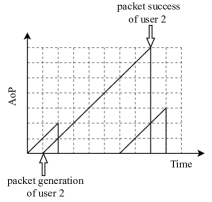
(a) Unfair Scheme

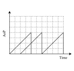
(b) Fair Scheme

Figure 2: An example of using AoP for fairness.

To illustrate the concept of fairness with AoP, let us consider an example of $3$ users where each user generates a single packet that is successfully transmitted within $K=10$ time slots as depicted in Fig. 2. The average delay (number of time slots taken by each user to transmit their packet is same for both fair and unfair schemes, which is $4$ time slots. However, the scheme shown in Fig. 2(a) is clearly not fair since user $2$ takes much more time slots to send its packet as compared to the other two users. This short-term unfairness can be captured with the average AoP and we see that the average for the scheme in Fig. 2(a) is higher i.e., $1.23$) than the one shown in Fig. 2(b) which is $1.00$.

4 TRAFFIC MODELS

4.1 REGULAR TRAFFIC MODEL

In traditional RA schemes, the activation of MTDs and the traffic arrival for each user is usually modeled by an independent process. We call such traffic arrival as regular traffic arrival. Each device follows independent Bernoulli process with average arrival rate $\lambda_{n}$ to generate packets in regular traffic model. The average arrival rate for the system can then be written as

$$\lambda=\sum_{n}\lambda_{n}$$ (13)

However, for machine-type communication (MTC), it is highly likely that some devices are correlated in terms of activation, i.e., some devices observe the same physical phenomenon and activate together. For instance, in industrial fault detection or fleet management, some MTDs are highly likely to transmit at the same time due to the activation of certain event. For intance, in flood or quake detection or land sliding, there is a high probability that devices closer to the event will start transmitting at once. Several recent works have used a correlated activity model to design access schemes for MTC [22, 28, 29, 30]. Therefore, the assumption of independent traffic arrival is not valid in this case. Moreover, apart from correlated ED device activity, each MTD also follows regular traffic model [31].

4.2 CORRELATED TRAFFIC MODEL

The correlated traffic model is a mix of the regular traffic and ED traffic or alarm traffic as depicted in Fig. 3. We assume that the regular traffic generation for each MTD follows an independent random process such as Bernoulli process. Similarly, the ED traffic also follows a random process on top of the regular traffic arrival process. For ED traffic, certain devices are strongly correlated in space and time and the ED traffic generation for such devices is dependent on the occurrence of an event in their vicinity. Regular traffic arrival and ED traffic arrival processes are independent of each other.

To formulate this behaviour, we assume that $N$ MTDs are uniformly distributed in a given area. Each MTD can either be in a regular state or alarm state, when active. We consider $L$ event epicentres that are scattered randomly and independently across the given area. The location of the devices is represented by $\mathbf{x}\in\mathbb{R}^{2}$ and the location of the epicenter of the events is denoted by $\mathbf{y}\in\mathbb{R}^{2}$. We assume that all MTDs are stationary and fixed to their locations or exhibit very low mobility.

Let $E_{\mathbf{x}\mathbf{y}}$ denote the event when a device $n\in\mathcal{N}$ at location $\mathbf{x}$ is triggered into alarm or ED mode by the activation of an event with its epicenter at location $\mathbf{y}$. Let $\bar{E}_{\mathbf{x}\mathbf{y}}$ be the complement of $E_{\mathbf{x}\mathbf{y}}$ and $p_{\mathbf{x}\mathbf{y}}$ denotes the probability of a device $n$ at location $\mathbf{x}$ being triggered into alarm mode by the activation of event at location $\mathbf{y}$. Moreover, we define the probability of device at location $\mathbf{x}$ being in ED mode is $p_{\mathbf{x}}$. We write,

$$p_{\mathbf{x}} =\mathrm{Pr}\big{[}\text{At least one event triggers \lx@glossaries@gls@link{acronym}{mtd}{\leavevmode MTD} at }\mathbf{x}\big{]}$$

$$=1-\mathrm{Pr}\big{[}\text{No event triggers \lx@glossaries@gls@link{acronym}{mtd}{\leavevmode MTD} at }\mathbf{x}\big{]}$$

$$=1-\prod_{\mathbf{y}\in\mathcal{L}}\mathrm{Pr}\big{[}\bar{E}_{\mathbf{x}\mathbf{y}}\big{]}$$ (14)

$$=1-\prod_{\mathbf{y}\in\mathcal{L}}(1-p_{\mathbf{x}\mathbf{y}}),$$ (15)

where we have assumed that events are triggered independently of each other.

Therefore, for the correlated traffic arrival model, each MTD can either be at alarm (ED) state or regular state for a given time slot $k$. We denote by $V_{\mathbf{x}}$ the state of device at location $\mathbf{x}$ and we model the states at each time slot $k$ by i.i.d Bernoulli random variable as,

$$V_{\mathbf{x}}(k)=\begin{cases}\text{Regular with prob. }1-p_{\mathbf{x}}\\ \text{Alarm with prob. }p_{\mathbf{x}}\end{cases}$$ (16)

Moreover, we define with $p$ the probability of an event being active at location $\mathbf{y}$. We assume that each event at epicenter $\mathbf{y}$ triggers a subset $\mathcal{N}_{\mathbf{y}}\subseteq\{1,\dotsc,N\}$ of devices. The probability of a device $n$ going into alarm mode depends on the distance of the device from the epicenter $\mathbf{y}$ of the event. Furthermore, each MTD $n$ can sense and report multiple events but at any given time, we assume that it can report about only one event. The MTDs are unaware of the actions, and events sensed by other devices.

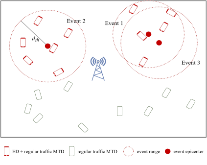
Figure 3: MTC Network depicting $N=20$ MTDs uniformly distributed in a rectangular area with $L=3$ event epicenters. MTDs follow regular traffic and those within the range of the event epicenter follow both regular and ED traffic.

Table 1: Suitability of some popular MARL for designing RA schemes for MTC systems

MARL Algorithm	Features	Limitations
DQN [32] and variants	Can be used as independent Q learning (IQL) or centralized learning using PS by extending single agent network to multiple agent.	Has convergence issues and it is nearly impossible to learn optimal policy for a large number of agents with PS.
MADDPG [33] MAPPO [34]	• They have a shared critic and local actors. • MAPPO is on-policy and MADDPG is off-policy for CTDE method. • Both circumvent the challenge of non-Markovian and non-stationary environments during learning. • Stabilize learning, due to reduced variance in the value function estimates.	• Need centralized critic which is not scalable to a large number of agents. • The state-space dimensionality grows exponentially for the critic as the number of agents increases. • Most critically, the accumulated noises by the exploratory actions of other agents make the Q-function learning no longer feasible [35].
COMA [36]	• Tackles the credit assignment problem. • Calculates the advantage function which is able to marginalize a single agent’s actions while keeping others fixed.
QMIX [35] VDN [37]	• Lie between COMA and IQL. • Better scalability than centralized critic methods. • Each agent has its own network and then mixing network takes the Q-values of agents to measure $Q_{tot}$. • QMIX uses NNs to make the function monotonic whilst VDN is the linear combination of the Q values of each agent. • Both of them make use of RNNs.	• Scalability to a massive number of agents. • Different policy for each agent and it can also be applied to homogeneous agents with PS. • The information might be lost in this way of centralized training. • It is not sure whether the training with PS without using agent IDs will result in better policy than DQN or not.
Mean Field MARL (MF-MARL) [38]	Good scalability results and and it considers the effects of neighbouring agents for each agent to estimate its value function	Requires communication between agents; each agent has its own policy to learn.
Multi-Actor-Attention-Critic (MAAC) [39]	Uses attention mechanism to incorporate the effects of important agents whom actions are given more consideration than others	Requires communication among agents, scales better than MADDPG but their results are only for a small number agents.
Soft Actor Critic [40]	• Extension of AC methods. Uses the notion of entropy to encourage exploration and to avoid converging to non-optimal policies. • Can be used for multiagent system with PS, local actors and local critics.	• Has convergence issues just like DQN. • The performance is not known with centralized training, i.e., centralized critic and centralized actor, an extension of single agent system just like DQN.

5 SUITABILITY OF MARL FOR RA SCHEME DESIGN

To design a RA policy for the multiuser MTC environment, it is important to consider the suitability of MARL algorithms in general for scalability and in particular for the specific characteristics of MTC system. There exists a large body of the literature for medium access using RL in wireless networks but only a few address the issues of scalability (e.g., [41] and our recent work [24]). The distributed multiple schemes designed with MARL do have scalability challenges and this is even further exacerbated by the limitations of the mMTC. The MTC system presents the following challenges for MARL algorithms in designing a distributed RA policy:

1. Since the MTDs are low-powered and low-complexity devices that are battery-operated, it is not feasible to perform learning on the devices and therefore, centralized training and decentralized execution (CTDE)method is required for learning.

2. Usually, PS method is used for homogeneous agents, and each agent’s ID is used in the observation (state) vector to distinguish between agents. The homogeneous agents are those that have the same state-space and action-space. In our system model, since the devices have variable sleep cycles and they should be able to join/leave the network, it is not feasible to use agent identification. Therefore, we require each agent to have a single policy using PS but at the same time, without using agent IDs.

3. Any communication to exchange channel or device information between MTDs is not energy efficient as it will drain the battery of the devices. Therefore, the devices do not communicate with each other and they do not know the actions taken by the other devices.

In Table 1, we provide the comparison of some popular MARL algorithms and their suitability to the proposed system model. Even though there are several MARL algorithms found in the literature, we have given the comparison of some well-known algorithms that employ the CTDE method to learn policies. The aim of this comparison is not to provide an exhaustive survey of MARL algorithms but to make a case of using a specific algorithm over the others for the proposed system model. Interested readers are referred to [42], a recent review paper of different MARL algorithms addressing scalability challenges. Moreover, we are focusing on DRL algorithms only.

Standard DQN [32] and actor-critic algorithms are extended to multiple agents using PS for homogeneous agents in [43]. This method scales well to a large number of agents but it does not exploit any advantages of centralisation. Moreover, without using IDs of agents and without any cooperation between agents, we have observed in our simulations that these algorithms are not able provide better policies and they have convergence issues. However, this might be the issue for most of the centralized approaches. Our recent works [23] and [24] use the DQN with PS and in [24], we provided results for up to 500 devices for the bursty traffic. Similarly, just like the DQN can be extended to multiple agents using PS, one can also use Soft Actor Critic method [40] with a local actor and local critic that is shared among all users, where users’ individual observation is used to update the actor and critic at each time step for all the users.

Other popular choices for MARL are multi-agent deep deterministic policy gradient (MADDPG) [33] and the recently proposed multi-agent proximal policy optimization (MAPPO) [34]. In both MADDPG and MAPPO, the critic network has a global view of the system, which is only applied during the training phase and actor networks are employed for each agent. A major bottleneck of these algorithms is the scalability due to the shared critic network, even if the PS is considered. Since the shared critic network has the observation space of all the agents, the size of the observation space will grow exponentially with the number of agents. Moreover, in a network where the number of agents changes with time, it is inefficient to use the state-space of all agents at the centralized critic. counterfactual multi-agent policy gradients (COMA) [36] has a similar issue for scaling to a higher number of agents because a shared critic is used in it as well, just like MADDPG and MAPPO.

Some algorithms such as mean field MARL (MF-MARL) [38] and multi-actor-attention critic (MAAC) [39] show good scalability results but the major issue in these algorithms is that they require communication between the agents, which is not practical for our system model. Furthermore, the results for these algorithms are shown for a moderate number agents.

VDN [37] and QMIX [35] are both for cooperative multi-agent learning in which joint action-values $Q_{tot}$ are estimated from Q-values of individual agents that condition only on local observations. One of the main differences between these algorithms is that in VDN, the $Q_{tot}$ is calculated as a linear combination of the Q-values of each agent, while QMIX employs a network that can compute $Q_{tot}$ as complex non-linear combination of individual Q-values. This way of learning also provides better scalability as compared to MADDPG and MAPPO. QTRAN [44] improves upon both VDN and QMIX and provides more general form of factorization but it falls under the same category as VDN and QMIX. For these reasons, we will focus on the VDN and QMIX algorithms in our simulations.

6 RL ENVIRONMENT AND MARL ALGORITHMS

6.1 THE ENVIRONMENT

We consider shared PRBs where each agent interacts with the resources by taking an action and receiving a common feedback $F(k)$ as observation. The reward $R_{n}(k)$ is then calculated by each agent. The action space of each agent is $\mathcal{A}$ and each device can either transmit on channel $m$, i.e., $A_{n}(k)=m$ or it can stay silent, i.e., $A_{n}(k)=0$. The state of each device is the history tuple $S_{n}(k)$ defined in (8). Let $R_{n}(k)\in\mathbb{R}$ be the immediate reward that user $n$ obtains at the end of time slot $k$. The reward depends on the agent $n$ action $A_{n}(k)$ and other agents’ actions $A_{n^{\prime}}(k)$, $n^{\prime}\neq n$. The accumulated discounted reward for user $n$ is defined as

$$\mathcal{R}_{n}(k)=\sum\limits_{k^{\prime}=0}^{\infty}\gamma^{k^{\prime}}R_{n}(k+k^{\prime}+1),$$ (17)

where $\gamma\in[0,1)$ is a discount factor. The reward function to maximize the packet success rate is defined as,

$$R_{n}(k)=\sum_{i=1}^{N}\sum_{m=1}^{M} G_{i,m}(k),\quad\forall i\in\mathcal{N},\forall m\in\mathcal{M}$$ (18)

The summation sign over agents shows that the reward is global, i.e., all agents receive the same reward, which indicates that the agents are fully cooperative. The environment is partially observable as each agent is unaware of the actions taken by the other user,

At each time slot $k$, each agent $n$ obtains the feedback $F(k)$ from the receiver, updates its history and then feeds $S_{n}(k)$ to the proposed algorithm, whose output are the Q-values for all the available actions. Each agent $n$ follows the policy $\pi$ by drawing an action $A_{n}(k)$ from the following Boltzmann distribution,

$$\pi(a|s) =\frac{e^{Q(a,s)/\tau}}{\sum\nolimits_{\tilde{a}\in\{0,\dots,M\}}e^{Q(\tilde{a},s)/\tau}},\qquad\forall a\in\{0,\dots,M\},$$ (19)

where $0<\tau<\infty$ is the temperature parameter which is used for exploration. We decrease the value of $\tau$ to $0$ gradually to make the agent more greedy.s

6.2 DEEP Q-NETWORK (DQN)

DQN represents the action-value function using a neural network that are characterized by parameter $\theta$. In double DQN, a target network is also used which is parameterized by $\theta^{-}$ that are periodically copied from $\theta$ during training. The DQN and its variants use a replay buffer to store the transitions $(s,a,r,s^{\prime})$, where $s$ is the actual state, $s^{\prime}$ is the next state that is observed after taking action $a$ and receiving reward $r$. The learning updates are applied on the experience samples $(s,a,r,s^{\prime})\sim U(\mathcal{D})$, that are drawn at random with uniform distribution as mini-batches of size $z$ from $\mathcal{D}$ and by minimizing the following loss function,

$$L(\theta)=\sum_{i=1}^{z}\Big{[}\big{(}y_{i}^{DQN} -Q(a_{i},s_{i};\theta_{i})\big{)}^{2}\Big{]},$$ (20)

where $y_{i}^{DQN}=r+\gamma\max_{a^{\prime}}Q(a^{\prime},s^{\prime};\theta_{i}^{-})$ is the target value for the $i^{\text{th}}$ iteration.

Since the environment is partially observable, the agents can benefit from using RNN such as gated recurrent unit (GRU) that can facilitate learning from previous history. A DQN making use of RNN is referred to as DRQN.

6.3 VALUE DECOMPOSITION NETWORKS (VDN)

VDN [37] take advantage of centralization and aim to learn the joint action value function $Q_{tot}(\boldsymbol{s},\boldsymbol{a})$, a linear value decomposition from the team reward signal, where $\boldsymbol{s}$ is the joint observation of the agents and $\boldsymbol{a}$ is the joint action of agents. The VDN algorithm decomposes the $Q_{tot}$ as the linear combination of the individual Q-values of each agent, i.e.,

$$Q_{tot}(\boldsymbol{a},\boldsymbol{s})\approx\sum_{n=1}^{N}Q(a_{n},s_{n};\theta_{n}),$$ (21)

The loss function of the VDN algorithm can be calculated in the same way as DQN, i.e.,

$$L(\theta)=\sum_{i=1}^{z}\Big{[}\big{(}y_{i}^{tot} -Q_{tot}(\boldsymbol{a},\boldsymbol{s};\theta_{i})\big{)}^{2}\Big{]},$$ (22)

where

$$y_{i}^{tot}=r+\gamma\max_{\boldsymbol{a}^{\prime}}Q(\boldsymbol{a}^{\prime},\boldsymbol{s}^{\prime};\theta_{i}^{-})$$ (23)

is the target value for the iteration $i$.

In this way, each agent performs an action selection locally based on its own learned Q-value in a decentralized manner. Moreover, the VDN method employs RNN or DRQN to calculate Q-values for each agent.

6.4 QMIX

The QMIX [35] algorithm improves the VDN and it can represents much richer class of action-value functions. QMIX applies the following constraint on the relationship of $Q_{tot}$ and each individual action-value $Q_{a}$,

$$\frac{\partial Q_{tot}}{\partial Q_{a}}\geq 0\quad\forall a,$$ (24)

to ensure that mixing network has positive weights. Intuitively, it shows that if the weights of individual value function $Q_{a}$ are negative, less weightage is given to that agent for cooperation. Moreover, as opposed to VDN, $Q_{tot}$ is calculated in a complex non-linear way. QMIX uses a separate feed-forward neural network as a mixing network that takes individual agents’ outputs and mixes them monotonically to produce $Q_{tot}$ to enforce the constraint in (24) [35]. The weights of the mixing network are produced by a separate hypernetwork to ensure that they are non-negative. The loss function is calculated in the same way as given in (22).

Algorithm 1 Training Phase of the Proposed Algorithm

  

  Define $N,\tau,\gamma\in[0,1],\lambda_{n},\forall n\in\mathcal{N},h$ and $K$

  Initialize $S_{n}=0,B_{n}=0,\forall n\in\mathcal{N}$

       for each episode do

           $\textbf{for}\text{ each time slot }k=1,\dots,K\textbf{ do}$

                Generate traffic for all MTDs, i.e., $\tilde{B}_{n}\sim$

                $Bernoulli(\lambda_{n})$ for regular traffic, and $\tilde{B}_{n}\sim$

                $Bernoulli(p)$ for ED traffic, $\forall n\in\mathcal{N}$

                Update buffer $B_{n}=\min(1,\tilde{B}_{n})$

               $\textbf{for}\text{ each agent/\lx@glossaries@gls@link{acronym}{mtd}{\leavevmode MTD}}n=1,\dots,N\textbf{ do}$

                    Observe input $S_{n}$ and feed it to DRQN

                    Generate the estimate of $Q_{a},\forall a\in\mathcal{A}$

                    Choose action according to (19)

                    Receive feedback $F(k)$ from the receiver

                    Obtain reward $R_{n}$ according to (18)

                    Update buffer $B_{n}$

                    Observe the next state $S_{n}$

                $\mathbf{end}$

                Store $(S,\mathbf{A},\mathbf{R},S^{\prime})$ in the replay buffer $\mathcal{D}$,

                where $\mathbf{A}=(a_{1},\dots,a_{N})$, $\mathbf{R}=(R_{1},\dots,R_{N})$

                Set $S\leftarrow S^{\prime}$

                Sample a minibatch $(S^{i},\mathbf{A}^{i},\mathbf{R}^{i},S^{\prime i})$ from $\mathcal{D}$

                Calculate $y^{tot}$ using (23)

                $\mathbf{if}$ mixer $=$ VDN:

                    Calculate $Q_{tot}$ using (21)

                $\mathbf{elseif}$ mixer $=$ QMIX:

                    Calculate $Q_{tot}$ using QMIXer [35]

                $\mathbf{for}$ every $K^{\theta}$ time slots:

                    Update $\theta^{-}\leftarrow\theta$

                $\mathbf{for}$ every $K^{\beta}$ time slots:

                    Update $\beta$

            $\mathbf{end}$

        $\mathbf{end}$

Table 2: Simulation Parameters

Parameter	Value
$\tau$	200 – 0.1
$\lambda_{n}$	0.3 (regular) and 0.015 (correlated)
Total Episodes	$60$
History size $h$	5 if RNN else 1
Learning rate	$10^{-4}$
Batch size	32
$d_{th}$	0.3

7 SIMULATION RESULTS AND DISCUSSION

In the following experiments, we use the VDN [37] method to learn RA policies for different values of $N$ and $M$. We use the neural network with two layers of size $256$ and $64$ units before the final layer of size $M$, and when RNN is used, a GRU layer of $64$ neurons is added after the first layer. The parameters used during the training of the network are presented in Table 2. In all the experiments, we use experience replay to accumulate each agent’s experience and the learning is performed with CTDE method. An agent’s ID is one-hot encoded vector that is appended with the observation $S_{n}(k)$ of each agent. We will first provide results for regular traffic in which we also compare the results for different MARL algorithms such as QMIX and DRQN with VDN and then we present our results for the correlated traffic arrival model.

7.1 RESULTS FOR REGULAR TRAFFIC

For regular traffic, we employ two ways of training all algorithms: (i) using agents’ IDs in the observation vector, which is a common way of training for CTDE, and (ii) without using them. We denote IDs $=0$ as the case when agent IDs are not used and IDs $=1$ as the case when we incorporate agent IDs in the observation space.

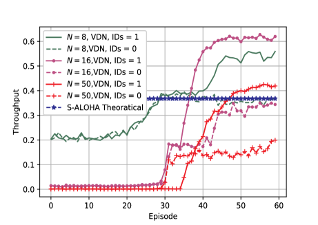
Figure 4: Average throughput during training with VDN algorithm for different values of $N$ and to compare the cases when using IDs and not using IDs. The results are for $\lambda_{n}=0.3$ and $(K,N)=(2000,8)$, $(K,N)=(3000,16)$ and $(K,N)=(5000,50)$.

Table 3: Average throughput and average AoP values for the proposed algorithm compared to the BEB for the learned policies shown in Fig. 4.

		Av. Throughput			Av. AoP
$N$	$M$	VDN IDs=1	VDN IDs=0	BEB	VDN IDs=1	VDN IDs=0	BEB
$8$	2	$0.56$	$0.40$	$0.37$	$625.7$	$5.5$	$162.2$
$16$	2	$0.54$	$0.386$	$0.372$	$1480.4$	$29.8$	$519.3$
$50$	5	$0.44$	$0.25$	$0.36$	$1561.3$	$44.1$	$1095.1$

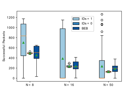
(a) Packets success distribution

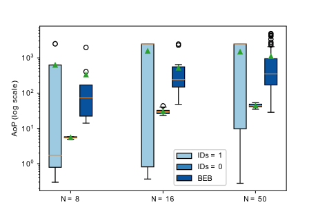
(b) AoP distribution

Figure 5: Distribution of successful packets and AoP among MTDs for $N=\{8,16,50\}$ and $\lambda_{n}=0.3$. We used VDN for both IDs $=1$ and IDs $=0$ cases. All cases tested for $K=500$ time slots.

We show the results in terms of average throughput (normalized reward) and AoP. The learning process and how average throughput of the system increases for different values of $N$ is shown in Fig. 4. We use $K=2000,3000$, and $5000$ per episode during training for $N=8,16$ and $50$, respectively. We increase $K$ per episode as $N$ grows to allow better learning for each value of $N$. Moreover, $M=2$ is used to $N=8$ and $16$ and $M=5$ is used when $N=50$. The average throughput and average AoP after testing is shown in Table 3. Clearly, the case IDs $=1$ outperforms BEB, slotted ALOHA theoretical throughput (i.e., $1/e$), and the case when IDs$=0$. The case IDs $=0$ provides much lower average throughput and as the number of devices $N$ grow, the average throughput also decreases which is not surprising because agents decrease the transmit probability as $N$ grows.

Moreover, we calculate whether the learned policy is fair or not in two different ways as depicted in Fig. 5. First, we show how many packets per user have been successful as in Fig. 5(a) and the second, the AoP of individual users (which shows both packet delay and fairness) as shown in Fig. 5(b). We observe that using IDs incurs a significant unfairness among devices as a subset of MTDs are starved out and they never get a chance to send a packet. Surprisingly, no IDs case provides much better fairness among devices. It is due to the inherent way the MARL algorithms with CTDE behave, we see that the case where IDs are omitted, provides us better fairness as compared to the other case. When we use IDs in the state space, devices are only concerned about achieving a better throughput. But when we do not use IDs, there’s no such coordination that exists during the centralized training, which could allow the MTDs to come up with an unfair consensus.

To understand this, let us take the case of $N=8$. For VDN, IDs $=1$ case, it is clear that there are some devices that have sent $0$ packets and there are a few devices that have sent most of the packets ($95$^th percentile is $1070$ and $25$^th percentile is around 443). Similarly, in Fig. 5(b) for $N=8$, the average AoP value, which is the mean point and the distribution of AoP among each device shows a significant difference between $75$^th percentile ($627$) and $25$^th percentile ($0.8$). On the other hand, for VDN, IDs $=0$ case, the number of successful packets sent by each device are around the mean value ($493$) for all percentiles, i.e., $75$^th percentile is around $500$ and $25$^th percentile is around $486$. Similarly, the average AoP value as shown Fig. 5(b) and in Table 3 for VDN ID$=0$ case is much lower ($5.5$), which is the indication of fairness. Similar conclusion can be drawn for $N=16$ and $N=50$.

The case when IDs $=0$ allows agents update the policies as if it is a single agent (hence single policy). This is unlike the IDs $=1$ case in which, even if the state-space is the same for agents, they behave differently. This way we achieve better trade-off without using agent IDs, which is also scalable and allows devices to join/leave the network without identification. These plots also show that IDs $=1$ case outperforms the BEB in terms of average throughput but BEB has better average AoP than IDs $=1$ case. The average throughput of BEB technique is higher than IDs $=0$ case for higher values $N$ but no IDs case exhibits much better throughput-fairness tradeoff, as evident from average AoP values. The case where agents IDs are used is most unfair because of the reward signal that only cares about maximizing the throughput.

Obviously, one can learn a policy by designing a reward function that enforces the devices to be fair even when agent IDs are incorporated; however, such a scenario is not of our interest in this paper.

7.1.1 Comparison between VDN, QMIX and DRQN

We used VDN algorithm to learn RA schemes for IDs and no IDs cases. In Fig. 6, we compare the performance of VDN with QMIX and DRQN for $N=8$ and $M=2$. Both VDN and QMIX use mixer networks to calculate the total Q-value $Q_{tot}$ and exploit the benefits of centralized learning. However, DRQN does not take any such advantage of centralized training. For this reason, we can see that both QMIX and VDN algorithms learn a policy that maximizes the throughput for the case when agent IDs are incorporated (IDs $=1$) and QMIX outperforms VDN. Interestingly, the DRQN learns only a slightly better policy when IDs $=1$ as compared to the case when agent IDs $=0$, again, due to the major difference that it doesn’t take any advantage of centralization as opposed to the VDN and QMIX. However, in Fig. 7, we can clearly see that QMIX and VDN learn a policy that is unfair when IDs $=1$, VDN being more unfair than QMIX. On the other hand, the DRQN for this case has lower AoP and relatively much fairer policy than VDN and QMIX. It does not imply that DRQN is a better algorithm than VDN and QMIX. In fact, QMIX outperforms VDN and both of them outperform DRQN as far as the objective (maximizing throughput) is concerned. Another interesting observation is that the learned policies are very similar between all the algorithms for IDs $=0$ case and it is evident from both Fig. 6 and Fig. 7. They are fair but it seems that exploiting centralization advantages without using agent IDs does not provide significant improvements.

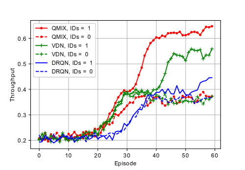
Figure 6: Average throughput comparison of different MARL algorithms during training, for $N=8$ and $\lambda_{n}=0.3$.

Figure 7: The AoP comparison among MTDs for different MARL algorithms for $N=8$ and $\lambda_{n}=0.3$

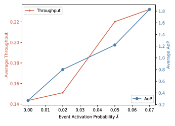
Figure 8: Average throughput and average AoP for different values of $\bar{\lambda}$ when $N=20$, $L=3$ and $\lambda=0.3$

7.2 RESULTS FOR CORRELATED TRAFFIC

In this work, we are interested in designing an access policy for the MTDs deployed in an area, and whenever an event $l$ happens, the MTDs in the vicinity of the event or the MTDs closer to the epicenter of the event become active in a correlated manner. To model this, we calculate the probability of a device at location $\mathbf{x}$ becoming active due to the event happening at epicenter $\mathbf{y}$ as $p_{\mathbf{x}\mathbf{y}}$ in the following way:

$$p_{\mathbf{x}\mathbf{y}}=\begin{cases}1\quad\text{if }d_{\mathbf{x}\mathbf{y}}\leq d_{th}\\ 0\quad\text{otherwise},\end{cases}$$ (25)

where $d_{\mathbf{x}\mathbf{y}}=\lVert\mathbf{x}-\mathbf{y}\rVert$ and $d_{th}$ is the threshold distance. We assume that the events are atomic in nature, i.e., if an event becomes active in time slot $k$, it activates MTDs within $d_{th}$. We assume that each MTD activated by an event has one packet each to transmit and the MTDs remain active until their packets are successfully transmitted.

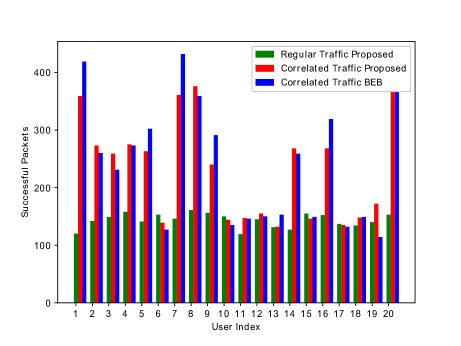
(a) Successful packets per user

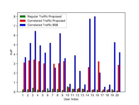
(b) AoP per user

Figure 9: The comparison of successful packets per user and AoP of each user for ED traffic model for $(K,N)=(10000,20)$, $L=3$, $\lambda=0.3$ and $\bar{\lambda}=0.07$.

For correlated traffic arrival, we consider the example as shown in Fig. 3, in which $N=20$ MTDs are randomly distributed in rectangular area. The MTDs follow Bernoulli process with average arrival rate $\lambda=0.3$ for regular traffic. We consider $L=3$ event epicenters and MTDs belonging to each epicenter are given in 5. The events become active following another independent Bernoulli process with average event activation probability given by $\bar{\lambda}$ such that $p=\bar{\lambda}/L$. We train and test for different values of $\bar{\lambda}$ as shown in Table 4. The training for each $\bar{\lambda}$ is performed over $60$ episodes and $K=2000$ time slots per episode.

Since we want to learn the same policy for each agent, we do not use agent IDs for correlated traffic arrivals case and we only consider VDN IDs $=0$ case since have seen that VDN performs better as compared to the QMIX and DRQN, Moreover, we do not consider whether events-driven traffic has any priority over regular traffic. All events are of the same nature and the same reward function as the regular traffic is used. Fig. 8 shows the average throughput and average AoP for different values of $\bar{\lambda}$. The value $\bar{\lambda}=0$ means that there is only regular traffic and we see in Fig. 8 that as the $\bar{\lambda}$ increases, the average throughput and average AoP both increase, which is natural because when there is more traffic, there are more packets being successful but require more time to be transmitted.

Table 4: Number of times each event was activated for $K=10,000$ time slots for different event activation probabilities $\bar{\lambda}$.

$\bar{\lambda}$	Event 1	Event 2	Event 3
$0.02$	63	61	59
$0.05$	170	170	169
$0.07$	243	226	241

Table 5: MTDs reporting the events as in Fig. 3

Event #	MTDs Index
$1$	$1,7,8,16,20$
$2$	$2,3,4,5,9,14$
$3$	$1,7,8,20$

By further zooming in on individual MTDs, we want to observe how each MTD is behaving in correlated traffic scenario. In this case, we do not incorporate agent IDs in the state-space of agents. Fig. 9 shows successful number of packets and AoP per device and we compare the correlated traffic with regular traffic arrival scenario. Clearly, only users that are involved in reporting any event have higher throughput as well as higher AoP. Obviously, when few users become active together, they will take more time to resolve collision and to send their packets successfully. The reason to show these plots is that the RL-based algorithms adapt to the traffic changes as the devices that are not involved in reporting any events have similar AoP and packet success rate to the regular traffic case, and only the MTDs belonging to events change their policies. The baseline BEB does not really adapt or care whether the devices are involved in events. The throughput is high for BEB for devices that are receiving more packets which is not surprising but if we look at the AoP plot in Fig. 9(b), there are devices that are not involved in reporting any events but they have higher AoP for BEB as opposed to the proposed algorithm.

7.3 SCALABILITY AND ROBUSTNESS ANALYSIS

We compare the learned policies of VDN, QMIX and DRQN for no IDs case and show how robust the policy learned is by each algorithm if we scale it for a higher number of devices. The performance of each algorithm in terms of average throughput is shown in Fig. 10. We denote with $N_{\mathrm{tr}}$ the number of devices during training, and the number of devices for testing is denoted by $N_{\mathrm{test}}$. The average arrival rate of the system is $\lambda=0.3$. The results are simulated for $3$ different random seeds and the best performances are shown in Fig. 10.

We show that the VDN has more robust policy than both QMIX and DRQN. For $\lambda=0.3$, the policy learned for $N_{\mathrm{tr}}=4$ performs the same $N_{\mathrm{test}}={4,8,16}$ and the throughput starts dropping after that. It is because the policy learned for $N_{\mathrm{tr}}=4$ has higher $\lambda_{n}=\lambda/N_{\mathrm{tr}}$ and as the number of devices grow, the collisions are not resolved and hence the average throughput drops to almost $0$. On the other hand, the policy learned for a relatively higher number of devices such as $N_{\mathrm{tr}}=16$ is robust for the number of devices less than $N_{\mathrm{tr}}$ and also scales for a large number of devices.

Intuitively, for instance, when $N_{\mathrm{tr}}=4$ and $\lambda=0.3$, then $\lambda_{n}$ for smaller $N_{\mathrm{tr}}$ has higher arrival rate or in other words, the MTDs observe packet arrival more frequently than $\lambda_{n}$ for larger $N_{\mathrm{tr}}$ and therefore, devices learn to be more aggressive in terms of their transmissions to empty their buffers and such policy does not perform well for a very large number of devices.

Furthermore, the policy of QMIX has worse performance as compared to both VDN and DRQN. We can also observe that QMIX without incorporating agent IDs is not as effective and not as robust as compared to the VDN.

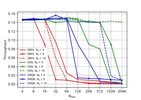
Figure 10: Average Throughput performance of the learned policy for $\lambda=0.3$ for different $N_{\mathrm{tr}}$ and tested for $N_{\mathrm{test}}$.

8 CONCLUSION AND FUTURE WORK

In this paper, we have proposed MARL-based RA schemes for multi-user multi-channel mMTC network. We have used the broadcast feedback commonly received by all the MTDs. We demonstrated that incorporating agents IDs is not suitable for mMTC systems, as we aim to design a fair and a scalable scheme. We have shown that even when the optimization objective is to maximize throughput, not incorporating agent IDs provides a fair use of resources by each agent and, thus, results in a better throughput-fairness tradeoff as compared to the BEB scheme and when IDs are used. This is supported by our analysis of successful packet distribution per user and also through average AoP. We presented the scalability analysis of the proposed algorithms where we omit agent IDs for learning and we conclude that our system scales well for lower average arrival rates and that the learned policy is more robust for VDN as compared to the QMIX and DRQN. Moreover, we have presented the suitability of several popular MARL algorithms and have shown that the VDN and QMIX take advantage of centralization and they are better suited for designing RA schemes for mMTC. We have demonstrated that RL-based algorithms can adapt to changes in traffic, whereas EB schemes are not aware of such changes. We have used a correlated traffic arrival model along with the regular traffic, for which we show that the users learn the correlation and adapt to changes in the traffic.

For the correlated traffic, we have assumed that all the events are of the same nature and they have the same priority. Future works could consider prioritizing events to learn a scheme where the devices with high priority send their packets with low latency. Moreover, one can use agent IDs for a system where the devices are fixed and known, we can design a reward that is fair and that exploits correlation between devices even better. Furthermore, whilst omitting IDs make the scheme fair, the system throughput goes to zero as for a large number of devices; therefore, there may be a need to design algorithms with some coordination among devices or a group of devices.

[] MUHAMMAD A. JADOON (Student Member, IEEE) is a research assistant at the Centre Tecnològic de Telecomunicacions de Catalunya (CTTC) and an early stage researcher (ESR) of ITN Windmill. He is also a PhD student at the department of Signal Theory and Communications (TSC) at the Universitat Politècnica de Catalunya (UPC). He received his MSc degree in electrical engineering from the University of Ulsan South Korea and his BSc degree in telecommunication engineering from the University of Engineering and Technology Peshawar Pakistan.

Muhammad’s current research is at the intersection of wireless communication and machine learning, with a focus on multi-agent reinforcement learning for resource management in massive machine-type communication. As an ESR of ITN Windmill, he has had the opportunity to work at the Swiss Data Science Center at ETH Zurich and Nokia Bell Labs Paris for his academic and industrial secondments, respectively.

[] A. PASTORE, (Senior Member, IEEE) is a Senior Researcher at the Centre Tecnològic de Telecomunicacions de Catalunya, within the Research Unit on Information and Signal Processing for Intelligent Communications. He received a Diplôme de l’École Centrale Paris (ECP, now CentraleSupélec) in 2006 and a Dipl.-Ing. degree in electrical engineering in 2009 from the Technical University of Munich, and obtained his PhD from the Universitat Politècnica de Catalunya in 2014. From 2014 to 2016 he has been a postdoctoral researcher at École Polytechnique Fédérale de Lausanne (EPFL) in the Laboratory for Information in Networked Systems (LINX) headed by Prof. Michael Gastpar.

His topics of interest lie mainly in the fields of information theory and signal processing for wireless communications, machine learning for communications, physical-layer network coding, protocol learning, quantum key distribution, and privacy–utility tradeoffs.

[] M. NAVARRO, (Senior Member, IEEE) is a Senior Researcher at the Centre Tecnològic de Telecomunicacions de Catalunya, where she led the Communication Systems Division group from 2016 to 2021 and is currently part of the Direction unit. She received the MSc degree in Telecommunications Engineering from Universitat Politècnica de Catalunya in 1997 and the PhD degree in Telecommunications from the Institute for Telecommunications Research (ITR), University of South Australia, in 2002. From Oct. 1997 to Dec. 1998 she was a Research Assistant at the Department of Signal Theory and Communications at the UPC, where she worked on the development of fractal shape multiband antennas for wireless cellular communications systems. She has also been part-time lecturer at the Universitat Pompeu Fabra, Barcelona. Over the last 15 years she has lead projects funded by the European Commission, Spanish and Catalan Governments, as well as the European Space Agency (ESA), spanning across 3G to 5G air interface designs, modem prototypes for space applications, virtualized wireless networks or intelligent transport systems. Her primary areas of interest are on digital communications and information processing with applications to wireless communications and positioning. She served at the Editorial Board of Emerging Telecommunications Technologies (ETT).

[] A. VALCARCE, (Senior Member, IEEE) is Head of Department on Wireless AI/ML at Nokia Bell Labs, France. His research is focused on the application of machine learning techniques to L2 and L3 wireless problems for the development of technologies beyond 5G. He is especially interested on the potential of multiagent reinforcement learning for emerging novel L2 signaling protocols, as well as on the usage of Bayesian optimization for RRM problems. His background is on cellular networks, computational electromagnetics, optimization algorithms, and machine learning.

References

- [1] F. Boccardi, R. W. Heath, A. Lozano, T. L. Marzetta, and P. Popovski, “Five disruptive technology directions for 5G,” IEEE Communications Magazine, vol. 52, no. 2, pp. 74–80, 2014.
- [2] C. Bockelmann, N. K. Pratas, G. Wunder, S. Saur, M. Navarro, D. Gregoratti, G. Vivier, E. De Carvalho, Y. Ji, C. Stefanovic, P. Popovski, Q. Wang, M. Schellmann, E. Kosmatos, P. Demestichas, M. Raceala-Motoc, P. Jung, S. Stanczak, and A. Dekorsy, “Towards massive connectivity support for scalable mMTC communications in 5G networks,” IEEE Access, vol. 6, pp. 28969–28992, 2018.
- [3] C. Bockelmann, N. Pratas, H. Nikopour, K. Au, T. Svensson, C. Stefanovic, P. Popovski, and A. Dekorsy, “Massive machine-type communications in 5g: physical and MAC-layer solutions,” IEEE Communications Magazine, vol. 54, no. 9, pp. 59–65, 2016.
- [4] “Standards for the IoT.” https://www.3gpp.org/news-events/1805-iot_r14. Accessed: 2022-09-20.
- [5] https://www.sigfox.com/.
- [6] https://lora-alliance.org/.
- [7] I. Leyva-Mayorga, C. Stefanovic, P. Popovski, V. Pla, and J. Martinez-Bauset, Random Access for Machine-Type Communications. United Kingdom: Wiley, Dec. 2019.
- [8] B.-J. Kwak, N.-O. Song, and L. Miller, “Performance analysis of exponential backoff,” IEEE/ACM Transactions on Networking, vol. 13, no. 2, pp. 343–355, 2005.
- [9] L. Barletta, F. Borgonovo, and I. Filippini, “The throughput and access delay of slotted-aloha with exponential backoff,” IEEE/ACM Transactions on Networking, vol. 26, no. 1, pp. 451–464, 2018.
- [10] O. Naparstek and K. Cohen, “Deep multi-user reinforcement learning for distributed dynamic spectrum access,” IEEE Transactions on Wireless Communications, vol. 18, no. 1, pp. 310–323, 2019.
- [11] S. Wang, H. Liu, P. H. Gomes, and B. Krishnamachari, “Deep reinforcement learning for dynamic multichannel access in wireless networks,” IEEE Transactions on Cognitive Communications and Networking, vol. 4, no. 2, pp. 257–265, 2018.
- [12] H. Li, “Multi-agent Q-learning for competitive spectrum access in cognitive radio systems,” in 2010 Fifth IEEE Workshop on Networking Technologies for Software Defined Radio Networks (SDR), pp. 1–6, 2010.
- [13] U. Challita, L. Dong, and W. Saad, “Proactive resource management for LTE in unlicensed spectrum: A deep learning perspective,” IEEE Transactions on Wireless Communications, vol. 17, no. 7, pp. 4674–4689, 2018.
- [14] Y. Chu, S. Kosunalp, P. D. Mitchell, D. Grace, and T. Clarke, “Application of reinforcement learning to medium access control for wireless sensor networks,” Engineering Applications of Artificial Intelligence, vol. 46, pp. 23–32, 2015.
- [15] L. de Alfaro, M. Zhang, and J. J. Garcia-Luna-Aceves, “Approaching fair collision-free channel access with slotted aloha using collaborative policy-based reinforcement learning,” in 2020 IFIP Networking Conference (Networking), pp. 262–270, 2020.
- [16] C. Zhong, Z. Lu, M. C. Gursoy, and S. Velipasalar, “Actor-critic deep reinforcement learning for dynamic multichannel access,” in 2018 IEEE Global Conference on Signal and Information Processing (GlobalSIP), pp. 599–603, 2018.
- [17] Y. Xu, J. Yu, W. Headley, and R. Buehrer, “Deep reinforcement learning for dynamic spectrum access in wireless networks,” in MILCOM 2018 - 2018 IEEE Military Communications Conference (MILCOM), pp. 207–212, 2018.
- [18] S. Tomovic and I. Radusinovic, “A novel deep Q-learning method for dynamic spectrum access,” in 2020 28th Telecommunications Forum (TELFOR), pp. 1–4, 2020.
- [19] J. Kim, S. Kim, T. Taleb, and S. Choi, “RAPID: Contention resolution based random access using context ID for IoT,” IEEE Transactions on Vehicular Technology, vol. 68, no. 7, pp. 7121–7135, 2019.
- [20] N. Jiang, Y. Deng, A. Nallanathan, and J. Yuan, “A decoupled learning strategy for massive access optimization in cellular IoT networks,” IEEE Journal on Selected Areas in Communications, vol. 39, no. 3, pp. 668–685, 2021.
- [21] C. Zhang, X. Sun, W. Xia, J. Zhang, H. Zhu, and X. Wang, “Deep learning based double-contention random access for massive machine-type communications,” IEEE Transactions on Wireless Communications, pp. 1–1, 2022.
- [22] A. Rech and S. Tomasin, “Coordinated random access for industrial iot with correlated traffic by reinforcement-learning,” in 2021 IEEE Globecom Workshops (GC Wkshps), pp. 1–6, 2021.
- [23] M. A. Jadoon, A. Pastore, M. Navarro, and F. Perez-Cruz, “Deep reinforcement learning for random access in machine-type communication,” in 2022 IEEE Wireless Communications and Networking Conference (WCNC), pp. 2553–2558, 2022.
- [24] M. A. Jadoon, A. Pastore, and M. Navarro, “Collision resolution with deep reinforcement learning for random access in machine-type communication,” in 2022 IEEE 95th Vehicular Technology Conference: (VTC2022-Spring), pp. 1–6, 2022.
- [25] Y. Yu, T. Wang, and S. C. Liew, “Deep-reinforcement learning multiple access for heterogeneous wireless networks,” IEEE Journal on Selected Areas in Communications, vol. 37, no. 6, pp. 1277–1290, 2019.
- [26] Y. Hadjadj-Aoul and S. Ait-Chellouche, “Access control in NB-IoT networks: A deep reinforcement learning strategy,” Information, vol. 11, no. 11, 2020.
- [27] Y. Shao, Y. Cai, T. Wang, Z. Guo, P. Liu, J. Luo, and D. Gunduz, “Learning-based autonomous channel access in the presence of hidden terminals,” 2022.
- [28] A. E. Kalor, O. A. Hanna, and P. Popovski, “Random access schemes in wireless systems with correlated user activity,” in 2018 IEEE 19th International Workshop on Signal Processing Advances in Wireless Communications (SPAWC), pp. 1–5, 2018.
- [29] C. Zheng, M. Egan, L. Clavier, A. E. Kalør, and P. Popovski, “Stochastic resource allocation for outage minimization in random access with correlated activation,” in 2022 IEEE Wireless Communications and Networking Conference (WCNC), pp. 1635–1640, 2022.
- [30] F. Moretto, A. Brighente, and S. Tomasin, “Greedy maximum- throughput grant-free random access for correlated IoT traffic,” in 2021 IEEE 94th Vehicular Technology Conference (VTC2021-Fall), pp. 1–5, 2021.
- [31] H. Thomsen, C. N. Manchon, and B. H. Fleury, “A traffic model for machine-type communications using spatial point processes,” in 2017 IEEE 28th Annual International Symposium on Personal, Indoor, and Mobile Radio Communications (PIMRC), pp. 1–6, 2017.
- [32] V. Mnih et al., “Human-level control through deep reinforcement learning,” Nature, vol. 518, pp. 529–533, Feb. 2015.
- [33] R. Lowe, Y. Wu, A. Tamar, J. Harb, P. Abbeel, and I. Mordatch, “Multi-agent actor-critic for mixed cooperative-competitive environments,” CoRR, vol. abs/1706.02275, 2017.
- [34] C. Yu, A. Velu, E. Vinitsky, Y. Wang, A. M. Bayen, and Y. Wu, “The surprising effectiveness of MAPPO in cooperative, multi-agent games,” CoRR, vol. abs/2103.01955, 2021.
- [35] T. Rashid, M. Samvelyan, C. S. De Witt, G. Farquhar, J. Foerster, and S. Whiteson, “Monotonic value function factorisation for deep multi-agent reinforcement learning,” J. Mach. Learn. Res., vol. 21, jun 2022.
- [36] J. N. Foerster, G. Farquhar, T. Afouras, N. Nardelli, and S. Whiteson, “Counterfactual multi-agent policy gradients,” AAAI’18/IAAI’18/EAAI’18, AAAI Press, 2018.
- [37] P. Sunehag, G. Lever, A. Gruslys, W. M. Czarnecki, V. Zambaldi, M. Jaderberg, M. Lanctot, N. Sonnerat, J. Z. Leibo, K. Tuyls, and T. Graepel, “Value-decomposition networks for cooperative multi-agent learning based on team reward,” in Proceedings of the 17th International Conference on Autonomous Agents and MultiAgent Systems, AAMAS ’18, (Richland, SC), p. 2085–2087, International Foundation for Autonomous Agents and Multiagent Systems, 2018.
- [38] Y. Yang, R. Luo, M. Li, M. Zhou, W. Zhang, and J. Wang, “Mean field multi-agent reinforcement learning,” in Proceedings of the 35th International Conference on Machine Learning (J. Dy and A. Krause, eds.), vol. 80 of Proceedings of Machine Learning Research, pp. 5571–5580, PMLR, 10–15 Jul 2018.
- [39] S. Iqbal and F. Sha, “Actor-attention-critic for multi-agent reinforcement learning,” 2018.
- [40] T. Haarnoja, A. Zhou, P. Abbeel, and S. Levine, “Soft actor-critic: Off-policy maximum entropy deep reinforcement learning with a stochastic actor,” 2018.
- [41] M. P. Mota, A. Valcarce, and J.-M. Gorce, “Scalable joint learning of wireless multiple-access policies and their signaling,” in 2022 IEEE 95th Vehicular Technology Conference: (VTC2022-Spring), pp. 1–5, 2022.
- [42] T. Kravaris and G. A. Vouros, “Deep multiagent reinforcement learning methods addressing the scalability challenge,” in Multi-Agent Technologies and Machine Learning (D. I. Sheremet, ed.), ch. 21, Rijeka: IntechOpen, 2022.
- [43] J. K. Gupta, M. Egorov, and M. Kochenderfer, “Cooperative multi-agent control using deep reinforcement learning,” in Autonomous Agents and Multiagent Systems (G. Sukthankar and J. A. Rodriguez-Aguilar, eds.), (Cham), pp. 66–83, Springer International Publishing, 2017.
- [44] K. Son, D. Kim, W. J. Kang, D. E. Hostallero, and Y. Yi, “QTRAN: Learning to factorize with transformation for cooperative multi-agent reinforcement learning,” in Proceedings of the 36th International Conference on Machine Learning (K. Chaudhuri and R. Salakhutdinov, eds.), vol. 97 of Proceedings of Machine Learning Research, pp. 5887–5896, PMLR, 09–15 Jun 2019.
[![[Uncaptioned image]](/html/2302.07837/assets/images/jadoon_photo.jpeg) ]