Search for neutrino counterparts to the gravitational wave sources from LIGO/Virgo O3 run with the ANTARES detector

Abstract

Since 2015 the LIGO and Virgo interferometers have detected gravitational waves from almost one hundred coalescences of compact objects (black holes and neutron stars). This article presents the results of a search performed with data from the ANTARES telescope to identify neutrino counterparts to the gravitational wave sources detected during the third LIGO/Virgo observing run and reported in the catalogues GWTC-2, GWTC-2.1, and GWTC-3. This search is sensitive to all-sky neutrinos of all flavours and of energies $>$100\text{\,}\mathrm{GeV}$$, thanks to the inclusion of both track-like events (mainly induced by $\nu_{\mu}$ charged-current interactions) and shower-like events (induced by other interaction types). Neutrinos are selected if they are detected within $\pm$500\text{\,}\mathrm{s}$$ from the GW merger and with a reconstructed direction compatible with its sky localisation. No significant excess is found for any of the 80 analysed GW events, and upper limits on the neutrino emission are derived. Using the information from the GW catalogues and assuming isotropic emission, upper limits on the total energy $E_{\rm tot,\nu}$ emitted as neutrinos of all flavours and on the ratio $f_{\nu}=E_{\rm tot,\nu}/E_{\rm GW}$ between neutrino and GW emissions are also computed. Finally, a stacked analysis of all the 72 binary black hole mergers (respectively the 7 neutron star - black hole merger candidates) has been performed to constrain the typical neutrino emission within this population, leading to the limits: $E_{\rm tot,\nu}<$4.0\text{\times}{10}^{53}\text{\,}\mathrm{erg}$$ and $f_{\nu}<0.15$ (respectively, $E_{\rm tot,\nu}<$3.2\text{\times}{10}^{53}\text{\,}\mathrm{erg}$$ and $f_{\nu}<0.88$) for $E^{-2}$ spectrum and isotropic emission. Other assumptions including softer spectra and non-isotropic scenarios have also been tested.

1 Introduction

Since the first detection of gravitational waves (GWs) from compact binary mergers in 2015 [1], GW interferometers have opened a new window on the Universe, complementary to the ones already being explored with other cosmic messengers (cosmic rays, photons, neutrinos). These capabilities have already allowed the association of the GW signal GW170817 emitted by the merger of a binary neutron star system with the emission of a short gamma-ray burst (GRB), GRB 170817A, detected by Fermi and INTEGRAL in gamma rays, and the related afterglow across a wider range of the electromagnetic spectrum [2].

Neutrinos are also expected to be emitted from the relativistic outflows that characterise such mergers: see e.g., [3] for binary neutron star (BNS) mergers, [4] for neutron star-black hole (NSBH) mergers, and [5] for binary black hole (BBH) mergers. Previous searches performed with ANTARES [6], Baikal-GVD [7], IceCube [8], and Super-Kamiokande [9] have not been able to identify an excess of neutrinos and upper limits have been reported.

This article presents an updated search using the latest GW catalogues covering detections in 2019-2020 and the ANTARES data from the same period. Besides the follow-up of individual events, performed in the same way as in previous publications, first population studies are also presented by carrying out a stacking analysis for binary mergers of the same nature and taking advantage of the extensive catalogue reported by the GW community.

1.1 The GW catalogues

This paper focuses on GW sources detected during the third observing run (O3) of the LIGO and Virgo detectors and reported in the following official LIGO/Virgo catalogues:

• GWTC-2 [10]: this catalogue reports detections made during the first half of O3 (April - September 2019). It contains 39 candidates, including 1 BNS, 2 NSBH, and 36 BBH events.

• GWTC-2.1 [11]: this is an update of GWTC-2, with 8 additional events not reported in the previous catalogue and that have a high probability of astrophysical origin. The catalogue also includes a larger selection of $\sim 1.2$ k events with a false alarm rate of less than $2$ per day but lower astrophysical probability, which are not considered in this analysis.

• GWTC-3 [12]: this catalogue covers the second half of O3 (November 2019 - March 2020) and contains 35 objects, including 4 NSBH candidates. Seven marginal candidates that do not fully satisfy the criteria for an astrophysical origin are also reported, of which only GW200105_162426 is kept as it has also been reported independently as a plausible NSBH candidate [13].

For each of these objects, the LIGO-Virgo collaboration provides a FITS file [14] with the timing of the merger $t_{\rm GW}$ and the constraints on the source direction $\Omega$ as a skymap $\mathcal{P}(\Omega)$, as well as posterior samples containing all the correlations between source direction $\Omega$, luminosity distance estimate $D_{L}$, and other source parameters such as the masses of the two merging objects $m_{1,2}$ (with the convention $m_{1}>m_{2}$), the energy radiated in gravitational waves $E_{\rm GW}$ (defined as the difference between the estimated mass of the final object and the sum of the masses of the initial objects), and the inclination between the total angular momentum and the line-of-sight $\theta_{\rm jn}$. The classification among the different categories is made based on the mass estimates: BNS if $m_{2}<m_{1}<$3\text{\,}\mathrm{M_{\odot}}$$, NSBH if $m_{2}<$3\text{\,}\mathrm{M_{\odot}}$<m_{1}$, BBH otherwise. When considering the different catalogues, 83 objects are selected, including 1 BNS and 7 NSBH candidates.

1.2 The ANTARES telescope

The ANTARES neutrino telescope [15], located in the depths of the Mediterranean Sea, offshore from Toulon (France), has been operating in its final configuration between May 2008 and February 2022. It was composed of an array of 885 photomultiplier tubes (PMTs) enclosed in pressure-proof glass spheres, arranged in triplets over 12 vertical lines, spaced by $\sim$70\text{\,}\mathrm{m}$$ and anchored at a depth of $\sim$2475\text{\,}\mathrm{m}$$.

The PMTs detect the Cherenkov light induced by relativistic charged particles originating in the interaction of a neutrino with matter surrounding the detector; the space and time pattern of PMT signals (or hits) allows the neutrino properties (direction and energy) to be inferred. Charged-current interactions of muon (anti-)neutrinos are characterised by the presence of a long muon track; the typical angular resolution for such events is $<$1\text{\,}\mathrm{\SIUnitSymbolDegree}$$ for $E_{\nu}>$100\text{\,}\mathrm{GeV}$$ [16]. Other types of neutrino interactions only produce hadronic (and, in the case of $\nu_{e}$ charged-current interactions, electromagnetic) showers, with a more localised light deposit and compact topology. Despite the shorter lever arm with respect to the muon tracks, ANTARES still achieved a median angular resolution of a few degrees for the neutrino direction [17]. In the following, the two event categories described above are referred to as the track and shower samples respectively.

ANTARES data were organised in consecutive runs of at most twelve hours. The present analysis uses data from 2019 and 2020 to identify neutrino counterparts to the GW emissions described in section 1.1. A larger dataset including data from January 2018 to December 2020 is used for background estimation.

Several searches for neutrino counterparts to GW events with ANTARES have been carried out in the past. These studies were limited to event-by-event follow-ups and reported null results. See [18] for GW170104, [19] for GW170817, and [6] for other O2 events.

2 Analysis method

This search focuses on the selection of neutrino events in a time window of $1000\text{\,}\mathrm{s}$ centred on the GW emission time $t_{\rm GW}$, as motivated in [20], and in the region $\mathcal{R}_{90}$ containing 90% of the source localisation probability, as built directly from the GW 2D skymaps $\mathcal{P}(\Omega)$. As the reconstructed event direction does not match the true neutrino direction perfectly due to the scattering angle and the finite detector resolution, this region of interest (RoI) is extended by an angle $\alpha$ to account for these effects, meaning that an event with direction $\boldsymbol{x}$ would be selected if $\min_{\boldsymbol{d}\in\mathcal{R}_{90}}(\arccos{\left(\boldsymbol{x}\cdot\boldsymbol{d}\right)})\leq\alpha$. This extended angle $\alpha$ is a free parameter of the analysis, whose choice is based on the optimisation method described below.

The ANTARES events are divided into four categories according to whether they are classified as tracks or showers and whether their reconstructed direction is upgoing or downgoing, each case based on a specific selection and optimisation procedure, as described in sections 2.1 and 2.2.

The reconstructed data are largely dominated by atmospheric muons. A selection is then applied to reduce it to an expected number of events $B=$2.7\text{\times}{10}^{-3}$$, such that the detection of one event would correspond to a $3\sigma$ excess ($3\sigma$ condition). This condition is separately set for each category. For a given GW, the background expectation is estimated using the dataset from 2018 to 2020. Only runs with similar data-taking conditions as the ones during the ANTARES run $r_{\rm GW}$ overlapping with the GW time, characterised by the mean burst fraction, are selected. As illustrated in the left panel of Figure 1, this procedure is found to allow for a proper estimate of the background while ensuring a better characterisation of the tails of the distribution as compared to a statistically-limited estimation using only the data from the run $r_{\rm GW}$.

A dedicated Monte Carlo (MC) simulation [22] has been produced to be used in this optimisation process. Simulations are done on a run-by-run basis, where each run has a specific simulation to reproduce the particular environmental and detector conditions during this run. For GW events with precise sky localisation ($\mathcal{R}_{90}$ region smaller than $3000\text{\,}\mathrm{{}^{2}}\deg$), additional neutrinos generated solely within this region have also been produced to accurately estimate the corresponding detector acceptance for an $E^{-\gamma}$ spectrum ($=\int A_{\rm eff}(E)E^{-\gamma}{\rm d}E$, where $A_{\rm eff}(E)$ is the effective area). More details about the detector acceptance for a given neutrino spectrum are in [23].

The final cuts are optimised to ensure that the expected number of selected background events after all cuts is fulfilling the $3\sigma$ condition defined above.

2.1 Track event selection

The track selection procedure is adapted from the one presented in [18]. The upgoing and downgoing (respectively with reconstructed incoming direction below or above the horizon) event selections are different, as the latter is more likely to be contaminated by the atmospheric muon background and needs extra care.

For upgoing tracks, a cut on the track reconstruction quality parameter, $\Lambda$ [24], is applied. The values of $\alpha$ and of the cut on $\Lambda$ are optimised by ensuring the $3\sigma$ condition described above, as well as maximising the signal acceptance in the hypothesis of an $E^{-2}$ spectrum. For downgoing events, the procedure is similar except that an additional cut on the number of hits employed for the reconstruction is also applied, as illustrated in the right panel of Figure 1.

(a) Estimation of the background.

(b) Optimisation of the cuts.

Figure 1: Illustration of the analysis procedure for the downgoing track category for GW190521. The left panel shows the expected remaining background after varying cuts on the track quality parameter $\Lambda$: the blue curve shows the estimation based on the procedure described in the previous paragraphs, the red histogram shows the background estimated using only the ANTARES 12-hour run containing the signal time window with its statistical uncertainty, and the dotted line is the required background to ensure the $3\sigma$ condition. The right panel shows the average acceptance, assuming an $E^{-2}$ neutrino spectrum, as a function of the cut on the number of hits and the value of $\alpha$. For each bin, the cut on $\Lambda$ is fixed to the value that satisfies exactly the $3\sigma$ condition. The optimal working point, maximising the acceptance, is indicated by the red cross.

2.2 Shower event selection

The selection steps for neutrino interactions yielding showering events are similar to the ones presented in [6]. Events must be contained within the detector and must not be classified as a track by the selection described in the previous section. The discrimination between neutrinos and atmospheric muons is achieved thanks to an extended likelihood ratio $\mathcal{L}_{\mu}$ defined by comparing the neutrino and muon hypotheses for each hit associated with the shower on the basis of its deposited charge, timing, and distance to the reconstructed shower position [17]. Another parameter is used to further reduce the background contamination: for upgoing events, this parameter is defined from a Random Decision Forest (RDF) classifier [25] while the downgoing selection exploits the number of hits used in the event fitting.

As for the track selection, the values of the cuts on these parameters and on the extension of the RoI $\alpha$ are optimised to ensure the $3\sigma$ condition and to maximise the acceptance, as illustrated in Figure 2.

(a) Estimation of the background.

(b) Optimisation of the cuts.

Figure 2: Illustration of the analysis procedure for the downgoing shower category for GW190521. The left panel shows the expected remaining background after varying cuts on $\mathcal{L}_{\mu}$ with the same colour code and line style as in Figure 1. The right panel shows the average acceptance, assuming an $E^{-2}$ neutrino spectrum, as a function of the cut on the RDF classifier and the value of $\alpha$. For each bin, the cut on $\mathcal{L}_{\mu}$ is fixed to the value that satisfies exactly the $3\sigma$ condition. The optimal working point, maximising the acceptance, is indicated by the red cross.

2.3 Detector systematics

Several systematic effects may affect the detector performance, hence the obtained constraints on the neutrino emission. Three sources of uncertainty, found to be the dominant effects as already described e.g. in [6], are taken into account and evaluated independently for the four event categories (track/showers upgoing/downgoing):

• The first one is related to the uncertainty on the PMT photon detection efficiency and on the water absorption length; the related uncertainties have been re-evaluated by varying these two quantities within a typical interval of $\pm 10\%$ in dedicated MC simulations and estimating the overall impact on the signal acceptance.

• The second source is linked to the capability of the run-by-run MC simulations to properly reproduce data conditions; the related error is estimated by comparing the variability of event rates between data and simulations.

• The last effect is the combined statistical and systematic uncertainty on the background expectation. The related uncertainty is obtained by varying the list of similar runs employed for its estimation.

The total uncertainties on the acceptance related to the first two sources are 18%, 14%, 21%, and 19% respectively for the upgoing tracks, downgoing tracks, upgoing showers, and downgoing showers. The overall uncertainty on the background is about 20% for all event categories.

3 Statistical analysis

For each GW event, the number of observed neutrino candidates in time and spatial coincidence in each category can be converted into a significance of the observation using Poisson statistics. In the absence of any excess of neutrino events with respect to the background expectation, upper limits on the neutrino emission are calculated. In the following section, several assumptions are made:

1. The source localisation is supposed to be within $\mathcal{R}_{90}$ (as this is the region for which the selection has been optimised). Therefore, the GW posterior samples are restricted to those with $\Omega\in\mathcal{R}_{90}$ and the final constraints neglect the chances for the actual source to be localised in the rest of the sky.

2. There is equipartition between the neutrino flavours at Earth due to the averaging of oscillations over astronomical distances [26], starting from $\nu_{e}:\nu_{\mu}:\nu_{\tau}=1:2:0$ at production. This allows reporting limits on the all-flavour neutrino emission.

3. The neutrino energy spectrum is described by a single power law ${\rm d}N/{\rm d}E=\phi\cdot(E/$\mathrm{GeV}$)^{-\gamma}$ where $\phi$ is expressed in units of ${\mathrm{GeV}}^{-1}\text{\,}{\mathrm{cm}}^{-2}$ and $\gamma$ is the spectral index. The nominal case is $\gamma=2$ ($E^{-2}$ spectrum).

The ANTARES acceptance is estimated using the MC simulations described in section 2. It depends on the shape of the assumed neutrino spectrum (characterised by $\gamma)$, on the source direction $\Omega$, and on the event category $c$. It is averaged over the neutrino flavours and can be decomposed into a normalisation factor and a direction-dependent component: $\mathcal{A}_{\gamma}^{(c)}(\Omega)=a_{\gamma}^{(c)}\cdot f_{\gamma}^{(c)}(\Omega)$.

3.1 Constraints on the neutrino flux

This section presents the limits on the overall flux normalisation $\phi$ obtained for an all-flavour emission with $\gamma=2$. The cut-and-count analysis described in the previous sections corresponds to a Poisson likelihood

$$\mathcal{L}\left(\{N^{(c)}\};\{B^{(c)}\},\{a_{\gamma}^{(c)}\},\Omega,\phi,\gamma\right)=\prod_{c\in\mathcal{C}}\textrm{Poisson}\left(N^{(c)};B^{(c)}+\phi\cdot a_{\gamma}^{(c)}\cdot f_{\gamma}^{(c)}(\Omega)\right),$$ (3.1)

where $N^{(c)}$ (resp. $B^{(c)}$) is the observed (resp. background-expected) number of events in each category, and the product is performed over the set of four event categories ($c\in\mathcal{C}$, $\mathcal{C}=$ {upgoing tracks, downgoing tracks, upgoing showers, downgoing showers}). Given the selection optimisation presented in section 2, the value of $B^{(c)}$ is fixed to $2.7\text{\times}{10}^{-3}$, independently for all categories.

A Bayesian method is employed to obtain constraints on the neutrino flux normalisation $\phi$ starting from this likelihood. A flat prior on $\phi$ is employed, the systematic uncertainties described in section 2.3 are encoded in Gaussian priors on $B^{(c)}$ and on $a_{\gamma}^{(c)}$ with the standard deviations corresponding to the uncertainties reported there, and the GW skymap $\mathcal{P}(\Omega)$ is used as a prior on $\Omega$.

The obtained posterior probability is then marginalised over all the nuisance parameters (background, acceptance, direction) by using MC integration techniques: toy samples (t.s.) are generated with values of $B^{(c)}$ and $a_{\gamma}^{(c)}$ following the priors, and the posterior samples from GW catalogues can be used directly for the sampling of $\Omega$. The marginalised posterior probability distribution is computed as

$$P(\phi)=C\sum_{s\in\rm t.s.}\mathcal{L}\left(\{N^{(c)}\};\{B^{(c)}\}_{s},\{a_{\gamma}^{(c)}\}_{s},\Omega_{s},\phi,\gamma\right),$$ (3.2)

where $C$ is a normalisation constant that can be determined numerically by ensuring $\int_{0}^{\infty}P(\phi){\rm d}\phi=1$. The 90% upper limit $\phi_{90}$ is finally obtained by solving $\int_{0}^{\phi_{90}}P(\phi){\rm d}\phi=0.90$.

3.2 Constraints on the total energy

Similarly to the incoming neutrino flux on Earth, one may also constrain the total energy $E_{\rm tot,\nu}$ emitted in neutrinos, correcting for the source distance. This can be done under a specific assumption on the spatial distribution of the neutrino emission around the source, e.g., either isotropic or collimated into a jet. One may also consider the ratio between the total energy emitted in neutrinos and the energy $E_{\rm GW}$ radiated in GW: $f_{\nu}=E_{\rm tot,\nu}/E_{\rm GW}$.

Isotropic emission.

In the case of a source emitting isotropically, the total energy emitted in neutrinos can be computed as

$$E_{\rm tot,\nu}^{\rm iso}=4\pi D_{L}^{2}\int_{E_{\min}}^{E_{\max}}E\times\dfrac{{\rm d}N}{{\rm d}E}\,{\rm d}E=\phi\times 4\pi D_{L}^{2}\int_{E_{\min}}^{E_{\max}}E^{-\gamma+1}\,{\rm d}E,$$ (3.3)

where $D_{L}$ is the source luminosity distance, and $E_{\min}$, $E_{\max}$ are the integration bounds. For this analysis, these bounds are fixed to $E_{\min}=$5\text{\,}\mathrm{GeV}$$ and $E_{\max}=${10}^{8}\text{\,}\mathrm{GeV}$$, which is the typical range where the emission is expected in most of the models (e.g., [27]).

Since the total energy $E^{\rm iso}_{\rm tot,\nu}$ is proportional to the flux normalisation $\phi$, the likelihood from Equation (3.1) can be rewritten in terms of $E^{\rm iso}_{\rm tot,\nu}$ instead of $\phi$. The marginalised posterior probability and the upper limits are obtained similarly, where the luminosity distance is also extracted from GW posterior samples to be used in MC integration toy samples and a flat prior on $E^{\rm iso}_{\rm tot,\nu}$ is assumed. A similar rewriting is possible to obtain the limits on $f^{\rm iso}_{\nu}=E^{\rm iso}_{\rm tot,\nu}/E_{\rm GW}$. This is a relevant parameter if it is assumed that the total energy emitted in neutrinos scales with the GW emission.

Non-isotropic scenarios.

One may also consider the total energy $E_{\rm tot,\nu}$ for a given non-isotropic model, and the corresponding likelihoods and posteriors can be written using the relevant GW parameters for the marginalisation. For non-isotropic emission, a simple von Mises [28] jet model is considered:

$$p(\theta;\omega)=\dfrac{1}{4\pi\omega^{2}\sinh(1/\omega^{2})}\times\exp(\cos\theta/\omega^{2}),$$ (3.4)

where $\omega$ characterises the jet opening and $\theta$ is the angle with respect to the jet central direction. In the following, the jet is assumed to be collinear with the total angular momentum of the merger, such that $\theta=\theta_{\rm jn}$ from the GW data release. The total energy emitted in neutrinos for a power-law spectrum is then

$$E_{\rm tot,\nu}=\phi\times 2\pi D_{L}^{2}\int_{E_{\min}}^{E_{\max}}E^{-\gamma+1}\,{\rm d}E\times\dfrac{\int p(\theta;\omega)\sin\theta\,{\rm d}\theta}{p(\theta_{\rm jn};\omega)},$$ (3.5)

where the last term is the correction corresponding to the jet visibility from Earth (in the isotropic case, this term would be $2$, such that the Equation (3.3) is retrieved). For a given jet opening $\omega$, the limits on $E_{\rm tot,\nu}$ or the corresponding $f_{\nu}$ may be derived as described in the isotropic case, including $\theta_{\rm jn}$ variable in MC integration toy samples.

3.3 Stacking analysis

The GW catalogues published by LIGO/Virgo may contain populations of sources with similar neutrino emissions, which could be more efficiently constrained by performing stacking analyses. A first version of such an analysis is presented here with two categories of GW events: the 72 BBH mergers on one side and the 7 NSBH mergers on the other. While differing in its precise implementation in this study, the method follows the ideas initially presented in [29] and already applied in [9] with Super-Kamiokande data.

The stacking approach assumes that all objects in the selected population have the same emission, either in terms of total energy $E_{\rm tot,\nu}$ or of $f_{\nu}$. In the non-isotropic scenarios, GW sources in a given population may have different jet inclinations but the shape of the jet (the parameter $\omega$ for the von Mises model) is considered to be the same for all the objects.

Assuming a flat prior on the signal parameters and considering all observations as independent, the posterior distribution for a given population $\mathcal{S}$ may be written as

$$P_{\mathcal{S}}(X;Y)=C\prod_{i\in\mathcal{S}}P_{i}(X;Y,Z_{i}),$$ (3.6)

where $C$ is a normalisation constant, $X$ is the signal parameter to be constrained ($E_{\rm tot,\nu}$ or $f_{\nu}$), $Y$ may denote potential common parameters (such as $\omega$), and $Z_{i}$ represents the parameters which may differ from one GW event to another within $\mathcal{S}$. Upper limits on $X$ can then be obtained with the same method as before.

The stacking approach is particularly interesting to constrain the non-isotropic models, as is detailed in the next section.

4 Results

A total of 80 GW events out of the 83 observed during O3, including all candidates involving at least one neutron star, can be associated with exploitable ANTARES data.

For each follow-up, the neutrino event selection is optimised according to the procedure described in section 2 and the final number of selected events in time and spatial coincidence with the GW event in each category is extracted. No event has been selected for any of the follow-ups, which is fully compatible with the expected background $\sum_{i\in{\rm GWs}}\sum_{c\in\mathcal{C}}B_{i}^{(c)}\sim 0.82$. Therefore, only upper limits on the neutrino flux and other related quantities are reported in the following.

Table 1 displays the 90% upper limits on the incoming all-flavour neutrino emission assuming an $E^{-2}$ spectrum, along with GW information, for the events initially reported in the GWTC-2 catalogue. Similarly, the results for the events in GWTC-2.1 and GWTC-3 are presented in Table 2 and Table 3, respectively. The all-flavour flux limits assuming an $E^{-2}$ spectrum stands mostly between $4$ and $60\text{\,}\mathrm{GeV}\text{\,}{\mathrm{cm}}^{-2}$.

Table 1: Summary of GWTC-2 follow-up results. The first four columns summarise the relevant GW information [10], including the most probable merger type, the estimated median luminosity distance $D_{L}$, and the size of the region $\mathcal{R}_{90}$ containing 90% of the localisation probability, while the three last ones show the 90% upper limits on the all-flavour neutrino emission assuming an $E^{-2}$ spectrum (this work), in terms of the flux normalisation $E^{2}{\rm d}N/{\rm d}E$, the total isotropic energy $E^{\rm iso}_{\rm tot,\nu}$, and the ratio $f_{\nu}^{\rm iso}$.

GW name	Type	$D_{L}$	$\mathcal{R}_{90}$ area	Upper limits on neutrino emission
				$E^{2}{\rm d}N/{\rm d}E$	$E^{\rm iso}_{\rm tot,\nu}$	$f_{\nu}^{\rm iso}$
		$\mathrm{Mpc}$	$\deg\mathrm{{}^{2}}$	$\mathrm{GeV}\text{\,}{\mathrm{cm}}^{-2}$	$\mathrm{erg}$
GW190412	BBH	$734$	$24$	$1.75\text{\times}{10}^{01}$	$3.40\text{\times}{10}^{55}$	$1.67\text{\times}{10}^{01}$
GW190413_052954	BBH	$4190$	$1383$	$6.37\text{\times}{10}^{01}$	$1.80\text{\times}{10}^{57}$	$3.67\text{\times}{10}^{02}$
GW190413_134308	BBH	$5182$	$520$	$5.35\text{\times}{10}^{00}$	$5.90\text{\times}{10}^{56}$	$9.06\text{\times}{10}^{01}$
GW190421_213856	BBH	$3166$	$1023$	$1.04\text{\times}{10}^{01}$	$3.35\text{\times}{10}^{56}$	$6.12\text{\times}{10}^{01}$
GW190424_180648	BBH	$2568$	$25902$	$4.62\text{\times}{10}^{01}$	$1.23\text{\times}{10}^{57}$	$2.02\text{\times}{10}^{02}$
GW190425	BNS	$157$	$9881$	$2.13\text{\times}{10}^{01}$	$2.31\text{\times}{10}^{54}$	$8.56\text{\times}{10}^{00}$
GW190426_152155	NSBH	$377$	$1392$	$2.61\text{\times}{10}^{01}$	$2.44\text{\times}{10}^{55}$	$8.69\text{\times}{10}^{01}$
GW190503_185404	BBH	$1527$	$97$	$4.44\text{\times}{10}^{00}$	$4.46\text{\times}{10}^{55}$	$7.68\text{\times}{10}^{00}$
GW190512_180714	BBH	$1462$	$229$	$4.62\text{\times}{10}^{00}$	$3.99\text{\times}{10}^{55}$	$1.63\text{\times}{10}^{01}$
GW190513_205428	BBH	$2190$	$494$	$6.29\text{\times}{10}^{00}$	$9.01\text{\times}{10}^{55}$	$2.28\text{\times}{10}^{01}$
GW190514_065416	BBH	$4988$	$2402$	$1.14\text{\times}{10}^{01}$	$1.12\text{\times}{10}^{57}$	$2.40\text{\times}{10}^{02}$
GW190517_055101	BBH	$2270$	$468$	$1.75\text{\times}{10}^{01}$	$6.73\text{\times}{10}^{56}$	$9.47\text{\times}{10}^{01}$
GW190519_153544	BBH	$3023$	$770$	$1.22\text{\times}{10}^{01}$	$7.23\text{\times}{10}^{56}$	$7.28\text{\times}{10}^{01}$
GW190521	BBH	$4567$	$937$	$1.19\text{\times}{10}^{01}$	$9.64\text{\times}{10}^{56}$	$7.34\text{\times}{10}^{01}$
GW190521_074359	BBH	$1244$	$509$	$1.75\text{\times}{10}^{01}$	$9.87\text{\times}{10}^{55}$	$1.65\text{\times}{10}^{01}$
GW190527_092055	BBH	$3563$	$3795$	$4.11\text{\times}{10}^{01}$	$4.56\text{\times}{10}^{57}$	$6.38\text{\times}{10}^{02}$
GW190602_175927	BBH	$3138$	$721$	$5.40\text{\times}{10}^{00}$	$2.42\text{\times}{10}^{56}$	$2.60\text{\times}{10}^{01}$
GW190620_030421	BBH	$3211$	$6674$	$2.86\text{\times}{10}^{01}$	$1.40\text{\times}{10}^{57}$	$1.57\text{\times}{10}^{02}$
GW190630_185205	BBH	$956$	$1275$	$2.65\text{\times}{10}^{01}$	$9.92\text{\times}{10}^{55}$	$2.23\text{\times}{10}^{01}$
GW190701_203306	BBH	$2152$	$47$	$6.07\text{\times}{10}^{00}$	$9.75\text{\times}{10}^{55}$	$1.32\text{\times}{10}^{01}$
GW190706_222641	BBH	$5184$	$611$	$9.72\text{\times}{10}^{00}$	$1.25\text{\times}{10}^{57}$	$1.26\text{\times}{10}^{02}$
GW190707_093326	BBH	$791$	$1343$	$2.42\text{\times}{10}^{01}$	$7.13\text{\times}{10}^{55}$	$4.50\text{\times}{10}^{01}$
GW190708_232457	BBH	$888$	$13701$	$2.60\text{\times}{10}^{01}$	$7.59\text{\times}{10}^{55}$	$3.17\text{\times}{10}^{01}$
GW190719_215514	BBH	$4786$	$2281$	$5.19\text{\times}{10}^{03}$	$2.14\text{\times}{10}^{59}$	$3.01\text{\times}{10}^{04}$
GW190720_000836	BBH	$906$	$517$	$2.52\text{\times}{10}^{01}$	$5.98\text{\times}{10}^{55}$	$3.62\text{\times}{10}^{01}$
GW190727_060333	BBH	$3609$	$861$	$1.58\text{\times}{10}^{01}$	$8.74\text{\times}{10}^{56}$	$1.41\text{\times}{10}^{02}$
GW190731_140936	BBH	$4034$	$3042$	$1.84\text{\times}{10}^{01}$	$1.43\text{\times}{10}^{57}$	$2.51\text{\times}{10}^{02}$
GW190803_022701	BBH	$3750$	$1538$	$2.20\text{\times}{10}^{01}$	$9.74\text{\times}{10}^{56}$	$1.93\text{\times}{10}^{02}$
GW190814	NSBH	$241$	$20$	$4.60\text{\times}{10}^{00}$	$9.49\text{\times}{10}^{53}$	$2.21\text{\times}{10}^{00}$
GW190828_063405	BBH	$2160$	$525$	$8.73\text{\times}{10}^{00}$	$1.35\text{\times}{10}^{56}$	$2.61\text{\times}{10}^{01}$
GW190828_065509	BBH	$1658$	$637$	$7.12\text{\times}{10}^{00}$	$9.57\text{\times}{10}^{55}$	$4.52\text{\times}{10}^{01}$
GW190909_114149	BBH	$4924$	$4071$	$3.04\text{\times}{10}^{01}$	$3.74\text{\times}{10}^{57}$	$7.08\text{\times}{10}^{02}$
GW190910_112807	BBH	$1670$	$10014$	$2.18\text{\times}{10}^{01}$	$3.81\text{\times}{10}^{56}$	$6.25\text{\times}{10}^{01}$
GW190915_235702	BBH	$1715$	$386$	$5.37\text{\times}{10}^{00}$	$7.21\text{\times}{10}^{55}$	$1.54\text{\times}{10}^{01}$
GW190924_021846	BBH	$572$	$379$	$8.89\text{\times}{10}^{00}$	$1.05\text{\times}{10}^{55}$	$1.13\text{\times}{10}^{01}$
GW190929_012149	BBH	$3901$	$1846$	$1.44\text{\times}{10}^{01}$	$1.44\text{\times}{10}^{57}$	$2.25\text{\times}{10}^{02}$
GW190930_133541	BBH	$786$	$1829$	$1.54\text{\times}{10}^{01}$	$3.51\text{\times}{10}^{55}$	$2.40\text{\times}{10}^{01}$

Table 2: Same as Table 1 for the additional events in the GWTC-2.1 catalogue [11].

GW name	Type	Distance	$\mathcal{R}_{90}$ area	Upper limits on neutrino emission
				$E^{2}{\rm d}N/{\rm d}E$	$E^{\rm iso}_{\rm tot,\nu}$	$f_{\nu}^{\rm iso}$
		$\mathrm{Mpc}$	$\deg\mathrm{{}^{2}}$	$\mathrm{GeV}\text{\,}{\mathrm{cm}}^{-2}$	$\mathrm{erg}$
GW190403_051519	BBH	$10853$	$4250$	$2.89\text{\times}{10}^{01}$	$1.67\text{\times}{10}^{58}$	$1.82\text{\times}{10}^{03}$
GW190426_190642	BBH	$5995$	$8030$	$3.61\text{\times}{10}^{01}$	$5.42\text{\times}{10}^{57}$	$3.51\text{\times}{10}^{02}$
GW190725_174728	BBH	$1128$	$2435$	$2.52\text{\times}{10}^{01}$	$1.46\text{\times}{10}^{56}$	$1.28\text{\times}{10}^{02}$
GW190805_211137	BBH	$7235$	$3089$	$4.12\text{\times}{10}^{01}$	$9.94\text{\times}{10}^{57}$	$1.47\text{\times}{10}^{03}$
GW190916_200658	BBH	$6180$	$3573$	$3.35\text{\times}{10}^{01}$	$6.95\text{\times}{10}^{57}$	$1.16\text{\times}{10}^{03}$
GW190917_114630	NSBH	$741$	$1801$	$1.20\text{\times}{10}^{01}$	$2.80\text{\times}{10}^{55}$	$7.79\text{\times}{10}^{01}$
GW190925_232845	BBH	$973$	$955$	$6.72\text{\times}{10}^{00}$	$2.38\text{\times}{10}^{55}$	$7.68\text{\times}{10}^{00}$
GW190926_050336	BBH	$5073$	$2212$	$5.59\text{\times}{10}^{01}$	$9.60\text{\times}{10}^{57}$	$2.01\text{\times}{10}^{03}$

Table 3: Same as Table 1 for the events in the GWTC-3 catalogue [12].

GW name	Type	Distance	$\mathcal{R}_{90}$ area	Upper limits on neutrino emission
				$E^{2}{\rm d}N/{\rm d}E$	$E^{\rm iso}_{\rm tot,\nu}$	$f_{\nu}^{\rm iso}$
		$\mathrm{Mpc}$	$\deg\mathrm{{}^{2}}$	$\mathrm{GeV}\text{\,}{\mathrm{cm}}^{-2}$	$\mathrm{erg}$
GW191103_012549	BBH	$927$	$2520$	$4.34\text{\times}{10}^{01}$	$1.61\text{\times}{10}^{56}$	$9.95\text{\times}{10}^{01}$
GW191105_143521	BBH	$1141$	$730$	$1.45\text{\times}{10}^{02}$	$6.31\text{\times}{10}^{56}$	$4.31\text{\times}{10}^{02}$
GW191109_010717	BBH	$1386$	$1784$	$1.24\text{\times}{10}^{01}$	$1.21\text{\times}{10}^{56}$	$1.76\text{\times}{10}^{01}$
GW191113_071753	BBH	$1469$	$2993$	$3.10\text{\times}{10}^{01}$	$3.72\text{\times}{10}^{56}$	$2.95\text{\times}{10}^{02}$
GW191126_115259	BBH	$1618$	$1514$	$1.06\text{\times}{10}^{02}$	$7.95\text{\times}{10}^{56}$	$4.24\text{\times}{10}^{02}$
GW191127_050227	BBH	$3614$	$1499$	$2.07\text{\times}{10}^{01}$	$1.76\text{\times}{10}^{57}$	$2.50\text{\times}{10}^{02}$
GW191129_134029	BBH	$774$	$851$	$1.48\text{\times}{10}^{01}$	$3.58\text{\times}{10}^{55}$	$2.68\text{\times}{10}^{01}$
GW191204_110529	BBH	$1975$	$4747$	$4.57\text{\times}{10}^{01}$	$8.94\text{\times}{10}^{56}$	$2.81\text{\times}{10}^{02}$
GW191204_171526	BBH	$637$	$365$	$8.63\text{\times}{10}^{00}$	$1.17\text{\times}{10}^{55}$	$6.77\text{\times}{10}^{00}$
GW191215_223052	BBH	$1937$	$603$	$1.30\text{\times}{10}^{01}$	$2.50\text{\times}{10}^{56}$	$7.75\text{\times}{10}^{01}$
GW191216_213338	BBH	$339$	$488$	$1.13\text{\times}{10}^{01}$	$5.34\text{\times}{10}^{54}$	$3.51\text{\times}{10}^{00}$
GW191219_163120	NSBH	$569$	$2232$	$1.74\text{\times}{10}^{01}$	$2.78\text{\times}{10}^{55}$	$1.90\text{\times}{10}^{02}$
GW191222_033537	BBH	$2991$	$2299$	$5.62\text{\times}{10}^{01}$	$2.69\text{\times}{10}^{57}$	$4.60\text{\times}{10}^{02}$
GW191230_180458	BBH	$4296$	$1012$	$1.15\text{\times}{10}^{01}$	$9.18\text{\times}{10}^{56}$	$1.40\text{\times}{10}^{02}$
GW200105_162426	NSBH	$266$	$7882$	$1.75\text{\times}{10}^{01}$	$6.11\text{\times}{10}^{54}$	$1.68\text{\times}{10}^{01}$
GW200112_155838	BBH	$1248$	$4250$	$1.81\text{\times}{10}^{01}$	$1.36\text{\times}{10}^{56}$	$2.57\text{\times}{10}^{01}$
GW200115_042309	NSBH	$298$	$519$	$6.84\text{\times}{10}^{00}$	$2.81\text{\times}{10}^{54}$	$1.17\text{\times}{10}^{01}$
GW200128_022011	BBH	$3405$	$2677$	$1.83\text{\times}{10}^{02}$	$7.57\text{\times}{10}^{57}$	$1.35\text{\times}{10}^{03}$
GW200129_065458	BBH	$883$	$87$	$8.80\text{\times}{10}^{00}$	$2.82\text{\times}{10}^{55}$	$5.38\text{\times}{10}^{00}$
GW200202_154313	BBH	$411$	$160$	$5.37\text{\times}{10}^{00}$	$3.24\text{\times}{10}^{54}$	$2.40\text{\times}{10}^{00}$
GW200208_130117	BBH	$2258$	$39$	$7.22\text{\times}{10}^{00}$	$1.51\text{\times}{10}^{56}$	$2.99\text{\times}{10}^{01}$
GW200208_222617	BBH	$4547$	$1889$	$1.57\text{\times}{10}^{01}$	$2.52\text{\times}{10}^{57}$	$4.90\text{\times}{10}^{02}$
GW200209_085452	BBH	$3447$	$925$	$2.50\text{\times}{10}^{02}$	$2.24\text{\times}{10}^{57}$	$4.53\text{\times}{10}^{02}$
GW200210_092255	NSBH	$959$	$1830$	$2.28\text{\times}{10}^{01}$	$8.57\text{\times}{10}^{55}$	$1.87\text{\times}{10}^{02}$
GW200216_220804	BBH	$3997$	$3010$	$7.80\text{\times}{10}^{00}$	$6.45\text{\times}{10}^{56}$	$1.03\text{\times}{10}^{02}$
GW200219_094415	BBH	$3447$	$702$	$6.41\text{\times}{10}^{00}$	$3.74\text{\times}{10}^{56}$	$8.05\text{\times}{10}^{01}$
GW200220_061928	BBH	$6321$	$3485$	$1.87\text{\times}{10}^{01}$	$5.89\text{\times}{10}^{57}$	$6.59\text{\times}{10}^{02}$
GW200220_124850	BBH	$4172$	$3169$	$4.53\text{\times}{10}^{01}$	$4.26\text{\times}{10}^{57}$	$9.34\text{\times}{10}^{02}$
GW200224_222234	BBH	$1677$	$51$	$1.32\text{\times}{10}^{01}$	$1.48\text{\times}{10}^{56}$	$2.37\text{\times}{10}^{01}$
GW200225_060421	BBH	$1144$	$516$	$2.15\text{\times}{10}^{01}$	$1.05\text{\times}{10}^{56}$	$4.26\text{\times}{10}^{01}$
GW200302_015811	BBH	$1545$	$7011$	$2.77\text{\times}{10}^{01}$	$3.06\text{\times}{10}^{56}$	$7.44\text{\times}{10}^{01}$
GW200306_093714	BBH	$2228$	$4371$	$1.08\text{\times}{10}^{01}$	$2.66\text{\times}{10}^{56}$	$7.37\text{\times}{10}^{01}$
GW200308_173609	BBH	$8867$	$18705$	$3.50\text{\times}{10}^{01}$	$3.27\text{\times}{10}^{58}$	$1.75\text{\times}{10}^{04}$
GW200311_115853	BBH	$1152$	$37$	$1.74\text{\times}{10}^{01}$	$8.65\text{\times}{10}^{55}$	$1.76\text{\times}{10}^{01}$
GW200322_091133	BBH	$8302$	$31571$	$3.64\text{\times}{10}^{01}$	$2.98\text{\times}{10}^{58}$	$4.88\text{\times}{10}^{04}$

Figure 3 shows the limits on the total energy emitted in all-flavour neutrinos and on $f^{\rm iso}_{\nu}=E^{\rm iso}_{\rm tot,\nu}/E_{\rm GW}$, assuming isotropic emission, for events from the three catalogues. The limits range from ${10}^{54}$ to ${10}^{59}\text{\,}\mathrm{erg}$ and are mostly following the expected $D_{L}^{2}$ trend.

(a)

(b)

Figure 3: 90% upper limits on the total energy $E^{\rm iso}_{\rm tot,\nu}$ emitted in neutrinos of all flavours (left) and on $f^{\rm iso}_{\nu}=E^{\rm iso}_{\rm tot,\nu}/E_{\rm GW}$ (right) as a function of the source luminosity distance, assuming an $E^{-2}$ spectrum and isotropic emission. The horizontal bars indicate the $5-95\%$ range of the luminosity distance estimate, and the markers/colours correspond to the different source categories.

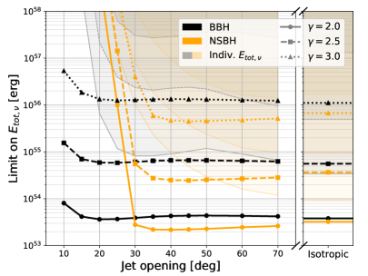
Population studies are performed by stacking (a) all 72 BBH events, and (b) the 7 NSBH candidates. Figure 4 shows the stacked upper limits on the typical total energy emitted in neutrinos (or the ratio $f_{\nu}$) within these two categories, considering jetted emission with the von Mises model (as a function of the jet opening $\omega$) as well as for isotropic emission, and assuming $E^{-\gamma}$ spectra with $\gamma=2.0,\,2.5,\,3.0$.

For individual follow-ups, as $\theta_{\rm jn}$ is not strongly constrained by GW detections, von Mises emission constraints are mainly dominated by geometrical effects: when the jet opening angle is narrow, there is a very small chance that the Earth is aligned with the jet, while a wide opening leads to a larger spread in total energy, which is hence more difficult to constrain. The limits on the total energy as a function of the jet opening are thus expected to show a typical parabola shape corresponding to a trade-off between these two effects, as illustrated by the envelope of individual limits shown in Figure 4. While the individual results for jetted emission are of little interest due to these limitations, the stacking analysis of this scenario yields some benefit as, statistically, some of the sources are expected to point toward Earth for large enough jet opening angles. This can be seen on Figure 4, in particular for the BBH event sample, with the largest statistics, where the neutrino emission can be constrained down to opening angles as small as $\omega\sim 10-$30\text{\,}\mathrm{\SIUnitSymbolDegree}$$.

For the BBH stacking, the stacked limits in the nominal scenario ($\gamma=2$ and isotropic emission) are $E^{\rm iso}_{\rm tot,\nu}<$3.8\text{\times}{10}^{53}\text{\,}\mathrm{erg}$$ and $f_{\nu}<0.14$, while the best limits from individual follow-ups (for GW200202_154313) are respectively $3.2\text{\times}{10}^{54}\text{\,}\mathrm{erg}$ and $2.4$. For the NSBH population, the corresponding limits are $E^{\rm iso}_{\rm tot,\nu}<$3.2\text{\times}{10}^{53}\text{\,}\mathrm{erg}$$ and $f_{\nu}<0.88$, with the best individual limits being (for GW190814) $9.5\text{\times}{10}^{53}\text{\,}\mathrm{erg}$ and $2.2$, respectively.

Finally, it is worth noticing that the statistical power of the BBH stacking already allows the exploration of reasonable values for $f_{\nu}$ (in the context of the assumed simple power-law spectrum), while all individual limits on this parameter are above 1, corresponding to a neutrino emission higher than the GW one.

(a)

(b)

Figure 4: 90% upper limits on the per-source typical total energy emitted in neutrinos (left) and on $f_{\nu}$ (right) as a function of the jet opening angle (for von Mises model) and for the isotropic case (rightmost entry). The black (orange) curves correspond to the BBH (NSBH) stacking of mergers detected during O3. The different markers and line styles correspond to different spectral indices $\gamma$. The filled areas with the corresponding colours (merger category) and line styles (spectral index) indicate the envelope of the best individual upper limits.

Supplemental material with all numerical results for individual follow-ups and from the stacking analysis, for the various jet scenarios and assumed spectral indices, can be provided under request.

5 Discussion and conclusions

The search for neutrino counterparts to GW signals detected during the O3 run with the ANTARES detector yields no significant excess. This null result is used to extract upper limits on the neutrino emission, both in terms of the flux normalisation and of the total energy emitted in neutrinos, $E^{\rm iso}_{\rm tot,\nu}$, in particular for the standard case with an $E^{-2}$ spectrum and isotropic emission.

The ANTARES analysis presented in this article benefits from the different event topologies in the detector, leading to all-flavour limits for neutrino energies above $100\text{\,}\mathrm{GeV}$. The constraints are also interpreted in the context of population studies, for which limits can be put on the typical neutrino emission of different categories of sources (here, BBH and NSBH). As the most recent astrophysical models (e.g., [3, 27, 30]) seem to be out of reach for current detectors, such stacking studies may be one of the most promising approaches to identify joint emitters of neutrinos and GWs. More refined stackings may be studied by considering e.g., sub-populations among BBH mergers, such as the ones having similar source characteristics or environments.

The Bayesian analysis performed here considers flat priors, such that the stacking analysis is performed easily by multiplying the individual posterior distributions. Different priors (e.g., non-informative Jeffreys prior [31]) introduce correlations between the GW follow-ups and would only be possible by performing the posterior marginalisation over all GW events at once, therefore requiring more sophisticated integration techniques than the one employed in this paper.

First constraints on jetted emission for a von Mises model and for different spectral indices are derived as well. In the absence of the determination of any jet direction from the GW data or any electromagnetic observations, these results are only indirectly deducted from the stacking analysis. In future observation campaigns, any such measurement, even for one or a few sources, would allow for deriving direct constraints, as well as considering more complex jet models.

Though the ANTARES detector has been decommissioned in 2022, the KM3NeT experiment [32] has taken over the observation of the neutrino sky from the depths of the Mediterranean Sea. Data from the first few lines of KM3NeT/ORCA has already been used to perform an initial search for neutrino counterparts to the O3 events [33]. With more lines being deployed up to $\sim$ 2026, KM3NeT/ARCA and ORCA are expected to provide complementary coverage of the transient sky with respect to IceCube, increasing the chances to get significant individual detections and creating new opportunities for joint analyses.

The next GW observing period, O4, is expected to start in 2023, including the KAGRA detector in addition to LIGO and Virgo [34]. With an expected number of detections of the order of one hundred per year, population studies will become even more relevant.

Lastly, combinations with ZTF [35] or Vera C. Rubin [36] surveys and Target of Opportunity programs may help pinpoint candidate host galaxies for observed binary mergers, and allow more detailed analyses using the electromagnetic information and the environment characterisation as inputs for the prediction and constraint of the neutrino emission. More generally, there are still only a few models on the processes leading to neutrino production during binary merger events in the literature [3, 4, 5, 27, 30], and further theoretical developments in the coming years may bring new light to past, present, and future observations.

References

- [1] LIGO Scientific, Virgo collaboration, Observation of Gravitational Waves from a Binary Black Hole Merger, Phys. Rev. Lett. 116 (2016) 061102 [1602.03837].
- [2] B.P. Abbott et al., Multi-messenger Observations of a Binary Neutron Star Merger, Astrophys. J. Lett. 848 (2017) L12 [1710.05833].
- [3] S.S. Kimura, K. Murase, I. Bartos, K. Ioka, I.S. Heng and P. Mészáros, Transejecta high-energy neutrino emission from binary neutron star mergers, Phys. Rev. D 98 (2018) 043020 [1805.11613].
- [4] S.S. Kimura, K. Murase, P. Mészáros and K. Kiuchi, High-Energy Neutrino Emission from Short Gamma-Ray Bursts: Prospects for Coincident Detection with Gravitational Waves, Astrophys. J. Lett. 848 (2017) L4 [1708.07075].
- [5] K. Kotera and J. Silk, Ultrahigh Energy Cosmic Rays and Black Hole Mergers, Astrophys. J. Lett. 823 (2016) L29 [1602.06961].
- [6] ANTARES collaboration, Search for neutrino counterparts of gravitational-wave events detected by LIGO and Virgo during run O2 with the ANTARES telescope, Eur. Phys. J. C 80 (2020) 487 [2003.04022].
- [7] Baikal-GVD collaboration, Search for High-Energy Neutrinos from GW170817 with the Baikal-GVD Neutrino Telescope, JETP Lett. 108 (2018) 787 [1810.10966].
- [8] IceCube collaboration, IceCube search for neutrinos coincident with gravitational wave events from LIGO/Virgo run O3, 2208.09532.
- [9] Super-Kamiokande collaboration, Search for neutrinos in coincidence with gravitational wave events from the LIGO-Virgo O3a Observing Run with the Super-Kamiokande detector, Astrophys. J. 918 (2021) 78 [2104.09196].
- [10] LIGO Scientific, Virgo collaboration, GWTC-2: Compact Binary Coalescences Observed by LIGO and Virgo During the First Half of the Third Observing Run, Phys. Rev. X 11 (2021) 021053 [2010.14527].
- [11] LIGO Scientific, VIRGO collaboration, GWTC-2.1: Deep Extended Catalog of Compact Binary Coalescences Observed by LIGO and Virgo During the First Half of the Third Observing Run, 2108.01045.
- [12] LIGO Scientific, VIRGO, KAGRA collaboration, GWTC-3: Compact Binary Coalescences Observed by LIGO and Virgo During the Second Part of the Third Observing Run, 2111.03606.
- [13] LIGO Scientific, VIRGO, KAGRA collaboration, Observation of Gravitational Waves from Two Neutron Star–Black Hole Coalescences, Astrophys. J. Lett. 915 (2021) L5 [2106.15163].
- [14] NASA/GSFC, “Flexible image transport system (fits).” https://fits.gsfc.nasa.gov/, 2021.
- [15] ANTARES collaboration, ANTARES: the first undersea neutrino telescope, Nucl. Instrum. Meth. A 656 (2011) 11 [1104.1607].
- [16] ANTARES collaboration, A fast algorithm for muon track reconstruction and its application to the ANTARES neutrino telescope, Astropart. Phys. 34 (2011) 652 [1105.4116].
- [17] ANTARES collaboration, An algorithm for the reconstruction of neutrino-induced showers in the ANTARES neutrino telescope, Astron. J. 154 (2017) 275 [1708.03649].
- [18] ANTARES collaboration, All-sky search for high-energy neutrinos from gravitational wave event GW170104 with the Antares neutrino telescope, Eur. Phys. J. C 77 (2017) 911 [1710.03020].
- [19] ANTARES, IceCube, Pierre Auger, LIGO Scientific, Virgo collaboration, Search for High-energy Neutrinos from Binary Neutron Star Merger GW170817 with ANTARES, IceCube, and the Pierre Auger Observatory, Astrophys. J. Lett. 850 (2017) L35 [1710.05839].
- [20] B. Baret et al., Bounding the Time Delay between High-energy Neutrinos and Gravitational-wave Transients from Gamma-ray Bursts, Astropart. Phys. 35 (2011) 1 [1101.4669].
- [21] C. Tamburini et al., Deep-sea bioluminescence blooms after dense water formation at the ocean surface, PLOS ONE 8 (2013) 1.
- [22] ANTARES collaboration, Monte Carlo simulations for the ANTARES underwater neutrino telescope, JCAP 01 (2021) 064 [2010.06621].
- [23] ANTARES collaboration, First all-flavor neutrino pointlike source search with the ANTARES neutrino telescope, Phys. Rev. D 96 (2017) 082001 [1706.01857].
- [24] ANTARES collaboration, First search for neutrinos in correlation with gamma-ray bursts with the ANTARES neutrino telescope, JCAP 03 (2013) 006 [1302.6750].
- [25] F. Folger, Search for a diffuse cosmic neutrino flux using shower events in the ANTARES neutrino telescope, Ph.D. thesis, Erlangen - Nuremberg U., 2014.
- [26] M. Bustamante and M. Ahlers, Inferring the flavor of high-energy astrophysical neutrinos at their sources, Phys. Rev. Lett. 122 (2019) 241101 [1901.10087].
- [27] M. Ahlers and L. Halser, Neutrino Fluence from Gamma-Ray Bursts: Off-Axis View of Structured Jets, Mon. Not. Roy. Astron. Soc. 490 (2019) 4935 [1908.06953].
- [28] R. Fisher, Dispersion on a sphere, Proceedings of the Royal Society of London. Series A. Mathematical and Physical Sciences 217 (1953) 295.
- [29] D. Veske, Z. Márka, I. Bartos and S. Márka, Neutrino emission upper limits with maximum likelihood estimators for joint astrophysical neutrino searches with large sky localizations, JCAP 05 (2020) 016 [2001.00566].
- [30] V. Decoene, C. Guépin, K. Fang, K. Kotera and B.D. Metzger, High-energy neutrinos from fallback accretion of binary neutron star merger remnants, JCAP 04 (2020) 045 [1910.06578].
- [31] H. Jeffreys, An invariant form for the prior probability in estimation problems, Proceedings of the Royal Society of London. Series A. Mathematical and Physical Sciences 186 (1946) 453.
- [32] KM3NeT collaboration, Letter of intent for KM3NeT 2.0, J. Phys. G 43 (2016) 084001 [1601.07459].
- [33] KM3NeT collaboration, Search for neutrino counterparts from gravitational waves from the run O3 with KM3NeT, Paper under preparation (2023) .
- [34] KAGRA, LIGO Scientific, Virgo, VIRGO collaboration, Prospects for observing and localizing gravitational-wave transients with Advanced LIGO, Advanced Virgo and KAGRA, Living Rev. Rel. 21 (2018) 3 [1304.0670].
- [35] E.C. Bellm et al., The Zwicky Transient Facility: System Overview, Performance, and First Results, Publications of the Astronomical Society of the Pacific 131 (2018) 018002.
- [36] I. Andreoni et al., Target-of-opportunity Observations of Gravitational-wave Events with Vera C. Rubin Observatory, Astrophys. J. Supp. 260 (2022) 18 [2111.01945].