Best Arm Identification for Stochastic Rising Bandits

Abstract

Stochastic Rising Bandits (SRBs) model sequential decision-making problems in which the expected reward of the available options increases every time they are selected. This setting captures a wide range of scenarios in which the available options are learning entities whose performance improves (in expectation) over time. While previous works addressed the regret minimization problem, this paper focuses on the fixed-budget Best Arm Identification (BAI) problem for SRBs. In this scenario, given a fixed budget of rounds, we are asked to provide a recommendation about the best option at the end of the identification process. We propose two algorithms to tackle the above-mentioned setting, namely R-UCBE, which resorts to a UCB-like approach, and R-SR, which employs a successive reject procedure. Then, we prove that, with a sufficiently large budget, they provide guarantees on the probability of properly identifying the optimal option at the end of the learning process. Furthermore, we derive a lower bound on the error probability, matched by our R-SR (up to logarithmic factors), and illustrate how the need for a sufficiently large budget is unavoidable in the SRB setting. Finally, we numerically validate the proposed algorithms in synthetic and real-world environments and compare them with the currently available BAI strategies.

1 Introduction

Multi-Armed Bandits (MAB, Lattimore and Szepesvári, 2020) are a well-known framework that effectively solves learning problems requiring sequential decisions. Given a time horizon, the learner chooses, at each round, a single option (a.k.a. arm) and observes the corresponding noisy reward, which is a realization of an unknown distribution. The MAB problem is commonly studied in two flavours: regret minimization (Auer et al., 2002) and best arm identification (Bubeck et al., 2009). In regret minimization, the goal is to control the cumulative loss w.r.t. the optimal arm over a time horizon. Conversely, in best arm identification, the goal is to provide a recommendation about the best arm at the end of the time horizon. Specifically, we are interested in the fixed-budget scenario, where we seek to minimize the error probability of recommending the wrong arm at the end of the time budget, no matter the loss incurred during learning.

This work focuses on the Stochastic Rising Bandits (SRB), a specific instance of the rested bandit (Tekin and Liu, 2012) setting in which the expected reward of an arm increases according to the number of times it has been pulled. Online learning in such a scenario has been recently addressed from a regret minimization perspective by Metelli et al. (2022), in which the authors provide no-regret algorithms for the SRB setting in both the rested and restless cases. The SRB setting models several real-world scenarios where arms improve their performance over time. A classic example is the so-called Combined Algorithm Selection and Hyperparameter optimization (CASH, Thornton et al., 2013; Kotthoff et al., 2017; Erickson et al., 2020; Li et al., 2020; Zöller and Huber, 2021), a problem of paramount importance in Automated Machine Learning (AutoML, Feurer et al., 2015; Yao et al., 2018; Hutter et al., 2019; Mussi et al., 2023). In CASH, the goal is to identify the best learning algorithm together with the best hyperparameter configuration for a given ML task (e.g., classification or regression). In this problem, every arm represents a hyperparameter tuner acting on a specific learning algorithm. A pull corresponds to a unit of time/computation in which we improve (on average) the hyperparameter configuration (via the tuner) for the corresponding learning algorithm. CASH was handled in a bandit Best Arm Identification (BAI) fashion in Li et al. (2020) and Cella et al. (2021). The former handles the problem by considering rising rested bandits with deterministic rewards, failing to represent the intrinsic uncertain nature of such processes. Instead, the latter, while allowing stochastic rewards, assumes that the expected rewards evolve according to a known parametric functional class, whose parameters have to be learned.

Original Contributions  In this paper, we address the design of algorithms to solve the BAI task in the rested SRB setting when a fixed budget is provided. More specifically, we are interested in algorithms guaranteeing a sufficiently large probability of recommending the arm with the largest expected reward at the end of the time budget (as if only this arm were pulled from the beginning). The main contributions of the paper are summarized as follows:

• We propose two algorithms to solve the BAI problem in the SRB setting: R-UCBE (an optimistic approach, Section 4) and R-SR (a phases-based rejection algorithm, Section 5). First, we introduce specifically designed estimators required by the algorithms (Section 3). Then, we provide guarantees on the error probability of the misidentification of the best arm.

• We derive the first error probability lower bound for the SRB setting, matched by our R-SR algorithm up to logarithmic factors, which highlights the complexity of the problem and the need for a sufficiently large time budget (Section 6).

• Finally, we conduct numerical simulations on synthetically generated data and a real-world online best model selection problem. We compare the proposed algorithms with the ones available in the bandit literature to tackle the SRB problem (Section 8).

2 Problem Formulation

In this section, we revise the Stochastic Rising Bandits (SRB) setting (Heidari et al., 2016; Metelli et al., 2022). Then, we formulate our best arm identification problem, introduce the definition of error probability, and provide a preliminary characterization of the problem.

Setting  We consider a rested Multi-Armed Bandit problem $\bm{\nu}=(\nu_{i})_{i\in\llbracket K\rrbracket}$ with a finite number of arms $K$. Let $T\in\mathbb{N}$ be the time budget of the learning process. At every round $t\in\llbracket T\rrbracket$, the agent selects an arm $I_{t}\in\llbracket K\rrbracket$, plays it, and observes a reward $x_{t}\sim\nu_{I_{t}}(N_{I_{t},t})$, where $\nu_{I_{t}}(N_{I_{t},t})$ is the reward distribution of the chosen arm $I_{t}$ at round $t$ and depends on the number of pulls performed so far $N_{i,t}\coloneqq\sum_{\tau=1}^{t}\mathds{1}\{I_{\tau}=i\}$ (i.e., rested). The rewards are stochastic, formally $x_{t}\coloneqq\mu_{I_{t}}(N_{I_{t},t})+\eta_{t}$, where $\mu_{I_{t}}(\cdot)$ is the expected reward of arm $I_{t}$ and $\eta_{t}$ is a zero-mean $\sigma^{2}$-subgaussian noise, conditioned to the past. As customary in the bandit literature, we assume that the rewards are bounded in expectation, formally $\mu_{i}(n)\in[0,1],\forall i\in\llbracket K\rrbracket,n\in\llbracket T\rrbracket$. As in (Metelli et al., 2022), we focus on a particular family of rested bandits in which the expected rewards are monotonically non-decreasing and concave in expectation.

Assumption 2.1 (Non-decreasing and concave expected rewards).

Let $\bm{\nu}$ be a rested MAB, defining $\gamma_{i}(n)\coloneqq\mu_{i}(n+1)-\mu_{i}(n)$, for every $n\in\mathbb{N}$ and every arm $i\in\llbracket K\rrbracket$ the rewards are non-decreasing and concave, formally:

$$\text{Non-decreasing:}\quad\gamma_{i}(n)\geq 0,\qquad\qquad\qquad\text{Concave:}\quad\gamma_{i}(n+1)\leq\gamma_{i}(n).$$

Intuitively, the $\gamma_{i}(n)$ represents the increment of the real process $\mu_{i}(\cdot)$ evaluated at the $n$^th pull. Notice that concavity emerges in several settings, such as the best model selection and economics, representing the decreasing marginal returns (Lehmann et al., 2001; Heidari et al., 2016).

Learning Problem  The goal of BAI in the SRB setting is to select the arm providing the largest expected reward with a large enough probability given a fixed budget $T\in\mathbb{N}$. Unlike the stationary BAI problem (Audibert et al., 2010), in which the optimal arm is not changing, in this setting, we need to decide when to evaluate the optimality of an arm. We define optimality by considering the largest expected reward at time $T$. Formally, given a time budget $T$, the optimal arm $i^{*}(T)\in\llbracket K\rrbracket$, which we assume unique, satisfies:

$$i^{*}(T)\coloneqq\operatorname*{arg\,max}_{i\in\llbracket K\rrbracket}\mu_{i}(T),$$

where we highlighted the dependence on $T$ as, with different values of the budget, $i^{*}(T)$ may change. Let $i\in\llbracket K\rrbracket\setminus\{i^{*}(T)\}$ be a suboptimal arm, we define the suboptimality gap as $\Delta_{i}(T)\coloneqq\mu_{i^{*}(T)}(T)-\mu_{i}(T)$. We employ the notation $(i)\in\llbracket K\rrbracket$ to denote the $i$^th best arm at time $T$ (arbitrarily breaking ties), i.e., we have $\Delta_{(2)}(T)\leq\dots\leq\Delta_{(K)}(T)$. Given an algorithm $\mathfrak{A}$ that recommends $\hat{I}^{*}(T)\in\llbracket K\rrbracket$ at the end of the learning process, we measure its performance with the error probability, i.e., the probability of recommending a suboptimal arm at the end of the time budget $T$:

$$e_{T}(\mathfrak{A})\coloneqq{\operatorname*{{\mathbb{P}}}}_{\mathfrak{A}}(\hat{I}^{*}(T)\neq i^{*}(T)).$$

Problem Characterization  We now provide a characterization of a specific class of polynomial functions to upper bound the increments $\gamma_{i}(n)$.

Assumption 2.2 (Bounded $\gamma_{i}(n)$).

Let $\bm{\nu}$ be a rested MAB, there exist $c>0$ and $\beta>1$ such that for every arm $i\in\llbracket K\rrbracket$ and number of pulls $n\in\llbracket 0,T\rrbracket$ it holds that $\gamma_{i}(n)\leq cn^{-\beta}$.

We anticipate that, even if our algorithms will not require such an assumption, it will be used for deriving the lower bound and for providing more human-readable error probability guarantees. Furthermore, we observe that our Assumption 2.2 is fulfilled by a strict superset of the functions employed in Cella et al. (2021).

3 Estimators

In this section, we introduce the estimators of the arm expected reward employed by the proposed algorithms. A visual representation of such estimators is provided in Figure 1.

Let $\varepsilon\in(0,1/2)$ be the fraction of samples collected up to the current time $t$ we use to build estimators of the expected reward. We employ an adaptive arm-dependent window size $h(N_{i,t-1})\coloneqq\lfloor\varepsilon N_{i,t-1}\rfloor$ to include the most recent samples collected only, avoiding the use of samples that are no longer representative. We define the set of the last $h(N_{i,t-1})$ rounds in which the $i$^th arm was pulled as:

$$\mathcal{T}_{i,t}\coloneqq\left\{\tau\in\llbracket T\rrbracket:I_{\tau}=i\;\wedge\right.\left.N_{i,\tau}=N_{i,t-1}-l,\,l\in\llbracket 0,h(N_{i,t-1})-1\rrbracket\right\}.$$

Furthermore, the set of the pairs of rounds $\tau$ and $\tau^{\prime}$ belonging to the sets of the last and second-last $h(N_{i,t-1})$-wide windows of the $i$^th arm is defined as:

$$\mathcal{S}_{i,t}\coloneqq\big{\{} (\tau,\tau^{\prime})\in\llbracket T\rrbracket\times\llbracket T\rrbracket:I_{\tau}=I_{\tau^{\prime}}=i\;\wedge N_{i,\tau}=N_{i,t-1}-l,$$

$$\;\,N_{i,\tau^{\prime}}=N_{i,\tau}-h(N_{i,t-1}),\,l\in\llbracket 0,h(N_{i,t-1})-1\rrbracket\big{\}}.$$

In the following, we design a pessimistic estimator and an optimistic estimator of the expected reward of each arm at the end of the budget time $T$, i.e., $\mu_{i}(T)$.

Pessimistic Estimator  The pessimistic estimator $\hat{\mu}_{i}(N_{i,t-1})$ is a negatively biased estimate of $\mu_{i}(T)$ obtained assuming that the function $\mu_{i}(\cdot)$ remains constant up to time $T$. This corresponds to the minimum admissible value under Assumption 2.1 (due to the Non-decreasing constraint). This estimator is an average of the last $h(N_{i,t-1})$ observed rewards collected from the $i$^th arm, formally:

$$\hat{\mu}_{i}(N_{i,t-1})\coloneqq\frac{1}{h(N_{i,t-1})}\sum_{\tau\in\mathcal{T}_{i,t}}x_{\tau}.$$ (1)

The estimator enjoys the following concentration property.

Lemma 3.1 (Concentration of $\hat{\mu}_{i}$).

Under Assumption 2.1, for every $a>0$, simultaneously for every arm $i\in\llbracket K\rrbracket$ and number of pulls $n\in\llbracket 0,T\rrbracket$, with probability at least $1-2TKe^{-a/2}$ it holds that:

$$\hat{\beta}_{i}(n)-\hat{\zeta}_{i}(n)\leq\hat{\mu}_{i}(n)-\mu_{i}(n)\leq\hat{\beta}_{i}(n),$$

where $\text{ }\hat{\beta}_{i}(n)\coloneqq\sigma\sqrt{\frac{a}{h(n)}}\text{ }$ and $\text{ }\hat{\zeta}_{i}(n)\coloneqq\frac{1}{2}(2T-n+h(n)-1)\,\gamma_{i}(n-h(n)+1)$.

Figure 1: Graphical representation of the pessimistic $\hat{\mu}_{i}(N_{i,t-1})$ and the optimistic $\check{\mu}_{i}^{T}(N_{i,t-1})$ estimators.

As supported by intuition, we observe that the estimator is affected by a negative bias that is represented by $\hat{\zeta}_{i}(n)$ that vanishes as $n\rightarrow\infty$ under Assumption 2.1 with a rate that depends on the increment functions $\gamma_{i}(\cdot)$. Considering also the term $\hat{\beta}_{i}(n)$ and recalling that $h(n)=\mathcal{O}(n)$, under Assumption 2.2, the overall concentration rate is $\mathcal{O}(n^{-1/2}+cTn^{-\beta})$.

Optimistic Estimator  The optimistic estimator $\check{\mu}_{i}^{T}(N_{i,t-1})$ is a positively biased estimation of $\mu_{i}(T)$ obtained assuming that function $\mu_{i}(\cdot)$ linearly increases up to time $T$. This corresponds to the maximum value admissible under Assumption 2.1 (due to the Concavity constraint). The estimator is constructed by adding to the pessimistic estimator $\hat{\mu}_{i}(N_{i,t-1})$ an estimate of the increment occurring in the next step up to $T$. The latter uses the last $2h(N_{i,t-1})$ samples to obtain an upper bound of such growth thanks to the concavity assumption, formally:

$$\check{\mu}_{i}^{T}(N_{i,t-1})\coloneqq\hat{\mu}_{i}(N_{i,t-1})+\sum_{(j,k)\in\mathcal{S}_{i,t}}(T-j)\frac{x_{j}-x_{k}}{h(N_{i,t-1})^{2}}.$$ (2)

The estimator displays the following concentration guarantee.

Lemma 3.2 (Concentration of $\check{\mu}_{i}^{T}$).

Under Assumption 2.1, for every $a>0$, simultaneously for every arm $i\in\llbracket K\rrbracket$ and number of pulls $n\in\llbracket 0,T\rrbracket$, with probability at least $1-2TKe^{-a/10}$ it holds that:

$$\check{\beta}_{i}^{T}(n)\leq\check{\mu}_{i}^{T}(n)-\mu_{i}(n)\leq\check{\beta}_{i}^{T}(n)+\check{\zeta}_{i}^{T}(n),$$

where $\text{ }\check{\beta}_{i}^{T}(n)\coloneqq\sigma\cdot(T-n+h(n)-1)\sqrt{\frac{a}{h(n)^{3}}}\text{}\,$ and $\,\text{}\check{\zeta}_{i}^{T}(n)\coloneqq\frac{1}{2}(2T-n+h(n)-1)\,\gamma_{i}(n-2h(n)\!+\!1)$.

Differently from the pessimistic estimation, the optimistic one displays a positive vanishing bias $\check{\zeta}_{i}^{T}(n)$. Under Assumption 2.2, we observe that the overall concentration rate is $\mathcal{O}(Tn^{-3/2}+cTn^{-\beta})$.

4 Optimistic Algorithm: Rising Upper Confidence Bound Exploration

In this section, we introduce and analyze Rising Upper Confidence Bound Exploration (R-UCBE) an optimistic error probability minimization algorithm for the SRB setting with a fixed budget. The algorithm explores by means of a UCB-like approach and, for this reason, makes use of the optimistic estimator $\check{\mu}_{i}^{T}$ plus a bound to account for the uncertainty of the estimation.

Algorithm  The algorithm, whose pseudo-code is reported in Algorithm 1, requires as input an exploration parameter $a\geq 0$, the window size $\varepsilon\in(0,1/2)$, the time budget $T$, and the number of arms $K$. At first, it initializes to zero the counters $N_{i,0}$, and sets to $+\infty$ the upper bounds $B_{i}^{T}(N_{i,0})$ of all the arms (Line 1). Subsequently, at each time $t\in\llbracket T\rrbracket$, the algorithm selects the arm $I_{t}$ with the largest upper confidence bound (Line 1):

$$I_{t}\in\operatorname*{arg\,max}_{i\in\llbracket K\rrbracket}B_{i}^{T}(N_{i,t-1})\coloneqq\check{\mu}_{i}^{T}(N_{i,t-1})+\check{\beta}_{i}^{T}(N_{i,t-1}),$$ (3)

$$\text{with:}\quad\check{\beta}_{i}^{T}(N_{i,t-1})\coloneqq\sigma\cdot(T-N_{i,t-1}+h(N_{i,t-1})-1)\sqrt{\frac{a}{h(N_{i,t-1})^{3}}},$$ (4)

where $\check{\beta}_{i}^{T}(N_{i,t-1})$ represents the exploration bonus (a graphical representation is reported in Figure 1). Once the arm is chosen, the algorithm plays it and observes the feedback $x_{t}$ (Line 1). Then, the optimistic estimate $\check{\mu}_{I_{t}}^{T}(N_{I_{t},t})$ and the exploration bonus $\check{\beta}_{I_{t}}^{T}(N_{I_{t},t})$ of the selected arm $I_{t}$ are updated (Lines 1-1). The procedure is repeated until the algorithm reaches the time budget $T$. The final recommendation of the best arm is performed using the last computed values of the bounds $B_{i}^{T}(N_{i,T})$, returning the arm $\hat{I}^{*}(T)$ corresponding to the largest upper confidence bound (Line 1).

Bound on the Error Probability of R-UCBE  We now provide bounds on the error probability for R-UCBE. We start with a general analysis that makes no assumption on the increments $\gamma_{i}(\cdot)$ and, then, we provide a more explicit result under Assumption 2.2. The general result is formalized as follows.

Theorem 4.1.

Under Assumption 2.1, let $a^{*}$ be the largest positive value of $a$ satisfying:

$$T-\sum_{i\neq i^{*}(T)}y_{i}(a)\geq 1,$$ (5)

where for every $i\in\llbracket K\rrbracket$, $y_{i}(a)$ is the largest integer for which it holds:

$$\underbrace{T\gamma_{i}(\lfloor(1-2\varepsilon)y\rfloor)}_{({A})}+\underbrace{2T\sigma\sqrt{\frac{a}{\lfloor\varepsilon y\rfloor^{3}}}}_{({B})}\geq\Delta_{i}(T).$$ (6)

If $a^{*}$ exists, then for every $a\in\left[0,a^{*}\right]$ the error probability of R-UCBE is bounded by:

$$e_{T}(\text{{R-UCBE}\@})\leq 2TK\exp{\left(-\frac{a}{10}\right)}.$$ (7)

Some comments are in order. First, $a^{*}$ is defined implicitly, depending on the constants $\sigma$, $T$, the increments $\gamma_{i}(\cdot)$, and the suboptimality gaps $\Delta_{i}(T)$. In principle, there might exist no $a^{*}>0$ fulfilling condition in Equation (5) (this can happen, for instance, when the budget $T$ is not large enough), and, in such a case, we are unable to provide theoretical guarantees on the error probability of R-UCBE. Second, the result presented in Theorem 4.1 holds for generic increasing and concave expected reward functions. This result shows that, as expected, the error probability decreases when the exploration parameter $a$ increases. However, this behavior stops when we reach the threshold $a^{*}$. Intuitively, the value of $a^{*}$ sets the maximum amount of exploration we should use for learning.

Under Assumption 2.2, i.e., using the knowledge on the increment $\gamma_{i}(\cdot)$ upper bound, we derive a result providing conditions on the time budget $T$ under which $a^{*}$ exists and an explicit value for $a^{*}$.

Corollary 4.2.

Under Assumptions 2.1 and 2.2, if the time budget $T$ satisfies:

$$T\geq\begin{cases}\left(c^{\frac{1}{\beta}}(1-2\varepsilon)^{-1}\;(H_{1,{1}/{\beta}}(T))+(K-1)\right)^{\frac{\beta}{\beta-1}}&\text{if }\beta\in(1,3/2)\\ \left(c^{\frac{2}{3}}(1-2\varepsilon)^{-\frac{2}{3}\beta}\;(H_{1,{2}/{3}}(T))+(K-1)\right)^{3}&\text{if }\beta\in[3/2,+\infty)\end{cases},$$ (8)

there exists $a^{*}>0$ defined as:

$$a^{*}=\begin{cases}\frac{\epsilon^{3}}{4\sigma^{2}}\left(\left(\frac{T^{1-1/\beta}-(K-1)}{H_{1,1/\beta}(T)}\right)^{\beta}-c(1-2\varepsilon)^{-\beta}\right)^{2}&\text{if}\;\beta\in\left(1,3/2\right)\\ \frac{\epsilon^{3}}{4\sigma^{2}}\left(\left(\frac{T^{1/3}-(K-1)}{H_{1,2/3}(T)}\right)^{3/2}-c(1-2\varepsilon)^{-\beta}\right)^{2}&\text{if}\;\beta\in\left[3/2,+\infty\right)\end{cases},$$

where $H_{1,\eta}(T)\coloneqq\sum_{i\neq i^{*}(T)}{}\frac{1}{\Delta_{i}^{\eta}(T)}$ for $\eta>0$. Then, for every $a\in\left[0,a^{*}\right]$, the error probability of R-UCBE is bounded by:

$$e_{T}(\text{{R-UCBE}\@})\leq 2TK\exp{\left(-\frac{a}{10}\right)}.$$

First of all, we notice that the error probability $e_{T}(\text{{R-UCBE}\@})$ presented in Theorem 4.2 holds under the condition that the time budget $T$ fulfills Equation (8). We defer a more detailed discussion on this condition to Remark 5.1, where we show that the existence of a finite value of $T$ fulfilling Equation (8) is ensured under mild conditions.

Let us remark that term $H_{1,\eta}(T)$ characterizes the complexity of the SRB setting, corresponding to term $H_{1}$ of Audibert et al. (2010) for the classical BAI problem when $\eta=2$. As expected, in the small-$\beta$ regime (i.e., $\beta\in(1,3/2]$), looking at the dependence of $H_{1,1/\beta}(T)$ on $\beta$, we realize that the complexity of a problem decreases as the parameter $\beta$ increases. Indeed, the larger $\beta$, the faster the expected reward reaches a stationary behavior. Nevertheless, even in the large-$\beta$ regime (i.e., $\beta>3/2$), the complexity of the problem is governed by $H_{1,2/3}(T)$, leading to an error probability larger than the corresponding one for BAI in standard bandits (Audibert et al., 2010). This can be explained by the fact that R-UCBE uses the optimistic estimator that, as shown in Section 3, enjoys a slower concentration rate compared to the standard sample mean, even for stationary bandits.

Input : Time budget $T$, Number of arms $K$,

Window size $\varepsilon$, Exploration parameter $a$

1

2Initialize $\text{ }N_{i,0}=0$,

3 Initialize $\text{ }B_{i}^{T}(0)=+\infty,\forall i\in\llbracket K\rrbracket$

4

5for $t\in\llbracket T\rrbracket$ do

6       Compute $I_{t}\in\operatorname*{arg\,max}_{i\in\llbracket K\rrbracket}B_{i}^{T}(N_{i,t-1})$

7       Pull arm $I_{t}$ and observe $x_{t}$

8       $N_{I_{t},t}\leftarrow N_{I_{t},t-1}+1$

9       $N_{i,t}\leftarrow N_{i,t-1},\quad\forall i\neq I_{t}$

10       Update $\check{\mu}_{I_{t}}^{T}(N_{I_{t},t})$

11       Update $\check{\beta}_{I_{t}}^{T}(N_{I_{t},t})$

12       Compute $B_{I_{t}}^{T}(N_{I_{t},t})=\check{\mu}_{I_{t}}^{T}(N_{I_{t},t})+\check{\beta}_{I_{t}}^{T}(N_{I_{t},t})$

13 end for

14Recommend $\widehat{I}^{*}(T)\in\operatorname*{arg\,max}_{i\in\llbracket K\rrbracket}B_{i}^{T}(N_{i,T})$

Algorithm 1 R-UCBE.

1

Input : Time budget $T$, Number of arms $K$,

Window size $\varepsilon$

2

3Initialize $\text{ }t\leftarrow 1,\;N_{0}=0,\;\mathcal{X}_{0}=\llbracket K\rrbracket$

4

5for $j\in\llbracket K-1\rrbracket$ do

6       for $i\in\mathcal{X}_{j-1}$ do

7             for $l\in\llbracket N_{j-1}+1,N_{j}\rrbracket$ do

8                   Pull arm $i$ and observe $x_{t}$

9                   $t\leftarrow t+1$

10             end for

11            Update $\hat{\mu}_{i}(N_{j})$

12       end for

13      Define $\overline{I}_{j}\in\operatorname*{arg\,min}_{i\in\mathcal{X}_{j-1}}\hat{\mu}_{i}(N_{j})$

14       Update $\mathcal{X}_{j}=\mathcal{X}_{j-1}\,\setminus\{\overline{I}_{j}\}$

15 end for

16Recommend $\widehat{I}^{*}(T)\in\mathcal{X}_{K-1}$ (unique)

Algorithm 2 R-SR.

This two-regime behavior has an interesting interpretation when comparing Corollary 4.2 with Theorem 4.1. Indeed, $\beta=3/2$ is the break-even threshold in which the two terms of the l.h.s. of Equation (6) have the same convergence rate. Specifically, the term $({A})$ takes into account the expected rewards growth (i.e., the bias in the estimators), while $({B})$ considers the uncertainty in the estimations of the R-UCBE algorithm (i.e., the variance). Intuitively, when the expected reward function displays a slow growth (i.e., $\gamma_{i}(n)\leq cn^{-\beta}$ with $\beta<3/2$), the bias term $({A})$ dominates the variance term $({B})$ and the value of $a^{*}$ changes accordingly. Conversely, when the variance term $({B})$ is the dominant one (i.e., $\gamma_{i}(n)\leq cn^{-\beta}$ with $\beta>3/2$), the threshold $a^{*}$ is governed by the estimation uncertainty, being the bias negligible.

As common in optimistic algorithms for BAI (Audibert et al., 2010), setting a theoretically sound value of exploration parameter $a$ (i.e., computing $a^{*}$), requires additional knowledge of the setting, namely the complexity index $H_{1,\eta}(T)$. In the next section, we propose an algorithm that relaxes this requirement.

5 Phase-Based Algorithm: Rising Successive Rejects

In this section, we introduce the Rising Successive Rejects (R-SR), a phase-based solution inspired by the one proposed by Audibert et al. (2010), which overcomes the drawback of R-UCBE of requiring knowledge of $H_{1,\eta}(T)$.

Algorithm  R-SR, whose pseudo-code is reported in Algorithm 2, takes as input the time budget $T$ and the number of arms $K$. At first, it initializes the set of the active arms $\mathcal{X}_{0}$ with all the available arms (Line 2). This set will contain the arms that are still eligible candidates to be recommended. The entire process proceeds through $K-1$ phases. More specifically, during the $j$^th phase, the arms still remaining in the active arms set $\mathcal{X}_{j-1}$ are played (Line 2) for $N_{j}-N_{j-1}$ times each, where:

$$N_{j}\coloneqq\left\lceil\frac{1}{\overline{\log}(K)}\frac{T-K}{K+1-j}\right\rceil,$$ (9)

and $\overline{\log}(K)\coloneqq\frac{1}{2}+\sum_{i=2}^{K}\frac{1}{i}$. At the end of each phase, the arm with the smallest value of the pessimistic estimator $\hat{\mu}_{i}(N_{j})$ is discarded from the set of active arms (Line 2). At the end of the $(K-1)$^th phase, the algorithm recommends the (unique) arm left in $\mathcal{X}_{K-1}$ (Line 2).

It is worth noting that R-SR makes use of the pessimistic estimator $\hat{\mu}_{i}(n)$. Even if both estimators defined in Section 3 are viable for R-SR, the choice of using the pessimistic estimator is justified by its better concentration rate $\mathcal{O}(n^{-1/2})$ compared to that of the optimistic estimator $\mathcal{O}(Tn^{-3/2})$, being $n\leq T$ (see Section 3).

Note that the phase lengths are the ones adopted by Audibert et al. (2010). This choice allows us to provide theoretical results without requiring domain knowledge (still under a large enough budget). An optimized version of $N_{j}$ may be derived assuming full knowledge of the gaps $\Delta_{i}(T)$, but, unfortunately, such a hypothetical approach would have similar drawbacks as R-UCBE.

Bound on the Error Probability of R-SR  The following theorem provides the guarantee on the error probability for the R-SR algorithm.

Theorem 5.1.

Under Assumptions 2.1 and 2.2, if the time budget $T$ satisfies:

$$T\geq 2^{\frac{{\beta+1}}{\beta-1}}c^{\frac{1}{\beta-1}}\mkern 1.5mu\overline{\mkern-1.5mu\log\mkern-1.5mu}\mkern 1.5mu(K)^{\frac{\beta}{\beta-1}}\max_{i\in\llbracket 2,K\rrbracket}\left\{i^{\frac{\beta}{\beta-1}}\Delta_{(i)}(T)^{-{\frac{1}{\beta-1}}}\right\},$$ (10)

then, the error probability of R-SR is bounded by:

$$e_{T}(\text{{R-SR}\@})\leq\frac{K(K-1)}{2}\ \exp\left(-\frac{\varepsilon}{8\sigma^{2}}\cdot\frac{T-K}{\mkern 1.5mu\overline{\mkern-1.5mu\log\mkern-1.5mu}\mkern 1.5mu(K)H_{2}(T)}\right),$$

where $H_{2}(T)\coloneqq\max_{i\in\llbracket K\rrbracket}\left\{i\Delta_{(i)}(T)^{-2}\right\}\text{ }$ and $\text{ }\mkern 1.5mu\overline{\mkern-1.5mu\log\mkern-1.5mu}\mkern 1.5mu(K)=\frac{1}{2}+\sum_{i=2}^{K}{\frac{1}{i}}$.

Similar to the R-UCBE, the complexity of the problem is characterized by term $H_{2}(T)$ that, for the standard MAB setting, reduces to the $H_{2}$ term of Audibert et al. (2010). Furthermore, when the condition of Equation (10) on the time budget $T$ is satisfied, the error probability coincides with that of the SR algorithm for standard MABs (apart for constant terms). The following remark elaborates on the conditions of Equations (8) and (10) about the minimum requested time budget.

Remark 5.1 (About the minimum time budget $T$).

To satisfy the $e_{T}$ bounds presented in Corollary 4.2 and Theorem 5.1, R-UCBE and R-SR require the conditions provided by Equations (8) and (10) about the time budget $T$, respectively. First, let us notice that if the suboptimal arms converge to an expected reward different from that of the optimal arm as $T\rightarrow+\infty$, it is always possible to find a finite value of $T<+\infty$ such that these conditions are fulfilled. Formally, assume that there exists $T_{0}<+\infty$ and that for every $T\geq T_{0}$ we have that for all suboptimal arms $i\neq i^{*}(T)$ it holds that $\Delta_{i}(T)\geq\Delta_{\infty}>0$. In such a case, the l.h.s. of Equations (8) and (10) are upper bounded by a function of $\Delta_{\infty}$ and are independent on $T$. Instead, if a suboptimal arm converges to the same expected reward as the optimal arm when $T\rightarrow+\infty$, the identification problem is more challenging and, depending on the speed at which the two arms converge as a function of $T$, might slow down the learning process arbitrarily. This should not surprise as the BAI problem becomes non-learnable even in standard (stationary) MABs when multiple optimal arms are present (Heide et al., 2021).

6 Lower Bound

In this section, we investigate the complexity of the BAI problem for SRBs with a fixed budget.

Minimum time budget $\mathbf{T}$  We show that, under Assumptions 2.1 and 2.2, any algorithm requires a minimum time budget $T$ to be guaranteed to identify the optimal arm, even in a deterministic setting.

Theorem 6.1.

For every algorithm $\mathfrak{A}$, there exists a deterministic SRB satisfying Assumptions 2.1 and 2.2 such that the optimal arm $i^{*}(T)$ cannot be identified for some time budgets $T$ unless:

$$T\geq H_{1,1/(\beta-1)}(T)=\sum_{i\neq i^{*}(T)}\frac{1}{\Delta_{i}(T)^{\frac{1}{\beta-1}}}.$$ (11)

Theorem 6.1 formalizes the intuition that any of the suboptimal arms must be pulled a sufficient number of times to ensure that, if pulled further, it cannot become the optimal arm. It is worth comparing this bound on the time budget with the corresponding conditions on the minimum time budget requested by Equations (8) and (10) for R-UCBE and R-SR, respectively. Regarding R-UCBE, we notice that the minimum admissible time budget in the small-$\beta$ regime is of order $H_{1,1/\beta}(T)^{\beta/(\beta-1)}$ which is larger than term $H_{1,1/(\beta-1)}(T)$ of Equation (11). Similarly, in the large-$\beta$ regime (i.e., $\beta>3/2$), the R-UCBE requirement is of order $H_{1,2/3}(T)^{3}\geq H_{1,2}(T)$ which is larger than the term of Theorem 6.1 since $1/(\beta-1)<2$. Concerning R-SR, it is easy to show that $H_{1,1/(\beta-1)}(T)\approx\max_{i\in\llbracket 2,K\rrbracket}i\Delta_{(i)}(T)^{-1/(\beta-1)}$, apart from logarithmic terms, by means of the argument provided by (Audibert et al., 2010, Section 6.1). Thus, up to logarithmic terms, Equation (10) provides a tight condition on the minimum budget.

Error Probability Lower Bound  We now present a lower bound on the error probability.

Theorem 6.2.

For every algorithm $\mathfrak{A}$ run with a time budget $T$ fulfilling Equation (11), there exists a SRB satisfying Assumptions 2.1 and 2.2 such that the error probability is lower bounded by:

$$e_{T}(\mathfrak{A})\geq\frac{1}{4}\exp\left(-\frac{8T}{\sigma^{2}H_{1,2}(T)}\right),\ \ \ \text{where}\ \ \ H_{1,2}(T)\coloneqq\sum_{i\neq i^{*}(T)}{}\frac{1}{\Delta_{i}^{2}(T)}.$$

Some comments are in order. First, we stated the lower bound for the case in which the minimum time budget satisfies the inequality of Theorem 6.1, which is a necessary condition for identifying the optimal arm. Second, the lower bound on the error probability matches, up to logarithmic factors, that of our R-SR, suggesting the superiority of this algorithm compared to R-UCBE. Finally, provided that the identifiability condition of Equation (11), such a result corresponds to that of the standard (stationary) MABs (Audibert et al., 2010; Kaufmann et al., 2016). A summary of all the bounds provided in the paper is presented in Table 1.

	Error Probability $e_{T}(\cdot)$	Time Budget $T$
SRB	$\displaystyle\frac{1}{4}\exp\left(-\frac{8T}{\sigma^{2}\sum_{i\neq i^{*}(T)}{}\frac{1}{\Delta_{i}^{2}(T)}}\right)$	$\displaystyle\sum_{i\neq i^{*}(T)}\frac{1}{\Delta_{i}(T)^{\frac{1}{\beta-1}}}$
R-UCBE	$\displaystyle 2\;T\;K\;\exp{\left(-\frac{a}{10}\right)}$	$\begin{cases}\displaystyle\bigg{(}c^{\frac{1}{\beta}}(1-2\varepsilon)^{-1}\;\bigg{(}\sum_{i\neq i^{*}(T)}{}\frac{1}{\Delta_{i}^{1/\beta}(T)}\bigg{)}+(K-1)\bigg{)}^{\frac{\beta}{\beta-1}}\>\,&\text{ if }\beta\in\left(1,3/2\right)\\ \displaystyle\bigg{(}c^{\frac{2}{3}}(1-2\varepsilon)^{-\frac{2}{3}\beta}\;\bigg{(}\sum_{i\neq i^{*}(T)}{}\frac{1}{\Delta_{i}^{2/3}(T)}\bigg{)}+(K-1)\bigg{)}^{3}\ \ \,&\text{ if }\beta\in\left[3/2,+\infty\right)\end{cases}$
R-SR	$\displaystyle\frac{K(K-1)}{2}\ \exp\left(-\frac{\varepsilon}{8\sigma^{2}}\frac{T-K}{\mkern 1.5mu\overline{\mkern-1.5mu\log\mkern-1.5mu}\mkern 1.5mu(K)\displaystyle\max_{i\in\llbracket K\rrbracket}\left\{i\Delta_{(i)}^{-2}(T)\right\}}\right)$	$\displaystyle 2^{\frac{{1+\beta}}{\beta-1}}c^{\frac{1}{\beta-1}}\mkern 1.5mu\overline{\mkern-1.5mu\log\mkern-1.5mu}\mkern 1.5mu(K)^{\frac{\beta}{\beta-1}}\max_{i\in\llbracket 2,K\rrbracket}\left\{i^{\frac{\beta}{\beta-1}}\Delta_{(i)}(T)^{-{\frac{1}{\beta-1}}}\right\}$

Table 1: Bounds on the time budget and error probability: lower for the setting and upper for the algorithms.

7 Related Works

In this section, we summarize the relevant literature related both to the works focusing on the best arm identification problem and rested bandits. The SRB setting was proposed by Heidari et al. (2016) for the first time. Their work and subsequently the one by Metelli et al. (2022) analyzed the problem from a regret minimization point of view.

Best Arm Identification in Stochastic Rising Bandits  As highlighted in Section 1, the works mostly related to ours are the ones by Li et al. (2020) and Cella et al. (2021). They both focus on the BAI problem in the rested setting, given a fixed-budget. More specifically, Li et al. (2020) consider rising rested bandits in which the reward function of each arm increases as it is pulled. However, they limit to deterministic arms and, thus, fail to deal with the intrinsic stochasticity of the real-world processes they want to model. Instead, Cella et al. (2021) deal with the problem of identifying the arm with the smallest loss in a setting where the losses incurred by selecting an arm decrease over time. It is easy to show that such a setting can be transformed straightforwardly in the SRB one. However, the authors develop two algorithms whose theoretical guarantees hold under the assumption that the expected loss follows a specific known parametric functional form, whose parameters are to be estimated. This constitutes a major limitation to the presented work since checking such an assumption is not feasible in real-world settings.

Best Arm Identification  The pure exploration and BAI problems have been first introduced by Bubeck et al. (2009), while algorithms able to learn in such a setting have been provided by Audibert et al. (2010). The work by Gabillon et al. (2012) proposes a unified approach to deal with stochastic best arm identification problems by having either a fixed budget or fixed confidence. However, the stochastic algorithms developed in this line of research only provide theoretical guarantees in settings where the expected reward is stationary over the pulls. Abbasi-Yadkori et al. (2018) propose a method able to handle both the stochastic and adversarial cases, but they do not make explicit use of the properties (e.g., increasing nature) of the expected reward. Finally, (Garivier and Kaufmann, 2016; Kaufmann et al., 2016; Carpentier and Locatelli, 2016) analyze the problem of BAI from the lower bound perspective.

Rested Bandits  Bandit settings in which the evolution of an arm reward depends on the number of times the arm has been pulled, such as the one analyzed in our paper, are generally referred to as rested. A first general formulation of the rested bandit setting appeared in the work by Tekin and Liu (2012) and was further discussed by Mintz et al. (2020) and Seznec et al. (2020). In these works, the evolution of the expected reward of each arm is regulated by a Markovian process that is assumed to visit the same state multiple times. This is not the case for the rising bandits, where the arm expected rewards continuously increase over the time budget. Finally, a specific instance of the rested bandits is constituted by the rotting bandits (Levine et al., 2017; Seznec et al., 2019, 2020), in which the expected payoff for a given arm decreases with the number of pulls. However, as pointed out by Metelli et al. (2022), techniques developed for this setting cannot be directly translated into ours, due to the inherently different nature of the problem.

8 Numerical Validation

In this section, we provide a numerical validation of R-UCBE and R-SR. We compare them with state-of-the-art bandit baselines designed for stationary and non-stationary BAI in a synthetic setting, and we evaluate the sensitivity of R-UCBE to its exploration parameter $a$. Additional details about the experiments presented in this section are available in Appendix E. Additional experimental results on both synthetic settings and in a real-world experiment are available in Appendix F.

Baselines  We compare our algorithms against a wide range of solutions for BAI:

• RR: uniformly pulls all the arms until the budget ends in a round-robin fashion and, in the end, makes a recommendation based on the empirical mean of their reward over the collected samples;

• RR-SW: makes use of the same exploration strategy as RR to pull arms but makes a recommendation based on the empirical mean over the last $\frac{\varepsilon T}{K}$ collected samples from an arm.

• UCB-E and SR (Audibert et al., 2010): algorithms for the stationary BAI problem;

• Prob-1 (Abbasi-Yadkori et al., 2018): an algorithm dealing with the adversarial BAI setting;

• ETC and Rest-Sure (Cella et al., 2021): algorithms developed for the decreasing loss BAI setting.

The hyperparameters required by the above methods have been set as prescribed in the original papers. For both our algorithms and RR-SW, we set $\varepsilon=0.25$.

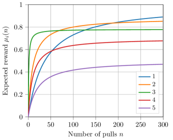
Figure 2: Expected values $\mu_{i}(n)$ for the arms of the synthetic setting.

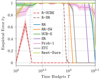
Figure 3: Empirical error rate for the synthetically generated setting (100 runs, mean $\pm$ 95% c.i.).

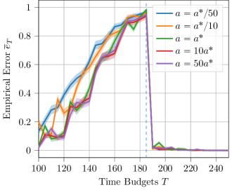
Figure 4: Empirical error rate for the R-UCBE at different $a$ (1000 runs, mean $\pm$ 95% c.i.).

Setting  To assess the quality of the recommendation $\hat{I}^{*}(T)$ provided by our algorithms, we consider a synthetic SRB setting with $K=5$ and $\sigma=0.01$. Figure 2 shows the evolution of the expected values of the arms w.r.t. the number of pulls. In this setting, the optimal arm changes depending on whether $T\in[1,185]$ or $T\in(185,+\infty)$. Thus, when the time budget is close to that value, the problem is more challenging since the optimal and second-best arms expected rewards are close to each other. For this reason, the BAI algorithms are less likely to provide a correct recommendation than for time budgets for which the two expected rewards are well separated. We compare the analyzed algorithms $\mathfrak{A}$ in terms of empirical error $\overline{e}_{T}(\mathfrak{A})$ (the smaller, the better), i.e., the empirical counterpart of $e_{T}(\mathfrak{A})$ averaged over $100$ runs, considering time budgets $T\in[100,3200]$.

Results  The empirical error probability provided by the analyzed algorithms in the synthetically generated setting is presented in Figure 3. We report with a dashed vertical blue line at $T=185$, i.e., the budgets after which the optimal arm no longer changes. Before such a budget, all the algorithms provide large errors (i.e., $\bar{e}_{T}(\mathfrak{A})>0.2$). However, R-UCBE outperforms the others by a large margin, suggesting that an optimistic estimator might be advantageous when the time budget is small. Shortly after $T=185$, R-UCBE starts providing the correct suggestion consistently. R-SR begins to identify the optimal arm (i.e., with $\bar{e}_{T}(\text{{R-SR}\@})<0.05$) for time budgets $T>1000$. Nonetheless, both algorithms perform significantly better than the baseline algorithms used for comparison.

Sensitivity Analysis for the Exploration Parameter of R-UCBE  We perform a sensitivity analysis on the exploration parameter $a$ of R-UCBE. Such a parameter should be set to a value less or equal to $a^{*}$, and the computation of the latter is challenging. We tested the sensitivity of R-UCBE to this hyperparameter by looking at the error probability for $a\in\{a^{*}/50,a^{*}/10,a^{*},10a^{*},50a^{*}\}$. Figure 4 shows the empirical errors of R-UCBE with different parameters $a$, where the blue dashed vertical line denotes the last time the optimal arm changes over the time budget. It is worth noting how, even in this case, we have two significantly different behaviors before and after such a time. Indeed, if $T\leq 185$, we have that a misspecification with larger values than $a^{*}$ does not significantly impact the performance of R-UCBE, while smaller values slightly decrease the performance. Conversely, for $T>185$ learning with different values of $a$ seems not to impact the algorithm performance significantly. This corroborates the previous results about the competitive performance of R-UCBE.

9 Discussion and Conclusions

This paper introduces the BAI problem with a fixed budget for the Stochastic Rising Bandits setting. Notably, such setting models many real-world scenarios in which the reward of the available options increases over time, and the interest is on the recommendation of the one having the largest expected rewards after the time budget has elapsed. In this setting, we presented two algorithms, namely R-UCBE and R-SR providing theoretical guarantees on the error probability. R-UCBE is an optimistic algorithm requiring an exploration parameter whose optimal value requires prior information on the setting. Conversely, R-SR is a phase-based solution that only requires the time budget to run. We established lower bounds for the error probability an algorithm suffers in such a setting, which is matched by our R-SR, up to logarithmic factors. Furthermore, we showed how a requirement on the minimum time budget is unavoidable to ensure the identifiability of the optimal arm. Finally, we validate the performance of the two algorithms in both synthetically generated and real-world settings. A possible future line of research is to derive an algorithm balancing the tradeoff between theoretical guarantees on the $e_{T}$ and the chance of providing such guarantees with lower time budgets.

Appendix A Additional Motivating Examples

In this appendix, we provide two additional motivating examples to better understand and appreciate the SRB setting.

Selection of Athletes for Competitions  Consider the role of a professional trainer for a team, having several athletes (i.e., our arms) to train in order to increase their performances. The final goal is to select a single athlete to represent the team in a competition. The performances of athletes increase when the trainer properly follows them. However, a trainer can follow just one athlete at a time. The trainer can be modeled as an agent performing best-arm (athlete) identification, and the athletes represent the arms that increase their payoffs (i.e., performance) when pulled (i.e., when the trainer follows them).

Online Best Model Selection  Suppose we have to choose among a set of algorithms to maximize a given index (e.g., accuracy) over a training set. In this setting, we expect that all the algorithms progressively increase (on average) the index value and converge to their optimum value with different convergence rates. Therefore, we want to identify which candidate algorithm is the most likely to reach optimal performances, given the budget, and assign the available resources (e.g., computational power or samples). In summary, this problem reduces to the identification, with the largest probability, of the algorithm that converges faster to the optimum. A real-world example of such a scenario is provided in Figure 8.

Appendix B Estimators Efficient Update

In this appendix, we describe how to implement an efficient version (i.e., fully online) of the estimators we presented in the main paper. We resort to the update developed by Metelli et al. [2022]. This update provides a way to achieve an $\mathcal{O}(1)$ computational complexity at each step for the update of the estimates for the pessimistic estimator $\hat{\mu}_{i}(t)$ and optimistic estimator $\check{\mu}_{i}^{T}(t)$.

With a slight abuse of notation, only in this appendix, for the sake of simplicity, we denote with $\overline{x}_{i,n}$ the reward collected at the $n$^th pull from the arm $i$ and with $h_{i,t}=h(N_{i,t-1})$ the window size. Differently, from what we use in the paper, here the reward subscript indicates the arm $i$ and the number of pulls of that arm $n$ instead of the total number of pulls $t$ we used in the definition of $x_{t}$.

More specifically, the pessimistic estimator $\hat{\mu}_{i}$ can be written as:

$$\hat{\mu}_{i}(t)=\frac{\overline{a}_{i}}{h_{i,t}},$$

where the quantity $\overline{a}_{i}$ is updated as follows:

$$\overline{a}_{i}\leftarrow\begin{cases}\overline{a}_{i}+\overline{x}_{i,N_{i,t}}-\overline{x}_{i,N_{i,t}-h_{i,t}}&\ \text{if}\ h_{i,t}=h_{i,t-1}\\ \overline{a}_{i}+\overline{x}_{i,N_{i,t}}&\ \text{otherwise}\end{cases},$$

and $\overline{a}_{i}=0$ as the algorithm starts.

Instead, the optimistic estimator $\check{\mu}_{i}^{T}(t)$, is updated using:

$$\check{\mu}_{i}^{T}(t)=\frac{1}{h_{i,t}}\left(\overline{a}_{i}+\frac{T(\overline{a}_{i}-\overline{b}_{i})}{h_{i,t}}-\frac{\overline{c}_{i}-\overline{d}_{i}}{h_{i,t}}\right).$$

Where the quantity $\overline{a}_{i}$ is defined and updated above and $\overline{b}_{i}$, $\overline{c}_{i}$, and $\overline{d}_{i}$ are updated as follows:

$$\overline{b}_{i} \leftarrow\begin{cases}\overline{b}_{i}+\overline{x}_{i,N_{i,t}-h_{i,t}}-\overline{x}_{i,N_{i,t}-2h_{i,t}}&\ \qquad\qquad\qquad\qquad\ \text{if}\ h_{i,t}=h_{i,t-1}\\ \overline{b}_{i}+\overline{x}_{i,N_{i,t}-2h_{i,t}+1}&\ \qquad\qquad\qquad\qquad\ \text{otherwise}\end{cases},$$

$$\overline{c}_{i} \leftarrow\begin{cases}\overline{c}_{i}+N_{i,t}\cdot\overline{x}_{i,N_{i,t}}-(N_{i,t}-h_{i,t})\cdot\overline{x}_{i,N_{i,t}-h_{i,t}}&\qquad\;\;\text{if}\ h_{i,t}=h_{i,t-1}\\ \overline{c}_{i}+N_{i,t}\cdot\overline{x}_{i,N_{i,t}}&\qquad\;\;\text{otherwise}\end{cases},$$

$$\overline{d}_{i} \leftarrow\begin{cases}\overline{d}_{i}+N_{i,t}\cdot\overline{x}_{i,N_{i,t}-h_{i,t}}-(N_{i,t}-h_{i,t})\cdot\overline{x}_{i,N_{i,t}-2h_{i,t}}&\ \text{if}\ h_{i,t}=h_{i,t-1}\\ \overline{d}_{i}+(N_{i,t}-h_{i,t})\cdot\overline{x}_{i,N_{i,t}-2h_{i,t}+1}+\overline{b}_{i}&\ \text{otherwise}\end{cases}.$$

Similarly to what is presented above, the quantities are initialized to $0$ as the algorithms start.

Appendix C Proofs and Derivations

In this appendix, we provide all the proofs omitted in the main paper. For the sake of generality, we will provide the derivations for a generic choice of the window size of the estimators $h_{i,t}$ which depends on the arm $i\in\llbracket K\rrbracket$ and on the round $t\in\llbracket T\rrbracket$. When needed, we will particularize the choice for the case in which the window size depends on the number of pulls only $h_{i,t}=h(N_{i,t-1})$.

C.1 Proofs of Section 3

Lemma C.1.

Under Assumption 2.1, for every $i\in\llbracket K\rrbracket$, $j,k\in\mathbb{N}$ with $k<j$, it holds that:

$$\gamma_{i}(j)\leq\frac{\mu_{i}(j)-\mu_{i}(k)}{j-k}.$$

Proof.

Using Assumption 2.1, we get:

$$\gamma_{i}(j)=\frac{1}{j-k}\sum_{l=k}^{j-1}\gamma_{i}(j)\leq\frac{1}{j-k}\sum_{l=k}^{j-1}\gamma_{i}(l)=\frac{1}{j-k}\sum_{l=k}^{j-1}\left(\mu_{i}(l+1)-\mu_{i}(l)\right)=\frac{\mu_{i}(j)-\mu_{i}(k)}{j-k},$$

where the first inequality comes from the concavity of the expected reward function (Assumption 2.1), and the second equality comes from the definition of increment. ∎

Lemma C.2.

For every arm $i\in\llbracket K\rrbracket$, every round $t\in\llbracket T\rrbracket$, and window width $1\leq h_{i,t}\leq\lfloor N_{i,t-1}/2\rfloor$, let us define:

$$\widetilde{\mu}_{i}^{T}(N_{i,t})\coloneqq\frac{1}{h_{i,t}}\sum_{l=N_{i,t-1}-h_{i,t}+1}^{N_{i,t-1}}\left(\mu_{i}(l)+(T-l)\frac{\mu_{i}(l)-\mu_{i}(l-h_{i,t})}{h_{i,t}}\right),$$

otherwise if $h_{i,t}=0$, we set $\widetilde{\mu}_{i}^{T}(N_{i,t})\coloneqq+\infty$. Then, $\widetilde{\mu}_{i}^{T}(N_{i,t})\geq\mu_{i}(T)$ and, if $N_{i,t-1}\geq 2$, it holds that:

$$\widetilde{\mu}_{i}^{T}(N_{i,t})-\mu_{i}(T)\leq\frac{1}{2}(2T-2N_{i,t-1}+h_{i,t}-1)\ \gamma_{i}(N_{i,t-1}-2h_{i,t}+1).$$

Proof.

Following the derivation provided above, we have for every $l\in\llbracket 2,\dots,N_{i,T-1}\rrbracket$:

$$\mu_{i}(T) ={\mu_{i}(l)}+\sum_{j=l}^{T-1}\gamma_{i}(j)$$

$$\leq\mu_{i}(l)+(T-l)\ \gamma_{i}(l-1)$$ (12)

$$\leq\mu_{i}(l)+(T-l)\frac{\mu_{i}(l)-\mu_{i}(l-h_{i,t})}{h_{i,t}},$$ (13)

where Equation (12) follows from Assumption 2.1, and Equation (13) is obtained from Lemma C.1. By averaging over the most recent $1\leq h_{i,t}\leq\lfloor N_{i,t-1}/2\rfloor$ pulls, we get:

$$\mu_{i}(T) \leq\frac{1}{h_{i,t}}\sum_{l=N_{i,t-1}-h_{i,t}+1}^{N_{i,t-1}}\left(\mu_{i}(l)+(T-l)\frac{\mu_{i}(l)-\mu_{i}(l-h_{i,t})}{h_{i,t}}\right)\eqqcolon\widetilde{\mu}_{i}^{T}(N_{i,t}).$$

For the bias bound, when $N_{i,t-1}\geq 2$, we retrieve:

$$\widetilde{\mu}_{i}^{T}(N_{i,t})-\mu_{i}(T) =\frac{1}{h_{i,t}}\sum_{l=N_{i,t-1}-h_{i,t}+1}^{N_{i,t-1}}\left(\mu_{i}(l)+(T-l)\frac{\mu_{i}(l)-\mu_{i}(l-h_{i,t})}{h_{i,t}}\right)-\mu_{i}(T)$$ (14)

$$\leq\frac{1}{h_{i,t}}\sum_{l=N_{i,t-1}-h_{i,t}+1}^{N_{i,t-1}}(T-l)\frac{\mu_{i}(l)-\mu_{i}(l-h_{i,t})}{h_{i,t}}$$

$$=\frac{1}{h_{i,t}}\sum_{l=N_{i,t-1}-h_{i,t}+1}^{N_{i,t-1}}(T-l)\frac{1}{h_{i,t}}\sum_{j=l-h_{i,t}}^{l-1}\gamma_{j}(l)$$

$$\leq\frac{1}{h_{i,t}}\sum_{l=N_{i,t-1}-h_{i,t}+1}^{N_{i,t-1}}(T-l)\ \gamma_{i}(l-h_{i,t})$$ (15)

$$\leq\frac{1}{2}(2T-2N_{i,t-1}+h_{i,t}-1)\ \gamma_{i}(N_{i,t-1}-2h_{i,t}+1),$$ (16)

where Equation (14) follows from Assumption 2.1 applied as $\mu_{i}(l)\leq\mu_{i}(N_{i,t})$, Equation (15) follows from Assumption 2.1 and bounding $\frac{1}{h_{i,t}}\sum_{j=l-h_{i,t}}^{l-1}\gamma_{j}(l)\leq\gamma_{i}(l-h_{i,t})$, and Equation (16) is derived still from Assumption 2.1, $\gamma_{i}(l-h_{i,t})\leq\gamma_{i}(N_{i,t-1}-2h_{i,t}+1)$ and computing the summation. ∎

Lemma C.3.

For every arm $i\in\llbracket K\rrbracket$, every round $t\in\llbracket T\rrbracket$, and window width $1\leq h\leq\lfloor N_{i,t-1}/2\rfloor$, let us define:

$$\check{\mu}_{i}^{T}(N_{i,t})\coloneqq\frac{1}{h_{i,t}}\sum_{l=N_{i,t-1}-h_{i,t}+1}^{N_{i,t-1}}\left(X_{i}(l)+(T-l)\frac{X_{i}(l)-X_{i}(l-h_{i,t})}{h_{i,t}}\right),$$

$$\check{\beta}_{i}^{T}(N_{i,t})=\sigma(T-N_{i,t-1}+h_{i,t}-1)\sqrt{\frac{a}{h_{i,t}^{3}}},$$

where $X_{i}(l)$ denotes the reward collected from arm $i$ when pulled for the $l$-th time. Otherwise, if $h_{i,t}=0$, we set $\check{\mu}_{i}^{T}(t)\coloneqq+\infty$ and $\check{\beta}^{T}_{i}(t)\coloneqq+\infty$ . Then, if the window size depends on the number of pulls only $h_{i,t}=h(N_{i,t-1})$, it holds that:

$$\operatorname*{{\mathbb{P}}}\left(\forall t\in\llbracket T\rrbracket\,:\,\left|\check{\mu}_{i}^{T}(N_{i,t})-\tilde{\mu}_{i}^{T}(N_{i,t})\right|>\check{\beta}^{T}_{i}(N_{i,t})\right)\leq 2T\exp\left(-\frac{a}{10}\right).$$

Proof.

Before starting the proof, it is worth noting that under the event $\{h_{i,t}=0\}$, it holds that $\check{\mu}_{i}^{T}(t)=\tilde{\mu}_{i}^{T}(t)=\check{\beta}_{i}^{T}(t)=+\infty$. Thus, under the convention that $\infty-\infty=0$, then $0>\check{\beta}_{i}^{T}(t)$ is not satisfied. For this reason, we need to perform our analysis under the event $\{h_{i,t}\geq 1\}$.

The first thing to do is to remove the dependence on the number of pulls that, in a generic time instant, represents a random variable. So, we can write:

$$\operatorname*{{\mathbb{P}}} \left(\forall t\in\llbracket T\rrbracket\,:\,\left|\check{\mu}_{i}^{T}(N_{i,t})-\tilde{\mu}_{i}^{T}(N_{i,t})\right|>\check{\beta}^{T}_{i}(N_{i,t})\right)$$

$$\leq\operatorname*{{\mathbb{P}}}\left(\exists n\in\llbracket 0,T\rrbracket\ \text{s.t.}\ h_{i,n}\geq 1:\ |\check{\mu}_{i}^{T}(n)-\tilde{\mu}_{i}^{T}(n)|>\check{\beta}_{i}^{T}(n)\right)$$

$$\leq\sum_{n\in\llbracket 0,T\rrbracket:h_{i,n}\geq 1}\operatorname*{{\mathbb{P}}}\left(|\check{\mu}_{i}^{T}(n)-\tilde{\mu}_{i}^{T}(n)|>\check{\beta}_{i}^{T}(n)\right),$$ (17)

where Equation (17) follows form a union bound over the possible values of $N_{i,t}$.

Now that we have a fixed value of $n$, consider a generic time $t$ in which arm $i$ has been pulled. We will observe a reward $x_{t}$ composed by the mean of the process $\mu_{i}(N_{i,t})$ plus some noise. The noise will be equal to $\eta_{i}(N_{i,t})=x_{t}-\mu_{i}(N_{i,t})$, i.e., as the difference (not known) between the observed value for the arm $i$ at time $t$ and its real value at the same time. Let us rewrite the quantity to be bounded as follows for every $n$:

$$h_{i,n}\left(\check{\mu}_{i}^{T}(n)-\tilde{\mu}_{i}^{T}(n)\right)$$

$$=\sum_{l=n-h_{i,n}+1}^{n}\left(\eta_{i}(l)-(T-l)\cdot\frac{\eta_{i}(l)-\eta_{i}(l-h_{i,n})}{h_{i,n}}\right)$$

$$=\sum_{l=n-h_{i,n}+1}^{n}\left(1-\frac{T-l}{h_{i,n}}\right)\cdot\eta_{i}(l)\ -\sum_{l=n-h_{i,n}+1}^{n}\left(\frac{T-l}{h_{i,n}}\right)\cdot\eta_{i}(l-h_{i,n}).$$

Here, notice that all the quantities $\eta_{i}(l)$ and $\eta_{i}(l-h_{i,n})$ are independent since the number of pulls $l$ is fully determined by $n$ and $h_{i,n}$, that now are non-random quantities.

Now, we apply the Azuma-Hoëffding’s inequality of Lemma C.5 from Metelli et al. [2022] for weighted sums of subgaussian martingale difference sequences. To this purpose, we compute the sum of the square weights:

$$\sum_{l=n-h_{i,n}+1}^{n}\left(1-\frac{T-l}{h_{i,n}}\right)^{2}\ +\sum_{l=n-h_{i,n}+1}^{n}\left(\frac{T-l}{h_{i,n}}\right)^{2}$$

$$\leq h_{i,n}\cdot\left(1+\frac{T-n+h_{i,n}-1}{h_{i,n}}\right)^{2}+h_{i,n}\cdot\left(\frac{T-n+h_{i,n}-1}{h_{i,n}}\right)^{2}$$

$$\leq\frac{5(T-n+h_{i,n}-1)}{{h_{i,n}}}.$$

Given the previous argument, we have, for a fixed $n$:

$$\operatorname*{{\mathbb{P}}} \left(|\check{\mu}_{i}^{T}(n)-\tilde{\mu}_{i}^{T}(n)|\geq\check{\beta}_{i}^{T}(n)\right)$$

$$\leq\operatorname*{{\mathbb{P}}}\left(\left|\sum_{l=n-h_{i,n}+1}^{n}\left(1-\frac{T-l}{h_{i,n}}\right)\eta_{i}(T)\ -\sum_{l=n-h_{i,n}+1}^{n}\left(\frac{T-l}{h_{i,n}}\right)\eta_{i}(T-h_{i,n})\right|\geq h_{i,n}\check{\beta}_{i}^{T}(t)\right)$$

$$\leq 2\exp\left(-\frac{h_{i,n}^{2}\check{\beta}_{i}^{T}(n)^{2}}{2\sigma^{2}\left(\frac{5(T-n+h_{i,n}-1)}{h_{i,n}}\right)}\right)$$

$$=2\exp\left(-\frac{a}{10}\right).$$

By replacing the obtained result into Equation (17) we get:

$$\sum_{n\in\llbracket 0,T\rrbracket:h_{i,n}\geq 1}2\cdot\exp\left(-\frac{a}{10}\right)\leq\sum_{n=1}^{t}2\exp\left(-\frac{a}{10}\right)\leq 2T\exp\left(-\frac{a}{10}\right).$$

∎

Lemma C.4.

For every arm $i\in\llbracket K\rrbracket$, every round $t\in\llbracket T\rrbracket$, and window width $1\leq h_{i,t}\leq\lfloor N_{i,t-1}/2\rfloor$, let us define:

$$\bar{\mu}_{i}(N_{i,t})\coloneqq\frac{1}{h_{i,t}}\sum_{l=N_{i,t-1}-h_{i,t}+1}^{N_{i,t-1}}\mu_{i}(l),$$

otherwise, if $h_{i,t}=0$, we set $\bar{\mu}_{i}(N_{i,t})\coloneqq+\infty$. Then, $\bar{\mu}_{i}^{T}(N_{i,t})\leq\mu_{i}(T)$ and, if $N_{i,t-1}\geq 2$, it holds that:

$$\mu_{i}(T)-\bar{\mu}_{i}(N_{i,t})\leq\frac{1}{2}(2T-2N_{i,t-1}+h_{i,t}-1)\gamma_{i}(N_{i,t-1}-h_{i,t}+1).$$

Proof.

Following the derivation provided above, we have for every $l\in\{2,\dots,N_{i,T-1}\}$:

$$\mu_{i}(T) ={\mu_{i}(l)}+\sum_{j=l}^{T-1}\gamma_{i}(j)\geq{\mu_{i}(l)}.$$ (18)

Thus, by averaging over the most recent $1\leq h_{i,t}\leq\lfloor N_{i,t-1}/2\rfloor$ pulls, we get:

$$\mu_{i}(T) =\frac{1}{h_{i,t}}\sum_{l=N_{i,t-1}-h_{i,t}+1}^{N_{i,t-1}}\left({\mu_{i}(l)}+\sum_{j=l}^{T-1}\gamma_{i}(j)\right)$$

$$=\bar{\mu}_{i}(N_{i,t})+\frac{1}{h_{i,t}}\sum_{l=N_{i,t-1}-h_{i,t}+1}^{N_{i,t-1}}\sum_{j=l}^{T-1}\gamma_{i}(j)$$

$$\leq\bar{\mu}_{i}(N_{i,t})+\frac{1}{h_{i,t}}\sum_{l=N_{i,t-1}-h_{i,t}+1}^{N_{i,t-1}}\sum_{j=l}^{T-1}\gamma_{i}(j)$$

$$\leq\bar{\mu}_{i}(N_{i,t})+\frac{1}{2}(2T-2N_{i,t-1}+h_{i,t}-1)\gamma_{i}(N_{i,t-1}-h_{i,t}+1),$$

where we used Assumption 2.1. ∎

Lemma C.5.

For every arm $i\in\llbracket K\rrbracket$, every round $t\in\llbracket T\rrbracket$, and window width $1\leq h\leq\lfloor N_{i,t-1}/2\rfloor$, let us define:

$$\hat{\mu}_{i}^{T}(N_{i,t})\coloneqq\frac{1}{h_{i,t}}\sum_{l=N_{i,t-1}-h_{i,t}+1}^{N_{i,t-1}}X_{i}(l),$$

$$\hat{\beta}_{i}^{T}(N_{i,t})=\sigma\sqrt{\frac{a}{h_{i,t}}},$$

where $X_{i}(l)$ denotes the reward collected from arm $i$ when pulled for the $l$-th time. Otherwise, if $h_{i,t}=0$, we set $\hat{\mu}_{i}^{T}(t)\coloneqq+\infty$ and $\hat{\beta}^{T}_{i}(t)\coloneqq+\infty$ . Then, if the window size depends on the number of pulls only $h_{i,t}=h(N_{i,t-1})$, it holds that:

$$\operatorname*{{\mathbb{P}}}\left(\forall t\in\llbracket T\rrbracket\,:\,\left|\hat{\mu}_{i}(N_{i,t})-\bar{\mu}_{i}(N_{i,t})\right|>\hat{\beta}_{i}(N_{i,t})\right)\leq 2T\exp\left(-\frac{a}{2}\right).$$

Proof.

Before starting the proof, it is worth noting that under the event $\{h_{i,t}=0\}$, it holds that $\hat{\mu}_{i}^{T}(t)=\bar{\mu}_{i}^{T}(t)=\hat{\beta}_{i}^{T}(t)=+\infty$. Thus, under the convention that $\infty-\infty=0$, then $0>\hat{\beta}_{i}^{T}(t)$ is not satisfied. For this reason, we need to perform our analysis under the event $\{h_{i,t}\geq 1\}$.

The first thing to do is to remove the dependence on the number of pulls that, in a generic time instant, represents a random variable. So, we can write:

$$\operatorname*{{\mathbb{P}}} \left(\forall t\in\llbracket T\rrbracket\,:\,\left|\hat{\mu}_{i}(N_{i,t})-\bar{\mu}_{i}(N_{i,t})\right|>\hat{\beta}_{i}(N_{i,t})\right)$$

$$\leq\operatorname*{{\mathbb{P}}}\left(\exists n\in\llbracket 0,T\rrbracket\ \text{s.t.}\ h_{i,n}\geq 1:\ \left|\hat{\mu}_{i}(n)-\bar{\mu}_{i}(n)\right|>\hat{\beta}_{i}(n)\right)$$

$$\leq\sum_{n\in\llbracket 0,T\rrbracket:h_{i,n}\geq 1}\operatorname*{{\mathbb{P}}}\left(\left|\hat{\mu}_{i}(n)-\bar{\mu}_{i}(n)\right|>\hat{\beta}_{i}(n)\right),$$ (19)

where Equation (19) follows form a union bound over the possible values of $N_{i,t}$.

Now that we have a fixed value of $n$, consider a generic time $t$ in which arm $i$ has been pulled. We will observe a reward $x_{t}$ composed by the mean of the process $\mu_{i}(N_{i,t})$ plus some noise. The noise will be equal to $\eta_{i}(N_{i,t})=x_{t}-\mu_{i}(N_{i,t})$, i.e., as the difference (not known) between the observed value for the arm $i$ at time $t$ and its real value at the same time. Let us rewrite the quantity to be bounded as follows, for every $n$:

$$h_{i,n}\left(\hat{\mu}_{i}(n)-\bar{\mu}_{i}(n)\right)=\sum_{l=n-h_{i,n}+1}^{n}\eta_{i}(l).$$

Here we can note that all the quantities $\eta_{i}(l)$ and $\eta_{i}(l-h_{i,n})$ are independent since the number of pulls $l$ is fully determined by $n$ and $h_{i,n}$, that now are non-random quantities.

Now, we apply the Azuma-Hoëffding’s inequality of Lemma C.5 from Metelli et al. [2022] for sums of subgaussian martingale difference sequences. For a fixed $n$, we have:

$$\operatorname*{{\mathbb{P}}}\left(|\hat{\mu}_{i}(n)-\bar{\mu}_{i}(n)|\geq\hat{\beta}_{i}(n)\right) \leq\operatorname*{{\mathbb{P}}}\left(\left|\sum_{l=n-h_{i,n}+1}^{n}\eta_{i}(T)\right|\geq h_{i,n}\cdot\hat{\beta}_{i}^{T}(t)\right)$$

$$\leq 2\exp\left(-\frac{h_{i,n}\hat{\beta}_{i}^{T}(n)^{2}}{2\sigma^{2}}\right)$$

$$=2\exp\left(-\frac{a}{2}\right).$$

By replacing the obtained result into Equation (19) we get:

$$\sum_{n\in\llbracket 0,T\rrbracket:h_{i,n}\geq 1}2\exp\left(-\frac{a}{2}\right)\leq\sum_{n=1}^{t}2\exp\left(-\frac{a}{2}\right)\leq 2T\exp\left(-\frac{a}{2}\right).$$

∎

See 3.1

Proof.

The proof simply combines Lemmas C.4 and C.5 and a union bound over the arms. ∎

See 3.2

Proof.

The proof simply combines Lemmas C.4 and C.3 and a union bound over the arms. ∎

C.2 Proofs of Section 4

In this appendix, we provide the proofs we have omitted in the main paper for what concerns the theoretical results about R-UCBE. All the lemma below are assuming that the strategy we use for selecting the arm is R-UCBE.

Let us define the good event $\Psi$ corresponding to the scenario in which all (over the rounds and over the arms) the bounds $B^{T}_{i}(n)$ hold for the projection up to time $T$ of the real reward expected value $\mu_{i}(n)$, formally:

$$\Psi\coloneqq\left\{\forall i\in\llbracket K\rrbracket,\forall t\in\llbracket T\rrbracket:|\check{\mu}_{i}^{T}(t)-\tilde{\mu}_{i}^{T}(t)|<\check{\beta}_{i}^{T}(t)\right\},$$

where $\tilde{\mu}_{i}^{T}(t)$ is the deterministic counterpart of $\check{\mu}_{i}^{T}(t)$ considering the expected payoffs $\mu_{i}(\cdot)$ instead of the realizations, formally:

$$\tilde{\mu}_{i}^{T}(N_{i,t})\coloneqq\frac{1}{h_{i,t}}\sum_{l=N_{i,t-1}-h_{i,t}+1}^{N_{i,t-1}}\left(\mu_{i}(l)+(T-l)\frac{\mu_{i}(l)-\mu_{i}(l-h_{i,t})}{h_{i,t}}\right).$$

Lemma C.6.

Under Assumption 2.1 and assuming that the good event $\Psi$ holds, the maximum number of pulls $N_{i,T}$ of a sub-optimal arm ($i\neq i^{*}(T)$) performed by the R-UCBE is upper bounded by the maximum integer $y_{i}(a)$ which satisfies the following condition:

$$T\gamma_{i}(\lfloor(1-2\varepsilon)y_{i}(a)\rfloor)+2T\sigma\cdot\sqrt{\frac{a}{\lfloor\varepsilon y_{i}(a)\rfloor^{3}}}\geq\Delta_{i}(T).$$

Proof.

In the following, we will use $\tilde{\mu}_{i}^{T}(N_{i,t-1})$ to bound the bias introduced by $\check{\mu}_{i}^{T}(N_{i,t-1})$ and, subsequently, to find a number of pulls such that the algorithm cannot suggest pulling a suboptimal arm. Using Lemma C.4, we have that $\forall i\in\llbracket K\rrbracket,\forall t\in\llbracket T\rrbracket$ and when $1\leq h_{i,t}\leq\lfloor 1/2\cdot N_{i,t-1}\rfloor$ with $N_{i,t-1}\geq 2$, it holds that:

$$\tilde{\mu}_{i}^{T}(N_{i,t-1})-\mu_{i}(T)\leq\frac{1}{2}\cdot(2T-2N_{i,t-1}+h_{i,t}-1)\cdot\gamma_{i}(N_{i,t-1}-2h_{i,t}+1).$$ (20)

Let us assume that, at round $t$, the R-UCBE algorithm pulls the arm $i\in\llbracket K\rrbracket$ such that $i\neq i^{*}(T)$. From now on, to avoid weighing down the notation, we will omit the dependence of the optimal arm $i^{*}(T)$ on the budget $T$, simply denoting it as $i^{*}$, and the window size will be denoted ad $h_{i,t}=h(N_{i,t-1})$. By construction, the algorithm chooses the arm with the largest upper confidence bound $B_{i}^{T}(N_{i,t-1})$. Thus, we have that $B_{i}^{T}(N_{i,t-1})\geq B_{i^{*}}^{T}(N_{i^{*},t-1})$. Now, we want to identify the minimum number of pulls such that this event no longer occurs, assuming that the good event $\Psi$ holds. We have that, if we pull such an arm $i\neq i^{*}$, it holds:

$$B_{i}^{T}(N_{i,t-1}) \geq B_{i^{*}}^{T}(N_{i^{*},t-1})$$

$$B_{i}^{T}(N_{i,t-1})-B_{i^{*}}^{T}(N_{i^{*},t-1}) \geq 0$$

$$\Delta_{i}(T)+B_{i}^{T}(N_{i,t-1})-B_{i^{*}}^{T}(N_{i^{*},t-1}) \geq\Delta_{i}(T).$$

Using the definition of $\Delta_{i}(T)$ and the definition of the upper confidence bound $B_{i}^{T}(N_{i,t-1})$ in Equation (3) for $i$ and $i^{*}$, we have:

$$\mu_{i^{*}}(T)-\mu_{i}(T)+\check{\mu}_{i}^{T}(N_{i,t-1})+\check{\beta}_{i}^{T}(N_{i,t-1})-\check{\mu}_{i^{*}}^{T}(N_{i^{*},t-1})-\check{\beta}_{i^{*}}^{T}(N_{i^{*},t-1})\geq\Delta_{i}(T).$$

Given Assumption 2.1 we have that $\mu_{i^{*}}(T)\leq\tilde{\mu}_{i^{*}}^{T}(N_{i^{*},t-1})$, and, therefore, we have:

$$\tilde{\mu}_{i^{*}}^{T}(N_{i^{*},t-1})-\mu_{i}(T)+\check{\mu}_{i}^{T}(N_{i,t-1})+\check{\beta}_{i}^{T}(N_{i,t-1})-\check{\mu}_{i^{*}}^{T}(N_{i^{*},t-1})-\check{\beta}_{i^{*}}^{T}(N_{i^{*},t-1})\geq\Delta_{i}(T),$$

and, since under the good event $\Psi$, it holds that $\tilde{\mu}_{i^{*}}^{T}(N_{i^{*},t-1})-\check{\mu}_{i^{*}}^{T}(N_{i^{*},t-1})-\check{\beta}_{i^{*}}^{T}(N_{i^{*},t-1})<0$, we have:

$$-\mu_{i}(T)+\check{\mu}_{i}^{T}(N_{i,t-1})+\check{\beta}_{i}^{T}(N_{i,t-1}) \geq\Delta_{i}(T)$$

$$-\mu_{i}(T)+\check{\beta}_{i}^{T}(N_{i,t-1})+\tilde{\mu}_{i}^{T}(N_{i,t-1})+\underbrace{\check{\mu}_{i}^{T}(N_{i,t-1})-\tilde{\mu}_{i}^{T}(N_{i,t-1})}_{({D})} \geq\Delta_{i}(T),$$

where we added and subtracted $\tilde{\mu}_{i}^{T}(N_{i,t-1})$ in the last equation. Under the good event $\Psi$, we can upper bound $|({D})|=|\tilde{\mu}_{i}^{T}(N_{i,t-1})-\check{\mu}_{i}^{T}(N_{i,t-1})|<\check{\beta}_{i}^{T}(N_{i,t-1})$:

$$\tilde{\mu}_{i}^{T}(N_{i,t-1})-\mu_{i}(T)+2\check{\beta}_{i}^{T}(N_{i,t-1})\geq\Delta_{i}(T).$$

Using Equation (20), and substituting the definition of $\check{\beta}_{i}^{T}(N_{i,t-1})$ provided in Equation (4), we have:

$$\frac{1}{2}\underbrace{(2T-2N_{i,t-1}+h_{i,t}-1)}_{\leq 2T}\cdot\gamma_{i}(N_{i,t-1}-2h_{i,t}+1)+\qquad\qquad$$

$$+2\sigma\cdot\underbrace{(T-N_{i,t-1}+h_{i,t}-1)}_{\leq T}\cdot\sqrt{\frac{a}{h_{i,t}^{3}}} \geq\Delta_{i}(T)$$

$$\underbrace{T\cdot\gamma_{i}(\lfloor(1-2\varepsilon)N_{i,t}\rfloor)}_{({A})}+\underbrace{2\sigma T\sqrt{\frac{a}{\lfloor\varepsilon N_{i,t}\rfloor^{3}}}}_{({B})} \geq\Delta_{i}(T),$$ (21)

where we used the definition of $h_{i,t}\coloneqq\lfloor\varepsilon N_{i,t}\rfloor$ and the fact that $N_{i,t-1}=N_{i,t}-1$ since at time $t$ the algorithm pulls the $i$-th arm.

This concludes the proof. ∎

See 4.1

Proof.

From the definition of the error probability, we have:

$$e_{T}(\text{{R-UCBE}\@})=\operatorname*{{\mathbb{P}}}\left(\hat{I}^{*}(T)\neq i^{*}(T)\right)=\operatorname*{{\mathbb{P}}}\left(I_{T+1}\neq i^{*}(T)\right).$$

Therefore, we need to evaluate the probability that the R-UCBE algorithm would pull a suboptimal arm in the $T+1$ round. Given that Assumption 2.1 and that each suboptimal arms have been pulled a number of times $N_{i,T}$ at the end of the time budget $T$, under the good event $\Psi$, we are guaranteed to recommend the optimal arm if:

$$T-\sum_{i\neq i^{*}(T)}N_{i,T}\geq 1.$$ (22)

If Equation (22) holds, a suboptimal arm can be selected by R-UCBE for the next round $T+1$ only if the good event $\Psi$ does not hold $e_{T}(\text{{R-UCBE}\@})=\operatorname*{{\mathbb{P}}}\left(\Psi^{\mathsf{c}}\right)$, where we denote with $\Psi^{\mathsf{c}}$ the complementary of event $\Psi$. This probability is upper bounded by Lemma C.5 as:

$$e_{T}(\text{{R-UCBE}\@})=\operatorname*{{\mathbb{P}}}\left(\Psi^{\mathsf{c}}\right)\leq 2TK\exp\left(-\frac{a}{10}\right).$$

We now derive a condition for $a$ in order to make Equation (22) hold. Thanks to Lemma C.6 we know that $N_{i,T}\leq y_{i}(a)$ where $y_{i}(a)$ is the maximum integer such that:

$$T\gamma_{i}(\lfloor(1-2\varepsilon)y_{i}(a)\rfloor)+2T\sigma\sqrt{\frac{a}{\lfloor\varepsilon y_{i}(a)\rfloor^{3}}}\geq\Delta_{i}(T).$$

From this condition, we observe that $y_{i}(a)$ is an increasing function of $a$. Therefore, we can select $a$ in the interval $[0,a^{*}]$, where $a^{*}$ is the maximum value of $a$ such that:

$$T-\sum_{i\neq i^{*}(T)}y_{i}(a)\geq 1.$$ (23)

Note that, we are not guaranteed that such a value of $a^{*}>0$ exists. In such a case, we cannot provide meaningful guarantees on the error probability of R-UCBE. ∎

See 4.2

Proof.

We recall that Assumption 2.2 states that all the increment functions $\gamma_{i}(n)$ are such that $\gamma_{i}(n)\leq cn^{-\beta}$. We use such a fact to provide an explicit solution for the optimal value of $a^{*}$. From Theorem 4.1 and using the fact that $\gamma_{i}(n)\leq cn^{-\beta}$, we have that Equation (6) becomes:

$$\frac{Tc}{\lfloor(1-2\varepsilon)y\rfloor^{\beta}}+\frac{2tT\sigma a^{\frac{1}{2}}}{\lfloor\epsilon y\rfloor^{\frac{3}{2}}}\geq\Delta_{i}(T).$$ (24)

Or, more restrictively:

$$\frac{Tc\left(1-2\varepsilon\right)^{-\beta}}{(y-1)^{\beta}}+\frac{2T\sigma\varepsilon^{-\frac{3}{2}}a^{\frac{1}{2}}}{(y-1)^{\frac{3}{2}}}\geq\Delta_{i}(T).$$

Let us solve Equation (24) by analyzing separately the two cases in which one of the two terms in the l.h.s. of such equation become prevalent.

Case 1: $\beta\in\left[\frac{3}{2},\infty\right)$ In this branch, we can upper bound the left-side part of the inequality in Equation (24) by:

$$\frac{Tc\left(1-2\varepsilon\right)^{-\beta}}{(y-1)^{\frac{3}{2}}}+\frac{2T\sigma\varepsilon^{-\frac{3}{2}}a^{\frac{1}{2}}}{(y-1)^{\frac{3}{2}}}\geq\Delta_{i}(T).$$

Thus, we can derive:

$$y_{i}(a)\leq 1+\left(\frac{Tc\left(1-2\varepsilon\right)^{-\beta}+2T\sigma\varepsilon^{-\frac{3}{2}}a^{\frac{1}{2}}}{\Delta_{i}(T)}\right)^{\frac{2}{3}}.$$ (25)

Using the above value in Equation (23), provides:

$$T-\sum_{i\neq i^{*}(T)}y_{i}(a) >0$$

$$T-(K-1)-\left(Tc\left(1-2\varepsilon\right)^{-\beta}+2T\sigma\varepsilon^{-\frac{3}{2}}a^{\frac{1}{2}}\right)^{\frac{2}{3}}\sum_{i\neq i^{*}(T)}{}\frac{1}{\Delta_{i}^{\frac{2}{3}}(T)} >0$$

$$T-(K-1)-\left(Tc\left(1-2\varepsilon\right)^{-\beta}+2T\sigma\varepsilon^{-\frac{3}{2}}a^{\frac{1}{2}}\right)^{\frac{2}{3}}H_{1,2/3}(T) >0$$

$$a<\frac{\left(\frac{(T^{1/3}-T^{-2/3}(K-1))^{\frac{3}{2}}}{(H_{1,2/3}(T))^{\frac{3}{2}}}-c(1-2\varepsilon)^{-\beta}\right)^{2}}{4\sigma^{2}\varepsilon^{-3}}$$

$$a<\frac{\left(\frac{(T^{1/3}-(K-1))^{\frac{3}{2}}}{(H_{1,2/3}(T))^{\frac{3}{2}}}-c(1-2\varepsilon)^{-\beta}\right)^{2}}{4\sigma^{2}\varepsilon^{-3}},$$

where the last expression is obtained by observing that $T\geq 1$ and for obtaining a more manageable expression, under the assumption that $\frac{(T^{1/3}-(K-1))^{\frac{3}{2}}}{(H_{1,2/3}(T))^{\frac{3}{2}}}-c(1-2\varepsilon)^{-\beta}\geq 0$.

This implies a constraint on the minimum time budget $T$, which explicit form for the case $\beta\in\left[\frac{3}{2},\infty\right)$ is provided in Lemma C.7

Case 2: $\beta\in\left(1,\frac{3}{2}\right)$ In this case, we enforce the more restrictive condition:

$$\frac{Tc\left(1-2\varepsilon\right)^{-\beta}}{(y-1)^{\beta}}+\frac{2T\sigma\varepsilon^{-\frac{3}{2}}a^{\frac{1}{2}}}{(y-1)^{\beta}}\geq\Delta_{i}(T),$$

the value for the number of pulls is:

$$y_{i}(a)\leq 1+\left(\frac{Tc\left(1-2\varepsilon\right)^{-\beta}+2T\sigma\varepsilon^{-\frac{3}{2}}a^{\frac{1}{2}}}{\Delta_{i}(T)}\right)^{\frac{1}{\beta}}.$$ (26)

and the value for $a^{*}$ becomes:

$$T-\sum_{i\neq i^{*}(T)}N_{i,T} >0$$

$$T-(K-1)-\left(Tc\left(1-2\varepsilon\right)^{-\beta}+2T\sigma\varepsilon^{-\frac{3}{2}}a^{\frac{1}{2}}\right)^{\frac{1}{\beta}}\sum_{i\neq i^{*}(T)}{}\frac{1}{\Delta_{i}^{\frac{1}{\beta}}(T)} >0$$

$$T-(K-1)-\left(Tc\left(1-2\varepsilon\right)^{-\beta}+2T\sigma\varepsilon^{-\frac{3}{2}}a^{\frac{1}{2}}\right)^{\frac{1}{\beta}}H_{1,{1/\beta}}(T) >0$$

$$a<\frac{\left(\frac{(T^{1-1/\beta}-T^{-1/\beta}(K-1))^{\beta}}{(H_{1,{1/\beta}}(T))^{\beta}}-c(1-2\varepsilon)^{-\beta}\right)^{2}}{4\sigma^{2}\varepsilon^{-3}}$$

$$a<\frac{\left(\frac{(T^{1-1/\beta}-(K-1))^{\beta}}{(H_{1,{1/\beta}}(T))^{\beta}}-c(1-2\varepsilon)^{-\beta}\right)^{2}}{4\sigma^{2}\varepsilon^{-3}},$$

where the last expression is obtained by observing that $T\geq 1$ and for obtaining a more convenient expression, under the assumption that $\frac{(T^{1-1/\beta}-(K-1))^{\beta}}{(H_{1,{1}/{\beta}}(T))^{\beta}}-c(1-2\varepsilon)^{-\beta}\geq 0$.

Also here, this implies a constraint on the minimum time budget $T$ for the case $\beta\in\left(1,\frac{3}{2}\right)$, which explicit form is provided in Lemma C.7 ∎

Lemma C.7.

Under Assumptions 2.1 and 2.2, the minimum time budget $T$ for which the theoretical guarantees of R-UCBE hold is:

$$T\geq\begin{cases}\left(c^{\frac{1}{\beta}}(1-2\varepsilon)^{-1}\;(H_{1,{1}/{\beta}}(T))+(K-1)\right)^{\frac{\beta}{\beta-1}}&\text{if }\beta\in(1,3/2)\\ \left(c^{\frac{2}{3}}(1-2\varepsilon)^{-\frac{2}{3}\beta}\;(H_{1,{2}/{3}}(T))+(K-1)\right)^{3}&\text{if }\beta\in[3/2,+\infty)\end{cases}$$

and $H_{1,\eta}(T)\coloneqq\sum_{i\neq i^{*}(T)}{}\frac{1}{\Delta_{i}^{\eta}(T)}$ for $\eta\leq 1$.

Proof.

Given Corollary 4.2, we want to find the values of $T$ such that a value of $a\in[0,a^{*}]$ should exist. This implies having $a^{*}\geq 0$. Given the value of $\beta$, we can derive a lower bound for the time budget $T$.

Case 1: $\beta\in\left[\frac{3}{2},\infty\right)$ :

$$\frac{(T^{1/3}-(K-1))^{\frac{3}{2}}}{(H_{1,{2}/{3}}(T))^{\frac{3}{2}}}-c(1-2\varepsilon)^{-\beta}\geq 0.$$

From this, it follows:

$$T\geq\left(c^{2/3}(1-2\varepsilon)^{-2/3\beta}\;(H_{1,{2}/{3}}(T))+(K-1)\right)^{3}.$$

Case 2: $\beta\in\left(1,\frac{3}{2}\right)$:

$$\frac{(T^{1-1/\beta}-(K-1))^{\beta}}{(H_{1,{1}/{\beta}}(T))^{\beta}}-c(1-2\varepsilon)^{-\beta}\geq 0.$$

From this, it follows:

$$T\geq\left(c^{\frac{1}{\beta}}(1-2\varepsilon)^{-1}\;(H_{1,{1}/{\beta}}(T))+(K-1)\right)^{\frac{\beta}{\beta-1}}.$$

∎

C.3 Proofs of Section 5

In this appendix, we provide the proofs we have omitted in the main paper for what concerns the theoretical results about R-SR. We recall that with a slight abuse of notation, as done in Section 5, we denote with $\Delta_{(i)}(T)$ the $i$^th gap rearranged in increasing order, i.e., we have $\Delta_{(i)}(T)\leq\Delta_{(j)}(T)$ for $i<j$.

Lemma C.8.

For every arm $i\in\llbracket K\rrbracket$ and every round $t\in\llbracket T\rrbracket$, let us define:

$$\mkern 1.5mu\overline{\mkern-1.5mu\mu\mkern-1.5mu}\mkern 1.5mu_{i}(t)=\frac{1}{h_{i,t}}\sum_{l=N_{i,t-1}-h_{i,t}+1}^{N_{i,t-1}}\mu_{i}(l),$$

if $N_{i,t}\geq 2$, then $\mu_{i}(t)\geq\mkern 1.5mu\overline{\mkern-1.5mu\mu\mkern-1.5mu}\mkern 1.5mu_{i}(t)$, and if $h_{i,t}\leq N_{i,t}/2$, it holds that:

$$\mu_{i}(T)-\mkern 1.5mu\overline{\mkern-1.5mu\mu\mkern-1.5mu}\mkern 1.5mu_{i}(N_{i,t})\leq T\gamma_{i}(\lfloor N_{i,t}/2\rfloor).$$ (27)

Proof.

The proof follows trivially from Lemma C.2. ∎

Lemma C.9 (Lower Bound for the Time Budget for R-SR).

Under Assumptions 2.1 and 2.2, the R-SR algorithm is s.t. the minimum value for the horizon $T$ ensuring that $\forall j\in\llbracket K-1\rrbracket$ and $\forall i\in\llbracket K\rrbracket$:

$$T\;\gamma_{i}(N_{j}-1)\leq\frac{\Delta_{(K+1-j)}(T)}{2},$$

is:

$$T\geq c^{\frac{1}{1-\beta}}2^{\frac{1+\beta}{\beta-1}}\mkern 1.5mu\overline{\mkern-1.5mu\log\mkern-1.5mu}\mkern 1.5mu(K)^{\frac{\beta}{\beta-1}}\max_{i\in\llbracket 2,K\rrbracket}\left\{i^{\frac{\beta}{\beta-1}}\Delta_{(i)}^{-\frac{1}{\beta-1}}(T)\right\}.$$

Proof.

First, using Assumption 2.2, we derive an upper bound on the bias between $\mu_{i}(T)$ and $\mkern 1.5mu\overline{\mkern-1.5mu\mu\mkern-1.5mu}\mkern 1.5mu_{i}(N_{j})$ (r.h.s. of Equation 27), where $N_{j}$ is a generic time corresponding to the end of a phase of the R-SR algorithm:

$$T\gamma_{i}(\lfloor N_{j}/2\rfloor)\leq cT\lfloor N_{j}/2\rfloor^{-\beta}.$$

Substituting the definition of $N_{j}$ into the above equation, we get:

$$T\lfloor N_{j}/2\rfloor^{-\beta} \leq T\cdot\left(\frac{1}{\mkern 1.5mu\overline{\mkern-1.5mu\log\mkern-1.5mu}\mkern 1.5mu(K)}\cdot\frac{T-K}{K+1-j}-1\right)^{-\beta}$$ (28)

$$\leq T\cdot\left(\frac{1}{\mkern 1.5mu\overline{\mkern-1.5mu\log\mkern-1.5mu}\mkern 1.5mu(K)}\cdot\frac{T}{K+1-j}-1\right)^{-\beta}$$

$$\leq T\cdot\left(\frac{T}{\mkern 1.5mu\overline{\mkern-1.5mu\log\mkern-1.5mu}\mkern 1.5mu(K)\cdot(K+1-j)}\right)^{-\beta}.$$ (29)

Requiring that, for a generic $N_{j}$, the maximum possible bias is lower than a fraction of the suboptimality gap of arm $K+1-j$:

$$cT\lfloor N_{j}/2\rfloor^{-\beta} \leq\frac{\Delta_{(K+1-j)}(T)}{2}$$

$$cT\left(\frac{T}{2\mkern 1.5mu\overline{\mkern-1.5mu\log\mkern-1.5mu}\mkern 1.5mu(K)\cdot(K+1-j)}\right)^{-\beta} \leq\frac{\Delta_{(K+1-j)}(T)}{2}$$

$$T^{1-\beta} \leq\frac{\Delta_{(K+1-j)}(T)}{c2^{1+\beta}\cdot\left(\mkern 1.5mu\overline{\mkern-1.5mu\log\mkern-1.5mu}\mkern 1.5mu(K)\cdot(K+1-j)\right)^{\beta}}$$

$$T \geq\frac{\Delta_{(K+1-j)}^{\frac{1}{1-\beta}}(T)}{c^{\frac{1}{1-\beta}}2^{\frac{1+\beta}{1-\beta}}\cdot\left(\mkern 1.5mu\overline{\mkern-1.5mu\log\mkern-1.5mu}\mkern 1.5mu(K)\cdot(K+1-j)\right)^{\frac{\beta}{1-\beta}}}.$$

Requiring that the above condition holds for all the phases $j\in\llbracket K-1\rrbracket$ we have:

$$T \geq\max_{j\in\llbracket K-1\rrbracket}\left\{\frac{\Delta_{(K+1-j)}^{\frac{1}{1-\beta}}(T)}{c^{\frac{1}{1-\beta}}2^{\frac{1+\beta}{1-\beta}}\cdot\left(\mkern 1.5mu\overline{\mkern-1.5mu\log\mkern-1.5mu}\mkern 1.5mu(K)\cdot(K+1-j)\right)^{\frac{\beta}{1-\beta}}}\right\}$$

$$\geq c^{\frac{1}{1-\beta}}2^{-\frac{1+\beta}{1-\beta}}\mkern 1.5mu\overline{\mkern-1.5mu\log\mkern-1.5mu}\mkern 1.5mu(K)^{-\frac{\beta}{1-\beta}}\max_{j\in\llbracket K-1\rrbracket}\left\{\left(\frac{\Delta_{(K+1-j)}(T)}{(K+1-j)^{\beta}}\right)^{\frac{1}{1-\beta}}\right\}$$

$$\geq c^{\frac{1}{1-\beta}}2^{-\frac{1+\beta}{1-\beta}}\mkern 1.5mu\overline{\mkern-1.5mu\log\mkern-1.5mu}\mkern 1.5mu(K)^{-\frac{\beta}{1-\beta}}\cdot\max_{j\in\llbracket K-1\rrbracket}\left\{\left((K+1-j)^{\beta}\Delta_{(K+1-j)}^{-1}(T)\right)^{\frac{1}{\beta-1}}\right\}$$

$$\geq c^{\frac{1}{1-\beta}}2^{-\frac{1+\beta}{1-\beta}}\mkern 1.5mu\overline{\mkern-1.5mu\log\mkern-1.5mu}\mkern 1.5mu(K)^{-\frac{\beta}{1-\beta}}\max_{i\in\llbracket 2,K\rrbracket}\left\{i^{\frac{\beta}{\beta-1}}\Delta_{(i)}^{-\frac{1}{\beta-1}}(T)\right\}.$$

∎

See 5.1

Proof.

The R-SR algorithm makes an error when at the end of a phase $j$ the optimal arm has a pessimistic estimator $\hat{\mu}_{1}(N_{j})$ is smallest among the arms, formally:

$$e_{T}(\text{{R-SR}\@}) \leq\operatorname*{{\mathbb{P}}}\left(\exists j\in\llbracket K-1\rrbracket\,\exists i\in\llbracket K+1-j,K\rrbracket\,:\,\hat{\mu}_{(1)}(N_{j})<\hat{\mu}_{(i)}(N_{j})\right)$$

$$\leq\sum_{j=1}^{K-1}\operatorname*{{\mathbb{P}}}\left(\exists i\in\llbracket K+1-j,K\rrbracket\,:\,\hat{\mu}_{(1)}(N_{j})<\hat{\mu}_{(i)}(N_{j})\right)$$

$$\leq\sum_{j=1}^{K-1}\sum_{i=K+1-j}^{K}\operatorname*{{\mathbb{P}}}\left(\hat{\mu}_{(1)}(N_{j})\leq\hat{\mu}_{(i)}(N_{j})\right),$$

where we use a union bound over the phases and over the arms still in the available arm set $\mathcal{X}_{j-1}$ in each phase. Let us focus on $\operatorname*{{\mathbb{P}}}\left(\hat{\mu}_{(1)}(N_{j})\leq\hat{\mu}_{(i)}(N_{j})\right)$. We have that the optimal arm has a smaller pessimistic estimator than the $i$^th one when:

$$\hat{\mu}_{(i)}(N_{j}) \geq\hat{\mu}_{(1)}(N_{j})$$

$$\hat{\mu}_{(i)}(N_{j})-\hat{\mu}_{(1)}(N_{j}) \geq 0$$

$$\mu_{(1)}(T)-\hat{\mu}_{(1)}(N_{j})+\hat{\mu}_{(i)}(N_{j})-\mu_{(i)}(T) \geq\Delta_{(i)}(T)$$ (30)

$$\underbrace{\mu_{(1)}(T)-\mkern 1.5mu\overline{\mkern-1.5mu\mu\mkern-1.5mu}\mkern 1.5mu_{(1)}(N_{j})}_{\leq T\cdot\gamma_{(1)}(N_{j}-1)}-\hat{\mu}_{(1)}(N_{j})+\mkern 1.5mu\overline{\mkern-1.5mu\mu\mkern-1.5mu}\mkern 1.5mu_{(1)}(N_{j})+\hat{\mu}_{(i)}(N_{j})\underbrace{-\mu_{(i)}(T)}_{\leq-\mkern 1.5mu\overline{\mkern-1.5mu\mu\mkern-1.5mu}\mkern 1.5mu_{(i)}(N_{j})} \geq\Delta_{(i)}(T)$$ (31)

$$-\hat{\mu}_{(1)}(N_{j})+\mkern 1.5mu\overline{\mkern-1.5mu\mu\mkern-1.5mu}\mkern 1.5mu_{(1)}(N_{j})+\hat{\mu}_{(i)}(N_{j})-\mkern 1.5mu\overline{\mkern-1.5mu\mu\mkern-1.5mu}\mkern 1.5mu_{(i)}(N_{j}) \geq\Delta_{(i)}(T)-T\cdot\gamma_{(1)}(N_{j}-1)$$ (32)

where we added $\pm\Delta_{(i)}(T)$ to derive Equation (30), and added $\pm\mkern 1.5mu\overline{\mkern-1.5mu\mu\mkern-1.5mu}\mkern 1.5mu_{(1)}(N_{j})$ to derive Equation (31), we used the results in Lemma C.8 and from the fact that the reward function is increasing. Since we are with a time budget $T$ satisfying Theorem C.9, we have that:

$$T\gamma_{(1)}(N_{j}-1) \leq\frac{\Delta_{(i)}(T)}{2}.$$ (33)

Substituting into Equation (32) the above, we have:

$$-\hat{\mu}_{(1)}(N_{j})+\mkern 1.5mu\overline{\mkern-1.5mu\mu\mkern-1.5mu}\mkern 1.5mu_{(1)}(N_{j})+\hat{\mu}_{(i)}(N_{j})-\mkern 1.5mu\overline{\mkern-1.5mu\mu\mkern-1.5mu}\mkern 1.5mu_{(i)}(N_{j})\geq\frac{\Delta_{(i)}(T)}{2},$$

and the error probability becomes:

$$e_{T}(\text{{R-SR}\@})\leq\sum_{j=1}^{K-1}\sum_{i=K+1-j}^{K}\operatorname*{{\mathbb{P}}}\left(-\hat{\mu}_{(1)}(N_{j})+\mkern 1.5mu\overline{\mkern-1.5mu\mu\mkern-1.5mu}\mkern 1.5mu_{(1)}(N_{j})+\hat{\mu}_{(i)}(N_{j})-\mkern 1.5mu\overline{\mkern-1.5mu\mu\mkern-1.5mu}\mkern 1.5mu_{(i)}(N_{j})\geq\frac{\Delta_{(i)}(T)}{2}\right).$$

For the previous argumentation, we apply the Azuma-Hoëffding’s inequality to the latter probability:

$$e_{T}(\text{{R-SR}\@}) \leq\sum_{j=1}^{K-1}\sum_{i=K+1-j}^{K}\exp\left(-\frac{\varepsilon N_{j}\left(\frac{\Delta_{(i)}(T)}{2}\right)^{2}}{2\sigma^{2}}\right)$$

$$\leq\sum_{j=1}^{K-1}j\exp\left(-\frac{\varepsilon N_{j}}{8\sigma^{2}}\Delta_{(K+1-j)}^{2}\right).$$

Now, given that:

$$\frac{\varepsilon N_{j}}{8\sigma^{2}}\Delta_{(K+1-j)}^{2} \geq\frac{\varepsilon}{8\sigma^{2}}\frac{T-K}{\mkern 1.5mu\overline{\mkern-1.5mu\log\mkern-1.5mu}\mkern 1.5mu(K)(K+1-j)\Delta_{(K+1-j)}^{-2}}$$

$$\geq\frac{\varepsilon}{8\sigma^{2}}\frac{T-K}{\mkern 1.5mu\overline{\mkern-1.5mu\log\mkern-1.5mu}\mkern 1.5mu(K){H}_{2}(T)},$$

we finally derive the following:

$$e_{T}(\text{{R-SR}\@})\leq\frac{K(K-1)}{2}\exp\left(-\frac{\varepsilon}{8\sigma^{2}}\frac{T-K}{\mkern 1.5mu\overline{\mkern-1.5mu\log\mkern-1.5mu}\mkern 1.5mu(K){H}_{2}(T)}\right),$$

which concludes the proof. ∎

C.4 Proofs of Section 6

In this appendix, we provide the proofs of the lower bound on the error probability presented in Section 6.

See 6.1

Proof.

We define for every suboptimal arm $i\in\llbracket 2,K\rrbracket$ the suboptimality gap reached at $T\rightarrow+\infty$ as $\Delta_{i}\in(0,1/2]$. We consider the base instance $\bm{\nu}$ (see Figure 5) in which define the (deterministic) reward functions are defined for $\beta>1$ and $n\in\mathbb{N}$ as:

$$\mu_{1}(n)=\frac{1}{2}\left(1-n^{1-\beta}\right),$$

$$\mu_{i}(n)=\min\left\{\underbrace{\left(\frac{1}{2}+\Delta_{i}\right)\left(1-n^{1-\beta}\right)}_{\eqqcolon\mu_{i}^{\prime}(n)},\frac{1}{2}-\Delta_{i}\right\}\qquad i\in\llbracket 2,K\rrbracket.$$

Clearly, $\bm{\nu}$ fulfills Assumption 2.1 and it is simple to show that also Assumption 2.1 is satisfied. Indeed, by first-order Taylor expansion:

$$\gamma_{1}(n) =\mu_{1}(n+1)-\mu_{1}(n)\leq\sup_{x\in[n,n+1]}\frac{\partial}{\partial x}\mu_{1}(x)$$ (34)

$$=\frac{\beta-1}{2}\sup_{x\in[n,n+1]}x^{-\beta}=\frac{\beta-1}{2}n^{-\beta},$$

$$\gamma_{i}(n) =\mu_{i}(n+1)-\mu_{i}(n)\leq\sup_{x\in[n,n+1]}\frac{\partial}{\partial x}\mu_{i}^{\prime}(x)$$

$$=(\beta-1)\left(\frac{1}{2}+\Delta_{i}\right)\sup_{x\in[n,n+1]}x^{-\beta}=(\beta-1)n^{-\beta}$$

Thus, we simply take $c=\beta-1$ in Assumption 2.1. Let us define $n^{*}_{i}$ the number of pulls in which arm $i\in\llbracket 2,K\rrbracket$ reaches the stationary behavior:

$$\left(\frac{1}{2}+\Delta_{i}\right)\left(1-n^{1-\beta}\right)=\frac{1}{2}-\Delta_{i}\implies n^{*}_{i}=\left(\frac{1/2+\Delta_{i}}{2\Delta_{i}}\right)^{\frac{1}{\beta-1}}.$$

A sufficient condition on the time budget so that the optimal arm is 1 (i.e., $i^{*}(T)=1$) is given by $T\geq T^{*}$, where $T^{*}$ is the point in which the curve of the optimal arm intersects that of any of the suboptimal arms $i\in\llbracket 2,K\rrbracket$:

$$\frac{1}{2}(1-T^{1-\beta})=\frac{1}{2}-\Delta_{i}\implies T^{*}\coloneqq\max_{i\in\llbracket 2,K\rrbracket}\left(\frac{1}{2\Delta_{i}}\right)^{\frac{1}{\beta-1}}.$$

Consider now the regime in which $T\geq T^{*}$. We proceed by contradiction. Suppose that there exists an algorithm $\mathfrak{A}$ that identifies the optimal arm such that on the bandit $\bm{\nu}$ and that the suboptimal arm ${\bar{i}}\in\llbracket 2,K\rrbracket$ has an expected number of pulls satisfying:

$$\operatorname*{\mathbb{E}}_{\bm{\mu}}[N_{\bar{i}}(T)]<n^{*}_{\bar{i}}.$$ (35)

Consider now the alternative bandit $\bm{\nu}^{\prime}$ constructed from $\bm{\nu}$ by keeping all the arms unaltered, except for arm ${\bar{i}}$ that is made optimal:

$$\mu_{\bar{i}}^{\prime}(n)=\left(\frac{1}{2}+\Delta_{\bar{i}}\right)\left(1-n^{1-\beta}\right),$$

$$\mu_{j}^{\prime}(n)=\mu_{j}(n),\qquad j\in\llbracket K\rrbracket\setminus\{\bar{i}\}.$$

Clearly the bandit $\bm{\nu}^{\prime}$ fulfills Assumption 2.1 and, with calculations similar to those in Equation (34), we conclude that it satisfies Assumption 2.2 with $c=\beta-1$. A sufficient condition on $T$ for which arm $\bar{i}$ is optimal in bandit $\bm{\nu}^{\prime}$ is that $T\geq T_{2}$ in which the curve of arm $\bar{i}$ intersects that of the arms $j$ such that $\Delta_{j}\geq\Delta_{\bar{i}}$:

$$\left(\frac{1}{2}+\Delta_{\bar{i}}\right)(1-T^{1-\beta})=\frac{1}{2}-\Delta_{j}\implies T\geq\max_{j\in\llbracket K\rrbracket:\Delta_{j}\geq\Delta_{\bar{i}}}\left(\frac{1/2+\Delta_{\bar{i}}}{\Delta_{\bar{i}}+\Delta_{j}}\right)^{\frac{1}{\beta-1}}.$$

Thus, we take:

$$T_{2}\coloneqq\left(\frac{1/2+\Delta_{\bar{i}}}{2\Delta_{\bar{i}}}\right)^{\frac{1}{\beta-1}}.$$

Clearly, for $T^{*}\geq T_{2}$ since all the suboptimality gaps are at most $1/2$. Thus, we continue in the regime $T\geq T^{*}$. Since $\mu_{\bar{i}}^{\prime}(n)=\mu_{\bar{i}}(n)$ if $n<n^{*}_{i}$, it follows that under condition (35), algorithm $\mathfrak{A}$ cannot distinguish between the two bandits and, consequently, cannot identify the optimal arm on bandit $\bm{\nu}^{\prime}$. Thus, it must follow, from the contradiction, that:

$$\operatorname*{\mathbb{E}}_{\bm{\nu}}[N_{\bar{i}}(T)]\geq n^{*}_{\bar{i}}.$$

By summing over $\bar{i}\in\llbracket 2,K\rrbracket$, we obtain:

$$T\geq\sum_{\bar{i}\in\llbracket 2,K\rrbracket}\operatorname*{\mathbb{E}}_{\bm{\nu}}[N_{\bar{i}}(T)]\geq\sum_{\bar{i}\in\llbracket 2,K\rrbracket}n^{*}_{\bar{i}}=\sum_{\bar{i}\in\llbracket 2,K\rrbracket}\left(\frac{1/2+\Delta_{\bar{i}}}{2\Delta_{\bar{i}}}\right)^{\frac{1}{\beta-1}}\geq\sum_{\bar{i}\in\llbracket 2,K\rrbracket}\left(\frac{1}{4\Delta_{\bar{i}}}\right)^{\frac{1}{\beta-1}}\eqqcolon T^{\dagger}.$$

Thus, we have found an interval $T\in[T^{*},T^{\dagger}]$ in which identification cannot be performed. Notice that it is simple to enforce that $T^{\dagger}>T^{*}$ with a sufficiently large number of arms $K\geq 2^{\frac{1}{\beta-1}}$.

To conclude, we need to relate $\Delta_{i}$ with $\Delta_{i}(T)$ and $\Delta^{\prime}_{i}(T)$. We perform the computation for both the instances $\bm{\nu}$ and $\bm{\nu}^{\prime}$, in the regime $T\geq 2^{\frac{1}{\beta-1}}T^{*}$. Let us start with $\bm{\nu}$:

$$\Delta_{i}(T)=\frac{1}{2}(1-T^{1-\beta})-\left(\frac{1}{2}-\Delta_{i}\right)=\Delta_{i}-\frac{1}{2}T^{1-\beta}\geq\frac{\Delta_{i}}{2},\quad i\in\llbracket 2,K\rrbracket$$

We move to $\bm{\nu}^{\prime}$:

$$\Delta_{1}^{\prime}(T)=\left(\frac{1}{2}+\Delta_{\bar{i}}\right)(1-T^{1-\beta})-\frac{1}{2}(1-T^{1-\beta})=\Delta_{\bar{i}}(1-T^{1-\beta})\geq\frac{\Delta_{\bar{i}}}{2},$$

$$\Delta_{i}^{\prime}(T)=\left(\frac{1}{2}+\Delta_{\bar{i}}\right)(1-T^{1-\beta})-\left(\frac{1}{2}-\Delta_{i}\right)\geq\Delta_{i}-\frac{1}{2}T^{1-\beta}\geq\frac{\Delta_{i}}{2},\quad i\in\llbracket 2,K\rrbracket\setminus\{\bar{i}\}.$$

Thus, a necessary condition for the correct identification of the optimal arm is:

$$T\geq\sum_{\bar{i}\in\llbracket 2,K\rrbracket}\left(\frac{1/2+2\Delta_{\bar{i}}(T)}{4\Delta_{\bar{i}}(T)}\right)^{\frac{1}{\beta-1}}\geq\sum_{\bar{i}\in\llbracket 2,K\rrbracket}\left(\frac{1}{8\Delta_{\bar{i}}(T)}\right)^{\frac{1}{\beta-1}}=2^{-\frac{1}{\beta-1}}T^{\dagger}.$$

Similarly, with $K\geq 8^{\frac{1}{\beta-1}}$, we can enforce $2^{-\frac{1}{\beta-1}}T^{\dagger}\geq 2^{\frac{1}{\beta-1}}T^{*}$. ∎

Figure 5: Instances $\bm{\nu}$ and $\bm{\nu}^{\prime}$ of SRB used in Theorem 6.1 and Theorem 6.2.

See 6.2

Proof.

The proof imports the technique from [Kaufmann et al., 2016, Theorem 16 and 17]. We consider the Gaussian bandit $\bm{\mu}$ with variance $\sigma^{2}$ equal for all the arms and the expected reward $\mu_{i}(n)$ as in the base instance of proof of Theorem 6.1 (see Figure 5). Let us define by convention $\Delta_{1}=\Delta_{2}$. Let $\mathfrak{A}$ be an algorithm, it is simple to show that there exists an arm $\bar{i}\in\llbracket K\rrbracket$, such that:

$$\operatorname*{\mathbb{E}}_{\mu}[N_{\bar{i}}(T)]\leq\frac{T}{H^{+}_{2}\Delta_{\bar{i}}^{2}},$$

where $H^{+}_{2}=\sum_{i=1}^{K}\Delta_{i}^{-2}$. We consider two cases. Suppose that $\bar{i}=1$ and we construct the alternative Gaussian bandit $\bm{\nu}^{\prime}$ with the same variance $\sigma^{2}$ and the expected rewards defined as follows:

$$\mu_{1}^{\prime}(T)=\min\left\{\frac{1}{2}\left(1-n^{1-\beta}\right),\frac{1}{2}-2\Delta_{1}\right\},$$

$$\mu_{i}^{\prime}(T)=\mu_{i}(T),\quad i\in\llbracket 2,K\rrbracket.$$

For $T$ sufficiently large as in Theorem 6.1, while in bandit $\bm{\nu}$ the optimal arm is 1, in bandit $\bm{\nu}^{\prime}$ the optimal arm is 2. Instead, suppose that $\bar{i}\neq 1$ and we construct the alternative Gaussian bandit $\bm{\nu}^{\prime}$ with the same variance $\sigma^{2}$ and the expected rewards defined as follows:

$$\mu_{\bar{i}}^{\prime}(T)=\left(\frac{1}{2}+\Delta_{\bar{i}}\right)(1-n^{1-\beta}),$$

$$\mu_{i}^{\prime}(T)=\mu_{i}(T),\quad i\in\llbracket K\rrbracket\setminus\{\bar{i}\}.$$

For $T$ sufficiently large as in Theorem 6.1, while in bandit $\bm{\nu}$ the optimal arm is 1, in bandit $\bm{\nu}^{\prime}$ the optimal arm is $\bar{i}$. Let us denote with $\bm{\nu}_{i}(t)$ the distribution of the reward at time $t$ for arm $i$. By the Bretagnolle-Huber’s inequality, we obtain:

$$\max\{e_{T}(\bm{\nu}),e_{T}(\bm{\nu}^{\prime})\} \geq\frac{1}{4}\exp\left(-\operatorname*{\mathbb{E}}_{\bm{\nu}}\left[\sum_{t=1}^{T}\mathds{1}\{I_{t}=\bar{i}\}D_{KL}(\bm{\nu}_{\bar{i}}(t),\bm{\nu}^{\prime}_{\bar{i}}(t))\right]\right)$$

$$=\frac{1}{4}\exp\left(-\operatorname*{\mathbb{E}}_{\bm{\nu}}\left[\sum_{t=1}^{T}\mathds{1}\{I_{t}=\bar{i}\}\frac{(\mu_{\bar{i}}(N_{\bar{i},t})-\mu_{\bar{i}}^{\prime}(N_{\bar{i},t}))^{2}}{2\sigma^{2}}\right]\right)$$

$$\geq\frac{1}{4}\exp\left(-\operatorname*{\mathbb{E}}_{\bm{\nu}}\left[N_{\bar{i}}(T)\right]\frac{(2\Delta_{\bar{i}})^{2}}{2\sigma^{2}}\right).=\frac{1}{4}\exp\left(-\frac{2T}{\sigma^{2}H_{2}^{+}}\right)$$

$$\geq\frac{1}{4}\exp\left(-\frac{2T}{\sigma^{2}H_{2}^{+}}\right),$$

where we observed that for every $n\in\llbracket T\rrbracket$, we have $|\mu_{\bar{i}}(n)-\mu_{\bar{i}}^{\prime}(n)|\leq 2\Delta_{\bar{i}}$. To conclude, we relate $H_{2}^{+}$ with $H_{1,2}(T)$. Using an argument analogous to that of the last part of the proof Theorem 6.1 it is simple to observe that, for sufficiently large $T$, we have $\Delta_{i}\leq 2\Delta_{i}(T)$, from which we have:

$$H_{2}^{+}=\sum_{i=1}^{K}\Delta_{i}^{-2}=\Delta_{1}^{-2}+\sum_{i=2}^{K}\Delta_{i}^{-2}\geq\sum_{i=2}^{K}\Delta_{i}^{-2}\geq\frac{1}{4}\sum_{i=2}^{K}\Delta_{i}(T)^{-2}=\frac{1}{4}H_{1,2}(T).$$

∎

C.5 Auxiliary Lemmas

Lemma C.10 (Höeffding-Azuma’s inequality for weighted martingales).

Let $\mathcal{F}_{1}\subset\dots\subset\mathcal{F}_{n}$ be a filtration and $X_{1},\dots,X_{n}$ be real random variables such that $X_{t}$ is $\mathcal{F}_{t}$-measurable, $\operatorname*{\mathbb{E}}[X_{t}|\mathcal{F}_{t-1}]=0$ (i.e., a martingale difference sequence), and $\operatorname*{\mathbb{E}}[\exp(\lambda X_{t})|\mathcal{F}_{t-1}]\leq\exp\left(\frac{\lambda^{2}\sigma^{2}}{2}\right)$ for any $\lambda>0$ (i.e., $\sigma^{2}$-subgaussian). Let $\alpha_{1},\dots,\alpha_{n}$ be non-negative real numbers. Then, for every $\kappa\geq 0$ it holds that:

$$\operatorname*{{\mathbb{P}}}\left(\left|\sum_{t=1}^{n}\alpha_{t}X_{t}\right|>\kappa\right)\leq 2\exp\left(-\frac{\kappa^{2}}{2\sigma^{2}\sum_{t=1}^{n}\alpha_{i}^{2}}\right).$$

Proof.

For a complete demonstration of this statement, we refer to Lemma C.5 of Metelli et al. [2022]. ∎

Lemma C.11.

Let $\beta>1$, then it holds that:

$$H_{1,1/\beta}(T)^{\beta/(\beta-1)}\geq H_{1,1/(\beta-1)}(T).$$

Proof.

We prove the equivalent statement, being $\beta>1$:

$$H_{1,1/(\beta-1)}(T)^{(\beta-1)/\beta}\leq H_{1,1/\beta}(T).$$

Recalling that the function $(\cdot)^{(\beta-1)/\beta}$ is subadditive, being $(\beta-1)/\beta<1$, we have:

$$H_{1,1/(\beta-1)}(T)^{(\beta-1)/\beta}=\left(\sum_{i\neq i^{*}(T)}\frac{1}{\Delta_{i}(T)^{1/(\beta-1)}}\right)^{(\beta-1)/\beta}\leq\sum_{i\neq i^{*}(T)}\frac{1}{\Delta_{i}(T)^{1/\beta}}=H_{1,1/\beta}(T).$$

∎

Appendix D Theoretical Analysis of a baseline: RR-SW

In this appendix, we provide the theoretical analysis for the algorithm Round Robin Sliding Window (RR-SW), as it represents the most intuitive baseline for this setting. First, we need to formalize the algorithm, whose pseudo-code is provided in Algorithm 3.

1

Input : Time budget $T$, Number of arms $K$,

Window size $\varepsilon$

2

3Initialize $\text{ }t\leftarrow 1$

4 Estimate $N\leftarrow\frac{T}{K}$

5for $i\in\llbracket K\rrbracket$ do

6       for $l\in\llbracket N\rrbracket$ do

7             Pull arm $i$ and observe $x_{t}$

8             $t\leftarrow t+1$

9       end for

10      Update $\hat{\mu}_{i}(N)$

11 end for

12Recommend $\widehat{I}^{*}(T)\in\operatorname*{arg\,max}_{i\in\llbracket K\rrbracket}\hat{\mu}_{i}(N)$

Algorithm 3 RR-SW.

Algorithm  The algorithm takes as input the time budget $T$ and the number of arms $K$. Then, it computes the number of pulls $N=\frac{T}{K}$ we need to perform for each arm. After having computed the number of pulls, RR-SW plays all the arms $N$ times in a round-robin fashion. After the $N$ pulls, it estimates $\hat{\mu}_{i}(N)$ using the last $\varepsilon N$ samples (i.e., the ones from $(1-\varepsilon)N$ to $N$). Finally, it recommends $I^{*}(T)$, corresponding to the one which the highest estimated $\hat{\mu}_{i}(N)$.

Error probability bound  Before presenting the error probability bound for RR-SW, we need to introduce $\Delta_{(2)}(T)$, which represents the minimum suboptimality gap at a given time budget $T$. It is actually the gap between the optimal arm and the first sub-optimal one. Formally: $\Delta_{(2)}(T)\coloneqq\min_{i\neq i^{*}(T)}\left\{\Delta_{i}(T)\right\}$. Given this quantity, the error probability for the RR-SW algorithm can be bounded as follows.

Theorem D.1.

Under Assumptions 2.1 and 2.2, considering a time budget $T$ satisfying:

$$T\geq 2^{\frac{1}{\beta-1}}\;c^{\frac{1}{\beta-1}}(1-\varepsilon)^{-\frac{\beta}{\beta-1}}\;K^{\frac{\beta}{\beta-1}}\;\Delta_{(2)}^{-\frac{1}{\beta-1}}(T),$$ (36)

the error probability of RR-SW is bounded by:

$$e_{T}(\text{{RR-SW}\@})\leq K\;\exp{\left(-\frac{\varepsilon\;T}{8\;K\;\sigma^{2}}\;\Delta_{(2)}^{2}(T)\right)}.$$

Some comments are in order. First, it is worth noting how, as expected, by increasing the number of samples considered in the estimator, we reduce the error probability $e_{T}(\cdot)$ at the cost of a more strict constraint on the time budget $T$. This is due to the request that the arms must be already separated at the beginning of the window we use to estimate the $\hat{\mu}_{i}(N)$. Second, the error probability scales as an (inverse) function only of the smallest suboptimality gap $\Delta_{(2)}(T)$.

D.1 Proofs

Before demonstrating Theorem D.1, we need to introduce the following technical lemma.

Lemma D.2 (Lower Bound for the Time Budget).

Under Assumptions 2.1 and 2.2, the RR-SW algorithm is s.t. the minimum value for the horizon $T$ ensuring that $\forall i\in\llbracket K\rrbracket$:

$$T\;\gamma_{i}((1-\varepsilon)(N-1))\leq\frac{\Delta_{(2)}(T)}{2},$$

where $N=\frac{T}{K}$ and $\varepsilon\in(0,1)$ is:

$$T\geq 2^{\frac{1}{\beta-1}}\;c^{\frac{1}{\beta-1}}(1-\varepsilon)^{-\frac{\beta}{\beta-1}}\;K^{\frac{\beta}{\beta-1}}\;\Delta_{(2)}^{-\frac{1}{\beta-1}}(T).$$

Proof.

First of all, we recall that $N=\frac{T}{K}$ is the number of times each arm has been pulled, considering $K$ arms by running a round-robin procedure until we reach a time budget $T$. We consider the pessimistic estimator described in Section 3. Considering such an estimator and the RR-SW algorithm, which runs a round-robin procedure, what we get at the end of the time budget is a sliding-window estimator for the value of $\mu_{i}(T)$, which will include the lasts $(1-\varepsilon)\frac{T}{K}$ samples. In this lemma, we want to find the minimum value of the time budget $T$ for which, at the first samples we consider, the real process of the arms are separated by at least $\frac{\Delta_{i}(T)}{2}$. In this estimator, we consider samples in the range of $[(1-\varepsilon)\frac{T}{K},\frac{T}{K}]$, so we need to ensure, given Assumption 2.1, that:

$$T\;\gamma_{i}((1-\varepsilon)(N-1))\leq\frac{\Delta_{(2)}(T)}{2}.$$ (37)

Given that, for Assumptions 2.1 and 2.2, it holds:

$$T\;\gamma_{i}((1-\varepsilon)(N-1)) \leq T\;\gamma_{i}((1-\varepsilon)N)$$

$$=T\;\gamma_{i}\left((1-\varepsilon)\frac{T}{K}\right)$$

$$\leq T\;c\left((1-\varepsilon)\frac{T}{K}\right)^{-\beta}.$$ (38)

By introducing the term derived in Equation (38) into Equation (37) we obtain:

$$T\;c\left((1-\varepsilon)\frac{T}{K}\right)^{-\beta}\leq\frac{\Delta_{(2)}(T)}{2}.$$

This implies that the minimum time budget $T$ which guarantees the initial condition of Equation (38) is:

$$T\geq 2^{\frac{1}{\beta-1}}\;c^{\frac{1}{\beta-1}}(1-\varepsilon)^{-\frac{\beta}{\beta-1}}\;K^{\frac{\beta}{\beta-1}}\;\Delta_{(2)}^{-\frac{1}{\beta-1}}(T),$$

where $\Delta_{(2)}(T)$ is the minimum suboptimality gap ($\Delta_{(2)}(T)=\min_{i\neq i^{*}(T)}\{\Delta_{i}(T)\}$). ∎

Now, we can find the error probability $e_{T}(\text{{RR-SW}\@})$, which will hold for all the time budgets which satisfy the condition of Lemma D.2.

See D.1

Proof.

The RR-SW algorithm makes an error in predicting the best arm when, at the end of the process (at $T$ total pulls), the optimal arm has a pessimistic estimator $\hat{\mu}_{1}(N)$ that is not the highest among the arms (we consider w.l.o.g. that the best arm is the arm $1$). Formally:

$$e_{T}(\text{{RR-SW}\@}) =\operatorname*{{\mathbb{P}}}\left(\exists i\in\llbracket K\rrbracket\;:\;\hat{\mu}_{1}(N)<\hat{\mu}_{i}(N)\right)$$

$$\leq\sum_{i\in\llbracket K\rrbracket}\operatorname*{{\mathbb{P}}}\left(\hat{\mu}_{1}(N)<\hat{\mu}_{i}(N)\right).$$

Let us focus on a single arm $i$, where we want to upper bound the probability that $\operatorname*{{\mathbb{P}}}\left(\hat{\mu}_{1}(N)<\hat{\mu}_{i}(N)\right)$. Let us focus on the term inside the probability:

$$\hat{\mu}_{i}(N) \geq\hat{\mu}_{1}(N)$$

$$\hat{\mu}_{i}(N)-\hat{\mu}_{1}(N) \geq 0$$

$$\mu_{1}(T)-\hat{\mu}_{1}(N)+\hat{\mu}_{i}(N)-\mu_{i}(T) \geq\Delta_{i}(T)$$ (39)

$$\underbrace{\mu_{1}(T)-\mkern 1.5mu\overline{\mkern-1.5mu\mu\mkern-1.5mu}\mkern 1.5mu_{1}(N)}_{\leq T\cdot\gamma_{1}(N-1)}-\hat{\mu}_{1}(N)+\mkern 1.5mu\overline{\mkern-1.5mu\mu\mkern-1.5mu}\mkern 1.5mu_{1}(N)+\hat{\mu}_{i}(N)\underbrace{-\mu_{i}(T)}_{\leq-\mkern 1.5mu\overline{\mkern-1.5mu\mu\mkern-1.5mu}\mkern 1.5mu_{i}(N)} \geq\Delta_{i}(T)$$ (40)

$$-\hat{\mu}_{1}(N)+\mkern 1.5mu\overline{\mkern-1.5mu\mu\mkern-1.5mu}\mkern 1.5mu_{1}(N)+\hat{\mu}_{i}(N)-\mkern 1.5mu\overline{\mkern-1.5mu\mu\mkern-1.5mu}\mkern 1.5mu_{i}(N) \geq\Delta_{i}(T)-T\cdot\gamma_{1}(N-1)$$ (41)

where we added $\pm\Delta_{i}(T)$ to derive Equation (39), and added $\pm\mkern 1.5mu\overline{\mkern-1.5mu\mu\mkern-1.5mu}\mkern 1.5mu_{1}(N)$ to derive Equation (40), we used the results in Lemma C.8 and from the fact that the reward function is increasing. Considering a time budget $T$ satisfying Theorem D.2, and $\Delta_{i}(T)\geq\Delta_{(2)}(T),\;\forall i\in\llbracket K\rrbracket$, we have that:

$$T\gamma_{1}(N-1) \leq\frac{\Delta_{i}(T)}{2}.$$ (42)

Equation (42) holds since we are considering a time budget $T$ which satisfies a more restrictive condition (we are considering a time budget at which this separation already holds for $(1-\varepsilon)N$, so it also holds now).

Substituting Equation (42) into Equation (41) the above, we have:

$$-\hat{\mu}_{1}(N)+\mkern 1.5mu\overline{\mkern-1.5mu\mu\mkern-1.5mu}\mkern 1.5mu_{1}(N)+\hat{\mu}_{i}(N)-\mkern 1.5mu\overline{\mkern-1.5mu\mu\mkern-1.5mu}\mkern 1.5mu_{i}(N)\geq\frac{\Delta_{i}(T)}{2},$$

and the error probability becomes:

$$e_{T}(\text{{RR-SW}\@})\leq\sum_{i=1}^{K}\operatorname*{{\mathbb{P}}}\left(-\hat{\mu}_{1}(N)+\mkern 1.5mu\overline{\mkern-1.5mu\mu\mkern-1.5mu}\mkern 1.5mu_{1}(N)+\hat{\mu}_{i}(N)-\mkern 1.5mu\overline{\mkern-1.5mu\mu\mkern-1.5mu}\mkern 1.5mu_{i}(N)\geq\frac{\Delta_{i}(T)}{2}\right).$$

For the previous argumentation, we apply the Azuma-Hoëffding’s inequality and the union bound:

$$e_{T}(\text{{RR-SW}\@}) \leq\sum_{i=1}^{K}\exp\left(-\frac{\varepsilon N\left(\frac{\Delta_{i}(T)}{2}\right)^{2}}{2\sigma^{2}}\right)$$

$$\leq K\exp\left(-\frac{\varepsilon T}{8K\sigma^{2}}\Delta_{(2)}^{2}(T)\right).$$

∎

Appendix E Experimental Details

In this section, we provide all the details about the presented experiments.

The payoff functions characterizing the arms shown in Figure 2 belong to the family:

$$F=\left\{f(x)=c\left(1-\frac{b}{(b^{1/\psi}+x)^{\psi}}\right)\right\},$$

where $c,\ \psi\in(0,1]$ and $b\in[0,+\infty)$. Note that, by construction, all the functions laying in $F$ satisfy the Assumptions 2.1 and 2.2. In particular, the largest value of $\beta$ satisfying Assumption 2.2, for the setting presented in Section 8, is $\beta=1.3$. In Table 2, we report the value of the parameters characterizing the function employed in the the synthetically generated setting presented in the main paper.

	$b$	$c$	$\psi$
Arm 1	$37$	$1$	$1$
Arm 2	$10$	$0.88$	$1$
Arm 3	$1$	$0.78$	$1$
Arm 4	$10$	$0.7$	$1$
Arm 5	$20$	$0.5$	$1$

Table 2: Numerical values of the parameters characterizing the functions for the synthetically generated setting.

E.1 Parameters Values for the Algorithms

This section provides a detailed view of the parameter values we employed in the presented experiments. More specifically, the parameters, which may still depend on the time budget $T$ and on the number of arms $K$, are set as follows:

• UCB-E: for the exploration parameter $a$, we used the optimal value, i.e., the one that minimizes the upper bound of the error probability, as prescribed in Audibert et al. [2010], formally:

  $$a=\frac{25(T-K)}{36H_{1}},$$

  where $H_{1}=\sum_{i\neq i^{*}(T)}\frac{1}{\Delta_{i}^{2}}$;

• R-UCBE: we used the value prescribed by Corollary 4.2 where we set the value $\beta=1.3$;

• ETC and Rest-Sure: we set $\rho=0.8$ and $U=1$ as suggested by Cella et al. [2021].

E.2 Running Time

The code used for the results provided in this section has been run on an Intel(R) I7 9750H @ 2.6GHz CPU with $16$ GB of LPDDR4 system memory. The operating system was MacOS $13.1$, and the experiments were run on Python $3.10$. A run of R-UCBE over a time budget of $T=3200$ takes $\approx 0.07$ seconds (on average), while a run of R-SR takes $\approx 0.06$ seconds (on average).

Appendix F Additional Experimental Results

In this section, we present additional results in terms of empirical error $\overline{e}_{T}$ of R-UCBE, R-SR, and the other baselines presented in Section 8.

F.1 Challenging scenario

Here we test the algorithms on a challenging scenario in which we consider $K=3$ arms whose increment changes abruptly. The setting is presented in Figure 6(a). The results corresponding to such a setting are presented in Figure 6(b). In this case, the last time the optimal arm does not change anymore is $T=400$. Similarly to the synthetic setting presented in the main paper, we have two different behaviors for time budgets $T<400$ and $T>400$. For short time budgets, the algorithm providing the best performance is Rest-Sure, and the second best is R-UCBE. Conversely, for time budgets $T>550$ R-UCBE provides a correct suggestion in most of the cases providing an error $\overline{e}_{T}(\text{{R-UCBE}\@})<0.01$. Instead, Rest-Sure is not consistently providing reliable suggestions. This is allegedly due to the fact that such an algorithm has been designed to work in less general settings than the one we are tackling. Even in this case, the R-SR starts providing a small value for the error probability after R-UCBE does, at $T\approx 1000$. However, it is still better behaving than the other baseline algorithms. Note that Rest-Sure has a peculiar behavior. Indeed, it seems that even for large values of the time budget, it does not consistently suggest the optimal arm (i.e., the error probability does not go to zero). This is likely due to the nature of the parametric shape enforced by the algorithm, which may result in unpredictable behaviors when it does not reflect the nature of the real reward functions.

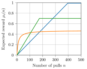
(a)

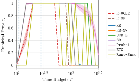
(b)

Figure 6: Challenging scenario in which the arm reward increment rate changes abruptly.

F.2 Sensitivity Analysis on the Noise Variance

In what follows, we report the analysis of the robustness of the analyzed algorithms as noise standard deviation $\sigma$ changes in the collected samples. The setting we considered is the one described in Section 8. The results are provided in Figure 7. Let us focus on the performances of the R-UCBE algorithm. For small values of the standard deviation ($\sigma<0.01$), we have the same behavior in terms of error probability, i.e., a progressive degradation of the performances for time budget $T=150$. Indeed, at this time budget, the expected rewards of $3$ arms are close to each other, and determining the optimal arm is a challenging problem. However, the performances are better or equal to all the other algorithms even at this point. Conversely, for values of the standard deviation $\sigma\geq 0.05$, the performance of R-UCBE starts to degrade, with behavior for $\sigma=0.5$ which is constant w.r.t. the chosen time budget with a value of $\overline{e}_{T}(\text{{R-UCBE}\@})=0.8$. This suggests that such an algorithm suffers in the case the stochasticity of the problem is significant. Let us focus on R-SR. This algorithm does not change its performances w.r.t. changes in terms of $\sigma$. Indeed, only for $\sigma=0.5$, we have that it does not provide an error probability close to zero for time budget $T>1000$. However, excluding R-UCBE, we have that the R-SR algorithm is the best/close to the best performing algorithm. This is also true in the case of $\sigma=0.5$, in which the R-UCBE fails in providing a reliable recommendation for the optimal arm with a large probability.

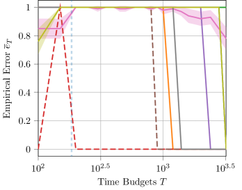
(a)

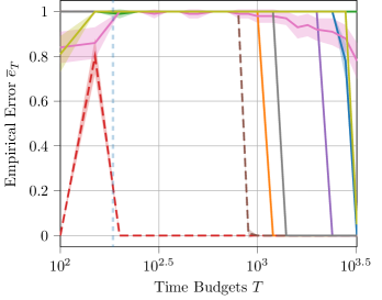
(b)

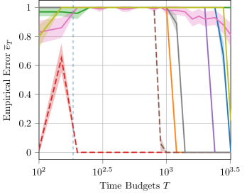
(c)

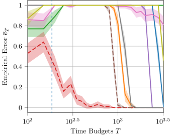
(d)

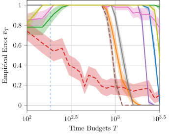
(e)

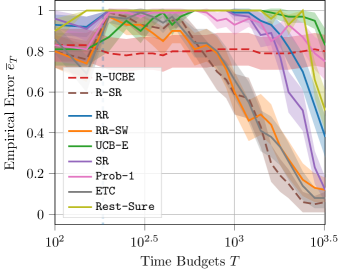
(f)

Figure 7: Empirical error probability for the synthetically generated setting, with different values of the noise standard deviation $\sigma$.

F.3 Real-world Experiment on IMDB dataset

Description  We validate our algorithms and the baselines on an AutoML task, namely an online best model selection problem with a real-world dataset. We employ the IMDB dataset, made of $50,000$ reviews of movies (scores from $0$ to $10$). We preprocessed the data as done by Metelli et al. [2022], and run the algorithms for time budgets $T\in\mathcal{T}\coloneqq\{500,1000,\ldots,15000,20000,30000\}$. A graphical representation of the reward (in this case, represented by the accuracy) of the different models is presented in Figure 8. Since, in this case, we only had a single realization to estimate the error probability $\bar{e}_{T}(\mathfrak{A})$, we report the success rate $R(\mathfrak{A})$ instead, i.e., the ratio between the number of times an algorithm provides a correct suggestion and the number of budget values we considered, formally defined as $R(\mathfrak{A})\coloneqq\frac{1}{|\mathcal{T}|}\sum_{T\in\mathcal{T}}\mathds{1}\{\hat{I}^{*}=i^{*}\}$ (the larger, the better).

Results  The results are reported in Table 3. The algorithm with the largest success rate $R(\mathfrak{U})$ is the R-UCBE, while R-SR provides the third best success rate. Moreover, Rest-Sure, the only algorithm providing a success rate larger than R-SR, has issues with large time budgets since for $T\geq 5000$ is able to provide only $2$ correct guesses of the optimal arm over $6$ attempts. Conversely, our algorithms progressively provide more and more correct guesses as the time budget $T$ increases. The above results on a real-world dataset corroborate the evidence presented above that the proposed algorithms outperform state-of-the-art ones for the BAI problem in SRB.

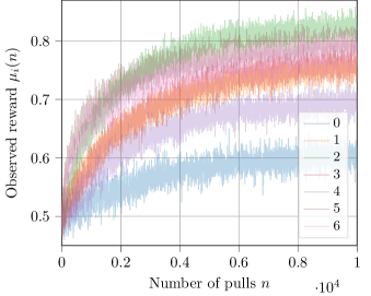
Figure 8: Rewards for the arms of the IMDB experiments.

			$T$										$R(\mathfrak{U})$
		$500$	$1000$	$2000$	$3000$	$4000$	$5000$	$7000$	$10000$	$15000$	$20000$	$30000$
	Optimal Arm	$5$	$5$	$2$	$2$	$2$	$2$	$2$	$2$	$2$	$2$	$2$
Algorithms	R-UCBE (ours)	$6$	$5$	$2$	$5$	$2$	$2$	$2$	$2$	$2$	$2$	$2$	$9/11$
	R-SR (ours)	$5$	$5$	$5$	$5$	$5$	$5$	$5$	$5$	$2$	$2$	$2$	$5/11$
	RR	$5$	$5$	$5$	$5$	$5$	$5$	$5$	$5$	$5$	$5$	$5$	$2/11$
	RR-SW	$5$	$5$	$5$	$5$	$5$	$5$	$5$	$5$	$5$	$2$	$2$	$4/11$
	SR	$5$	$5$	$5$	$5$	$5$	$5$	$5$	$5$	$5$	$5$	$2$	$3/11$
	UCB-E	$5$	$5$	$5$	$5$	$5$	$5$	$5$	$5$	$5$	$5$	$5$	$2/11$
	Prob-1	$1$	$5$	$2$	$5$	$5$	$5$	$5$	$1$	$5$	$6$	$2$	$3/11$
	ETC	$5$	$5$	$5$	$5$	$5$	$5$	$5$	$5$	$5$	$5$	$2$	$3/11$
	Rest-Sure	$6$	$5$	$2$	$2$	$2$	$1$	$0$	$2$	$5$	$0$	$2$	$6/11$

Table 3: Optimal arm for different time budgets on the IMDB dataset (first row) and corresponding recommendations provided by the algorithms (second to last row). In the last column, we compute the corresponding success rate.

References

- Lattimore and Szepesvári [2020] Tor Lattimore and Csaba Szepesvári. Bandit algorithms. Cambridge University Press, 2020.
- Auer et al. [2002] Peter Auer, Nicolo Cesa-Bianchi, and Paul Fischer. Finite-time analysis of the multiarmed bandit problem. Machine Learning, 47(2):235–256, 2002.
- Bubeck et al. [2009] Sébastien Bubeck, Rémi Munos, and Gilles Stoltz. Pure exploration in multi-armed bandits problems. In Proceedings of the Algorithmic Learning Theory (ALT), volume 5809, pages 23–37, 2009.
- Tekin and Liu [2012] Cem Tekin and Mingyan Liu. Online learning of rested and restless bandits. IEEE Transaction on Information Theory, 58(8):5588–5611, 2012.
- Metelli et al. [2022] Alberto Maria Metelli, Francesco Trovò, Matteo Pirola, and Marcello Restelli. Stochastic rising bandits. In Proceedings of the International Conference on Machine Learning (ICML), pages 15421–15457, 2022.
- Thornton et al. [2013] Chris Thornton, Frank Hutter, Holger H Hoos, and Kevin Leyton-Brown. Auto-weka: Combined selection and hyperparameter optimization of classification algorithms. In Proceedings of the ACM (SIGKDD), pages 847–855, 2013.
- Kotthoff et al. [2017] Lars Kotthoff, Chris Thornton, Holger H Hoos, Frank Hutter, and Kevin Leyton-Brown. Auto-weka 2.0: Automatic model selection and hyperparameter optimization in weka. Journal of Machine Learning Research, 18:1–5, 2017.
- Erickson et al. [2020] Nick Erickson, Jonas Mueller, Alexander Shirkov, Hang Zhang, Pedro Larroy, Mu Li, and Alexander Smola. Autogluon-tabular: Robust and accurate automl for structured data. arXiv preprint arXiv:2003.06505, 2020.
- Li et al. [2020] Yang Li, Jiawei Jiang, Jinyang Gao, Yingxia Shao, Ce Zhang, and Bin Cui. Efficient automatic CASH via rising bandits. In Proceedings of the Conference on Artificial Intelligence (AAAI), pages 4763–4771, 2020.
- Zöller and Huber [2021] Marc-André Zöller and Marco F Huber. Benchmark and survey of automated machine learning frameworks. Journal of Artificial Intelligence Research, 70:409–472, 2021.
- Feurer et al. [2015] Matthias Feurer, Aaron Klein, Katharina Eggensperger, Jost Tobias Springenberg, Manuel Blum, and Frank Hutter. Efficient and robust automated machine learning. In Advances in Neural Information Processing Systems (NeurIPS), pages 2962–2970, 2015.
- Yao et al. [2018] Quanming Yao, Mengshuo Wang, Yuqiang Chen, Wenyuan Dai, Yu-Feng Li, Wei-Wei Tu, Qiang Yang, and Yang Yu. Taking human out of learning applications: A survey on automated machine learning. arXiv preprint arXiv:1810.13306, 2018.
- Hutter et al. [2019] Frank Hutter, Lars Kotthoff, and Joaquin Vanschoren. Automated machine learning: methods, systems, challenges. Springer Nature, 2019.
- Mussi et al. [2023] Marco Mussi, Davide Lombarda, Alberto Maria Metelli, Francesco Trovó, and Marcello Restelli. Arlo: A framework for automated reinforcement learning. Expert Systems with Applications, 224:119883, 2023.
- Cella et al. [2021] Leonardo Cella, Massimiliano Pontil, and Claudio Gentile. Best model identification: A rested bandit formulation. In Proceedings of the International Conference on Machine Learning (ICML), volume 139, pages 1362–1372, 2021.
- Heidari et al. [2016] Hoda Heidari, Michael J. Kearns, and Aaron Roth. Tight policy regret bounds for improving and decaying bandits. In Proceeding of the International Joint Conference on Artificial Intelligence (AISTATS), pages 1562–1570, 2016.
- Lehmann et al. [2001] Benny Lehmann, Daniel Lehmann, and Noam Nisan. Combinatorial auctions with decreasing marginal utilities. In ACM Proceedings of the Conference on Electronic Commerce (EC), pages 18–28, 2001.
- Audibert et al. [2010] Jean-Yves Audibert, Sébastien Bubeck, and Rémi Munos. Best arm identification in multi-armed bandits. In Proceedings of the Conference on Learning Theory (COLT), pages 41–53, 2010.
- Heide et al. [2021] Rianne De Heide, James Cheshire, Pierre Ménard, and Alexandra Carpentier. Bandits with many optimal arms. In Advances in Neural Information Processing Systems (NeurIPS), pages 22457–22469, 2021.
- Kaufmann et al. [2016] Emilie Kaufmann, Olivier Cappé, and Aurélien Garivier. On the complexity of best-arm identification in multi-armed bandit models. Journal of Machine Learning Research, 17:1:1–1:42, 2016.
- Gabillon et al. [2012] Victor Gabillon, Mohammad Ghavamzadeh, and Alessandro Lazaric. Best arm identification: A unified approach to fixed budget and fixed confidence. In Advances in Neural Information Processing Systems (NeurIPS), pages 3221–3229, 2012.
- Abbasi-Yadkori et al. [2018] Yasin Abbasi-Yadkori, Peter L. Bartlett, Victor Gabillon, Alan Malek, and Michal Valko. Best of both worlds: Stochastic & adversarial best-arm identification. In Proceedings of the Conference on Learning Theory (COLT), volume 75, pages 918–949, 2018.
- Garivier and Kaufmann [2016] Aurélien Garivier and Emilie Kaufmann. Optimal best arm identification with fixed confidence. In Proceedings of the Conference on Learning Theory (COLT), volume 49, pages 998–1027, 2016.
- Carpentier and Locatelli [2016] Alexandra Carpentier and Andrea Locatelli. Tight (lower) bounds for the fixed budget best arm identification bandit problem. In Proceedings of the 29th Conference on Learning Theory, volume 49, pages 590–604, 2016.
- Mintz et al. [2020] Yonatan Mintz, Anil Aswani, Philip Kaminsky, Elena Flowers, and Yoshimi Fukuoka. Nonstationary bandits with habituation and recovery dynamics. Operations Research, 68(5):1493–1516, 2020.
- Seznec et al. [2020] Julien Seznec, Pierre Ménard, Alessandro Lazaric, and Michal Valko. A single algorithm for both restless and rested rotting bandits. In Proceedings of the International Conference on Artificial Intelligence and Statistics (AISTATS), volume 108, pages 3784–3794, 2020.
- Levine et al. [2017] Nir Levine, Koby Crammer, and Shie Mannor. Rotting bandits. In Advances in Neural Information Processing Systems (NeurIPS), pages 3074–3083, 2017.
- Seznec et al. [2019] Julien Seznec, Andrea Locatelli, Alexandra Carpentier, Alessandro Lazaric, and Michal Valko. Rotting bandits are no harder than stochastic ones. In Proceedings of the International Conference on Artificial Intelligence and Statistics, volume 89, pages 2564–2572, 2019.