Self-Supervised Temporal Graph Learning with Temporal and Structural Intensity Alignment

Abstract

Temporal graph learning aims to generate high-quality representations for graph-based tasks along with dynamic information, which has recently drawn increasing attention. Unlike the static graph, a temporal graph is usually organized in the form of node interaction sequences over continuous time instead of an adjacency matrix. Most temporal graph learning methods model current interactions by combining historical information over time. However, such methods merely consider the first-order temporal information while ignoring the important high-order structural information, leading to sub-optimal performance. To solve this issue, by extracting both temporal and structural information to learn more informative node representations, we propose a self-supervised method termed S2T for temporal graph learning. Note that the first-order temporal information and the high-order structural information are combined in different ways by the initial node representations to calculate two conditional intensities, respectively. Then the alignment loss is introduced to optimize the node representations to be more informative by narrowing the gap between the two intensities. Concretely, besides modeling temporal information using historical neighbor sequences, we further consider the structural information from both local and global levels. At the local level, we generate structural intensity by aggregating features from the high-order neighbor sequences. At the global level, a global representation is generated based on all nodes to adjust the structural intensity according to the active statuses on different nodes. Extensive experiments demonstrate that the proposed method S2T achieves at most 10.13% performance improvement compared with the state-of-the-art competitors on several datasets.

I Introduction

Graph learning has drawn increasing attention [1, 2], since more and more real-world scenarios can be present as graphs, such as web graphs, social graphs, and citation graphs [3, 4, 5, 6]. Traditional graph learning methods are based on static graphs, and they usually use adjacency matrices to generate node representations by aggregating neighborhood features [7, 8, 9, 10]. Unlike static graphs, a temporal graph is organized in the form of node interaction sequences over continuous time instead of an adjacency matrix. In the real world, many graphs contain node interactions with timestamps. Capturing the time information and combining them into node representations is important for models to predict future interactions.

It is worth noting that temporal graph-based methods can hardly generate node representations directly using the adjacency matrix to aggregate neighbor information like a static graph-based method [11, 12]. Due to the special data form of the temporal graph that sorts node interactions by time, temporal methods are trained in batches of data [13]. Thus these methods typically store neighbors in interaction sequences and model future interactions from historical information. However, such temporal methods merely consider the first-order temporal information while ignoring the important high-order structural information, leading to sub-optimal performance.

To solve this issue, by extracting both Temporal and structural information to learn more informative node representations, we propose a Self-Supervised method termed S2T for Temporal graph learning. Note that the first-order temporal information and the high-order structural information are combined in different ways by the initial node representations to calculate two conditional intensities, respectively. Then the alignment loss is introduced to optimize the node representations to be more informative by narrowing the gap between the two intensities. More specially, for temporal information modeling, we leverage the Hawkes process [14] to calculate the temporal intensity between two nodes. Besides considering the two nodes’ features, the Hawkes process also considers the effect of their historical neighbors on their future interactions.

On the other hand, we further extract the structural information, which can be divided into the local and global level. When capturing the local structural information, we first utilize GNN to generate node representations by aggregating the high-order neighborhood features. After that, the global structural information is extracted to enhance long-tail nodes. In particular, a global representation generated based on all nodes is proposed, which is used to update node representations according to active statuses on different nodes. After the structural intensity is calculated based on node representations, we also construct a global parameter to assign importance weights for different dimensions of the structural intensity vector. Finally, in addition to the task loss, we utilize the alignment loss to narrow the gap between the temporal and structural intensity vectors and impose constraints on global representation and parameters, which constitute the total loss function.

We conduct extensive experiments to compare our method S2T with the state-of-the-art competitors on several datasets, the results demonstrate that S2T achieves at most 10.13% performance improvement. Furthermore, the ablation and parameter analysis shows the effectiveness of our model.

In conclusion, the contributions are summarized as follows:

(1) We extract both temporal and structural information to obtain different conditional intensities and introduce the alignment loss to narrow their gap for learning more informative node representations.

(2) To enhance the information on the long-tail nodes, we capture the global structural information as an augmentation of the local structural module.

(3) We compare S2T with multiple methods in several datasets and demonstrate the performance of our method.

II Related Work

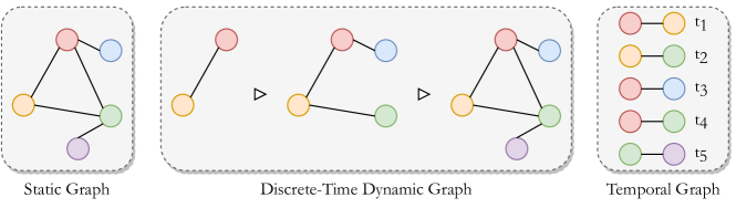
Figure 1: Different graphs: static, discrete, and temporal.

Graph Learning is an important technology which can be used for many fields, such as interest recommendation [15, 16], biological informatics [17, 18], knowledge graph [19, 20], and community detection [21, 22], etc. Generally, graph data can be divided into static graph data and dynamic graph data. The most essential difference between them is whether the data contains interaction time information [23, 24, 25].

As shown in Fig. 1, we discuss the different types of graph data here. Traditional graph learning methods learn node representations on static graphs, which focus on the graph topology [26]. In these graphs, nodes and edges will not change, and there is no concept of time [27].

To name a few, DeepWalk [28] performs random walks over the graph to learn node embeddings (also called representations). node2vec [29] conducts random walks on the graph using breadth-first and depth-first strategies to balance neighborhood information of different orders. VGAE [30] migrates variational auto-encoders to graph data and use encoder-decoder module to reconstruct graph information. GraphSAGE [31] leverages an aggregation function to sample and combine features from a node’s local neighborhood.

In addition, many real-world data contain dynamic interactions, thus graph learning methods based on dynamic graphs are becoming popular [32, 33, 22]. Concretely, dynamic graphs can also be divided into discrete graphs (also called discrete-time dynamic graphs, DTDG) and temporal graphs (also called continuous-time dynamic graphs, CTDG).

A discrete graph usually contains multiple static snapshots, each snapshot is a slice of the interaction of the graph whole graph at a certain timestamp, which can be regarded as a static graph. When multiple snapshots are combined, there is a time sequence among them. Because each static snapshot is computationally equivalent to that of a static graph, which makes the computation significantly less efficient, only a small amount of work is performed on discrete graphs. Such as EvolveGCN [34] uses the RNN model to update the parameters of GCN for future snapshots. DySAT [35] combines graph structure and dynamic information to generate self-weighted node representations.

Unlike discrete graphs, a temporal graph no longer observes graph evolution over time from a macro perspective but focuses on each node interaction. For example, CTDNE [36] performs a random walk on graphs to model temporal ordered sequences of node walks. HTNE [37] is the first to utilize the Hawkes process to model historical events on temporal graphs. MMDNE [38] models graph evolution over time from both macro and micro perspectives. TGAT [39] replaces traditional modeling form of self-attention with interaction temporal encoding. MNCI [40] mines community and neighborhood influences to generate node representations inductively. TREND [41] replaces the Hawkes process with GNN to model the temporal information.

Although the effectiveness of all these methods mentioned above has been proven, they only consider one-order temporal information or high-order structural information, and the performance can be further improved. To our knowledge, integrating both types of information is still an open problem, thus we propose the S2T method to solve it. In the following, we discuss S2T in detail how it maintains a balance between temporal and structural information.

III Method

In this part, we first introduce the overall framework of S2T and then denote some preliminaries. After that, we describe each component module in detail.

III-A Overall Framework

As shown in Figure 2, our method S2T can be divided into several main parts: temporal information modeling, structural information modeling, and loss function, where a local module and a global module work together to realize structural information modeling. Then the alignment loss is introduced into the loss function, which aligns temporal and structure information.

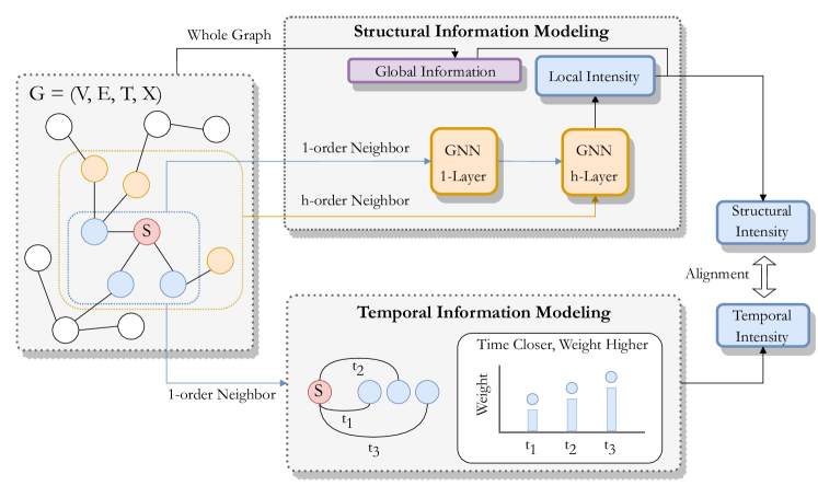
Figure 2: Overall Framework of S2T. In the structural information modeling part, we leverage GNN to calculate local intensity by aggregating multi-order neighbor features. Such intensity is further enhanced by the global information into the structural intensity. In the temporal information modeling part, we utilize the Hawkes process to calculate the temporal intensity by modeling the one-order neighbor sequence. Finally, we introduce the alignment loss into the loss function to narrow the semantic gap between the two intensity vectors.

III-B Preliminaries

First, we define the temporal graph based on the timestamps accompanying the node interactions.

Definition 1

Temporal Graph. Given a temporal graph $G=(V,E,T,X)$, where $V$ and $E$ denote the set of nodes and edges (called interactions here), $T$ denotes the timestamp set of node interactions, and $X$ denotes the node features. If an edge exists between node $x$ and $y$, this means that they have interacted at least once, i.e., $T_{x,y}=\{(x,y,t_{1}),(x,y,t_{2}),\cdots,(x,y,t_{n})\}$.

When two nodes interact, we call them neighbors. Note that in temporal graphs, the concept of interaction replaces the concept of edges, and multiple interactions can occur between two nodes.

Definition 2

Historical Neighbor Sequence. For each node $x$, there will be a historical neighbor sequence $N_{x}$, which stores all interactions of $x$, i.e., $N_{x}=\{(y_{1},t_{1}),(y_{2},t_{2}),\cdots,(y_{n},t_{n})\}$.

In a temporal graph, one interaction data is stored as a tuple of $(x,y,t)$, which means that the two nodes $x$ and $y$ interact at time $t$. In the actual training, we feed these interaction data into the model in batches. Our objective is to conduct a mapping function $F$ that converts high-dimensional sparse graph-structured data $G$ into low-dimensional dense node representations $Z$.

The descriptions of notations is shown in Table I.

TABLE I: Notations.

Notation	Description
$z_{x},z_{y}$	Node representations of node $x$ and $y$
$N_{x},N_{y}$	Neighborhood sequences of node $x$ and $y$
$\lambda^{T}_{(x,y)}(t),\lambda^{S}_{(x,y)}(t)$	Temporal and structural conditional intensity for interaction $(x,y,t)$
$\mu_{(x,y)}$	Base intensity between node $x$ and $y$ without any external influence
$\alpha_{(x,y)}$	Used to calculate the Hawkes intensity
$s_{(x,y)},f(t_{c}-t_{i})$	Similarity and temporal weights, which are combined to give $\alpha_{(x,y)}$
$z_{g},g_{g}^{t}$	Global representation and its update weight
$\alpha^{(x,y,t)},\beta^{(x,y,t)}$	Global parameter: scaling and shifting operators for interaction $(x,y,t)$
$L_{task},L_{A},L_{G}$	Task loss, alignment loss, and global prameter loss

III-C Temporal Information Modeling

To maintain the paper’s continuity, we first introduce the temporal module and then introduce the structural module.

Given two nodes $x$ and $y$, we can indicate the likelihood of their interaction by calculating the conditional intensity between them. There are two ways to obtain it, here we discuss the first way: modeling temporal information with the Hawkes process [14]. Such a point process considers a node’s historical neighbors will influence the node’s future interactions, and this influence decays over time.

Define $z_{x}$ and $z_{y}$ to denote the representations of node $x$ and $y$ respectively, which is obtained by a simple linear mapping of their features. Their temporal interaction intensity $\lambda^{T}_{(x,y)}(t)$ can be calculated as follows,

$$\lambda^{T}_{(x,y)}(t)=\mu_{(x,y)}+\sum_{i\in N_{x}}\alpha_{(i,y)}\mu_{(i,y)}+\sum_{i\in N_{y}}\alpha_{(i,x)}\mu_{(i,x)},$$ (1)

$$\mu_{(x,y)}=-||z_{x}-z_{y}||^{2},\quad\alpha_{(i,y)}=s_{(i,x)}\cdot f(t_{c}-t_{i}).$$ (2)

This intensity can be divided into two parts: (1) the first part is the base intensity between two nodes without any external influence, i.e., $\mu_{(x,y)}$; (2) the second part is the Hawkes intensity that focuses on how a node’s neighbors influence another node, where $i$ denotes the neighbor in the sequence, i.e., $\sum_{i\in N_{x}}\alpha_{(i,y)}\mu_{(i,y)}$.

In the Hawkes intensity, $\alpha_{(i,y)}$ measures the influence of a single neighbor node $i$ of $x$ on $y$, and this influence is weighted by two aspects. On the one hand, $s_{(i,x)}$ is the similarity weight between neighbor $i$ and source node $x$ in the neighbor sequence $N_{x}$, i.e., $s_{(i,x)}=\frac{\exp(\mu_{(i,x)})}{\sum_{i^{\prime}\in N_{x}}\exp(\mu_{(i^{\prime},x)})}$. This similarity weight means that although we calculate the influence of each neighbor $i$ in $N_{x}$ on $y$, we also need to consider the corresponding weights $s_{(i,x)}$ for different $i$ in $N_{x}$. Note that in the Hawkes intensity, both $\mu_{(i,y)}$ and $\mu_{(i,x)}$ appear, and their roles are different. On the other hand, the function $f(t_{c}-t_{i})$ considers the interaction time interval between $i$ and $x$, i.e., $f(t_{c}-t_{i})=\exp(-\delta_{t}(t_{c}-t_{i}))$, where $\delta_{t}$ is a learnable parameter. In this function, neighbors that interact closer to the current time $t_{c}$ are given more weight.

In addition, the total number of neighbors may vary from node to node. In actual training, if we obtain all of its neighbors for each node, the computational pattern of each batch can not be fixed, which brings great computational inconvenience. Referencing previous works [37, 42, 43, 41] and our experiments, we fix the sequence length $S$ of node neighbors and select the latest $S$ neighbors for each node at each timestamp instead of full neighbors. In Section IV, we will discuss the sensitivity of the hyper-parameter $S$ in experiments.

III-D Local Structural Information Modeling

In addition to the Hawkes process, the GNN model can also be used to calculate conditional intensity. Unlike the Hawkes process which focuses on the temporal information of the first-order neighbors, GNN is more concerned with aggregating information about the high-order neighbors. For each node $x$ at time $t$, we construct $l$ GNN layers to generate its representation $z_{x}^{t,l}$ as follows,

$$z_{x}^{t,l}=\sigma(z_{x}^{(t,l-1)}W_{S}^{l}+\sum_{i\in N_{x}}z_{i}^{(t_{i},l-1)}W_{N}^{l}\odot k(t_{c}-t_{i})),$$ (3)

$$k(t_{c}-t_{i})=\frac{t_{c}-t_{i}}{\sum_{i^{\prime}\in N_{x}}t_{c}-t_{i^{\prime}}},$$ (4)

where $W_{S}^{l}$ and $W_{N}^{l}$ are learnable parameters, $\odot$ denotes element-wise multiplication, $\sigma$ is the sigmoid function, and $k(t_{c}-t_{i})$ is used to generate normalized weights for the interaction time intervals of different neighbors. The first layer’s input $h_{x}^{t,0}$ is a simple linear mapping of node features, and the final layer’s output $h_{x}^{t,l}$ is the aggregated representation containing the $l$-order neighborhood information. Note that both Hawkes intensity and GNN intensity utilize the original linear mapping representations as input, and we utilize generate representations based on GNN as the final output.

Given two nodes, their local conditional intensity measures how similar the information they aggregated is, which can be calculated as follows,

$$\lambda^{S}_{(x,y)}(t)=-||z_{x}^{t}-z_{y}^{t}||^{2}\odot\omega_{g},$$ (5)

where $\omega_{g}$ is a global parameter that will be described below.

III-E Global Structural Information Modeling

After calculating the node representations based on GNN, we construct a global module to enhance the structural information modeling. Firstly, let us discuss why we need information enhancement.

In most graphs, there are always a large number of long-tail nodes that interact infrequently but are the most common in the graph. Due to their limited interactions, it is hard to find sufficient data to generate their representations. Previous works usually aggregate high-order neighbor information to enhance their representations, which is consistent with the purpose of our GNN module above. But in addition, we worry that too much external high-order information will dominate instead, bringing unnecessary noise to long-tail nodes. Therefore, we generate a global representation that provides partial basic information for these nodes.

III-E1 Global Representation

Global representation, as an abbreviated expression for the whole graph environment, is updated based on all nodes. In the graph, only a small number of nodes are high-active due to their large number of interactions that influence the graph evolution, while most long-tail nodes are vulnerable to the whole graph environment. Using global representation to fill basic information for long-tail nodes can ensure their representations are more suitable for unsupervised scenarios.

Here we introduce the concept of node active status from the LT model [44] in the information propagation field [45, 46]. A node’s active status varies with its interaction frequency and can be used to measure how active a node is in the global environment. To be specific, the node active status can be used in two parts: (1) control the update of the global representation; (2) control the weight of global representation providing information to nodes.

For the first part, the global representation $z_{g}$ doesn’t contain any information when it is initialized, and it needs to be updated by nodes. Note that in a temporal graph, nodes are trained in batches according to the interaction order. When a batch of nodes is fed into the model, the global representation can be updated as follows,

$$z_{g}:=z_{g}+g_{g}^{t}\odot z_{x}^{t},\quad g_{g}^{t}=\theta_{d}\cdot|N_{x}^{t}|.$$ (6)

In this equation, $\theta_{d}$ is a learnable parameter. $|N_{x}^{t}|$ is the number of neighbors that node $x$ interacts with at time $t$ and we call it node dynamics here. $g_{g}^{t}$ determines how much $x$ updates the global representation. In general, the more active a node $x$ is, the more influence it has on the global environment, so its corresponding weight $g_{g}^{t}$ is larger.

For the second part, the global representation is generated to enhance the long-tail nodes, thus it needs to add to the node representations. In contrast, the less active a node is, the more basic information it needs from the global representation. As for nodes with high active status, they have a lot of interactive information and do not need much data enhancement. Thus the update of node representations can be formed as follows,

$$z_{x}^{t}:=z_{x}^{t}+g_{x}^{t}\odot z_{g},\quad g_{x}^{t}=\theta_{d}/|N_{x}^{t}|.$$ (7)

Compared to Eq. 6, the same parameter $\theta_{d}$ is used in Eq. 7, while the node dynamics are set to the reciprocal, i.e., $1/|N_{x}^{t}|$. In one batch training, we first update the global representation, and then update the representation. The specific training flow is shown in Algorithm. 1.

By enhancing the long tail nodes, the model can learn more reliable node representations. The more long-tail nodes in a graph, the more obvious the effect is, which is demonstrated in the following experiment subsection IV-D.

III-E2 Global Parameter

As mentioned in Eq. (5), after calculating the local intensity, we also construct a global parameter $\omega_{g}$ to assign importance weights for different dimensions of the intensity vector $\lambda^{S}_{x,y}(t)$. More specially, this global parameter can fine adjust the different dimensions of conditional intensity through a set of scaling and shifting operations so that those dimensions that are more likely to reflect node interaction are amplified. We first construct a simple learnable parameter $\theta_{l}$ , and then leverage the Feature-wise Linear Modulation (FiLM) layer [47] to construct $\omega_{g}$,

$$\omega_{g}=(\alpha^{(x,y,t)}+1)\cdot\theta_{l}+\beta^{(x,y,t)},$$ (8)

$$\alpha^{(x,y,t)}=\sigma(W_{\alpha}\cdot(z_{x}^{t}||z_{y}^{t})+b_{\alpha}),$$ (9)

$$\beta^{(x,y,t)}=\sigma(W_{\beta}\cdot(z_{x}^{t}||z_{y}^{t})+b_{\beta}).$$ (10)

FiLM layer consists two parts: a scaling operator $\alpha^{(x,y,t)}$ and a shifting operator $\beta^{(x,y,t)}$, where $W_{\alpha}$, $b_{\alpha}$, $W_{\beta}$, $b_{\beta}$ are learnable parameters. Note that parameter enhancement by combining node representations allows the new parameters $\omega_{g}$ to better understand the meaning of each dimension of node representations. In this way, the parameter can finely adjust the importance of the different dimensions of the intensity vector, so that the conditional intensity can better reflect the possibility of node interaction.

III-F Loss Function

III-F1 Task Loss

The local conditional intensity calculated above is used to construct the classic loss function for link prediction [48] and we utilize the GNN-based node representations as final input into the loss function $L_{task}$ as follows,

$$L_{task}=-\log\sigma(\lambda^{S}_{(x,y)}(t))-\sum_{k\sim P_{x}}\log\sigma(1-\lambda^{S}_{(x,k)}(t)).$$ (11)

In this loss function, we introduce the negative sampling technology [49] to generate the positive pair and negative pair. The positive pair contains nodes $x$ and $y$, their local intensity can be used to measure how likely they are to interact. For the negative pair, we introduce the negative sampling technology to obtain samples randomly. $P_{x}$ is the negative sample distribution, which is proportional to node $u$’s degree. In this way, we constrain the positive sample intensity to be as large as possible and the negative sample intensity to be as small as possible.

III-F2 Alignment Loss

Note that we do not utilize the node representations from the temporal module as the final output because they are simple mappings of node origin features. Such node representations are used only to model temporal information as a complement to the structural information. To achieve this goal, we leverage the alignment loss the constrain the temporal intensity $\lambda^{T}$ and $\lambda^{S}$ to be as close as possible, thus constraining the temporal information as a complement to the structural information. It means that these two intensities can be compared to each other, thereby guiding the model to strike a balance between different information preferences. Here we utilize the Smooth $L1$ loss to measure it,

$$L_{A}=Smooth(\lambda^{T},\lambda^{S}).$$ (12)

Denote $\lambda^{T}-\lambda^{S}$ as $\Delta\lambda$, the Smooth $L1$ loss can be formulated as follows,

$$Smooth(\lambda^{T},\lambda^{S})=\begin{cases}\frac{1}{2}(\Delta\lambda)^{2},&\text{$|\Delta\lambda|<1$}\\ |\Delta\lambda|-\frac{1}{2},&\text{$|\Delta\lambda|\geq 1$}.\end{cases}$$ (13)

III-F3 Global Loss

For the global representation and global parameters in this module, we construct a loss function $L_{G}$ to constrain their variation,

$$L_{G}=\log\sigma(-||z_{x}^{t}-z_{g}||^{2}-||z_{y}^{t}-z_{g}||^{2})+||\alpha||^{2}+||\beta||^{2}.$$ (14)

Among them, the global representation should be as similar to the node representation as possible to maintain its smoothness, and the global parameter should be as close to $0$ as possible. In this way, we can ensure the global parameter’s finely adjusting ability because its values are constrained to transform in a small range.

III-F4 Total Loss

The total loss function contains several parts: the task loss $L_{task}$, the alignment loss $L_{A}$, and the global loss $L_{G}$. According to Eq. (11), (12), and (14), the total loss function $L$ can be formally defined as follows,

$$L=L_{task}+\eta_{1}L_{A}+\eta_{2}L_{G},$$ (15)

where $\eta_{1}$ and $\eta_{2}$ are learnable parameters used to weigh the constraint of alignment loss and global loss. In general, these two parameters should be set as hyper-parameters and fine-tuned according to the experimental results. But we found that setting it as a learnable parameter was equally effective and more flexible, minimizing the frequency of manual intervention by researchers.

III-G Complexity Analysis

To analysis the time complexity of S2T, we first given its pseudo-code shown in Algorithm. 1.

Algorithm 1 S2T procedure

0:  Temporal graph $G=(V,\ E,\ T,\ X)$.

0:  Node representations.

1:  Initialize global representation $z_{g}$ and parameters;

2:  Split $G$ in batches;

3:  repeat

4:     for each $batch$ do

5:        Calculate node representations based on Eq. (3);

6:        Update global representation $z_{g}$ based on Eq. (6);

7:        Update node representations based on Eq. (7);

8:        Calculate global parameter $\omega_{g}$ based on Eq. (8);

9:        Calculate $\lambda^{S}_{(x,y)}(t)$ based on Eq. (5);

10:        Calculate $\lambda^{T}_{(x,y)}(t)$ based on Eq. (1);

11:        Optimize the loss function based on Eq. (15);

12:     end for

13:  until Convergence

Let $|E|$ be the number of edges, $t$ be the number of epochs, $d$ be the representation size, $l$ be the number of GNN layers, $S$ be the length of the historical neighbor sequence, and $Q$ be the number of negative sample nodes.

According to Algorithm. 1, we can discuss the time complexity by line:

1. Lines 1-2. The complexity of initialization of the parameters depends on the largest size parameter, here it is $O(d^{2})$. Splitting graph by batches is equivalent to traversing the graph, whose complexity is denoted as $O(|E|)$.

2. Line 5. The computation of node representation based on GNN is related to the number of layers and the number of neighbors. The complexity of the representation of the previous layer is converted to $O(d^{2})$, and the complexity of computing domain information of the current layer is $O(S^{2}d^{2})$. Consider the number of layers, the complexity of this part is $O(lS^{2}d^{2})$.

3. Lines 6-7. For each node, the updating of global representation and node representation have the same complexity, i.e., $O(d)$.

4. Line 8. The complexity of calculating global parameter needs to consider the structure of FiLM layer, which can be denoted as $O(d^{2})$.

5. Lines 9-11. The optimization of the loss function is divided into two steps. Firstly, the results of each part of the loss function are calculated by forward propagation, and then the model parameters are optimized by back propagation. The complexity of forward propagation is $O(QS^{3}d^{3})$, the complexity of back propagation is $O(d^{2})$.

Considering the number of epochs $t$ and edges $|E|$ outside of the loop, its time complexity can be formalized as follows,

$$O(d^{2}+|E|+t|E|(lS^{2}d^{2}+d+d^{2}+QS^{3}d^{3}+d^{2}))$$ (16)

$$=O(t|E|(lS^{2}d^{2}+QS^{3}d^{3})).$$

Because $l,S,Q$ are all small constants, thus the time complexity of S2T can be simplified as $O(t|E|d^{3})$.

III-H Discussion

III-H1 Inductive Learning

S2T can handle new nodes and edges as well, and it is an implicitly inductive model. For a new node-interaction join, we only need to obtain its features and interaction neighbors to generate its node representations from readily available GNNs and global representations. Note that S2T processes the temporal graph data in batches, and each batch of data is equivalent to new nodes and interactions for it, so it is inherently inductive. In fact, almost all temporal models are natural inductive learning models.

III-H2 Information Complementary Analysis

In this part, we discuss the information complementary of the three modules: temporal information modeling, local structural information modeling, and global structural information modeling. Here we measure the modeling scope of different modules by node sequences. Given a node $x$, its one-order neighbors can be defined as $N_{x}^{1}$. The temporal module’s scope is equal to it, i.e., $S_{t}=\{N_{x}^{1}\}$, because the module only focuses on the one-order neighbor sequence.

The local structural module further pays attention to high-order neighbors based on GNN, thus the number of GNN layers can be used to evaluate the order of neighborhood. In this way, the module’s scope can be formulated as $S_{l}=\{N_{x}^{1}+N_{x}^{2}+\cdots+N_{x}^{l}\}$. The global structural module captures information over the whole graph and each node in the graph will be used to update the global representation and parameter, thus the global module’s scope can be formulated as $S_{g}=\{V\}$.

In terms of the modeling scope, the temporal module’s scope is contained in the local module, which in turn is contained in the global module, i.e., $\{N_{x}^{1}\}\in\{N_{x}^{1}+N_{x}^{2}+\cdots+N_{x}^{l}\}\in\{V\}$. And in terms of modeling depth, the temporal graph module digs the deepest information, while the global module digs the shallowest. This combination of models is logical. In a graph, the most likely to influence a node is its first-order neighbors, followed by its higher-order neighbors, and the node is also influenced by the global environment. As the depth of the module modeling decreases, the respective field of S2T is expanding. Furthermore, each module captures information that can be used as a complement to the previous module’s information. We will demonstrate the effectiveness of each module individually in the experiments below.

IV Experiment

TABLE II: Description of The Datasets.

Datasets	Wikipedia	CollegeMsg	cit-HepTh
# Nodes	8,227	1,899	7,557
# Interactions	157,474	59,835	51,315
# Timestamps	115,858	50,065	78
# Type	Web	Message	Citation

TABLE III: Link Prediction Performance.

Datasets	Wikipedia		CollegeMsg		cit-HepTh
	ACC	F1	ACC	F1	ACC	F1
DeepWalk	65.12$\pm$0.94	64.25$\pm$1.32	66.54$\pm$5.36	67.86$\pm$5.86	51.55$\pm$0.90	50.39$\pm$0.98
node2vec	75.52$\pm$0.58	75.61$\pm$0.52	65.82$\pm$4.12	69.10$\pm$3.50	65.68$\pm$1.90	66.13$\pm$2.15
VGAE	66.35$\pm$1.48	68.04$\pm$1.18	65.82$\pm$5.68	68.73$\pm$4.49	66.79$\pm$2.58	67.27$\pm$2.84
GAE	68.70$\pm$1.34	69.74$\pm$1.43	62.54$\pm$5.11	66.97$\pm$3.22	69.52$\pm$1.10	70.28$\pm$1.33
GraphSAGE	72.32$\pm$1.25	73.39$\pm$1.25	58.91$\pm$3.67	60.45$\pm$4.22	70.72$\pm$1.96	71.27$\pm$2.41
CTDNE	60.99$\pm$1.26	62.71$\pm$1.49	62.55$\pm$3.67	65.56$\pm$2.34	49.42$\pm$1.86	44.23$\pm$3.92
HTNE	77.88$\pm$1.56	78.09$\pm$1.40	73.82$\pm$5.36	74.24$\pm$5.36	66.70$\pm$1.80	67.47$\pm$1.16
MMDNE	79.76$\pm$0.89	79.87$\pm$0.95	73.82$\pm$5.36	74.10$\pm$3.70	66.28$\pm$3.87	66.70$\pm$3.39
EvolveGCN	71.20$\pm$0.88	73.43$\pm$0.51	63.27$\pm$4.42	65.44$\pm$4.72	61.57$\pm$1.42	62.42$\pm$1.54
TGN	73.89$\pm$1.42	80.64$\pm$2.79	76.13$\pm$3.58	69.84$\pm$4.49	69.54$\pm$0.98	82.44$\pm$0.73
TGAT	76.45$\pm$0.91	76.99$\pm$1.16	58.18$\pm$4.78	57.23$\pm$7.57	78.02$\pm$1.93	78.52$\pm$1.61
MNCI	78.86$\pm$1.93	74.35$\pm$1.47	66.34$\pm$2.18	62.66$\pm$3.22	73.53$\pm$2.57	72.84$\pm$4.31
TREND	83.75$\pm$1.19	83.86$\pm$1.24	74.55$\pm$1.95	75.64$\pm$2.09	80.37$\pm$2.08	81.13$\pm$1.92
S2T	88.01$\pm$1.04	87.92$\pm$0.97	76.81$\pm$2.03	77.25$\pm$2.16	88.83$\pm$1.64	89.04$\pm$1.33
(improv.)	(+5.08%)	(+4.84%)	(+1.47%)	(+2.12%)	(+10.52%)	(+8.00%)

In this section, we report experimental results on several datasets to compare the performance of S2T and state-of-the-art competitors.

IV-A Datasets

The description of the datasets is presented in Table II. These datasets are obtained from different fields, such as web graphs, online social graphs, and citation graphs.

Wikipedia [50] is a web graph, which contains the behavior of people editing web pages on Wikipedia, and each edit operation is regarded as an interaction. CollegeMsg [51] is an online social graph where one message between two users is considered as an interaction. cit-HepTh [52] is a citation graph that includes the citation records of papers in the high energy physics theory field.

IV-B Baselines

In this part, multiple methods are introduced to compare with S2T. We divide these methods into two parts: static graph methods and temporal graph methods.

(1) Static graph-based methods: DeepWalk [28] is a classic work in this field, which performs random walks over the graph to learn node embeddings. node2vec [29] conducts random walks on the graph using breadth-first and depth-first strategies to balance neighborhood information of different orders. VGAE and GAE [30] migrates variational auto-encoders to graph data and use encoder-decoder module to reconstruct graph information. GraphSAGE [31] learns an aggregation function to sample and combine features from a node’s local neighborhood.

(2) Temporal graph-based methods: CTDNE [36] performs random walk on graphs to model temporal ordered sequences of node walks. HTNE [37] is the first to utilize the Hawkes process to model node influence on temporal graphs. MMDNE [38] models graph evolution over time from both macro and micro perspectives. EvolveGCN [34] uses the RNN model to update the parameters of GCN for future snapshots. TGAT [39] replaces traditional modeling form of self-attention with interaction temporal encoding. MNCI [40] mines community and neighborhood influences to generate node representations. TREND [41] replaces the Hawkes process with GNN to model temporal information.

IV-C Experiment Settings

In the hyper-parameter settings, we select Adam [53] optimizer with a learning rate $0.001$. The embedding dimension size $d$, the batch size $b$, the negative sampling number $Q$, and the historical sequence length $S$ are set to 128, 128, 1, and 10, respectively. We present the parameter sensitivity analysis on the effect of the hyper-parameters $Q$ and $S$ in Sect. IV-F. For the baseline methods, we keep their default parameter settings.

To evaluate these methods’ performance, we conduct link prediction and node dynamic prediction as basic tasks. In addition, we further discuss the effect of several parameters and modules on performance through ablation study, parameter sensitivity analysis, and loss convergence analysis.

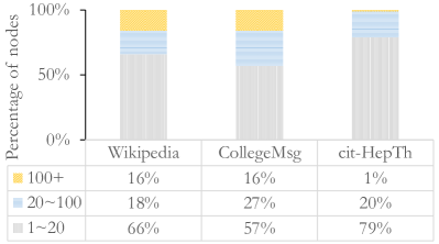
Figure 3: Distribution of Node Degree.

IV-D Link Prediction Results

In this part, we compare S2T with multiple competitors on the link prediction task and divide the dataset into a training set and a test set in chronological order of 80% and 20%. After split the dataset, we first train model on the training set and then conduct link predictions on the test set. In the test set, for each interaction, we define it as positive pair and random sample a negative pair (i.e., two nodes have never interacted with each other). After an equal number of positive and negative sample pairs are generated, we use a logistic regression function to determine the positives and negatives of each pair and compare them with the true results. We leverage the Accuracy (ACC) and F1-Score (F1) as performance metrics. As shown in Table III, the proposed S2T achieves the best performances compared with various existing baselines on all three datasets.

In these three datasets, S2T obtains the best improvement on cit-HepTh and the least improvement on CollegeMsg. We argue that this phenomenon is related to the distribution of node degrees on different datasets. Thus we provide pie charts of degree distributions to explain this problem. In Figure 3, the number of nodes with different degrees is given. We simply define nodes with a degree between $1$ and $20$ as low-active nodes (i.e., long-tail nodes) and nodes with a degree above $100$ as high-active nodes, then can find that the number of low-active nodes accounts for a higher percentage than the sum of the other two categories. This is in line with the phenomenon we pointed out above that long-tail nodes are the most common category of nodes in the graph.

Here we give the number of the long-tail nodes on three datasets: Wikipedia (5045, 65.69%), CollegeMsg (1082, 56.97%), and cit-HepTh (5999, 79.17%). Moreover, in conjunction with Table III, if a dataset has a larger proportion of long-tailed nodes, the more our global module works, and thus the better S2T improves on that dataset. The experimental results and data analysis nicely corroborates the effectiveness of our proposed global module for information enhancement of long-tail nodes.

As mentioned above, the baseline methods include two parts: static methods and temporal methods. According to the link prediction result, most of the temporal methods achieve better performance than static methods, which means that the temporal information in node interactions is important. Compared to HTNE, which models temporal information with the Hawkes process, and TREND, which models structural information with GNN, our method S2T achieves better performance by combining both temporal and structural information. This indicates that the alignment loss can constrain S2T to capture the two different types of information effectively.

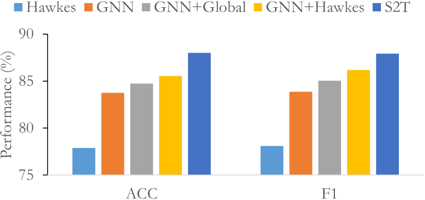
(a) Wikipedia

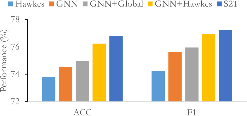
(b) CollegeMsg

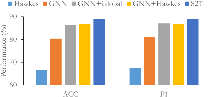
(c) cit-HepTh

Figure 4: Ablation Study on Three Datasets.

IV-E Ablation Study

Note that in the proposed S2T, we introduce the temporal information modeling module based on the Hawkes process and the structural information modeling module. The structural module contains a local module based on GNN and a global module. In this part, we will discuss different modules’ effects on performance.

More specially, we select five module combinations: (1) only temporal information modeling (i.e., Hawkes module); (2) only local structural information modeling (i.e., GNN module); (3) both local and global structural information modeling (i.e., GNN+Global); (4) align temporal information with local structural information (i.e., GNN+Hawkes); (5) the final model (i.e., S2T).

As shown in Figure 4, we can find that both Hawkes and GNN modules can only achieve sub-optimal performance. If the two modules are combined, the performance of the GNN+Hawkes module is significantly improved, which demonstrates the effect of the proposed alignment loss.

Furthermore, when the GNN module incorporates global information, the performance of the GNN+Global module is also further improved. By comparing module GNN and GNN+Global, the average magnitude of improvement on three different datasets is 0.49% on CollegeMsg, 1.28% on Wikipedia, and 7.40% on cit-HepTh, which is consistent with the ranking of the long-tailed node proportion in Figure 3. It means that the datasets with more long-tail nodes have a larger performance improvement, which proves that our proposed global module is effective in enhancing long-tail nodes.

IV-F Parameter Sensitivity Analysis

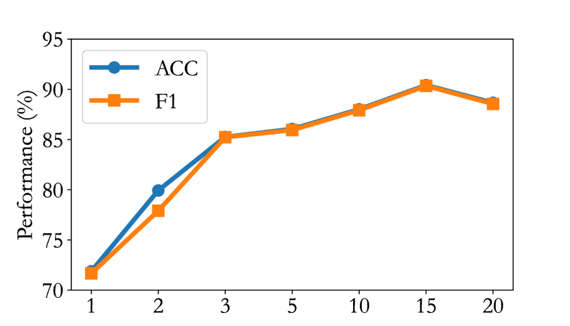
(a) Wikipedia

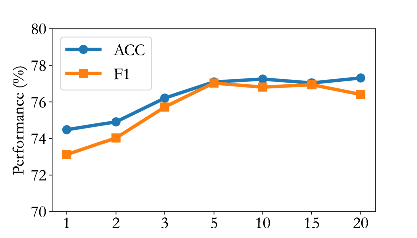
(b) CollegeMsg

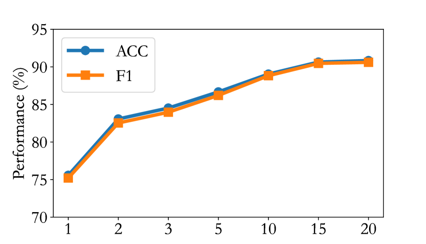
(c) cit-HepTh

Figure 5: Parameter Sensitivity of Historical Sequence Length.

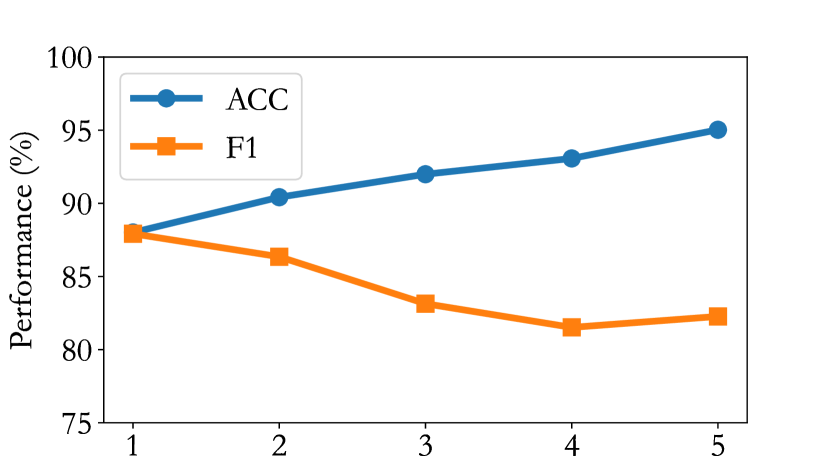
(a) Wikipedia

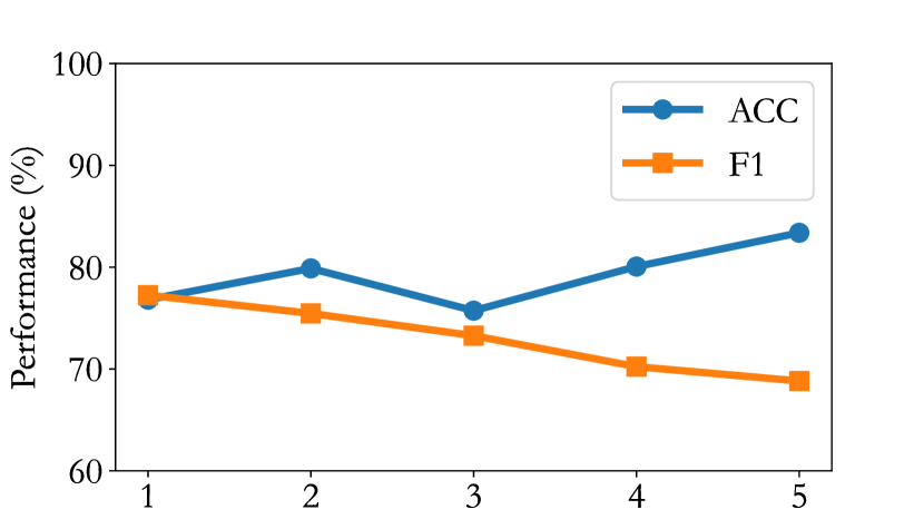
(b) CollegeMsg

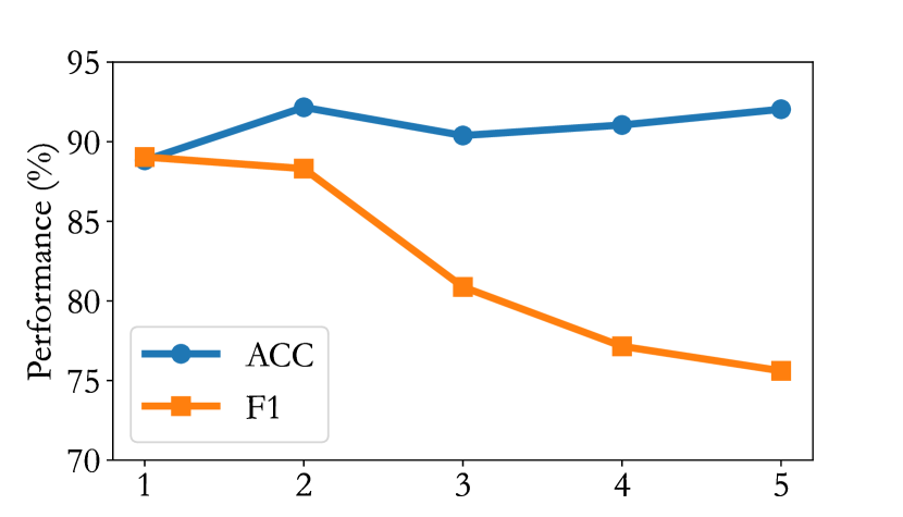
(c) cit-HepTh

Figure 6: Parameter Sensitivity of Negative Sample Number.

IV-F1 Length of Historical Neighbor Sequence

In a temporal graph, node neighbors are fed into the model in batches in the form of interaction sequences. But in actual training, if we obtain all of its neighbors for each node, the computational pattern of each batch can not be fixed, which brings great computational inconvenience. To maintain the convenient calculation of batch training, it is hard for the model to obtain multiple neighbor sequences with different lengths.

According to Figure 3, most nodes have few neighbors, especially in the first half of the time zone. Referencing previous works [37, 42, 43, 41, 39], many temporal graph methods choose to fix the sequence length $S$ of neighbor sequence and obtain each node’s latest $S$ neighbors instead of saving full neighbors. If a node doesn’t have enough neighbors at a certain timestamp, we mask the empty positions. Thus we need to discuss a question, how do different values of $S$ influence performance?

As shown in Figure 5, with the change of $S$, the model performance can achieve better results when $S$ is taken as $10/15/20$. In particular, the optimal value of $S$ is taken differently on different datasets. On Wikipedia and cit-HepTh datasets, the optimal value of $S$ are $15$ and $20$, respectively. But on the CollegeMsg dataset, when we select $S$ as $20$, the ACC performance and F1 performance show a large deviation. In contrast, the two performance appear more balanced when $S$ is taken to be $10$ or $15$. For this phenomenon, we argue that with the continuous increase of $S$ ($0-15$), the model can capture more and more neighbor information. But after that, when $S$ continues to increase, too many unnecessary neighbor nodes will be added. These neighbors usually interact earlier, thus the information contained in their interaction can hardly be used as an effective reference for future prediction.

In addition, too many neighbors will increase the amount of computation. Therefore, in the real training, although the performance is better when $S$ is $15$, we default $S$ to $10$ as the hyper-parameter value for the convenience of calculation.

IV-F2 Negative Sample Number

The negative sample number $Q$ is a hyper-parameter utilized to control how many negative pairs are generated to the link prediction task loss in Eq. (11). As shown in Figure 6, we can find that with the increase of the negative sample numbers, although the ACC performance increases, the F1 score decreases. It means that an increase in the number of negative samples will lead to an imbalance in the proportion of positive and negative samples in the test, resulting in the above phenomenon. Thus on all datasets, it is robust to select one negative sample pair to benchmark one positive sample pair.

IV-G Convergence of Loss

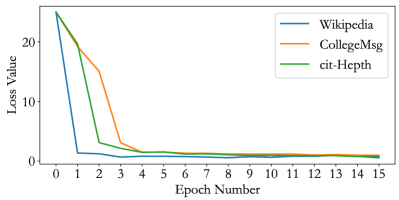
Figure 7: Convergence of Loss.

As shown in Figure 7, in all three datasets, the loss values of S2T can achieve convergence after a few epochs. By comparing the convergence rules of the three datasets, we find that the data set with more nodes has a faster convergence speed of the corresponding loss value. It means that more node samples are provided in each training so that the model can learn better.

Combined with the above discussion, S2T has time complexity of $O(t|E|d^{3})$ and can converge quickly with a small amount of epoch training, which means that S2T can be more adaptable to large-scale data.

V Conclusion

We propose a self-supervised graph learning method S2T, by extracting both temporal and structural information to learn more informative node representations. The alignment loss is introduced to narrow the gap between temporal and structural intensities, which can encourage the model to learn both valid temporal and structural information.. We also construct a global module to enhance the long-tail nodes’ information. Experiments on several datasets prove the proposed S2T achieves the best performance in all baseline methods.

In the future, we will try to construct a more general framework to combine multi-modal information. With the rapid development of various fields of deep learning, how to propose a unified framework to deal with data from different sources has become a hot issue that researchers pay attention to. Graph learning can model the potential relationships between these data well, so a general framework based on graph learning may bring better inspiration for multi-modal information fusion.

References

- [1] P. Cui, X. Wang, J. Pei, and W. Zhu, “A survey on network embedding,” IEEE transactions on knowledge and data engineering, vol. 31, no. 5, pp. 833–852, 2018.
- [2] Z. Wu, S. Pan, F. Chen, G. Long, C. Zhang, and S. Y. Philip, “A comprehensive survey on graph neural networks,” IEEE transactions on neural networks and learning systems, vol. 32, no. 1, pp. 4–24, 2020.
- [3] J. Qiu, Y. Dong, H. Ma, J. Li, K. Wang, and J. Tang, “Network embedding as matrix factorization: Unifying deepwalk, line, pte, and node2vec,” in Proceedings of the eleventh ACM international conference on web search and data mining, 2018, pp. 459–467.
- [4] X. Wang, X. He, M. Wang, F. Feng, and T.-S. Chua, “Neural graph collaborative filtering,” in Proceedings of the 42nd international ACM SIGIR conference on Research and development in Information Retrieval, 2019, pp. 165–174.
- [5] S. Pan, R. Hu, S.-f. Fung, G. Long, J. Jiang, and C. Zhang, “Learning graph embedding with adversarial training methods,” IEEE transactions on cybernetics, vol. 50, no. 6, pp. 2475–2487, 2019.
- [6] L. Li, S. Wang, X. Liu, E. Zhu, L. Shen, K. Li, and K. Li, “Local sample-weighted multiple kernel clustering with consensus discriminative graph,” IEEE Transactions on Neural Networks and Learning Systems, pp. 1–14, 2022.
- [7] M. Ou, P. Cui, J. Pei, Z. Zhang, and W. Zhu, “Asymmetric transitivity preserving graph embedding,” in Proceedings of the 22nd ACM SIGKDD international conference on Knowledge discovery and data mining, 2016, pp. 1105–1114.
- [8] Z. Li, H. Liu, Z. Zhang, T. Liu, and N. N. Xiong, “Learning knowledge graph embedding with heterogeneous relation attention networks,” IEEE Transactions on Neural Networks and Learning Systems, vol. 33, no. 8, pp. 3961–3973, 2021.
- [9] Z. Kang, Z. Lin, X. Zhu, and W. Xu, “Structured graph learning for scalable subspace clustering: From single view to multiview,” IEEE Transactions on Cybernetics, vol. 52, no. 9, pp. 8976–8986, 2021.
- [10] Z. Kang, H. Pan, S. C. Hoi, and Z. Xu, “Robust graph learning from noisy data,” IEEE transactions on cybernetics, vol. 50, no. 5, pp. 1833–1843, 2019.
- [11] S. Zhang, H. Chen, X. Ming, L. Cui, H. Yin, and G. Xu, “Where are we in embedding spaces?” in Proceedings of the 27th ACM SIGKDD Conference on Knowledge Discovery and Data Mining, 2021, pp. 2223–2231.
- [12] D. Bo, X. Wang, C. Shi, M. Zhu, E. Lu, and P. Cui, “Structural deep clustering network,” in Proceedings of the web conference 2020, 2020, pp. 1400–1410.
- [13] C. Huang, Q. Zhang, D. Guo, X. Zhao, and X. Wang, “Discovering association rules with graph patterns in temporal networks,” Tsinghua Science and Technology, vol. 28, no. 2, pp. 344–359, 2022.
- [14] A. G. Hawkes, “Point spectra of some mutually exciting point processes,” Journal of the Royal Statistical Society: Series B (Methodological), vol. 33, no. 3, pp. 438–443, 1971.
- [15] M. Mao, J. Lu, G. Zhang, and J. Zhang, “Multirelational social recommendations via multigraph ranking,” IEEE transactions on cybernetics, vol. 47, no. 12, pp. 4049–4061, 2016.
- [16] B. Wu, X. He, Q. Zhang, M. Wang, and Y. Ye, “Gcrec: Graph-augmented capsule network for next-item recommendation,” IEEE Transactions on Neural Networks and Learning Systems, 2022.
- [17] L. Bai, L. Rossi, L. Cui, J. Cheng, and E. R. Hancock, “A quantum-inspired similarity measure for the analysis of complete weighted graphs,” IEEE transactions on cybernetics, vol. 50, no. 3, pp. 1264–1277, 2019.
- [18] D. Hu, K. Liang, S. Zhou, W. Tu, M. Liu, and X. Liu, “scdfc: A deep fusion clustering method for single-cell rna-seq data,” Briefings in Bioinformatics, p. bbad216, 2023.
- [19] S. Ji, S. Pan, E. Cambria, P. Marttinen, and S. Y. Philip, “A survey on knowledge graphs: Representation, acquisition, and applications,” IEEE transactions on neural networks and learning systems, vol. 33, no. 2, pp. 494–514, 2021.
- [20] K. Liang, L. Meng, M. Liu, Y. Liu, W. Tu, S. Wang, S. Zhou, X. Liu, and F. Sun, “Reasoning over different types of knowledge graphs: Static, temporal and multi-modal,” arXiv preprint arXiv:2212.05767, 2022.
- [21] J. Sun, W. Zheng, Q. Zhang, and Z. Xu, “Graph neural network encoding for community detection in attribute networks,” IEEE Transactions on Cybernetics, vol. 52, no. 8, pp. 7791–7804, 2021.
- [22] M. Liu, Y. Liu, K. Liang, S. Wang, S. Zhou, and X. Liu, “Deep temporal graph clustering,” arXiv preprint arXiv:2305.10738, 2023.
- [23] Y. Fang, X. Zhao, P. Huang, W. Xiao, and M. de Rijke, “Scalable representation learning for dynamic heterogeneous information networks via metagraphs,” ACM Transactions on Information Systems (TOIS), vol. 40, no. 4, pp. 1–27, 2022.
- [24] M. Liu, J. Wu, and Y. Liu, “Embedding global and local influences for dynamic graphs,” in Proceedings of the 31st ACM International Conference on Information and Knowledge Management, 2022, pp. 4249–4253.
- [25] J. Gan, R. Hu, Y. Mo, Z. Kang, L. Peng, Y. Zhu, and X. Zhu, “Multigraph fusion for dynamic graph convolutional network,” IEEE Transactions on Neural Networks and Learning Systems, 2022.
- [26] Z. Song, X. Yang, Z. Xu, and I. King, “Graph-based semi-supervised learning: A comprehensive review,” IEEE Transactions on Neural Networks and Learning Systems, 2022.
- [27] S. Lin, C. Liu, P. Zhou, Z.-Y. Hu, S. Wang, R. Zhao, Y. Zheng, L. Lin, E. Xing, and X. Liang, “Prototypical graph contrastive learning,” IEEE Transactions on Neural Networks and Learning Systems, 2022.
- [28] B. Perozzi, R. Al-Rfou, and S. Skiena, “Deepwalk: Online learning of social representations,” in Proceedings of the 20th ACM SIGKDD international conference on Knowledge discovery and data mining, 2014, pp. 701–710.
- [29] A. Grover and J. Leskovec, “node2vec: Scalable feature learning for networks,” in Proceedings of the 22nd ACM SIGKDD international conference on Knowledge discovery and data mining, 2016, pp. 855–864.
- [30] T. N. Kipf and M. Welling, “Variational graph auto-encoders,” in NeurIPS, 2016.
- [31] W. Hamilton, Z. Ying, and J. Leskovec, “Inductive representation learning on large graphs,” Advances in neural information processing systems, vol. 30, 2017.
- [32] C. Gao, J. Zhu, F. Zhang, Z. Wang, and X. Li, “A novel representation learning for dynamic graphs based on graph convolutional networks,” IEEE Transactions on Cybernetics, 2022.
- [33] Z. Cui, Z. Li, S. Wu, X. Zhang, Q. Liu, L. Wang, and M. Ai, “Dygcn: Efficient dynamic graph embedding with graph convolutional network,” IEEE Transactions on Neural Networks and Learning Systems, 2022.
- [34] A. Pareja, G. Domeniconi, J. Chen, T. Ma, T. Suzumura, H. Kanezashi, T. Kaler, T. Schardl, and C. Leiserson, “Evolvegcn: Evolving graph convolutional networks for dynamic graphs,” in Proceedings of the AAAI conference on artificial intelligence, vol. 34, no. 04, 2020, pp. 5363–5370.
- [35] A. Sankar, Y. Wu, L. Gou, W. Zhang, and H. Yang, “Dysat: Deep neural representation learning on dynamic graphs via self-attention networks,” in Proceedings of the 13th international conference on web search and data mining, 2020, pp. 519–527.
- [36] G. H. Nguyen, J. B. Lee, R. A. Rossi, N. K. Ahmed, E. Koh, and S. Kim, “Continuous-time dynamic network embeddings,” in Companion proceedings of the the web conference 2018, 2018, pp. 969–976.
- [37] Y. Zuo, G. Liu, H. Lin, J. Guo, X. Hu, and J. Wu, “Embedding temporal network via neighborhood formation,” in Proceedings of the 24th ACM SIGKDD international conference on knowledge discovery and data mining, 2018, pp. 2857–2866.
- [38] Y. Lu, X. Wang, C. Shi, P. S. Yu, and Y. Ye, “Temporal network embedding with micro-and macro-dynamics,” in Proceedings of the 28th ACM international conference on information and knowledge management, 2019, pp. 469–478.
- [39] D. Xu, C. Ruan, E. Korpeoglu, S. Kumar, and K. Achan, “Inductive representation learning on temporal graphs,” in ICLR, 2020.
- [40] M. Liu and Y. Liu, “Inductive representation learning in temporal networks via mining neighborhood and community influences,” in Proceedings of the 44th International ACM SIGIR Conference on Research and Development in Information Retrieval, 2021, pp. 2202–2206.
- [41] Z. Wen and Y. Fang, “Trend: Temporal event and node dynamics for graph representation learning,” in Proceedings of the ACM Web Conference 2022, 2022, pp. 1159–1169.
- [42] L. Hu, C. Li, C. Shi, C. Yang, and C. Shao, “Graph neural news recommendation with long-term and short-term interest modeling,” Information Processing and Management, vol. 57, no. 2, p. 102142, 2020.
- [43] M. Liu, Z.-W. Quan, J.-M. Wu, Y. Liu, and M. Han, “Embedding temporal networks inductively via mining neighborhood and community influences,” Applied Intelligence, pp. 1–20, 2022.
- [44] M. Granovetter, “Threshold models of collective behavior,” American journal of sociology, vol. 83, no. 6, pp. 1420–1443, 1978.
- [45] Y. Li, J. Fan, Y. Wang, and K.-L. Tan, “Influence maximization on social graphs: A survey,” IEEE Transactions on Knowledge and Data Engineering, vol. 30, no. 10, pp. 1852–1872, 2018.
- [46] J.-T. Tian, Y.-T. Wang, and X.-J. Feng, “A new hybrid algorithm for influence maximization in social networks,” Jisuanji Xuebao(Chinese Journal of Computers), vol. 34, no. 10, pp. 1956–1965, 2011.
- [47] E. Perez, F. Strub, H. De Vries, V. Dumoulin, and A. Courville, “Film: Visual reasoning with a general conditioning layer,” in Proceedings of the AAAI Conference on Artificial Intelligence, vol. 32, no. 1, 2018.
- [48] H. Chen, H. Yin, W. Wang, H. Wang, Q. V. H. Nguyen, and X. Li, “Pme: projected metric embedding on heterogeneous networks for link prediction,” in Proceedings of the 24th ACM SIGKDD international conference on knowledge discovery and data mining, 2018, pp. 1177–1186.
- [49] T. Mikolov, I. Sutskever, K. Chen, G. S. Corrado, and J. Dean, “Distributed representations of words and phrases and their compositionality,” Advances in neural information processing systems, vol. 26, 2013.
- [50] S. Kumar, X. Zhang, and J. Leskovec, “Predicting dynamic embedding trajectory in temporal interaction networks,” in Proceedings of the 25th ACM SIGKDD international conference on knowledge discovery and data mining, 2019, pp. 1269–1278.
- [51] P. Panzarasa, T. Opsahl, and K. M. Carley, “Patterns and dynamics of users’ behavior and interaction: Network analysis of an online community,” Journal of the American Society for Information Science and Technology, vol. 60, no. 5, pp. 911–932, 2009.
- [52] J. Leskovec, J. Kleinberg, and C. Faloutsos, “Graphs over time: densification laws, shrinking diameters and possible explanations,” in Proceedings of the eleventh ACM SIGKDD international conference on Knowledge discovery in data mining, 2005, pp. 177–187.
- [53] D. P. Kingma and J. Ba, “Adam: A method for stochastic optimization,” in ICLR, 2014.