Bridging the Usability Gap: Theoretical and Methodological Advances for Spectral Learning of Hidden Markov Models

Abstract

The Baum-Welch (B-W) algorithm is the most widely accepted method for inferring hidden Markov models (HMM). However, it is prone to getting stuck in local optima, and can be too slow for many real-time applications. Spectral learning of HMMs (SHMM), based on the method of moments (MOM) has been proposed in the literature to overcome these obstacles. Despite its promises, asymptotic theory for SHMM has been elusive, and the long-run performance of SHMM can degrade due to unchecked propagation of error. In this paper, we (1) provide an asymptotic distribution for the approximate error of the likelihood estimated by SHMM, (2) propose a novel algorithm called projected SHMM (PSHMM) that mitigates the problem of error propagation, and (3) develop online learning variants of both SHMM and PSHMM that accommodate potential nonstationarity. We compare the performance of SHMM with PSHMM and estimation through the B-W algorithm on both simulated data and data from real world applications, and find that PSHMM not only retains the computational advantages of SHMM, but also provides more robust estimation and forecasting.

Keywords: hidden Markov models (HMM), spectral estimation, projection-onto-simplex, online learning, time series forecasting

1 Introduction

The hidden Markov model (HMM) (Baum and Petrie,, 1966) is a widespread model with applications in many areas, such as finance, natural language processing and biology. An HMM is a stochastic probabilistic model for sequential or time series data that assumes that the underlying dynamics of the data are governed by a Markov chain. (Knoll et al.,, 2016).

The Baum-Welch algorithm (Baum et al.,, 1970), which is a special case of the expectation–maximization (E-M) algorithm (Dempster et al.,, 1977) based on maximum likelihood estimation (MLE), is a popular approach for inferring the parameters of the HMM. However, the E-M algorithm can require a large number of iterations until the parameter estimates converge–which has a large computational cost, especially for large-scale time series data–and can easily get trapped in local optima. In order to overcome these issues especially for large, high dimensional time series, Hsu et al., (2012) proposed a spectral learning algorithm for HMMs (SHMM), based on the method of moments (MOM), with attractive theoretical properties. However, the asymptotic error distribution of the algorithm was not well-characterized. Later, Rodu, (2014) improved the spectral estimation algorithm and extended it to HMMs with high-dimensional and continuously-distributed output, but again did not address the asymptotic error distribution. In this manuscript, we provide a theoretical discussion of the asymptotic error behavior of SHMM algorithms.

In addition to investigating the asymptotic error distribution, we provide a novel improvement to the SHMM family of algorithms. Our improvement is motivated from an extensive simulation study of the methods proposed in Hsu et al., (2012) and Rodu, (2014). We found that spectral estimation does not provide stable results under the low signal-noise ratio setting. We propose a new spectral estimation method, the projected SHMM (PSHMM), that leverages a novel regularization technique that we call ‘projection-onto-simplex’ regularization. The PSHMM largely retains the computational advantages of SHMM methods without sacrificing accuracy.

Finally, we provide a novel extension of spectral estimation (including all SHMM and PSHMM approaches) to allow for online learning. We propose two approaches – the first speeds up computational time required for learning a model in large data settings, and the second incorporates “forgetfulness” which allows for adapting to changing dynamics of the data. This speed and flexibility is crucial, for instance, in high frequency trading, and we show the effectiveness of the PSHMM on real data in this setting.

The structure of this paper is as follows: In the rest of this section, we will introduce existing models. In Section 2, we provide theorems for the asymptotic properties of SHMMs. Section 3 introduces our new method, PSHMM. In Section 4, we extend the spectral estimation to online learning for both SHMM and PSHMM. Then, section 5 shows the simulation results and Section 6 shows the application on high frequency trading. We provide extensive discussion in Section 7.

1.1 The hidden Markov model

The standard HMM (Baum and Petrie,, 1966) is defined by a set of $S$ hidden categorical states $1,2,\cdots,S$ that evolve according to a Markov chain. We denote the hidden state at time $t$ as $h_{t}$. The Markov chain is characterized by an initial probability $\pi_{0}=[\pi_{0}^{(1)},\cdots,\pi_{0}^{(S)}]$ where $h_{1}\sim Multinomial(\pi_{0}^{(1)},\cdots,\pi_{0}^{(S)})$ , and a transition matrix $\mathbf{T}=[\mathbf{T}_{ij}]_{i=1,\cdots,S}^{j=1,\cdots,S}$ where $\mathbf{T}_{ij}=\mathrm{P}(h_{t+1}=j|h_{t}=i)$ for $\forall t$. The emitted observation $X_{t}$ is distributed conditional on the value of the hidden state at time $t$, $X_{t}|h_{t}=s\sim\mathcal{F}_{s}$ where $\mathcal{F}_{s}$ is the emission distribution conditioned on the hidden state $h_{t}=s$. The standard HMM’s parameters are $\left(\pi_{0},\mathbf{T},\{\mathcal{F}_{s}\}_{s=1}^{S}\right)$. Figure 1 is a graphical representation of the standard HMM. Typically, if the emission follows a Gaussian distribution, then we call it Gaussian HMM (GHMM).

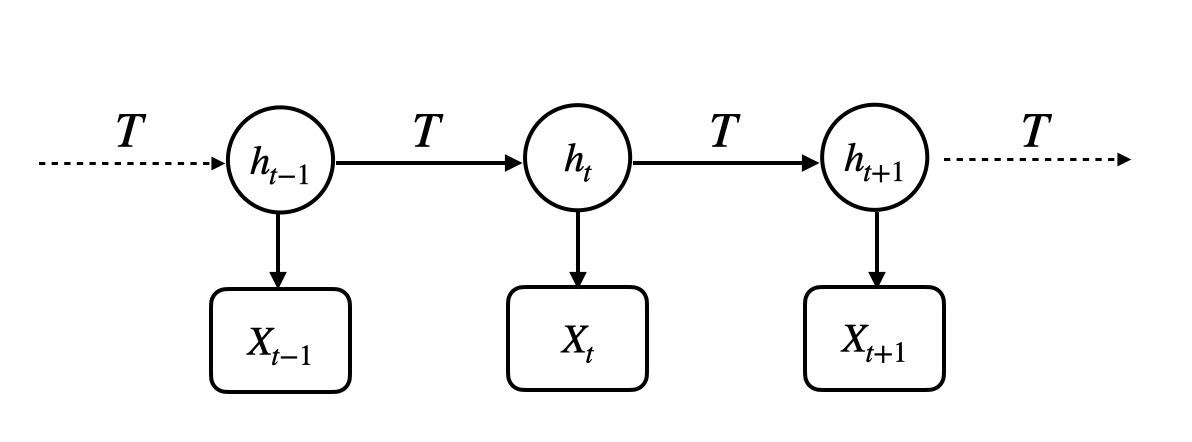
Figure 1: Model structure of standard HMM. $\{h_{t}\}$ is a latent Markov chain that evolves according to transition matrix $\mathbf{T}$. For each time stamp $t$, the observed $X_{t}$ is generated according to the emission distribution associated with $h_{t}$.

1.2 Spectral learning of HMM

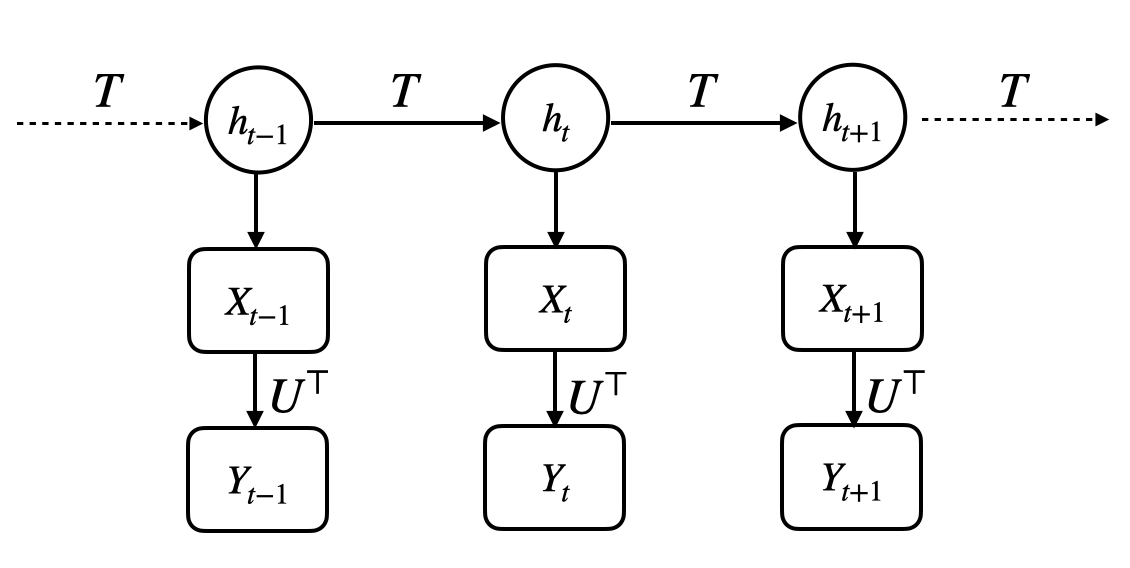
Figure 2: Spectral estimation model by Rodu, (2014). In addition to containing the latent state series $\{h_{t}\}_{t}$ and observed series $\{X_{t}\}_{t}$, Rodu, (2014) introduced a reduced-dimensional series $\{Y_{t}=U^{\top}X_{t}\}$ which is a projection of $X_{t}$ on a lower-dimensional subspace whose dimensionality is equal to the number of hidden states. Spectral estimation proceeds based on $\{Y_{t}\}_{t}$.

The model proposed by Rodu, (2014) is shown in Figure 2. Again, $h_{t}$ denotes the hidden state at time $t$, and $X_{t}$ the emitted observation. For estimation of the model, these observations are further projected onto a lower dimensional space of dimensionality $d$ and the lower dimensional observations are denoted $y_{t}=U^{\top}x_{t}$. We discuss the choice of dimension $d$ and the projection of the observations in Section 3.3.

Using the spectral estimation framework, the likelihood can be written as:

$$Pr(x_{1:t}) = c_{\infty}^{\top}C(y_{t})C(y_{t-1})\cdots C(y_{1})c_{1},$$ (1)

where

$$c_{1}=\mu,c_{\infty}^{\top}=\mu^{\top}\Sigma^{-1},C(y)=K(y)\Sigma^{-1},$$

$$\mu=E(y_{1})=U^{\top}M\pi,$$

$$\Sigma=E(y_{2}y_{1}^{\top})=U^{\top}MTdiag(\pi)M^{\top}U,$$

$$K(a)=\mathrm{E}(y_{3}y_{1}^{\top}y_{2}^{\top})a=U^{\top}MTdiag(M^{\top}Ua)Tdiag(\pi)(M^{\top}U),$$

$$M=[M_{1},\cdots,M_{S}]\text{ where }M_{i}=\mathrm{E}(X|i).$$

These quantities can be empirically estimated as:

$$\widehat{P}r(x_{1:t}) = \hat{c}_{\infty}^{\top}\hat{C}(y_{t})\hat{C}(y_{t-1})\cdots\hat{C}(y_{1})\hat{c}_{1},$$ (2)

where

$$\hat{c}_{1}=\hat{\mu},\hat{c}_{\infty}^{\top}=\hat{\mu}^{\top}\hat{\Sigma}^{-1},\hat{C}(y)=\hat{K}(y)\hat{\Sigma}^{-1},$$

$$\hat{\mu}=\frac{1}{N}\sum_{i=1}^{N}Y_{i},$$

$$\hat{\Sigma}=\frac{1}{N}\sum_{i=1}^{N-1}Y_{i+1}Y_{i}^{\top},$$

$$\hat{K}(y)=\frac{1}{N}\sum_{i=1}^{N-2}Y_{i+2}Y_{i}^{\top}\cdot Y_{i+1}^{\top}y.$$

Prediction of $y_{t}$ is computed recursively by:

$$\hat{y}_{t} = \frac{C(y_{t-1})\hat{y}_{t-1}}{c^{\top}_{\infty}C(y_{t-1})\hat{y}_{t-1}};$$ (3)

Observation $x_{t}$ can be recovered as:

$$\hat{x_{t}}|x_{1},x_{2},\cdots,x_{t-1}=U\hat{y_{t}}.$$ (4)

In the above exposition of spectral likelihood estimation, moment estimation, and recursive forecasting we assume a discrete output HMM. For a continuous output HMM, the spectral estimation of likelihood is slightly different. We need some kernel function $G(x)$ to calculate $K$, so $K(a)=U^{\top}MTdiag(M^{\top}UG(a))Tdiag(\pi)(M^{\top}U)$ (for more on $G(\cdot)$ see Rodu,, 2014). In this paper, we will use a linear kernel $G(a)=a$ for simplicity. In this case, the moment estimation and recursive forecasting for the continuous case are identical to the discrete case. See Rodu et al., (2013) for detailed derivations and mathematical proofs of these results.

2 Theoretical Properties of SHMM

In general, SHMM estimates the likelihood through the MOM. Although MOM gives fast approximation, the theoretical properties of SHMM estimation are less well studied. Hsu et al., (2012) and Rodu et al., (2013) give the conditions where the spectral estimator converges to the true likelihood almost surely:

$$\widehat{P}r(x_{1:T}) = \hat{c}_{\infty}^{\top}\hat{C}(y_{t})\hat{C}(y_{t-1})\cdots\hat{C}(y_{1})\hat{c}_{1}\xrightarrow[]{a.s.}Pr(x_{1:T}),$$ (5)

In this manuscript, we study the asymptotic distribution of $\hat{P}r(x_{1:T})-Pr(x_{1:T})$. Theorem 1 shows a CLT type bound of the approximation error.

First, however, we identify the sources of error for the SHMM in Lemma 1.

Lemma 1 makes use of the what we refer to as the ‘$\Delta$’ terms, defined through the following equations: $\widehat{\mu}=\mu+\widehat{\Delta\mu}$, $\widehat{\Sigma}=\Sigma+\widehat{\Delta\Sigma}$, $\widehat{K}=K+\widehat{\Delta K}$.

Lemma 1.

$$\widehat{P}r(x_{1:T}) = Pr(x_{1:T})+(v+\tilde{v})^{\top}\widehat{\Delta\mu}+\sum_{t=1}^{T}a_{t}^{\top}\widehat{\Delta K}(y_{t})\tilde{a_{t}}-\sum_{t=0}^{T}b_{t}^{\top}\widehat{\Delta\Sigma}\tilde{b_{t}}+\mathcal{O}_{p}(N^{-1}),$$

where

$$v=\left(\mu^{\top}\Sigma^{-1}K(y_{T})\cdots K(y_{1})\Sigma^{-1}\right)^{\top}; \quad\tilde{v}=\Sigma^{-1}K(y_{T})\cdots K(y_{1})\Sigma^{-1}\mu;$$

$$a_{t}=\left(\mu^{\top}\Sigma^{-1}K(y_{T})\Sigma^{-1}\cdots K(y_{t+1})\Sigma^{-1}\right)^{\top}; \quad\tilde{a_{t}}=\Sigma^{-1}K(y_{t-1})\cdots K(y_{1})\Sigma^{-1}\mu;$$

$$b_{t}=\left(\mu^{\top}\Sigma^{-1}K(y_{T})\Sigma^{-1}\cdots\Sigma^{-1}K(y_{t+1})\Sigma^{-1}\right)^{\top}; \quad\tilde{b_{t}}=\Sigma^{-1}K(y_{t})\Sigma^{-1}\cdots K(y_{1})\Sigma^{-1}\mu.$$

We provide a detailed proof of this lemma in the supplementary material. The basic strategy is to fully expand $\widehat{P}r(x_{1:T})-Pr(x_{1:T})$ after rewriting the estimated quantities as a sum of the true quantity plus an error term. We then categorize each summand based on how many ‘$\Delta$’ terms it has. There are three categories: terms with zero ‘$\Delta$’ terms (i.e. the true likelihood $Pr(x_{1:T})$), terms with only one ‘$\Delta$’ (i.e. $(v+\tilde{v})^{\top}\widehat{\Delta\mu}+\sum_{t=1}^{T}a_{t}^{\top}\widehat{\Delta K}(y_{t})\tilde{a_{t}}-\sum_{t=0}^{T}b_{t}^{\top}\widehat{\Delta\Sigma}\tilde{b_{t}}$), and all remaining terms, which involve at least two ‘$\Delta$’ quantities, and can be relegated to $\mathcal{O}_{p}(N^{-1})$.

Lemma 1 shows how the estimated error propagates to the likelihood approximation. We can leverage the fact that our moment estimators have a central limit theorem (CLT) property to obtain the desired results in Theroem 1.

We denote the outer product as $\otimes$, and define a “flattening” operator $\mathcal{F}(\cdot)$ for both matrices and 3-way tensors. For matrix $A_{d\times d}$,

$$\mathcal{F}(A)=[A^{(1,1)},A^{(1,2)},\cdots,A^{(d,d)}]^{\top};$$

For tensor $B_{d\times d\times d}$,

$$\mathcal{F}(B)=[B^{(1,1,1)},B^{(1,1,2)},\cdots,B^{(1,1,d)},B^{(1,2,1)},B^{(1,2,2)},\cdots,B^{(1,2,d)},\cdots,B^{(1,d,d)},\cdots,B^{(d,d,d)}]^{\top}$$

We now state and prove our main theorem.

Theorem 1.

$$\sqrt{N}(\widehat{P}r(x_{1:T})-Pr(x_{1:T})) \xrightarrow[]{d} N\left(0,\beta^{\top}Cov\left(\begin{bmatrix}Y_{1}\\ \mathcal{F}(Y_{2}\otimes Y_{1})\\ \mathcal{F}(Y_{3}\otimes Y_{1}\otimes Y_{2})\end{bmatrix}\right)\beta\right),$$

where

$$\beta=\left[(v+\tilde{v})^{\top};-\left(\sum_{t=0}^{T}\mathcal{F}(b_{t}\otimes\tilde{b}_{t})\right)^{\top};\left(\sum_{t=1}^{T}\mathcal{F}(a_{t}\otimes\tilde{a}_{t}\otimes y_{t})\right)^{\top}\right]^{\top}$$

and $v,\tilde{v},a_{t},\tilde{a}_{t},b_{t},\tilde{b}_{t}$ are defined as in Lemma 1.

Proof (Theorem 1).

We flatten $\widehat{\Delta\Sigma}$ and $\widehat{\Delta K}$ as

$$\mathcal{F}(\widehat{\Delta\Sigma}) = [\widehat{\Delta\Sigma}^{(1,1)},\widehat{\Delta\Sigma}^{(1,2)},\cdots,\widehat{\Delta\Sigma}^{(d,d)}]^{\top},$$

$$\mathcal{F}(\widehat{\Delta K}) = [\widehat{\Delta K}^{(1,1,1)},\widehat{\Delta K}^{(1,1,2)},\cdots,\widehat{\Delta K}^{(d,d,d)}]^{\top}.$$

Rewriting $a_{t}^{\top}\widehat{\Delta K}(y_{t})\tilde{a_{t}}$ and $b_{t}^{\top}\widehat{\Delta\Sigma}\tilde{b_{t}}$ in Eq 1 as

$$a_{t}^{\top}\widehat{\Delta K}(y_{t})\tilde{a_{t}} = \mathcal{F}(a_{t}\otimes\tilde{a}_{t}\otimes y_{t})^{\top}\cdot\mathcal{F}(\widehat{\Delta K}),$$

$$b_{t}^{\top}\widehat{\Delta\Sigma}\tilde{b_{t}} = \mathcal{F}(b_{t}\otimes\tilde{b}_{t})^{\top}\cdot\mathcal{F}(\widehat{\Delta\Sigma}),$$

we have

$$\widehat{P}r(x_{1:T})-Pr(x_{1:T})-O_{p}(N^{-1})$$

$$= \left[(v+\tilde{v})^{\top};-\left(\sum_{t=0}^{T}\mathcal{F}(b_{t}\otimes\tilde{b}_{t})\right)^{\top};\left(\sum_{t=1}^{T}\mathcal{F}(a_{t}\otimes\tilde{a}_{t}\otimes y_{t})\right)^{\top}\right]\cdot\begin{bmatrix}\widehat{\Delta\mu}\\ \mathcal{F}(\widehat{\Delta\Sigma})\\ \mathcal{F}(\widehat{\Delta K})\end{bmatrix}$$

$$= \beta^{\top}\cdot\widehat{\Delta\theta}.$$

Since the CLT applies seperately to $\widehat{\Delta\mu},\widehat{\Delta\Sigma},\widehat{\Delta K}$, then

$$\sqrt{N}\widehat{\Delta\theta} = \sqrt{N}\begin{bmatrix}\frac{1}{N}\sum_{i=1}^{N}Y_{i,1}-\mu\\ \mathcal{F}(\frac{1}{N}\sum_{i=1}^{N}Y_{i,2}\otimes Y_{i,1}-\Sigma)\\ \mathcal{F}(\frac{1}{N}\sum_{i=1}^{N}Y_{i,3}\otimes Y_{i,1}\otimes Y_{i,2}-K)\end{bmatrix}\xrightarrow[]{d}MVN\left(\vec{0},Cov\left(\begin{bmatrix}Y_{1}\\ \mathcal{F}(Y_{2}\otimes Y_{1})\\ \mathcal{F}(Y_{3}\otimes Y_{1}\otimes Y_{2})\end{bmatrix}\right)\right).$$

Therefore,

$$\sqrt{N}(\widehat{P}r(x_{1:T})-Pr(x_{1:T})) \xrightarrow[]{d} N\left(0,\beta^{\top}Cov\left(\begin{bmatrix}Y_{1}\\ \mathcal{F}(Y_{2}\otimes Y_{1})\\ \mathcal{F}(Y_{3}\otimes Y_{1}\otimes Y_{2})\end{bmatrix}\right)\beta\right).$$

∎

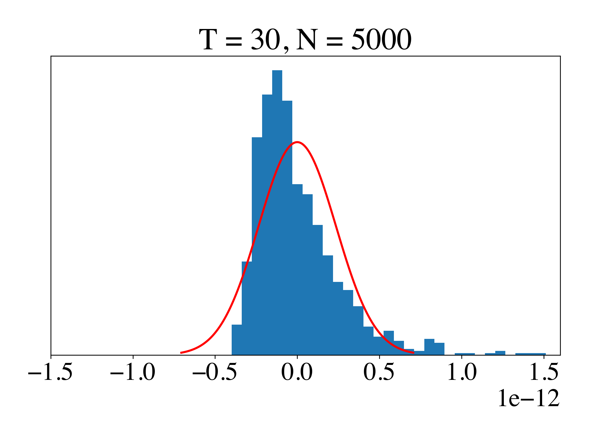
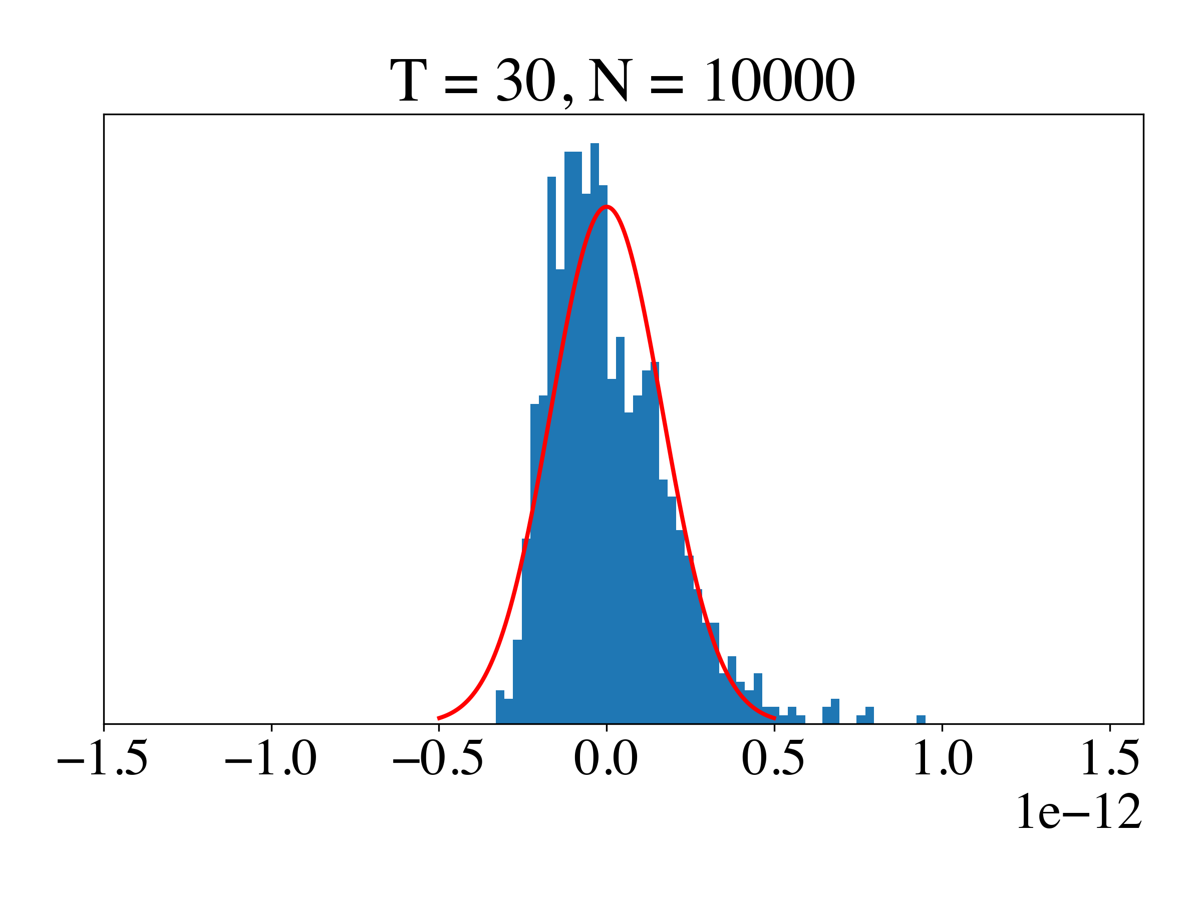
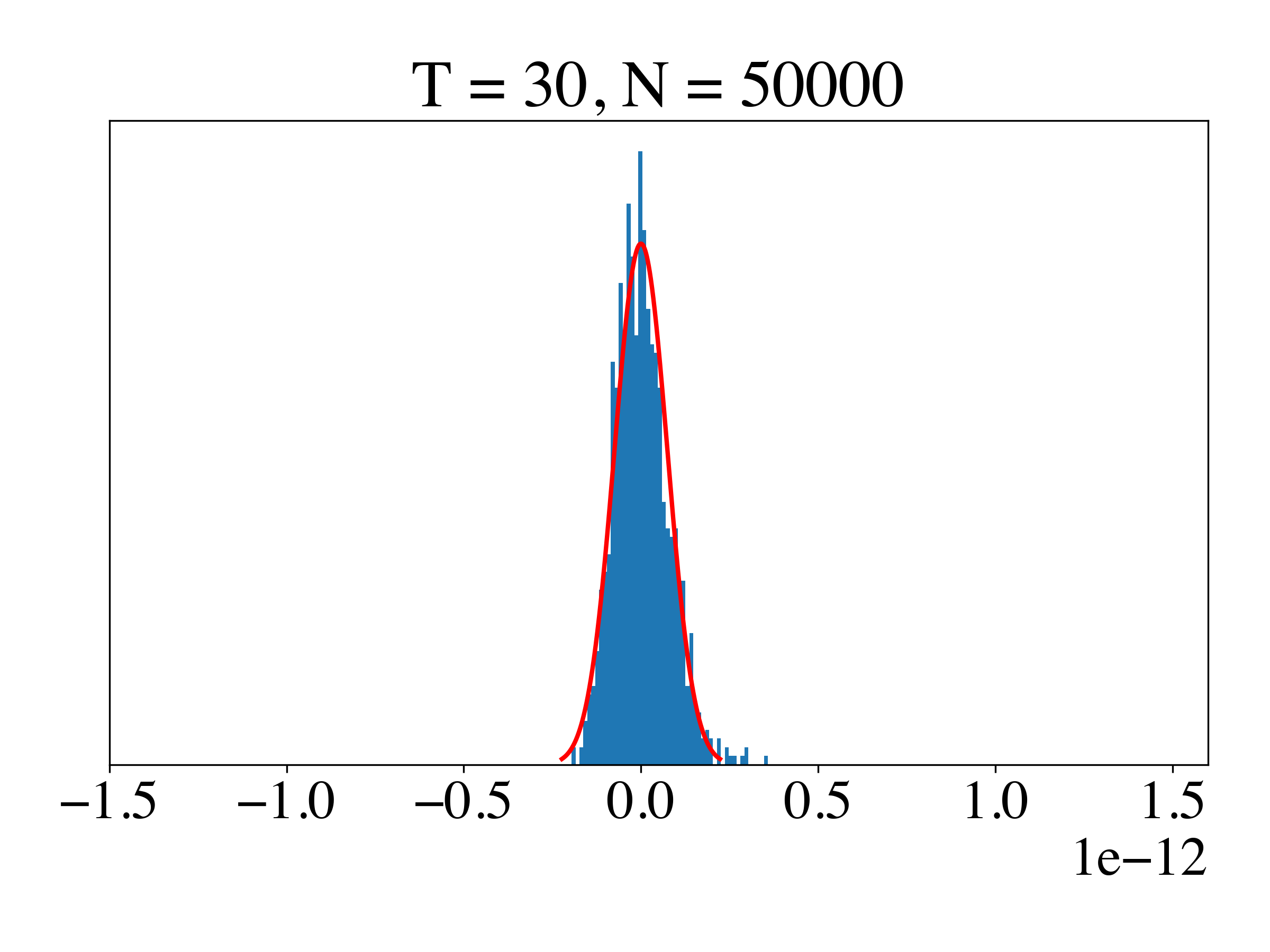
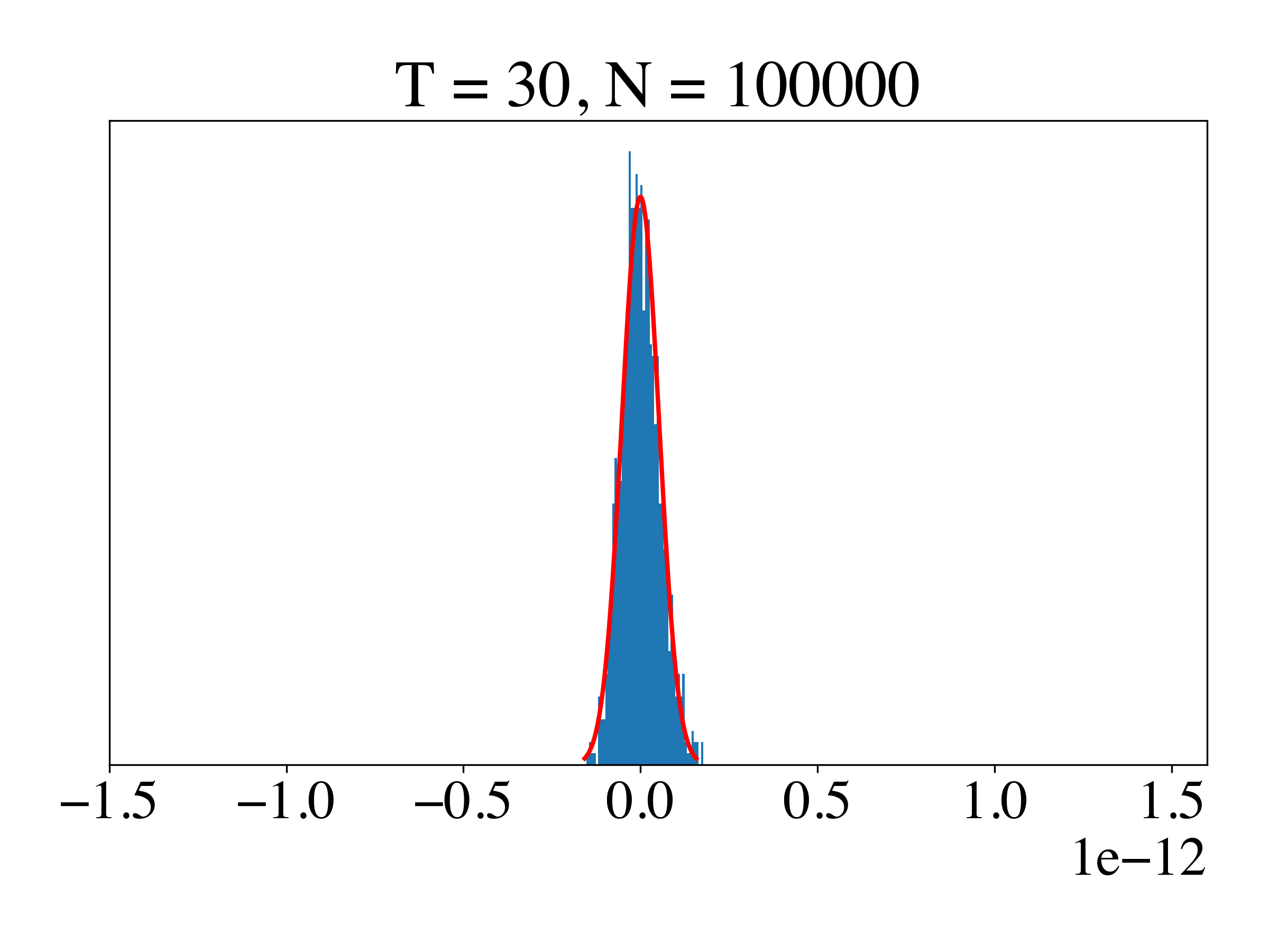
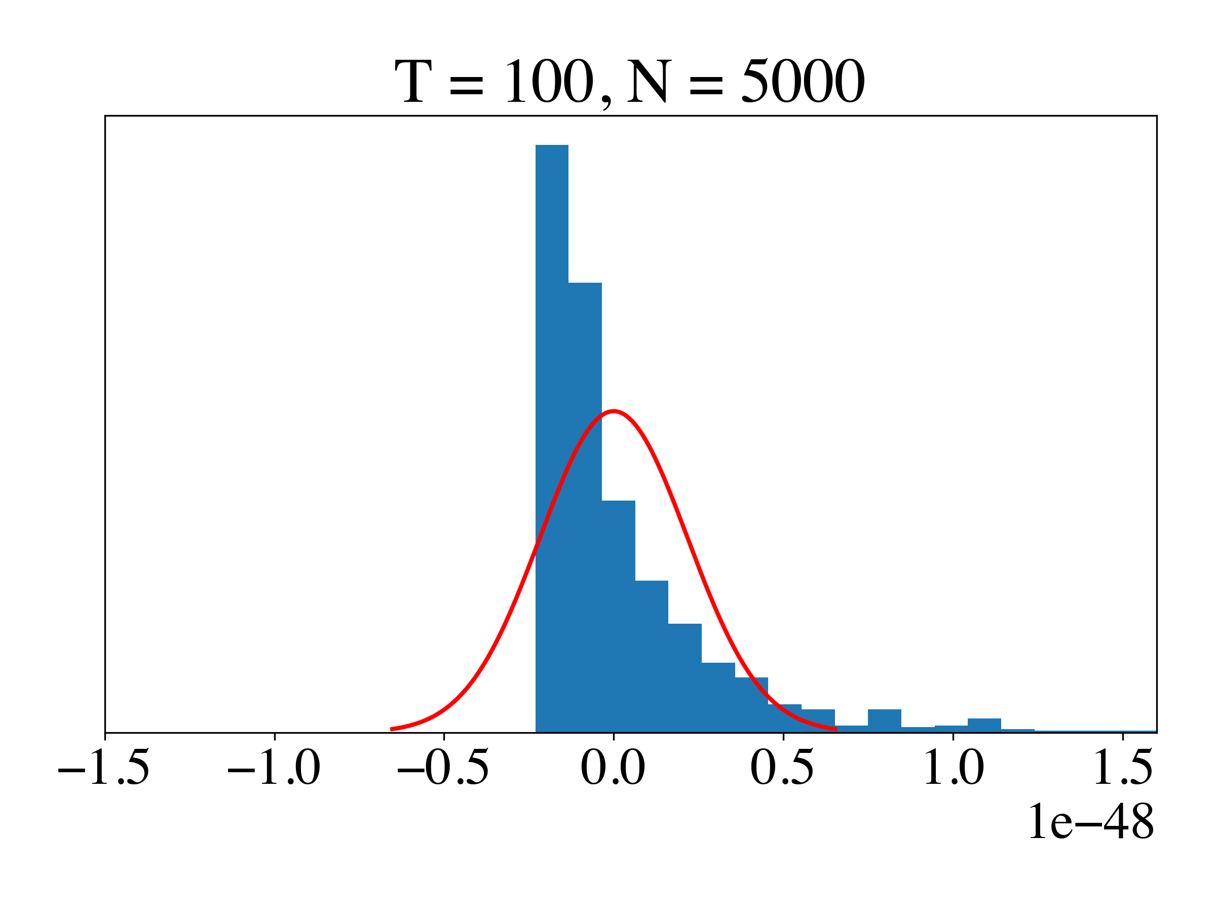
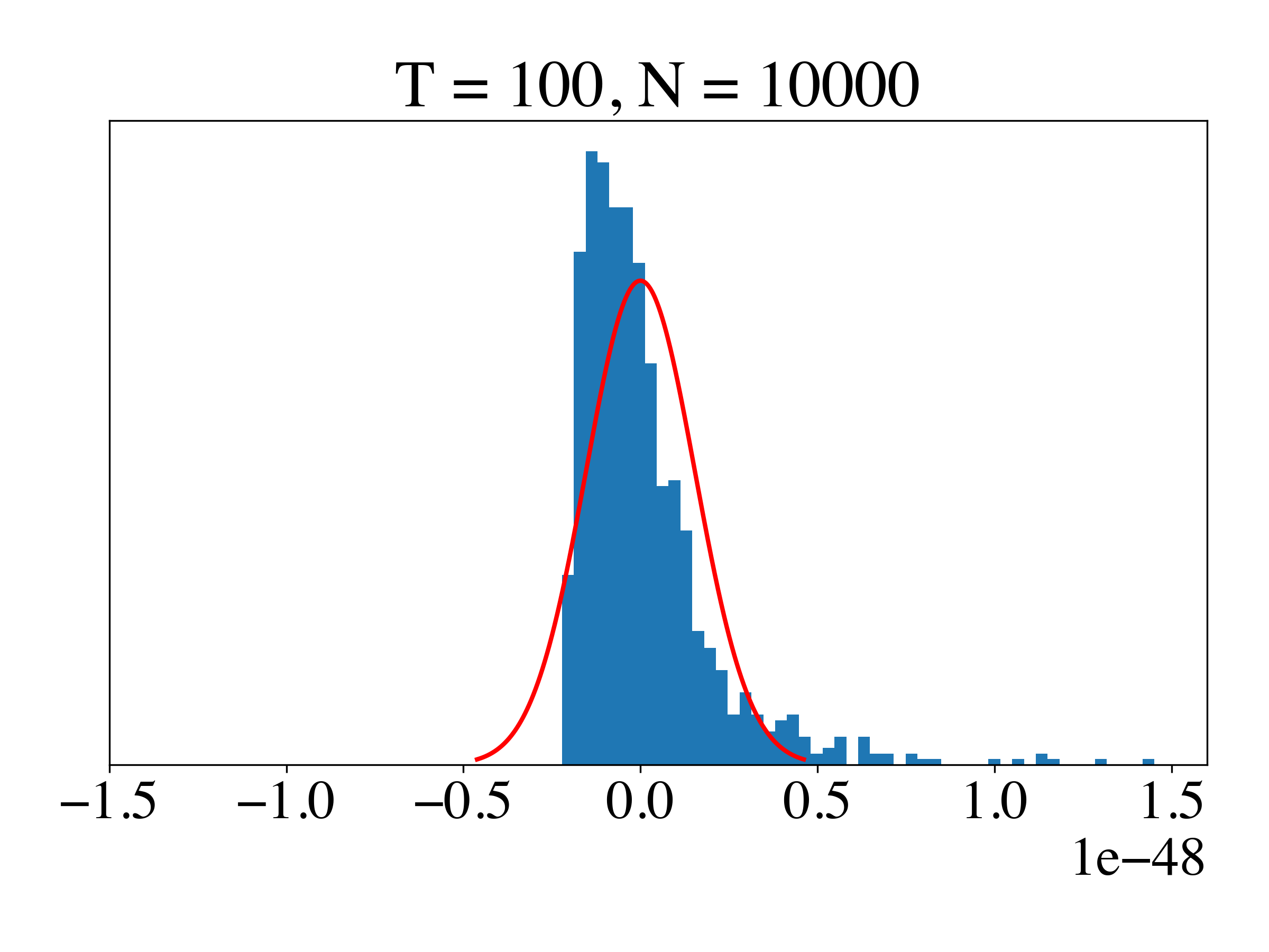
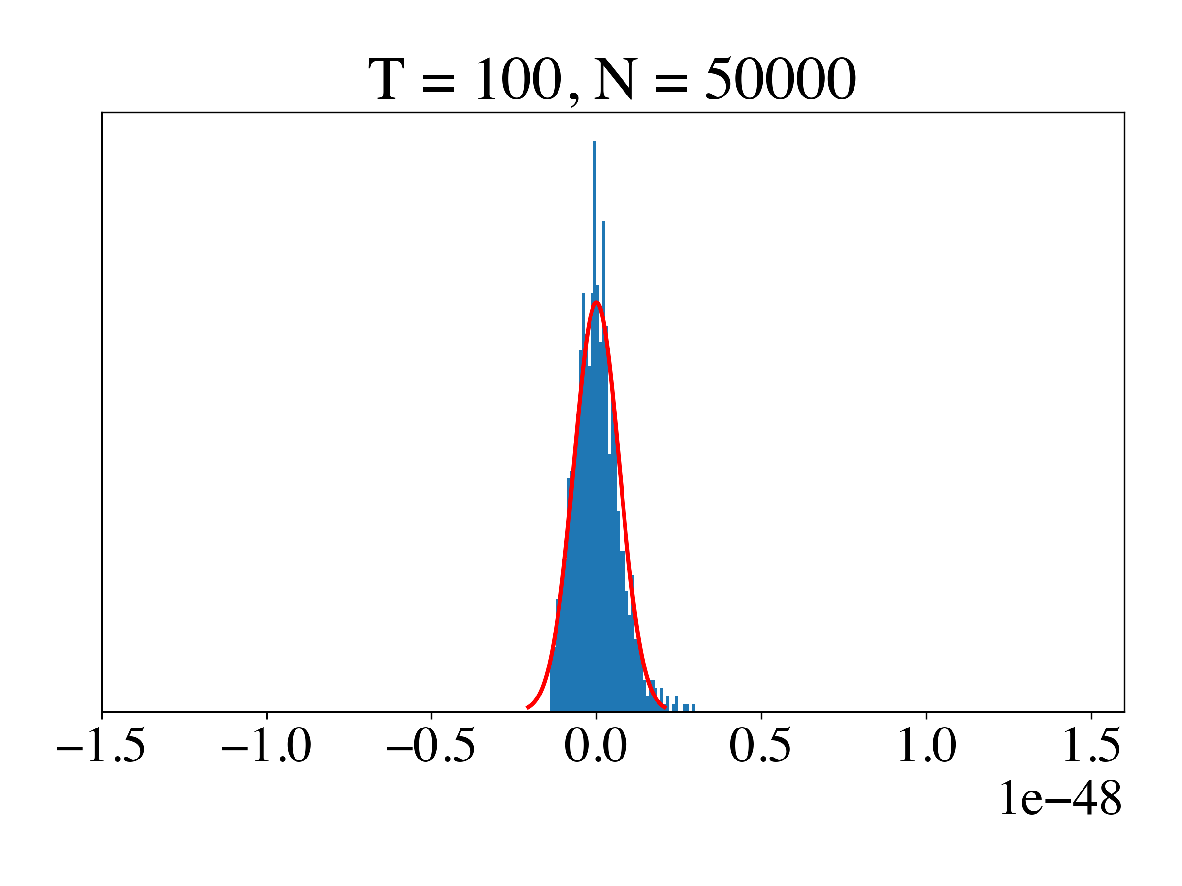
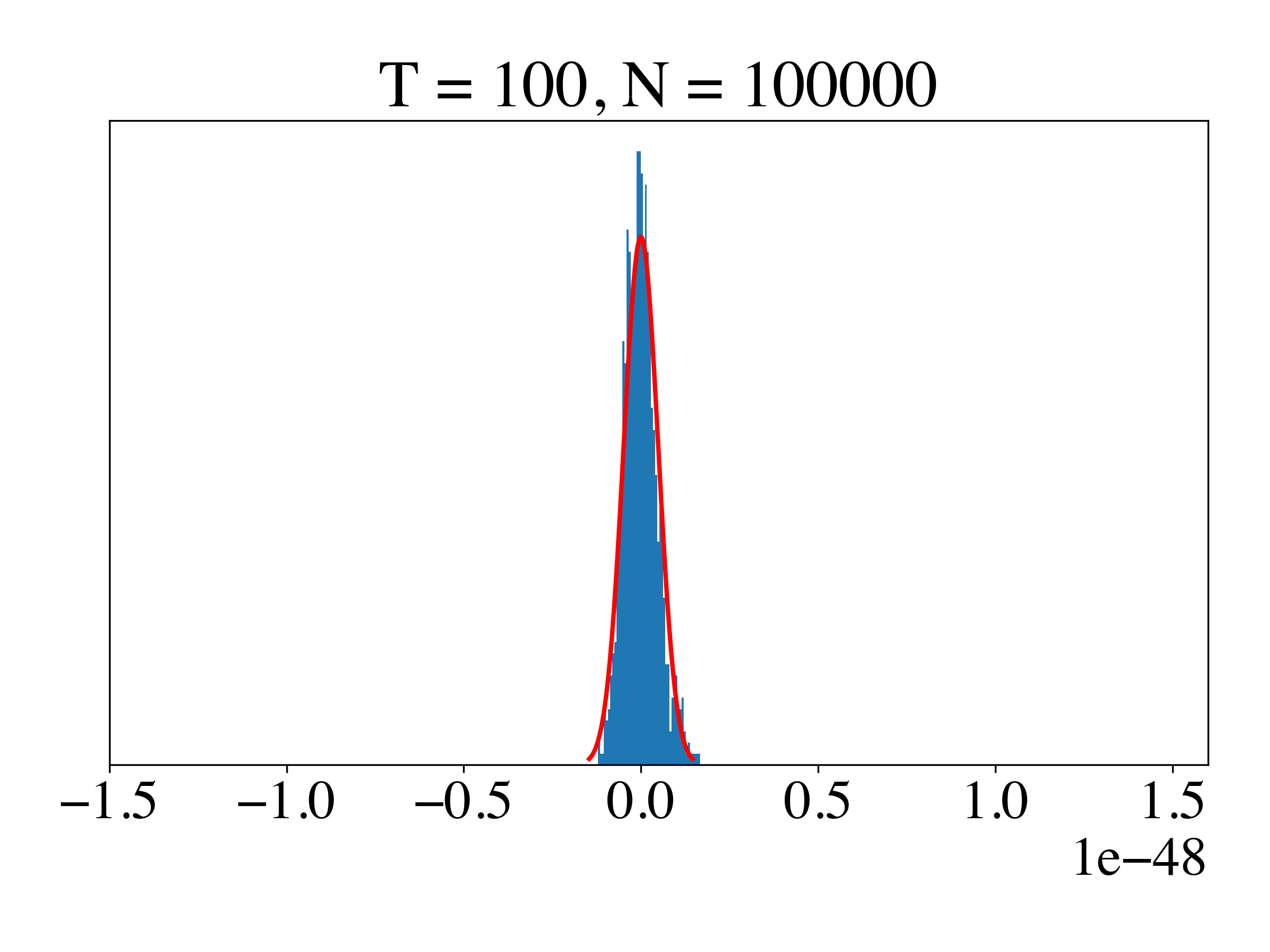
Figure 3: Empirical histograms of $\hat{P}r(x_{1:T})-Pr(x_{1:T})$ estimated under different training size $N$ and length $T$ and theoretical density calculated based on Theorem 1. Each subfigure is associated with a different $N$. As $N$ increases, the distribution converges to the theoretical normal distribution. Also, when $T$ is smaller, the estimation error converges more quickly to the asymptotic distribution.

(a) Likelihood estimation error from first-order first moment estimation.

(b) Likelihood estimation error from first-order second moment estimation.

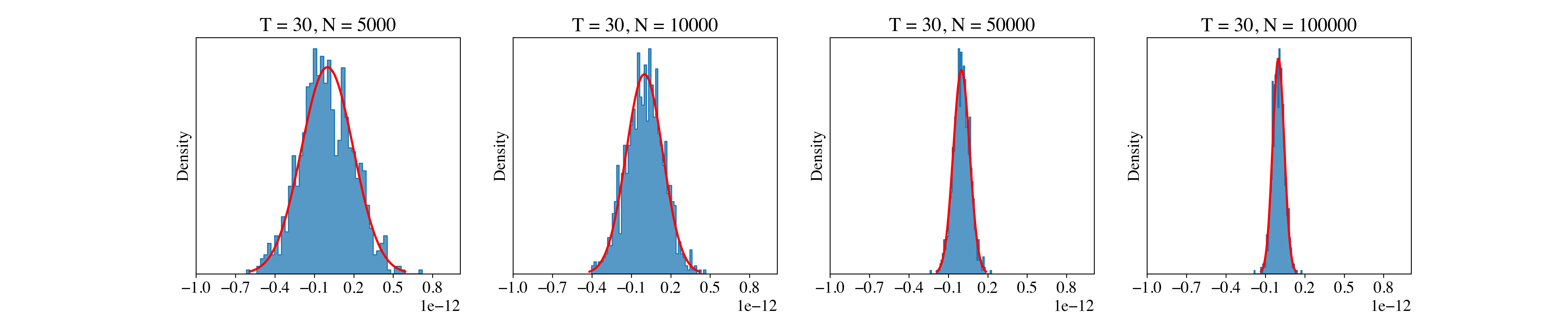
(c) Likelihood estimation error from first-order third moment estimation.

Figure 4: Histogram of the first-order error from the first, second and third moment estimation error (i.e. $(v+\tilde{v})^{\top}\widehat{\Delta\mu}$, $\sum_{t=0}^{T}b_{t}^{\top}\widehat{\Delta\Sigma}\tilde{b_{t}}$, and $\sum_{t=1}^{T}a_{t}^{\top}\widehat{\Delta K}(y_{t})\tilde{a_{t}}$) under different training sizes $N$ with fixed length $T=30$ vs. the theoretical pdf calculated based on Theorem 1 (red line). Each subfigure is associated with a different $N$. As $N$ increases, the distribution converges to the theoretical normal distribution.

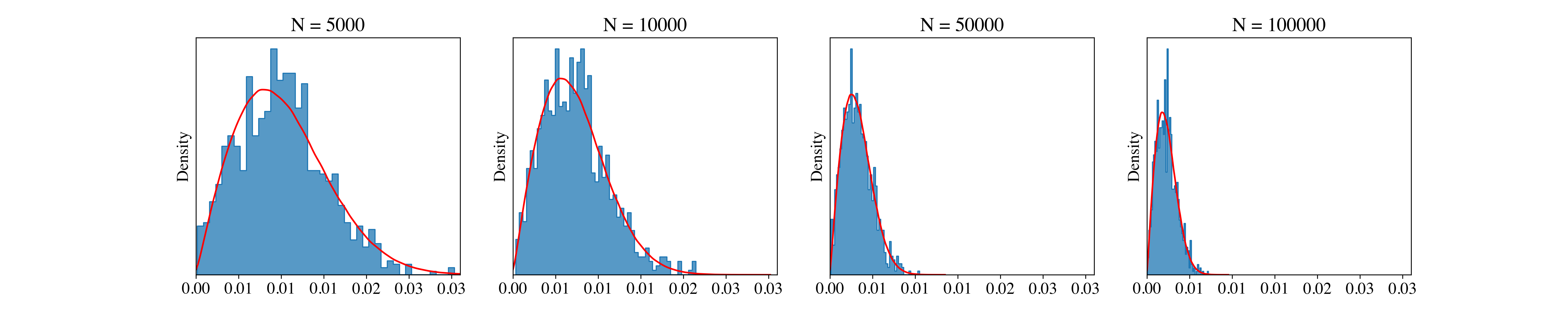
(a) Frobenius norm of first moment estimation.

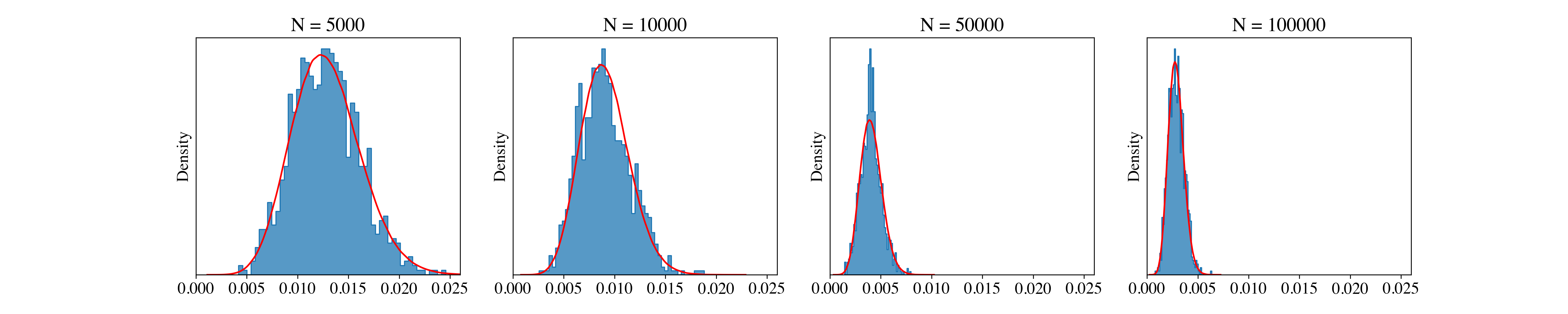
(b) Frobenius norm of second moment estimation.

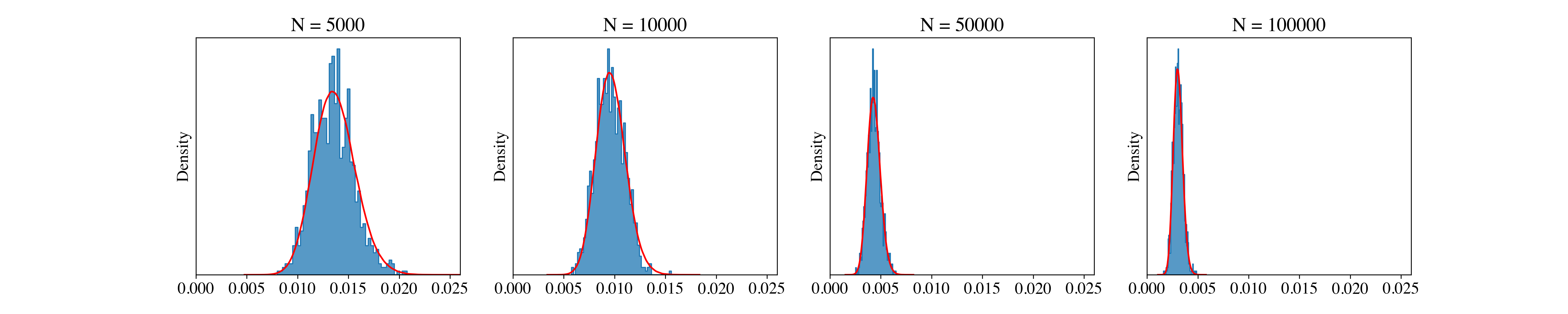
(c) Frobenius norm of third moment estimation error

Figure 5: Histogram of the Frobenius norm of the first, second and third moment estimation error (i.e. $\mu$, $\Sigma$ and $K$) under different training size $N$ vs. the theoretical pdf (red line). Here the red line is the theoretical Chi-squared distribution. Each subfigure is associated with a different $N$. As $N$ increases, the distribution converges to the theoretical distribution.

A brief aside: experimental validation of Theorem 1.

We performed a series of experiments to validate the conclusions of theorem 1. We generated a target series $x_{1:T}$ with $x_{i}\in\mathbb{R}^{3}$ and $T=30,100$ using a 3-state GHMM, where the initial probabilities and sticky transition probabilities are as described in Section 5.1.1, and with discrete emission probability matrix $[[0.8,0.1,0.1]^{\top},[0.1,0.8,0.1]^{\top},[0.1,0.1,0.8]^{\top}]^{\top}$. Parameters $\widehat{\mu},\widehat{\Sigma}$, and $\widehat{K}$ were estimated using training samples generated under the same model. Specifically, $N$ i.i.d. samples $Y_{1}^{(\mu)}$ were used to estimate $\widehat{\mu}$, $N$ i.i.d. samples of $(Y_{1}^{(\Sigma)},Y_{2}^{(\Sigma)})$ to estimate $\widehat{\Sigma}$, and $N$ i.i.d. samples of $(Y_{1}^{(K)},Y_{2}^{(K)},Y_{3}^{(K)})$ to estimate $\widehat{K}$. We chose training sets of size $N=5000,10000,50000,100000$ and for each $N$ we replicated the experiment 1000 times. For each replication, we estimated $\hat{P}r(x_{1:T})^{(N,r)}$ where $r$ indexes the replication. For each $N$, we construct the histogram v.s. theoretical probability density function (pdf) for the estimation error, i.e. $\{\hat{P}r(x_{1:T})^{(N,r)}\}_{r}$, which by Theorem 1 should converge to a normal distribution as $N$ grows larger. In Figure 3 we indeed see the desired effect. As $N$ grows larger we see that the distribution of the estimated likelihood converges to the normal distribution, and with a shorter length $T$, the error converges faster. We also separately analyzed the asymptotic behaviour of the first-order estimation error from first moment error, $(v+\tilde{v})^{\top}\widehat{\Delta\mu}$, second moment error, $\sum_{t=0}^{T}b_{t}^{\top}\widehat{\Delta\Sigma}\tilde{b_{t}}$, and third moment error, $\sum_{t=1}^{T}a_{t}^{\top}\widehat{\Delta K}(y_{t})\tilde{a_{t}}$ (as shown in Figure 4), and we found that the third moment estimation error dominates the error terms and has the largest contribution as shown in Table 1. We further analyzed the asymptotic distribution of the Frobenius norm of the first, second and third moment estimation error (i.e. $\mu$, $\Sigma$ and $K$). Figure 5 shows the empirical histogram and its corresponding theoretical pdf.

We note that there are two facets to the error when estimating the likelihood. The first stems from the typical CLT-type error in estimating the parameters of the model (i.e. for smaller $N$ the $\mathcal{O}_{p}(N^{-1})$ term is not small enough). The second is that any error introduced into the system from estimation error can propagate under forward recursion. To achieve a stable normal distribution given the second issue, $N$ must be much greater than $T$. In our simulation ($T=100$), at $N=10000$ we see reasonable evidence of asymptotic normality, while at $N=5000$ we do not. When $N=T$ or $N$ is only slightly larger than $T$, the distribution heavy-tailed. That is to say, there could be outliers. This also suggests us to add some kinds of regularization.

For simplicity of presentation, we derived Theorem 1 under the assumption that the output distribution is discrete. For continuous output, the CLT still holds with a proper kernel function $G(\cdot)$ as mentioned in section 1.2.

Error source	Mathematical expression	Theoretical std	Variance explained ratio
1st moment estimation	$(v+\tilde{v})^{\top}\widehat{\Delta\mu}$	$1.09\times 10^{-12}/\sqrt{N}$	$0.43\%$
2nd moment estimation	$\sum_{t=0}^{T}b_{t}^{\top}\widehat{\Delta\Sigma}\tilde{b_{t}}$	$8.98\times 10^{-12}/\sqrt{N}$	$29.21\%$
3rd moment estimation	$\sum_{t=1}^{T}a_{t}^{\top}\widehat{\Delta K}(y_{t})\tilde{a_{t}}$	$1.39\times 10^{-11}/\sqrt{N}$	$70.36\%$

(a) $T=30$.

Error source	Mathematical expression	Theoretical std	Variance explained ratio
1st moment estimation	$(v+\tilde{v})^{\top}\widehat{\Delta\mu}$	$2.66\times 10^{-49}/\sqrt{N}$	$0.30\%$
2nd moment estimation	$\sum_{t=0}^{T}b_{t}^{\top}\widehat{\Delta\Sigma}\tilde{b_{t}}$	$7.75\times 10^{-48}/\sqrt{N}$	$25.37\%$
3rd moment estimation	$\sum_{t=1}^{T}a_{t}^{\top}\widehat{\Delta K}(y_{t})\tilde{a_{t}}$	$1.33\times 10^{-47}/\sqrt{N}$	$74.59\%$

(b) $T=100$.

Table 1: Theoretical variance for first, second, third moment estimation errors based on simulated data with different $T$.

3 Projected SHMM

3.1 Motivation for Adding Projection

In the Baum-Welch algorithm (Baum et al.,, 1970), when we make a prediction, we are effectively predicting the belief probabilities, or weights, for each underlying hidden state. Denote the predicted weight vector at time $t$ as $\hat{w}_{t}$. Then the prediction can be expressed as a weighted combination of cluster means $\hat{y}_{t}=M\hat{w}_{t}$ where $||\hat{w}_{t}||_{1}=1$. The weights are explicitly guaranteed to be non-negative and sum to $1$ during forward propagation in the Baum-Welch algorithm, which is consistent with their physical meaning. However, these two constraints are not explicitly implemented in spectral estimation since SHMM doesn’t estimate the weights directly. Therefore, SHMM can sometimes give predictions which are far away from the polyhedron spanned by the cluster means. In order to solve this problem, we propose the projected SHMM, where projection serves to regularize the predictions to be within a reasonable range.

This is particularly important when $N$ is not sufficiently large, and extreme deviations of the estimated likelihood from the true likelihood can occur when error is propagated over time. Regularization can help stabilize the performance of estimation of the likelihood by limiting this propagation of error.

3.2 Projection-onto-polyhedron and Projection-onto-Simplex SHMM

There are two ways to achieve projection for our problem: projection-onto-polyhedron and projection-onto-simplex. Projection-onto-polyhedron is derived directly from the motivation for using projections in SHMM, but suffers from high computational cost. To obtain a better computational performance, we propose projection-onto-simplex as an alternative.

3.2.1 Projection-onto-Polyhedron

Projection-onto-polyhedron SHMM first generates prediction $\hat{y}_{t}^{(SHMM)}$ through the standard SHMM and then projects it onto the polyhedron with vertices $\widehat{M}$. In other words, we find the point on the polyhedron spanned by $\widehat{M}$ that is nearest to the predicted $\hat{y}_{t}^{(SHMM)}$. We can use any distance to define “nearest point” but in our exposition we use Euclidean distance. Mathematically, we substitute the recursive forecasting in Eq 3 with

$$\hat{y}_{t}^{(SHMM)} = \frac{C(y_{t-1})\hat{y}_{t-1}}{c^{\top}_{\infty}C(y_{t-1})\hat{y}_{t-1}};$$

$$\hat{y}_{t} = \operatorname*{\arg\min}_{y\in Poly(\widehat{M})}d(y,\hat{y}_{t}^{(SHMM)}),$$ (6)

where $d(\cdot,\cdot)$ is the distance function (such as Euclidean distance), and

$$Poly(\widehat{M})=\{y=\widehat{M}w|w\ is\ on\ the\ simplex\}$$

is the polyhedron with vertices $\widehat{M}$. This results in a convex optimization problem if the distance is convex, which is true for general distance functions such as Euclidean distance. We can solve this using standard convex optimization methods such as the Newton-Raphson algorithm (Boyd et al.,, 2004), with variants allowing linear constraints such as the log-barrier methods (Frisch,, 1955). To the best of our knowledge, there is no dedicated algorithm for solving projection-onto-polyhedron, and unfortunately finding a fast solution seems to be challenging. The approach we take is to write the loss function of the constrained problem as the loss function with an indicator function, and use the log-barrier method to approximate the linear constraints through log-barrier functions. We then use the Newton-Raphson algorithm to optimize this approximated loss function, iteratively relaxing the approximation and solving it until convergence. Note that this optimization must be done at every time step. This implies a trade-off between the accuracy of the approximation and optimization. Recall that we turn to SHMM because it is faster than the Baum-Welch algorithm, so any modification should not slow down the computation too much, otherwise this mitigates one of its strong advantages.

3.2.2 Projection-onto-Simplex

To obtain higher efficiency in computation, we propose a second projection regularization method: projection-onto-simplex. It leverages an algorithm that allows us to calculate the projection with time complexity $\mathcal{O}(d\log(d))$ (Wang and Carreira-Perpinán,, 2013). To avoid projection onto a polyhedron, we leverage the fact that $\hat{y}_{t}=\widehat{M}\hat{w}_{t}$ and optimize over $\hat{w}_{t}$ which lies on the simplex. Mathematically, the optimization problem becomes

$$\hat{w}_{t} = \operatorname*{\arg\min}_{w\in Simplex}||w-\widehat{M}^{-1}\hat{y}_{t}^{(SHMM)}||_{2}^{2}.$$ (7)

This solution is not equivalent to solution from the projection-onto-polyhedron, because $d(a,b)\neq d(Aa,Ab)$ in general. However, the solution set is the same, i.e. the predictions are both guaranteed to be constrained to the polyhedron. The solution of Eq 7 can be obtained through a closed-form solution provided in Algorithm 1, which avoids iterations during convex optimization, yielding fast estimation. Figure 6 gives a graphical demonstration for the projection-onto-polyhedron and projection-onto-simplex methods.

Input : $u=[u_{1},u_{2},\cdots,u_{d}]^{\top}$

Sort $u$ into $z$: $z_{1}\geq z_{2}\cdots\geq z_{d}$;

Find $\rho=max\{1\leq i\leq d:z_{i}+\frac{1}{i}(1-\sum_{j=1}^{i}z_{j})>0\}$;

Define $\lambda=\frac{1}{\rho}(1-\sum_{j=1}^{\rho}z_{j})$;

Solve $u^{(proj)}$, s.t. $u_{i}^{(proj)}=max(u_{i}+\lambda,0)$, $i=1,\cdots,d$;

Output : $u^{(proj)}$

Algorithm 1 Projection-onto-simplex (Wang and Carreira-Perpinán,, 2013).

The full projected SHMM algorithm is shown in Algorithm 2. In Algorithm 2, Steps 1-3 are identical to the standard SHMM. Steps 4-5 estimate $\hat{M}$ by Gaussian Mixture Models (GMM) (McLachlan and Basford,, 1988), calculate the weight processes $\{w_{t}\}$, and apply SHMM on the weight process. Step 6 applies projection-onto-simplex on the recursive forecasting. Step 7 projects the data back into the original space.

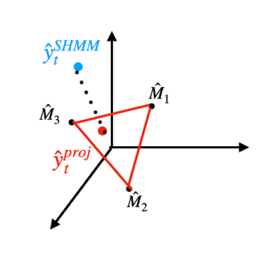
(a) Projection-onto-polyhedron.

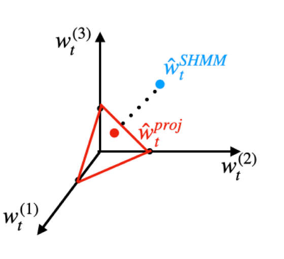
(b) Projection-onto-simplex.

Figure 6: The left figure shows the projection-onto-polyhedron step, and the right shows projection-onto-simplex. In both methods, we project the predicted values (blue points) into the constrained regions (defined with a red boundary), a polyhedron (left) or simplex (right).

Input : $\{x_{t}\}$, where $t=1,\cdots,T$

Output : $\hat{x}_{T+1}$

Step 1: Compute $\hat{E}[x_{t+1}\otimes x_{t}]=\frac{1}{T-2}\sum_{i=1}^{T-2}x_{t+1}x_{t}^{\top}$;

Step 2: Obtain $\hat{U}$ by extracting the first $k$ left eigenvectors of $\hat{E}[x_{t+1}\otimes x_{t}]$;

Step 3: Reduce dimensionality $y_{t}=\hat{U}^{\top}x_{t}$;

Step 4: Estimate cluster mean by GMM, and obtain $\hat{M}$, where each column is the mean vector of each cluster. Then the weight vector is $w_{t}=\hat{M}^{-1}y_{t}$ for $t=1,\cdots,T$;

Step 5: Calculate $\hat{\mu}=\frac{1}{T}\sum_{t=1}^{\top}w_{t}$, $\hat{\Sigma}=\frac{1}{T-1}\sum_{t=1}^{T-1}w_{t+1}w_{t}^{\top}$, and $\hat{K}=\frac{1}{T-2}\sum_{t=1}^{T-2}w_{t+2}\otimes w_{t}\otimes w_{t+1}$. Set $\hat{c}_{1}=\hat{\mu}$, $\hat{c}_{\infty}^{\top}=c_{1}^{\top}\hat{\Sigma}^{-1}$, and $\hat{C}(w_{t})=\hat{K}(w_{t})\hat{\Sigma}^{-1}$;

Step 6: Recursive prediction with projection-onto-simplex $\hat{w}_{t}=Proj\left(\frac{\hat{C}(w_{t-1})\hat{w}_{t-1}}{\hat{c}^{\top}_{\infty}\hat{C}(w_{t-1})\hat{w}_{t-1}}\right)$ for $t=2,\cdots,T+1$ where $Proj(a)=\operatorname*{\arg\min}_{w\in Simplex}||w-a||_{2}^{2}$ can be solved by Algorithm 1, and set $\hat{y}_{1}=\hat{c}_{1}$;

Step 7: $\hat{x}_{T+1}=\hat{U}\hat{y}_{T+1}=\hat{U}\hat{M}\hat{w}_{T+1}$;

Algorithm 2 Projection-onto-simplex SHMM.

3.2.3 Bias-variance tradeoff

In PSHMM, we leverage GMM to provide projection boundaries, which would introduce bias, since the hidden state means estimated by GMM are biased where we ignore time dependency information. In addition, either projection method– ’projection-onto-polyhedron’ or ’projection-onto-simplex’– can introduce bias since they are not necessarily an orthogonal projection due to optimization constraints. However, adding such a projection will largely reduce the variance. That is, there is a bias-variance tradeoff.

3.3 Discussion of the proposed methodology

In this section, we discuss considerations for the proposed methodology. In addition to the choice of dimensionality of the projection space, we discuss computation of the projection matrix $U$. Finally, we show how to adapt the method when the dimensionality of the projection space $d$ is believe to be higher than the observation space. In this case, we provide a mechanism based on initially estimating a GMM on the observations directly to obtain a suitable mapping from the observation space to the projection space.

3.3.1 The choice of hyperparameter $d$

$d$ is the dimensionality of the projection space. In theory, $d$ should equal the number of states in the HMM. Our simulations show that when $d$ is chosen to be equal to the underlying true number of states, the estimation and prediction will perform better than at other values of $d$. However, the number of hidden states is usually unknown. In practice, we can either choose $d$ using prior knowledge or tune it if we do not have a strong prior belief.

3.3.2 Calculation of $U$ matrix under extremely high-dimensional data: unigram or bigram randomized SVD

The projection matrix $U$ is constructed by the first $d$ left singular vectors from the singular value decomposition (SVD) (Eckart and Young,, 1936) of the bigram covariance matrix $\widehat{\Sigma}=\widehat{\mathrm{E}}[X_{2}\otimes X_{1}]$. This encodes the transition information and will eliminate the in-cluster covariance structure. However, this is not the only acceptable projection. For instance, we could also estimate $U$ through an SVD of $\widehat{\mathrm{E}}[X_{1}\otimes X_{1}]$. This will encode covariance structure along with information about the cluster means. In most cases we suggest using the bigram matrix.

A point worth mentioning is that for extremely high-dimensional cases, we can leverage a fast approximation algorithm for computing $\hat{U}$. The algorithm is based on the randomized SVD (Halko et al.,, 2011). When computing the SVD of the bigram matrix, we need to avoid computing the covariance matrix $\hat{E}[x_{t+1}\otimes x_{t}]$. The standard algorithm for the SVD requires time complexity $\mathcal{O}(Tp^{2}+p^{3})$, where $T$ and $p$ are the sample size and dimensionality of the dataset. For the high-dimensional cases where $p\gg d$, the randomized SVD has time complexity $\mathcal{O}(pT\log(d)+(p+T)d^{2})$. In this case, the bottleneck is the computation of $\hat{E}[x_{t+1}\otimes x_{t}]$, whose time complexity is $\mathcal{O}(Tp^{2})$.

Note that $\hat{E}[x_{t+1}\otimes x_{t}]=\frac{1}{T-2}\sum_{i=1}^{T-2}x_{t+1}x_{t}^{\top}=\frac{1}{T-2}X_{2}^{\top}X_{1}$, where $X_{2}=[x_{2},\cdots,x_{T}]^{\top}$ and $X_{1}=[x_{1},\cdots,x_{T-1}]^{\top}$. We can take the randomized SVD of $X_{1}$ and $X_{2}$ separately to obtain two rank-$\tilde{d}$ decompositions with $d\leq\tilde{d}\ll p$: $X_{1}\approx U_{1}\Sigma_{1}V_{1}^{\top}$, $X_{2}\approx U_{2}\Sigma_{2}V_{2}^{\top}$. Then $X_{2}^{\top}X_{1}=V_{2}(\Sigma_{2}U_{2}^{\top}U_{1}\Sigma_{1})V_{1}^{\top}$. The matrix $(\Sigma_{2}U_{2}^{\top}U_{1}\Sigma_{1})$ is of dimension $\tilde{d}\times\tilde{d}$, and computing it is much faster than computing $\hat{E}[x_{t+1}\otimes x_{t}]$. We then perform an SVD on this matrix to get $\Sigma_{2}U_{2}^{\top}U_{1}\Sigma_{1}=\tilde{U}\tilde{\Sigma}\tilde{V}^{\top}$. Then $\hat{E}[x_{t+1}\otimes x_{t}]\approx(V_{2}\tilde{U})(\frac{1}{T-2}\tilde{\Sigma})(V_{1}\tilde{V})^{\top}$. Note that $V_{2}\tilde{U}$ and $V_{1}\tilde{V}$ are orthonormal matrices and $\frac{1}{T-2}\tilde{\Sigma}$ is a diagonal matrix, so this is the rank-$\tilde{d}$ SVD of $\hat{E}[x_{t+1}\otimes x_{t}]$. The first $d$ vectors of $V_{2}\tilde{U}$ are an estimate of the $\hat{U}$ matrix we are to compute in Step 1 and 2 in Algorithm 2.

3.3.3 Projecting $\{w_{t}\}$ onto the probability space

The standard SHMM and the proposed PSHMM perform well under the high-dimensional observations. They will fail when the dimensionality of the projection space $d$ is believe to be higher than the observation space. In this setting, we must increase the dimensionality of the observations in order to avoid low-rank issues for moment estimation of $\Sigma$ which needs to be inverted. One way to increase the dimensionality is to project observations onto a Hilbert space using kernel methods (Song et al.,, 2010). However, this method suffers from lack of interpretability.

We propose to project the observations directly onto the assumed probability space to increase the dimensionality. Taking cues from the advantages of PSHMM, we fit a GMM on our observations $x_{t}$ to obtain observation representations $w^{(i)}_{t}=\mathrm{P}(h_{t}=i|x_{t})$. This probability vector has similar interpretation to the emission probability in the Gaussian HMM but is computed by GMM. Specifically, we modify steps 2 and 4 in Algorithm 2 as follows:

• Step 2: Set $\hat{U}$ to be the identity matrix so that $y_{t}=x_{t}$ for all $t$;

• Step 4: Estimate GMM to obtain $\hat{M}$ and $w_{t}=[w_{t}^{(1)},w_{t}^{(2)},\cdots,w_{t}^{(d)}]^{\top}$ for each $t$, where each $w_{t}^{(i)}=\mathrm{P}(h_{t}=i|y_{t})$ is from GMM.

The above modifications are equivalent to directly computing probabilities from the GMM in $x$-space, skipping steps 1 to 4 altogether. However, in order to draw a direct comparison to our proposed method in the high-dimensional setting, we chose to modify particular steps of algorithm 2 to achieve our goal.

Compared to Song et al., (2010), the advantage of this method lies in its interpretation. In this model, $w_{t}$ has a straightforward probabilistic meaning, i.e. the weight on different components for a given observation. The SHMM directly predicts $w_{t}$, or the weight process. Because we still leverage GMM and project predictions onto the probability space, the bias-variance tradeoff (see Section 3.2.3) still exists.

4 Online Learning

Because computational speed is an important consideration when leveraging SHMMs, it is natural to consider online learning for SHMMs to further accelerate the computational speed in some settings. Traditionally SHMMs will be estimated using batch or offline learning. Batch learning is applicable under the following assumptions: (1) the entire training data set is available in the training phase (2) we can endure a relative long computational time and (3) the underlying data generation mechanism is consistent in both the training and forecasting phases (Fontenla-Romero et al.,, 2013). However, there are many application scenarios that do not meet those assumptions. For example, in quantitative trading, markets often exhibit a regime-switching phenomenon. Thus it is likely that the observed returns for some financial products are not stationary. In high frequency trading, especially in second-level or minute-level trading, the delay from frequent offline re-training of the statistical model could impact the strategy and trading speed (Lahmiri and Bekiros,, 2021).

4.1 Online Learning of SHMM and PSHMM

SHMM and PSHMM can be useful in online settings, and the ability to adapt the parameters is essential. Let $\hat{\mu},\hat{\Sigma}$, and $\hat{K}$, be the estimated moments based on $T$ data points.

When we obtain new data $Y_{T+1}$, we update our moments recursively as follows:

$$\hat{\mu} \xleftarrow{} \frac{T\cdot\hat{\mu}+Y_{T+1}}{T+1};$$

$$\hat{\Sigma} \xleftarrow{} \frac{(T-1)\cdot\hat{\Sigma}+Y_{T+1}\otimes Y_{T}}{T};$$

$$\hat{K} \xleftarrow{} \frac{(T-2)\cdot\hat{K}+Y_{T+1}\otimes Y_{T-1}\otimes Y_{T}}{T-1};$$

$$T \xleftarrow{} T+1.$$ (8)

The above works for both SHMM and PSHMM. The pseudo code for the online learning of PSHMM is shown in Algorithm 3.

Input : $\{x_{t}\}_{t=1,\cdots,T}$, the warm-up length $T_{warmup}$

Output : $\{\hat{x}_{t}\}_{t=T_{warmup}+1}^{T+1}$ yielded sequentially.

Step 1: Compute $\hat{E}[x_{t+1}\otimes x_{t}]^{(warmup)}=\frac{1}{T_{warmup}-2}\sum_{i=1}^{T_{warmup}-2}x_{t+1}x_{t}^{\top}$;

Step 2: Obtain $\hat{U}$ by extracting the first $k$ left eigenvectors of $\hat{E}[x_{t+1}\otimes x_{t}]^{(warmup)}$;

Step 3: Reduce dimensionality $y_{t}=\hat{U}^{\top}x_{t}$ for $t=1,\cdots,T_{warmup}$;

Step 4: Estimate cluster mean by GMM by data $\{\hat{y}_{t}\}_{t=1}^{T_{warmup}}$, and obtain $\hat{M}$, where each column is the mean vector of each cluster. Then the weight vector is $w_{t}=\hat{M}^{-1}y_{t}$ for $t=1,\cdots,T_{warmup}$;

Step 5: Calculate $\hat{\mu}$, $\hat{\Sigma}$, $\hat{K}$, $\hat{c}_{1}$, $\hat{c}_{\infty}^{\top}$ and $\hat{C}(\cdot)$ as described in Step 5 of Algorithm 2;

Step 6: Recursive prediction with projection-onto-simplex $\hat{w}_{t}$ for $t=1,\cdots,T_{warmup}+1$ as described in Step 6 of Algorithm 2. Yield $\hat{x}_{T_{warmup}+1}=\hat{U}\hat{M}\hat{w}_{T_{warmup}+1}$;

Step 7 (online learning and prediction):

for $t\leftarrow T_{warmup}+1$ to $T$ do

      

      $w_{t}=\hat{M}^{-1}\hat{U}^{\top}x_{t}$;

      

      Update $\hat{\mu}$, $\hat{\Sigma}$ and $\hat{K}$ according to Eq 8;

      

      Predict $\hat{w}_{t+1}$ by $\hat{w}_{t+1}=Proj\left(\frac{\hat{C}(w_{t})\hat{w}_{t}}{\hat{c}^{\top}_{\infty}\hat{C}(w_{t})\hat{w}_{t}}\right)$, where $\hat{C}(\cdot)$ and $\hat{c}^{\top}_{\infty}$ are based on updated $\hat{\mu}$, $\hat{\Sigma}$ and $\hat{K}$, and $Proj(\cdot)$ is solved by Algorithm 1;

      

      Yield $\hat{x}_{t+1}=\hat{U}\hat{M}\hat{w}_{t+1}$;

      

end for

Algorithm 3 Online learning projection-onto-simplex SHMM.

Updating the GMM used in PSHMM

To update the first, second and third order moments of $w_{t}$, we replace $Y$ with $w$ in the above formulas. At question is if we also update the parameters of the GMM. There are several ways to do this. If desired, we recommend updating the GMM without changing cluster membership. For example, we can simply classify a new input into a particular cluster and update the cluster’s mean and covariance. In particular, we don’t suggest re-estimating the GMM to allow for adding or removing clusters. In theory, the number of clusters should be pre-specified to equal to the number of states in the HMM, which in turn specifies the dimensionality of space for $y$. The addition or deletion of a cluster in GMM fundamentally changes the relationship between the dimensionality of $y$ and the number of hidden states. In practice however, we find that PSHMM works well without any updates to the GMM.

4.2 Online Learning of SHMM Class with Forgetfulness

When dealing with nonstationary data, adding a forgetting mechanism on parameter estimation can be beneficial. We must specify a decay factor $\gamma$ that specifies the rate, $1-\gamma$, at which information is forgotten. The the updating rule is, then,

$$\hat{\mu} \xleftarrow{} \frac{(1-\gamma)\tilde{T}\hat{\mu}+Y_{T+1}}{(1-\gamma)\tilde{T}+1};$$

$$\hat{\Sigma} \xleftarrow{} \frac{(1-\gamma)\tilde{T}\hat{\Sigma}+Y_{T+1}\otimes Y_{T}}{(1-\gamma)\tilde{T}+1};$$

$$\hat{K} \xleftarrow{} \frac{(1-\gamma)\tilde{T}\hat{K}+Y_{T+1}\otimes Y_{T-1}\otimes Y_{T}}{(1-\gamma)\tilde{T}+1};$$

$$\tilde{T} \xleftarrow{} \tilde{T}\cdot(1-\gamma)+1.$$ (9)

Here $\tilde{T}=\sum_{i=1}^{T}(1-\gamma)^{i-1}$ serves as an effective sample size. This strategy is equivalent to calculating the exponentially weighted moving average for each parameter:

$$\hat{\mu}=\frac{\sum_{t=1}^{T}(1-\gamma)^{T-t}Y_{t}}{\sum_{t=1}^{T}(1-\gamma)^{T-t}};\hat{\Sigma}=\frac{\sum_{t=2}^{T}(1-\gamma)^{T-t}Y_{t}\otimes Y_{t-1}}{\sum_{t=2}^{T}(1-\gamma)^{T-t}};\hat{K}=\frac{\sum_{t=3}^{T}(1-\gamma)^{T-t}Y_{t}\otimes Y_{t-2}\otimes Y_{t-1}}{\sum_{t=3}^{T}(1-\gamma)^{T-t}}.$$ (10)

5 Simulations

5.1 Test Robustness under Different Signal-Noise Ratio, Mis-specified Models and Heavy-Tailed Data

5.1.1 Experiment setting

We generated $100$-dimensional data with length $10000$ for training data and $100$ for testing data under different settings, and used SHMM and PSHMM with recursive prediction for time series forecasting. We repeated each simulation setup $100$ times, calculated $R^{2}$ for each repeat, and computed an average $R^{2}$ over all repeats. The results below show this averaged $R^{2}$. We tested 3 variants of the PSHMM: projection onto polyhedron, projection onto simplex, and projection onto simplex with online learning. The online learning variant of PSHMM used $1000$ training samples for the initial estimate (warm-up), and incorporated the remaining $9000$ training samples using online updates. In our simulations, online training for PSHMM differs from offline training for two reasons. First, the estimation of $\hat{U}$ and $\hat{M}$ are based only on the warm-up set for online learning (as is the case for the online version of SHMM), and the entire training set for offline learning. Second, during the training period, for PSHMM, the updated moments are based on the recursive predictions of $\hat{w}_{t}$, which are themselves based on the weights $\{w_{s}\}_{s=1}^{t-1}$. For offline learning of PSHMM in contrast, the weights used to calculate the moments are based on the GMM estimates from the entire training dataset. For each state, we assumed the emission distribution has a one-hot mean vector and diagonal covariance matrix, that the mean vector of the $i$-th state is $[\mathrm{1}\{i=j\}]_{j=1}^{p}$ where $\mathrm{1}\{\cdot\}$ is the indicator function. We tested those methods and the E-M algorithm under two types of transition matrix, three different signal-noise ratios and different emission distributions as below:

• Transition matrix:

  • Sticky transition matrix: diagonal elements are $0.6$, off-diagonal elements are $\frac{0.4}{S-1}$, where $S$ is the hypyerparameter that tell how many clusters that generated the data;

  • Non-sticky transition matrix: diagonal elements are $0.4$, off-diagonal elements are $\frac{0.6}{S-1}$.

• Signal-noise ratio: The covariance matrix of each cluster is: $\sigma^{2}I_{p}$, where $p$ is the dimension of the space, $\sigma=0.01,0.05,0.1,0.5,1.0$.

• Data generated from:

  • Gaussian distribution: generate according to mean vector and covariance matrix;

  • $t$ distribution: generate standard a random vector of $i.i.d.$ $t_{5}$, $t_{10}$, $t_{15}$ and $t_{20}$ distribution first, and then multiply by covariance matrix and shifted by mean vector.

For each setting, we also showed the oracle $R^{2}$. To calculate the oracle, we assume we know all parameters for the HMM but do not know the specific hidden state at each time point.

5.1.2 Simulation Results

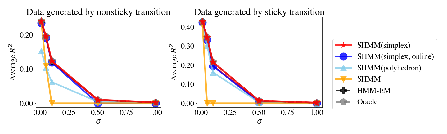
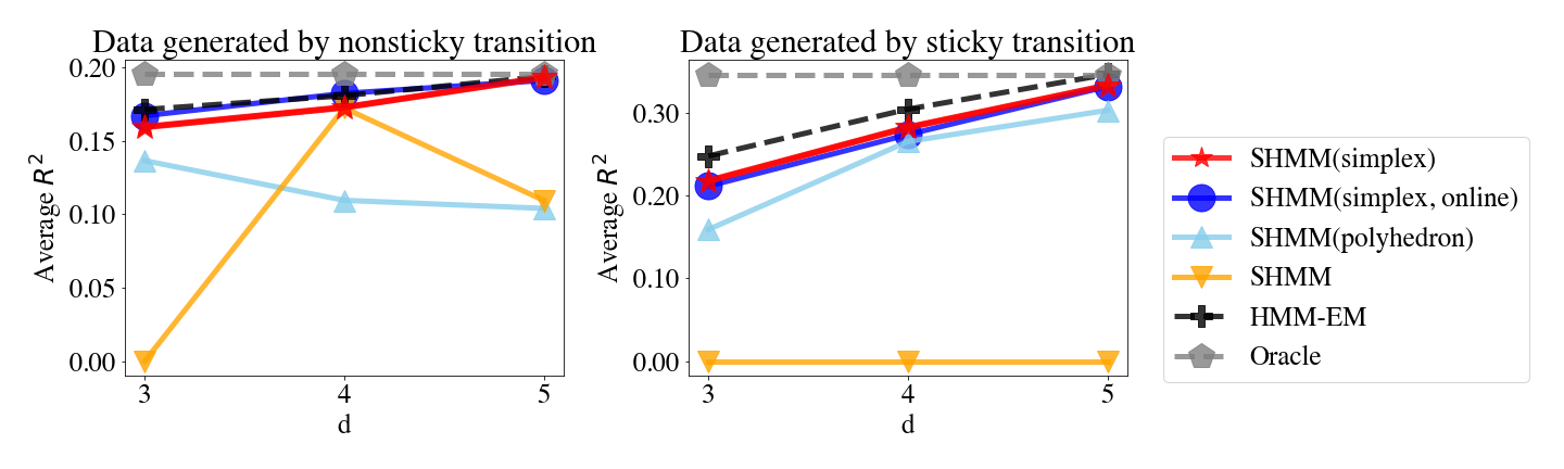
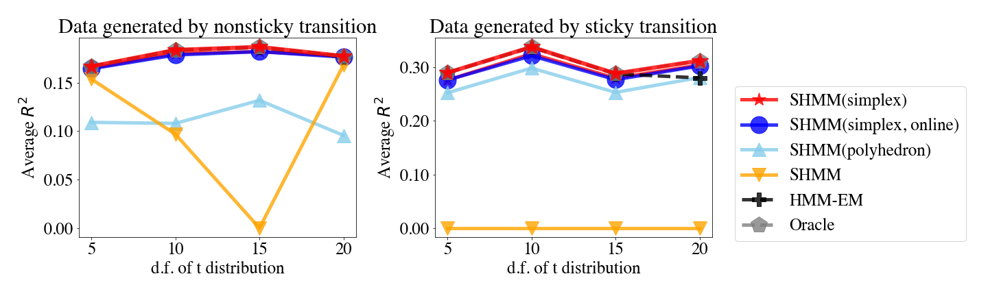
Figure 7: These subfigures show the simulation results for experimental settings in Section 5.1.1. The left column shows the results from sticky transitions, and the right column from nonsticky transitions. The first row examines the effect of $\sigma$ (data generated using a 5-state GHMM), the second row shows the effect of misspecification of the dimensionality $d$ (data generated from a 5-state GHMM with $\sigma=0.05$), and the last row shows the results under non-gaussian emissions (data generated using a 5-state HMM with t-distributed emissions and $\sigma=0.05$, under varying degrees of freedom). In each subfigure, the y-axis is average $R^{2}$. For $R^{2}<0$, we threshold at $0$ for plotting purposes. See supplementary for detailed results.

Figure 7 shows that PSHMM performs comparably to E-M. In most cases they achieve similar $R^{2}$, with PSHMM outperforming E-M algorithm under large noise or heavy-tails. Note that we allow multiple initializations under the E-M algorithm in order to avoid being trapped in local optima. However, this substantially increases the computational time. Finally, we note that dimension of the simulated observed data was set at $dim=100$. In our simulations, we found that this approached the useful limit of the E-M algorithm. When we tried the simulated data with $dim=1000,10000$, the E-M algorithm failed, while SHMM still performed well. Here for comparison, we show the results with data of $dim=100$.

The last point is an important one. In Figure 7, in order to include the E-M algorithm in our simulations, we restrict our investigation to settings where E-M is designed to succeed, and show comparable performance with our methodology. Many real-world scenarios exist in a space where E-M is a non-starter.

In Figure 7, we can also see that adding projections to SHMM greatly improved $R^{2}$, achieving near oracle-level performance in some settings. The top row shows that under both high or low signal-to-noise scenarios, PSHMM works well. The middle row shows that PSHMM is robust and outperforms SHMM when the model is mis-specified, for example, when the underlying data contains 5 states but we choose to reduce the dimensions to $3$ or $4$. The last row shows that PSHMM is more robust and has a better $R^{2}$ than SHMM with heavy-tailed data such as data generated by a t distribution. In all figures, when $R^{2}<0$, we threshold to $0$ for plotting purpose. See supplementary tables for detailed results. Negative $R^{2}$ occurs only for the standard SHMM, and implies that it is not stable. Since we simulated $100$ trials for each setting, in addition to computing the mean $R^{2}$ we could also calculate the variance of the $R^{2}$ metric. We provide the variance of the $R^{2}$ in the appendix, but note here that the variance of $R^{2}$ under PSHMM was smaller than that of the SHMM. Overall, while SHMM often performs well, it is not robust, and PSHMM provides a suitable solution.

Finally, in all simulation settings, we see that the standard SHMM tends to give poor predictions except in non-sticky and high signal-to-noise ratio settings. PSHMM is more robust against noise and mis-specified models. Among the PSHMM variants, projection-onto-simplex outperforms projection-onto-polyhedron. The reason is that the projection-onto-simplex has a dedicated optimization algorithm that guarantees the optimal solution in the projection step. In contrast, projection-onto-polyhedron uses the log-barrier method, which is a general purpose optimization algorithm and does not guarantee the optimality of the solution. Since projection-onto-polyhedron also has a higher computational time, we recommend using projection-onto-simplex. Additionally, for projection-onto-simplex, we see that online and offline estimation perform similarly in most settings, suggesting that online learning does not lose too much power compared with offline learning.

5.2 Testing the effectiveness of forgetfulness

Experimental setting.

Similarly to Section 5.1.1, we simulated 100-dimensional, 5-state GHMM data with $\sigma=\{0.01,0.05,0.1,0.5,1.0\}$ and of length $2000$ where the first $1000$ steps are for training and the last $1000$ steps are for testing. The transition matrix is no longer time-constant but differ in the training and testing period as follows:

• training period (diagonal-0.8): $\bm{T}^{(train)}=[\bm{T}_{ij}^{(train)}]_{i=1,\cdots,5}^{j=1,\cdots,5}=[0.75\times\mathrm{I}\{i=j\}+0.05]_{i=1,\cdots,5}^{j=1,\cdots,5}$;

• testing period (antidiagonal-0.8): $\bm{T}^{(test)}=[\bm{T}_{ij}^{(test)}]_{i=1,\cdots,5}^{j=1,\cdots,5}=[0.75\times\mathrm{I}\{i+j=5\}+0.05]_{i=1,\cdots,5}^{j=1,\cdots,5}$.

We tested different methods on the last 100 time steps, including the standard SHMM, projection-onto-simplex SHMM, online learning projection-onto-simplex SHMM, online learning projection-onto-simplex SHMM with decay factor $\gamma=0.05$, E-M, and the oracle as defined above. For online learning methods, we used the first $100$ steps in the training set for warm-up and incorporated the remaining $900$ samples using online updates.

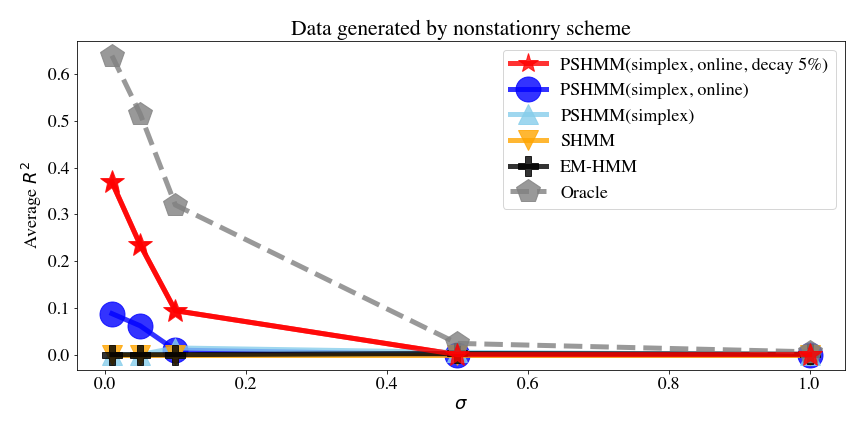
Figure 8: Simulation results for online learning variants. The simulations are generated using a 5-state GHMM across a variety of $\sigma$ settings and time-varying transition distributions. The y-axis is the average $R^{2}$. As before, for $R^{2}<0$, we threshold at $0$ for plotting purposes. See supplementary for detailed results.

Simulation results.

Figure 8 shows the simulation results. Since the underlying data generation process is no longer stationary, most methods failed including the E-M algorithm, with the exception of the online learning projection-onto-simplex SHMM with decay factor $=0.05$. Adding the decay factor was critical for accommodating non-stationarity. PSHMM with decay factor outperformed the other methods since adding forgetfulness helps accommodate the changing patterns. As $\sigma$ increases even PSHMM performs poorly– the oracle shows that this degredation in performance is hard to overcome.

5.3 Testing Computational Time

Experimental setting

We used a similar experimental setting from Section 5.1.1. We simulated 100-dimensional, 3-state GHMM data with $\sigma=0.05$ and length 2000. We used the first half for warm-up and test computational time on the last 1000 time steps. We tested both E-M algorithm and SHMM (all variants). For the SHMM family of algorithms, we tested under both online and offline learning regimes. We computed the total running time in seconds. The implementation is done in python with packages Numpy (Harris et al.,, 2020), Scipy (Virtanen et al.,, 2020) and scikit-learn (Pedregosa et al.,, 2011) without multithreading. Note that in contrast to our previous simulations, the entire process is repeated only 30 times. The computational time is the average over the 30 runs.

Simulation results

Table 2 shows the computational times for each method. First, online learning substantially reduced the computational cost. For the offline learning methods, projection-onto-simplex SHMM performed similarly to SHMM, and projection-onto-polyhedron was much slower. In fact, the offline version of projection-onto-polyhedron was slow even compared to the the E-M algorithm. However, the online learning variant of projection-onto-polyhedron was much faster than the Baum-Welch algorithm. Taking both the computational time and prediction accuracy into consideration, we conclude that online and offline projection-onto-simplex SHMM are the best choices among these methods.

Method	Offline/online	Computational time (sec)
E-M (Baum-Welch)	-	2134
SHMM	offline	304
SHMM	online	0.5
PSHMM (simplex)	offline	521
PSHMM (simplex)	online	0.7
PSHMM (polyhedron)	offline	10178
PSHMM (polyhedron)	online	14

Table 2: Simulation results for comparing computational time among different methods.

6 Application: Backtesting on High Frequency Crypto-Currency Data

6.1 Data Description & Experiment Setting

To show the performance of our algorithm on real data, we used a crypto currency trading records dataset published by Binance (https://data.binance.vision), one of the largest Bitcoin exchanges in the world. We used the minute-level data and used the calculated log returns for each minute as the input for the models. We set aside a test set from 2022-07-01 to 2022-12-31. For each day in the test set, we used a previous 30-day rolling period to train the models, and made consecutive-minute recursive predictions over the testing day without updating the model parameters. For currency, we chose Bitcoin, Ethereum, XRP, Cardano and Polygon. For prediction, we used the HMM with E-M inference (HMM-EM), SHMM, and PSHMM (simplex) and compared their performance. For HMM-EM, SHMM and PSHMM, we chose to use 4 latent states. This was motivated by the fact that there are 4 dominant types of log returns: combinations of large/small gain/loss.

Ultimately, we evaluated models based on the performance of a trading strategy. Translating predictions into a simulated trading strategy is straightforward, and proceeds as follows. If we forecast a positive return in the next minute, we buy the currency, and if we forecast a negative return, we short-sell the currency. We buy a fixed dollar amount of crypto-currency for each of the 5 currencies, hold it for one minute, and then sell it. We repeat this for every minute of the day, and calculate the return of that day as

$$R_{m}=\frac{1}{5}\sum_{i=1}^{5}\sum_{t}sign(\widehat{Y}_{i,t}^{(m)})Y_{i,t}^{(m)}$$

where $Y_{i,t}^{(m)}$ is the return for minute $t$ of day $m$ for currency $i$, $\widehat{Y}_{i,t}^{(m)}$ is its prediction, and $sign(a)$ is $1$ if $a$ is positive, $-1$ if $a$ is negative, and $0$ if $a=0$. Over a period of $M$ days, we obtain $R_{1},\cdots,R_{M}$ and calculate the annualized return,

$$Annualized\ return=365\times\overline{R},$$

the Sharpe ratio (Sharpe,, 1966)

$$Sharpe\ ratio=\frac{\sqrt{365}\times\overline{R}}{\widehat{std}(R)},$$

where $\overline{R}$ and $\widehat{std}(R)$ are the sample mean and standard deviation of the daily returns, and the maximum drawdown (Grossman and Zhou,, 1993)

$$Maximum\ drawdown=\max_{m_{2}}\max_{m_{1}<m_{2}}\left[\frac{\sum_{m=m_{1}}^{m_{2}}(-R_{m})}{1+\sum_{m=1}^{m_{1}}R_{m}}\right].$$

These three metrics are standard mechanisms for evaluating the success of a trading strategy in finance. The annualized return shows the ability of a strategy to generate revenue and is the most straightforward metric. Sharpe ratio is the risk-adjusted return, or the return earned per unit of risk, where the standard deviation of the return is viewed as the risk. In general, we can increase both the return and risk by borrowing money or adding leverage, so Sharpe ratio is a better metric than annualized return because it is not affected by the leverage effect. Maximum drawdown is the maximum percentage of decline from the peak. Since the financial data is leptokurtic, the maximum drawdown shows the outlier effect better than the Sharpe ratio which is purely based on the first and second order moments. A smaller maximum drawdown indicates that the method is less risky.

6.2 Results

Method	Sharpe Ratio	Annualized Return	Maximum drawdown
PSHMM	$2.88$	$1012\%$	$49\%$
SHMM	$1.07$	$345\%$	$90\%$
HMM-EM	$0.89$	$197\%$	$53\%$

Table 3: Real-world application results: PSHMM, SHMM, HMM-EM and AR on crypto-currency trading.

From Table 3, we see that PSHMM outperforms all other benchmarks with the highest Sharpe ratio and annualized return, and the lowest maximum drawdown. PSHMM outperforms SHMM and SHMM outperforms HMM-EM. SHMM outperforms HMM-EM because the spectral learning doesn’t suffer from the local minima problem of E-M algorithm. PSHMM outperforms SHMM because the projection-onto-simplex provides regularization.

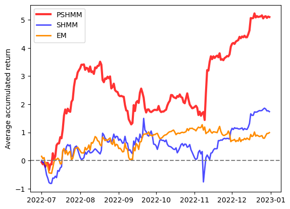
Figure 9: The average accumulated return of crypto currencies.

The accumulated daily return is shown in Figure 9. PSHMM well-outperformed the other methods. The maximum drawdown of PSHMM is $49\%$. Considering the high volatility of the crypto currency market during the second half of 2022, this maximum drawdown is acceptable. For computational purposes, the drawdown is allowed to be larger than $100\%$ because we are always using a fixed amount of money to buy or sell, so effectively we are assuming an infinite pool of cash. Between PSHMM and SHMM, the only difference is from the projection-onto-simplex. We see that the maximum drawdown of PSHMM is only about half that of SHMM, showing that PSHMM takes a relatively small risk, especially given that PSHMM has a much higher return than SHMM. Combining the higher return and lower risk, PSHMM performs substantially better than SHMM.

7 Discussion

Spectral estimation avoids being trapped in local optima.

E-M (i.e. the B-W algorithm) optimizes the likelihood function and is prone to local optima since the likelihood function is highly non-convex, while spectral estimation uses the MOM directly on the observations. Although multiple initializations can mitigate the local optima problem with E-M, it, there is no guarantee that it will convergence to the true global optimum. Spectral estimation provides a framework for estimation which not only avoids non-convex optimization, but also has nice theoretical properties. The approximate error bound tells us that when the number of observations goes to infinity, the approximation error will go to zero. In this manuscript, we also provide the asymptotic distribution for this error.

Projection-onto-simplex serves as regularization.

The standard SHMM can give poor predictions due to the accumulation and propagation of errors. Projection-onto-simplex pulls the prediction back to a reasonable range. This regularization is our primary methodological innovation, and importantly makes the SHMM well-suited for practical use. Although the simplex, estimated by the means from a GMM, can be biased, this simplex provides the most natural and reasonable choice for a projection space. We can think of this as a bias-variance trade-off. When the data size is small, this regularization sacrifices bias to reduce variance.

Online learning can adapt to dynamic patterns and provide faster learning.

Finally, we provide an online learning strategy that allows the estimated moments to adapt over time, which is critical in several applications that can exhibit nonstationarity. Our online learning framework can be applied to both the standard SHMM and PSHMM. Importantly, online learning substantially reduces the computational costs compared to re-training the entire model prior to each new prediction.

SUPPLEMENTAL MATERIALS

Python-package for SHMM and PSHMM:

Python-package $PSHMM$ contains code to perform the SHMM and PSHMM described in the article. The package also contains an illustration of package usage. (.zip file)

Proofs:

Detailed proof for Lemma 1 in Section 2. (.pdf file)

Simulation details:

Detailed simulation results for Figure 7 (.pdf file)

References

- Baum and Petrie, (1966) Baum, L. E. and Petrie, T. (1966). Statistical inference for probabilistic functions of finite state markov chains. The annals of mathematical statistics, 37(6):1554–1563.
- Baum et al., (1970) Baum, L. E., Petrie, T., Soules, G., and Weiss, N. (1970). A maximization technique occurring in the statistical analysis of probabilistic functions of markov chains. The annals of mathematical statistics, 41(1):164–171.
- Boyd et al., (2004) Boyd, S., Boyd, S. P., and Vandenberghe, L. (2004). Convex optimization. Cambridge university press.
- Dempster et al., (1977) Dempster, A. P., Laird, N. M., and Rubin, D. B. (1977). Maximum likelihood from incomplete data via the em algorithm. Journal of the Royal Statistical Society: Series B (Methodological), 39(1):1–22.
- Eckart and Young, (1936) Eckart, C. and Young, G. (1936). The approximation of one matrix by another of lower rank. Psychometrika, 1(3):211–218.
- Fontenla-Romero et al., (2013) Fontenla-Romero, Ó., Guijarro-Berdiñas, B., Martinez-Rego, D., Pérez-Sánchez, B., and Peteiro-Barral, D. (2013). Online machine learning. In Efficiency and Scalability Methods for Computational Intellect, pages 27–54. IGI global.
- Frisch, (1955) Frisch, K. (1955). The logarithmic potential method of convex programming. Memorandum, University Institute of Economics, Oslo, 5(6).
- Grossman and Zhou, (1993) Grossman, S. J. and Zhou, Z. (1993). Optimal investment strategies for controlling drawdowns. Mathematical finance, 3(3):241–276.
- Halko et al., (2011) Halko, N., Martinsson, P.-G., and Tropp, J. A. (2011). Finding structure with randomness: Probabilistic algorithms for constructing approximate matrix decompositions. SIAM review, 53(2):217–288.
- Harris et al., (2020) Harris, C. R., Millman, K. J., van der Walt, S. J., Gommers, R., Virtanen, P., Cournapeau, D., Wieser, E., Taylor, J., Berg, S., Smith, N. J., Kern, R., Picus, M., Hoyer, S., van Kerkwijk, M. H., Brett, M., Haldane, A., del Río, J. F., Wiebe, M., Peterson, P., Gérard-Marchant, P., Sheppard, K., Reddy, T., Weckesser, W., Abbasi, H., Gohlke, C., and Oliphant, T. E. (2020). Array programming with NumPy. Nature, 585(7825):357–362.
- Hsu et al., (2012) Hsu, D., Kakade, S. M., and Zhang, T. (2012). A spectral algorithm for learning hidden markov models. Journal of Computer and System Sciences, 78(5):1460–1480.
- Knoll et al., (2016) Knoll, B. C., Melton, G. B., Liu, H., Xu, H., and Pakhomov, S. V. (2016). Using synthetic clinical data to train an hmm-based pos tagger. In 2016 IEEE-EMBS International Conference on Biomedical and Health Informatics (BHI), pages 252–255. IEEE.
- Lahmiri and Bekiros, (2021) Lahmiri, S. and Bekiros, S. (2021). Deep learning forecasting in cryptocurrency high-frequency trading. Cognitive Computation, 13:485–487.
- McLachlan and Basford, (1988) McLachlan, G. J. and Basford, K. E. (1988). Mixture models: Inference and applications to clustering, volume 38. M. Dekker New York.
- Pedregosa et al., (2011) Pedregosa, F., Varoquaux, G., Gramfort, A., Michel, V., Thirion, B., Grisel, O., Blondel, M., Prettenhofer, P., Weiss, R., Dubourg, V., Vanderplas, J., Passos, A., Cournapeau, D., Brucher, M., Perrot, M., and Duchesnay, E. (2011). Scikit-learn: Machine learning in Python. Journal of Machine Learning Research, 12:2825–2830.
- Rodu, (2014) Rodu, J. (2014). Spectral estimation of hidden Markov models. University of Pennsylvania.
- Rodu et al., (2013) Rodu, J., Foster, D. P., Wu, W., and Ungar, L. H. (2013). Using regression for spectral estimation of hmms. In International Conference on Statistical Language and Speech Processing, pages 212–223. Springer.
- Sharpe, (1966) Sharpe, W. F. (1966). Mutual fund performance. The Journal of business, 39(1):119–138.
- Song et al., (2010) Song, L., Boots, B., Siddiqi, S. M., Gordon, G., and Smola, A. (2010). Hilbert space embeddings of hidden markov models. In Proceedings of the 27th International Conference on International Conference on Machine Learning, ICML’10, page 991–998, Madison, WI, USA. Omnipress.
- Virtanen et al., (2020) Virtanen, P., Gommers, R., Oliphant, T. E., Haberland, M., Reddy, T., Cournapeau, D., Burovski, E., Peterson, P., Weckesser, W., Bright, J., van der Walt, S. J., Brett, M., Wilson, J., Millman, K. J., Mayorov, N., Nelson, A. R. J., Jones, E., Kern, R., Larson, E., Carey, C. J., Polat, İ., Feng, Y., Moore, E. W., VanderPlas, J., Laxalde, D., Perktold, J., Cimrman, R., Henriksen, I., Quintero, E. A., Harris, C. R., Archibald, A. M., Ribeiro, A. H., Pedregosa, F., van Mulbregt, P., and SciPy 1.0 Contributors (2020). SciPy 1.0: Fundamental Algorithms for Scientific Computing in Python. Nature Methods, 17:261–272.
- Wang and Carreira-Perpinán, (2013) Wang, W. and Carreira-Perpinán, M. A. (2013). Projection onto the probability simplex: An efficient algorithm with a simple proof, and an application. arXiv preprint arXiv:1309.1541.