Spatially heterogeneous learning by a deep student machine

Hajime Yoshino Cybermedia Center, Osaka University, Toyonaka, Osaka 560-0043, Japan Graduate School of Science, Osaka University, Toyonaka, Osaka 560-0043, Japan
Abstract

Despite the spectacular successes, deep neural networks (DNN) with a huge number of adjustable parameters remain largely black boxes. To shed light on the hidden layers of DNN, we study supervised learning by a DNN of width $N$ and depth $L$ consisting of $NL$ perceptrons with $c$ inputs by a statistical mechanics approach called the teacher-student setting. We consider an ensemble of student machines that exactly reproduce $M$ sets of $N$ dimensional input/output relations provided by a teacher machine. We show that the statistical mechanics problem becomes exactly solvable in a high dimensional limit which we call as ’dense limit’: $N\gg c\gg 1$ and $M\gg 1$ with fixed $\alpha=M/c$ using the replica method developed in (Hajime Yoshino, SciPost Phys. Core 2, 005 (2020)) Yoshino (2020). In parallel to the theoretical study, we also study the model numerically performing simple greedy Monte Carlo simulations. Simulations reveal that learning by the DNN is quite heterogeneous in the network space: configurations of the teacher and the student machines are more correlated within the layers closer to the input/output boundaries while the central region remains much less correlated due to the over-parametrization in qualitative agreement with the theoretical prediction. We evaluate the generalization-error of the DNN with various depth $L$ both theoretically and numerically. Remarkably both the theory and simulation suggest generalization-ability of the student machines, which are only weakly correlated with the teacher in the center, does not vanish even in the deep limit $L\gg 1$ where the system becomes heavily over-parametrized. We also consider the impact of effective dimension $D(\leq N)$ of data by incorporating the hidden manifold model (Sebastian Goldt, Marc Mézard, Florent Krzakala, and Lenka Zdevorová, Physical Review X 10, 041044 (2020). Goldt et al. (2020)) into our model. The replica theory implies that the loop corrections to the dense limit, which reflect correlations between different nodes in the network, become enhanced by either decreasing the width $N$ or decreasing the effective dimension $D$ of the data. Simulation suggests both leads to significant improvements in generalization-ability.

I Introduction

The mechanism of machine learning by deep neural networks (DNN) LeCun et al. (2015) remains largely unknown. One of the most puzzling points is the issue of over-parametrization: supervised learning by DNN can work even in the regime where the number of adjustable parameters is larger than the data size by orders of magnitudes. This goes sharply against the traditional wisdom of data modeling: for example, one should avoid fitting $10$ data points by a fitting function with $100$ adjustable parameters, which is just nonsense. However empirically it has been found repeatedly that such over-parametrized DNNs can somehow avoid over-fitting and generalize well, i. e. they can successfully describe new data not used during training. Uncovering the reason for this peculiar phenomenon is a very interesting and challenging scientific problem Carleo et al. (2019); Geiger et al. (2020). An important point to be noted is that the effective dimension $D$ of the data which can be much smaller than the apparent dimension $N$ of data. It has been shown in studies of shallow networks that the generalization ability improves by increasing $N/D$ due to a kind of self-averaging mechanism Mei and Montanari (2022); Loureiro et al. (2022); d’Ascoli et al. (2021). However, the generalization ability of the deeper system remains unexplained.

Statistical mechanics on neural networks has a long history that dates back to the 1980’s Amit et al. (1985); Gardner (1988); Gardner and Derrida (1989). Studies on the single perceptrons Gardner (1988); Gardner and Derrida (1989) and shallow networks Mei and Montanari (2022); Gerace et al. (2020) have provided many useful insights and some progresses have been made also on deeper networks Gabrié et al. (2018); Aubin et al. (2019); Schröder et al. (2023); Cui et al. (2023). However what is going on in the hidden layers remain largely unknown. The first attempt to uncover the black box was made in Yoshino (2020) by the present author based on the replica method and predicted unexpected phenomenology of DNN: spatially heterogeneous learning. Unfortunately the theory suffered a serious problem due to an uncontrolled approximation and the validity of the prediction remained elusive.

Refer to caption
Figure 1: Schematic picture of the multi-layer perceptron network of depth $L$ and width $N$. In this example, the depth is $L=4$. Each arrow represents a $M$-component vector spin ${\bf S}_{i}=(S_{i}^{1},S_{i}^{2},\ldots,S_{i}^{M})$ with its component $S_{i}^{\mu}=\pm 1$ representing the state of a ’neuron’ in the $\mu$-th pattern.

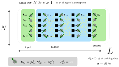
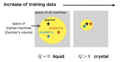
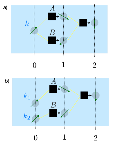
To understand the mechanism for the generalization ability of deep networks, we study supervised learning by DNN considering the so-called teacher-student setting which is a canonical setting to study statistical inference problems Engel and Van den Broeck (2001); Zdeborová and Krzakala (2016) by methods of statistical mechanics. We consider a prototypical DNN of rectangular shape with width $N$ and depth $L$ consisting of $NL$ perceptrons with $c$ inputs, which defines a mapping between a $N$ dimensional input vector to a $N$ dimensional output vector (See Fig. 1). For the data, we consider $M$ pairs of input/output vectors provided by a teacher machine and we consider an ensemble of student machines that exactly satisfy the same input/output relations as the teacher. The phase space volume of such an ensemble is called as Gardner’s volume Gardner (1988); Gardner and Derrida (1989) which should be very large for over-parametrized DNNs. In fact, it is known that gradient descent dynamics find such a machine without going over barriers in the loss landscape Jacot et al. (2018); Mei et al. (2018); Chizat and Bach (2018). In Fig. 2, we show a schematic picture of the phase space of the machines. If $M$ is small, typically students will not find the teacher. This situation would be regarded as liquid phase. If $M$ is increased, crystalline phase may emerge in which students find the (hidden) crystal, i. e. teacher. We also wish consider the impact of effective dimension $D$ of the data by incorporating the hidden manifold model Goldt et al. (2020); Gerace et al. (2020); Goldt et al. (2022)) in our model. Using methods of statistical mechanics we wish to investigate how different machines which satisfy the same set of input/output boundary conditions become correlated with each other in the hidden layers and evaluate their generalization ability : the ability of the students to reproduce the teacher’s output against new input data not used in training.

Refer to caption
Figure 2: Schematic picture of the phase space of machines: the gray box represents the set of all machines which can be generated varying the parameters (e.g. synaptic weights) given a network structure. The yellow region resents the subspace in which machines agree teacher’s machine for a given $M$ set of training data. Liquid phase: if the number of the training data $M$ is small, the subspace is so large that the machines are typically widely separated and their mutual overlap $Q$ is typically zero . Crystalline phase: $M$ is large enough, that machines have finite overlap $Q$ with respect to each other.

The first attempt to tackle the statistical mechanics problem of DNN was made recently in Yoshino (2020) based on the replica method in a high dimensional limit with $c=N=D\gg 1$ and $M\gg 1$ with fixed $\alpha=M/c$. Unfortunately it suffered from an uncontrolled ’tree’ approximation which is invalid for the global coupling case $c=N$. In the present paper we show that the problem can be overcome in the limit $N\gg c\gg 1$, which we call as dense limit. As the result we establish an exactly solvable statistical mechanics model of DNN which has been waited for a long time.

Using the exact solution of the model which can be obtained by the replica method developed in Yoshino (2020), we analyze the key question: generalization-ability of DNN including the over-parametrized regime. We also show that the effect of the finiteness of the width (apparent dimension of the data) $N$ and the effective dimension $D$ similarly enhances loop corrections which induce correlations between distant layers. In parallel to the theoretical study, we also perform extensive numerical simulations to examine the theoretical predictions. We use the Monte Carlo method which allows more efficient exploration of the solution space compared with the usual gradient descent algorithms.

The following sections are organized as follows. In sec II we summarize the main results of this paper. In sec III we introduce our model. We discuss the replica approach in sec IV and numerical simulations in sec V. In sec VI we conclude this paper with perspectives. In appendix A we discuss a connection between some layered spinglass models and DNNs and in appendix B we present some details of the replica theory.

II Summary of results

Let us summarize below the main results of this work. On the theoretical side we find the following.

  • We establish an exactly solvable statistical mechanics model of DNN in the dense Limit $N\gg c\gg 1$. The exact solution of the model is obtained using replica the approach. It is shown that the correction to the dense limit due to finiteness of the width $N$ can be expressed by loop-corrections. Fortunately, it turns out that the theoretical results presented in Yoshino (2020) are essentially valid in the dense limit $N\gg c\gg 1$ although they are unjustified for the global coupling $c=N$ assumed there.

  • We show that smallness of the effective dimension $D(<N)$ of the hidden manifold model Goldt et al. (2020) enhances the loop corrections. Thus finite dimension $D$ effect is predicted to be similar to finite width $N$ effect.

  • The learning curve $\epsilon=\epsilon_{L}(\alpha)$ of the DNN with various depth $L$ is analyzed evaluating the generalization error $\epsilon_{L}(\alpha)$ in the case of Bayes optimal teacher-student setting where the replica symmetry holds. It becomes independent of the depth $L$, i. e. $\epsilon_{L}(\alpha)=\epsilon_{\infty}(\alpha)$ as long as the network is deep enough such that liquid phase, where students are de-correlated from the teacher, remain in the center reflecting strong over-parametrization.

On the numerical side we find the following.

  • We simulated the model with finite connectivity $c$ and width $N$ in the Bayes-optimal teacher-student setting and found that a simple greedy Monte Carlo algorithm allows the student machines to equilibrated after sufficiently long times. Thus typical equilibrium states are accessible starting from typical random initial configurations without going over barriers in the loss landscape.

  • Observation of the overlap between the machines reveal spatially in-homogeneous learning in qualitative agreement with the theory. While the theory in the dense limit $N\gg c\gg 1$ predicts, in the case of strong over-parametrization, crystalline regions with finite overlap close to the input/output layers separated by a liquid region with zero overlap in the center, the distinction between the crystalline and the liquid phases become blurred in systems with finite width $N$ and finite connectivity $c$. Nonetheless, the presence of the liquid like region in the center becomes clearer by making the width $N$ large and the connectivity $c$ large or the depth $L$ large. We consider that the remnant overlap left in the center by the finite width $N$ and finite connectivity $c$ effects play the role of symmetry breaking field which connect the two crystalline regions attached to the boundaries.

  • Observation of the learning curve $\epsilon=\epsilon_{L,c,N,D}(\alpha)$ reveal that it becomes independent of the depth $L$ in deep enough systems in agreement with the theoretical prediction.

  • The observation reveal that finite effective dimension $D$ effect and finite width $N$ effects are indeed very similar as suggested by the consideration of the loop effects in the theory. The generalization error $\epsilon_{L,c,N,D}(\alpha)$ decreases significantly decreasing either the width $N$ or the effective dimension $D$.

III Model

III.1 Multi-layer perceptron network

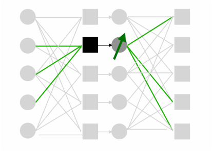
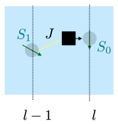
We consider a simple multi-layer neural network of a rectangular shape with width $N$ and depth $L$ (see Fig. 1). The input and output layers are located at the boundaries $l=0$ and $L$ respectively while $l=1,2,\ldots,L-1$ are hidden layers. On each layer $l=0,1,2,\ldots,L$ there are $N$ neurons labeled as $(l,i)$ with $i=1,2,\ldots,N$. The state of the neuron $(l,i)$ is represented by an Ising spin $S_{l,i}$: it is active if $S_{l,i}=1$ and inactive if $S_{l,i}=-1$.

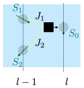
The network is constructed as follows. There are $N_{\blacksquare}=NL$ perceptrons. Consider a perceptron $\blacksquare=(l,i)$ which is the $i$-th neuron in the $l$-th layer. It receives $c$ inputs from the outputs of the perceptrons $\blacksquare(k)$ $(k=1,2,\ldots,c)$ in the previous $l-1$-th layer, weighted by ${\bf J}_{\blacksquare}=(J_{\blacksquare}^{1},J_{\blacksquare}^{2},\ldots,J_{\blacksquare}^{c})$. (For the special case $l=1$, $\blacksquare(k)$ should be understood as one of the spins in the input layer.) The $c$ perceptrons are selected randomly out of $N$ possible perceptrons in the $l-1$ th layer.

The output of the perceptron $\blacksquare$, which we denote as $S_{\blacksquare}$, is given by,

$$S_{\blacksquare}={\rm sgn}\left(\frac{1}{\sqrt{c}}\sum_{k=1}^{c}J_{\blacksquare}^{k}S_{\blacksquare(k)}\right)$$ (1)

where ${\rm sgn}(y)=y/|y|$ is our choice for the activation function. We assume that the synaptic weights $J^{k}_{\blacksquare}$ take real numbers normalized such that,

$$\sum_{k=1}^{c}(J^{k}_{\blacksquare})^{2}=c.$$ (2)

For convenience, we call the state of the neurons $S_{l,i}$’s as ’spins’, and the synaptic weights $J_{\blacksquare}^{k}$s as ’bonds’ in the present paper. We denote the set of perceptrons in the $l$-th layer as $\blacksquare\in l$ and denote the set of perceptrons whose outputs become input for $\blacksquare$ as $\partial\blacksquare$, i. e. $\partial\blacksquare=\{\blacksquare(1),\blacksquare(2),\ldots,\blacksquare(c)\}$. For convenience we introduce also $\blacksquare\in 0$ so that we can write the set of spins in the input layer as $S_{\blacksquare\in 0}$.

III.2 Dense coupling

As stated above, $c$ legs of a perceptron $\blacksquare$ at $l$-th layer is connected to $c$ neurons $S_{\blacksquare(k)}$ $(k=1,2,\ldots,c)$ in the previous $l-1$-th layer. The $c$ neurons out of $N$ possible neurons are selected randomly. Thus our graph becomes a sort of sparse (layered) random graph when $c$ is finite. We will find in sec. IV that this construction enables us to obtain an exactly solvable statistical mechanics model of DNN because of the following reasons.

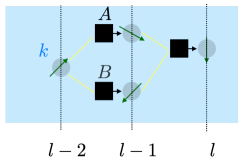
  • The graph becomes locally tree-like as in the case of Bethe-lattices so that contributions of ’loops’ can be neglected in the wide limit $N\rightarrow\infty$ with fixed $c$. This can be seen as follows. For instance, consider a loop $0\rightarrow 1\rightarrow 2\rightarrow 3\rightarrow 0$ shown in Fig. 3. Starting from 00, choose any $1$ connected to 00. Then choose any $2$ connected to $1$. Then choose any $3$ (different from $1$) connected to 00. In the case of global coupling $c=N$, $2$ is certainly connected to $3$ completing a loop. However, in the case of dense coupling, in a given realization of the random graph, $2$ is connected to $3$ only with a probability $\sim c/N$. Thus in the limit $N\rightarrow\infty$ with fixed $c$, the probability to complete the loop vanishes. This argument can be generalized for 2-loops, 3-loops,….which happen with probability $O(c/N)^{2})$, $O(c/N)^{3})$, … Note that the loops cannot be neglected. In the case of global coupling $c=N$ (assumed in Yoshino (2020)).

    Refer to caption
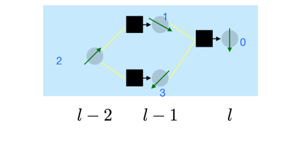
    Figure 3: A loop of interactions in a DNN extended over 3 layers, through 3 perceptrons and 4 bonds.
  • In the case of the global coupling $c=N$, the system is symmetric under permutations of the perceptrons within each layer so that one has to consider whether this symmetry becomes broken spontaneously Barkai et al. (1992). In the case of sparse coupling $c<N$, we can eliminate this symmetry by choosing the connections in stochastic ways, i. e. random graph.

  • In the setup of our theory, we finally consider $c\rightarrow\infty$ (and $M=\alpha c\rightarrow\infty$ (see Eq. (5)) (after $N\rightarrow\infty$). This greatly simplifies the theory as it allows us to use the saddle point method in theoretical analysis. We call such intermediately dense coupling with

    $$N\gg c\gg 1$$ (3)

    as dense coupling.

III.3 Connection to spinglasses

The feed-forward network made of perceptrons is equivalent to the zero-temperature limit of the transfer-matrix of a spin-glass with Hamiltonian,

$$H=-\frac{1}{\sqrt{c}}\sum_{\blacksquare}\sum_{k=1}^{c}J_{\blacksquare}^{k}S_{\blacksquare}S_{\blacksquare(k)}$$ (4)

as shown in appendix A. This is a spin-glass model put in a layered structure. Specifying the spin configuration on the boundary $l=0$, spin configurations at layers $l=1,2,\ldots,L$ become specified deterministically in the $T\rightarrow 0$ limit of the transfer matrix. The perceptrons Eq. (1) just do this operation.

An important point is that there are no direct interactions within each layer much as the restricted Boltzmann machines (RBMs)Ackley et al. (1985) which make the operations of the $T=0$ transfer matrices equivalent to the simple feed-forward non-linear mappings Eq. (1). In appendix A we also show that such representations are possible for generic activation functions including the function ${\rm sgn}(y)$ which we employ in this paper just as a special case.

For a given set of interactions $J_{\blacksquare}^{k}$, the ground state of the system is unique if the boundaries are allowed to relax. But here we are considering ground states with different realizations of frozen boundaries. Specifying the boundary condition on one side, the configurations on the other side becomes fixed deterministically.

From this view point, the exponential expressibility of DNN Poole et al. (2016) can be traced back to the chaotic sensitivity of spinglass ground state Bray and Moore (1987); Newman and Stein (1992). Even if a change of the configuration on the boundary $S_{\blacksquare\in 0}^{\mu}\rightarrow S_{\blacksquare\in 0}^{\nu(\neq\mu)}$ is small, the resultant changes of the spin configurations become larger going deeper into the system $l=1,2,\ldots$. This can be viewed as an avalanche process. In deeper layers $l=1,2,\ldots$ larger number of nodes $i=1,2,\ldots$ will be involved in a single avalanche event. In sec. V.2.4 we discuss a quantity which reflects the avalanche sizes, i. e. the number of nodes involved in a same avalanche caused by $S_{\blacksquare\in 0}^{\mu}\rightarrow S_{\blacksquare\in 0}^{\nu(\neq\mu)}$.

III.4 Teacher-Student setting

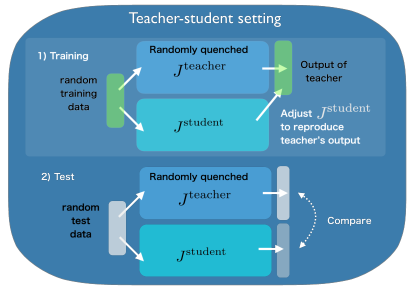
As shown in Fig. 4 we consider a learning scenario by a teacher machine and a student machine. For simplicity we assume that the teacher is a ’quenched-random teacher’: its synaptic weights $\{(J_{\blacksquare}^{k}\}_{\rm teacher}\}$ are iid random variables which take continuous values subjected to the normalization condition Eq. (2).

Training: we generate $M$ sets of training data labeled as $\mu=1,2,\ldots,M$ as follows. The values of the spins in the input layer $S_{\blacksquare\in 0}^{\mu}=\{S^{\mu}_{0,1}\}_{\rm teacher}$ are set as iid random Ising numbers $\pm 1$ ($i=1,2,\ldots,N$, $\mu=1,2,\ldots,M$) and the corresponding output of the teacher $\{S^{\mu}_{L,i}\}_{\rm teacher}$ are obtained. The student does training by adjusting its own synaptic weights $\{(J_{\blacksquare}^{k})_{\rm student}\}$ such that it reproduces perfectly the $M$ sets of the input-output relations of the teacher. More precisely we consider an idealized setting that 1) the student has exactly the same architecture as the teacher including the specific realization of the random network between adjacent layers 2) student knows exactly the $M$ sets of the input/output relations of the teacher. In short, the student knows everything about the teacher except for its actual values of $\{(J_{\blacksquare}^{k})_{\rm teacher}\}$. Within the framework of Bayesian inference, this is a so-called Bayes optimal setting Iba (1999); Zdeborová and Krzakala (2016).

Refer to caption
Figure 4: Schematic pictures of the teacher-student setting.

The configurations of the spins associated with the $M$-patterns of the training data may be represented by $M$-component vectors ${\bf S}_{l,i}=(S_{l,i}^{1},S_{l,i}^{2},\ldots,S_{l,i}^{M})$ (see Fig. 1). In the theory, we will consider $M\rightarrow\infty$ limit with,

$$\alpha\equiv\frac{M}{c}.$$ (5)

fixed. Note that our network is parametrized by $NcL$ variational bonds and the $NM$ constrained spin components on the input and output boundaries. The ratio of the two scales as,

$$r\equiv\frac{NcL}{NM}=\frac{L}{\alpha}$$ (6)

Test (validation): the generalization ability of the student can be examined empirically using a set of test data. Preparing $M^{\prime}$ sets test data as new iid random data $(S^{\mu}_{0,i})_{\rm teacher}$ ($i=1,2,\ldots,N$, $\mu=1,2,\ldots,M^{\prime}$) (not used for the training) we compare the output of the teacher and student machines. The probability that the student makes an error can be measured as,

$$\epsilon=\frac{1}{2}\left(1-\frac{1}{NM^{\prime}}\sum_{\mu=1}^{M^{\prime}}\sum_{i=1}^{N}(S^{\mu}_{L,i})_{\rm teacher}(S^{\mu}_{L,i})_{\rm student}\right).$$ (7)

If the student is just making random guesses $\epsilon=1/2$ while $\epsilon=0$ if it perfectly reproduces the teacher’s output.

III.5 Gardner’s volume

Following the pioneering work by Gardner Gardner (1988); Gardner and Derrida (1989) we investigate the ensemble of all possible machines (choices of the synaptic weights $J_{\blacksquare}^{k}$s) of the student which are perfectly compatible with the $M$ set of the input ${\bf S}_{0}$ and output data ${\bf S}_{L}$ provided by the teacher machine (See Fig. 2). As we noted in sec. III.3, each machine with the feed-forward propagation of signals can be viewed as a zero-temperature limit of the transfer-matrix of a spin-glass with a set of $J_{\blacksquare}^{k}$s. So the ensemble of machines is an ensemble of such transfer matrices, which are typically chaotic.

The phase space volume, which is called Gardner’s volume, can be expressed for the present DNN asYoshino (2020),

$\displaystyle V_{M}\left({\bf S}_{0},{\bf S}_{L}\right)=e^{NM{\cal S}\left({\bf S}_{0},{\bf S}_{l}\right)}$ (8)
$\displaystyle=$ $\displaystyle\left(\prod_{\blacksquare}{\rm Tr}_{{\bf J}_{\blacksquare}}\right)\left(\prod_{\blacksquare\backslash{\rm output}}{\rm Tr}_{{\bf S}_{\blacksquare}}\right)\prod_{\mu=1}^{M}\prod_{\blacksquare}e^{-\beta v(r^{\mu}_{\blacksquare})}\qquad$

where $v(r)$ is a hardcore potential,

$$e^{-\beta v(r)}=\theta(r)$$ (9)

with $\theta(r)$ being the Heviside step function and we introduced the ’gap’ variable,

$$r^{\mu}_{\blacksquare}\equiv S^{\mu}_{\blacksquare}\sum_{k=1}^{c}\frac{J_{\blacksquare}^{k}}{\sqrt{c}}S^{\mu}_{\blacksquare(k)}$$ (10)

The trace over the spin and bond configurations can be written explicitly as,

$${\rm Tr}_{\bf S}=\prod_{\mu=1}^{M}\sum_{S^{\mu}=\pm 1}\qquad{\rm Tr}_{\bf J}=\int_{-\infty}^{\infty}\prod_{j=1}^{c}dJ^{j}\delta\left(\sum_{k=1}^{c}(J^{k})^{2}-c\right)$$ (11)

The key idea behind the expression Eq. (8) is the internal representation Monasson and Zecchina (1995): we are considering the spins (neurons) in hidden layers ($l=1,2,\ldots,L-1$) as dynamical variables in addition to the synaptic weights. This is allowed because the input-output relation of the perceptrons Eq. (1) is forced to be satisfied by requiring the gap to be positive $r_{\mu}^{\blacksquare}>0$ for all perceptrons $\blacksquare=1,2,\ldots,N$ in the network for all training data $\mu=1,2,\ldots,M$ in Eq. (8). As shown in appendix A, the expression Eq. (8) can be also obtained considering the transfer matrix representation.

The main quantity of our interest in the present paper is the generalization error $\epsilon$ Eq. (7). The Gardner’s volume $V_{M}$ provides a way to estimate the generalization ability of the network for the test data Levin et al. (1990); Opper and Kinzel (1996). The probability that the network which perfectly satisfies the constraint put by $M$ sets of training data happens to be compatible with one more unseen data is given by the ratio $V_{M+1}/V_{M}$. Then the generalization error, namely the error probability $\epsilon$, the probability that the configuration of one spin in the output layer $l=L$ of the student machine is wrong (different from the teacher) for a test data can be expressed as,

$$\epsilon=1-\left(\frac{V_{M+1}}{V_{M}}\right)^{1/N}$$ (12)

III.6 Symmetries

Let us note here that there are some symmetries (besides the replica symmetry which we discuss later) in the present problem. The following becomes important, especially in numerical simulations.

III.6.1 Gauge symmetry

Refer to caption
Figure 5: Variables associated with a perceptron $\blacksquare$ which changes sign by the flip of the gauge variable $\sigma_{\blacksquare}\rightarrow-\sigma_{\blacksquare}$

For any $\blacksquare$, the system is invariant under gauge transformation

$\displaystyle S_{\blacksquare}^{\mu}$ $\displaystyle\rightarrow$ $\displaystyle\sigma_{\blacksquare}S_{\blacksquare}^{\mu}\qquad\mu=1,2,\ldots,M$ (13)
$\displaystyle J_{\blacksquare}^{k}$ $\displaystyle\rightarrow$ $\displaystyle\sigma_{\blacksquare}J_{\blacksquare}^{k}\sigma_{\blacksquare(k)}\qquad k=1,2,\ldots,c$ (14)

specified by gauge variables

$$\sigma_{\blacksquare}=\pm 1\qquad\blacksquare=1,2,\ldots,N(L-1)$$ (15)

Note that we do not have a gauge transformation in the output layer $l=L$ since the output layer is constrained. It can be easily seen that the gap variables $r_{\blacksquare}^{\mu}$ (see Eq. (10)) are invariant under the gauge transformation.

Thus for a given realization of a machine with a set of synaptic weights, there are $2^{(L-1)N}$ completely equivalent machines specified by $2^{(L-1)N}$ possible realizations of the gauge variables: all of them operate exactly in the same way yielding the same output for any input. If the synaptic weights only take Ising values $J_{\blacksquare}^{k}=\pm 1$, the number of possible configurations of the machines modulo the gauge symmetry is $2^{NLc^{2}-N(L-1)}$.

The presence of the gauge invariance is natural given the connection to the spinglass as mentioned in sec. III.3. While the gauge variables are frozen in spin-glass problems with quenched bonds Nishimori (2001), here the bonds are dynamical variables so that the gauge variables also evolve in time during learning.

Importantly this is a local symmetry in the sense that change of any $\sigma_{\blacksquare}$ induce changes only in the neighborhood of $\blacksquare$ (see Fig. 5): $S_{\blacksquare}^{\mu}\rightarrow-S_{\blacksquare}^{\mu}$ for $\forall\mu$, $J_{\blacksquare}^{k}\rightarrow-J_{\blacksquare}^{k}$ for $\forall k$, $J_{\square}^{l}\rightarrow-J_{\square}^{l}$ for $\forall(\square,l)$ such that $\square(l)=\blacksquare$. This means that in sparse systems with finite connectivity $c$ and $M(=\alpha c)$, the evolution of the machine from one to another connected by a local gauge transformation takes only a finite time in dynamics. Only in the limit $c\rightarrow\infty$, do such gauge transformations become frozen in time.

III.6.2 Permutation symmetry in globally coupled systems

As we already noted in sec. III.2, in globally coupled systems with $c=N$, the system is invariant under permutations of perceptrons $\blacksquare\in l$ within each layer $l=1,2,\ldots,L$. This symmetry can be removed if the coupling is not global $c<N$ since we can construct random networks (see sec. III.2).

III.7 Hidden manifold

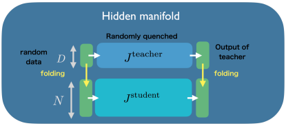
We incorporate the hidden manifold model for the data (S. Goldt et al (2020) Goldt et al. (2020) in our model as the following. We replace the original teacher machine of width $N$ with a narrower teacher machine of with $D(\leq N)$ (see Fig. 6). The teacher is working entirely in $D$ dimensional space being subjected to $D$ dimensional input data and produces $D$ dimensional output. Student machines are provided $N$ dimensional input/output data which are obtained from the $D$ dimensional input/output of the teacher via folding matrices $F_{i,k}$ of size $N\times D$,

$\displaystyle(S_{\rm student})^{\mu}_{0,i}={\rm sgn}\left(\sum_{k=1}^{D}F_{i,k}(S_{\rm teacher})^{\mu}_{0,k}\right)$
$\displaystyle(S_{\rm student})^{\mu}_{L,i}={\rm sgn}\left(\sum_{k=1}^{D}F_{i,k}(S_{\rm teacher})^{\mu}_{L,k}\right)$ (16)

for $i=1,2,\ldots,N$ and $\mu=1,2,\ldots,M$. For the folding matrix, we consider a simple model,

$$F_{i,k}=\left\{\begin{array}[]{ll}1&k={\rm mod}(i-1,D)+1\\ 0&\mbox{otherwise}\end{array}\right.$$ (17)

In this model $N$ elements of the data for students are created simply by making $N/D$ copies of the $D$ elements of the teacher’s data.

Refer to caption
Figure 6: Schematic picture of the hidden manifold model.

IV Replica theory

Now we develop and analyze a replica theory for the statistical mechanics problem of DNN in the dense limit $N\gg c\gg 1$ introduced in sec. III.2. We first show that it can be solved exactly overcoming the issue of uncontrolled approximation made in Yoshino (2020). This is the first main result of this paper. For clarity we repeat the steps made in Yoshino (2020) and indicate how the problem is resolved. Then we revisit the replica symmetric solution in the teacher-student setting presented in Yoshino (2020) and analyze it in more details. Using the exact solution we analyze the generalization-ability of DNN evaluating the generalization error $\epsilon$ via Eq. (12), which is second main result of this paper. The technical details of the theory is presented in appendix  B.

IV.1 Formalism

IV.1.1 Order parameters

We are considering the dense coupling Eq. (3) in which 1) perceptrons have large connectivity $c\gg 1$ and 2) the permutation symmetry of the perceptrons which exist in globally coupled systems is removed. We are also considering a large number of training patterns $M=\alpha c\gg 1$ (see Eq. (5)). Then we can naturally introduce ’local’ order parameters associated with each perceptron $\blacksquare$,

$$Q_{ab,\blacksquare}=\frac{1}{c}\sum_{k=1}^{c}(J_{\blacksquare}^{k})^{a}(J_{\blacksquare}^{k})^{b}\qquad q_{ab,\blacksquare}=\frac{1}{M}\sum_{\mu=1}^{M}(S_{\blacksquare}^{\mu})^{a}(S_{\blacksquare}^{\mu})^{b}$$ (18)

The overlaps between the teacher and student machines are represented by $Q_{0b,\blacksquare}=Q_{b0,\blacksquare}$ and $q_{0b,\blacksquare}=q_{b0,\blacksquare}$ ($b=1,2,\ldots,s$) while those between the student machines are are represented by $Q_{ab,\blacksquare}=Q_{ba,\blacksquare}$ and $q_{ab,\blacksquare}=q_{ba,\blacksquare}$ ($a,b=1,2,\ldots,s$).

It is important to note that the order parameters $Q_{ab,\blacksquare}$ and $q_{ab,\blacksquare}$ defined above changes sign under the change of the gauge variable $\sigma_{\blacksquare}^{a}$ which can be defined independently for each replica $(a=1,2,\ldots,n)$ (see Fig. 5). Thus they trivially vanish in thermal equilibrium in sparse systems with finite connectivity $c$. Only in the dense limit $c\rightarrow\infty$ the gauge variables $\sigma_{\blacksquare}^{a}$ can be considered as slow variables.

It is natural to expect that order parameters are homogeneous within each layer since we will take the average over realization of random connections between adjacent layers (see Eq. (23)). Thus we assume they only depend on the index $l$ of layers,

$\displaystyle Q_{ab,\blacksquare}=Q_{ab}(l)$ $\displaystyle\qquad l=1,2,\ldots,L-1$
$\displaystyle q_{ab,\blacksquare}=q_{ab}(l)$ $\displaystyle\qquad l=0,1,2,\ldots,L-1,L$ (19)

Here we have included, for our convenience, the spin overlaps at the boundaries $l=0,L$ where spins of all student replicas $a=1,2,\ldots,s$ are forced take the same values as the teacher $a=0$,

$$q_{ab}(0)=1\qquad q_{ab}(L)=1.$$ (20)

Note also that the normalization condition for the bonds Eq. (2) and the spins (which take Ising values $\pm 1$) implies $Q_{aa}(l)=q_{aa}(l)=1$ for $\forall a$ and $\forall l$.

The order parameters also vanish in thermal equilibrium in globally coupled system with $c=N$ due to the permutation symmetry - the 2nd symmetry mentioned in sec III.6. This issue is removed by using the dense coupling by selecting connections between adjacent layers randomly.

IV.1.2 Replicated Gardner volume, Free-energy

Let us introduce the replicated Gardner’s volume, where the teacher machine is included as the 00-th replica,

$\displaystyle V^{1+s}\left({\bf S}_{0},{\bf S}_{L}\right)=e^{NM{\cal S}_{1+s}\left({\bf S}_{0},{\bf S}_{l}\right)}$
$\displaystyle=\prod_{a=0}^{1+s}\left(\prod_{\blacksquare}{\rm Tr}_{{\bf J}^{a}_{\blacksquare}}\right)\left(\prod_{\blacksquare\backslash{\rm output}}{\rm Tr}_{{\bf S}^{a}_{\blacksquare}}\right)\left\{\prod_{\mu,\blacksquare,a}e^{-\beta v(r_{\blacksquare,a}^{\mu})}\right\}$
(21)

with

$$r^{\mu}_{\blacksquare,a}\equiv(S^{\mu}_{\blacksquare})^{a}\sum_{k=1}^{c}\frac{(J_{\blacksquare}^{k})^{a}}{\sqrt{c}}(S^{\mu}_{\blacksquare(k)})^{a}$$ (22)

Here the output ${\bf S}_{L}$ is the output of the teacher so that ${\bf S}_{L}={\bf S}_{L}({\bf S}_{0},\{(J^{k}_{\blacksquare})_{\rm teacher}\})$. The main object we are interested in is the free-energy functional (Franz-Parisi’s potential Franz and Parisi (1995)),

$\displaystyle\frac{-\beta F[\{{\hat{Q}}(l),{\hat{q}}(l)\}]}{NM}$ $\displaystyle=\frac{\left.\partial_{s}\overline{V^{1+s}({\bf S}_{0},{\bf S}_{L}({\bf S}_{0},{\cal J}_{\rm teacher})))}\right|_{s=0}}{NM}$ (23)
$\displaystyle=\left.\partial_{s}s_{1+s}[\{{\hat{Q}}(l),{\hat{q}}(l)\}]\right|_{s=0}.$

where the over-line denotes the average over 1) the random inputs ${\bf S}_{0}$ imposed commonly on all machines and 2) realization of the random synaptic weights $\{(J^{k}_{\blacksquare})_{\rm teacher}\}$ of the teacher and 3) realization of random connections between adjacent layers.

It turns out that the dense coupling Eq. (3) $N\gg c\gg 1$ allows us to obtain the exact expression for the replicated Gardner volume for $n=1+s$ replicas in terms of the order parameters Eq. (19),

$\displaystyle s_{n}[\{{\hat{Q}}(l),{\hat{q}}(l)\}]$ $\displaystyle=$ $\displaystyle\frac{1}{\alpha}\sum_{l=1}^{L}s_{\rm ent,bond}[\hat{Q}(l)]+\sum_{l=1}^{L-1}s_{\rm ent,spin}[\hat{q}(l)]$ (24)
$\displaystyle-\sum_{l=1}^{L}{\cal F}_{\rm int}[\hat{\lambda}(l)]\qquad$

with

$$\lambda_{ab}(l)=q_{ab}(l-1)Q_{ab}(l)q_{ab}(l)$$ (25)

Here $s_{\rm ent,bond}[\hat{Q}(l)]$ and $s_{\rm ent,spin}[\hat{q}(l)]$ and the entropic part of the free-energy associated with bonds and spins respectively and $-{\cal F}_{\rm int}[\hat{q}(l-1),\hat{Q}(l),\hat{q}(l)]$ is the interaction part of the free-energy. Fortunately the free-energy functional obtained in Yoshino (2020) turns out to be valid in the dense limit $N\gg c\gg 1$ although it is unjustified for the global coupling $c=N$ assumed there. The details of the expressions and the derivation are presented in the appendix  B.5.

The main reasons for the success, which allows us to overcome the problems in Yoshino (2020), are the three points discussed in sec. III.2. First, the sparseness of the network allows us to safely neglect contribution of loops as we explain in detail in sec. B.4. Second, the random connections between adjacent layers eliminate the permutation symmetry which exist in globally coupled system $c=N$. Third the limit $c\rightarrow\infty$ allows us to use the standard saddle point method to evaluate thermodynamic quantities exactly.

IV.1.3 Replica symmetric ansatz

Since our current problem is a Bayes optimal inference problem, we can safely assume a replica symmetric (RS) solution,

$\displaystyle(a,b=1,\ldots,s)\qquad$ $\displaystyle Q_{ab}(l)=(1-Q(l))\delta_{ab}+Q(l)$
$\displaystyle q_{ab}(l)=(1-q(l))\delta_{ab}+q(l)$
$\displaystyle(a=1,\ldots,s)\qquad$ $\displaystyle Q_{0a}(l)=Q_{a0}(l)=R(l)$ (26)
$\displaystyle q_{0a}(l)=q_{0a}(l)=r(l)$

for $l=1,2,\ldots,L$ and the Nishimori condition (see sec. V.2.3),

$$Q(l)=R(l)\qquad q(l)=r(l)$$ (27)

which must hold in Bayes optimal cases. The saddle point equations which extremize the replicated free energy are obtained in Yoshino (2020). It can be checked that the saddle point equations can verify the relation Eq. (27).

IV.1.4 Generalization error

Based on the above results we can analyze the error probability Eq. (12) which is the main object of our interest in the present paper. Using the free-energy Eq. (23) and Eq. (24) we readily find it as,

$$\epsilon=1-\exp\left(\sum_{l=1}^{L-1}\partial_{s}\left.s_{\rm ent,spin}[\hat{q}(l)]\right|_{s=0}-\sum_{l=1}^{L}\partial_{s}\left.{\cal F}_{\rm int}[\hat{\lambda}(l)]\right|_{s=0}\right)$$ (28)

Explicit expressions of the free-energy needed to evaluate the above quantity are given in the appendix  B.6.

Refer to caption
Figure 7: Spatial profile of the order parameter obtained by solving the replica symmetric saddle point equations. (top) the overlap of spins (neurons) (bottom) and the overlap of bonds (synaptic weights). Here $L=20$. Different lines corresponds to $\alpha=16-10^{3}$ with equal spacing in $\ln\alpha=0.23..$.
Refer to caption
Figure 8: Order parameters and generalization error obtained by solving the replica symmetric saddle point equations. In the panels on the 1st and 2nd lows, overlaps of spins $q(l)$ (filled symbols) and $Q(l)$ bonds (open symbols) are shown. In the bottom low the generalization error $\epsilon$ is shown.

IV.2 Analysis

IV.2.1 Order parameters

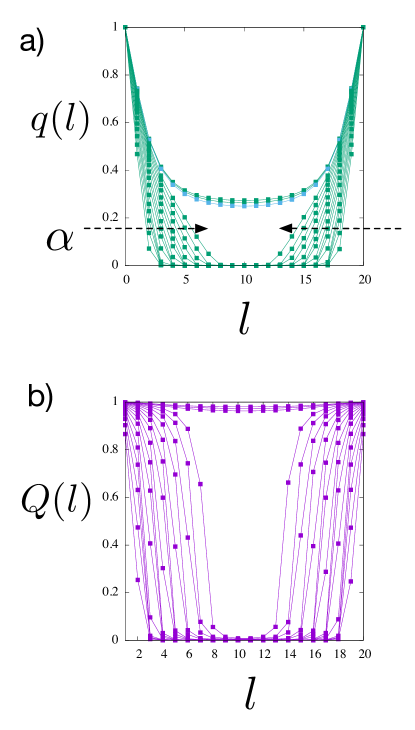
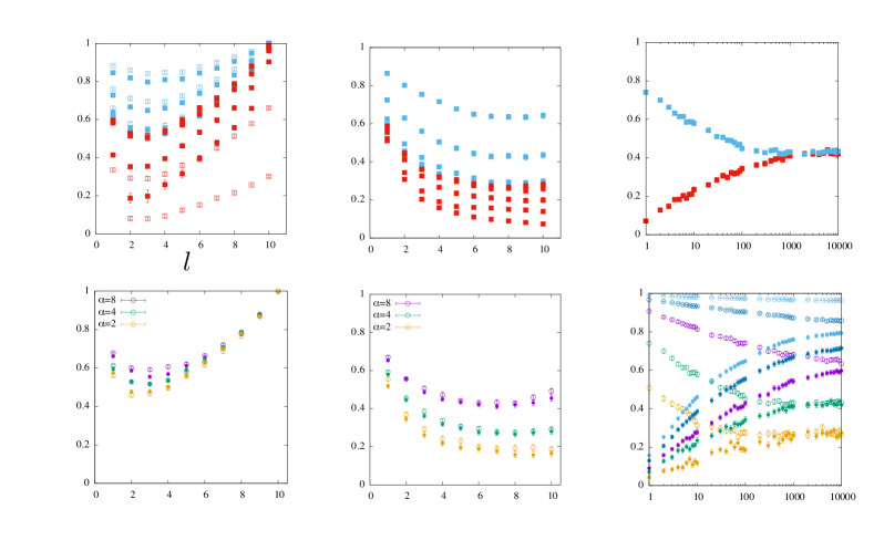
We numerically solved the saddle point equations Eq. (105) to obtain the order parameters repeating the analysis in Yoshino (2020) but in a wider parameter space. In Fig. 7 we show the spatial profile of the order parameters. As already shown in Yoshino (2020), the theory predicts spatially heterogeneous learning. It can be seen that the ’crystalline’ phase with finite order parameter (inference of the teacher’s configuration is successful) grows increasing $\alpha$ starting from the input/output boundaries. This is reminiscent of wetting transitions De Gennes (1985); Krzakala and Zdeborová (2011a, b). Details of the behavior of the order parameters are displayed in Fig. 8.

The central region remains in the liquid phase with zero order parameter (where inference of the teacher’s configuration is impossible) until the two crystalline phases meet in the center at a critical point $\alpha_{c1}(L)$. Naturally $\alpha_{c1}(L)$ increases with $L$. For $\alpha>\alpha_{c1}(L)$ the central liquid phase is absent. As far as $\alpha<\alpha_{c1}(L)$ we find the the crystalline parts attached to the two opposite boundaries grow with $\alpha$ but the profile of the order parameters remain independent of $L$.

Now for $\alpha>\alpha_{c1}(L)$, where the liquid phase is absent, the order parameters depend explicitly on the depth $L$. One may regard this as a ”finite depth $L$ effect”. At some larger $\alpha$ it becomes difficult to follow the saddle point solution numerically. Presumably this implies spinodal instability associated with a first order transition to another solution $q=Q=1$ (which is a saddle point solution) at some $\alpha_{c2}(L)(>\alpha_{c1}(L))$. Such a discontinuous ’perfect recovery’ behavior has been found in the case of single perceptron with binary couplings Györgyi (1990). We skip detailed analysis of the 1st order transition and leave it for future works. Up to the discontinuous change, the evolution of the order parameters with increasing $\alpha$ is continuous.

IV.2.2 Generalization errors

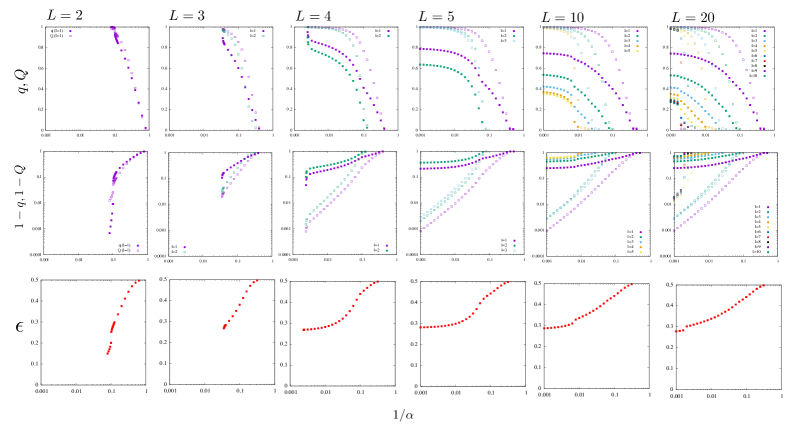
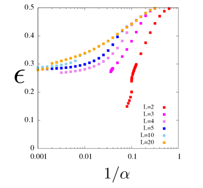
Now we turn to the generalization error $\epsilon$ which is of our main interest in the present paper. It is obtained as shown in the bottom panels of Fig. 8 and Fig. 9. The relation $\epsilon$ vs $\alpha$ is called often as learning curves. Without learning $\alpha=0$, $\epsilon=1/2$ because the student just makes random guesses. The learning curves ${\color[rgb]{0,0,0}\epsilon=\epsilon_{L}(\alpha)}$ consist of two parts as follows.

  • Let us recall that for sufficiently small $\alpha$, the two crystalline phases at the boundaries remain disconnected from each other separated by the liquid phase in the center and that the profile of the order parameters are independent of $L$ since the two crystalline regions do not meet as we discussed in sec. IV.2.1. In this regime the learning curve does not depend on the depth $L$, i. e. $\epsilon=\epsilon_{\infty}(\alpha)$. The reason is that the contribution from the liquid region where $q(l)=Q(l)=0$ to $\epsilon$ Eq. (28) is just zero: it contributes neither positively nor negatively to $\epsilon$. On the other hand, the crystalline region where $q(l),Q(l)>0$ contribute negatively to $\epsilon$ Eq. (28) and it is is independent of $L$ as long as the two crystalline regions do not meet. It is remarkable that $\epsilon_{\infty}(\alpha)<1/2$ and decreases with increasing $\alpha$: the system generalizes even though the central part is in the liquid phase due to over-parametrization.

  • Increasing $\alpha$, the crystalline phases meet at some critical point $\alpha_{c1}(L)$ and the central liquid phase disappear. Note again that $\alpha_{c1}(L)$ is larger for larger $L$. For sufficiently large $\alpha{\color[rgb]{0,0,0}>\alpha_{c1}(L)}$ where the central liquid gap is filled up by the crystalline phase, the learning curve depend on the depth $L$ as the order parameters now depend on $L$. For even larger $\alpha>\alpha_{c2}(L)$, we speculate that $\epsilon$ jumps to 00 due to the 1st order transition mentioned in sec. IV.2.1

The $L$ independent behavior of the learning curve can be seen in Fig. 9 as follows. For instance one can see that $\epsilon_{L}(\alpha)$ of $L=10,20$ are indistinguishable for $1/\alpha>0.01$ and $L=10,20,5$ are indistinguishable for $1/\alpha>0.1$.

Refer to caption
Figure 9: Learning curves of DNN with various depth $L$ obtained by solving the replica symmetric saddle point equations.

IV.3 Finite width $N$ / dimension $D$ effects and finite connectivity $c$ effects

In reality, DNNs have some finite width $N$ and finite connectivity $c$ while in the theory we assumed an idealized situation: the dense limit $N\gg c\gg 1$ and $M\gg 1$ with fixed $\alpha=M/c$. It is very important to consider the effects of finite with $N$ and finite connectivity $c$ (and $M$).

IV.3.1 Finite width $N$ effect

Refer to caption
Figure 10: Schematic picture of the closed and unclosed loop at the boundary

The effects of finite width $N$ can be attributed to the corrections due to geometrically closed loops in the network which becomes non-negligible when the width $N$ is finite as we discussed in sec. III.2. The simplest is the one shown in Fig. 3 which connects adjacent three layers. More extended ones exist as shown in Fig. 20 which connect many layers. As we showed in sec. III.2, the probability to have such a geometrically closed single loop is proportional to $c/N$ no matter how extended it is. The probability vanishes in $N\rightarrow\infty$ but exists as long as $N$ is finite.

Most importantly the loops connect different layers and different nodes within the same layer inducing correlations inside the network. Indeed as discussed in detail sec. B.4 in the appendix, the loops yield finite width $N$ corrections to the interaction part of the free-energy. We also note that the symmetry concerning the exchange of input/output sides present in the saddle point solutions (See Fig. 7) becomes lost in the presence of such loop correction terms.

IV.3.2 Finite hidden dimension $D$ effect

It is interesting to discuss here the hidden manifold model Goldt et al. (2020) introduced in sec. III.7. Let us recall that our original model contains no correlations within the boundaries. We can consider the effect of the correlations put in the input/output boundaries by the hidden manifold model in a perturbative manner around the replica symmetric saddle point solution as the following.

Within the simplest model Eq. (17) for the folding matrix $F$, the same values are repeated in the input (output) data on different nodes $i(=1,2,\ldots,N)$. This amount to induce additional closed loops. For example the unclosed loop in panel b) of Fig. 10 becomes closed if the input data at $k_{1}$ and $k_{2}$ are forced to take the same value by the simplest hidden manifold model. This means that finite width $N$ effects become enhanced as the effective dimension $D$ becomes smaller. This consideration implies finite width $N$ effect and finite hidden dimension $D$ effect will be similar. Both will lead to increase of correlations inside the network.

Let us note that the teacher and students have different architectures in the hidden manifold model so that the inference by the students is not Bayes optimal. In such a circumstance the replica symmetry is not guaranteed. We leave the analysis beyond the perturbative analysis for future works.

IV.3.3 Finite connectivity $c$ effect

Finally, in $N\rightarrow\infty$ limit, we will be still left with finite connectivity $c$ effects. In our theoretical analysis we assumed $c\rightarrow\infty$ which allowed us to perform the saddle point computations. One can naturally consider $1/c$ corrections taking into account contributions from fluctuations around the saddle point as sketched in sec. B.7 in the appendix.

Naturally the fluctuating field around the saddle point induce correlations inside network. Let us also note that the cubic term in the expansion breaks the symmetry concerning the exchange of input/output sides (see sec. B.7.2 in the appendix).

IV.3.4 Discussions

The corrections due to the loops ( sec. IV.3.1) and those due to the fluctuations around the saddle points (sec. IV.3.2) can be easily separated considering the dense limit $N\gg c\gg 1$, which is difficult for the case of global coupling $c=N$. Nonetheless we found that the two corrections bring qualitatively similar effects: 1) correlations inside the network and 2) asymmetry with respect to the exchange of input/output sides.

We consider that the two effects, which disappear in the dense limit, are important in practice in the following respects.

  • Remnant symmetry breaking field

    One would wonder: how a student machine can recognize the existence of the two crystalline regions (teacher’s configuration) if the two are separated by the liquid region as in Fig. 7?”. For an algorithm to work in this situation, some remnant symmetry breaking field should help the student. We consider the corrections due to the loops and the fluctuations around the saddle point play this role.

  • Input-output asymmetry

    One would also wonder: how a DNN with the feed-forward propagation of information can have such spatial profile which is completely symmetric concerning the exchange of input/output sides as in Fig. 7 ? We consider the corrections due to the loops and the fluctuations around the saddle point are responsible for the breaking of this symmetry.

V Simulation

Now let us turn to discuss Monte Carlo simulations on the same model we analyzed theoretically. We first explain the simulation method in sec. V.1, introduce the observables in sec. V.2 and then present the results in sec. V.3.

V.1 Method

V.1.1 Learning scenarios

We simulate the teacher-student scenario (see sec. III.4) in the Bayes-optimal setting and the setting with the hidden manifold model (see sec. III.7).

  • Bayes-optimal scenario

    • Network: teacher and student machines have the same rectangular network of width $N$ and depth $L$ (see Fig. 1). The rectangular network is created as a random graph as the following. Every $\blacksquare\in l$ is given $c$ arms. Each of the arms is connected to a $\blacksquare\in l-1$ chosen randomly out of $N$ possible ones.

    • Synaptic weights of teacher machine: the teacher’s synaptic weights $\{(J_{\blacksquare}^{k})_{\rm teacher}\}$ for $\blacksquare\in 1,2,\ldots,L$ and $k=1,2,\ldots,c$ are prepared as iid random numbers drawn from the Gaussian distribution with zero mean and unit variance.

    • Data: $M$ set of training data is prepared as follows. First the input data for the teacher are prepared as iid random numbers $(S_{\rm teacher})^{\mu}_{0,i}=\pm 1$ for $i=1,2,\ldots,N$ and $\mu=1,2,\ldots,M$. Then the output $(S_{\rm teacher})^{\mu}_{L,i}$ for $i=1,2,\ldots,N$ and $\mu=1,2,\ldots,M$ are obtained by the feed-forward propagation of the signal using Eq. (1). These outputs are used as the target outputs $(S_{*})^{\mu}_{L,i}$ to train the student machines (see below), i. e. $(S_{*})^{\mu}_{L,i}=(S_{\rm teacher})^{\mu}_{L,i}$. Another $M^{\prime}$ set of data for the test (validation) are created in the same way.

  • Hidden manifold scenario Goldt et al. (2020)

    • Network: the networks of the teacher and student machines are the rectangular, random regular network as in the Bayes optimal scenario but the teacher machine is narrower than the student machine, i. e. $D<N$ (see Fig. 6).

    • Synaptic weights of teacher machine: the teacher’s synaptic weights are prepared in the same manner as in the case of the Bayes optimal scenario.

    • Data: $M$ sets of data for training and another $M^{\prime}$ sets of data for the test (validation) are created in the same way as the following. Pairs of input/output data of the teacher’s machine is created just as in the case of Bayes optimal scenario but with $D$ replacing $N$. Then the $N$ dimensional inputs $(S_{\rm student})_{0,i}$ for $i=1,2,\ldots,N$ to be given to the student machines are created using the simple folding matrix $F$ given by Eq. (17). Similarly the $N$ dimensional target output $(S_{*})_{L,i}$ for $i=1,2,\ldots,N$ for the student machines are created using the same folding matrix $F$.

V.1.2 Learning algorithm: greedy Monte Carlo method

For a set of temporal synaptic weights of a student machine $\{(J_{\blacksquare}^{k})_{\rm student}\}$ for $\blacksquare\in 1,2,\ldots,L$ and $k=1,2,\ldots,c$, we obtain the output data $(S_{\rm student})_{L,i}$ ($i=1,2,\ldots,N$) for a given input data $(S_{\rm student})_{0,i}$($i=1,2,\ldots,N$) using the feed-forward propagation based on Eq. (1).

To train the student machines we use a simple zero-temperature or greedy Monte Carlo algorithm. We introduce the loss function defined as,

$$E=\sum_{i=1}^{N}\sum_{\mu=1}^{M}|(S_{\rm student})^{\mu}_{L,i}-(S_{*})^{\mu}_{L,i}|$$ (29)

where $(S_{*})^{\mu}_{L,i}$ is the target output data defined above. Note that the loss function takes discrete values. In particular, we are interested with the ensemble of student machines in the $E=0$ space whose phase space volume is nothing but the Gardner’s volume.

Starting from a set of initial synaptic weights, the student machines are updated as the following.

  1. 1.

    Select a perceptron $\blacksquare$ randomly out of the $N_{\blacksquare}$ possible ones and select a link $k$ randomly out of the $c$ possible ones $k=1,2,\ldots,c$. Then propose a new synaptic weight,

    $$(J_{\blacksquare}^{k})^{\rm new}_{\rm student}=\frac{(J_{\blacksquare}^{k})_{\rm student}+\delta x}{\sqrt{1+\delta^{2}}}$$ (30)

    where $\delta$ is a parameter and $x$ is an iid random number drawn from the Gaussian distribution with zero mean and unit variance. Note that $(J_{\blacksquare}^{k})^{\rm new}_{\rm student}$ is normalized such that its variance remains to be $1$.

  2. 2.

    Accept the proposed one if the resultant loss function does not increase. Otherwise reject it and go back to 1. Importantly we accept updates by which the loss function remains unchanged. This is crucial to allow exploration of the $E=0$ (SAT) space.

Within one Monte Carlo step (MCS) we repeat the above procedure for $N_{\blacksquare}c$ times.

We simulate learning by two student machines ’1’ and ’2’ which are subjected to the same training data but evolve independently from each other using statistically independent random numbers for the step 1. and 2. explained above.

V.1.3 Learning and unlearning

For the training, we consider the following two protocols

  • Learning: the initial synaptic weights of the student machines $\{(J_{\blacksquare}^{k})_{\rm student}\}$ are prepared just as iid Gaussian random numbers totally uncorrelated with the teacher’s weights $\{(J_{\blacksquare}^{k})_{\rm teacher}\}$.

    To facilitate the training, we perform a sort of ’annealing’. At a given time $t$ (MCS), perform the greedy Monte Carlo update using a subset of the training data of size $M_{\rm batch}(t)(<M)$. Starting from $M_{\rm batch}(0)=1$, increase $M_{\rm batch}(t)$ logarithmically in time $t$ progressively adding more data to the training data-set such that $M_{\rm batch}(t_{\rm max})=M$ in the end of the simulation at $t_{\rm max}$ (MCS).

  • Unlearning (or planting): the initial synaptic weights of the student machines $\{(J_{\blacksquare}^{k})_{\rm student}\}$ are set to be exactly the same as the teacher’s weights $\{(J_{\blacksquare}^{k}\}_{\rm teacher}\}$. The student machine explores the $E=0$ (SAT) space.

If the greedy Monte Carlo method equilibrated the system, the two protocols should yield the same results for macroscopic observables, which we explain below, after averaging over time and/or initial configurations in the stationary state.

V.2 Observables

V.2.1 Simple overlaps

We are interested in the similarity between different machines in the hidden layers $l=1,2,\ldots,L-1$. To quantify this we first introduce, between the two student machines ’1’, ’2’ and the teacher machine ’0’, the following ’simple’ overlaps,

$\displaystyle q(l)=\frac{1}{NM}\sum_{i=1}^{N}\sum_{\mu=1}^{M}(S_{1})^{\mu}_{l,i}(S_{2})^{\mu}_{l,j}$ (31)
$\displaystyle r(l)=\frac{1}{2NM}\sum_{i=1}^{N}\sum_{\mu=1}^{M}(S_{0})^{\mu}_{l,j}((S_{1})^{\mu}_{l,i}+(S_{2})^{\mu}_{l,i}).$ (32)

Here $\mu=1,2,\ldots,M$ for the training data and $\mu=1,2,\ldots,M^{\prime}$ for the test data (and replace the factor $1/M$ by $1/M^{\prime}$ in the latter case).

These are the same as the order parameters for the spins used in the replica theory ( see Eq. (18)). However, as mentioned in sec IV.1.1 the expectation value of the simplest overlaps defined above vanish in thermal equilibrium because of the local gauge symmetry (and the permutation symmetry in the case $c=N$) as discussed in sec III.6.

V.2.2 Squared Overlaps

To overcome the above problem we define the following order parameters which we call as squared overlaps which are invariant under the symmetry operations. Let us first introduce,

$\displaystyle q_{ab,ij}(l)$ $\displaystyle=$ $\displaystyle\frac{1}{M}\sum_{\mu=1}^{M}(S_{a})^{\mu}_{l,i}(S_{b})^{\mu}_{l,j}$ (33)

Here $a$ and $b$ are indices for machines: 00 for the teacher machine, $1$ and $2$ for the student machines. Then we introduce the squared overlaps as,

$$q_{2,ab}(l)=\frac{1}{N}\sum_{i,j=1}^{N}(q_{ab,ij}(l))^{2}-\frac{N}{M}$$ (35)

We note that this is analogous to the order parameter used in numerical simulations of vectorial spinglass models which have the rotational symmetry in spin space Hukushima and Kawamura (2000).

Finally we introduce the normalized version of the squared overlap,

$\displaystyle q_{2}(l)$ $\displaystyle=$ $\displaystyle\frac{q_{2,12}(l)}{\sqrt{q_{2,11}(l)}\sqrt{q_{2,22}(l)}}$
$\displaystyle r_{2}(l)$ $\displaystyle=$ $\displaystyle\frac{q_{2,01}(l)+q_{2,02}(l)}{\sqrt{q_{2,00}(l)}(\sqrt{q_{2,11}(l)}+\sqrt{q_{2,22}(l)}}.$ (36)

Interestingly these are very similar to the measure proposed in Kornblith et al. (2019) call as ’centered kernel alignment’.

V.2.3 Nishimori condition

Since our teacher-student scenario is a Bayes optimal inference, we have,

$$q(l)=r(l)\qquad q_{2}(l)=r_{2}(l)\qquad l=1,2,\ldots,L$$ (37)

This is a Nishimori condition which must hold in Bayes optimal inferences Nishimori (2001); Iba (1999); Zdeborová and Krzakala (2016). These relations are useful to check the equilibration of the system.

V.2.4 Physical meaning of the squared overlaps

Let us discuss more closely the significance of the squared overlap defined in Eq. (35) and its normalized version Eq. (36). In the following we denote the average over different realization of the inputs as $\overline{\cdots}^{\rm input}$. From Eq. (LABEL:eq-def-overlap-qij-rij) we can write,

$\displaystyle\overline{(q_{ab,ij}(l))^{2}}^{\rm input}=\frac{1}{M}+\frac{1}{M}\sum_{\mu=1}^{M}\frac{1}{M}\sum_{\nu(\neq\mu)}\overline{r_{a,i}^{\mu\rightarrow\nu}r_{b,j}^{\mu\rightarrow\nu}}^{\rm input}$
$\displaystyle\simeq\frac{1}{M}+\overline{r_{a,i}^{\mu\rightarrow\nu(\neq\mu)}r_{b,j}^{\mu\rightarrow\nu(\neq\mu)}}^{\rm input}$ (38)

with

$\displaystyle r_{a,i}^{\mu\rightarrow\nu}=(S_{a})^{\mu}_{li}(S_{a})^{\nu}_{li}$ (39)

Here $r_{a,i}^{\mu\rightarrow\nu}$ can be regarded as change of the sign of the spin (neuron) at the node $(l,i)$ of the student-a when the input pattern is changes from $\mu$ to $\nu$. Using the above expression we find Eq. (35) with the subtraction term $-N/M$ becomes,

$$q_{2,ab}(l)\simeq\frac{1}{N}\sum_{j=1}^{N}\overline{r_{a,i}^{\mu\rightarrow\nu(\neq\mu)}r_{b,j}^{\mu\rightarrow\nu(\neq\mu)}}^{\rm input}$$ (40)

This can be viewed as a kind of correlation volume within layer $l$ in the following sense.

  • Totally uncorrelated random machines

    Suppose that the student-a and student-b are totally uncorrelated (far beyond the trivial difference by the gauge transformation and the permutation) randomly generated machines. Then we naturally expect $\overline{r_{a,i}^{\mu\rightarrow\nu(\neq\mu)}r_{b,j}^{\mu\rightarrow\nu(\neq\mu)}}^{\rm input}=0$. This means that the minimum value of the squared overlap $q_{2,ab}(l)$ is 00.

  • Same random machine modulo gauge transformation and permutation

    On the other hand, if the two machines are the same machine modulo the gauge transformation and permutation we can write

    $$\overline{r_{a,i}^{\mu\rightarrow\nu(\neq\mu)}r_{b,j}^{\mu\rightarrow\nu(\neq\mu)}}^{\rm input}=\delta_{ij}+(1-\delta_{ij})\overline{r_{a,i}^{\mu\rightarrow\nu(\neq\mu)}r_{b,j}^{\mu\rightarrow\nu(\neq\mu)}}^{\rm input}$$ (41)

    Thus in this case the squared overlap $q_{2,ab}(l)$ is at least $1$ and can be larger.

    In the case of the perceptrons with random synaptic weights and the highly non-linear activation function (see Eq. (1)), we expect $\overline{r_{a,i}^{\mu\rightarrow\nu(\neq\mu)}r_{b,j}^{\mu\rightarrow\nu(\neq\mu)}}^{\rm input}$ becomes significant also between different nodes $i\neq j$. This is because of the chaos effect which we discussed in sec. III.3: it is known that in such a non-linear random feed-forward network a slight change of the input induces chaotic changes in the state of spins (neuron) as the signal propagates deeper into the network Poole et al. (2016). This is an avalanche-like process so that the correlation $\overline{r_{a,i}^{\mu\rightarrow\nu(\neq\mu)}r_{b,j}^{\mu\rightarrow\nu(\neq\mu)}}^{\rm input}$ for $i\neq j$ becomes more significant increasing $l$. In this case the squared overlap $q_{2,ab}(l)$ can be viewed as a measure of avalanche size within layer $l$.

  • General case

    Based on the above consideration, we naturally expect that in general $q_{2,ab}(l)$ quantifies the avalanche size and similarity of the avalanche patterns taking place in machines a and b through changes of inputs $\mu\rightarrow\nu(\neq\mu)$. Then it becomes clear that normalized version Eq. (36) quantifies the quantifies the similarity of the avalanche patterns in machines a and b.

V.2.5 Generalization error

To measure the generalization ability of the student machines (see sec. III.4) we measure,

$$r_{\rm out}=\frac{1}{NM}\sum_{i=1}^{N}\sum_{\mu=1}^{M^{\prime}}(S_{\rm student})^{\mu}_{l,i}(S_{\rm teacher})^{\mu}_{l,i}$$ (42)

Here we use the $M^{\prime}$ sets of the outputs of the teacher and student machines for the test data (not used for training). The generalization error (see Eq. (12)) can be evaluated as,

$$\epsilon=\frac{1}{2}(1-r_{\rm out}).$$ (43)

In the above expression, we used simple overlap defined on the output layer $l=L$. Note that there are no gauge transformations or permutations on the output layer.

Refer to caption
Figure 11: Relaxation of the loss function in learning (annealing with $t_{\rm max}=10^{4}$ (MCS)) observed by the MC simulation. In all cases $N=10$. (a) various $\alpha=M/c$ with $L=10$ and $c=5$. (b) various $L$ with $\alpha=M/c=4$ and $c=5$. (c) various $N$ with $L=10$, $\alpha=4$ and $c=5$. (d) the same as (c) but with $c=10$. The unit of time $t$ is $1$ (MCS).
Refer to caption
Figure 12: Time evolution of simple student-student overlap $q(l)$ (filled symbols) and teacher-student overlap $r(l)$ (open symbols) observed in MC simulations of the unlearning protocol. Here $N=10$, $\alpha=4$, $c=5$. Panel a) shows data at $t=1,2,4,8,10,20,40,80$. Panels b) and c) show the simple student-student overlap $q(l)$ and simple teacher-student $r(l)$ overlap respectively.

V.3 Results

Now let us discuss the results of the simulations. First, we discuss the equilibration process through the learning and unlearning protocols (see sec. V.1.3). Next, we discuss the equilibrium properties of macroscopic observables.

In the simulations we used $\delta=0.1$ to generate new weights by Eq. (30). For the test we used $M^{\prime}=M$ data uncorrelated with the training data. In the following observables are averaged are took over statistically independent $240$ samples (different realizations of the teacher machine, initial configurations of student machines for learning, realizations of random numbers used in Monte Carlo updates).

V.3.1 Learning

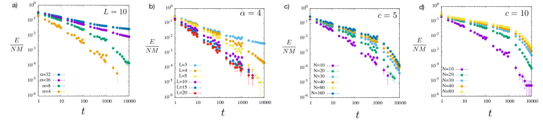
In Fig. 11 we present the relaxation of the loss function Eq. (29) in the learning protocol (see sec. V.1.3). It can be seen in panel a) that relaxation of the loss function slows down by increasing the number of the training data $M=c\alpha$. On the other hand, it can be observed in panel b) that relaxation becomes faster increasing the depth $L$ of the network.

As shown in panel c), the relaxation depends also on the width $N$ but converges in large enough $N$ with fixed $c$ and $\alpha$ suggests that relaxation time is finite in systems with finite connectivity $c$ even in $N\rightarrow\infty$ limit. For larger $c$, the relaxation curves converge to a slower curve as shown in panel d) suggesting that the relaxation time becomes larger for larger connectivity $c$.

V.3.2 Unlearning

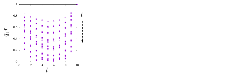
In Fig. 12 we show the simple overlaps defined in Eq. (32) observed in the unlearning protocol which explores the $E=0$ landscape (SAT phase) (see sec. V.1.3). Note that $q(l)=r(l)=1$ at the beginning. The student machines become de-correlated from the teacher machine and also de-correlated from each other as time $t$ elapses. It is interesting to note that relaxation is in-homogeneous in space: relaxation is faster in the central part of the network and slower closer to the input/output boundaries.

It is important to note that the complete vanishing of the simple overlaps does not necessarily mean that the solution space is completely in a liquid state as the overlaps are not gauge invariant. Because of the gauge symmetry (see sec III.6.1), even machines that are completely the same as the teacher-machine modulo the gauge transformation can have vanishing simple overlap with the teacher-machine. Indeed we will find below that normalized squared overlaps Eq. (36) (which are gauge invariant) instead indicate correlations between different machines.

The in-homogeneity of the relaxation observed here suggests that the system is more constrained closer to the boundary while the center is freer. We have also observed that the deeper system relax faster as shown in Fig. 11 b). These may be interpreted as an echo of the ’crystal-liquid-crystal’ sandwich structure predicted by the theory (Fig. 7).

Refer to caption
Figure 13: Spatial profile of the normalized squared teacher-student overlaps $r_{2}(l)$ and student-student overlaps $q_{2}(l)$ (see Eq. (36)) for training a),b) and test c),d) and time evolution of the simple teacher-student overlap $r(L)$ in the output layer ($l=L$) for test e), f). All data are obtained by the MC simulations. In panels a), c), and e), data of $q_{2}(l)$ (open symbols) and $r_{2}(l)$ (filled symbols) of learning/unlearning are represented by red/blue points ($\alpha=4$) . Panels a) and c) show the normalized squared overlaps at various times $t=1,10,100,1000,10000$ (increasing along the arrows) at each layer. Panel e) shows the time evolution of the simple teacher-student overlap $r(L)$ at the output layer ($l=L$) for the test data. Panel b) and d) show the normalized squared teacher-student overlap for unlearning (open symbols)/learning (filled symbols) at $\alpha=2,4,8$ at $t=10^{4}$ (MCS). Panel f) show the time evolution of the simple teacher-student overlap $r(L)$ at the output layer ($l=L$) for the test data, obtained by unlearning (open symbols) /learning (filled symbols) protocols with $\alpha=2,4,8,16,32$. Here $N=10$, $L=10$, and $c=5$ for all data.

V.3.3 Equilibration

In equilibrium learning and unlearning protocols should give the same results for macroscopic observables after sufficiently long times. This is indeed verified as shown in the top panels a) c) e) of Fig. 13. In panels a) and c) we show the normalized squared overlaps defined in Eq. (36) which are invariant under the gauge transformations. The normalized squared overlaps of unlearning and learning protocols agree suggesting the establishment of equilibrium. Furthermore, it can be seen that the Nishimori condition $q_{2}(l)=r_{2}(l)$ (see Eq. (37)) expected for the Bayes optimal inferences become satisfied after sufficiently long times. This is another evidence of thermal equilibration. Equilibration can also be seen in panel e) where we show the simple overlap between the teacher and student machines in the output layer $l=L$ for the test data.

As can be seen in Fig. 13, the spatial profile of the normalized squared overlaps $q_{2}(l)$ and $r_{2}(l)$ are strongly in-homogeneous in space. As discussed in sec. V.2.4, we consider the normalized squared overlaps quantifies the similarity of the avalanche patterns taking place in different machines through changes of inputs $\mu\rightarrow\nu(\neq\mu)$. At the beginning of unlearning, which starts from the teacher’s configuration, the normalized squared overlaps take high values. On the other hand, they are small at the beginning of learning which is not surprising because teacher and student machines are totally uncorrelated at the beginning. In equilibrium, they converge to a non-trivial, spatially non-monotonic function. This implies that the equilibrium phase is not just a liquid as we might have thought based on the observation of the vanishing simple overlap (Fig. 12). On the contrarily, the gauge invariant quantity show that the student machines are strongly correlated with each other and with the teacher machine in equilibrium. The spatial non-monotonicity means that they become less correlated with each other in the center (beyond the trivial difference by the gauge transformations) while they are similar to each other (modulo the gauge transformation) closer to the input and output boundaries. This observation can be regarded as another echo of the spatial in-homogeneity predicted by the theory (Fig. 7). From the theoretical point of view, the strong asymmetry concerning the exchange of input/output sides, which is absent in the saddle point solution, may be attributed to the finiteness of the width $N$ and the connectivity $c$ as we discussed in sec. IV.3.4.

As shown in the bottom panels b) d) f) in Fig. 13, the overlaps increase as $\alpha$ increases as expected. In panel f) it can be seen that dynamics of both learning and unlearning slow down as $\alpha$ increases.

V.3.4 Typical student machines

Refer to caption
Figure 14: Finite $N$ effect and finite $c$ effect: the asymmetry becomes smaller as $N$ increases for unlearning (open symbols) /learning (filled symbols). $N=10,20,30,40,80$ with $\alpha=1.0$ and (left) $c=5$, (right) $c=10$ . All data are obtained by MC simulations of $t=10^{4}$ (MCS).
Refer to caption
Figure 15: Spatial profile of the normalized squared overlaps and the generalization error in systems with various width $N$ (top panels) and hidden dimension $D(\leq N)$ (bottom panels) obtained by MC simulations. In the top panels, data obtained by both learning (filled symbols) and unlearning (open symbols) are shown. Panels a) and b) show the normalized squared overlaps for training, c) and d) show those for the test. Panels e) and f) show the generalization error $\epsilon$ (see Eq. (43)). In panel e) we also show the generalization error $\epsilon$ obtained by the theory in the dense limit: $N\rightarrow\infty$ followed by $N\rightarrow\infty$ (see Eq. (12) and Fig. 9). In panels a), b), c), and d) data with $L=5,10,20$ are shown. In panels a), c), and e) data with $N=8,10,20$ are shown. In panels b), d) and f) data with $D=4,6,8,10$ are shown. In all cases $\alpha=4$, $c=5$ and $t=10^{4}$.

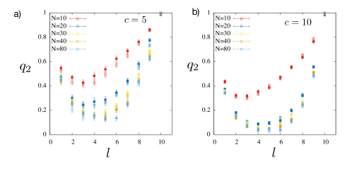
Now let us examine further the equilibrium properties, i. e. properties of typical student machines sampled in the solution space. We show in Fig.  14 some data of the normalized squared overlaps $q_{2}(l)$. It can be seen again that the data obtained by both learning (filled symbols) and unlearning (open symbols) agree confirming that the system is equilibrated. Quite remarkably the equilibrium normalized squared overlap $q_{2}(l)$ evolves non-monotonically in space for large enough $N$ and $c$. It first decreases with $l$ but finally increases with $l$. This means avalanches taking place in different machines become de-correlated in the middle of the network but strongly correlated closer to the input and output boundaries. It appears that the situation has become closer to the ’crystal-liquid-crystal’ sandwich structure predicted by the theory (Fig. 7) increasing $N$ and $c$.

In sec. IV.3.4 we discussed that the corrections due to the loops and fluctuations around the saddle point can be separated considering the dense limit $N\gg c\gg 1$ but bring similar effects 1) remnant symmetry breaking field 2) input-output asymmetry. Indeed it can be seen in Fig.  14 that for fixed connectivity $c$, the normalized squared overlaps decrease around the center of the network and the asymmetry with respect to the exchange of input/output becomes weaker as $N$ increases. Furthermore, the data suggests convergence in $N\rightarrow\infty$ limit with fixed $c$. Comparing panels a) and b) it can be seen that the remnant asymmetry becomes weaker as the connectivity $c$ increases. Remarkably de-correlation in the center also becomes clearer increasing $N$ and $c$, suggesting the emergence of liquid like region in the center due to over-parametrization as suggested theoretically in the dense limit $N\gg c\gg 1$.

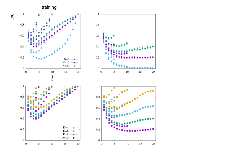
In Fig. 15 we show the normalized squared overlaps $q_{2}(l)$, $r_{2}(l)$ and the generalization error $\epsilon$ in systems with $\alpha=4$, $c=5$ observed after $t=10^{4}$ (MCS) in systems with different depth $L=5,10,20$. As shown in the top panels a) c) and e) data obtained by both learning (filled symbols) and unlearning (open symbols) agree proving again that the system is equilibrated. As shown in panels a) and c) we find again that the normalized squared overlaps are strongly in-homogeneous in space. The machines de-correlate more concerning each other in the central region in deeper systems but correlations recover approaching the output layer. We also find again that normalized squared overlaps increase significantly and that the asymmetry concerning the exchange of the input and output sides becomes stronger decreasing the width $N$.

Now let us turn to the effect of finite dimension $D$ introduced by the hidden manifold model (see sec. V.1.1). The results of simulations on the hidden manifold model are displayed in panels b) and d) of Fig. 15. Here we used the simplest folding matrix $F$ of the form Eq. (17) but we obtained qualitatively the same results (not shown) also in the case of random matrices. Comparing the panels b) to a) and d) to c) we immediately notice that the effect of hidden dimension $D$ is quite similar to the effect of finite width $N$: decreasing $D$ with fixed $N$ is much like decreasing $N(=D)$. We conjecture that this is due to the enhancement of the loop corrections induced by the closing of the loops by the correlated inputs as discussed in sec. IV.3.2.

Finally, let us discuss the generalization error $\epsilon$ shown in panels e) and f) of Fig. 15. In panel e) we also show the generalization error $\epsilon$ obtained by the theory in the dense limit $c\rightarrow\infty$ (see Eq. (12) and Fig. 9). Remarkably the effect of finite width $N$ and hidden dimension $D$ is very similar again. The generalization error improves significantly either by decreasing $N(=D)$ or $D$ with fixed $N$. Presumably this is due to the increase of correlations inside the network induced by the loop corrections. Moreover, the generalization error becomes independent of the depth $L$ at sufficiently deep systems much like the theoretical prediction. The result implies the generalization ability first decreases making the system deeper but does not vanish even in $L\rightarrow\infty$ limit. This is consistence with the $L$ independent learning curve $\epsilon=\epsilon_{\infty}(\alpha)$ predicted theoretically (see sec. IV.2.2).

VI Conclusions

In the present paper we obtained an exactly solvable statistical mechanics model of machine learning by a deep neural network (DNN) in the dense limit $N\gg c\gg 1$. Exact solutions are obtained using the replica method developed in Yoshino (2020). We used the replica theory to analyze the generalization-ability of the DNN in the Bayes-optimal teacher-student setting. The learning curve $\epsilon=\epsilon_{L}(\alpha)$ becomes independent of of the depth $L$ as long as the two crystalline phases attached to input/output boundaries are separated by the liquid phase in the center. Thus the system is predicted to generalize even in the limit $L\rightarrow\infty$ where the system becomes extremely over-parametrized. We discussed the loop corrections to the dense limit and argued that finite width $N$ and finite hidden dimension $D$ effects appear similarly. Both should lead to increase of correlations inside the network.

In simulations, the simple greedy Monte Carlo method turned turned out to work efficiently to enable sampling of typical machines in equilibrium suggesting the simplicity of the loss landscape. The main obstacle in simulations is the gauge invariance of the system by which order parameters in the original simple form vanish. To overcome the difficulty we measured normalized squared overlap which quantifies the correlation of avalanches concerning changes in input data between different machines. It is a gauge (and permutation) invariant quantity that reflects the similarity between machines modulo the gauge (and permutation) symmetries. The result is qualitatively consistent with the theoretical prediction that over-parametrization in the DNN lead to spatially in-homogeneous learning: students become close to the teacher around the input/output boundaries while remain only weakly correlated in the center. We note that liquid like central region was also noticed in Zou and Huang (2021). Furthermore, somewhat counter-intuitively but in agreement with the theoretical prediction, the generalization error first increases increasing the depth $L$ but then becomes independent of the depth $L$ suggesting that the generalization ability survives in $L\rightarrow\infty$ limit. Simulations confirm that finite width $N$ and finite hidden dimension $D$ effects are quite similar and lead similarly to significant improvements in the generalization ability. Presumably this reflects increase of correlations inside the network due to the loop corrections. As we noted in sec. IV.3.4 we consider that the corrections due to the loops and fluctuations around the saddle point play the role of symmetry breaking field which allows the student to recognize again the teacher in spite of the liquid like center.

After all what is the advantage of making the system deeper? One important advantage is that the learning dynamics become faster increasing the depth as we found numerically. This should be due to the presence of the central region where the system is less constrained. We believe that this point will become more important as we move away from the idealized, Bayes optimal teacher-student setting we considered in the present work. From the theoretical point of view, there is no guarantee that replica symmetry continue to hold as we move away from the Bayes optimal situation toward the situations in the real world. For example, one can consider a noisy teacher-student scenario by adding noise to the training data provided by the teacher. Then the situation becomes closer to the random scenario considered in Yoshino (2020) where complex replica symmetry breaking (RSB) was found in the DNN. In the latter case, RSB evolves in space such that the hierarchy of RSB becomes simplified layer-by-layer approaching the center so that the central region can remain in replica symmetric liquid phase if the network is made deep enough. This implies deeper system will relax faster even in the presence of the RSB around the boundaries.

There are numerous directions to generalize and extend the present work. Let us mention a few of them below. It is straightforward to study the model exactly with the parameter $\alpha$ depending on space $\alpha=\alpha(l)$. This amount to make the width $N$ of the network to vary in space $N=N(l)$. It will be interesting to study how one can control the spatial heterogeneity of learning by changing $\alpha(l)$. The dense limit $N\gg c\gg 1$ will be useful not only for the replica theory but other theoretical approaches. For instance, it should be possible to develop cavity approaches in the dense limit. It will also be very interesting to generalize our theory considering more general activation functions as we noted in sec. III.3.

Acknowledgments

We thank Giulio Biroli, Angelo Giorgio Cavaliere, Yoshiyuki Kabashima and Ryo Karakida for useful discussions. Numerical simulations presented in this work has been done using the supercomputer systems SQUID at the Cybermedia Center, Osaka University. This work was supported by KAKENHI (No. 21K18146) (No. 22H05117) from MEXT, Japan.

Appendix A Transfer matrix representation of feed-forward networks

Here we show that transfer-matrix representations of a family of spin-glass models put in the layered geometry (like in Fig. 1) become feed-forward DNNs in the zero temperature limit.

In the following we denote the configuration of the set of spins in the $l$-th layer as ${\bf S}_{l}^{\mu}=\{S_{\blacksquare\in l}^{\mu}\}$ where $\mu$ is the label to specify a data set. Let us write the conditional probability to realize a spin configuration ${\bf S}^{\mu}_{L}$ on the output boundary given a spin configuration ${\bf S}^{\mu}_{0}$ on the input boundary as,

$$P({\bf S}^{\mu}_{0}\rightarrow{\bf S}^{\mu}_{L})=\left(\prod_{l=1}^{L-1}{\rm Tr}_{{\bf S}^{\mu}_{l}}\right)\prod_{l=1}^{L}P({\bf S}^{\mu}_{l-1}\rightarrow{\bf S}^{\mu}_{l})$$ (44)

where $P({\bf S}^{\mu}_{l-1}\rightarrow{\bf S}^{\mu}_{l})$ is the conditional probability to realize a spin configuration ${\bf S}^{\mu}_{l}$ on the $l$-th layer given a spin configuration ${\bf S}^{\mu}_{l-1}$ on the $l-1$-th layer,

$\displaystyle P({\bf S}^{\mu}_{l-1}\rightarrow{\bf S}^{\mu}_{l})$ $\displaystyle=$ $\displaystyle\frac{\langle{\bf S}_{l-1}^{\mu}|{\bf T}_{l}|{\bf S}_{l}^{\mu}\rangle}{{\rm Tr}_{{\bf S}^{\mu}_{l}}\langle{\bf S}_{l-1}^{\mu}|{\bf T}_{l}|{\bf S}_{l}^{\mu}\rangle}$ (45)

where ${\bf T}_{l}$ is the transfer matrix from the $l-1$ to $l$ th layer.

A.1 Layered Ising spin-glass model

Let us first consider the layered Ising spin-glass model Eq. (4) with the restricted Boltzmann machine (RBM) like architecture Ackley et al. (1985),

$$H=-\frac{1}{\sqrt{c}}\sum_{\blacksquare}\sum_{k=1}^{c}J_{\blacksquare}^{k}S_{\blacksquare}S_{\blacksquare(k)}$$ (46)

where the spins are Ising variables $S^{\mu}=\pm 1$. The matrix elements of the transfer matrix are given by,

$$\langle{\bf S}^{\mu}_{l-1}|{\bf T}_{l}|{\bf S}^{\mu}_{l}\rangle=e^{\sum_{\blacksquare\in l}\sum_{k=1}^{c}\frac{\beta J_{\blacksquare}^{k}}{\sqrt{c}}S_{\blacksquare}^{\mu}S^{\mu}_{\blacksquare(k)}}$$ (47)

Here $\beta=1/T$ is the inverse of the temperature $T$. The size of the matrix is $2^{N}\times 2^{N}$. Then we find the conditional probability Eq. (45) becomes,

$$P({\bf S}^{\mu}_{l-1}\rightarrow{\bf S}^{\mu}_{l})=\prod_{\blacksquare\in l}P({\bf S}^{\mu}_{l-1}\rightarrow S^{\mu}_{\blacksquare})$$ (48)

where

$$\prod_{\blacksquare\in l}P({\bf S}^{\mu}_{l-1}\rightarrow S^{\mu}_{\blacksquare})=\prod_{\blacksquare\in l}\frac{e^{\beta r_{\blacksquare}^{\mu}}}{{\rm Tr}_{S_{\blacksquare}^{\mu}}e^{\beta r_{\blacksquare}^{\mu}}}$$ (49)

with $r_{\blacksquare}^{\mu}$ being the gap variable Eq. (10),

$$r_{\blacksquare}^{\mu}=S_{\blacksquare}^{\mu}\sum_{k=1}^{c}\frac{J_{\blacksquare}^{k}}{\sqrt{c}}S^{\mu}_{\blacksquare(k)}$$ (50)

It is important to notice the factorization of the conditional probability in Eq. (48). It is the consequence of the RBM type architecture: there are no direct interactions within each layer.

Taking the zero temperature limit $T\rightarrow 0$ ($\beta\rightarrow\infty$) we find,

$$P({\bf S}^{\mu}_{l-1}\rightarrow{\bf S}^{\mu}_{l})\xrightarrow[T\rightarrow 0]{}\prod_{\blacksquare\in l}\theta(r_{\blacksquare}^{\mu})$$ (51)

where $\theta(r)$ being the Heviside step function. Thus in this limit the configuration $S_{\blacksquare}^{\mu}$ in $\blacksquare\in\l$ is determined deterministically given ${\bf S}^{\mu}_{\square}$ in $\square\in l-1$ by the perceptron’s rule Eq. (1),

$$S_{\blacksquare}^{\mu}={\rm sgn}\left(\sum_{k=1}^{c}\frac{J_{\blacksquare}^{k}}{\sqrt{c}}S^{\mu}_{\blacksquare(k)}\right)$$ (52)

Note that the operation of the transfer matrix of size $2^{N}\times 2^{N}$ Eq. (47) is now replaced in the $T\rightarrow 0$ limit by simple non-linear mapping of much lower computational cost of $O(Nc)$ thanks to the 1) RBM like network structure and 2) $T\rightarrow 0$ limit.

Similarly we find,

$$\lim_{T\rightarrow 0}P({\bf S}^{\mu}_{0}\rightarrow{\bf S}^{\mu}_{L})=\left(\prod_{\blacksquare\backslash{\rm output}}{\rm Tr}_{{\bf S}^{\mu}_{\blacksquare}}\right)\prod_{\blacksquare}\theta(r_{\blacksquare}^{\mu})$$ (53)

which means $S_{\blacksquare\in L}$ in the output layer becomes determined by the multi-layer perceptron for a given $S_{\blacksquare\in 0}$ in the output layer. Note that the Gardner’s volume Eq. (8) can be written as,

$$V_{M}\left({\bf S}_{0},{\bf S}_{L}\right)=\lim_{T\rightarrow 0}\left(\prod_{\blacksquare}{\rm Tr}_{{\bf J}_{\blacksquare}}\right)\prod_{\mu}P({\bf S}^{\mu}_{0}\rightarrow{\bf S}^{\mu}_{L})$$ (54)

In this representation it becomes clear that the traces over the spins in the hidden layers used in the Gardner’s volume for DNN Eq. (8) (the internal representation Monasson and Zecchina (1995)) are equivalent to computation of the products of transfer-matrices in Eq. (44).

A.2 Layered spin-glass models with continuous spins

Now let us consider a class of slightly more generalized models on the RBM type network with the Hamiltonian,

$$H=-\frac{1}{\sqrt{c}}\sum_{\blacksquare}\sum_{k=1}^{c}J_{\blacksquare}^{k}S_{\blacksquare}S_{\blacksquare(k)}+\sum_{\blacksquare}U(S_{\blacksquare})$$ (55)

Here we consider spins which take continuous values $-\infty<S<\infty$. The function $U(x)$ in the 2nd term of the Hamiltonian Eq. (55) represents a confining potential to regularize the spins. Then the conditional probability Eq. (45) becomes,

$\displaystyle P({\bf S}^{\mu}_{l-1}\rightarrow{\bf S}^{\mu}_{l})$ $\displaystyle=$ $\displaystyle\prod_{\blacksquare\in l}\frac{e^{\beta(h_{\blacksquare}^{\mu}S_{\blacksquare}^{\mu}-U(S_{\blacksquare}^{\mu}))}}{{\rm Tr}_{S_{\blacksquare}^{\mu}}e^{\beta(h_{\blacksquare}^{\mu}S_{\blacksquare}^{\mu}-U(S_{\blacksquare}^{\mu}))}}$ (56)

where

$$h_{\blacksquare}^{\mu}=\sum_{k=1}^{c}\frac{J_{\blacksquare}^{k}}{\sqrt{c}}S^{\mu}_{\blacksquare(k)}$$ (57)

In $T\rightarrow 0$ limit we find,

$\displaystyle P({\bf S}^{\mu}_{l-1}\rightarrow{\bf S}^{\mu}_{l})$ $\displaystyle\rightarrow$ $\displaystyle\prod_{\blacksquare\in l}\delta\left({\bf S}^{\mu}_{\blacksquare}-f(h^{\mu}_{\blacksquare})\right)$ (58)

where the function $f(h)$ is determined such that

$$f(h)={\rm argmin}_{S}\left({\color[rgb]{0,0,0}-hS+U(S)}\right)$$ (59)

Assuming that the potential $U(s)$ is differentiable we find,

$$f^{-1}(S)={\color[rgb]{0,0,0}\frac{dU(S)}{dS}}$$ (60)

or

$$U(S)=\int_{-\infty}^{S}f^{-1}(S)dS$$ (61)

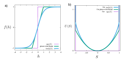
Thus given a layered spin-glass model with a confining local potential $U(S)$ Eq. (55) we find a corresponding feed-forward neural network with the activation function $f(h)$ in $T\rightarrow 0$ limit.

In Fig. 16 we display some examples of activation functions $f(h)$ and the associated confining potentials $U(S)$. In sec A.1 we showed that the transfer-matrix of layered Ising spin-glass model becomes equivalent to the feed-forward network with the activation function $f(h)={\rm sgn}(h)$ in $T\rightarrow 0$ limit. The same activation function can be obtained also from the continuous spin model using confining potential

$$U(S)=\left\{\begin{array}[]{cc}0&(-1<u<1)\\ \infty&(u<-1\qquad\mbox{or}\qquad u>1)\end{array}\right.$$ (62)

Similarly, for a piece wise linear function parametrized by $u>0$,

$$f(h)=\left\{\begin{array}[]{cc}1&(h>u)\\ \frac{h}{u}&(-u<h<u)\\ -1&(h<-u)\end{array}\right.$$ (63)

we find

$$U(S)=\left\{\begin{array}[]{cc}\frac{u}{2}\left(S-\frac{h}{u}\right)^{2}+\frac{h^{2}}{u}&(-1<u<1)\\ \infty&(u<-1\qquad\mbox{or}\qquad u>1)\end{array}\right.$$ (64)

Finally in the case of $f(h)=\tanh(h)$ one can easily find $U(S)=S\tanh^{-1}(S)+(1/2)\ln(1-S^{2})$.

Refer to caption
Figure 16: Some examples of the activation function $f(h)$ and the associated confining potential $U(S)$. Here $u=1$ for the piece-wise linear function.

Appendix B Details of the replica theory

B.1 Replicated Gardner volume, Fourier transformation, and Legendre transformation

By introducing a Fourier representation of the Boltzmann factor,

$$e^{-\beta v(r)}=\int\frac{d\eta}{\sqrt{2\pi}}W_{\eta}e^{-i\eta r}.$$ (65)

the replicated Gardner volume Eq. (21) can be rewritten as,

$\displaystyle V^{n}\left({\bf S}_{0},{\bf S}_{L}\right)=e^{NM{\cal S}_{n}\left({\bf S}_{0},{\bf S}_{l}\right)}$ (66)
$\displaystyle=$ $\displaystyle\prod_{a}\left(\prod_{\blacksquare}{\rm Tr}_{{\bf J}^{a}_{\blacksquare}}\right)\left(\prod_{\blacksquare\backslash{\rm output}}{\rm Tr}_{{\bf S}^{a}_{\blacksquare}}\right)\left\{\prod_{\mu,\blacksquare,a}e^{-\beta v(r_{\blacksquare,a}^{\mu})}\right\}$
$\displaystyle=$ $\displaystyle\prod_{\mu,\blacksquare,a}\left\{\int\frac{d\eta_{\mu,\blacksquare,a}}{\sqrt{2\pi}}W_{\eta_{\mu,\blacksquare,a}}\right\}\tilde{V}^{n}\left({\bf S}_{0},{\bf S}_{L}\right)$

where we introduced the Fourier transform of the replicated Gardner volume

$\displaystyle\tilde{V}^{n}\left({\bf S}_{0},{\bf S}_{L}\right)$ $\displaystyle=$ $\displaystyle\prod_{a}\left(\prod_{\blacksquare}{\rm Tr}_{{\bf J}^{a}_{\blacksquare}}\right)\left(\prod_{\blacksquare\backslash{\rm output}}{\rm Tr}_{{\bf S}^{a}_{\blacksquare}}\right)$ (67)
$\displaystyle\prod_{\mu,\blacksquare,a}e^{i\eta_{\mu,\blacksquare,a}r_{\blacksquare,a}^{\mu}}$

with the gap variable $r^{\mu}_{\blacksquare,a}$ defined as

$$r^{\mu}_{\blacksquare,a}\equiv(S^{\mu}_{\blacksquare})^{a}\sum_{k=1}^{c}\frac{(J_{\blacksquare}^{k})^{a}}{\sqrt{c}}(S^{\mu}_{\blacksquare(k)})^{a}$$ (68)

Introducing identities

$\displaystyle 1$ $\displaystyle=$ $\displaystyle\prod_{a<b}\int_{-\infty}^{\infty}\int_{-i\infty}^{i\infty}\left(\frac{c}{2\pi i}\right)dQ_{ab,\blacksquare}d\epsilon_{ab,\blacksquare}e^{c\sum_{a<b}\epsilon_{ab,\blacksquare}\left(Q_{ab,\blacksquare}-c^{-1}\sum_{k=1}^{c}(J_{\blacksquare}^{k})^{a}(J_{\blacksquare}^{k})^{b}\right)}$
$\displaystyle 1$ $\displaystyle=$ $\displaystyle\prod_{a<b}\int_{-\infty}^{\infty}\int_{-i\infty}^{i\infty}\left(\frac{M}{2\pi i}\right)dq_{ab,\blacksquare}d\varepsilon_{ab,\blacksquare}e^{M\sum_{a<b}\varepsilon_{ab,\blacksquare}\left(q_{ab,\blacksquare}-M^{-1}\sum_{\mu=1}^{M}(S_{\blacksquare}^{\mu})^{a}(S_{\blacksquare}^{\mu})^{b}\right)}$ (69)

we can express the Fourier transformation of the replicated Gardner volume $\tilde{V}^{n}$ as,

$\displaystyle\tilde{V}^{n}\left({\bf S}_{0},{\bf S}_{L}\right)$ $\displaystyle=$ $\displaystyle\prod_{a<b,\blacksquare}\left\{\int_{-\infty}^{\infty}dQ_{ab,\blacksquare}\right\}\prod_{a<b,\blacksquare\backslash{\rm output}}\left\{\int_{-\infty}^{\infty}dq_{ab,\blacksquare}\right\}e^{-\beta\tilde{F}_{n}[\hat{Q},\hat{q}]}$ (70)

where we introduced

$\displaystyle e^{-\beta\tilde{F}_{n}[\hat{Q},\hat{q}]}$ $\displaystyle=$ $\displaystyle\prod_{a<b,\blacksquare}\left\{\int_{-i\infty}^{i\infty}\left(\frac{c}{2\pi i}\right)d\epsilon_{ab,\blacksquare}\right\}\prod_{a<b,\blacksquare\backslash{\rm output}}\left\{\int_{-i\infty}^{i\infty}\left(\frac{M}{2\pi i}\right)d\varepsilon_{ab,\blacksquare}\right\}$ (71)
$\displaystyle e^{c\sum_{\blacksquare}\sum_{a<b}\epsilon_{ab,\blacksquare}Q_{ab,\blacksquare}+M\sum_{\blacksquare\backslash{\rm output}}\sum_{a<b}\varepsilon_{ab,\blacksquare}q_{ab,\blacksquare}}e^{-\beta\tilde{G}_{n}[\hat{\epsilon},\hat{\varepsilon}]}$

with

$\displaystyle-\beta\tilde{G}_{n}[\hat{\epsilon},\hat{\varepsilon}]$ $\displaystyle=$ $\displaystyle-\beta G^{\rm bond}_{n,0}[\hat{\epsilon}]-\beta G^{\rm spin}_{n,0}[\hat{\varepsilon}]+\ln\left(\left\langle\exp\left[i\sum_{\mu,\blacksquare,a}\eta_{\mu,\blacksquare,a}(S^{\mu}_{\blacksquare})^{a}\sum_{k=1}^{c}\frac{(J_{\blacksquare}^{k})^{a}}{\sqrt{c}}(S^{\mu}_{\blacksquare(k)})^{a}\right]\right\rangle_{\epsilon,\varepsilon}\right)$ (72)

and

$$-\beta G^{\rm bond}_{n,0}[\hat{\epsilon}]=\sum_{\blacksquare}\ln\left(\prod_{a}{\rm Tr}_{{\bf J}^{a}}\right)e^{-c\sum_{a<b}\epsilon_{ab,\blacksquare}J^{a}J^{b}}\qquad-\beta G^{\rm spin}_{n,0}[\hat{\varepsilon}]=\sum_{\blacksquare\backslash{\rm output}}\ln\left(\prod_{a}{\rm Tr}_{{\bf S}^{a}}\right)e^{-M\sum_{a<b}\varepsilon_{ab,\blacksquare}S^{a}S^{b}}$$ (73)

We also introduced,

$$\langle\ldots\rangle_{\epsilon,\varepsilon}=\frac{\prod_{\blacksquare\backslash{\rm output}}{\rm Tr}_{{\bf S}_{\blacksquare}^{a}}e^{-\sum_{\mu}\sum_{a<b}\varepsilon_{ab}(S_{\blacksquare}^{\mu})^{a}(S_{\blacksquare}^{\mu})^{b}}\prod_{\blacksquare}{\rm Tr}_{{\bf J}{a}}e^{-\sum_{k}\sum_{a<b}\epsilon_{ab}(J^{k}_{\blacksquare})^{a}(J_{\blacksquare}^{k})^{b}}\ldots}{\prod_{\blacksquare\backslash{\rm output}}{\rm Tr}_{{\bf S}_{\blacksquare}^{a}}e^{-\sum_{\mu}\sum_{a<b}\varepsilon_{ab}(S_{\blacksquare}^{\mu})^{a}(S_{\blacksquare}^{\mu})^{b}}\prod_{\blacksquare}{\rm Tr}_{{\bf J}{a}}e^{-\sum_{k}\sum_{a<b}\epsilon_{ab}(J^{k}_{\blacksquare})^{a}(J_{\blacksquare}^{k})^{b}}}$$ (74)

which represents an averaging using a non-interacting system with polarizing field $\epsilon_{ab}$ and $\varepsilon_{ab}$ conjugated to the order parameters $Q_{ab}$ and $q_{ab}$ Parisi and Virasoro (1989).

Note that Eq. (71) defines $-\beta\tilde{F}_{n}[\hat{Q},\hat{q}]$ by a Legendre transformation of $-\beta\tilde{G}_{n}[\hat{\epsilon},\hat{\varepsilon}]$ defined by Eq. (72). The integrations over $\epsilon$ and $\varepsilon$ can be done by the saddle point method for $c\gg 1$ and $M\gg 1$ yielding

$\displaystyle-\beta\tilde{F}_{n}[\hat{Q},\hat{q}]=-\beta\tilde{G}_{n}[\hat{\epsilon}^{*},\hat{\varepsilon}^{*}]$ (75)
$\displaystyle+$ $\displaystyle c\sum_{a<b,\blacksquare}\epsilon_{ab,\blacksquare}^{*}Q_{ab,\blacksquare}+M\sum_{a<b,\blacksquare}\varepsilon_{ab,\blacksquare}^{*}q_{ab,\blacksquare}$

where the saddle points $\epsilon^{*}=\epsilon^{*}[\hat{Q}]$ and $\varepsilon^{*}=\varepsilon^{*}[\hat{q}]$ satisfy

$\displaystyle Q_{ab,\blacksquare}$ $\displaystyle=$ $\displaystyle-\left.\frac{1}{c}\frac{\partial}{\partial\epsilon_{ab,\blacksquare}}(-\beta\tilde{G}_{n}[\hat{\epsilon},\hat{\varepsilon}])\right|_{\epsilon=\epsilon^{*},\varepsilon=\varepsilon^{*}}$
$\displaystyle=$ $\displaystyle\frac{1}{c}\sum_{k=1}^{c}\langle(J_{\blacksquare}^{k})^{a}(J_{\blacksquare}^{k})^{b}\rangle_{\epsilon^{*},\varepsilon^{*}}$
$\displaystyle q_{ab,\blacksquare}$ $\displaystyle=$ $\displaystyle-\left.\frac{1}{M}\frac{\partial}{\partial\varepsilon_{ab,\blacksquare}}(-\beta\tilde{G}_{n}[\hat{\epsilon},\hat{\varepsilon}])\right|_{\epsilon=\epsilon^{*},\varepsilon=\varepsilon^{*}}$ (76)
$\displaystyle=$ $\displaystyle\frac{1}{M}\sum_{\mu=1}^{M}\langle(S_{\blacksquare}^{\mu})^{a}(S_{\blacksquare}^{\mu})^{b}\rangle_{\epsilon^{*},\varepsilon^{*}}$

The latter implies

$\displaystyle\langle(J^{k})^{a}(J^{k})^{b}\rangle_{\epsilon}=Q_{ab}\qquad\forall k\qquad\langle(S^{\mu})^{a}(S^{\mu})^{b}\rangle_{\varepsilon}=q_{ab}\qquad\forall\mu$ (77)

since different components $\mu$’s and $k$’s are equivalent and independent in the averaging Eq. (74).

Note that $-\beta\tilde{G}_{n}[\hat{\epsilon},\hat{\varepsilon}]$ Eq. (72) consists of a non-interacting part (entropic term) $-\beta G^{\rm bond}_{n,0}[\hat{\epsilon}]$ and $-\beta G^{\rm spin}_{n,0}[\hat{\varepsilon}]$ defined in Eq. (73) and contribution of interactions which involves an evaluation using the non-interacting system Eq. (74). Certainly, the latter is the crucial one. Our strategy is to analyze the effect of interactions using a combination of the Plefka expansion (sec. B.2) and the cumulant expansion (sec. B.4)

B.2 Plefka expansion

Suppose that the effect of the interactions can be treated perturbatively which enables the following decompositions Plefka (1982),

$\displaystyle\tilde{F}_{n}$ $\displaystyle=$ $\displaystyle F_{n,0}+\lambda\tilde{F}_{n,1}+\frac{\lambda^{2}}{2}\tilde{F}_{n,2}+\ldots$
$\displaystyle\tilde{G}_{n}$ $\displaystyle=$ $\displaystyle G^{\rm bond}_{n,0}+G^{\rm spin}_{n,0}+\lambda\tilde{G}_{n,1}+\frac{\lambda^{2}}{2}\tilde{G}_{n,2}+\ldots$
$\displaystyle\epsilon_{ab}$ $\displaystyle=$ $\displaystyle(\epsilon_{0})_{ab}+\lambda(\epsilon_{1})_{ab}+\frac{\lambda^{2}}{2}(\epsilon_{2})_{ab}\ldots$
$\displaystyle\varepsilon_{ab}$ $\displaystyle=$ $\displaystyle(\varepsilon_{0})_{ab}+\lambda(\varepsilon_{1})_{ab}+\frac{\lambda^{2}}{2}(\varepsilon_{2})_{ab}\ldots$ (78)

where we introduced a parameter $\lambda$ to keep track of the expansion. Here the quantities with the suffix 00 represent those that are present in the absence of interactions and those with suffixes $1,2,\ldots$ represent those due to interactions.

The Legendre transform Eq. (75) becomes, at $O(\lambda^{0})$,

$\displaystyle-\beta F_{n,0}[\hat{Q},\hat{q}]=-\beta G^{\rm bond}_{n,0}[\hat{\epsilon}_{0}^{*}]-\beta G^{\rm spin}_{n,0}[\hat{\varepsilon}_{0}^{*}]$
$\displaystyle+c\sum_{a<b,\blacksquare}(\epsilon^{*}_{0})_{ab,\blacksquare}Q_{ab,\blacksquare}+M\sum_{a<b,\blacksquare}(\varepsilon^{*}_{0})_{ab,\blacksquare}q_{ab,\blacksquare}$ (79)

where $(\epsilon^{*}_{0})_{ab}$ and $(\varepsilon^{*}_{0})_{ab}$ are defined such that,

$\displaystyle Q_{ab}$ $\displaystyle=$ $\displaystyle-\frac{1}{c}\left.\frac{\partial}{\partial\epsilon_{ab}}(-\beta G^{\rm bond}_{n,0}[\hat{\epsilon}])\right|_{\hat{\epsilon}=\hat{\epsilon}_{0}^{*}[\hat{Q}]}$
$\displaystyle q_{ab}$ $\displaystyle=$ $\displaystyle-\frac{1}{M}\left.\frac{\partial}{\partial\varepsilon_{ab}}(-\beta G^{\rm spin}_{n,0}[\hat{\varepsilon}])\right|_{\hat{\varepsilon}=\hat{\varepsilon}_{0}^{*}[\hat{q}]}$ (80)

Then at $O(\lambda)$ we find,

$\displaystyle-\beta\tilde{F}_{n,1}[\hat{Q},\hat{q}]=-\beta\tilde{G}_{n,1}[\hat{\epsilon}_{0}^{*}[\hat{Q}],\hat{\varepsilon}_{0}^{*}[\hat{q}]]+\sum_{a<b,\blacksquare}\left.\frac{\partial(-\beta G^{\rm bond}_{n,0}[\hat{\epsilon}])}{\partial\epsilon_{ab,\blacksquare}}\right|_{\hat{\epsilon}=\hat{\epsilon}^{*}_{0}[\hat{Q}]}(\epsilon^{*}_{1})_{ab,\blacksquare}+c\sum_{a<b,bs}(\epsilon^{*}_{1})_{ab,\blacksquare}Q_{ab,\blacksquare}$ (81)
$\displaystyle+$ $\displaystyle\sum_{a<b,\blacksquare}\left.\frac{\partial(-\beta G^{\rm spin}_{n,0}[\hat{\varepsilon}])}{\partial\varepsilon_{ab,\blacksquare}}\right|_{\hat{\varepsilon}=\hat{\varepsilon}^{*}_{0}[\hat{q}]}(\varepsilon^{*}_{1})_{ab,\blacksquare}+M\sum_{a<b}(\varepsilon^{*}_{1})_{ab,\blacksquare}q_{ab,\blacksquare}=-\beta\tilde{G}_{n,1}[\hat{\epsilon}_{0}^{*}[\hat{Q}],\hat{\varepsilon}_{0}^{*}[\hat{q}]]$

In the 2nd equation, we used Eq. (80).

Similarly at $O(\lambda^{2})$ we find,

$\displaystyle-\beta\tilde{F}_{n,2}[\hat{Q},\hat{q}]=-\beta\tilde{G}_{n,2}[\epsilon_{0}^{*},\varepsilon_{0}^{*}]$
$\displaystyle+2\sum_{a<b,\blacksquare}\left.\frac{\partial(-\beta\tilde{G}_{n,1}[\epsilon,\varepsilon])}{\partial\epsilon_{ab,\blacksquare}}\right|_{\epsilon=\epsilon_{0}^{*},\varepsilon=\varepsilon^{*}_{0}}(\epsilon^{*}_{1})_{ab,\blacksquare}+2\sum_{a<b,\blacksquare}\left.\frac{\partial\left(-\beta\tilde{G}_{n,1}[\epsilon,\varepsilon]\right)}{\partial\varepsilon_{ab,\blacksquare}}\right|_{\epsilon=\epsilon_{0}^{*},\varepsilon=\varepsilon^{*}}(\varepsilon^{*}_{1})_{ab,\blacksquare}$
$\displaystyle+\sum_{a<b,\blacksquare}\left.\frac{\partial\left(-\beta G^{\rm bond}_{n,0}[\epsilon]\right)}{\partial\epsilon_{ab,\blacksquare}}\right|_{\epsilon=\epsilon_{0}^{*}}(\epsilon^{*}_{2})_{ab,\blacksquare}+\sum_{a<b,\blacksquare}\left.\frac{\partial\left(-\beta G^{\rm spin}_{n,0}[\varepsilon]\right)}{\partial\varepsilon_{ab,\blacksquare}}\right|_{\varepsilon=\varepsilon^{*}_{0}}(\varepsilon^{*}_{2})_{ab,\blacksquare}$
$\displaystyle+\sum_{\blacksquare}\sum_{a<b,\blacksquare}\sum_{c<d}\left.\frac{\partial^{2}(-\beta G^{\rm bond}_{n,0})[\epsilon,\varepsilon]}{\partial\epsilon_{ab,\blacksquare}\epsilon_{cd,\blacksquare}}\right|_{\epsilon=\epsilon_{0}^{*}}(\epsilon_{1}^{*})_{ab,\blacksquare}(\epsilon_{1}^{*})_{cd,\blacksquare}+\sum_{\blacksquare}\sum_{a<b}\sum_{c<d}\left.\frac{\partial^{2}(-\beta G^{\rm spin}_{n,0})[\epsilon,\varepsilon]}{\partial\varepsilon_{ab,\blacksquare}\varepsilon_{cd,\blacksquare}}\right|_{\varepsilon=\varepsilon^{*}_{0}}(\varepsilon_{1}^{*})_{ab,\blacksquare}(\varepsilon_{1}^{*})_{cd,\blacksquare}$
$\displaystyle+c\sum_{a<b,\blacksquare}(\epsilon_{2}^{*})_{ab,\blacksquare}Q_{ab,\blacksquare}+M\sum_{a<b,\blacksquare}(\varepsilon_{2}^{*})_{ab,\blacksquare}q_{ab,\blacksquare}$
$\displaystyle=$ $\displaystyle-\beta\tilde{G}_{n,2}[\epsilon_{0}^{*},\varepsilon_{0}^{*}]$
$\displaystyle-$ $\displaystyle\sum_{\blacksquare}\sum_{a<b}\sum_{c<d}\frac{\partial(-\beta\tilde{G}_{n,1})[\hat{\epsilon},\hat{\varepsilon}]}{\partial\epsilon_{ab,\blacksquare}}\left(\frac{\partial^{2}(-\beta G^{\rm bond}_{n,0}[\hat{\epsilon}])}{\partial\epsilon_{ab,\blacksquare}\partial\epsilon_{cd,\blacksquare}}\right)^{-1}\frac{\partial(-\beta\tilde{G}_{n,1})[\hat{\epsilon},\hat{\varepsilon}]}{\partial\epsilon_{cd,\blacksquare}}$
$\displaystyle-\sum_{\blacksquare}\sum_{a<b}\sum_{c<d}\frac{\partial(-\beta\tilde{G}_{n,1})[\hat{\varepsilon},\hat{\varepsilon}]}{\partial\varepsilon_{ab,\blacksquare}}\left(\frac{\partial^{2}(-\beta G^{\rm spin}_{n,0}[\hat{\varepsilon}])}{\partial\varepsilon_{ab,\blacksquare}\partial\varepsilon_{cd,\blacksquare}}\right)^{-1}\frac{\partial(-\beta\tilde{G}_{n,1})[\hat{\varepsilon},\hat{\varepsilon}]}{\partial\varepsilon_{cd,\blacksquare}}$

To derive the last line we used Eq. (80) and

$\displaystyle 0=$ $\displaystyle\left.\frac{\partial(-\beta\tilde{G}_{n,1}[\hat{\epsilon},\hat{\varepsilon}])}{\partial\epsilon_{ab,\blacksquare}}\right|_{\epsilon=\epsilon_{0}^{*},\varepsilon=\varepsilon_{0}^{*}}+\left.\sum_{c<d}\frac{\partial^{2}(-\beta G^{\rm bond}_{n,0}[\hat{\epsilon}])}{\partial\epsilon_{ab,\blacksquare}\partial\epsilon_{cd,\blacksquare}}\right|_{\epsilon=\epsilon_{0}^{*}}(\epsilon_{1}^{*})_{cd,\blacksquare}$
$\displaystyle 0$ $\displaystyle=$ $\displaystyle\left.\frac{\partial(-\beta\tilde{G}_{n,1}[\hat{\epsilon},\hat{\varepsilon}])}{\partial\epsilon_{ab,\blacksquare}}\right|_{\epsilon=\epsilon_{0}^{*},\varepsilon=\varepsilon_{0}^{*}}+\left.\sum_{c<d}\frac{\partial^{2}(-\beta G^{\rm spin}_{n,0}[\hat{\varepsilon}])}{\partial\varepsilon_{ab,\blacksquare}\partial\varepsilon_{cd,\blacksquare}}\right|_{\varepsilon=\varepsilon_{0}^{*}}(\varepsilon_{1}^{*})_{cd,\blacksquare}$ (83)

which is obtained by expanding Eq. (76) up to $O(\lambda)$ and then using Eq. (80) for the 0-th order terms.

If $O(\lambda)^{2}$ terms and higher order terms vanish (as happens in the dense coupling), we can put $\lambda=1$ and obtain,

$\displaystyle\tilde{F}_{n}[\hat{Q},\hat{q}]$ $\displaystyle=$ $\displaystyle-\beta F_{n,0}[\hat{Q},\hat{q}]-\beta\tilde{F}_{n,1}[\hat{Q},\hat{q}]$ (84)
$\displaystyle=$ $\displaystyle-\beta G_{n,0}[\hat{\epsilon}^{*},\hat{\varepsilon}^{*}]+c\sum_{a<b,\blacksquare}\epsilon^{*}_{ab,\blacksquare}Q_{ab,\blacksquare}+M\sum_{a<b,\blacksquare}\varepsilon^{*}_{ab,\blacksquare}q_{ab,\blacksquare}-\beta\tilde{G}_{n,1}[\hat{\epsilon}^{*}]$

where $\hat{\epsilon}^{*}=\hat{\epsilon}^{*}_{0}[\hat{q}]$ and $\hat{\varepsilon}^{*}=\hat{\varepsilon}^{*}_{0}[\hat{Q}]$ are those determined by Eq. (80).

B.3 Summary 1

Here we can wrap up the above results to find the replicated Gardner volume Eq. (66) expressed as,

$\displaystyle V^{n}\left({\bf S}_{0},{\bf S}_{L}\right)$ $\displaystyle=$ $\displaystyle e^{NM{\cal S}_{n}\left({\bf S}_{0},{\bf S}_{l}\right)}$ (85)
$\displaystyle=$ $\displaystyle\prod_{a<b,\blacksquare}\left\{\int_{-\infty}^{\infty}dQ_{ab,\blacksquare}\right\}\prod_{a<b,\blacksquare\backslash{\rm output}}\left\{\int_{-\infty}^{\infty}dq_{ab,\blacksquare}\right\}e^{-\beta F_{n}[\hat{Q},\hat{q}]}$

The functional $-\beta F_{n}[\hat{Q},\hat{q}]$ may be regarded as replicated the free-energy functional

$$-\beta F_{n}[\hat{Q},\hat{q}]=-\beta F_{0}[\hat{Q},\hat{q}]-\beta F_{\rm ex}[\hat{Q},\hat{q}]$$ (86)

where $-\beta F_{0}[\hat{Q},\hat{q}]$ given by Eq. (79) may be regarded as the entropic part of the free-energy while $-\beta F_{\rm ex}$ is the interaction part of the free-energy,

$\displaystyle e^{-\beta F_{\rm ex}[\hat{Q},\hat{q}]}$ $\displaystyle=$ $\displaystyle\prod_{\mu,\blacksquare,a}\left\{\int\frac{d\eta_{\mu,\blacksquare,a}}{\sqrt{2\pi}}W_{\eta_{\mu,\blacksquare,a}}\right\}e^{-\beta\tilde{F}_{\rm ex}[\hat{Q},\hat{q};\{i\eta_{\mu,\blacksquare,a}\}]}$ (87)
$\displaystyle=$ $\displaystyle e^{-\beta\tilde{F}_{\rm ex}[\hat{Q},\hat{q},\{\partial/\partial_{\mu,\blacksquare,a}\}]}\left.\prod_{\mu,\blacksquare,a}e^{-\beta v(h_{\mu,\blacksquare,a})}\right|_{\{h_{\mu,bs,a\}=0}}$

with

$$\tilde{F}_{\rm ex}=\tilde{F}_{n,1}+\tilde{F}_{n,2}+\ldots$$ (88)

In the 1st equation of Eq. (87) we recalled that $\tilde{F}_{\rm ex}[\hat{Q},\hat{q};\{i\eta_{\mu,\blacksquare,a}\}]$ depend on $\{i\eta_{\mu,\blacksquare,a}\}$. In the 2nd equation of Eq. (87), $\tilde{F}_{\rm ex}[\hat{Q},\hat{q};\{i\eta_{\mu,\blacksquare,a}\}]$ is a differential operator.

B.4 Cumulant expansion

Now we turn to the explicit evaluation of the $-\beta\tilde{G}_{n}[\hat{\epsilon},\hat{\varepsilon}]$ defined in Eq. (72) by a cumulant expansion, introducing the parameter $\lambda$,

$\displaystyle-\beta\tilde{G}_{n}[\hat{\epsilon},\hat{\varepsilon}]$ $\displaystyle=$ $\displaystyle\ln\left\langle\exp\left[i\sum_{\mu,\blacksquare,a}\eta_{\mu,\blacksquare,a}(S^{\mu}_{\blacksquare})^{a}\sum_{k=1}^{c}\frac{\sqrt{\lambda}}{\sqrt{c}}(J_{\blacksquare}^{k})^{a}(S^{\mu}_{\blacksquare(k)})^{a}\right]\right\rangle_{\epsilon,\varepsilon}$ (89)
$\displaystyle=\ln\left\langle 1+\sum_{\mu,\blacksquare,a}i\eta_{\mu,\blacksquare,a}(S^{\mu}_{\blacksquare})^{a}\sum_{k=1}^{c}\frac{\sqrt{\lambda}}{\sqrt{c}}(J_{\blacksquare}^{k})^{a}(S^{\mu}_{\blacksquare(k)})^{a}\right.$
$\displaystyle\left.+\frac{1}{2!}\sum_{\mu,\blacksquare,a}\sum_{\nu,\square,b}i\eta_{\mu,\blacksquare,a}i\eta_{\nu,\square,b}(S^{\mu}_{\blacksquare})^{a}(S^{\nu}_{\square})^{b}\sum_{k=1}^{c}\frac{\sqrt{\lambda}}{\sqrt{c}}(J_{\blacksquare}^{k})^{a}(S^{\mu}_{\blacksquare(k)})^{a}\sum_{k^{\prime}=1}^{c}\frac{\sqrt{\lambda}}{\sqrt{c}}(J_{\square}^{k^{\prime}})^{b}(S^{\nu}_{\square(k^{\prime})})^{b}+\ldots\right\rangle_{\epsilon,\varepsilon}$

From Eq. (74) we find averages $\langle\ldots\rangle_{\epsilon,\varepsilon}$ of terms with odd numbers of spins $(S_{\blacksquare}^{\mu})^{a}$ and bonds $(J_{\blacksquare}^{k})^{a}$ vanish by symmetry. Consequently we find non-vanishing terms at order $O(\lambda)$, $O(\lambda^{2})$,…corresponding to the 2nd, 4th order terms of the cumulant expansion which are represented by connected diagrams. They define $-\beta\tilde{G}_{n,1}$,$-\beta\tilde{G}_{n,2}$ … in the Plefka expansion Eq. (78)) of $-\beta\tilde{G}_{n}$.

B.4.1 $O(\lambda)$ term

We find the 2nd order cumulant yields the $O(\lambda)$, i. e. $-\beta\hat{G}_{n,1}$. Then by Eq. (81) we find this is also $-\beta\tilde{F}_{n,1}$,

$\displaystyle-\beta\tilde{F}_{n,1}[\hat{Q},\hat{q}]$ $\displaystyle=$ $\displaystyle-\beta\tilde{G}_{n,1}[\hat{\epsilon}^{*}[\hat{Q}],\hat{\varepsilon}^{*}[\hat{q}]]$ (90)
$\displaystyle=$ $\displaystyle\left\langle\frac{1}{2!}\sum_{\mu,\blacksquare,a}\sum_{\nu,\square,b}i\eta_{\mu,\blacksquare,a}i\eta_{\nu,\square,b}(S^{\mu}_{\blacksquare})^{a}(S^{\nu}_{\square})^{b}\sum_{k=1}^{c}\frac{\sqrt{\lambda}}{\sqrt{c}}(J_{\blacksquare}^{k})^{a}(S^{\mu}_{\blacksquare(k)})^{a}\sum_{k^{\prime}=1}^{c}\frac{\sqrt{\lambda}}{\sqrt{c}}(J_{\square}^{k^{\prime}})^{b}(S^{\nu}_{\square(k^{\prime})})^{b}\right\rangle_{\epsilon^{*}[\hat{Q}],\varepsilon^{*}[\hat{q}]}$
$\displaystyle=\frac{\lambda}{2}\sum_{\mu,\blacksquare}\sum_{a,b}i\eta_{\mu,\blacksquare,a}i\eta_{\mu,\blacksquare,b}q_{ab,\blacksquare}Q_{ab,\blacksquare}\frac{1}{c}\sum_{k=1}^{c}q_{ab,\blacksquare(k)}$

where we have used Eq. (77). Anticipating the homogeneous solution with each layer Eq. (19) we find $-\beta\hat{F}_{n,1}/(NM)\sim O(1)$. This term will become the dominant term that contributes to the interaction part of the free-energy $-\beta F_{\rm ex}$ in the dense limit $N\gg c\gg 1$.

In Fig. 17 we show a graphical representation of the term. $\tilde{G}_{1}$ (and $\tilde{F}_{1}$) is obtained by associating 2 replicas to the diagram.

Refer to caption
Figure 17: Graphical representation of a contribution to $\tilde{G}_{1}$ (and $\tilde{F}_{1}$)

B.4.2 $O(\lambda^{2})$ terms

At the 4th order of the cumulant expansion we easily find a $O(\lambda^{2})$ term which contributes to $-\beta G_{n,2}$ and thus $-\beta F_{n,2}$ via Eq. (LABEL:eq-G2) by associating 4 replicas to the same diagram shown in Fig. 17,

βF~n,2[Fig.17]=βG~n,2[Fig.17]=1cλ24!μ,a,b,c,diημ,,aiημ,,biημ,,ciημ,,d\displaystyle-\beta\tilde{F}_{n,2}[{\rm Fig.}\ref{fig_G1}]=-\beta\tilde{G}_{n,2}[{\rm Fig.}\ref{fig_G1}]=\frac{1}{c}\frac{\lambda^{2}}{4!}\sum_{\mu,\blacksquare}\sum_{a,b,c,d}i\eta_{\mu,\blacksquare,a}i\eta_{\mu,\blacksquare,b}i\eta_{\mu,\blacksquare,c}i\eta_{\mu,\blacksquare,d}
$\displaystyle\frac{1}{c}\sum_{k=1}^{c}\left[\langle(S_{\blacksquare}^{\mu})^{a}(S_{\blacksquare}^{\mu})^{b}(S_{\blacksquare}^{\mu})^{c}(S_{\blacksquare}^{\mu})^{d}(J_{\blacksquare}^{k})^{a}(J_{\blacksquare}^{k})^{b}(J_{\blacksquare}^{k})^{c}(J_{\blacksquare}^{k})^{d}(S_{\blacksquare(k)}^{\mu})^{a}(S_{\blacksquare(k)}^{\mu})^{b}(S_{\blacksquare(k)}^{\mu})^{c}(S_{\blacksquare(k)}^{\mu})^{d}\rangle_{\hat{\epsilon},\hat{\varepsilon}}\right.$
$\displaystyle-q_{ab,\blacksquare}Q_{ab,\blacksquare}q_{ab,\blacksquare(k)}q_{cd,\blacksquare}Q_{cd,\blacksquare}q_{cd,\blacksquare(k)}$
$\displaystyle-q_{ac,\blacksquare}Q_{ac,\blacksquare}q_{ac,\blacksquare(k)}q_{bd,\blacksquare}Q_{bd,\blacksquare}q_{bd,\blacksquare(k)}$
$\displaystyle\left.-q_{ad,\blacksquare}Q_{ad,\blacksquare}q_{ad,\blacksquare(k)}q_{bc,\blacksquare}Q_{bc,\blacksquare}q_{bc,\blacksquare(k)}\right]$ (91)

We see that βF~n,2[Fig.17]/(NM)1/c-\beta\tilde{F}_{n,2}[{\rm Fig.}\ref{fig_G1}]/(NM)\propto 1/c and vanishes in $c\rightarrow\infty$ limit.

Refer to caption
Figure 18: A contribution to $G_{2}$ which is one-line reducible.

There is another contribution to $\tilde{G}_{2}$ which is associated with a diagram shown in Fig. 18. We associate two replicas a,b to branch ’1’ and replicas c,d to branch ’2’,

βG~n,2[Fig.18]a<bc<d[(S0)a(J1)a(S1)a(S0)b(J1)b(S1)b(S0)c(J2)c(S2)c(S0)d(J2)d(S2)dϵ,ε\displaystyle-\beta\tilde{G}_{n,2}[{\rm Fig.}\ref{fig_G2}]\sim\sum_{a<b}\sum_{c<d}\left[\langle(S_{0})_{a}(J_{1})_{a}(S_{1})_{a}(S_{0})_{b}(J_{1})_{b}(S_{1})_{b}(S_{0})_{c}(J_{2})_{c}(S_{2})_{c}(S_{0})_{d}(J_{2})_{d}(S_{2})_{d}\rangle_{\epsilon,\varepsilon}-\right.
$\displaystyle\hskip 142.26378pt\left.\left\langle(S_{0})_{a}(J_{1})_{a}(S_{1})_{a}(S_{0})_{b}(J_{1})_{b}(S_{1})_{b}\right\rangle_{\epsilon,\varepsilon}\left\langle(S_{0})_{c}(J_{2})_{c}(S_{2})_{c}(S_{0})_{d}(J_{2})_{d}(S_{2})_{d}\right\rangle_{\epsilon,\varepsilon}\right]$
$\displaystyle=\sum_{a<b}\sum_{c<d}\left\langle(S_{0})_{a}(S_{0})_{b}(S_{0})_{c}(S_{0})_{d}\right\rangle^{c}_{\epsilon,\varepsilon}Q_{ab,\blacksquare}q_{ab,\blacksquare}Q_{cd,\blacksquare}q_{cd,\blacksquare}$ (92)

where $\langle S^{a}S^{b}S^{c}S^{d}\rangle^{c}$’s are connected correlation functions defined as

$\displaystyle\langle S^{a}S^{b}S^{c}S^{d}\rangle^{c}=\langle S^{a}S^{b}S^{c}S^{d}\rangle-\langle S^{a}S^{b}\rangle\langle S^{c}S^{d}\rangle$
$\displaystyle=\langle S^{a}S^{b}S^{c}S^{d}\rangle-q_{ab}q_{cd}$ (93)

Note that it involves 4 perceptrons associated with the 4 replicas so that we have a factor $(1/\sqrt{c})^{4}$ but there are $c(c-1)$ different ways to choose the endpoints of branch ’1’ and ’2’. So that contribution by this type of term survives in $c\rightarrow\infty$ limit as $O(1)$ contribution to $-\beta G_{n,2}/(NM)$.

However this does not contribute to $-\beta F_{n,2}$ because it is exactly canceled by the 2nd term in Eq. (LABEL:eq-G2). To see this let us recall that $G_{n,1}$ is like,

$$\tilde{G}_{n,1}\sim\sum_{a<b}\langle(S_{0})_{a}(J_{1})_{a}(S_{1})_{a}(S_{0})_{a}(J_{1})_{b}(S_{1})_{b}\rangle$$ (94)

then we find

$\displaystyle-\sum_{a<b}\sum_{c<d}\frac{\partial\tilde{G}_{n,1}[\hat{\varepsilon},\hat{\varepsilon}]}{\partial\varepsilon_{ab,\blacksquare}}\left(\frac{\partial^{2}(-\beta G^{\rm spin}_{n,0}[\hat{\varepsilon}])}{\partial\varepsilon_{ab,\blacksquare}\partial\varepsilon_{cd,\blacksquare}}\right)^{-1}\frac{\partial\tilde{G}_{n,1}[\hat{\varepsilon},\hat{\varepsilon}]}{\partial\varepsilon_{cd,\blacksquare}}$
$\displaystyle\sim-\sum_{a<b}\sum_{c<d}\frac{\partial}{\partial\varepsilon_{ab,\blacksquare}}(\sum_{e<f}\langle(S_{0})_{e}(J_{1})_{e})(S_{1})_{e}(S_{0})_{f}(J_{1})_{f})(S_{1})_{f}\rangle\left(\frac{\partial^{2}(-\beta G^{\rm spin}_{n,0}[\hat{\varepsilon}])}{\partial\varepsilon_{ab,\blacksquare}\partial\varepsilon_{cd,\blacksquare}}\right)^{-1}\frac{\partial}{\partial\varepsilon_{cd,\blacksquare}}(\sum_{g<h}\langle(S_{0})_{g}(J_{1})_{g})(S_{1})_{g}(S_{0})_{h}(J_{1})_{h})(S_{1})_{h}\rangle$
$\displaystyle=-\sum_{e<f}\sum_{g<h}\langle(J_{1})_{e}(S_{1})_{e}(J_{1})_{f})(S_{1})_{f}\rangle\langle(J_{1})_{g}(S_{1})_{g}(J_{1})_{h})(S_{1})_{h}\rangle\sum_{a<b}\sum_{c<d}\frac{\partial q_{ef,\blacksquare}}{\partial\varepsilon_{ab,\blacksquare}}\left(\frac{\partial^{2}(-\beta G^{\rm spin}_{n,0}[\hat{\varepsilon}])}{\partial\varepsilon_{ab,\blacksquare}\partial\varepsilon_{cd,\blacksquare}}\right)^{-1}\sum_{g<h}\frac{\partial q_{gh,\blacksquare}}{\partial\varepsilon_{cd,\blacksquare}}$
$\displaystyle=-\sum_{e<f}\sum_{g<h}Q_{ef,\blacksquare}q_{ef,\blacksquare}Q_{gh,\blacksquare}q_{gh,\blacksquare}\left(\frac{\partial^{2}(-\beta G^{\rm spin}_{n,0}[\hat{\varepsilon}])}{\partial\varepsilon_{ef,\blacksquare}\partial\varepsilon_{gh,\blacksquare}}\right)$
$\displaystyle=-\sum_{e<f}\sum_{g<h}Q_{ef,\blacksquare}q_{ef,\blacksquare}Q_{gh,\blacksquare}q_{gh,\blacksquare}\left\langle(S_{0})_{e}(S_{0})_{f}(S_{0})_{g}(S_{0})_{h}\right\rangle^{c}_{\epsilon,\varepsilon}$ (95)

This exactly cancels βG~n,2[Fig.18]-\beta\tilde{G}_{n,2}[{\rm Fig.}\ref{fig_G2}]. Thus the diagram shown in Fig. 18 do not contribute $-\beta\tilde{F}_{n,2}$.

Indeed it is known in diagrammatic expansions that ’one-line (or particle) reducible’ diagrams like the one shown in Fig. 18 become canceled after Legendre transform from $-\beta\tilde{G}$ to $-\beta\tilde{F}$ Hansen and McDonald (1990); Zinn-Justin (2021) leaving only loop diagrams which are one-line irreducible, i. e. diagrams which cannot be separated into two disconnected diagrams by cutting a line. At $O(\lambda^{2})$ we do not have such a loop diagram.

To sum up we find

βF~n,2/(NM)=βF~n,2[Fig.17]/(NM)1/c-\beta\tilde{F}_{n,2}/(NM)=-\beta\tilde{F}_{n,2}[{\rm Fig.}\ref{fig_G1}]/(NM)\propto 1/c (96)

which vanishes in the dense limit $c\rightarrow\infty$.

B.4.3 $O(\lambda^{3})$ terms

At $O(\lambda^{3})$ we will have a term that is obtained by associating 6 replicas to the diagram Fig. 17 whose contribution to $-\beta F_{n,3}/(NM)$ vanishes as $1/c^{2}$ in $c\rightarrow\infty$ limit.

Refer to caption
Figure 19: A loop of interactions in a DNN extended over 3 layers, through 3 perceptrons and 4 bonds.

Apart from that we find contributions of one-loop diagrams. As the simplest example, consider the loop shown in Fig. 19(same one as shown in Fig. 3). Such a loop contribute to the form,

βF~n,3[Fig.19]=λ36!(1c)6,μa,b,c,d,e,f(A,B,k)loopiημ,,aiημ,,biημ,A,ciημ,A,diημ,B,eiημ,B,f\displaystyle-\beta\tilde{F}_{n,3}[{\rm Fig.}\ref{fig_loop_appendix}]=\frac{\lambda^{3}}{6!}\left(\frac{1}{\sqrt{c}}\right)^{6}\sum_{\blacksquare,\mu}\sum_{a,b,c,d,e,f}\left(\sum_{\blacksquare_{A},\blacksquare_{B},k}\right)_{\rm loop}i\eta_{\mu,\blacksquare,a}i\eta_{\mu,\blacksquare,b}i\eta_{\mu,\blacksquare_{A},c}i\eta_{\mu,\blacksquare_{A},d}i\eta_{\mu,\blacksquare_{B},e}i\eta_{\mu,\blacksquare_{B},f}
$\displaystyle Q_{ab,\blacksquare}Q_{cd,\blacksquare_{A}}Q_{ef,\blacksquare_{B}}\left[\langle S^{a}_{\blacksquare}S^{b}_{\blacksquare}S^{c}_{\blacksquare}S^{d}_{\blacksquare}\rangle_{\epsilon,\varepsilon}\langle S^{a}_{\blacksquare_{A}}S^{b}_{\blacksquare_{A}}S^{c}_{\blacksquare_{A}}S^{d}_{\blacksquare_{A}}\rangle_{\epsilon,\varepsilon}\langle S^{a}_{\blacksquare_{B}}S^{b}_{\blacksquare_{B}}S^{e}_{\blacksquare_{B}}S^{f}_{\blacksquare_{B}}\rangle_{\epsilon,\varepsilon}\langle S^{c}_{k}S^{d}_{k}S^{e}_{k}S^{f}_{k}\rangle_{\epsilon,\varepsilon}\right.$
$\displaystyle\left.-q_{ab,\blacksquare}q_{cd,\blacksquare}q_{ab,\blacksquare_{A}}q_{cd,\blacksquare_{A}}q_{ab,\blacksquare_{B}}q_{ef,\blacksquare_{B}}q_{cd,k}q_{ef,k}\right]$ (97)

Here the factor $(1/\sqrt{c})^{6}$ appears because 6 perceptrons (two replicas for each of the three perceptrons $\blacksquare$,$\blacksquare_{A}$,$\blacksquare_{B}$) are involved. The expression $\left(\sum_{\blacksquare_{A},\blacksquare_{B},k}\right)_{\rm loop}$ means to sum over $\blacksquare_{A}$, $\blacksquare_{B}$ and $k$ conditioned that the loop $\blacksquare\rightarrow\blacksquare_{A}\rightarrow\blacksquare_{B}\rightarrow\blacksquare$ is closed.

Let us consider how many such loops exist for a given perceptron $\blacksquare$. Starting from 00, there are $c$ choices for $\blacksquare_{A}$ connected to $\blacksquare$ and $c-1$ choices for $\blacksquare_{B}$ (different from $\blacksquare_{A}$) connected to $\blacksquare$. Similarly there are $c$ choices for $k$ connected to $\blacksquare_{A}$. Finally the probability (in a given realization of the random network) that $k$ happens to be connected to $\blacksquare_{B}$ is $\sim c/N$. Thus

$$\left(\sum_{\blacksquare_{A},\blacksquare_{B},k}\right)_{\rm loop}\sim c^{2}(c-1)\frac{c}{N}$$ (98)

Thus the net contribution of the one-loop terms scales as

βF~n,3[Fig.19]NMcN\frac{-\beta\tilde{F}_{n,3}[{\rm Fig.}\ref{fig_loop_appendix}]}{NM}\propto\frac{c}{N} (99)

Thus the contribution vanishes in the dense limit because $N\rightarrow\infty$ limit is taken before $c\rightarrow\infty$ limit. However, in the case of global coupling $c=N$ the contribution cannot be neglected.

B.4.4 Higher order terms

Similarly to the $O(\lambda^{3})$ terms, higher order terms of $-\beta\tilde{F}_{\rm ex}/(NM)$ can be classified into two cases.

  • At $O(\lambda^{p})$ ($p\geq 3$) we will have a term that is obtained by associating $2p$ replicas to the diagram Fig. 17 whose contribution to $-\beta F_{n,p}/(NM)$ vanishes as $1/c^{p-1}$ in $c\rightarrow\infty$ limit.

  • All other terms are associated with loop diagrams. Similarly to the loop diagram considered at $O(\lambda^{3})$, we can consider more extended one-loops as the one shown in Fig. 20 which involves $2p$ perceptrons ($2$ replicas for each of $p$ perceptrons) extended over $(p-1)/2+2$ layers. It is easy to find a notice that all such one-loops make $O(c/N)$ contributions to the higher order terms of $-\beta\tilde{F}_{n,p}/(NM)$ for $p\geq 3$. It is interesting to note that the order of the correction term is order $O(c/N)$ which is independent of the size $p$ of the loop.

    Onto the same one-loop diagram, we can associate 4 replicas: two replicas along one path from the right to left and the other two replicas along the other path. This yields a contribution to $-\beta\tilde{F}_{n,2p}/(NM)$ of order $O(c^{-p}(c/N))$.

    Refer to caption
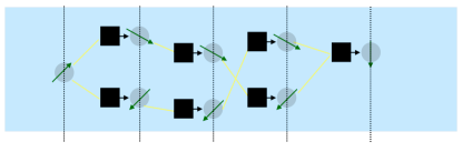
    Figure 20: More extended loop
  • Contributions of two, three-loops,… can be considered similarly. First one can see that the probability to close two, three loops… scales as $O(c/N)^{2}$,$O(c/N)^{3}$,… By associating two replicas to such diagrams we find contributions to $-\beta\tilde{F}_{n,p}/(NM)$ of order $O(c/N)^{2}$,$O(c/N)^{3}$,…

  • Note that loop corrections breaks the symmetry with respect to the exchange of input/output sides.

  • In general, by associating more replicas to the same diagram we find contributions which vanish more rapidly increasing $c$.

B.5 Summary 2

Now we can collect the above results to obtain the free-energy functional $-\beta F_{n}[\hat{Q},\hat{q}]$ defined in sec. B.3,

$$\frac{-\beta F_{n}[\{\hat{Q},\hat{q}\}]}{M}=\frac{1}{\alpha}\sum_{l=1,2,\ldots,L}\sum_{\blacksquare\in l}s_{\rm ent,bond}[\hat{Q}_{\blacksquare}]+\sum_{l=1,2,\ldots,L-1}\sum_{\blacksquare\in l}s_{\rm ent,spin}[\hat{q}_{\blacksquare}]+\frac{-\beta F_{\rm ex}[\{\hat{Q}_{\blacksquare},\hat{q}_{\blacksquare}\}]}{M}$$ (100)

with the first two terms being the entropic part of the free-energy due to bonds and spins (see Eq. (73) and Eq. (79)),

$\displaystyle cs_{\rm ent,bond}[\hat{Q}]$ $\displaystyle=$ $\displaystyle-\beta G_{n,0}^{\rm bond}[\hat{\epsilon}_{0}^{*}]+c\sum_{a<b}(\epsilon^{*}_{0})_{ab}Q_{ab}$
$\displaystyle Ms_{\rm ent,spin}[\hat{Q}]$ $\displaystyle=$ $\displaystyle-\beta G_{n,0}^{\rm spin}[\hat{\epsilon}_{0}^{*}]+M\sum_{a<b}(\varepsilon^{*}_{0})_{ab}q_{ab}$ (101)

The last term in Eq. (100) is the interaction part of the free-energy $-\beta F_{\rm ex}[\{\hat{Q}_{\blacksquare},\hat{q}_{\blacksquare}\}]$ (see Eq. (87)).

In the dense limit $\lim_{c\rightarrow\infty}\lim_{N\rightarrow\infty}$, we have found that only the 1st order term $-\beta\tilde{F}_{n,1}$ (see Eq. (90)) in the Plefka expansion contributes to $-\beta\tilde{F}_{\rm ex}[\hat{Q},\hat{q},\{\partial/\partial_{\mu,\blacksquare,a}\}]$. Thus we find,

$$\frac{-\beta F_{\rm ex}[\{\hat{Q}_{\blacksquare},\hat{q}_{\blacksquare}\}]}{M}=\sum_{l=1,2,\ldots,L-1}\sum_{\blacksquare\in l}(-{\cal F}_{\rm int})\left[\hat{\lambda}_{\blacksquare}\right]$$ (102)

with

$$-{\cal F}_{\rm int}[\hat{\Lambda}]=\ln\left.\exp\left[\sum_{a,b}\Lambda_{ab}\frac{\partial^{2}}{\partial h_{a}\partial h_{b}}\right]\prod_{a}e^{-\beta v(h_{a})}\right|_{h=0}$$ (103)

and

$$\lambda_{ab,\blacksquare}=Q_{ab,\blacksquare}q_{ab,\blacksquare}\frac{1}{c}\sum_{k=1}^{c}q_{ab,\blacksquare(k)}$$ (104)

On the boundaries we have $q_{ab,\blacksquare}=q_{ab,\blacksquare}=1$ for $\blacksquare\in 0$ and $\blacksquare\in L$.

Finally, assuming that order parameters are homogeneous within the layers Eq. (19) we find the expression Eq. (24).

The saddle point equations are

$\displaystyle 0=\frac{\partial}{\partial Q_{ab,\blacksquare}}(-\beta F_{n}[\{\hat{Q},\hat{q}\}])$ $\displaystyle=$ $\displaystyle\frac{1}{\alpha}\frac{\partial}{\partial Q_{ab,\blacksquare}}{s}_{\rm ent,bond}[\hat{Q}_{\blacksquare}]+\sum_{\square}\frac{\partial\Lambda_{\square}}{\partial Q_{ab,\blacksquare}}(-{\cal F}_{\rm int})^{\prime}\left[\Lambda_{\square}\right]$
$\displaystyle 0=\frac{\partial}{\partial q_{ab,\blacksquare}}(-\beta F_{n}[\{\hat{Q},\hat{q}\}])$ $\displaystyle=$ $\displaystyle\frac{1}{\alpha}\frac{\partial}{\partial Q_{ab,\blacksquare}}{s}_{\rm ent,bond}[\hat{Q}_{\blacksquare}]+\sum_{\square}\frac{\partial\Lambda_{\square}}{\partial q_{ab,\blacksquare}}(-{\cal F}_{\rm int})^{\prime}\left[\Lambda_{\square}\right]$ (105)

B.6 Franz-Parisi’s potential in the replica symmetric ansatz

Here we display the expressions for the Franz-Parisi’s potential within the replica symmetric ansatz needed to evaluate the generalization error.

From (128) of Yoshino (2020) we find,

$\displaystyle s_{\rm ent,spin}[\hat{\epsilon}^{1+s},\hat{q}^{1+s}]=s\epsilon_{r}r+\frac{1}{2}\epsilon_{r}+\frac{s}{2}\sum_{i=0}^{k}\epsilon_{i}q_{i}(m_{i}-m_{i+1})+\frac{s}{2}\epsilon_{k}$
$\displaystyle\hskip 28.45274pt+\ln\exp\left[\frac{\Lambda^{\rm Ising}_{\rm com}}{2}\sum_{a,b=0}^{s}\frac{\partial^{2}}{\partial h_{a}\partial h_{b}}\right]\prod_{i=0}^{k}\left.\exp\left[\frac{\Lambda^{\rm Ising}_{i}}{2}\sum_{a,b=1}^{s}I_{ab}^{m_{i}}\frac{\partial^{2}}{\partial h_{a}\partial h_{b}}\right]\prod_{a=0}^{s}(2\cosh(h_{a}))\right|_{\{h_{a}=0\}}$
$\displaystyle\hskip 28.45274pt=s\epsilon_{r}r+\frac{1}{2}\epsilon_{r}+\frac{s}{2}\sum_{i=0}^{k}\epsilon_{i}q_{i}(m_{i}-m_{i+1})+\frac{s}{2}\epsilon_{k}$
$\displaystyle\hskip 56.9055pt+\left.\ln\gamma_{\Lambda_{\rm com}}\otimes(2\cosh(h)\gamma_{\Lambda_{0}^{\rm Ising}}\otimes e^{-sf^{\rm Ising}(m_{1},h)}\right|_{h=0}\qquad$ (106)

Then we find

$\displaystyle\partial_{s}\left.s_{\rm ent,spin}[\hat{\epsilon}^{1+s},\hat{q}^{1+s}]\right|_{s=0}$ $\displaystyle=$ $\displaystyle\epsilon_{r}r+\frac{1}{2}\sum_{i=0}^{k}\epsilon_{i}q_{i}(m_{i}-m_{i+1})+\frac{1}{2}\epsilon_{k}$ (107)
$\displaystyle+$ $\displaystyle\frac{\int Dz_{\rm com}\left(2\cosh(\sqrt{\Lambda_{\rm com}}z_{\rm com}\right)\int Dz_{0}(-f^{\rm Ising}(m_{1},\sqrt{\Lambda_{\rm com}}z_{\rm com}+\sqrt{\Lambda^{\rm Ising}_{0}}z_{0}))}{\int Dz_{\rm com}\left(2\cosh(\sqrt{\Lambda_{\rm com}}z_{\rm com}\right)}$

For the interaction part of the free-energy we find from (134) of Yoshino (2020),

$\displaystyle\left.-\partial_{s}{\cal F}_{\rm int}[\hat{q}^{1+s}(l-1),\hat{Q}^{1+s}(l),\hat{q}^{1+s}(l)]\right|_{s=0}=-\partial_{s}\ln\exp\left[\frac{\Lambda_{\rm com}(l)}{2}\sum_{a,b=0}^{s}\frac{\partial^{2}}{\partial h_{a}\partial h_{b}}\right]\exp\left[\frac{\Lambda_{\rm teacher}(l)}{2}\frac{\partial^{2}}{\partial h^{2}_{0}}\right]$
$\displaystyle\left.\prod_{i=0}^{k+1}\left.\exp\left[\frac{\Lambda_{i}(l)}{2}\sum_{a,b=1}^{s}I_{ab}^{m_{i}}\frac{\partial^{2}}{\partial h_{a}\partial h_{b}}\right]\prod_{a=0}^{s}e^{-\beta v(r(h_{a}))}\right|_{\{h_{a}=0\}}\right|_{s=0}$
$\displaystyle=-\partial_{s}\ln\int Dz_{\rm com}\int Dz_{\rm teacher}e^{-\beta v(\sqrt{\Lambda_{\rm com}(l)}z_{\rm com}+\sqrt{\Lambda_{\rm teacher}(l)}z_{\rm teacher})}$
$\displaystyle\left.\hskip 56.9055pt\int Dz_{0}e^{-sf(m_{1},\sqrt{\Lambda_{\rm com}(l)}z_{\rm com}+\sqrt{\Lambda_{0}(l)}z_{0})}\right|_{s=0}$
$\displaystyle=\frac{\int Dz_{\rm com}g_{\rm teacher}(\sqrt{\Lambda_{\rm com}(l)}z_{\rm com})\int Dz_{0}(-f(m_{1},\sqrt{\Lambda_{\rm com}(l)}z_{\rm com}+\sqrt{\Lambda_{0}(l)}z_{0}))}{\int Dz_{\rm com}g_{\rm teacher}(\sqrt{\Lambda_{\rm com}(l)}z_{\rm com})}$ (108)

where we introduced (see (147) of Yoshino (2020)),

$$g_{\rm teacher}(h)\equiv\int Dz_{\rm teacher}e^{-\beta v(h-\sqrt{\Lambda_{\rm teacher}}z_{\rm teacher})}$$ (109)

B.7 Quadratic and cubic expansions of the free-energy

Here expansion of the free-energy functional given by Eq. (100) supplemented by Eq. (102), Eq. (103) and Eq. (104) around the saddle point given by Eq. (105). We can write

$$Q_{ab,\blacksquare}=Q^{*}_{ab}(l)+\Delta Q_{ab,\blacksquare}\qquad q_{ab,\blacksquare}=q^{*}_{ab}(l)+\Delta q_{ab,\blacksquare}$$ (110)

where $Q^{*}_{ab}(l)$ and $q^{*}_{ab}(l)$ are the saddle point values of the order parameters, $l$ is the label of the layer to which $\blacksquare$ belongs to, $\Delta Q_{ab,\blacksquare}$ and $\Delta q_{ab,\blacksquare}$ are fluctuations around the saddle point.

B.7.1 Quadratic expansion

The quadratic expansion of the replicated free-energy functional is specified in the Hessian matrix. It is obtained as,

$\displaystyle H^{QQ}_{ab,cd,\blacksquare_{1},\blacksquare_{2}}$ $\displaystyle=$ $\displaystyle\frac{\partial^{2}}{\partial Q_{ab,\blacksquare_{1}}\partial Q_{cd,\blacksquare_{2}}}\frac{(\beta F_{n})[\{\hat{Q},\hat{q}\}]}{M}=-\delta_{\blacksquare_{1},\blacksquare_{2}}\frac{1}{\alpha}\frac{\partial^{2}}{\partial Q^{2}_{ab,\blacksquare_{1}}}{s}_{\rm ent,bond}[\hat{Q}_{\blacksquare_{1}}]$
$\displaystyle-$ $\displaystyle\sum_{\square}\frac{\partial^{2}\Lambda_{\square}}{\partial Q_{ab,\blacksquare_{1}}\partial Q_{ab,\blacksquare_{2}}}(-{\cal F}_{\rm int})^{\prime}\left[\Lambda_{\square}\right]-\sum_{\square}\frac{\partial\Lambda_{\square}}{\partial Q_{ab,\blacksquare_{1}}}\frac{\partial\Lambda_{\square}}{\partial Q_{ab,\blacksquare_{2}}}(-{\cal F}_{\rm int})^{\prime\prime}\left[\Lambda_{\square}\right]$
$\displaystyle=$ $\displaystyle-\delta_{\blacksquare_{1},\blacksquare_{2}}\left[\frac{1}{\alpha}\frac{\partial^{2}}{\partial Q^{2}_{ab,\blacksquare_{1}}}{s}_{\rm ent,bond}[\hat{Q}_{\blacksquare_{1}}]+\frac{\partial^{2}\Lambda_{\blacksquare_{1}}}{\partial Q^{2}_{ab,\blacksquare_{1}}}(-{\cal F}_{\rm int})^{\prime}\left[\Lambda_{\blacksquare_{1}}\right]+\left(\frac{\partial\Lambda_{\blacksquare_{1}}}{\partial Q_{ab,\blacksquare_{1}}}\right)^{2}(-{\cal F}_{\rm int})^{\prime\prime}\left[\Lambda_{\blacksquare_{1}}\right]\right]$
$\displaystyle H^{Qq}_{ab,cd,\blacksquare_{1},\blacksquare_{2}}$ $\displaystyle=$ $\displaystyle\frac{\partial^{2}}{\partial Q_{ab,\blacksquare_{1}}\partial q_{cd,\blacksquare_{2}}}\frac{(\beta F)[\{\hat{Q},\hat{q}\}]}{M}$
$\displaystyle=$ $\displaystyle-\sum_{\square}\frac{\partial^{2}\Lambda_{\square}}{\partial Q_{ab,\blacksquare_{1}}\partial q_{ab,\blacksquare_{2}}}(-{\cal F}_{\rm int})^{\prime}\left[\Lambda_{\square}\right]-\sum_{\square}\frac{\partial\Lambda_{\square}}{\partial Q_{ab,\blacksquare_{1}}}\frac{\partial\Lambda_{\square}}{\partial q_{ab,\blacksquare_{2}}}(-{\cal F}_{\rm int})^{\prime\prime}\left[\Lambda_{\square}\right]$
$\displaystyle=$ $\displaystyle-\frac{\partial^{2}\Lambda_{\blacksquare_{1}}}{\partial Q_{ab,\blacksquare_{1}}\partial q_{ab,\blacksquare_{2}}}(-{\cal F}_{\rm int})^{\prime}\left[\Lambda_{\blacksquare_{1}}\right]-\frac{\partial\Lambda_{\blacksquare_{1}}}{\partial Q_{ab,\blacksquare_{1}}}\frac{\partial\Lambda_{\blacksquare_{1}}}{\partial q_{ab,\blacksquare_{2}}}(-{\cal F}_{\rm int})^{\prime\prime}\left[\Lambda_{\blacksquare_{1}}\right]$
$\displaystyle H^{qq}_{ab,cd,\blacksquare_{1},\blacksquare_{2}}$ $\displaystyle=$ $\displaystyle\frac{\partial^{2}}{\partial q_{ab,\blacksquare}\partial q_{cd,\square}}\frac{(\beta F)[\{\hat{Q},\hat{q}\}]}{M}=-\delta_{\blacksquare_{1},\blacksquare_{2}}\frac{\partial^{2}}{\partial q^{2}_{ab,\blacksquare_{1}}}{s}_{\rm ent,spin}[\hat{q}_{\blacksquare_{1}}]$ (111)
$\displaystyle-$ $\displaystyle\sum_{\square}\frac{\partial^{2}\Lambda_{\square}}{\partial q_{ab,\blacksquare_{1}}\partial q_{ab,\blacksquare_{2}}}(-{\cal F}_{\rm int})^{\prime}\left[\Lambda_{\square}\right]-\sum_{\square}\frac{\partial\Lambda_{\square}}{\partial q_{ab,\blacksquare_{1}}}\frac{\partial\Lambda_{\square}}{\partial q_{ab,\blacksquare_{2}}}(-{\cal F}_{\rm int})^{\prime\prime}\left[\Lambda_{\square}\right]$

where

$\displaystyle\frac{\partial\Lambda_{\blacksquare_{1}}}{\partial Q_{ab,\blacksquare_{1}}}=q_{ab,\blacksquare_{1}}\frac{1}{c}\sum_{k=1}^{c}q_{ab,\blacksquare_{1}(k)}\qquad\frac{\partial^{2}\Lambda_{\blacksquare_{1}}}{\partial Q^{2}_{ab,\blacksquare_{1}}}=0$ (112)

and

$\displaystyle\frac{\partial^{2}\Lambda_{\blacksquare_{1}}}{\partial Q_{ab,\blacksquare_{1}}\partial q_{ab,\blacksquare_{2}}}$ $\displaystyle=$ $\displaystyle\delta_{\blacksquare_{1},\blacksquare_{2}}\frac{1}{c}\sum_{k=1}^{c}q_{ab,\blacksquare_{1}(k)}+\frac{1}{c}q_{ab,\blacksquare_{1}}I_{\partial\blacksquare_{1}}(\blacksquare_{2})$
$\displaystyle\frac{\partial\Lambda_{\blacksquare_{1}}}{\partial Q_{ab,\blacksquare_{1}}}\frac{\partial\Lambda_{\blacksquare_{1}}}{\partial q_{ab,\blacksquare_{2}}}$ $\displaystyle=$ $\displaystyle\delta_{\blacksquare_{1},\blacksquare_{2}}q_{ab,\blacksquare_{1}}Q_{ab,\blacksquare_{1}}\left(\frac{1}{c}\sum_{k=1}^{c}q_{ab,\blacksquare_{1}(k)}\right)^{2}+\frac{1}{c}q^{2}_{ab,\blacksquare_{1}}Q_{ab,\blacksquare_{1}}\left(\frac{1}{c}\sum_{k=1}^{c}q_{ab,\blacksquare_{1}(k)}\right)I_{\partial\blacksquare_{1}}(\blacksquare_{2})$ (113)

and

$\displaystyle\sum_{\square}\frac{\partial^{2}\Lambda_{\square}}{\partial q_{ab,\blacksquare_{1}}\partial q_{ab,\blacksquare_{2}}}$ $\displaystyle=$ $\displaystyle\frac{1}{c}\left(Q_{ab,\blacksquare_{1}}I_{\partial\blacksquare_{1}}(\blacksquare_{2})+Q_{ab,\blacksquare_{2}}I_{\partial\blacksquare_{2}}(\blacksquare_{1})\right)$
$\displaystyle\sum_{\square}\frac{\partial\Lambda_{\square}}{\partial q_{ab,\blacksquare_{1}}}\frac{\partial\Lambda_{\square}}{\partial q_{ab,\blacksquare_{2}}}$ $\displaystyle=$ $\displaystyle\delta_{\blacksquare_{1},\blacksquare_{2}}\left(Q_{ab,\blacksquare_{1}}\frac{1}{c}\sum_{k=1}^{c}q_{ab,\blacksquare_{1}(k)}\right)^{2}$ (114)
$\displaystyle+\frac{1}{c}Q^{2}_{ab,\blacksquare_{1}}q_{ab,\blacksquare_{1}}\frac{1}{c}\sum_{k=1}^{c}q_{ab,\blacksquare_{1}(k)}I_{\partial\blacksquare_{1}}(\blacksquare_{2})+\frac{1}{c}Q^{2}_{ab,\blacksquare_{2}}q_{ab,\blacksquare_{2}}\frac{1}{c}\sum_{k=1}^{c}q_{ab,\blacksquare_{2}(k)}I_{\partial\blacksquare_{2}}(\blacksquare_{1})$
$\displaystyle+$ $\displaystyle\frac{1}{c^{2}}\sum_{\square}\left(q_{ab,\square}Q_{ab,\square}\right)^{2}I_{\partial\square}(\blacksquare_{1})I_{\partial\square}(\blacksquare_{2})$

where $I_{A}(x)$ is the indicator function, i. e. $I_{a}(x)=1$ if $x\in a$ and 00 otherwise.

Let us note that in the liquid phase where $Q_{ab}=q_{ab}=0$ for $a\neq b$, the Hessian matrix become simplified as,

$\displaystyle H^{QQ}_{ab,cd,\blacksquare_{1},\blacksquare_{2}}$ $\displaystyle=$ $\displaystyle-\delta_{\blacksquare_{1},\blacksquare_{2}}\left.\frac{1}{\alpha}\frac{\partial^{2}}{\partial Q_{ab,\blacksquare_{1}}\partial Q_{cd,\blacksquare_{1}}}s_{\rm ent,bond}[\hat{Q}_{\blacksquare_{1}}]\right|_{\hat{Q}_{\blacksquare_{1}}=0}$
$\displaystyle H^{Qq}_{ab,cd,\blacksquare_{1},\blacksquare_{2}}$ $\displaystyle=$ $\displaystyle 0$
$\displaystyle H^{qq}_{ab,cd,\blacksquare_{1},\blacksquare_{2}}$ $\displaystyle=$ $\displaystyle-\delta_{\blacksquare_{1},\blacksquare_{2}}\left.\frac{\partial^{2}}{\partial q_{ab,\blacksquare_{1}}\partial q_{cd,\blacksquare_{1}}}s_{\rm ent,spin}[\hat{q}_{\blacksquare_{1}}]\right|_{\hat{q}_{\blacksquare_{1}}=0}$ (115)

B.7.2 Cubic expansion

Here let us analyze the cubic expansion. For simplicity let us only consider the liquid phase where $Q_{ab}=q_{ab}=0$ for $a\neq b$. We find the only non-vanishing contribution is due to,

$\displaystyle W^{qQq}_{ab,cd,ef,\blacksquare_{1},\blacksquare_{2},\blacksquare_{3}}$ $\displaystyle=$ $\displaystyle\left.\frac{\partial^{3}}{\partial q_{ab,\blacksquare_{1}}\partial Q_{cd,\blacksquare_{2}}\partial_{ef,\blacksquare_{3}}}\frac{(\beta F_{n})[\{\hat{Q},\hat{q}\}]}{M}\right|_{\hat{Q}=\hat{q}=0}$ (116)
$\displaystyle=$ $\displaystyle\left.-\frac{\partial^{3}\Lambda_{\blacksquare_{2}}}{\partial q_{ab,\blacksquare_{1}}\partial Q_{ab,\blacksquare_{2}}\partial q_{ab,\blacksquare_{3}}}(-{\cal F}_{\rm int})^{\prime}\left[\Lambda_{\blacksquare_{2}}\right]\right|_{\hat{Q}=\hat{q}=0}\delta_{(ab),(cd)}\delta_{(cd),(ef)}$
$\displaystyle=$ $\displaystyle-\frac{1}{c}\left[I_{\partial\blacksquare_{2}}(\blacksquare_{1})\delta_{\blacksquare_{2},\blacksquare_{3}}+\delta_{\blacksquare_{2},\blacksquare_{1}}I_{\partial\blacksquare_{2}}(\blacksquare_{3})\right]\left.(-{\cal F}_{\rm int})^{\prime}\left[\Lambda_{\blacksquare_{2}}\right]\right|_{\hat{Q}=\hat{q}=0}\delta_{(ab),(cd)}\delta_{(cd),(ef)}$

It is interesting to note that this cubic term breaks the symmetry concerning the exchange of input/output sides.

B.7.3 Correction to the saddle point

Now let us turn to corrections due to fluctuations around the saddle point. These give finite connectivity $c$ or $M=c\alpha$ corrections ($\alpha$ is fixed).

We can write

$$Q_{ab,\blacksquare}=Q^{*}_{ab}(l)+\Delta Q_{ab,\blacksquare}\qquad q_{ab,\blacksquare}=q^{*}_{ab}(l)+\Delta Q_{ab,\blacksquare}$$ (117)

where $Q^{*}_{ab}(l)$ and $q^{*}_{ab}(l)$ are the saddle point values of the order parameters, $l$ is the label of the layer to which $\blacksquare$ belongs to, $\Delta Q_{ab,\blacksquare}$ and $\Delta q_{ab,\blacksquare}$ are fluctuations around the saddle point. Including the correction due to the fluctuations around the saddle point, the replicated Gardner volume Eq. (21) can be written as,

$$\overline{V^{1+s}({\bf S}_{0},{\bf S}_{L}({\bf S}_{0},{\cal J}_{\rm teacher})))}^{{\bf S}_{0},{\cal J}_{\rm teacher}}=e^{NMs_{1+s}[\{{\hat{Q}}^{*},{\hat{q}}^{*}\}]}Z_{\rm fluctuation}$$ (118)

where

$\displaystyle Z_{\rm fluctuation}$ $\displaystyle=$ $\displaystyle\int\prod_{\blacksquare}\prod_{a<b}d\Delta Q_{ab,\blacksquare}d\Delta q_{ab,\blacksquare}\exp\left[-\frac{M}{2}\sum_{a<b}\sum_{c<d}\sum_{\blacksquare,\square}[H^{QQ}_{ab,cd,\blacksquare,\square}\Delta Q_{ab,\blacksquare}\Delta Q_{cd,\square}\right.$ (119)
$\displaystyle\left.\left.+H^{Qq}_{ab,cd,\blacksquare,\square}\Delta Q_{ab,\blacksquare}\Delta q_{cd,\square}+H^{qq}_{ab,cd,\blacksquare,\square}\Delta q_{ab,\blacksquare}\Delta q_{cd,\square}\right]\right.$
$\displaystyle\left.\left.-\frac{M}{3!}\sum_{a<b}\sum_{c<d}\sum_{e<f}\sum_{\blacksquare_{1},\blacksquare_{2},\blacksquare_{3}}\left[W_{ab,cd,ef,\blacksquare_{1},\blacksquare_{2},\blacksquare_{3}}^{qQq}\Delta q_{ab,\blacksquare_{1}}\Delta Q_{cd,\blacksquare_{2}}\Delta q_{ef,\blacksquare_{3}}+\ldots\right]\right]\right]$

where $H^{QQ}_{ab,cd,\blacksquare,\square}...$ are the Hessian matrices given in sec. B.7.

For the following discussion, we do not need to perform a complete analysis of the correction. We restrict ourselves in the liquid phase $Q=q=0$. Then as shown in sec. B.7, the Hessian matrices become completely local, i. e. $H^{QQ}_{\blacksquare,\square}=\delta_{\blacksquare,\square}H^{QQ}_{\blacksquare,\blacksquare}$ and $H^{qq}_{\blacksquare,\square}=\delta_{\blacksquare,\square}H^{qq}_{\blacksquare,\blacksquare}$ while $H^{Qq}_{\blacksquare,\square}=0$ (see Eq. (115)). Thus at the quadratic level of fluctuations, there is no correlation between different layers in the liquid phase. In the cubic order, we find $W^{qQq}_{\blacksquare_{1},\blacksquare_{2},\blacksquare_{3}}\propto\frac{1}{c}\left[I_{\partial\blacksquare_{2}}(\blacksquare_{1})\delta_{\blacksquare_{2},\blacksquare_{3}}+\delta_{\blacksquare_{2},\blacksquare_{1}}I_{\partial\blacksquare_{2}}(\blacksquare_{3})\right]$ (see Eq. (116)). This will induce correlations between different layers even in the liquid phase. And this will be enhanced next to the frozen wall and enhanced by correlation in the frozen wall (the hidden manifold model).

To understand the key point it is sufficient to consider a simplified model.

$$Z=\int\prod_{\blacksquare}dx_{\blacksquare}dy_{\blacksquare}\exp\left[-\frac{M}{2}\sum_{\blacksquare}h_{xx}x_{\blacksquare}^{2}-\frac{M}{2}\sum_{\blacksquare}h_{yy}y_{\blacksquare}^{2}-\alpha w\sum_{\blacksquare}\sum_{\square\in\partial\blacksquare}y_{\blacksquare}x_{\blacksquare}y_{\square}\right]$$ (120)

Then by introducing

$$Z_{0}=\int\prod_{\blacksquare\in(1,2,\ldots,L)}dx_{\blacksquare}\exp\left[-\frac{M}{2}\sum_{\blacksquare}h_{xx}x_{\blacksquare}^{2}\right]\int\prod_{\blacksquare\in(1,2,\ldots,L-1)}dy_{\blacksquare}\exp\left[-\frac{M}{2}\sum_{\blacksquare}h_{yy}y_{\blacksquare}^{2}\right]=\left(\sqrt{\frac{2\pi}{Mh_{xx}}}\right)^{NL}\left(\sqrt{\frac{2\pi}{Mh_{yy}}}\right)^{N(L-1)}$$ (121)

and

$$\langle\cdots\rangle_{x,y}=\frac{\int\prod_{\blacksquare}dx_{\blacksquare}\prod_{\blacksquare}dy_{\blacksquare}\exp\left[-M\frac{h_{xx}}{2}\sum_{\blacksquare}x_{\blacksquare}^{2}-M\frac{h_{yy}}{2}\sum_{\blacksquare}y_{\blacksquare}^{2}\right]\ldots}{\int\prod_{\blacksquare}dx_{\blacksquare}\prod_{\blacksquare}dy_{\blacksquare}\exp\left[-M\frac{h_{xx}}{2}\sum_{\blacksquare}x_{\blacksquare}^{2}-M\frac{h_{yy}}{2}\sum_{\blacksquare}y_{\blacksquare}^{2}\right]}$$ (122)

we can write

$\displaystyle\ln Z-\ln Z_{0}$ $\displaystyle=$ $\displaystyle\ln\left\langle\exp\left[-\alpha w\sum_{\blacksquare}\sum_{\square\in\partial\blacksquare}y_{\blacksquare}x_{\blacksquare}y_{\square}\right]\right\rangle_{x}$ (123)
$\displaystyle=$ $\displaystyle-\alpha w\sum_{\blacksquare}\sum_{\square\in\partial\blacksquare}\langle y_{\blacksquare}x_{\blacksquare}y_{\square}\rangle_{xy}+\frac{1}{2}\left(\alpha w\right)^{2}\sum_{\blacksquare_{1}}\sum_{\square_{1}\in\partial\blacksquare_{1}}\sum_{\blacksquare_{2}}\sum_{\square_{2}\in\partial\blacksquare_{2}}\langle y_{\blacksquare_{1}}x_{\blacksquare_{1}}y_{\square_{1}}y_{\blacksquare_{2}}x_{\blacksquare_{2}}y_{\square_{2}}]\rangle_{xy}+\ldots$
$\displaystyle=$ $\displaystyle\frac{1}{2}\left(\alpha w\right)^{2}\sum_{\blacksquare}\sum_{\square\in\partial\blacksquare}\langle\underbrace{y^{2}_{\blacksquare}x^{2}_{\blacksquare}y^{2}_{\square}}_{M^{3}(h_{yy}h_{xx}h_{yy})^{-1}}\rangle_{xy}+\ldots$

References