Quantum Learning Theory Beyond Batch Binary Classification

Abstract

Arunachalam and de Wolf (2018) showed that the sample complexity of quantum batch learning of boolean functions, in the realizable and agnostic settings, has the same form and order as the corresponding classical sample complexities. In this paper, we extend this, ostensibly surprising, message to batch multiclass learning, online boolean learning, and online multiclass learning. For our online learning results, we first consider an adaptive adversary variant of the classical model of Dawid and Tewari (2022). Then, we introduce the first (to the best of our knowledge) model of online learning with quantum examples.

1 Introduction

Ever since Bshouty and Jackson (1995)’s formalization of a quantum example, several works (Servedio and Gortler, 2004; Atici and Servedio, 2005; Zhang, 2010), culminating in Arunachalam and de Wolf (2018), have provided sample complexity bounds for quantum batch learning of boolean functions. In Arunachalam and de Wolf (2018), the message was crystallized:

1. There is no new combinatorial dimension needed to characterize quantum batch learnability of boolean functions, namely the VC dimension continues to do so.

2. There is at most a constant sample complexity advantage for quantum batch learning of boolean functions, in both the realizable and agnostic settings, as compared to the corresponding classical sample complexities.

In this paper, we show that this message continues to hold in three other learning settings: batch learning of multiclass functions, online learning of boolean functions, and online learning of multiclass functions.

Our motivation for considering quantum batch learning of multiclass functions is an open question in Arunachalam and de Wolf (2018) which asks “what is the quantum sample complexity for learning concepts whose range is $[k]$ rather than $\{0,1\}$, for some $k>2$?” We resolve this question for $2<k<\infty$ (see Section 3). In classical multiclass batch learning, an approach to establish the lower and upper sample complexity bounds (Daniely et al., 2015) is to proceed via a reduction to the binary case, with an appeal to the definition of Natarajan dimension. While classically straightforward, extending such a proof approach to establish sample complexity bounds for quantum multiclass batch learning involves manipulating quantum examples, which has to be done with utmost care (see Section 3.2.1).

Unlike the batch setting, quantum online learning of classical functions, to the best of our knowledge, has no predefined model. One possible explanation is that we need, as an intermediary, a new classical online learning model (see Sections 4.2, 4.3) where, at each round, the adversary provides a distribution over the example (input-label) space instead of a single example. With this new classical model, and the definition of a quantum example, a model for online learning in the quantum setting arises as a natural extension (see Figure 1).

Figure 1: Mapping of the tools necessary for generalizations of learning paradigms from classical to quantum.

1.1 Our Contributions

In Tables 1 and 2, we provide a concise overview of existing results and highlight our contributions in batch and online learning for binary and multiclass classification across realizable and agnostic settings in both classical and quantum paradigms. Our contributions include:

• establishing lower and upper sample complexity bounds for quantum batch multiclass classification in the realizable and agnostic settings,

• proposing a new classical online learning model, which is an adaptive adversary variant of an existing classical online learning model (Dawid and Tewari, 2022),

• proposing a quantum online learning model, as a natural generalization of our proposed classical online learning model,

• establishing tight expected regret bounds for quantum online binary classification in the realizable and agnostic settings,

• establishing a tight expected regret bound for quantum online multiclass classification in the realizable setting, and

• establishing lower and upper expected regret bounds for quantum online multiclass classification in the agnostic setting.

Notes on Tables 1 and 2

• In all cases, we state known results that exhibit the tightest dependence on the combinatorial parameters that characterize learning in the respective settings.

• In the batch multiclass case, we work with Natarajan dimension, instead of DS dimension which was shown to characterize classical batch multiclass learning (including the $k\to\infty$ case) recently (Brukhim et al., 2022). We defer the resolution of the quantum sample complexity in the $k\to\infty$ case to future work.

• In the batch multiclass realizable case, there exists an upper bound with a tighter dependence on $\epsilon$ (but looser on $\text{Ndim}({\mathcal{H}})$) for both classical and quantum cases (see Section 3.2.2).

• In the (canonical) classical online multiclass agnostic case, the $\tilde{\mathcal{O}}(\sqrt{\text{mcLdim}({\mathcal{H}})T})$ bound hides $\sqrt{\log\Big{(}\frac{T}{\text{mcLdim}({\mathcal{H}})}\Big{)}}$ factors (Hanneke et al., 2023).

• The definition of loss/regret differs between the canonical classical adversary-provides-an-input model (in Section 4.1) and both the classical adversary-provides-a-distribution model (in Sections 4.2, 4.3) and the quantum online model (in Section 5). Specifically, the former employs the indicator loss (mistake model), whereas the latter two involve probabilistic losses.

		Classical	Quantum
Boolean	Realizable	$\Theta\Big{(}\frac{\text{VCdim}({\mathcal{H}})+\log(\frac{1}{\delta})}{\epsilon}\Big{)}$	$\Theta\Big{(}\frac{\text{VCdim}({\mathcal{H}})+\log(\frac{1}{\delta})}{\epsilon}\Big{)}$
		Blumer et al. (1989); Hanneke (2016)	Arunachalam and de Wolf (2018)
	Agnostic	$\Theta\Big{(}\frac{\text{VCdim}({\mathcal{H}})+\log(\frac{1}{\delta})}{\epsilon^{2}}\Big{)}$	$\Theta\Big{(}\frac{\text{VCdim}({\mathcal{H}})+\log(\frac{1}{\delta})}{\epsilon^{2}}\Big{)}$
		Kearns et al. (1992); Talagrand (1994)	Arunachalam and de Wolf (2018)
Multiclass	Realizable	$\Omega\Big{(}\frac{\text{Ndim}({\mathcal{H}})+\log(\frac{1}{\delta})}{\epsilon}\Big{)}$	$\Omega\Big{(}\frac{\text{Ndim}({\mathcal{H}})+\log(\frac{1}{\delta})}{\epsilon}\Big{)}$
		Natarajan (1989)	(Thm. 3.3)
		$\mathcal{O}\Big{(}\frac{\text{Ndim}({\mathcal{H}})\log(k)\log(\frac{1}{\epsilon})+\log(\frac{1}{\delta})}{\epsilon}\Big{)}$	$\mathcal{O}\Big{(}\frac{\text{Ndim}({\mathcal{H}})\log(k)\log(\frac{1}{\epsilon})+\log(\frac{1}{\delta})}{\epsilon}\Big{)}$
		Daniely et al. (2015)	(Thm. 3.8)
	Agnostic	$\Omega\Big{(}\frac{\text{Ndim}({\mathcal{H}})+\log(\frac{1}{\delta})}{\epsilon^{2}}\Big{)}$,	$\Omega\Big{(}\frac{\text{Ndim}({\mathcal{H}})+\log(\frac{1}{\delta})}{\epsilon^{2}}\Big{)}$ (Thm. 3.3)
		$\mathcal{O}\Big{(}\frac{\text{Ndim}({\mathcal{H}})\log(k)+\log(\frac{1}{\delta})}{\epsilon^{2}}\Big{)}$	$\mathcal{O}\Big{(}\frac{\text{Ndim}({\mathcal{H}})\log(k)+\log(\frac{1}{\delta})}{\epsilon^{2}}\Big{)}$
		Ben-David et al. (1995)	(Thm. 3.8)

Table 1: An overview of sample complexity results for batch learning in classical and quantum paradigms. Our novel contributions are presented in boxes shaded gray.

		Canonical Classical	Classical
		(Input-based)	(Distribution-based)	Quantum
Boolean	Realizable	$\Theta(\text{Ldim}({\mathcal{H}}))$	$\Theta({\text{Ldim}({\mathcal{H}})})$	$\Theta({\text{Ldim}({\mathcal{H}})})$
		Littlestone (1988)	(Thms. 4.6, 4.7)	(Thms. 5.4, 5.5)
	Agnostic	$\Theta(\sqrt{\text{Ldim}({\mathcal{H}})T})$	$\Theta(\sqrt{\text{Ldim}({\mathcal{H}})T})$	$\Theta(\sqrt{\text{Ldim}({\mathcal{H}})T})$
		Ben-David et al. (2009)
		Alon et al. (2021)	(Thms. 4.10, 4.11)	(Thms. 5.4, 5.5)
Multiclass	Realizable	$\Theta(\text{mcLdim}({\mathcal{H}}))$	$\Theta(\text{mcLdim}({\mathcal{H}}))$	$\Theta(\text{mcLdim}({\mathcal{H}}))$
		Daniely et al. (2015)	(Thms. 4.13, 4.14)	(Thms. 5.6, 5.7)
	Agnostic	$\Omega({\sqrt{\text{mcLdim}({\mathcal{H}})T}})$	$\Omega({\sqrt{\text{mcLdim}({\mathcal{H}})T}})$	$\Omega({\sqrt{\text{mcLdim}({\mathcal{H}})T}})$
		Daniely et al. (2015)	(Thm. 4.20)	(Thm. 5.6)
		$\tilde{\mathcal{O}}(\sqrt{\text{mcLdim}({\mathcal{H}})T})$	$\mathcal{O}(\sqrt{\text{mcLdim}({\mathcal{H}})T\log(Tk)})$	$\mathcal{O}(\sqrt{\text{mcLdim}({\mathcal{H}})T\log(Tk)})$
		Hanneke et al. (2023)	(Thm. 4.19)	(Thm. 5.7)

Table 2: An overview of expected regret bounds for online learning in the canonical classical (adversary-provides-an-input), classical adversary-provides-a-distribution, and quantum paradigms. Our novel contributions are presented in boxes shaded gray.

1.2 Organization

The paper is organized as follows. In Section 2, we present preliminaries, including notation, quantum basics, and batch learning frameworks. Section 3 contains one of our main results, addressing the quantum sample complexity in the batch multiclass setting. Moving on to Section 4, we revisit the canonical online model (Section 4.1), followed by the introduction and presentation of results for the classical adversary-provides-a-distribution model in both realizable (Section 4.2) and agnostic (Section 4.3) settings for both binary and multiclass (Section 4.4) classification. This model serves as an intermediary for transitioning from the canonical classical online model to the quantum online model. In Section 5, we introduce the quantum online learning model and summarize results within the established framework. The paper concludes with a discussion and reflection on the obtained results in Sections 5.4 and 6, along with some open questions for future exploration.

2 Preliminaries

In this section, we revisit notation, offer a brief overview of the fundamentals of quantum computing, and introduce batch learning frameworks in both classical and quantum paradigms.

2.1 Notation

In the bra-ket (Dirac) notation, a ket, $\ket{x}$, denotes a column vector in a complex vector space with an inner product (i.e. a Hilbert space). It is used primarily in the context of describing the state of a quantum system (e.g. see Definition 2.1). A bra $\bra{\cdot}$ is the dual of the ket, in that $\bra{x}=\ket{x}^{\dagger}$, where the $\dagger$ operator denotes the conjugate transpose. Typically, the bra notation is used for operators $\bra{M}$ (e.g. measurement operators) acting on a ket. This notation lends itself naturally to the notion of inner product $\braket{x}{x}=\|x\|^{2}$, and matrix-vector multiplication $\braket{M}{x}$. Furthermore, note that $\ket{x,y}$ denotes the tensor product $\ket{x}\otimes\ket{y}$, where $\otimes$ denotes the standard tensor product of two vector spaces. The comma may be omitted, and we have numerous equivalent notations for the tensor product summarized via the e.g. $\ket{0^{2}}=\ket{00}=\ket{0,0}=\ket{0}\ket{0}=\ket{0}\otimes\ket{0}=\ket{0}^{\otimes 2}$.

2.2 Quantum Basics

Analogous to how a classical bit (bit) is a unit of classical information, a quantum bit (qubit) is a unit of quantum information. The difference between the two is best illustrated by considering how each is realized. A bit is realized via the expectation value of a physical property of a system (e.g. voltage across an element in an electric circuit). If the value is higher than a certain threshold, the bit assumes the value 1. Otherwise, it assumes the value 0. Thus, a bit carries the information equivalent of its namesake, a binary digit. A qubit, on the other hand, is realized as a two-level quantum system; for e.g., as the spin (up, down) of an electron, the polarization (horizontal, vertical) of a photon, or the discrete energy levels (ground, excited) of an ion. Consequently, it is governed by the postulates of quantum mechanics (Nielsen and Chuang, 2010), as detailed in the following paragraphs.

The state space of a qubit is a 2-dimensional complex vector space, denoted as $\mathbb{C}^{2}$. The definition of a qubit as a state vector within this space is presented in the following definition.

Definition 2.1 (Qubit).

A single (isolated) qubit is described by a state vector $\ket{\psi}$, which is a unit vector in the state space $\mathbb{C}^{2}$. Mathematically,

$$\ket{\psi}=\alpha_{0}\ket{0}+\alpha_{1}\ket{1},\quad\alpha_{0},\alpha_{1}\in\mathbb{C},\quad|\alpha_{0}|^{2}+|\alpha_{1}|^{2}=1,$$

where $\ket{0}=\begin{bmatrix}1\\ 0\end{bmatrix}$ and $\ket{1}=\begin{bmatrix}0\\ 1\end{bmatrix}$ are basis vectors for the state space.

So, although we have two basis states (much as we did for the classical bit), the qubit is allowed to be in a (complex) superposition of the two, whereas a classical bit must deterministically be in one of the basis states. Additionally, as our learning examples (refer to (1), (2)) will involve multiple qubits, it is important to note that the state space of the composite system, comprising many qubits, is the tensor product of the state spaces of its components (i.e. the individual qubits); i.e. the joint state of the composite system formed by $n$ qubits, each in state $\ket{\psi_{i}},\;i\in\{1,\ldots,n\}$, is given by, $\ket{\psi_{1}}\otimes\ket{\psi_{2}}\otimes\cdots\otimes\ket{\psi_{n}}\in\mathbb{C}^{2^{n}}$. Now, let us express the state vector for multi-qubit system in terms of the standard basis elements.

Definition 2.2 (Multi-qubit system).

The state vector, $\ket{\Psi}\in\mathbb{C}^{2^{n}}$, describing the system of $n$ qubits can be expressed in terms of the standard basis elements $\{\ket{b}=\ket{b_{1}}\otimes\cdots\otimes\ket{b_{n}}|\,b=(b_{1},\ldots,b_{n})\in\{0,1\}^{n}\}$ as follows:

$$\ket{\Psi}=\sum_{b\in\{0,1\}^{n}}\alpha_{b}\ket{b},$$

where $\alpha_{b}=\braket{\Psi}{b}\in\mathbb{C}$, $\sum_{b}|\alpha_{b}|^{2}=1$.

In contrast, the joint state of $n$ classical bits is described by their Cartesian product. This essential distinction between Cartesian and tensor products is precisely the phenomenon of quantum entanglement, namely the existence of (pure) states of a composite system that are not product states of its parts. Quantum entanglement, alongside superposition, lies at the heart of intrinsic advantages of quantum computing.

Any manipulation of a quantum system is confined to unitary evolution. In the context of computation, this implies that all quantum gates are unitary operators, restricting their application to reversible computations. An avenue for irreversible computation, and the only way to obtain classical outputs in the quantum realm, is the notion of a measurement.

Definition 2.3 (Measurement).

Quantum measurements are described by a collection $\{M_{m}\}$ of measurement operators acting on the state space of the system. The index $m$ denotes the possible classical outcomes of the measurement. If the quantum system is in the state $\ket{\psi}$ before measurement, then the probability that result $m$ occurs is given by $p(m)=\bra{\psi}M_{m}^{\dagger}M_{m}\ket{\psi}$, and the state of the system after the measurement, if $m^{\star}$ is observed, “collapses to” $M_{m^{\star}}\ket{\psi}/\sqrt{p(m^{\star})}$. To ensure the conservation of total probability, $\sum_{m}M_{m}^{\dagger}M_{m}=I$ is satisfied.

Here are a couple of examples to illustrate the above definition:

• A measurement in the standard basis is implemented by measurement operators $M_{0}=\ket{0}\bra{0}$ and $M_{1}=\ket{1}\bra{1}$.

• A measurement in the standard basis of the state $\ket{\Psi}=\sum_{b\in\{0,1\}^{n}}\alpha_{b}\ket{b}$ yields the classical outcome $b$ with probability $|\alpha_{b}|^{2}$.

2.3 PAC Learning Framework

In the classical PAC (Probably Approximately Correct) learning model (Valiant, 1984), a learner is provided oracle access to samples $(x,y)$, where $x$ is sampled from some unknown distribution $D$ on ${\mathcal{X}}$ and $y=h^{\star}(x)$, for some target hypothesis $h^{\star}:{\mathcal{X}}\to{\mathcal{Y}}$. We assume that $h^{\star}\in{\mathcal{H}}$, where ${\mathcal{H}}$ is a predefined hypothesis class, i.e., the learner has prior knowledge of ${\mathcal{H}}$. The goal of the learning problem is to find $h:{\mathcal{X}}\to{\mathcal{Y}}$ such that the generalization error, given by the loss function ${\mathcal{L}}(h,D,h^{\star})=\mathds{P}_{x\sim D}(h(x)\neq h^{\star}(x))$, is minimized.

Definition 2.4 (PAC learner).

An algorithm ${\mathcal{A}}$ is an $(\epsilon,\delta)$-PAC learner for a hypothesis class ${\mathcal{H}}$ if, for any unknown distribution $D$ and for all $h^{\star}\in{\mathcal{H}}$, ${\mathcal{A}}$ takes in $m$ pairs of labeled instances, i.e., $\{(x_{i},h^{\star}(x_{i}))\}_{i=1}^{m}$, each drawn i.i.d. from $D$, and outputs a hypothesis $h$ such that $\mathds{P}[{{\mathcal{L}}(h,D,h^{\star})\leq\epsilon}]\geq 1-\delta$, where the outer probability is over the sequence of examples and the learner’s internal randomness.

Indeed, an $(\epsilon,\delta)$-PAC learner outputs a hypothesis that is, with high probability ($\geq 1-\delta$), approximately correct (${\mathcal{L}}\leq\epsilon$). A hypothesis class ${\mathcal{H}}$ is PAC-learnable if there exists an algorithm ${\mathcal{A}}$ that is an $(\epsilon,\delta)$-PAC learner for ${\mathcal{H}}$. When ${\mathcal{Y}}=\{0,1\}$, we are in the setting of binary classification. To express the sample complexity of learning boolean function classes later on, we define below a key combinatorial parameter known as the VC dimension.

Definition 2.5 (VC dimension).

Given a hypothesis class ${\mathcal{H}}=\{h:{\mathcal{X}}\to\{0,1\}\}$, a set $S=\{s_{1},\ldots,s_{t}\}\subseteq{\mathcal{X}}$ is said to be shattered by ${\mathcal{H}}$ if, for every labeling $\ell\in\{0,1\}^{t}$, there exists an $h\in{\mathcal{H}}$ such that $(h(s_{1}),h(s_{2}),\ldots,h(s_{t}))=\ell$. The VC dimension of ${\mathcal{H}}$, $\text{VCdim}({\mathcal{H}})$, is the size of the largest set $S$ that is shattered by ${\mathcal{H}}$.

2.4 Agnostic Learning Framework

In the PAC learning framework, we worked with the realizability assumption, namely that $h^{\star}\in{\mathcal{H}}$. If we omit this rather strong assumption, we are able to generalize the PAC learning framework to the agnostic learning framework (Kearns et al., 1992). Here, a learner is provided with oracle access to samples $(x,y)$, sampled from some unknown distribution $D$ on ${\mathcal{X}}\times{\mathcal{Y}}$. The learner has knowledge of a predefined hypothesis class ${\mathcal{H}}$. The objective of the learning problem is to find${}^{\ref{footnote:proper-improper}}$ $h:{\mathcal{X}}\to{\mathcal{Y}}$ such that the regret

$${\mathcal{R}}(h,D)=\mathds{P}_{(x,y)\sim D}(h(x)\neq y)-\inf_{h_{c}\in{\mathcal{H}}}\mathds{P}_{(x,y)\sim D}(h_{c}(x)\neq y),$$

is minimized. One can notice that if the labels happen to satisfy some $h^{\star}\in{\mathcal{H}}$, ${\mathcal{R}}\equiv{\mathcal{L}}$.

Definition 2.6 (Agnostic learner).

An algorithm ${\mathcal{A}}$ is an $(\epsilon,\delta)$-agnostic learner for a hypothesis class ${\mathcal{H}}$ if, for any unknown distribution $D$, ${\mathcal{A}}$ takes in $m$ pairs of labeled instances, i.e., ${(x_{i},y_{i})}_{i=1}^{m}$, each drawn i.i.d. from $D$, and outputs a hypothesis $h$ such that $\mathds{P}[{{\mathcal{R}}(h,D)\leq\epsilon}]\geq 1-\delta$, where the outer probability is over the sequence of examples and the learner’s internal randomness.

2.5 Quantum PAC and Agnostic Learning Frameworks

In the quantum setting, the primary difference from the classical setting lies in how the examples are provided. In particular, in the PAC learning setup, a quantum example (Bshouty and Jackson, 1995) takes the form

$$\sum_{x\in\{0,1\}^{n}}\sqrt{D(x)}\ket{x,h^{\star}(x)},$$ (1)

for some $h^{\star}\in{\mathcal{H}}$, where $D:\{0,1\}^{n}\to[0,1]$ is a distribution over the instance space, as before. This might appear slightly strange, as a single example seemingly contains information about all possible classical examples. However, if we view it via the lens of measurement (see Definition 2.3), then it is clear that measuring a quantum example will provide the learner with a single classical example $(x,h^{\star}(x))$ with probability $D(x)$, exactly how it was in the classical PAC learning setup. While we have argued that the quantum example is a natural generalization of the classical example, the question still remains as to whether any sample complexity advantages in the quantum realm arise from the intrinsic description of a quantum example or from the quantum algorithm used or from both.

In the agnostic learning setting, a quantum example takes the form

$$\sum_{(x,y)\in\{0,1\}^{n+1}}\sqrt{D(x,y)}\ket{x,y},$$ (2)

where, now, $D:\{0,1\}^{n+1}\to[0,1]$. These examples, like in the quantum PAC setting above, are typically prepared by acting on the all-zero state $\ket{0^{n},0}$ via an appropriate quantum circuit.

Given quantum examples (instead of classical examples), Definitions 2.4 and 2.6 otherwise stay exactly the same in the quantum setting.

3 Quantum Batch Learning

Under the quantum (batch) learning frameworks outlined in Section 2.5, we investigate the sample complexity of batch learning a hypothesis class ${\mathcal{H}}$. Specifically, we address the question of how many copies of quantum examples, as given in (1) (resp. (2)), are required to $(\epsilon,\delta)$-quantum PAC (resp. quantum agnostic) learn ${\mathcal{H}}$.

3.1 Binary Classification

In the binary classification setting, this question has been conclusively answered, and we reproduce the corresponding theorem below.

Theorem 3.1 (Sample complexity bounds for quantum batch binary classification; Theorems 23 and 25 in Arunachalam and de Wolf (2018)).

Let ${\mathcal{H}}\subseteq\{0,1\}^{\mathcal{X}}$. For every $\delta\in(0,1/2)$ and $\epsilon\in(0,1/20)$, the sample complexity of an $(\epsilon,\delta)$-quantum PAC learner (and, respectively, an $(\epsilon,\delta)$-quantum agnostic learner) for the hypothesis class ${\mathcal{H}}$ is given by:

$$m^{\text{PAC}}=\Theta\Bigg{(}\frac{\text{VCdim}({\mathcal{H}})+\log(\frac{1}{\delta})}{\epsilon}\Bigg{)},\;\;\text{and}\;\;\;m^{\text{agnostic}}=\Theta\Bigg{(}\frac{\text{VCdim}({\mathcal{H}})+\log(\frac{1}{\delta})}{\epsilon^{2}}\Bigg{)}.$$

Having resolved the quantum sample complexity in the (batch) binary classification setting, Arunachalam and de Wolf (2018) presents an open question regarding the quantum sample complexity in the (batch) multiclass classification setting, i.e. when ${\mathcal{H}}\subseteq{\mathcal{Y}}^{\mathcal{X}}$ with $|{\mathcal{Y}}|=k>2$.

3.2 Multiclass Classification

In this subsection, we provide an answer to the aforementioned question. To express sample complexity results in this setting, we first define the combinatorial parameter, Natarajan dimension ($\text{Ndim}(\cdot)$), which serves as a generalization of the VC dimension to the multiclass setting.

Definition 3.2 (Natarajan dimension).

Given a hypothesis class ${\mathcal{H}}=\{h:{\mathcal{X}}\to[k]\}$, a set $S=\{s_{1},\ldots,s_{t}\}\subseteq{\mathcal{X}}$ is said to be N-shattered by ${\mathcal{H}}$ if there exist two “witness” functions $f_{0},f_{1}:S\to[k]$ such that:

• For every $x\in S$, $f_{0}(x)\neq f_{1}(x)$.

• For every $R\subseteq S$, there exists a function $h\in{\mathcal{H}}$ such that

  $$\forall x\in R,h(x)=f_{0}(x)\;\text{and}\;\;\forall x\in S\setminus R,h(x)=f_{1}(x).$$

The Natarajan dimension of ${\mathcal{H}}$, $\text{Ndim}({\mathcal{H}})$, is the size of the largest set $S$ that is N-shattered by ${\mathcal{H}}$.

3.2.1 Lower Bounds

Theorem 3.3 (Sample complexity lower bounds for quantum batch multiclass classification).

Let ${\mathcal{H}}\subseteq{\mathcal{Y}}^{\mathcal{X}}$, with $|{\mathcal{Y}}|=k>2$. For every $\delta\in(0,1/2)$ and $\epsilon\in(0,1/20)$, the sample complexity of an $(\epsilon,\delta)$-quantum PAC learner (and, respectively, an $(\epsilon,\delta)$-quantum agnostic learner) for the hypothesis class ${\mathcal{H}}$ is bounded below as follows:

$$m^{\text{PAC}}=\Omega\Bigg{(}\frac{\text{Ndim}({\mathcal{H}})+\log(\frac{1}{\delta})}{\epsilon}\Bigg{)},\;\;\text{and}\;\;\;m^{\text{agnostic}}=\Omega\Bigg{(}\frac{\text{Ndim}({\mathcal{H}})+\log(\frac{1}{\delta})}{\epsilon^{2}}\Bigg{)}.$$

At its core, the proof involves reducing the problem to the quantum binary case – establishing that a learning algorithm for $\mathcal{H}$ implies a learning algorithm for $\mathcal{H}_{d}$, where $\text{VCdim}(\mathcal{H}_{d})=\text{Ndim}(\mathcal{H})=d$. This, in turn, enables us to deduce a sample complexity lower bound for learning $\mathcal{H}$ based on the corresponding lower bound for learning $\mathcal{H}_{d}$. A key step in the reduction involves the following transformation of a quantum binary example into a quantum multiclass example,

$$\sum_{x\in[d]}\sqrt{D(x)}\ket{x,y}\to\sum_{x\in[d]}\sqrt{D(x)}\ket{x,f_{y}(x)},\;\text{where}\;y\in\{0,1\},\;\text{and}\;f_{0},f_{1}:[d]\to[k].$$ (3)

While in the corresponding classical reduction proof, converting $(x,y)\to(x,f_{y}(x))$ is entirely trivial with the knowledge of $x,y,f_{0},f_{1}$, performing the transformation in (3) using only unitary operations (in a reversible manner) in the quantum realm involves delicate reasoning using an explicit quantum circuit. In particular, it is noteworthy as its existence hinges on the reversibility of the transformation $y\leftrightarrow f_{y}$, which is guaranteed precisely due to the definition of N-shattering.

As preliminaries for the proof, we first introduce the quantum X, CNOT, TOFFOLI gates, and quantum oracles for computing classical functions. The notation $\oplus$ refers to the classical XOR operation (i.e. addition modulo 2).

Definition 3.4 (X gate).

X (or the Pauli-X) gate is the quantum equivalent of the classical NOT gate. It operates on one qubit, mapping $\ket{0}\to\ket{1}$ and $\ket{1}\to\ket{0}$ (i.e. it “flips” the qubit).

Definition 3.5 (CNOT gate).

CNOT is a quantum gate that operates on two qubits, one control and one target. If the control qubit is in the state $\ket{1}$, it flips (i.e. applies an X gate to) the target qubit.

Definition 3.6 (TOFFOLI gate).

TOFFOLI is a quantum gate that operates on three qubits, two control and one target. If the control qubits are both in the state $\ket{1}$, it flips (i.e. applies an X gate to) the target qubit.

Definition 3.7 (Quantum oracle $U_{f}$).

For classical functions $f:\{0,1\}^{m}\to\{0,1\}^{n}$, there exists a quantum oracle $U_{f}$ that performs the unitary evolution

$$U_{f}\ket{x,y}=\ket{x,y\oplus f(x)},$$

for $x\in\{0,1\}^{m}$ and $y\in\{0,1\}^{n}$.

Proof.

(of Theorem 3.3) Let ${\mathcal{H}}\subseteq{\mathcal{Y}}^{\mathcal{X}}$ be a hypothesis class of Natarajan dimension $d$ and let ${\mathcal{H}}_{d}=\{0,1\}^{[d]}$. Let ${\mathcal{A}}$ be a quantum PAC (corresp. quantum agnostic) learning algorithm for ${\mathcal{H}}$. We proceed to show that it is possible to construct a quantum PAC (corresp. quantum agnostic) learning algorithm, $\bar{{\mathcal{A}}}$, for ${\mathcal{H}}_{d}$. Therefore, by reduction, we would obtain $m_{\bar{{\mathcal{A}}},{\mathcal{H}}_{d}}\leq m_{{\mathcal{A}},{\mathcal{H}}}$, and thus $m^{\text{PAC}}_{{\mathcal{H}}_{d}}\leq m^{\text{PAC}}_{{\mathcal{H}}}$ (corresp. $m^{\text{agnostic}}_{{\mathcal{H}}_{d}}\leq m^{\text{agnostic}}_{{\mathcal{H}}}$). Since, by construction, $\text{VCdim}({\mathcal{H}}_{d})=d=\text{Ndim}({\mathcal{H}})$, the reduction allows us to obtain the sample complexity lower bounds being proven here (for the multiclass case), from the corresponding lower bounds for quantum batch binary classification (Theorem 3.1). Now, for the key step of the proof, given a quantum learner ${\mathcal{A}}$ for ${\mathcal{H}}$, it is possible to construct a quantum learner $\bar{{\mathcal{A}}}$, for ${\mathcal{H}}_{d}$, as follows. We show this for the quantum PAC case, and comment here that this reduction in the quantum agnostic case will proceed identically.

The learner $\bar{{\mathcal{A}}}$ receives $m$-copies of the quantum example $\sum_{x\in[d]}\sqrt{D(x)}\ket{x,y}$, where $(x,y)\in[d]\times\{0,1\}$ and $D:[d]\to[0,1]$ is an arbitrary distribution on $[d]$. Now, let $S=\{s_{1},\ldots,s_{d}\}\subseteq{\mathcal{X}}$ be a set and $f_{0},f_{1}$ be the functions that witness the N-shattering of $S$ by ${\mathcal{H}}$. The learner $\bar{{\mathcal{A}}}$ will now attempt to convert each of its $m$-copies of $\sum_{x\in[d]}\sqrt{D(x)}\ket{x,y}$ to $\sum_{x\in[d]}\sqrt{D(x)}\ket{s_{x},f_{y}(s_{x})}$. However, as $s_{x}$ is simply an indexing of the elements of the set $S$, without loss of generality, we let $\bar{{\mathcal{A}}}$ convert each of its $m$-copies of $\sum_{x\in[d]}\sqrt{D(x)}\ket{x,y}$ to $\sum_{x\in[d]}\sqrt{D(x)}\ket{x,f_{y}(x)}$ instead. We claim that the transformation

$$\ket{\psi}_{\bar{{\mathcal{A}}}}=\sum_{x\in[d]}\sqrt{D(x)}\ket{x,y}\mapsto\sum_{x\in[d]}\sqrt{D(x)}\ket{x,f_{y}(x)}=\ket{\psi}_{{\mathcal{A}}},$$ (4)

is attainable. Indeed, the quantum circuit shown in Figure 2 (and described subsequently) performs the following augmented transformation,

$$\overline{\ket{\psi}_{\bar{{\mathcal{A}}}}}=\sum_{x\in[d]}\sqrt{D(x)}\ket{x,y,0^{3\lceil\log_{2}k\rceil}}\mapsto\sum_{x\in[d]}\sqrt{D(x)}\ket{x,0,0^{2\lceil\log_{2}k\rceil},f_{y}(x)}=\overline{\ket{\psi}_{{\mathcal{A}}}}.$$ (5)

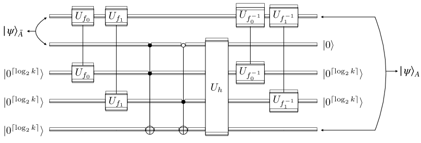
Figure 2: A quantum circuit that performs the transformation in (5). The first row denotes the $\lceil\log_{2}d\rceil$ qubits involved in encoding $x$. The second row denotes the single qubit involved in encoding $y$. The third and fourth row each denote the $\lceil\log_{2}k\rceil$ ancillary qubits designed to hold the intermediate computation of $f_{0}(x)$ and $f_{1}(x)$ respectively. The fifth row denotes the $\lceil\log_{2}k\rceil$ qubits designed to hold the output $f_{y}(x)$.

We form the augmented state $\overline{\ket{\psi}_{\bar{{\mathcal{A}}}}}$ by appending $3\lceil\log_{2}k\rceil$ qubits in the state $\ket{0}$ to the input $\ket{\psi}_{\bar{{\mathcal{A}}}}$. We intend to use one set of $\lceil\log_{2}k\rceil$ qubits to encode each of $f_{0}(x)$, $f_{1}(x)$ (both ancillary) and $f_{y}(x)$ (solution). First, we pass the qubits encoding $x$ and one set of $\lceil\log_{2}k\rceil$ qubits in the state $\ket{0}$ to the quantum oracle $U_{f_{0}}$. From this, we transform

$$\overline{\ket{\psi}_{\bar{{\mathcal{A}}}}}=\sum_{x\in[d]}\sqrt{D(x)}\ket{x,y,0^{3\lceil\log_{2}k\rceil}}\mapsto\sum_{x\in[d]}\sqrt{D(x)}\ket{x,y,f_{0}(x),0^{2\lceil\log_{2}k\rceil}}.$$

Next, we pass the qubits encoding $x$ and another set of $\lceil\log_{2}k\rceil$ qubits in the state $\ket{0}$ to the quantum oracle $U_{f_{1}}$. From this, we transform

$$\sum_{x\in[d]}\sqrt{D(x)}\ket{x,y,f_{0}(x),0^{2\lceil\log_{2}k\rceil}}\mapsto\sum_{x\in[d]}\sqrt{D(x)}\ket{x,y,f_{0}(x),f_{1}(x),0^{\lceil\log_{2}k\rceil}}.$$

Now, we apply $\lceil\log_{2}k\rceil$ TOFFOLI gates to each set of the qubit encoding $y$, a qubit involved in encoding $f_{1}(x)$ and a qubit $\ket{0}$ in the set of $\lceil\log_{2}k\rceil$ remaining qubits that have been yet been unoperated on (that are designed hold the final result $f_{y}(x)$). From this, we transform

$$\sum_{x\in[d]}\sqrt{D(x)}\ket{x,y,f_{0}(x),f_{1}(x),0^{\lceil\log_{2}k\rceil}}\mapsto\sum_{x\in[d]}\sqrt{D(x)}\ket{x,y,f_{0}(x),f_{1}(x),y.f_{1}(x)}.$$

Next, we apply the X gate to the qubit encoding $y$, and then apply $\lceil\log_{2}k\rceil$ TOFFOLI gates to each set of the qubit (now encoding) $1-y$, a qubit involved in encoding $f_{0}(x)$ and a qubit that is holding the final result. Finally, we apply the X gate again to the qubit encoding $1-y$ to revert the effect of the first X gate. All together, we have transformed

$$\sum_{x\in[d]}\sqrt{D(x)}\ket{x,y,f_{0}(x),f_{1}(x),y.f_{1}(x)} \mapsto\sum_{x\in[d]}\sqrt{D(x)}\ket{x,1-y,f_{0}(x),f_{1}(x),y.f_{1}(x)}$$

$$\mapsto\sum_{x\in[d]}\sqrt{D(x)}\ket{x,1-y,f_{0}(x),f_{1}(x),y.f_{1}(x)\oplus(1-y).f_{0}(x)}$$

$$\mapsto\sum_{x\in[d]}\sqrt{D(x)}\ket{x,y,f_{0}(x),f_{1}(x),y.f_{1}(x)\oplus(1-y).f_{0}(x)}$$

$$=\sum_{x\in[d]}\sqrt{D(x)}\ket{x,y,f_{0}(x),f_{1}(x),f_{y}(x)},$$

where, in the last line, we recognize that $y.f_{1}(x)\oplus(1-y).f_{0}(x)=f_{y}(x)$.

Now that we have computed our solution, $f_{y}(x)$, to ensure we are not introducing extraneous outputs to satisfy reversibility of unitary computation, we must uncompute all ancillary qubits to their original form. Furthermore, we also do not want the input $\ket{y}$ in our output, and would like to “remove” it, by transforming it to the $\ket{0}$ state. We proceed with the uncomputation as follows. First, we claim, with the following subproof, that there exists a (genuine) boolean function $h$ that takes as input $f_{0}(x),f_{1}(x)$, and $f_{y}(x)$ and outputs $y$.

For a short (sub)proof-by-contradiction, consider a particular input $f_{0}(x),f_{1}(x)$, and $f_{y}(x)=y.f_{1}(x)\oplus(1-y).f_{0}(x)$ (for some $x$) that maps to both $y=0$ and $y=1$. This would imply that $f_{0}(x)=f_{1}(x)$ for that particular $x$. However, as $f_{0}$ and $f_{1}$ are witnesses of the N-shattering of ${\mathcal{H}}$, they must disagree on all inputs $x$, providing us with the contradiction.

As $h$ is a genuine (boolean) function, we can apply the oracle $U_{h}$ to the qubits encoding $f_{0}(x),f_{1}(x)$, and $f_{y}(x)$ and the qubit encoding $y$. This gives us the transformation

$$\sum_{x\in[d]}\sqrt{D(x)}\ket{x,y,f_{0}(x),f_{1}(x),f_{y}(x)} \mapsto\sum_{x\in[d]}\sqrt{D(x)}\ket{x,y\oplus y,f_{0}(x),f_{1}(x),f_{y}(x)}$$

$$=\sum_{x\in[d]}\sqrt{D(x)}\ket{x,0,f_{0}(x),f_{1}(x),f_{y}(x)}.$$

Lastly, we apply $U_{f_{0}^{-1}}$ to the qubits encoding $x$ and the ancillary qubits encoding $f_{0}(x)$. And then, we apply $U_{f_{1}^{-1}}$ to the qubits encoding $x$ and the ancillary qubits encoding $f_{1}(x)$. All together, we have transformed,

$$\sum_{x\in[d]}\sqrt{D(x)}\ket{x,0,f_{0}(x),f_{1}(x),f_{y}(x)} \mapsto\sum_{x\in[d]}\sqrt{D(x)}\ket{x,0,0^{\lceil\log_{2}k\rceil},f_{1}(x),f_{y}(x)}$$

$$\mapsto\sum_{x\in[d]}\sqrt{D(x)}\ket{x,0,0^{2\lceil\log_{2}k\rceil},f_{y}(x)}=\overline{\ket{\psi}_{{\mathcal{A}}}}.$$

Now that we have performed the transformation in (5) quantumly, ignoring ancillary (and the “removed” $y$) qubits in the output, we note that the output of the transformation in (4) is attained.

The learner $\bar{{\mathcal{A}}}$ now feeds the $m$-copies of $\sum_{x\in[d]}\sqrt{D(x)}\ket{x,f_{y}(x)}$ as input to the quantum learner ${\mathcal{A}}$ and obtains (from ${\mathcal{A}}$) a classical (black box) function $g:S\to{\mathcal{Y}}$ (recall $S=\{s_{1},\ldots,s_{d}\}\subseteq{\mathcal{X}}$ is the subset that is N-shattered by ${\mathcal{H}}$). Finally, $\bar{{\mathcal{A}}}$ outputs the hypothesis (as a black box function) $f:[d]\to\{0,1\}$, given by $f(i)=1$ if and only if $g(s_{i})=f_{1}(s_{i})$ (which by construction learns ${\mathcal{H}}_{d}$).

∎

3.2.2 Upper Bounds

In general, classical sample complexity upper bounds trivially translate to the corresponding quantum ones, as the quantum learner always has the option of simply performing a measurement on each quantum example, and perform the classical learning algorithm on the resulting $m$ classical examples. We include the theorem statement (Theorem 3.8) and proof below for completeness.

Theorem 3.8 (Sample complexity upper bounds for quantum batch multiclass classification).

Let ${\mathcal{H}}\subseteq{\mathcal{Y}}^{\mathcal{X}}$, with $|{\mathcal{Y}}|=k>2$. The sample complexity of an $(\epsilon,\delta)$-quantum PAC learner (and, respectively, an $(\epsilon,\delta)$-quantum agnostic learner) for the hypothesis class ${\mathcal{H}}$ is bounded above as follows:

$$m^{\text{PAC}}=\mathcal{O}\Bigg{(}\frac{\text{Ndim}({\mathcal{H}})\log(k)\log(\frac{1}{\epsilon})+\log(\frac{1}{\delta})}{\epsilon}\Bigg{)},\;\;\text{and}\;\;\;m^{\text{agnostic}}=\mathcal{O}\Bigg{(}\frac{\text{Ndim}({\mathcal{H}})\log(k)+\log(\frac{1}{\delta})}{\epsilon^{2}}\Bigg{)}.$$

Proof.

The quantum PAC (resp. quantum agnostic) learner performs a measurement on each of the $m$ examples $\sum_{x}\sqrt{D(x)}\ket{x,y}$ (corresp. $\sum_{x,y}\sqrt{D(x,y)}\ket{x,y}$) in the standard computational basis. This provides $m$ classical examples, i.e. gives us the training set $\{(x_{i},y_{i})\}_{i=1}^{m}$, where a given $(x_{i},y_{i})$ appears with probability $D(x_{i})$ (corresp. $D(x_{i},y_{i})$). Now, the quantum PAC (resp. quantum agnostic) learners calls upon an $(\epsilon,\delta)$-PAC (resp. agnostic) classical learner to learn on the training set $\{(x_{i},y_{i})\}_{i=1}^{m}$, and outputs the resulting classically learned hypothesis. Thus, the classical sample complexity sufficiency requirements (Daniely et al., 2015; Ben-David et al., 1995) continue to hold, and our proof is complete. ∎

In Daniely et al. (2015), the classical upper bound

$$m^{\text{PAC}}=\mathcal{O}\Bigg{(}\frac{\text{Ndim}({\mathcal{H}})(\log(k)+\log(\frac{1}{\epsilon})+\log(\text{Ndim}({\mathcal{H}})))+\log(\frac{1}{\delta})}{\epsilon}\Bigg{)},$$

was shown to hold which has a tighter dependence on $\epsilon$, but a looser dependence on $\text{Ndim}({\mathcal{H}})$. The proof above naturally extends this bound too to the quantum case.

4 Classical Online Learning

So far, we have been working with learning in the batch setting, where we are provided with all the examples at once. For several practical applications, it is either impossible to obtain all the examples at once (e.g., recommendation systems), or we simply wish to evolve our learning over time. In these cases, online learning (Littlestone, 1988) – where we iteratively improve our hypothesis using examples we receive over time, and using our current hypothesis to predict for the upcoming example – is the appropriate framework to be placing ourselves in. First, we will introduce known models and results in classical online learning, and a classical generalization in Section 4.2 that, in turn, provides us with a quantum online learning model (Section 5) as a natural generalization. For ease of exposition, we begin with a treatment of boolean function classes in the realizable setting.

4.1 Adversary provides an input

Let ${\mathcal{C}}:=\{c:{\mathcal{X}}\to\{0,1\}\}$, and ${\mathcal{H}}\subseteq{\mathcal{C}}$ (i.e., ${\mathcal{H}}\subseteq\{0,1\}^{\mathcal{X}}$). A protocol for online learning is a $T$-round procedure described as follows: at the $t$-th round,

1. Adversary provides input point in the domain: $x_{t}\in{\mathcal{X}}$.

2. Learner uses a hypothesis $h_{t}\in{\mathcal{C}}$, and makes the prediction $\hat{y}_{t}=h_{t}(x_{t})\in\{0,1\}$.

3. Adversary provides the input point’s label, $y_{t}=h^{\star}(x_{t})$, where $h^{\star}\in{\mathcal{H}}$.

4. Learner suffers a loss of 1 (a ‘mistake’), if $\hat{y}_{t}\neq y_{t}$, i.e. $\mathcal{L}_{\mathbb{I}}(h_{t},x_{t},h^{\star})=\mathbf{1}[h_{t}(x_{t})\neq h^{\star}(x_{t})]$.

Therefore, the learner’s total loss is given by,

$$\mathcal{L}_{\mathbb{I}}(\mathbf{h},\mathbf{x},h^{\star})=\sum_{t=1}^{T}\mathcal{L}_{\mathbb{I}}(h_{t},x_{t},h^{\star})=\sum_{t=1}^{T}\mathbf{1}[h_{t}(x_{t})\neq h^{\star}(x_{t})],$$ (6)

where we use $\mathbf{h}:=(h_{1},\ldots,h_{T})$ to denote the sequence of hypotheses that the learner uses, and $\mathbf{x}:=(x_{1},\ldots,x_{T})$ to denote the sequence of instances that the adversary provides. The subscript $\mathbb{I}$ (in $\mathcal{L}_{\mathbb{I}}$) indicates that this is the input-based indicator (0-1) loss function.

The learner chooses an algorithm ${\mathcal{A}}$ that will generate the sequence $\mathbf{h}_{\mathcal{A}}$ following the protocol above. The learner’s goal is to minimize $\mathcal{L}_{\mathbb{I}}(\mathbf{h}_{\mathcal{A}},{\mathcal{H}})=\sup_{\mathbf{x},h^{\star}\in{\mathcal{H}}}\mathds{E}[\mathcal{L}_{\mathbb{I}}(\mathbf{h}_{\mathcal{A}},\mathbf{x},h^{\star})]$, i.e., make as few mistakes, on average, as possible regardless of the adversary’s (potentially worst-case) choices of sequence of instances $\mathbf{x}:=(x_{1},\ldots,x_{T})$ and labeling function $h^{\star}\in{\mathcal{H}}$. For the subsequent bound on $\mathcal{L}_{\mathbb{I}}(\mathbf{h}_{\mathcal{A}},{\mathcal{H}})$, we first define the combinatorial parameter, Littlestone dimension, $\text{Ldim}({\mathcal{H}})$.

Definition 4.1 (Littlestone dimension).

Let $T$ be a rooted tree whose internal nodes are labeled by elements from ${\mathcal{X}}$. Each internal node’s left edge and right edge are labeled 0 and 1, respectively. The tree $T$ is L-shattered by ${\mathcal{H}}$ if, for every path from root to leaf which traverses the nodes $x_{1},\ldots,x_{d}$, there exists a hypothesis $h\in{\mathcal{H}}$ such that, for all $i$, $h(x_{i})$ is the label of the edge $(x_{i},x_{i+1})$. We define the Littlestone dimension, $\text{Ldim}({\mathcal{H}})$, to be the maximal depth of a complete binary tree that is L-shattered by ${\mathcal{H}}$.

The classical online learning model in this subsection (Section 4.1) has been thoroughly studied, and the following theorem characterizes it in terms of the Littlestone dimension.

Theorem 4.2 (Bounds on $\mathcal{L}_{\mathbb{I}}(\mathbf{h}_{\mathcal{A}},{\mathcal{H}})$ for the canonical classical online model; Corollary 21.8 in Shalev-Shwartz and Ben-David (2014) and Theorem 24 in Daniely et al. (2015)).

Let ${\mathcal{H}}\subseteq\{0,1\}^{\mathcal{X}}$ be a hypothesis class. The Standard Optimal Algorithm (SOA) is a deterministic algorithm that achieves a worst-case total loss of $\text{Ldim}({\mathcal{H}})$, i.e. $\mathcal{L}_{\mathbb{I}}(\mathbf{h}_{SOA},{\mathcal{H}})=\text{Ldim}({\mathcal{H}})$. Furthermore, for any algorithm ${\mathcal{A}}$, the expected total loss on the worst-case sequence is at least $\frac{1}{2}\cdot\text{Ldim}({\mathcal{H}})$, i.e. $\mathcal{L}_{\mathbb{I}}(\mathbf{h}_{\mathcal{A}},{\mathcal{H}})\geq\frac{1}{2}\cdot\text{Ldim}({\mathcal{H}})$.

4.1.1 Can we obtain a quantum generalization of the classical online model?

Given the popularity and widespread applications of the classical online model, we explore the feasibility of developing a quantum version of the above online model to ultimately inquire whether such a quantum adaptation would be any more powerful from the perspective of the learner and/or the adversary. In essence, as there exists a well-defined “landscape” for classical and quantum batch learning, we seek to delineate the analogous landscape in the online learning context.

To this, if one attempts to naïvely generalize the above classical model to the quantum setting, an obvious issue arises: the quantum examples of the form (1) do not split the input-label pair. In particular, an adversary cannot temporally separate its provision of the input point and its label. A first step towards a model that can be generalized to the quantum setting, then, is to reorder the steps at the $t$-th round to $2,1\,\&\,3,4$ (i.e. where the learner provides a prediction $\hat{y_{t}}$ after which the adversary presents both the input and its label $(x_{t},y_{t})$).

While this reordering gives an entirely equivalent model that is, once again, characterized by Littlestone dimension (Theorem 4.2), it is not sufficient for a natural quantum generalization. The issue now is that a classical adversary only ever presents one (classical) example at each round. How do we go about generalizing a single classical example to a quantum adversary’s (quantum) example that, in general, sits in superposition? It appears futile to attempt to do so. The missing piece, evidently, is the lack of a notion of a distribution over examples in the classical online model(s) examined so far.

4.2 Adversary provides a distribution

Now that we have identified the unfilled gap to transition to the quantum setting, we first state the appropriate classical generalization of the canonical classical model (in Section 4.1) by asking the adversary to, at each $t$, choose a distribution over a set of input-label pairs, from which an explicit input-label pair is then drawn. The protocol for the $T$-round procedure will be as follows: at the $t$-th round,

1. Learner provides a hypothesis $h_{t}\in{\mathcal{C}}$.

2. Adversary chooses a distribution $D_{t}:{\mathcal{X}}\to[0,1]$ on the instance space, draws $x\sim D_{t}$, and reveals $(x,h^{\star}(x))$ to the learner, where $h^{\star}\in{\mathcal{H}}$.

3. Learner suffers, but does not “see”, a loss of $\mathcal{L}_{P}(h_{t},D_{t},h^{\star}):=\mathds{P}_{x\sim D_{t}}(h_{t}(x)\neq h^{\star}(x))$.

Here, the learner’s total loss is given by,

$$\mathcal{L}_{P}(\mathbf{h},\mathbf{D},h^{\star})=\sum_{t=1}^{T}\mathcal{L}_{P}(h_{t},D_{t},h^{\star})=\sum_{t=1}^{T}\mathds{P}_{x\sim D_{t}}(h_{t}(x)\neq h^{\star}(x)),$$ (7)

where we additionally use $\mathbf{D}:=(D_{1},\ldots,D_{T})$ to denote the sequence of distributions that the adversary chooses. Analogously, the learner’s objective is to choose $\mathbf{h}$ to minimize $\mathcal{L}_{P}(\mathbf{h},{\mathcal{H}})=\sup_{\mathbf{D},\,h^{\star}\in{\mathcal{H}}}\mathds{E}[\mathcal{L}_{P}(\mathbf{h},\mathbf{D},h^{\star})]$.

We identify this model as the adaptive adversary variant of the online learning model recently considered in Dawid and Tewari (2022). Note that, if we restrict the adversary, allowing it to choose only point masses, we recover the reordered model in Section 4.1.

From a learning standpoint, the adversary-provides-a-distribution model differs fundamentally from the canonical model in that the learner, here, does not have full information about its own loss at any given round. Since the learner does not know $D_{t}$, it cannot compute $\mathcal{L}_{P}(h_{t},D_{t},h^{\star})$ for any $t$. In other words, the learner seeks to minimize a quantity that it cannot even compute. This partial information setting here, at least at first, appears to be more challenging for the learner as it not only grapples with the inability to compute its loss but also contends with the larger space available to the adversary for its choices ($D_{t}\in[0,1]^{\mathcal{X}}$ vs. $x_{t}\in\{0,1\}^{\mathcal{X}}$).

However, as we will soon illustrate, this perceived challenge proves not to be the case. The key factor influencing this distinction lies in the learner’s ability to calculate $\mathcal{L}_{\mathbb{I}}(\mathbf{h},\mathbf{x},h^{\star})$ for the observed sequence of examples $\mathbf{x}$, providing an unbiased estimator for its total loss $\mathcal{L}_{P}(\mathbf{h},\mathbf{D},h^{\star})$. We demonstrate that it is indeed (necessary and) sufficient for a learner in the adversary-provides-a-distribution model to execute SOA on the observed sequence of examples $\mathbf{x}$ to achieve a bound analogous to that in the canonical model (cf. Theorem 4.2). Before delving into the results, we formally define what a learner, an adversary, and learnability entails for the adversary-provides-a-distribution model we have just discussed.

Definition 4.3 (Classical online learner).

An algorithm ${\mathcal{A}}$ is a classical online learner for a hypothesis class ${\mathcal{H}}\subseteq{\mathcal{C}}$ if having received a sequence of examples over the first $t$ rounds,
$(x_{1},h^{\star}(x_{1})),\ldots,(x_{t},h^{\star}(x_{t}))$ where $x_{i}\sim D_{i}$ with $D_{i}$ arbitrary (unknown), ${\mathcal{A}}$ outputs a hypothesis $h_{t+1}\in{\mathcal{C}}$ at round $t+1$.

Definition 4.4 (Classical adversary).

Having received a sequence of hypothesis $\mathbf{h}|_{t}=(h_{1},\ldots,h_{t})$ from the learner, and a sequence of examples $\mathbf{x}|_{t}=(x_{t},\ldots,x_{t})$ drawn previously from its own prior choices of distributions $\mathbf{D}|_{t}=(D_{1},\ldots,D_{t})$ over the first $t$ rounds, at round $t+1$, a classical (online) adversary chooses a distribution $D_{t+1}:{\mathcal{X}}\to[0,1]$ on the instance space, draws $x_{t+1}\in D_{t+1}$ and reveals $(x_{t+1},h^{\star}(x_{t+1}))$ to the learner, where $h^{\star}\in{\mathcal{H}}$ is consistent with all preceding labeled examples.

Definition 4.5 (Classical online learnability).

A hypothesis class ${\mathcal{H}}$ is classical online learnable if there exists a classical online learning algorithm ${\mathcal{A}}$ such that $\mathcal{L}_{P}(\mathbf{h}_{\mathcal{A}},{\mathcal{H}})=\sup_{\mathbf{D},\,h^{\star}\in{\mathcal{H}}}\mathds{E}[\mathcal{L}_{P}(\mathbf{h}_{\mathcal{A}},\mathbf{D},h^{\star})]=o(T)$.

With these definitions in place, our next objective is to characterize learnability in the adversary-provides-a-distribution framework. When we later introduce the quantum online learning model (Section 5), these classical insights will serve as a foundation, enabling us to draw direct comparisons and understand the strong links connecting the classical adversary-provides-a-distribution model to the quantum online learning setup.

Theorem 4.6 (Upper bound on the expected loss for the classical adversary-provides-a-distribution model).

Let ${\mathcal{H}}\subseteq\{0,1\}^{\mathcal{X}}$ be a hypothesis class, and $h^{\star}\in{\mathcal{H}}$. For every adversary, there exists a classical online learner for ${\mathcal{H}}$ that satisfies

$$\mathds{E}[\mathcal{L}_{P}(\mathbf{h},\mathbf{D},h^{\star})]=\mathcal{O}(\text{Ldim}({\mathcal{H}})).$$

Proof.

Let $\mathbf{D}$ and $h^{\star}\in{\mathcal{H}}$ be arbitrarily chosen. We proceed by first obtaining a high-probability bound for $\mathcal{L}_{P}(\mathbf{h},\mathbf{D},h^{\star})$, and then converting it to an in-expectation one. To obtain the high-probability bound, we begin by establishing that the difference between $\mathcal{L}_{P}(\mathbf{h},\mathbf{D},h^{\star})$ and $\mathcal{L}_{\mathbb{I}}(\mathbf{h},\mathbf{x},h^{\star})$ (see Section 4.1, (6)) on the revealed stream of examples $\mathbf{x}=(x_{t})_{t=1}^{T}$ (with each $x_{t}\sim D_{t}$) is the sum of a martingale difference sequence.

Let $M_{t}:=\underbrace{\mathcal{L}_{P}(h_{t},D_{t},h^{\star})}_{P_{t}}-\underbrace{\mathcal{L}_{\mathbb{I}}(h_{t},x_{t},h^{\star})}_{I_{t}}$, where $x_{t}\sim D_{t}$. With the filtration $\mathbb{F}:=(\mathcal{F}_{t})_{t=1}^{T}$, where $\mathcal{F}_{t}$ corresponds to the information revealed up to (and, including) round $t$, namely $\mathbf{h}|_{t}$, $\mathbf{D}|_{t}$ and $\mathbf{x}|_{t}$, we note that $\mathbf{M}:=(M_{t})_{t=1}^{T}$ is adapted to $\mathbb{F}$ and $\forall t$,

$$\mathds{E}[M_{t}] =\mathds{E}[P_{t}]-\mathds{E}[I_{t}]<\infty$$

$$\mathds{E}[M_{t}|\mathcal{F}_{t-1}] =\mathds{E}[P_{t}|\mathcal{F}_{t-1}]-\mathds{E}[I_{t}|\mathcal{F}_{t-1}]=P_{t}-P_{t}=0,$$

where the first line is due to the boundedness ($0\leq P_{t},I_{t}\leq 1,\;\forall t$) of $P_{t}$ and $I_{t}$. And, the second line is due to $\mathds{E}[I_{t}|\mathcal{F}_{t-1}]=1\cdot\mathds{P}_{x_{t}\sim D_{t}}(h_{t}(x_{t})\neq h^{\star}(x_{t}))+0\cdot\mathds{P}_{x_{t}\sim D_{t}}(h_{t}(x_{t})=h^{\star}(x_{t}))=P_{t}$. Therefore, $\mathbf{M}$ is a martingale difference sequence. Now, for any $t$,

$$M_{t}^{2}=(P_{t}-I_{t})^{2} \leq P_{t}^{2}+I_{t}^{2}$$

$$\leq P_{t}+I_{t},$$

where both the first and second lines are due to $0\leq P_{t},I_{t}\leq 1,\;\forall t$. Therefore, we can bound the predictable quadratic variation $\langle M_{T}\rangle$ of $\mathbf{M}$, as follows:

$$\langle M_{T}\rangle:=\sum_{t=1}^{T}\mathds{E}[M_{t}^{2}|\mathcal{F}_{t-1}]\leq\sum_{t=1}^{T}(P_{t}+I_{t})=\sum_{t=1}^{T}P_{t}+\sum_{t=1}^{T}I_{t}\leq\sum_{t=1}^{T}P_{t}+\text{Ldim}({\mathcal{H}}),$$ (8)

where the final inequality is due to the classical online bound (via SOA) on $\sum_{t=1}^{T}I_{t}$ (Theorem 4.2). Now, by Theorem 1 of Beygelzimer et al. (2011), with probability $1-\delta$ (for any $\delta>0$), we have

$$\sum_{t=1}^{T}M_{t} \leq\log\Big{(}\frac{1}{\delta}\Big{)}+(e-2)\langle M_{T}\rangle\iff\sum_{t=1}^{T}P_{t}\leq\sum_{t=1}^{T}I_{t}+\log\Big{(}\frac{1}{\delta}\Big{)}+(e-2)\langle M_{T}\rangle.$$

Note here that $\sum_{t=1}^{T}P_{t}=\mathcal{L}_{P}(\mathbf{h},\mathbf{D},h^{\star})$. Therefore, appealing again to Theorem 4.2 and the inequality on $\langle M_{T}\rangle$ in (8), we have that (with probability $1-\delta$),

$$\mathcal{L}_{P}(\mathbf{h},\mathbf{D},h^{\star}) \leq\text{Ldim}({\mathcal{H}})+\log\Big{(}\frac{1}{\delta}\Big{)}+(e-2)(\mathcal{L}_{P}(\mathbf{h},\mathbf{D},h^{\star})+\text{Ldim}({\mathcal{H}}))$$

$$\implies\mathcal{L}_{P}(\mathbf{h},\mathbf{D},h^{\star}) \leq\frac{1+(e-2)}{1-(e-2)}\text{Ldim}({\mathcal{H}})+\frac{1}{1-(e-2)}\log\Big{(}\frac{1}{\delta}\Big{)}$$

$$\leq 7\cdot\text{Ldim}({\mathcal{H}})+\frac{1}{3}\log\Big{(}\frac{1}{\delta}\Big{)}.$$

or equivalently, for any $\delta>0$,

$$\mathds{P}\Big{[}\mathcal{L}_{P}(\mathbf{h},\mathbf{D},h^{\star})>7\cdot\text{Ldim}({\mathcal{H}})+\frac{\delta}{3}\Big{]}\leq e^{-\delta}.$$ (9)

Now, we compute the in-expectation bound (i.e. a bound on $\mathds{E}[\mathcal{L}_{P}(\mathbf{h},\mathbf{D},h^{\star})]$) guaranteed by the above tail bound (9).

$$\mathds{E}[\mathcal{L}_{P}(\mathbf{h},\mathbf{D},h^{\star})] =\int_{0}^{\infty}\mathds{P}[\mathcal{L}_{P}(\mathbf{h},\mathbf{D},h^{\star})>\ell]\,d\ell$$

$$=\int_{0}^{7\cdot\text{Ldim}({\mathcal{H}})}\mathds{P}[\mathcal{L}_{P}(\mathbf{h},\mathbf{D},h^{\star})>\ell]\,d\ell+\int_{7\cdot\text{Ldim}({\mathcal{H}})}^{\infty}\mathds{P}[\mathcal{L}_{P}(\mathbf{h},\mathbf{D},h^{\star})>\ell]\,d\ell$$

$$=\int_{0}^{7\cdot\text{Ldim}({\mathcal{H}})}\mathds{P}[\mathcal{L}_{P}(\mathbf{h},\mathbf{D},h^{\star})>\ell]\,d\ell+\frac{1}{3}\int_{0}^{\infty}\mathds{P}\Big{[}\mathcal{L}_{P}(\mathbf{h},\mathbf{D},h^{\star})>7\cdot\text{Ldim}({\mathcal{H}})+\frac{\delta}{3}\Big{]}\,d\delta$$

$$\leq\int_{0}^{7\cdot\text{Ldim}({\mathcal{H}})}1\,d\ell+\frac{1}{3}\int_{0}^{\infty}e^{-\delta}\,d\delta$$

$$=7\cdot\text{Ldim}({\mathcal{H}})+\frac{1}{3}$$

$$=\mathcal{O}(\text{Ldim}({\mathcal{H}})),$$

where the first line holds as $\mathcal{L}_{P}(\mathbf{h},\mathbf{D},h^{\star})\geq 0$, the third line uses the change of variable $\ell=7\cdot\text{Ldim}({\mathcal{H}})+\frac{\delta}{3}$, the fourth line uses a naïve bound of $\mathds{P}[\mathcal{L}_{P}(\mathbf{h},\mathbf{D},h^{\star})>\ell]\leq 1$ (for $0\leq\ell\leq 7\cdot\text{Ldim}({\mathcal{H}})$) on the first integral, and our high-probability bound in (9) on the second integral. ∎

To summarize, Theorem 4.6 tells us that $\text{Ldim}({\mathcal{H}})$ continues to be a sufficient condition for learnability under the new (adversary-provides-a-distribution) model in Section 4.2. In other words, a learner that performs SOA on the observed sequence of examples $\mathbf{x}$ only suffers a constant overhead under the adversary-provides-a-distribution model as compared to SOA under the canonical online model (Section 4.1). Next, we show (Theorem 4.7) that $\text{Ldim}({\mathcal{H}})$ is also a necessary condition for learnability, and thus fully characterizes the learnability of the adversary-provides-a-distribution model.

Theorem 4.7 (Lower bound on the expected loss for the classical adversary-provides-a-distribution model).

Let ${\mathcal{H}}\subseteq\{0,1\}^{\mathcal{X}}$ be a hypothesis class, and $h^{\star}\in{\mathcal{H}}$. For every classical online learner of ${\mathcal{H}}$, there exists an adversary such that

$$\mathds{E}[\mathcal{L}_{P}(\mathbf{h},\mathbf{D},h^{\star})]=\Omega(\text{Ldim}({\mathcal{H}})).$$

Proof.

Consider an adversary which chooses each $D_{t}$ to be a point mass on the instance space, i.e. the adversary simply chooses an instance $x_{t}$ at each $t$. Since each $x_{t}\sim D_{t}$ is deterministic, we have

$$\mathcal{L}_{P}(\mathbf{h},\mathbf{D},h^{\star})=\mathcal{L}_{\mathbb{I}}(\mathbf{h},\mathbf{x},h^{\star})=\Omega(\text{Ldim}({\mathcal{H}})),$$

where the second equality is due to (the lower bound part of) Theorem 4.2. By taking expectations, we conclude our proof. ∎

Now that we have characterized the learnability of the adversary-provides-a-distribution model in Section 4.2 (via Theorems 4.6 and 4.7), we proceed to introduce and present results for related classical online models which arise from successively relaxing, first, the realizability assumption and then, the boolean function class assumption. These serve to define our scope and lay the groundwork for a comprehensive understanding before introducing the anticipated quantum generalization.

4.3 Adversary provides a distribution in the agnostic setting

In the agnostic framework, we dispense with the realizability assumption that $h^{\star}\in{\mathcal{H}}$ (i.e., the labels need not be consistent with any hypothesis in the hypothesis class). In fact, the labels need not arise from a labeling function at all, i.e., the examples may be inconsistent. The agnostic generalization of the adversary-provides-a-distribution model in Section 4.2 is given by the following protocol for the $T$-round procedure: at the $t$-th round,

1. Learner provides a hypothesis $h_{t}\in{\mathcal{C}}$.

2. Adversary chooses a distribution $D_{t}:\{0,1\}^{n+1}\to[0,1]$ on the instance space, draws and reveals $z_{t}=(x_{t},y_{t})\sim D_{t}$ to the learner.

3. Learner suffers, but does not “see”, a loss of $\mathcal{L}_{P}(h_{t},D_{t}):=\mathds{P}_{(x,y)\sim D_{t}}(h_{t}(x)\neq y)$.

As there may be no hypothesis that provides the true label on every instance over the $T$ rounds, we resort to comparing the learner to the best fixed hypothesis in ${\mathcal{H}}$ in hindsight. In other words, the learner’s total regret is given by,

$$\mathcal{R}_{P}(\mathbf{h},\mathbf{D},{\mathcal{H}})=\sum_{t=1}^{T}{\mathcal{L}}_{P}(h_{t},D_{t})-\inf_{h\in{\mathcal{H}}}\sum_{t=1}^{T}{\mathcal{L}}_{P}(h,D_{t}).$$ (10)

Definitions 4.3, 4.4, and 4.5 are adapted analogously to give us the notions of a classical online learner, adversary and learnability in the agnostic setting. Additionally, we introduce further notation and definitions to facilitate the subsequent theorem.

An ${\mathcal{X}}$-valued tree $\underline{X}$ of depth $T$ is a rooted complete binary tree with nodes labeled by elements of ${\mathcal{X}}$. We identify the tree $\underline{X}$ with the sequence $x^{(1)},\ldots,x^{(T)}$ of labeling functions $x^{(i)}:\{\pm 1\}^{i-1}\to{\mathcal{X}}$ which provide the labels for each node. Here, $x^{(1)}$ labels the root of the tree, and $x^{(i)}$ for $i>1$ labels the node obtained by following the path of length $i-1$ from the root, with $+1$ indicating ‘right’ and $-1$ indicating ‘left’. A path of length $T$ is given by the sequence $\epsilon=(\epsilon_{1},\ldots,\epsilon_{T})\in\{\pm 1\}^{T}$. We denote the label at round $t$ along this path as $x^{(t)}(\epsilon)$, understanding that $x^{(t)}$ depends only on the prefix $(\epsilon_{1},\ldots,\epsilon_{t-1})$ of $\epsilon$. With this notion of a tree, we define the sequential Rademacher complexity of a hypothesis class, ${\mathcal{H}}\subseteq{\mathcal{Y}}^{\mathcal{X}}$ (Rakhlin et al., 2015).

Definition 4.8 (Sequential Rademacher complexity of ${\mathcal{H}}$).

The sequential Rademacher complexity of a function class ${\mathcal{H}}\subseteq{\mathcal{Y}}^{\mathcal{X}}$ on an ${\mathcal{X}}$-valued tree $\underline{X}$ is defined as

$$\mathfrak{R}_{T}({\mathcal{H}},\underline{X})=\mathds{E}\Big{[}\sup_{h\in{\mathcal{H}}}\frac{1}{T}\sum_{t=1}^{T}\epsilon_{t}h(x^{(t)}(\mathbf{\epsilon}))\Big{]},$$

and

$$\mathfrak{R}_{T}({\mathcal{H}})=\sup_{\underline{X}}\mathfrak{R}_{T}({\mathcal{H}},\underline{X}),$$

where the outer supremum is taken over all ${\mathcal{X}}$-valued trees of depth $T$; $\mathbf{\epsilon}=(\epsilon_{1},\ldots,\epsilon_{T})\in\{\pm 1\}^{T}$ is a sequence of i.i.d. Rademacher random variables.

Definition 4.9 (The loss class $\mathcal{L}_{\mathbb{I}}\circ{\mathcal{H}}$).

The loss class, $\mathcal{L}_{\mathbb{I}}\circ{\mathcal{H}}$, is a boolean hypothesis class given by

$$\mathcal{L}_{\mathbb{I}}\circ{\mathcal{H}}=\{\mathbf{1}[h(x)\neq y]:h\in{\mathcal{H}},x\in{\mathcal{X}},y\in{\mathcal{Y}}\}.$$

Note that $\mathcal{L}_{\mathbb{I}}\circ{\mathcal{H}}\subseteq\{0,1\}^{{\mathcal{X}}\times{\mathcal{Y}}}$, and that its sequential Rademacher complexity is defined analogously to Definition 4.8. With these definitions in place, we can proceed to present the theorems for the bounds on expected regret for the adversary-provides-a-distribution model in the agnostic setting.

Theorem 4.10 (Upper bound on the expected regret for the classical adversary-provides-a-distribution model in the agnostic setting).

Let ${\mathcal{H}}\subseteq\{0,1\}^{\mathcal{X}}$ be a hypothesis class. For every adversary, there exists a classical online learner for ${\mathcal{H}}$ that satisfies

$$\mathds{E}[\mathcal{R}_{P}(\mathbf{h},\mathbf{D},{\mathcal{H}})]=\mathcal{O}(\sqrt{\text{Ldim}({\mathcal{H}})\cdot T}).$$

Proof.

Let $\mathbf{D}$ be an arbitrary sequence of distributions, and let $\mathbf{z}=(z_{1},\ldots,z_{t})$ be a sequence of instances such that $z_{i}\sim D_{i}$. Then, defining $\mathcal{R}_{\mathbb{I}}(\mathbf{h},\mathbf{z},{\mathcal{H}}):=\sum_{t=1}^{T}\mathcal{L}_{\mathbb{I}}(h_{t},z_{t})-\inf_{h\in{\mathcal{H}}}\sum_{t=1}^{T}\mathcal{L}_{\mathbb{I}}(h,z_{t})$, we have

$$\mathcal{R}_{P}(\mathbf{h},\mathbf{D},{\mathcal{H}}) =\mathcal{R}_{P}(\mathbf{h},\mathbf{D},{\mathcal{H}})-\mathcal{R}_{\mathbb{I}}(\mathbf{h},\mathbf{z},{\mathcal{H}})+\mathcal{R}_{\mathbb{I}}(\mathbf{h},\mathbf{z},{\mathcal{H}})$$

$$=\underbrace{\sum_{t=1}^{T}{\mathcal{L}}_{P}(h_{t},D_{t})-\sum_{t=1}^{T}{\mathcal{L}}_{\mathbb{I}}(h_{t},z_{t})}_{\Delta_{1}}+\underbrace{\inf_{h\in{\mathcal{H}}}\sum_{t=1}^{T}{\mathcal{L}}_{\mathbb{I}}(h,z_{t})-\inf_{h\in{\mathcal{H}}}\sum_{t=1}^{T}{\mathcal{L}}_{P}(h,D_{t})}_{\Delta_{2}}+\mathcal{R}_{\mathbb{I}}(\mathbf{h},\mathbf{z},{\mathcal{H}}).$$

We proceed by bounding the expected value of $\Delta_{1}$, $\Delta_{2}$ and $\mathcal{R}_{\mathbb{I}}(\mathbf{h},\mathbf{z},{\mathcal{H}})$ separately.

Working with $\Delta_{1}$, we let $M_{t}:={\mathcal{L}}_{P}(h_{t},D_{t})-{\mathcal{L}}_{\mathbb{I}}(h_{t},z_{t})$. With the filtration $\mathbb{F}:=(\mathcal{F}_{t})_{t=1}^{T}$, where $\mathcal{F}_{t}$ corresponds to the information revealed up to (and, including) round $t$, namely $\mathbf{h}|_{t}$, $\mathbf{D}|_{t}$ and $\mathbf{z}|_{t}$, we note that $\mathbf{M}:=(M_{t})_{t=1}^{T}$ is adapted to $\mathbb{F}$ and $\forall t$,

$$\mathds{E}[M_{t}] =\mathds{E}[{\mathcal{L}}_{P}(h_{t},D_{t})]-\mathds{E}[{\mathcal{L}}_{\mathbb{I}}(h_{t},z_{t})]<\infty$$

$$\mathds{E}[M_{t}|\mathcal{F}_{t-1}] =\mathds{E}[{\mathcal{L}}_{P}(h_{t},D_{t})|\mathcal{F}_{t-1}]-\mathds{E}[{\mathcal{L}}_{\mathbb{I}}(h_{t},z_{t})|\mathcal{F}_{t-1}]={\mathcal{L}}_{P}(h_{t},D_{t})-{\mathcal{L}}_{P}(h_{t},D_{t})=0,$$

where the first line is due to the boundedness ($0\leq{\mathcal{L}}_{P}(h_{t},D_{t}),{\mathcal{L}}_{\mathbb{I}}(h_{t},z_{t})\leq 1,\;\forall t$) of ${\mathcal{L}}_{P}(h_{t},D_{t})$ and ${\mathcal{L}}_{\mathbb{I}}(h_{t},z_{t})$. And, the second line is due to $\mathds{E}[{\mathcal{L}}_{\mathbb{I}}(h_{t},z_{t})|\mathcal{F}_{t-1}]=1\cdot\mathds{P}_{z_{t}\sim D_{t}}(h_{t}(x_{t})\neq y_{t})+0\cdot\mathds{P}_{z_{t}\sim D_{t}}(h_{t}(x_{t})=y_{t})={\mathcal{L}}_{P}(h_{t},D_{t})$. Therefore, $\mathbf{M}$ is a martingale difference sequence. Now, as $\Delta_{1}=\sum_{t=1}^{T}M_{t}$, by Azuma-Hoeffding’s inequality, since $|M_{t}|<1$ for all $t$, we have that

$$\mathds{P}[|\Delta_{1}|\geq\delta]\leq 2\exp\Big{(}-\frac{\delta^{2}}{2T}\Big{)},\;\;\text{for all}\;\;\delta\in{\mbox{{R}}}^{+},T\in\mathbb{Z}^{+}.$$ (11)

This allows us to compute the following bound on $\mathds{E}[\Delta_{1}]$:

$$\mathds{E}[\Delta_{1}]\leq\mathds{E}[|\Delta_{1}|] \leq\int_{0}^{\infty}\mathds{P}[|\Delta_{1}|\geq\delta]\,dB$$

$$\leq\int_{0}^{\infty}2\exp\Big{(}-\frac{\delta^{2}}{2T}\Big{)}\,dB=\sqrt{2\pi T}=\mathcal{O}(\sqrt{T}),$$

where the first line holds as $\Delta_{1}<|\Delta_{1}|$ (for the first inequality) and $|\Delta_{1}|\geq 0$ (for the second inequality), and the second line uses the bound in (11).

Next, working with $\Delta_{2}$, we obtain the following chain of (in)equalities:

$$\Delta_{2} =\inf_{h\in{\mathcal{H}}}\sum_{t=1}^{T}{\mathcal{L}}_{\mathbb{I}}(h,z_{t})-\inf_{h\in{\mathcal{H}}}\sum_{t=1}^{T}{\mathcal{L}}_{P}(h,D_{t})$$

$$=-\sup_{h\in{\mathcal{H}}}\sum_{t=1}^{T}-{\mathcal{L}}_{\mathbb{I}}(h,z_{t})+\sup_{h\in{\mathcal{H}}}\sum_{t=1}^{T}-{\mathcal{L}}_{P}(h,D_{t})$$

$$=-\sup_{h\in{\mathcal{H}}}\sum_{t=1}^{T}(-{\mathcal{L}}_{\mathbb{I}}(h,z_{t})+{\mathcal{L}}_{P}(h,D_{t})-{\mathcal{L}}_{P}(h,D_{t}))+\sup_{h\in{\mathcal{H}}}\sum_{t=1}^{T}-{\mathcal{L}}_{P}(h,D_{t})$$

$$\leq\sup_{h\in{\mathcal{H}}}\sum_{t=1}^{T}({\mathcal{L}}_{\mathbb{I}}(h,z_{t})-{\mathcal{L}}_{P}(h,D_{t})),$$

where the final inequality is a result of the subadditivity of the supremum; to elaborate, we derive $\sup_{h}f\leq\sup_{h}(f-g)+\sup_{h}g\iff\sup_{h}f-\sup_{h}g\leq\sup_{h}(f-g)$, to which we substitute $f=-{\mathcal{L}}_{P}(h,D_{t})$ and $g=-{\mathcal{L}}_{\mathbb{I}}(h,z_{t})+{\mathcal{L}}_{P}(h,D_{t})-{\mathcal{L}}_{P}(h,D_{t})$. So far, taking expectations both sides, we have $\mathds{E}[\Delta_{2}]\leq\mathds{E}[\sup_{h\in{\mathcal{H}}}\sum_{t=1}^{T}({\mathcal{L}}_{\mathbb{I}}(h,z_{t})-{\mathcal{L}}_{P}(h,D_{t}))]$. Next, we bound the in-expectation quantity on the right-hand side to obtain,

$$\mathds{E}\Big{[}\sup_{h\in{\mathcal{H}}}\sum_{t=1}^{T}({\mathcal{L}}_{\mathbb{I}}(h,z_{t})-{\mathcal{L}}_{P}(h,D_{t}))\Big{]} =\mathds{E}\Bigg{[}\sup_{h\in{\mathcal{H}}}\sum_{t=1}^{T}\Big{(}\mathbf{1}[h(x_{t})\neq y_{t}]-\mathds{P}_{(x_{t},y_{t})\sim D_{t}}[h(x_{t})\neq y_{t}]\Big{)}\Bigg{]}$$

$$=\mathds{E}\Bigg{[}\sup_{h\in{\mathcal{H}}}\sum_{t=1}^{T}\Big{(}\mathbf{1}[h(x_{t})\neq y_{t}]-\mathds{E}_{(x_{t},y_{t})\sim D_{t}}\Big{[}\mathbf{1}[h(x_{t})\neq y_{t}]|z_{1:t-1}\Big{]}\Big{)}\Bigg{]}$$

$$\leq 2T\cdot\mathfrak{R}_{T}(\mathcal{L}_{\mathbb{I}}\circ{\mathcal{H}})$$

$$\leq 2T\cdot\mathfrak{R}_{T}({\mathcal{H}})$$

$$=\mathcal{O}(\sqrt{\text{Ldim}({\mathcal{H}})\cdot T}),$$

where the third line is due to Theorem 2 in Rakhlin et al. (2015), the fourth line is due to Theorem 16 of Dawid and Tewari (2022) (with ${\mathcal{Y}}=\{0,1\}$) and the last line is from the proof of Theorem 12.1 in Alon et al. (2021).

Finally, also from Theorem 12.1 of Alon et al. (2021), we have $\mathcal{R}_{\mathbb{I}}(\mathbf{h},\mathbf{z},{\mathcal{H}})=\mathcal{O}(\sqrt{\text{Ldim}({\mathcal{H}})\cdot T})$. Putting everything together, using the linearity of expectation, we have,

$$\mathds{E}[\mathcal{R}_{P}(\mathbf{h},\mathbf{D},{\mathcal{H}})] =\mathds{E}[\Delta_{1}+\Delta_{2}+\mathcal{R}_{\mathbb{I}}(\mathbf{h},\mathbf{z},{\mathcal{H}})]$$

$$=\mathds{E}[\Delta_{1}]+\mathds{E}[\Delta_{2}]+\mathds{E}[\mathcal{R}_{\mathbb{I}}(\mathbf{h},\mathbf{z},{\mathcal{H}})]$$

$$=\mathcal{O}(\sqrt{T})+\mathcal{O}(\sqrt{\text{Ldim}({\mathcal{H}})\cdot T})+\mathcal{O}(\sqrt{\text{Ldim}({\mathcal{H}})\cdot T})$$

$$=\mathcal{O}(\sqrt{\text{Ldim}({\mathcal{H}})\cdot T}).$$

∎

In summary, our theorem reveals that the optimal classical learner for the canonical (adversary-provides-an-input) agnostic model, when provided with the observed sequence of instances $\mathbf{z}$ in the new protocol, experiences, at most, a constant overhead when assessed under the new (adversary-provides-a-distribution) framework. Upon closer examination, it was critical for the bound on $\mathds{E}[\Delta_{2}]$ in our proof not to be worse than the bound on $\mathds{E}[\mathcal{R}_{\mathbb{I}}(\mathbf{h},\mathbf{z},{\mathcal{H}})]$. It is noteworthy that the bound on $\mathds{E}[\Delta_{2}]$ is guaranteed by the rate of online uniform convergence (in the frameworks of the sequential Rademacher complexity (Rakhlin et al., 2015) and the adversarial (uniform) laws of large numbers (Alon et al., 2021)), whereas the bound on $\mathds{E}[\mathcal{R}_{\mathbb{I}}(\mathbf{h},\mathbf{z},{\mathcal{H}})]$ is guaranteed by the rate of canonical (agnostic) online learnability. The equivalence between these two rates, for the boolean function class case, played a pivotal role in establishing our result.

Next, we establish (Theorem 4.11) a matching lower bound for expected regret within the agnostic adversary-provides-a-distribution framework. This fully characterizes agnostic learnability under the adversary-provides-a-distribution framework. As with all lower bound proofs within this framework, we efficiently conclude the proof statement by considering an adversary that exclusively plays point masses.

Theorem 4.11 (Lower bound on the expected regret for the classical adversary-provides-a-distribution model in the agnostic setting).

Let ${\mathcal{H}}\subseteq\{0,1\}^{\mathcal{X}}$ be a hypothesis class. For every classical online learner of ${\mathcal{H}}$, there exists an adversary such that

$$\mathds{E}[\mathcal{R}_{P}(\mathbf{h},\mathbf{D},{\mathcal{H}})]=\Omega(\sqrt{\text{Ldim}({\mathcal{H}})\cdot T}).$$

Proof.

As in Theorem 4.7, we again consider an adversary which chooses each $D_{t}$ to be a point mass on the instance space, i.e. the adversary simply chooses an instance $z_{t}$ at each $t$. Since each $z_{t}\sim D_{t}$ is deterministic, we have

$$\mathds{E}[\mathcal{R}_{P}(\mathbf{h},\mathbf{D},{\mathcal{H}})]=\mathds{E}[\mathcal{R}_{\mathbb{I}}(\mathbf{h},\mathbf{z},{\mathcal{H}})]=\Omega(\sqrt{\text{Ldim}({\mathcal{H}})\cdot T}),$$

where the second equality is due to (the lower bound part of) Theorem 21.10 in Shalev-Shwartz and Ben-David (2014). ∎

4.4 Adversary provides a distribution in the multiclass setting

In Sections 4.1, 4.2 and 4.3, we considered boolean hypothesis classes, i.e. ${\mathcal{H}}\subseteq\{0,1\}^{\mathcal{X}}$. Here, we consider the adversary-provides-a-distribution models in Sections 4.2 and 4.3 extended to the setting of multiclass learning, i.e. ${\mathcal{H}}\subseteq{\mathcal{C}}:=\{c:{\mathcal{X}}\to{\mathcal{Y}}\}$, with $|{\mathcal{Y}}|>2$. As stated earlier, the objective here is to lay the groundwork, with a clear understanding of these models in the classical paradigm, before delving into their quantum generalizations.

4.4.1 Realizable setting

The online learning protocol in the realizable setting is identical to that specified in Section 4.2, with the added specification of a multiclass hypothesis (and, concept) class. To express our results in this setting, we first define the combinatorial parameter, multiclass Littlestone dimension ($\text{mcLdim}({\mathcal{H}})$), which is a generalization of the Littlestone dimension to the multiclass setting.

Definition 4.12 (Multiclass Littlestone dimension).

Let $T$ be a rooted tree whose internal nodes are labeled by elements from ${\mathcal{X}}$ and whose edges are labeled by elements from ${\mathcal{Y}}$, such that the edges from a single parent to its child nodes are each labeled with a different label. The tree $T$ is mcL-shattered by ${\mathcal{H}}$ if, for every path from root to leaf which traverses the nodes $x_{1},\ldots,x_{d}$, there exists a hypothesis $h\in{\mathcal{H}}$ such that, for all $i$, $h(x_{i})$ is the label of the edge $(x_{i},x_{i+1})$. We define the multiclass Littlestone dimension, $\text{mcLdim}({\mathcal{H}})$, to be the maximal depth of a complete binary tree that is mcL-shattered by ${\mathcal{H}}$.

Theorem 4.13 (Upper bound on the expected loss for the classical adversary-provides-a-distribution model in the multiclass setting).

Let ${\mathcal{H}}\subseteq{\mathcal{Y}}^{\mathcal{X}},\,\text{with}\;|{\mathcal{Y}}|=k>2$, be a hypothesis class, and $h^{\star}\in{\mathcal{H}}$. For every adversary, there exists a classical online learner for ${\mathcal{H}}$ that satisfies

$$\mathds{E}[\mathcal{L}_{P}(\mathbf{h},\mathbf{D},h^{\star})]=\mathcal{O}(\text{mcLdim}({\mathcal{H}})).$$

Proof.

We follow the steps in the proof of Theorem 4.6, which continue to hold in the multiclass setting, with a minor difference (upper bound on $\sum_{t=1}^{T}\mathcal{L}_{\mathbb{I}}(h_{t},x_{t},h^{\star})$ is now $\text{mcLdim}({\mathcal{H}})$, instead of $\text{Ldim}({\mathcal{H}})$) that enables us to conclude the current proof. First, we recall the preliminaries. Let $\mathbf{D}$, $h^{\star}\in{\mathcal{H}}$ be arbitrarily chosen, and define $\mathbf{M}:=(M_{t})_{t=1}^{T}$ where $M_{t}:=\underbrace{\mathcal{L}_{P}(h_{t},D_{t},h^{\star})}_{P_{t}}-\underbrace{\mathcal{L}_{\mathbb{I}}(h_{t},x_{t},h^{\star})}_{I_{t}}$, with $x_{t}\sim D_{t}$. We have shown in the proof of Theorem 4.6 that $\mathbf{M}$ is a martingale difference sequence, and that its predictable quadratic variation $\langle M_{T}\rangle$ is bounded as $\langle M_{T}\rangle\leq\sum_{t=1}^{T}P_{t}+\sum_{t=1}^{T}I_{t}$. Now, the classical upper bound in the multiclass setting on $\sum_{t=1}^{T}I_{t}$ is $\text{mcLdim}({\mathcal{H}})$ (Daniely et al. (2015), Theorem 24), giving us $\langle M_{T}\rangle\leq\sum_{t=1}^{T}P_{t}+\text{mcLdim}({\mathcal{H}})$. Applying Theorem 1 of Beygelzimer et al. (2011) and simplifying as before, we obtain, with probability $1-\delta$ (for any $\delta>0$), that

$$\mathcal{L}_{P}(\mathbf{h},\mathbf{D},h^{\star})\leq 7\cdot\text{mcLdim}({\mathcal{H}})+\frac{1}{3}\log\Big{(}\frac{1}{\delta}\Big{)},$$

which gives us the tail bound, $\mathds{P}\Big{[}\mathcal{L}_{P}(\mathbf{h},\mathbf{D},h^{\star})>7\cdot\text{mcLdim}({\mathcal{H}})+\frac{\delta}{3}\Big{]}\leq e^{-\delta}$, from which we, similarly, recover the desired in-expectation bound of $\mathds{E}[\mathcal{L}_{P}(\mathbf{h},\mathbf{D},h^{\star})]=\mathcal{O}(\text{mcLdim}({\mathcal{H}}))$. ∎

Theorem 4.14 (Lower bound on the expected loss for the classical adversary-provides-a-distribution model in the multiclass setting).

Let ${\mathcal{H}}\subseteq{\mathcal{Y}}^{\mathcal{X}},\,\text{with}\;|{\mathcal{Y}}|=k>2$, be a hypothesis class, and $h^{\star}\in{\mathcal{H}}$. For every classical online learner of ${\mathcal{H}}$, there exists an adversary such that

$$\mathds{E}[\mathcal{L}_{P}(\mathbf{h},\mathbf{D},h^{\star})]=\Omega(\text{mcLdim}({\mathcal{H}})).$$

Proof.

As in the online lower bound proofs thus far, we consider an adversary which chooses each $D_{t}$ to be a point mass on the instance space, i.e. the adversary simply chooses an instance $x_{t}$ at each $t$. Since each $x_{t}\sim D_{t}$ is deterministic, we have

$$\mathds{E}[\mathcal{L}_{P}(\mathbf{h},\mathbf{D},h^{\star})]=\mathds{E}[\mathcal{L}_{\mathbb{I}}(\mathbf{h},\mathbf{x},h^{\star})]=\Omega(\text{mcLdim}({\mathcal{H}})),$$

where the second equality is due to (the lower bound part of) Theorem 24 in Daniely et al. (2015). ∎

Theorems 4.13 and 4.14 together imply that $\text{mcLdim}({\mathcal{H}})$ continues to characterize multiclass learnability in the realizable setting under the adversary-provides-a-distribution framework. Given that the rate $\Theta(\text{mcLdim}({\mathcal{H}}))$ is independent of $k$, $\text{mcLdim}({\mathcal{H}})$ characterizes realizable learnability even in the unbounded label space case, mirroring the scenario in the adversary-provides-an-input framework (Theorem 5.1, Daniely et al. (2015)).

4.4.2 Agnostic setting

Here, the online learning protocol is identical to that specified in Section 4.3, with the added specification of a multiclass hypothesis (and, concept) class. We introduce specific definitions and lemmas to facilitate the subsequent theorem, which provides an upper bound on the expected regret of an online learner in this multiclass agnostic adversary-provides-a-distribution setting. For notation related to trees, please refer to Section 4.3 (paragraph preceding Definition 4.8).

Definition 4.15 (0-cover of a hypothesis class ${\mathcal{H}}$ on a tree $\underline{X}$).

A set ${\mathcal{V}}$ of ${\mathcal{Y}}$-valued trees is a 0-cover of ${\mathcal{H}}\subseteq{\mathcal{Y}}^{\mathcal{X}}$ on an ${\mathcal{X}}$-valued tree $\underline{X}$ of depth $T$ if

$$\forall h\in{\mathcal{H}},\forall\epsilon\in\{\pm 1\}^{T},\exists\,\underline{V}\in{\mathcal{V}},\;\text{s.t.},\;v^{(t)}(\epsilon)=h(x^{(t)}(\epsilon)),$$

for all $t\in[T]$.

Definition 4.16 (Covering number of a hypothesis class ${\mathcal{H}}$ on a tree $\underline{X}$).

The covering number of a hypothesis class ${\mathcal{H}}\subseteq{\mathcal{Y}}^{\mathcal{X}}$ on an ${\mathcal{X}}$-valued tree $\underline{X}$, $\mathcal{N}({\mathcal{H}},\underline{X})$, is defined as follows:

$$\mathcal{N}({\mathcal{H}},\underline{X}):=\min\{|{\mathcal{V}}|:{\mathcal{V}}\;\text{is a 0-cover of ${\mathcal{H}}$ on}\;\underline{X}\},$$

i.e. the size of the smallest set ${\mathcal{V}}$ (of trees) that 0-covers $\underline{X}$.

Lemma 4.17 (${\mathcal{N}}(\mathcal{L}_{\mathbb{I}}\circ{\mathcal{H}},\underline{Z})\leq{\mathcal{N}}({\mathcal{H}},\underline{X})$).

Let ${\mathcal{H}}\subseteq{\mathcal{Y}}^{\mathcal{X}}$, $\underline{X}$ be an ${\mathcal{X}}$-valued tree, and $\underline{Z}$ be an $({\mathcal{X}}\times{\mathcal{Y}})$-valued tree. Then,

$${\mathcal{N}}(\mathcal{L}_{\mathbb{I}}\circ{\mathcal{H}},\underline{Z})\leq{\mathcal{N}}({\mathcal{H}},\underline{X}).$$

Proof.

Let the set ${\mathcal{V}}$ be the smallest set of trees that form a 0-cover of ${\mathcal{H}}$ on $\underline{X}$. For each tree $\underline{V}\in{\mathcal{V}}$, we construct (and add to $\mathcal{W}$) a tree $\underline{W}$, given by

$$w^{(t)}(\epsilon)=\begin{cases}0,\quad&\text{if}\;\;v^{(t)}(\epsilon)=y^{(t)}(\epsilon)\\ 1,\quad&\text{otherwise}\end{cases},$$

where $y^{(t)}(\epsilon)$ is the $y$-label of the internal node of $\underline{Z}$ encountered after having traversed the path $(\epsilon_{1},\ldots,\epsilon_{t-1})$. We claim that $\mathcal{W}$ provides a 0-cover of $\mathcal{L}_{\mathbb{I}}\circ{\mathcal{H}}$ on $\underline{Z}$.

As the set ${\mathcal{V}}$ of trees forms a 0-cover of ${\mathcal{H}}$ on X, we know that

$$\forall h\in{\mathcal{H}},\forall\epsilon\in\{\pm 1\}^{T},\exists\,\underline{V}\in{\mathcal{V}},\;\text{s.t.},\;v^{(t)}(\epsilon)=h(x^{(t)}(\epsilon)),$$

for all $t\in[T]$. Therefore, by construction,

$$\forall h\in{\mathcal{H}},\forall\epsilon\in\{\pm 1\}^{T},\exists\,\underline{W}\in\mathcal{W},\;\text{s.t.},\;w^{(t)}(\epsilon)=\mathbf{1}[h(x^{(t)}(\epsilon))\neq y^{(t)}(\epsilon)],$$

for all $t\in[T]$. So, we obtain

$${\mathcal{N}}(\mathcal{L}_{\mathbb{I}}\circ{\mathcal{H}},\underline{Z})\leq|\mathcal{W}|=|{\mathcal{V}}|={\mathcal{N}}({\mathcal{H}},\underline{X}),$$

completing our proof. ∎

Lemma 4.18 (${\mathcal{N}}({\mathcal{H}},\underline{X})\leq(Tk)^{\text{mcLdim}({\mathcal{H}})}$).

Let ${\mathcal{H}}\subseteq{\mathcal{Y}}^{\mathcal{X}}$ with $|{\mathcal{Y}}|=k>2$, and $\underline{X}$ be an ${\mathcal{X}}$-valued tree. Then,

$${\mathcal{N}}({\mathcal{H}},\underline{X})\leq(Tk)^{\text{mcLdim}({\mathcal{H}})}.$$

Proof.

Our main idea is that the set of experts, as defined in the proof of Theorem 25 in Daniely et al. (2015) (reproduced below), can be used to construct a 0-cover of ${\mathcal{H}}$ on $\underline{X}$.

Given time horizon $T$, let $A_{T}=\{A\subset[T]\;|\;|A|\leq\text{mcLdim}({\mathcal{H}})\}$. For every $A\in A_{T}$ and $\phi:A\to{\mathcal{Y}}$, we define an expert $E_{A,\phi}$. The expert $E_{A,\phi}$ imitates the SOA algorithm when it errs exactly on the examples $\{x_{t}\;|\;t\in A\}$ and the true labels of these examples are determined by $\phi$.

The set of experts $\mathcal{E}=\{E_{A,\phi}\}$ has size $|\mathcal{E}|=\sum_{j=0}^{\text{mcLdim}({\mathcal{H}})}\binom{T}{j}k^{j}\leq(Tk)^{\text{mcLdim}({\mathcal{H}})}$ with the following expert guarantee:

For any sequence $(x_{1},\ldots,x_{T})$ of instances, and any $h\in{\mathcal{H}}$, there exists an expert $E^{\star}\in\mathcal{E}$ such that $E^{\star}(x_{1},\ldots,x_{t-1})=h(x_{t}),\,\forall\,t\in[T]$.

In particular, the expert $E$ satisfying the guarantee above is one with $\phi:A\to{\mathcal{Y}}$ defined by $\phi(t)=h(x_{t})$, i.e. the expert $E_{h}$. And, such an expert must exist as we enumerated through all functions $\phi:A\to{\mathcal{Y}}$ when constructing the expert set $\mathcal{E}$.

Next, for each expert $E\in\mathcal{E}$, we add a tree $\underline{V_{E}}$ to $\mathcal{V}$, where

$$\underline{V_{E}}^{(t)}(\epsilon)=E(x^{(1)}(\epsilon),\ldots,x^{(t-1)}(\epsilon)),\quad\forall\,t\in[T],$$

where $\epsilon=(\epsilon_{1},\ldots,\epsilon_{T})\in\{\pm 1\}^{T}$ is a sequence of i.i.d. Rademacher random variables. We now verify that the set of trees $\mathcal{V}$ form a 0-cover of ${\mathcal{H}}$ on $\underline{X}$.

Fix an arbitrary $h\in{\mathcal{H}}$ and an arbitrary $\epsilon=(\epsilon_{1},\ldots,\epsilon_{T})\in\{\pm 1\}^{T}$. For the sequence of examples on the path $(x^{(1)}(\epsilon),\ldots,x^{(T)}(\epsilon))$, by the expert guarantee and our construction of $\mathcal{V}$ above, we have that there exists $E^{\star}\in\mathcal{E}$ such that $\underline{V_{E^{\star}}}^{(t)}(\epsilon)=E^{\star}(x^{(1)}(\epsilon),\ldots,x^{(t-1)}(\epsilon))=h(x^{(t)}(\epsilon)),\,\forall t\in[T]$. Therefore, by Definition 4.15, we see that $\mathcal{V}$ forms a 0-cover of ${\mathcal{H}}$ on $\underline{X}$. Hence,

$${\mathcal{N}}({\mathcal{H}},\underline{X})=\min\{|{\mathcal{V}}|:{\mathcal{V}}\;\text{is a 0-cover of ${\mathcal{H}}$ on}\;\underline{X}\}\leq|{\mathcal{V}}|=|\mathcal{E}|\leq(Tk)^{\text{mcLdim}({\mathcal{H}})},$$

as desired. ∎

Theorem 4.19 (Upper bound on the expected regret for the classical adversary-provides-a-distribution model in the multiclass agnostic setting).

Let ${\mathcal{H}}\subseteq{\mathcal{Y}}^{\mathcal{X}},\,\text{with}\;|{\mathcal{Y}}|=k>2$, be a hypothesis class, and $h^{\star}\in{\mathcal{H}}$. For every adversary, there exists a classical online learner for ${\mathcal{H}}$ that satisfies

$$\mathds{E}[\mathcal{R}_{P}(\mathbf{h},\mathbf{D},{\mathcal{H}}))]=\mathcal{O}(\sqrt{\text{mcLdim}({\mathcal{H}})\cdot T\log(Tk)}).$$

Proof.

We follow the steps in the proof of Theorem 4.10, which, in a general sense, are applicable in the multiclass setting. However, a key bound used in the proof of Theorem 4.10 ($\mathfrak{R}_{T}(\mathcal{L}_{\mathbb{I}}\circ{\mathcal{H}})\leq\mathfrak{R}_{T}({\mathcal{H}})$) is not known to continue to hold in the multiclass setting, forcing us to handle the rest of the proof differently. Some interesting insights follow from this deviation, which is elaborated in the proof below, as well as the discussion that follows.

We recall the preliminaries. Let $\mathbf{D}$ be an arbitrary sequence of distributions, and let $\mathbf{z}=(z_{1},\ldots,z_{t})$ be a sequence of instances such that $z_{i}\sim D_{i}$. Then, defining $\mathcal{R}_{\mathbb{I}}(\mathbf{h},\mathbf{z},{\mathcal{H}})=\sum_{t=1}^{T}\mathcal{L}_{\mathbb{I}}(h_{t},z_{t})-\inf_{h\in{\mathcal{H}}}\sum_{t=1}^{T}\mathcal{L}_{\mathbb{I}}(h,z_{t})$, we have

$$\mathcal{R}_{P}(\mathbf{h},\mathbf{D},{\mathcal{H}}) =\mathcal{R}_{P}(\mathbf{h},\mathbf{D},{\mathcal{H}})-\mathcal{R}_{\mathbb{I}}(\mathbf{h},\mathbf{z},{\mathcal{H}})+\mathcal{R}_{\mathbb{I}}(\mathbf{h},\mathbf{z},{\mathcal{H}})$$

$$=\underbrace{\sum_{t=1}^{T}{\mathcal{L}}_{P}(h_{t},D_{t})-\sum_{t=1}^{T}{\mathcal{L}}_{\mathbb{I}}(h_{t},z_{t})}_{\Delta_{1}}+\underbrace{\inf_{h\in{\mathcal{H}}}\sum_{t=1}^{T}{\mathcal{L}}_{\mathbb{I}}(h,z_{t})-\inf_{h\in{\mathcal{H}}}\sum_{t=1}^{T}{\mathcal{L}}_{P}(h,D_{t})}_{\Delta_{2}}+\mathcal{R}_{\mathbb{I}}(\mathbf{h},\mathbf{z},{\mathcal{H}}).$$

We proceed by bounding the expected value of $\Delta_{1}$, $\Delta_{2}$ and $\mathcal{R}_{\mathbb{I}}(\mathbf{h},\mathbf{z},{\mathcal{H}})$ separately. First, our bound $\mathds{E}[\Delta_{1}]\leq\mathcal{O}(\sqrt{T})$ using Azuma-Hoeffding’s inequality in Theorem 4.10 is independent of the form of ${\mathcal{H}}$ and, in particular, continues to hold for a multiclass ${\mathcal{H}}$.

Next, with regard to $\mathds{E}[\Delta_{2}]$, we recover the chain of inequalities in Theorem 4.10 leading up to

$$\mathds{E}[\Delta_{2}]\leq 2T\cdot\mathfrak{R}_{T}(\mathcal{L}_{\mathbb{I}}\circ{\mathcal{H}}).$$ (12)

However, the result in Theorem 16 of Dawid and Tewari (2022) ($\mathfrak{R}_{T}(\mathcal{L}_{\mathbb{I}}\circ{\mathcal{H}})\leq\mathfrak{R}_{T}({\mathcal{H}})$) only applies when ${\mathcal{H}}$ is a boolean hypothesis class. Therefore, we proceed with an explicit bound on $\mathfrak{R}_{T}(\mathcal{L}_{\mathbb{I}}\circ{\mathcal{H}})$ using a covering number argument. Let $\underline{Z}$ be an $({\mathcal{X}}\times{\mathcal{Y}})$-valued tree, and $\underline{X}$ be an ${\mathcal{X}}$-valued tree. We provide a chain of inequalities starting from (12):

$$\mathds{E}[\Delta_{2}] \leq 2T\cdot\mathfrak{R}_{T}(\mathcal{L}_{\mathbb{I}}\circ{\mathcal{H}})$$

$$\leq\frac{24T\sqrt{\log{\mathcal{N}}(\mathcal{L}_{\mathbb{I}}\circ{\mathcal{H}},\underline{Z})}}{\sqrt{T}}$$

$$\leq\frac{24T\sqrt{\log{\mathcal{N}}({\mathcal{H}},\underline{X})}}{\sqrt{T}}$$

$$\leq\frac{24T\sqrt{\text{mcLdim}({\mathcal{H}})\cdot\log(Tk)}}{\sqrt{T}}$$

$$=\mathcal{O}(\sqrt{\text{mcLdim}({\mathcal{H}})\cdot T\log(Tk)}),$$

where the second line is from Theorem 4 and Definition 5 of Rakhlin et al. (2015), the third line is from Lemma 4.17, and the fourth line is from Lemma 4.18. Finally, from Theorem 4 of Hanneke et al. (2023), we have $\mathcal{R}_{\mathbb{I}}(\mathbf{h},\mathbf{z},{\mathcal{H}})=\mathcal{O}\Big{(}\sqrt{\text{mcLdim}({\mathcal{H}})\cdot T\log\Big{(}{\frac{T}{\text{mcLdim}({\mathcal{H}})}}\Big{)}}\Big{)}$, when $T\geq 2\cdot\text{mcLdim}({\mathcal{H}})$. Putting everything together, using the linearity of expectation, we have,

$$\mathds{E}[\mathcal{R}_{P}(\mathbf{h},\mathbf{D},{\mathcal{H}})] =\mathds{E}[\Delta_{1}+\Delta_{2}+\mathcal{R}_{\mathbb{I}}(\mathbf{h},\mathbf{z},{\mathcal{H}})]$$

$$=\mathds{E}[\Delta_{1}]+\mathds{E}[\Delta_{2}]+\mathds{E}[\mathcal{R}_{\mathbb{I}}(\mathbf{h},\mathbf{z},{\mathcal{H}})]$$

$$=\mathcal{O}(\sqrt{T})+\mathcal{O}(\sqrt{\text{mcLdim}({\mathcal{H}})\cdot T\log(Tk)})+\mathcal{O}\Bigg{(}\sqrt{\text{mcLdim}({\mathcal{H}})\cdot T\log\Big{(}{\frac{T}{\text{mcLdim}({\mathcal{H}})}}\Big{)}}\Bigg{)}$$

$$=\mathcal{O}(\sqrt{\text{mcLdim}({\mathcal{H}})\cdot T\log(Tk)}),$$

where the third line holds as point-wise bounds imply bounds in-expectation, and the last line holds as $k>2$ and $\text{mcLdim}({\mathcal{H}})\geq 1\implies k\geq\frac{1}{\text{mcLdim}({\mathcal{H}})}$. ∎

In summary, our theorem provides a $k$-dependent upper bound on $\mathds{E}[\mathcal{R}_{P}(\mathbf{h},\mathbf{D},{\mathcal{H}})]$, while the corresponding lower bound (presented next, Theorem 4.20), is $k$-independent. Although the optimal classical learner for the canonical multiclass agnostic model bridges this gap, as indicated by the $k$-independent bound used on $\mathds{E}[\mathcal{R}_{\mathbb{I}}(\mathbf{h},\mathbf{z},{\mathcal{H}})]$, it remains unclear whether we can establish a $k$-independent upper bound on $\mathds{E}[\mathcal{R}_{P}(\mathbf{h},\mathbf{D},{\mathcal{H}})]$. Our current proof strategy faces challenges in achieving this goal due to the following observation. The bound on $\mathds{E}[\Delta_{2}]$ is guaranteed by the rate of online uniform convergence of the loss ($\mathcal{L}_{\mathbb{I}}\circ{\mathcal{H}}$) class (in the frameworks of sequential Rademacher complexity (Rakhlin et al., 2015) and adversarial (uniform) laws of large numbers (Alon et al., 2021)). Meanwhile, the bound on $\mathds{E}[\mathcal{R}_{\mathbb{I}}(\mathbf{h},\mathbf{z},{\mathcal{H}})]$ is guaranteed by the rate of canonical (agnostic) online learnability of ${\mathcal{H}}$. However, in the multiclass function class case, as demonstrated by Theorem 7 and Example 1 in Hanneke et al. (2023), these two rates are not equivalent.

Theorem 4.20 (Lower bound on the expected regret for the classical adversary-provides-a-distribution model in the multiclass agnostic setting).

Let ${\mathcal{H}}\subseteq{\mathcal{Y}}^{\mathcal{X}},\,\text{with}\;|{\mathcal{Y}}|=k>2$, be a hypothesis class. For every classical online learner of ${\mathcal{H}}$, there exists an adversary such that

$$\mathds{E}[\mathcal{R}_{P}(\mathbf{h},\mathbf{D},{\mathcal{H}})]=\Omega(\sqrt{\text{mcLdim}({\mathcal{H}})\cdot T}).$$

Proof.

As in the online lower bound proofs thus far, we consider an adversary which chooses each $D_{t}$ to be a point mass on the instance space, i.e., the adversary simply chooses an instance $z_{t}$ at each $t$. Since each $z_{t}\sim D_{t}$ is deterministic, we have

$$\mathds{E}[\mathcal{R}_{P}(\mathbf{h},\mathbf{D},{\mathcal{H}})]=\mathds{E}[\mathcal{R}_{\mathbb{I}}(\mathbf{h},\mathbf{z},{\mathcal{H}})]=\Omega(\sqrt{\text{mcLdim}({\mathcal{H}})\cdot T}),$$

where the second equality is due to Theorem 26 in Daniely et al. (2015). ∎

Due to Theorems 4.19 and 4.20, we have characterized multiclass agnostic learnability in the adversary-provides-a-distribution setting for the bounded label space ($k<\infty$) case.

5 Quantum Online Learning

Equipped with our models in Sections 4.2 and 4.3, we are finally ready to introduce our quantum online learning model. However, prior to the model description, we clarify our scope. In its nascent existence, quantum online learning has primarily focused on the online learning of quantum states (Aaronson et al., 2018; Quek et al., 2021; Anshu and Arunachalam, 2023). In contrast, our focus in this paper is on the online learning of classical functions via quantum examples. Our scope is motivated by the abundance of classical online learning literature (Littlestone, 1988; Ben-David et al., 2009; Daniely et al., 2015; Shalev-Shwartz and Ben-David, 2014), as well as our results in Sections 4.2, 4.3 and 4.4, that presents us with an at-the-ready comparison.

5.1 Model Description

Let ${\mathcal{H}}\subseteq{\mathcal{Y}}^{{\mathcal{X}}}$ be a hypothesis class. Identifying the $T$-round protocol in Section 4.2 (corresp. Section 4.3) with the definition of a quantum example in (1) (corresp. (2)), we obtain the following “natural” model for quantum online learning. The $T$-round protocol proceeds as follows: at the $t$-th round,

1. Learner provides a hypothesis $h_{t}:{\mathcal{X}}\to{\mathcal{Y}}$.

2. Adversary reveals an example $\ket{\psi_{t}}$ where

   1. $\ket{\psi_{t}}=\sum_{x\in{\mathcal{X}}}\sqrt{D_{t}(x)}\ket{x,h^{\star}(x)}$ for some $D_{t}:{\mathcal{X}}\to[0,1]$ and $h^{\star}\in{\mathcal{H}}$ (realizable),

   2. $\ket{\psi_{t}}=\sum_{x\in{\mathcal{X}},\,y\in{\mathcal{Y}}}\sqrt{D_{t}(x,y)}\ket{x,y}$ for some $D_{t}:{\mathcal{X}}\times{\mathcal{Y}}\to[0,1]$ (agnostic).

3. Learner incurs loss

   1. $\mathcal{L}_{P}(h_{t},D_{t},h^{\star}):=\mathds{P}_{x\sim D_{t}}(h_{t}(x)\neq h^{\star}(x))$ (realizable),

   2. $\mathcal{L}_{P}(h_{t},D_{t}):=\mathds{P}_{(x,y)\sim D_{t}}(h_{t}(x)\neq y)$ (agnostic).

As in the classical adversary-provides-a-distribution models, the learner’s total loss in the realizable case continues to be given by $\mathcal{L}_{P}(\mathbf{h},\mathbf{D},h^{\star})=\sum_{t=1}^{T}\mathcal{L}_{P}(h_{t},D_{t},h^{\star})$ (ref. (7)), while in the agnostic case, the learner’s total regret continues to be expressed as $\mathcal{R}_{P}(\mathbf{h},\mathbf{D},{\mathcal{H}})=\sum_{t=1}^{T}\mathcal{L}_{P}(h_{t},D_{t})-\inf_{h\in{\mathcal{H}}}\sum_{t=1}^{T}\mathcal{L}_{P}(h,D_{t})$ (ref. (10)).

For this model, we formally define what a quantum online learner, a quantum adversary, and quantum online learnability entails. While these definitions are analogous to Definitions 4.3, 4.4, and 4.5, we present them here for the sake of completeness.

Definition 5.1 (Quantum online learner).

An algorithm ${\mathcal{A}}$ is a quantum online learner for a hypothesis class ${\mathcal{H}}$ if having received a sequence of quantum examples $(\ket{\psi_{i}})_{i=1}^{t}$ (of the form in 2. (a) or 2. (b) of Section 5.1) over the first $t$ rounds, ${\mathcal{A}}$ outputs a hypothesis $h_{t+1}:{\mathcal{X}}\to{\mathcal{Y}}$ at round $t+1$.

Definition 5.2 (Quantum adversary).

Having received a sequence of hypothesis $\mathbf{h}|_{t}=(h_{1},\ldots,h_{t})$ from the learner, and with knowledge of its own prior choices of quantum examples, $(\ket{\psi_{i}})_{i=1}^{t}$, over the first $t$ rounds, at round $t+1$, a quantum (online) adversary chooses a distribution $D_{t+1}$ (on ${\mathcal{X}}$ (realizable) or on ${\mathcal{X}}\times{\mathcal{Y}}$ (agnostic)) and discloses the corresponding quantum example $\ket{\psi_{t+1}}$ (with consistent labeling throughout the protocol in the realizable case) to the learner.

Definition 5.3 (Quantum online learnability).

A hypothesis class ${\mathcal{H}}$ is quantum online learnable if there exists a quantum online learning algorithm ${\mathcal{A}}$ such that

• $\mathcal{L}_{P}(\mathbf{h}_{\mathcal{A}},{\mathcal{H}})=\sup_{\mathbf{D},\,h^{\star}\in{\mathcal{H}}}\mathds{E}[\mathcal{L}_{P}(\mathbf{h}_{\mathcal{A}},\mathbf{D},h^{\star})]=o(T)$ (realizable),

• $\mathcal{R}_{P}(\mathbf{h}_{\mathcal{A}},{\mathcal{H}})=\sup_{\mathbf{D}}\mathds{E}[\mathcal{R}_{P}(\mathbf{h}_{\mathcal{A}},\mathbf{D},{\mathcal{H}})]=o(T)$ (agnostic).

5.2 Binary Classification

Under the quantum online learning model described above in Section 5.1, we bound the expected regret (in both the realizable and the agnostic cases) of a quantum online learner for a boolean hypothesis class.

Theorem 5.4 (Lower bounds on expected loss/regret for quantum online binary classification).

Let ${\mathcal{H}}\subseteq\{0,1\}^{\mathcal{X}}$, be a hypothesis class, and $h^{\star}\in{\mathcal{H}}$. For every quantum online learner of ${\mathcal{H}}$, there exists a quantum adversary such that

$$\mathds{E}[\mathcal{L}_{P}(\mathbf{h},\mathbf{D},h^{\star})] =\Omega(\text{Ldim}({\mathcal{H}}))\;\quad\text{(realizable), and}$$

$$\mathds{E}[\mathcal{R}_{P}(\mathbf{h},\mathbf{D},{\mathcal{H}})] =\Omega(\sqrt{\text{Ldim}({\mathcal{H}})\cdot T})\;\quad\text{(agnostic).}$$

Proof.

Let ${\mathcal{A}}_{Q}$ be an arbitrary, but fixed, quantum online learning algorithm for ${\mathcal{H}}$. We proceed using a reduction argument. To do this, we examine the scenario where a classical adversary chooses $D_{t}$ to be a point mass for each $t$ (i.e. the adversary simply chooses an instance $x_{t}$ (realizable) or $z_{t}=(x_{t},y_{t})$ (agnostic) at each $t$), and analyze the loss/regret bound for the following classical learner ${\mathcal{A}}_{C}$ that accesses ${\mathcal{A}}_{Q}$ as a “black box”. At the $t$-th round,

1. ${\mathcal{A}}_{C}$ provides hypothesis $h_{t}^{Q}$ (received from ${\mathcal{A}}_{Q}$ in the previous round).

2. Adversary reveals $(x_{t},y_{t})$ to ${\mathcal{A}}_{C}$ (in the realizable case, $y_{t}=h^{\star}(x_{t})$ for some $h^{\star}\in{\mathcal{H}}$).

3. ${\mathcal{A}}_{C}$ state prepares $\ket{\psi_{t}}=\ket{x_{t},y_{t}}$ and passes it as input to ${\mathcal{A}}_{Q}$.

4. ${\mathcal{A}}_{Q}$ outputs hypothesis $h_{t+1}^{Q}$ to ${\mathcal{A}}_{C}$.

We provide a bound first for the realizable case. Since ${\mathcal{A}}_{C}$ plays $h_{t}^{Q}$ at each $t$, it is clear, for our setup, that $\mathcal{L}_{P}(\mathbf{h}_{{\mathcal{A}}_{C}},\mathbf{D},h^{\star})=\mathcal{L}_{\mathbb{I}}(\mathbf{h}_{{\mathcal{A}}_{C}},\mathbf{x},h^{\star})\leq\mathcal{L}_{\mathbb{I}}(\mathbf{h}_{{\mathcal{A}}_{Q}},\mathbf{x},h^{\star})=\mathcal{L}_{P}(\mathbf{h}_{{\mathcal{A}}_{Q}},\mathbf{D},h^{\star})$. Taking expectations, and noting that $\mathds{E}[\mathcal{L}_{P}(\mathbf{h}_{{\mathcal{A}}_{C}},\mathbf{D},h^{\star})]=\Omega(\text{Ldim}({\mathcal{H}}))$ (from Theorem 4.7), we have shown $\mathds{E}[\mathcal{L}_{P}(\mathbf{h}_{{\mathcal{A}}_{Q}},\mathbf{D},h^{\star})]=\Omega(\text{Ldim}({\mathcal{H}}))$. Since, ${\mathcal{A}}_{Q}$ was chosen arbitrarily, we deduce that $\mathds{E}[\mathcal{L}_{P}(\mathbf{h},\mathbf{D},h^{\star})]=\Omega(\text{Ldim}({\mathcal{H}}))$.

The agnostic case follows an identical argument; we obtain the following chain of (in)equalities, $\mathcal{R}_{P}(\mathbf{h}_{{\mathcal{A}}_{C}},\mathbf{D},{\mathcal{H}})=\mathcal{R}_{\mathbb{I}}(\mathbf{h}_{{\mathcal{A}}_{C}},\mathbf{z},{\mathcal{H}})\leq\mathcal{R}_{\mathbb{I}}(\mathbf{h}_{{\mathcal{A}}_{Q}},\mathbf{z},{\mathcal{H}})=\mathcal{R}_{P}(\mathbf{h}_{{\mathcal{A}}_{Q}},\mathbf{D},{\mathcal{H}})$. Taking expectations, and noting $\mathds{E}[\mathcal{R}_{P}(\mathbf{h}_{{\mathcal{A}}_{C}},\mathbf{D},{\mathcal{H}})]=\Omega(\sqrt{\text{Ldim}({\mathcal{H}})\cdot T})$ (from Theorem 4.11) and that ${\mathcal{A}}_{Q}$ was chosen arbitrarily, we deduce $\mathds{E}[\mathcal{R}_{P}(\mathbf{h},\mathbf{D},{\mathcal{H}})]=\Omega(\sqrt{\text{Ldim}({\mathcal{H}})\cdot T})$. ∎

Theorem 5.5 (Upper bounds on expected loss/regret for quantum online binary classification).

Let ${\mathcal{H}}\subseteq\{0,1\}^{\mathcal{X}}$, be a hypothesis class, and $h^{\star}\in{\mathcal{H}}$. For every quantum adversary, there exists a quantum online learner for ${\mathcal{H}}$ that satisfies

$$\mathds{E}[\mathcal{L}_{P}(\mathbf{h},\mathbf{D},h^{\star})] =\mathcal{O}(\text{Ldim}({\mathcal{H}}))\;\quad\text{(realizable), and}$$

$$\mathds{E}[\mathcal{R}_{P}(\mathbf{h},\mathbf{D},{\mathcal{H}})] =\mathcal{O}(\sqrt{\text{Ldim}({\mathcal{H}})\cdot T})\;\quad\text{(agnostic).}$$

Proof.

For a naïve algorithm that, at each round $t$, measures $\ket{\psi_{t}}$ in the standard basis and employs a classical learner to learn from the observed classical outputs, the desired upper bounds are guaranteed by Theorems 4.6 and 4.10. ∎

5.3 Multiclass Classification

Here, we present bounds on the expected regret (in both the realizable and the agnostic cases) of a quantum online learner for a multiclass hypothesis class.

Theorem 5.6 (Lower bounds on expected loss/regret for quantum online multiclass classification).

Let ${\mathcal{H}}\subseteq{\mathcal{Y}}^{\mathcal{X}},\,\text{with}\;|{\mathcal{Y}}|=k>2$, be a hypothesis class, and $h^{\star}\in{\mathcal{H}}$. For every quantum online learner of ${\mathcal{H}}$, there exists a quantum adversary such that

$$\mathds{E}[\mathcal{L}_{P}(\mathbf{h},\mathbf{D},h^{\star})] =\Omega(\text{mcLdim}({\mathcal{H}}))\;\quad\text{(realizable), and}$$

$$\mathds{E}[\mathcal{R}_{P}(\mathbf{h},\mathbf{D},{\mathcal{H}})] =\Omega(\sqrt{\text{mcLdim}({\mathcal{H}})\cdot T})\;\quad\text{(agnostic).}$$

Proof.

The proof is identical to that of Theorem 5.4, where now, for the corresponding classical learners, ${\mathcal{R}}_{{\mathcal{A}}_{C}}^{\text{realizable}}=\text{mcLdim}({\mathcal{H}})=\Omega({\text{mcLdim}({\mathcal{H}})})$ (from Theorem 5.1 of Daniely et al. (2015)), and ${\mathcal{R}}_{{\mathcal{A}}_{C}}^{\text{agnostic}}=\Omega(\sqrt{\text{mcLdim}({\mathcal{H}})\cdot T})$ (from Theorem 5.3 of Daniely et al. (2015)). ∎

Theorem 5.7 (Upper bounds on expected loss/regret for quantum online multiclass classification).

Let ${\mathcal{H}}\subseteq{\mathcal{Y}}^{\mathcal{X}},\,\text{with}\;|{\mathcal{Y}}|=k>2$, be a hypothesis class, and $h^{\star}\in{\mathcal{H}}$. For every quantum adversary, there exists a quantum online learner for ${\mathcal{H}}$ that satisfies

$$\mathds{E}[\mathcal{L}_{P}(\mathbf{h},\mathbf{D},h^{\star})] =\mathcal{O}(\text{mcLdim}({\mathcal{H}}))\;\quad\text{(realizable), and}$$

$$\mathds{E}[\mathcal{R}_{P}(\mathbf{h},\mathbf{D},{\mathcal{H}})] =\mathcal{O}(\sqrt{\text{mcLdim}({\mathcal{H}})\cdot T\log(Tk)})\;\quad\text{(agnostic).}$$

Proof.

Once again, we consider the measure-and-learn-classically quantum learner for which the desired upper bounds are now guaranteed by Theorems 4.13 and 4.19. ∎

5.4 Takeaways

Before we end this section on online learning with quantum examples, we note that the proofs for the expected regret upper bounds were established by a quantum online learner that performs a measurement and subsequently learns classically. The fact that the upper bounds thus obtained are identical to the lower bounds, in all but one setting, shows that the performance of this measure-and-learn-classically learner is as good as the best “genuine” quantum online learner in these settings. We feel that this is consistent with the overall message of this paper, viz. that there is limited power in quantum examples to speed up learning especially when the adversary is allowed to play arbitrary distributions (including very degenerate ones like point masses).

Recently, Hanneke et al. (2023) improved the classical upper bound for the online multiclass agnostic case to $\tilde{\mathcal{O}}(\sqrt{\text{mcLdim}({\mathcal{H}})T})$, which removes all $k$ dependence (cf. the $\sqrt{\log k}$ factor that appears in our corresponding quantum upper bound in Theorem 5.7). Meanwhile, we believe our analysis in the proof of Theorem 4.19 (which establishes the classical bound for the measure-and-learn-classically quantum learner in Theorem 5.7) is tight, and so we suspect that any removal of the $k$-dependence in this setting would involve investigating into a “genuine” quantum online learning algorithm, which may involve a quantum-specific combinatorial parameter that characterizes learning. We identify this as an open question for future work.

• What is the tight expected regret bound for quantum online multiclass agnostic learning when the label space is unbounded (i.e. when the number of classes $k\to\infty$)?

6 Conclusion

In this work, we partially resolved an open question of Arunachalam and de Wolf (2018) by characterizing the sample complexity of multiclass learning (for $2<k<\infty$). With recent work (Brukhim et al., 2022) fully characterizing classical multiclass learnability (including the case when $k\to\infty$) via the DS dimension, we ask whether quantum multiclass learnability is also fully characterized by the DS dimension. We know that the upper bound in Brukhim et al. (2022) also holds in the quantum case by measure-and-learn-classically. However, since the classical lower bound involving the DS dimension (Theorem 2 of Daniely and Shalev-Shwartz (2014)) uses transductive learning which has no clear analog for a quantum example (ref. (1) and (2)), providing a quantum lower bound involving the DS dimension has proved to be non-trivial. We identify this as an open question for future work.

• What is the tight quantum sample complexity bound for batch multiclass learning, in both the realizable and agnostic settings, when the label space is unbounded (i.e. when $k\to\infty$)?

In the batch setting, the sample complexity upper bounds were trivial to establish due to the quantum learner’s ability to measure quantum examples and learn classically on the resulting output. In the online setting, the expected regret lower bounds, in turn, were trivial due to the adversary’s ability to provide point masses $D_{t}$ at each $t$, rendering each quantum example equivalent to a classical example. This prompts us to ask the following question.

• What happens when we impose restrictions on $D_{t}$ to force it away from a point mass? Would the expected regret bounds for the canonical classical online model (Section 4.1), classical adversary-provides-a-distribution model (Sections 4.2 and 4.3), and the quantum online model in Section 5.1 all diverge from one another?

References

- Aaronson et al. [2018] Scott Aaronson, Xinyi Chen, Elad Hazan, Satyen Kale, and Ashwin Nayak. Online learning of quantum states. Advances in Neural Information Processing Systems, 31, 2018.
- Alon et al. [2021] Noga Alon, Omri Ben-Eliezer, Yuval Dagan, Shay Moran, Moni Naor, and Eylon Yogev. Adversarial laws of large numbers and optimal regret in online classification. In Proceedings of the 53rd ACM SIGACT Symposium on Theory of Computing, pages 447–455, 2021.
- Anshu and Arunachalam [2023] Anurag Anshu and Srinivasan Arunachalam. A survey on the complexity of learning quantum states. Nature Reviews Physics, pages 1–11, 2023.