Bayesian Decision Trees via Tractable Priors and Probabilistic Context-Free Grammars

Abstract

Decision Trees are some of the most popular machine learning models today due to their out-of-the-box performance and interpretability. Often, Decision Trees models are constructed greedily in a top-down fashion via heuristic search criteria, such as Gini impurity or entropy. However, trees constructed in this manner are sensitive to minor fluctuations in training data and are prone to overfitting. In contrast, Bayesian approaches to tree construction formulate the selection process as a posterior inference problem; such approaches are more stable and provide greater theoretical guarantees. However, generating Bayesian Decision Trees usually requires sampling from complex, multimodal posterior distributions. Current Markov Chain Monte Carlo-based approaches for sampling Bayesian Decision Trees are prone to mode collapse and long mixing times, which makes them impractical. In this paper, we propose a new criterion for training Bayesian Decision Trees. Our criterion gives rise to BCART-PCFG, which can efficiently sample decision trees from a posterior distribution across trees given the data and find the maximum a posteriori (MAP) tree. Learning the posterior and training the sampler can be done in time that is polynomial in the dataset size. Once the posterior has been learned, trees can be sampled efficiently (linearly in the number of nodes). At the core of our method is a reduction of sampling the posterior to sampling a derivation from a probabilistic context-free grammar. We find that trees sampled via BCART-PCFG perform comparable to or better than greedily-constructed Decision Trees in classification accuracy on several datasets. Additionally, the trees sampled via BCART-PCFG are significantly smaller – sometimes by as much as 20x.

1 Introduction

Decision Trees (DTs) and related ensemble methods such as Random Forest (RF) are widely-used machine learning methods. DTs recursively partition the feature space by performing if/then/else comparisons on the feature values of a given datapoint. Each internal node in a DT consists of a subset of the data that is split into two child nodes based on that node’s decision rule, which partitions points according to whether a given feature value is greater than or less than a fixed threshold. At the end of this process, a prediction label is generated for the datapoint based on the leaf node of the decision tree in which it falls.

In most popular implementations of these models, each base learner (a single DT) is trained greedily from the top-down. More specifically, each node is split according to the single best rule that would lower its heterogeneity. Which decision rule is best is determined by heuristic proxies for end performance, such as Gini impurity or entropy in classification and mean squared error (MSE) in regression.

Single DTs trained in this greedy fashion, however, can often be sensitive to minor fluctuations in the training data and have limited theoretical guarantees. RF was developed to combat overfitting of single DTs (Tin Kam Ho, 1995; Breiman, 2001). In RF, each tree’s decision rules are determined by looking at only a random subset of available features and using a bootstrap sample of the training data. Popular extensions of the RF method include boosted methods such as XGBoost and LightGBM (Chen & Guestrin, 2016; Ke et al., 2017).

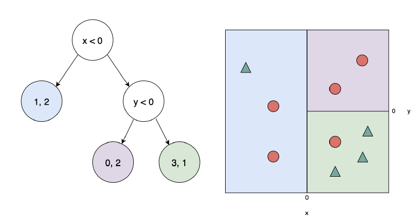
Figure 1: An example decision tree based on the features $x$ and $y$. Points with $x\geq 0$ and $y>0$ can be classified as one class (green triangles), whereas points in the other leaf nodes are classified as another (red circles).

Such DT ensemble methods are widely used in practice and improve upon individual DTs’ performance and stability. However, these methods lose their simplicity and interpretability. For these reasons, Bayesian CART (BCART) Model Search was proposed as an alternative to greedy DT construction algorithms for constructing individual DTs. BCART is a probabilistic method that assigns a prior probability distribution over the set of potential trees and updates the corresponding posterior distribution given the data. Individual trees generated by BCART, which we call Bayesian Decision Trees (BDTs), have been shown to have performance commensurate with that of entire greedily-constructed RFs (Linero, 2017). Furthermore, the posterior generated by the BCART method can be used to quantify uncertainty in the tree selection process.

In the BCART formulation, each individual DT is sampled from the posterior distribution of trees given the data, typically using Markov chain Monte Carlo (MCMC) methods. These methods typically only permit local transitions between trees, such as growing or pruning trees by a single node (Chipman et al., 1998; Denison et al., 1998). MCMC-based BCART methods have been shown to result in smaller and equally performant individual trees when compared with greedily constructed DTs and RF (Linero, 2017). Unfortunately, if the posterior over trees is naturally complex and multimodal, MCMC-based methods encounter long mixing times and exhibit mode collapse (Ronen et al., 2022; Yannotty et al., 2023). In practice, this often renders MCMC-based methods impractical.

Contributions: In this work, we propose a new Bayesian prior as a criterion for the Bayesian sampling objective when sampling decision trees. This criterion leads to an analytically tractable posterior distribution over trees given the data. We propose BCART-PCFG to sample from this posterior; BCART-PCFG is able to sample trees efficiently. At the heart of our method is a theoretical connection between our choice of prior and sampling from a probabilistic context-free grammar. Sampled trees demonstrate performance comparable to or better than existing, greedily-constructed trees, and are often significantly smaller. Furthermore, the sampling procedure is easily parallelizable and BCART-PCFG has only a single hyperparameter, which makes hyperparameter tuning simple.

2 Related Work

DTs are a popular for their strong out-of-the-box performance; DTs still outperform neural network approaches on tabular data (Grinsztajn et al., 2022). Popular algorithms for greedily training DTs include CART (Breiman et al., 1984), ID3 (Quinlan, 1986), and C4.5 (Quinlan, 1996). Recently, other work has focused on using metaheuristics for the training criterion (Rivera-Lopez et al., 2022) or accelerating the training procedure via adaptive sampling (Tiwari et al., 2022).

BDTs were first introduced simultaneously in Denison et al. (1998) and Chipman et al. (1998). Both works propose a prior over tree structures and suggest sampling from the posterior via MCMC methods. Since these papers, most followup work on BDTs has focused on accelerating the sampling procedure, e.g., via particle filtering (Lakshminarayanan et al., 2013) or other methods (Geels et al., 2022), and extending capabilities to larger datasets (Denison et al., 2002).

Significant recent work demonstrates the advantages of Bayesian methods for generating tree ensembles as opposed to the greedy, algorithmic method; see Linero (2017) for a recent review. In this line of work, Matthew et al. (2015) shows promising results for Bayesian tree ensembles but stops short of a fully Bayesian approach; instead, they sample decision stumps greedily and grow these stumps with a Bayesian approach. Nuti et al. (2021) showed that what they call greedy modal tree (GMT) can match the performance of the best trees constructed by greedy splitting criteria. However, their approach only considers a posterior across single-level splits and greedily constructs trees from the top down using this metric.

One of the most successful applications of BDTs is in Bayesian Additive Regression Trees (BARTs) (Chipman et al., 2010), which generate multiple Bayesian decision trees in order to partition data for downstream tasks, and its extensions (Deshpande, 2022; Maia et al., 2022; Nuti et al., 2019). However, similar to BDTs, these approaches often suffer from mode collapse and large mixing times, often rendering them unusable (Ronen et al., 2022; Yannotty et al., 2023).

We note that our approach is inspired by connections to probabilistic context-free grammars (Johnson et al., 2007; Kim et al., 2019; Lieck & Rohrmeier, 2021; Pynadath & Wellman, 1998; Toutanova & Manning, 2002; Saranyadevi et al., 2021; Stolcke & Omohundro, 1994; Teichmann, 2016; Vazquez et al., 2022; Hwang et al., 2011). Our sampling approach is also inspired by recently developed methods in Generative Flow Networks (Bengio et al., 2022; Do et al., 2022; Pan et al., 2022; Zimmermann et al., 2022).

3 Preliminaries

We consider a dataset $X,Y$ of $n$ independent observations $(\textbf{x}^{(1)},y^{(1)}),\dots,(\textbf{x}^{(n)},y^{(n)})$. we focus on the classification setting for simplicity, though our results also apply to the regression setting. In classification, each vector $\textbf{x}^{(i)}$ consists of $d$ features $\textbf{x}=(x_{1},\dots,x_{d})$, and each label $y\in\{1,\dots,C\}$.

Throughout this work, we let $T$ denote a binary tree and let $b(T)$ denote the number of terminal (leaf) nodes of $T$. We let $M_{j}\in b(T)$ denote the terminal nodes of tree $T$ for $j=1,2,\ldots,b(T)$ and $N_{k}$ denote the non-terminal (internal) nodes of $T$ for $k=1,2,\ldots,b(T)-1$.

Each internal node $N_{k}$ of $T$ is associated with a splitting rule, denoted $s_{k}$, which can be written as the subset $\{x_{i}<v\}$ for some $v\in\mathbf{R}$. $\overline{s}$ denotes the negation of the splitting rule $s$ (e.g., if $s$ is $x_{1}<3$ then $\overline{s}$ is $x_{1}\geq 3$). Points satisfying the splitting rule of an internal node are sent to its left child node and all others (those that satisfy the complement) are sent to its right child node. This splitting process continues until these points reach a terminal node in $T$.

Each node of $T$ is also associated with a bounding box that is axis-aligned (in feature space) and determined by the splits performed in $T$ to reach $N$ from the root node, which itself is denoted by $N_{0}$. With a slight abuse of notation, we use $N$ to refer to a node or its associated bounding box, with the meaning clear from context. Similarly, we use $N\cap s$ and $N\cap\overline{s}$ to denote the children of $N$ created by splitting according to rule $s$, i.e., the left and right children of $N$ when it is split by rule $s$, respectively.

If, for example, a node $N_{4}$ has three ancestors $N_{0},N_{2},N_{3}$ in which it is in the left, right, and left subtrees of, respectively, then the bounding box associated with $N_{4}$ is $N_{0}\cap s_{0}\cap\overline{s_{2}}\cap s_{3}$.

We let $X_{N}$ and $Y_{N}$ or $X_{M}$ and $Y_{M}$ denote the datapoints and their associated labels, respectively, at an internal node $N$ or a terminal node $M$. Two bounding boxes are considered equivalent if they contain the same datapoints.

3.1 Probabilistic Context Free Grammars

We briefly recapitulate Probablistic Context-Free Grammars (PCFGs). PCFGs are formally defined as a tuple of five elements: the start symbol, a set of nonterminal symbols, a set of terminal symbols, a set of production rules, and the set of probabilities over those production rules. A derivation in a PCFG consists of recursively applying production rules to the start symbol. The probability of an ordered derivation occurring is equal to the product of the probabilities for the production rules applied to generate that derivation.

4 Bayesian Decision Trees and BCART-PCFG

A Bayesian Decision Tree (BDT) is a binary tree $T$ and parameter $\Theta=(\bm{\theta}_{1},\dots,\bm{\theta}_{b(T)})$ that parameterizes the distributions over labels $f(y|\bm{\theta}_{1},\dots,f(y|\bm{\theta}_{b(T)})$ in each of the terminal nodes. Each distribution $f(y|\bm{\theta}_{i})$ is a categorical distribution parameterized by $\theta_{i,1},\dots,\theta_{i,C}$ where each $\theta_{i,c}$ denotes the probability that a datapoint in terminal node $i$ is assigned label $c$. With this notation, we state the following theorem:

Theorem 4.1.

Assume that labels are drawn independently from their respective distributions conditioned on $T$ and $\Theta$. Further assume a Dirichlet prior across these distributions of labels, $\bm{\alpha}=(\alpha_{1},\dots,\alpha_{C})$. Then the likelihood for dataset labels $Y$ given the predictors $X$ and binary tree $T$ is

$$\Pr[Y\mid X,T]=\prod_{j=1}^{b(T)}\frac{\beta(\mathbf{n_{j}}+\bm{\alpha})}{\beta(\bm{\alpha})}$$ (1)

where $\mathbf{n_{j}}=(n_{j,1},\dots,n_{j,C})$ is a vector where the $c$th coordinate is the number of occurrences of label $c$ in the $j$th terminal node, $\beta$ is the $C$-beta function given by

$$\beta(\gamma_{1},\dots,\gamma_{C})=\frac{\prod_{i=1}^{C}\Gamma(\gamma_{i})}{\Gamma\left(\sum_{i=1}^{C}\gamma_{i}\right)},$$ (2)

and $\Gamma$ is the gamma function given by $\Gamma(n)=(n-1)!$ for integer $n$.

Proof.

By the independence assumption, we may write

$$\Pr[Y|X,T]=\prod_{i=1}^{n}\Pr[y_{i}|x_{i},T].$$ (3)

Furthermore, by grouping the terms in the product on the right hand side by leaf node, we may write

$$\prod_{i=1}^{n}\Pr[y_{i}|x_{i},T] =\prod_{j=1}^{b(T)}\prod_{r=1}^{n_{j}}\int_{\bm{\theta}}\Pr[y_{i}|\bm{\theta}_{j},x_{i},T]\Pr[\bm{\theta}_{j}]d\bm{\theta}_{j}$$ (4)

$$=\prod_{j=1}^{b(T)}\prod_{r=1}^{n_{j}}\int_{\bm{\theta}}\Pr[y_{i}|\bm{\theta}_{j}]\Pr[\bm{\theta}_{j}]d\bm{\theta}_{j}$$ (5)

where $n_{j}$ is the number of datapoints in leaf $j$ of tree $T$ and since $Pr[y_{i}|\bm{\theta}_{j},x_{i},T]=Pr[y_{i}|\bm{\theta}_{j}]$ as the prediction $y_{i}$ only depends on the parameter $\bm{\theta}_{j}$. Furthermore,

$$\prod_{r=1}^{n_{j}}\int_{\bm{\theta}}\Pr[y_{i}|\bm{\theta}_{j}]\Pr[\bm{\theta}_{j}]d\bm{\theta}_{j} =\int_{\bm{\theta}}\prod_{r=1}^{n_{j}}\Pr[y_{i}|\bm{\theta}_{j}]\Pr[\bm{\theta}_{j}]d\bm{\theta}_{j}$$ (6)

$$=\frac{\beta(\mathbf{n_{j}}+\bm{\alpha})}{\beta(\bm{\alpha})}$$ (7)

for each $j$, where we used the fact that $\Pr[\bm{\theta}_{j}]\propto\theta_{j,1}^{\alpha_{1}-1}\ldots\theta_{j,C}^{\alpha_{C}-1}$ and results from (Denison et al., 1998). Thus

$$\Pr[Y|X,T]=\prod_{j=1}^{b(T)}\frac{\beta(\mathbf{n_{j}}+\bm{\alpha})}{\beta(\bm{\alpha})}$$ (8)

as desired. ∎

Theorem 4.1 allows us to compute the the likelihood of labels $Y$ occurring for data $X$ under a given tree structure $T$ and choice of leaf node probability distributions $f(y|\bm{\theta}_{1}),\dots,f(y|\bm{\theta}_{b(T)})$ where each $f$ is a Dirichlet distribution parameterized by its corresponding $\bm{\theta}$. For example, with the tree $T$ and points in Figure 1, assuming a uniform prior where $\bm{\alpha}=(1,1)$, the conditional likelihood $\Pr[Y|X,T]$ of generating the provided labels is $\frac{\beta(2,3)\beta(1,3)\beta(4,2)}{\beta(1,1)^{3}}$.

Our goal, however, is to sample trees from the posterior $\Pr[T\mid X,Y]$. To do so, we must also choose a prior across trees $\Pr[T|X]$. As noted in previous work (Buntine, 1992), the support of this distribution will depend on our data $X$ due to the following natural constraints, which we call the Tree Constraints:

1. the bounding boxes of nodes in $T$ must be nonempty, and

2. any splits on a node which result in the same two divided bounding boxes are considered equivalent.

These constraints significantly reduce the considered space of trees considered. In particular, the number of possible trees is finite.

We use a basic prior mentioned in previous work (Denison et al., 1998; Chipman et al., 1998) which scales exponentially with the number of terminal nodes in the tree. This choice of prior biases the tree search towards smaller trees:

$$\Pr[T\mid X]\propto\phi^{-b(T)}$$ (9)

Theorem 4.2.

The posterior over trees resulting from the likelihood in Equation (1) and prior in Equation (9) is:

$$\Pr[T\mid X,Y]\propto\left(\prod_{k=1}^{b(T)}\frac{\beta(\mathbf{n_{k}}+\bm{\alpha})}{\beta(\bm{\alpha})}\right)\left(\phi^{-b(T)}\right)$$ (10)

Proof.

A straightforward application of Bayes’ rule yields

$$\Pr[T\mid X,Y] \propto\Pr[Y\mid X,T]\Pr[T\mid X]$$ (11)

$$=\left(\prod_{k=1}^{b(T)}\frac{\beta(\mathbf{n_{k}}+\bm{\alpha})}{\beta(\bm{\alpha})}\right)\left(\phi^{-b(T)}\right)$$ (12)

∎

Theorem 4.2 provides us with a posterior for the trees given the data. In later sections, we will define a method of sampling trees according to this posterior.

5 Methodology

5.1 Bounding Box Score

Let $S(N)$ denote the set of splits of the form $s=\{x_{i}<d\}$ such that $N\cap s$ and $N\cap\overline{s}$ result in two nonempty bounding boxes. As before, we let any two such splits that result in the same two bounding boxes be considered equivalent. $S(N)$ contains one representative from each equivalence class.

We define the score of a bounding box to be:

$$Q(N)\coloneqq L(N)+\frac{1}{\phi}\sum_{s\in S(N)}Q(N\cap s)Q(N\cap\overline{s})$$ (13)

where $L(N)\coloneqq\Pr[Y_{N}|X_{N},\odot]$ is the likelihood of assigning the labels of $Y_{N}$ given an empty tree $\odot$. From Theorem 4.1, we have

$$L(N)=\frac{\beta(\bm{n}(N)+\bm{\alpha})}{\beta(\bm{\alpha})}$$ (14)

where $\bm{n}(N)\in\mathbf{R}^{C}$ represents the number of datapoints of each category in bounding box $N$.

5.2 Probabilistic Context-Free Grammar of Bounding Boxes

Using the score function $Q$, we define a specific PCFG across bounding boxes called PCFG*. In PCFG*, the start symbol is outermost bounding box $N_{0}$ which contains all indices in our dataset. The non-terminal symbols of PCFG* are the bounding boxes associated with non-terminal nodes. The terminal symbols are the bounding boxes associated with terminal nodes. We define two productions rules for every non-terminal symbol, specified as follows:

• split rule: $N\rightarrow N\cap s,N\cap\bar{s}$

• stop rule: $N\rightarrow M$

Each split rule represents a division of one bounding box into two smaller non-empty bounding boxes. A stop rule represents a transition from a non-terminal bounding box to a terminal bounding box which contains the same points but will not split further. We define the probability of split production rule $N\rightarrow N\cap s,N\cap\overline{s}$ to be:

$$\Pr[N\rightarrow N\cap s,N\cap\overline{s}]=\frac{Q(N\cap s)Q(N\cap\overline{s})}{\phi Q(N)}$$ (15)

and the probability of a stop production rule $N\rightarrow M$ t as:

$$\Pr[N\rightarrow M]=\frac{L(N)}{Q(N)}$$ (16)

Note that a string derived by PCFG* represents an ordered set of bounding boxes; the parse tree of this string corresponds directly with a decision tree containing the same internal/terminal nodes and internal node splits. Furthermore, every decision tree satisfying the Tree Constraints can be represented by some such parse tree, and so there is a bijection between parse trees in PCFG* and decision trees, where each of the production rules in the tree map directly to a split rule of the corresponding internal node of the decision tree. We denote by $P_{T}$ the parse tree associated with decision tree $T$ under this bijection. The probability that PCFG* generates a particular parse tree $P_{T}$ or decision tree $T$ is the product of its production rule probabilities. We are now ready to state our main result:

Theorem 5.1.

The probability of a parse tree $P_{T}$ to be generated in PCFG* is

$$\Pr[P_{T}] =\Pr[T|X,Y]$$ (17)

$$\propto\left[\prod_{k=1}^{b(T)}\frac{\beta(\mathbf{n_{k}}+\bm{\alpha})}{\beta(\bm{\alpha})}\right]\left[\phi^{-b(T)}\right]$$ (18)

Proof.

Suppose tree $T$ is generated by a sequence of splits $s_{1},s_{2},\ldots,s_{t}$ where each $s_{i}$ operates on node $N_{i}$. Note that all the $N_{i}$’s are distinct nodes as each node can only be split once. Without loss of generality, assume splits $s_{1},s_{2},\ldots,s_{b}\neq\odot$ are the nonterminating splits and $s_{b+1}=\ldots=s_{t}=\odot$ are the terminating splits. The likelihood of $P_{T}$ being generated by the associated production rules in PCFG* are

$$Pr[P_{T}]$$ (19)

$$=\left(\prod_{q=1}^{b}\Pr[Q\rightarrow(Q\cap s_{q})(Q\cap\bar{s}_{q})]\right)$$ (20)

$$\hskip 50.0pt\times\left(\prod_{p=b+1}^{t}\Pr[Q\rightarrow(Q\cap s_{p})]\right)$$ (21)

$$=\left(\prod_{q=1}^{b}\frac{Q(N_{q}\cap s_{q})Q(N_{q}\cap\bar{s}_{q})}{\phi Q(N_{q})}\right)$$ (22)

$$\hskip 50.0pt\times\left(\prod_{p=b+1}^{t}\frac{L(N_{p})}{Q(N_{p})}\right)$$ (23)

Note that every value $Q(N_{p})$ that appears in the denominator of the second product must appear exactly once in the numerator of the first product. Conversely, every term of the form $Q(N_{q}\cap s_{q})$ or $Q(N_{q}\cap\bar{s}_{q})$ in the numerator of the first product must appear exactly once in the denominator of the second product.

As such, the product telescopes and each $Q$ term cancels except for $Q(N_{0})$. We are left with

$$\Pr[P_{T}]=$$ (24)

$$\frac{\phi^{1-b(T)}}{Q(N_{0})}\left(\prod_{p=b+1}^{t}L(N_{p})\right)$$ (25)

$$\propto\phi\Pr[T|X]\left(\prod_{p=b+1}^{t}L(N_{p})\right)$$ (26)

$$\propto\Pr[T|X]\left(\prod_{p=b+1}^{t}L(N_{p})\right)$$ (27)

$$\propto\Pr[T|X]\prod_{\text{leaf nodes $M^{\prime}$ in $T$}}\Pr[Y_{M^{\prime}}|X_{M^{\prime}},\odot]$$ (28)

$$=\Pr[Y|X,T]\Pr[T|X]$$ (29)

$$\propto\Pr[T|Y,X]$$ (30)

where in the antepenultimate line we used that each $M_{p}$ is a terminal node and in the penultimate line we used independence of the labels in each leaf node conditioned on their corresponding datapoints.

Since $\Pr[P_{T}]\propto Pr[T|Y,X]$ and there is a bijection between the supports of each distribution, we must have $\Pr[P_{T}]=Pr[T|Y,X]$ under this same bijection. ∎

Theorem 5.1 states that to sample BDTs from our Bayesian objective $\Pr[T|X,Y]$, we can sample parse trees in PCFG*. The problem of sampling BDTs from $\Pr[T|X,Y]$ is thus reduced to sampling parse trees.

5.3 Computing Score

In order to sample from PCFG*, we must compute score function $Q$. Bounding boxes have a natural scoring given by the number of points they contain, which allows us compute their $Q$ values using dynamic programming naively in total time $O(n\cdot n^{2d})$ where $n$ is the total number of points in our dataset, $d$ is the number of features, and $O(n^{2d})$ is a loose upper bound on the number of bounding boxes. As a result, we see that Bayesian decision trees can be sampled directly from this posterior in linear time after polynomial time (in $n$, with $d$ fixed) precomputation of $Q$.

5.4 MAP Tree

The maximum a posteriori (MAP) decision tree can be also be discovered in a similar fashion. We define a modified score function $Q_{\max}$ as follows

$$Q_{\max}(N)=\max(L(N),\\ \frac{1}{\phi}\max_{s\in S(N)}Q_{\max}(N\cap s)Q_{\max}(N\cap\overline{s}).)$$

With a new PCFG defined using this score function, we can choose the rule with the highest probability recursively at each step. Algorithm 2 describes how to sample from the PCFG once $Q_{\max}$ has been computed.

5.5 Implicitly Generated Trees

Since predictions are made only on the terminal node in which a query falls within a decision tree, generating a full tree is not necessary for BCART-PCFG during inference. Instead, only the path to the terminal nodes specific to the provided query needs to be sampled.

Algorithm 1 Path Sample for Query Response

Input: Query point $q$
Output: Prediction $y$

1:  $N\leftarrow N_{0}$

2:  $terminal\leftarrow$ False

3:  while $terminal=$ False do

4:     Sample production rule $r$ according to the production rules probabilities in PCFG* for bounding box $N$

5:     if $r=N\rightarrow M$ then

6:        $N\leftarrow M$

7:        $terminal\leftarrow$ True

8:     else

9:        $s\leftarrow$ the production rule associated with split rule $r$

10:        if $q\in N\cap s$ then

11:           $N\leftarrow N\cap s$

12:        else

13:           $N\leftarrow N\cap\overline{s}$

14:        end if

15:     end if

16:  end while

17:  Draw prediction $y$ from $Pr[y|M]$

18:  return $y$

In this fashion, multiple paths can be sampled quickly to simulate the prediction of an ensemble of Bayesian Decision Trees sampled from the posterior. The exact query response of an ensemble across all supported trees can also be computed using dynamic programming in polynomial time. A similar method can also be used to determine the MAP tree’s response to future queries using the precomputed $Q_{\max}$ function.

Algorithm 2 Path Sample for Best Tree Query Response

Input: Query point $q$
Output: Prediction $y$

1:  $N\leftarrow N_{0}$

2:  $terminal\leftarrow$ False

3:  while $terminal=$ False do

4:     $s\leftarrow\frac{1}{\phi}$argmax${}_{s^{\prime}\in S(N)}Q_{\max}(N\cap s^{\prime})Q_{\max}(N\cap\bar{s^{\prime}})$

5:     if $L(N)>\frac{1}{\phi}Q_{\max}(N\cap s)Q_{\max}(N\cap\bar{s})$ then

6:        $N\leftarrow M$

7:        $terminal\leftarrow\text{True}$

8:     else

9:        if $q\in N\cap s$ then

10:           $N\leftarrow N\cap s$

11:        else

12:           $N\leftarrow N\cap\overline{s}$

13:        end if

14:     end if

15:  end while

16:  Draw prediction $y$ from $Pr[y|M]$

17:  return $y$

6 Experiments

6.1 Datasets:

We test the performance of BCART-PCFG and other baseline algorithms across one synthetic dataset and four real-world datasets from the UCI Machine Learning Repository (Dua & Graff, 2017). All datasets are approximately balanced.

XOR dataset: In the synthetic XOR dataset, each datapoint contains 20 features, each of which is a binary feature that is $1$ with probability $0.5$. The label for each datapoint is the 4-way XOR of the first four features. In this dataset, only the first four features are relevant to the label and the remaining 16 are not predictive of the label. A specific binary decision tree with 31 total nodes (16 leaf nodes, one for each possible value of the first four bits) should perfectly classify this dataset.

Iris dataset: The Iris dataset consists of 50 different samples of each of three different species of Iris flowers. Each datapoint has four dimensions: the length and width of the sepals and petals. The dataset presents a classification task with three possible labels, one corresponding to each species.

Caesarean Section dataset: The Caesarian Section dataset consists of data for 80 different pregnancies. Each pregnancy corresponds to a datapoint with five features: maternal age, delivery number, delivery time (early, timely, or late), blood pressure (low, normal, or high), and presence of heart problems. The dataset presents a classification task with two possible labels corresponding to whether a Caesarian section was performed for the delivery.

Haberman dataset: The Haberman dataset consists of data for 306 different patients who underwent surgery for breast cancer. Each patient corresponds to a datapoint with three features: patient age, year in which the surgery took place, and number of positive axillary nodes detected. The dataset presents a binary classification task corresponding to whether each patient survived for over 5 years post-surgery.

Vertebral Column dataset: The Vertebral Column dataset consists of data for 310 different orthopaedic patients. Each patient corresponds to a datapoint with six features corresponding to biomechanical attributes derived from the shape and orientation of the pelvis and lumbar spine: pelvic incidence, pelvic tilt, lumbar lordosis angel, sacral slope, pelvic radius, and grade of spondylolisthesis. The dataset presents a binary classification task corresponding to whether each patient displayed orthopaedic abnormalities.

Preprocessing: On all datasets, any features consisting of more than 10 distinct values were bucketed to 10 values. For the Vertebral Column dataset, feature values were bucketed to 5 values. No hyperparameter tuning was necessary for BDTs as ln$\phi$ was set to $2$, so no validation set was necessary. Hyperparameters for greedily-constructed trees were chosen to be their default values.

Testing: 10-fold cross validation was run and average accuracy was computed for each approach on all datasets.

Baselines: We compare the best BDT found by BCART-PCFG to the best DT found by greedy splitting (we call this the “single-best” setting). Additionally, we compare an ensemble of BDTs to RF (we call this the “ensemble” setting).

Metrics: We evaluate our algorithm against baselines by comparing two metrics: classification accuracy and tree size (number of total nodes). Higher accuracies and/or smaller tree sizes are better.

6.2 Results:

Across all datasets, BCART-PCFG performs either comparably to or better than RF in both the single-best and ensemble settings in accuracy. Additionally, BCART-PCFG produces consistently smaller models to achieve the same performance in both settings.

On the XOR dataset, we note BCART-PCFG is able to find trees that are of minimal size and achieve perfect classification accuracy. RF and the best single decision tree, however, are unable to perform as well, even though they construct significantly larger models. Inspection of greedily constructed DTs reveals that they often split on uninformative features, which increase model size without improving accuracy.

Dataset	Best CART	Best BCART-PCFG
Iris	0.967 ± 0.069	0.967 ± 0.092
Caesarian	0.525 ± 0.193	0.562 ± 0.311
Haberman	0.706 ± 0.219	0.719 ± 0.166
Vertebral	0.713 ± 0.167	0.716 ± 0.215
Hidden XOR	0.718 ± 0.217	1.0 ± 0.0

Table 1: Comparison of classification accuracies (%) for the best-performing CART tree and the best-performing BCART-PCFG tree on each dataset. Higher is better. On four of five datasets, BCART-PCFG outperforms CART. Means and 95% confidence intervals are obtained over 5 random trials.

Dataset	RF	BCART-PCFG Ensem.
Iris	0.96 ± 0.091	0.967 ± 0.092
Caesarian	0.55 ± 0.263	0.562 ± 0.289
Haberman	0.703 ± 0.197	0.716 ± 0.205
Vertebral	0.726 ± 0.191	0.732 ± 0.211
Hidden XOR	0.78 ± 0.121	1.0 ± 0.0

Table 2: Comparison of classification accuracies (%) for RF and an BCART-PCFG ensemble on each dataset. Higher is better. On all five datasets, BCART-PCFG outperforms CART. Means and 95% confidence intervals are obtained over 5 random trials.

Dataset	Best CART	Best BCART-PCFG
Iris	19.6 ± 4.153	7.0 ± 0.0
Caesarian	70.2 ± 2.024	3.2 ± 2.225
Haberman	161.0 ± 17.335	5.6 ± 3.227
Vertebral	106.2 ± 8.097	15.6 ± 4.545
Hidden XOR	392.2 ± 103.503	31.0 ± 0.0

Table 3: Comparison of model sizes (number of nodes) for the best-performing CART tree and the best-performing BCART-PCFG tree on each dataset. Smaller is better. On all five datasets, BCART-PCFG outperforms CART. Means and 95% confidence intervals are obtained over 5 random trials.

7 Conclusions and Limitations

Our results demonstrate that BCART-PCFG achieves similar performance to more common, greedily-constructed trees and constructs significantly smaller models. This suggests an application to compute-constrained hardware, such as embedded systems. We also note that BCART-PCFG is expected to excel on large datasets in which features interact to produce a label, such as the XOR dataset, because BCART-PCFG is able to do a global optimization over several splits rather than greedily splitting as in CART. A constraint of our work is that BCART-PCFG assumes a specific prior distribution over trees which allows us a subtree-decomposable objective function; while our experiments demonstrate this of prior works well in practice, other priors may be desirable in other settings. Future work will focus on discovering improved priors which fit into this framework. A further, significant limitation of our work is that our BCART-PCFG is restricted to datasets with small dimension due to the exponential scaling in $d$. In practice, it may be possible to perform some form of dimensionality reduction on the dataset to make BCART-PCFG feasible on high-dimensional datasets or to approximate the score function using machine learning methods. Since BCART-PCFG outperforms greedy decision-tree-generation methods when labels depend on more complex interaction between features, we anticipate such an extension of our work to higher-dimensional datasets would be valuable. Another significant constraint is that BCART-PCFG requires significant additional storage space compared to the greedy approach, and significantly larger training time for training only a small number (e.g., $1$) of trees. In practice, it may therefore be best to use BCART-PCFG in settings with significant computational resources (e.g., server-side) before providing the best single tree to more compute-constrained devices (e.g., smartphones).

References

- Bengio et al. (2022) Bengio, Y., Lahlou, S., Deleu, T., Hu, E. J., Tiwari, M., and Bengio, E. GFlowNet Foundations, August 2022. URL http://arxiv.org/abs/2111.09266. arXiv: 2111.09266 [cs, stat] Number: arXiv:2111.09266.
- Breiman (2001) Breiman, L. Random Forests. Machine learning, 45(1):5–32, 2001. Publisher: Springer.
- Breiman et al. (1984) Breiman, L., Friedman, J. H., Olshen, R. A., and Stone, C. J. Classification and Regression Trees. Chapman and Hall, 1 edition, 1984.
- Buntine (1992) Buntine, W. Learning Classification Trees. Statistics and Computing, 2(2):63–73, June 1992. ISSN 1573-1375. doi: 10.1007/BF01889584. URL https://doi.org/10.1007/BF01889584.
- Chen & Guestrin (2016) Chen, T. and Guestrin, C. XGBoost: A Scalable Tree Boosting System. In Proceedings of the 22nd ACM SIGKDD international conference on knowledge discovery and data mining, KDD ’16, pp. 785–794, New York, NY, USA, 2016. Association for Computing Machinery. ISBN 978-1-4503-4232-2. doi: 10.1145/2939672.2939785. URL https://doi.org/10.1145/2939672.2939785.
- Chipman et al. (1998) Chipman, H. A., George, E. I., and McCulloch, R. E. Bayesian CART Model Search. Journal of the American Statistical Association, 93(443):935–948, September 1998. ISSN 0162-1459. doi: 10.1080/01621459.1998.10473750. URL https://doi.org/10.1080/01621459.1998.10473750. Publisher: Taylor & Francis.
- Chipman et al. (2010) Chipman, H. A., George, E. I., and McCulloch, R. E. BART: Bayesian Additive Regression Trees. The Annals of Applied Statistics, 4:266–298, March 2010. ISSN 1932-6157. doi: 10.1214/09-AOAS285. arXiv: 0806.3286 [stat].
- Denison et al. (1998) Denison, D. G. T., Mallick, B. K., and Smith, A. F. M. A Bayesian CART Algorithm. Biometrika, 85(3):363–377, June 1998. ISSN 0006-3444. doi: 10.1093/biomet/85.2.363. URL https://doi.org/10.1093/biomet/85.2.363.
- Denison et al. (2002) Denison, D. G. T., Adams, N. M., Holmes, C. C., and Hand, D. J. Bayesian Partition Modelling. Computational Statistics & Data Analysis, 38(4):475–485, February 2002. ISSN 0167-9473. doi: 10.1016/S0167-9473(01)00073-1. URL https://doi.org/10.1016/S0167-9473(01)00073-1.
- Deshpande (2022) Deshpande, S. K. A New BART Prior for Flexible Modeling with Categorical Predictors, November 2022. URL https://doi.org/10.48550/arXiv.2211.04459. arXiv: 2211.04459 [stat] Number: arXiv:2211.04459.
- Do et al. (2022) Do, A., Dinh, D., Nguyen, T., Nguyen, K., Osher, S., and Ho, N. Improving Generative Flow Networks with Path Regularization, September 2022. URL http://arxiv.org/abs/2209.15092. arXiv: 2209.15092 [cs, stat] Number: arXiv:2209.15092.
- Dua & Graff (2017) Dua, D. and Graff, C. UCI machine learning repository, 2017. URL http://archive.ics.uci.edu/ml.
- Geels et al. (2022) Geels, V., Pratola, M. T., and Herbei, R. The Taxicab Sampler: MCMC for Discrete Spaces with Application to Tree Models. Journal of Statistical Computation and Simulation, pp. 1–22, September 2022. ISSN 0094-9655. doi: 10.1080/00949655.2022.2119972. URL https://doi.org/10.1080/00949655.2022.2119972. Publisher: Taylor & Francis.
- Grinsztajn et al. (2022) Grinsztajn, L., Oyallon, E., and Varoquaux, G. Why do Tree-Based Models Still Outperform Deep Learning on Tabular Data?, July 2022. URL https://doi.org/10.48550/arXiv.2207.08815.
- Hwang et al. (2011) Hwang, I., Stuhlmüller, A., and Goodman, N. D. Inducing Probabilistic Programs by Bayesian Program Merging, October 2011. URL https://doi.org/10.48550/arXiv.1110.5667. arXiv: 1110.5667 [cs] Number: arXiv:1110.5667.
- Johnson et al. (2007) Johnson, M., Griffiths, T., and Goldwater, S. Bayesian inference for PCFGs via Markov Chain Monte Carlo. In Main Proceedings of the Conference of the North American Chapter of the Association for Computational Linguistics, pp. 139–146, Rochester, New York, April 2007. Association for Computational Linguistics. URL https://aclanthology.org/N07-1018.
- Ke et al. (2017) Ke, G., Meng, Q., Finley, T., Wang, T., Chen, W., Ma, W., Ye, Q., and Liu, T.-Y. LightGBM: A Highly Efficient Gradient Boosting Decision Tree. In Guyon, I., Luxburg, U. V., Bengio, S., Wallach, H., Fergus, R., Vishwanathan, S., and Garnett, R. (eds.), Advances in Neural Information Processing Systems, volume 30. Curran Associates, Inc., December 2017. URL https://proceedings.neurips.cc/paper/2017/file/6449f44a102fde848669bdd9eb6b76fa-Paper.pdf.
- Kim et al. (2019) Kim, Y., Dyer, C., and Rush, A. Compound Probabilistic Context-Free Grammars for Grammar Induction. In Proceedings of the 57th Annual Meeting of the Association for Computational Linguistics, pp. 2369–2385, Florence, Italy, 2019. Association for Computational Linguistics. doi: 10.18653/v1/P19-1228. URL https://www.aclweb.org/anthology/P19-1228.
- Lakshminarayanan et al. (2013) Lakshminarayanan, B., Roy, D., and Whye Teh, Y. Top-Down Particle Filtering for Bayesian Decision Trees. In Dasgupta, S. and McAllester, D. (eds.), Proceedings of the 30th international conference on machine learning, volume 28 of Proceedings of machine learning research, pp. 280–288, Atlanta, Georgia, USA, June 2013. PMLR. URL https://proceedings.mlr.press/v28/lakshminarayanan13.html.
- Lieck & Rohrmeier (2021) Lieck, R. and Rohrmeier, M. Recursive Bayesian Networks: Generalising and Unifying Probabilistic Context-Free Grammars and Dynamic Bayesian Networks. Advances in Neural Information Processing Systems, 34:4370–4383, November 2021. URL https://www.semanticscholar.org/paper/Recursive-Bayesian-Networks%3A-Generalising-and-and-Lieck-Rohrmeier/25da1671548dc9a1e69d2e891a320b3335f909fd.
- Linero (2017) Linero, A. R. A Review of Tree-Based Bayesian Methods. Communications for Statistical Applications and Methods, 24(6):543–559, November 2017. ISSN 2383-4757. doi: 10.29220/CSAM.2017.24.6.543. URL http://www.csam.or.kr/journal/view.html?doi=10.29220/CSAM.2017.24.6.543.
- Maia et al. (2022) Maia, M., Murphy, K., and Parnell, A. C. GP-BART: A Novel Bayesian Additive Regression Trees Approach Using Gaussian Processes, December 2022. arXiv: 2204.02112 [cs, stat] Number: arXiv:2204.02112.
- Matthew et al. (2015) Matthew, T., Chen, C.-S., Yu, J., and Wyle, M. Bayesian and Empirical Bayesian Forests. In Bach, F. and Blei, D. (eds.), Proceedings of the 32nd international conference on machine learning, volume 37 of Proceedings of machine learning research, pp. 967–976, Lille, France, July 2015. PMLR. URL https://proceedings.mlr.press/v37/matthew15.html.
- Nuti et al. (2019) Nuti, G., Jiménez Rugama, L. A., and Thommen, K. Adaptive Bayesian Reticulum, December 2019. URL https://doi.org/10.48550/arXiv.1912.05901.
- Nuti et al. (2021) Nuti, G., Jiménez Rugama, L. A., and Cross, A.-I. An Explainable Bayesian Decision Tree Algorithm. In Frontiers in Applied Mathematics and Statistics, volume 7, pp. 598833, March 2021. ISBN 2297-4687. doi: 10.3389/fams.2021.598833. URL https://www.frontiersin.org/articles/10.3389/fams.2021.598833/full.
- Pan et al. (2022) Pan, L., Zhang, D., Courville, A., Huang, L., and Bengio, Y. Generative Augmented Flow Networks, October 2022. URL http://arxiv.org/abs/2210.03308. arXiv: 2210.03308 [cs] Number: arXiv:2210.03308.
- Pynadath & Wellman (1998) Pynadath, D. and Wellman, M. Generalized Queries on Probabilistic Context-Free Grammars. IEEE Transactions on Pattern Analysis and Machine Intelligence, 20(1):65–77, January 1998. ISSN 1939-3539. doi: 10.1109/34.655650.
- Quinlan (1986) Quinlan, J. R. Induction of Decision Trees. Machine Learning, 1(1):81–106, March 1986. ISSN 0885-6125, 1573-0565. doi: 10.1007/BF00116251. URL http://link.springer.com/10.1007/BF00116251.
- Quinlan (1996) Quinlan, J. R. Improved Use of Continuous Attributes in C4.5. Journal of Artificial Intelligence Research, 4:77–90, March 1996. doi: 10.1613/jair.279.
- Rivera-Lopez et al. (2022) Rivera-Lopez, R., Canul-Reich, J., Mezura-Montes, E., and Cruz-Chávez, M. A. Induction of Decision Trees as Classification Models Through Metaheuristics. Swarm and Evolutionary Computation, 69:101006, 2022. ISSN 2210-6502. doi: https://doi.org/10.1016/j.swevo.2021.101006. URL https://www.sciencedirect.com/science/article/pii/S2210650221001681.
- Ronen et al. (2022) Ronen, O., Saarinen, T., Tan, Y. S., Duncan, J., and Yu, B. A Mixing Time Lower Bound for a Simplified Version of BART, October 2022. URL https://doi.org/10.48550/arXiv.2210.09352.
- Saranyadevi et al. (2021) Saranyadevi, S., Murugeswari, R., and Bathrinath, S. A Context-free Grammar based Association Rule Mining Technique for Network Dataset. Journal of Physics: Conference Series, 1767(1):012007, February 2021. ISSN 1742-6588, 1742-6596. doi: 10.1088/1742-6596/1767/1/012007.
- Stolcke & Omohundro (1994) Stolcke, A. and Omohundro, S. Inducing Probabilistic Grammars by Bayesian Model Merging. In Carrasco, R. C. and Oncina, J. (eds.), International Colloquium on Grammatical Inference, volume 862, pp. 106–118, Berlin, Heidelberg, 1994. Springer Berlin Heidelberg. ISBN 978-3-540-48985-6. doi: 10.1007/3-540-58473-0˙141.
- Teichmann (2016) Teichmann, M. Expressing Context-Free Tree Languages by Regular Tree Grammars. Ph.D. dissertation, Technical University of Dresden, Dresden, Germany, October 2016. URL http://nbn-resolving.de/urn:nbn:de:bsz:14-qucosa-224756.
- Tin Kam Ho (1995) Tin Kam Ho. Random Decision Forests. In Proceedings of 3rd International Conference on Document Analysis and Recognition, volume 1, pp. 278–282, Montreal, Que., Canada, August 1995. IEEE Comput. Soc. Press. ISBN 978-0-8186-7128-9. doi: 10.1109/ICDAR.1995.598994. URL http://ieeexplore.ieee.org/document/598994/.
- Tiwari et al. (2022) Tiwari, M., Kang, R., Lee, J., Piech, C. J., Shomorony, I., Thrun, S., and Zhang, M. J. MABSplit: Faster Forest Training Using Multi-Armed Bandits. In Advances in Neural Information Processing Systems, October 2022. URL https://openreview.net/forum?id=yHFATHaIDN.
- Toutanova & Manning (2002) Toutanova, K. and Manning, C. D. Feature Selection for a Rich HPSG Grammar Using Decision Trees. In Proceedings of the 6th Conference on Natural Language Learning, volume 20, pp. 1–7. Association for Computational Linguistics, August 2002. doi: 10.3115/1118853.1118883.
- Vazquez et al. (2022) Vazquez, H. C., Sánchez, J. A., and Carrascosa, R. GramML: Exploring Context-Free Grammars with Model-Free Reinforcement Learning. In Sixth Workshop on Meta-Learning at the Conference on Neural Information Processing Systems, October 2022. URL https://openreview.net/forum?id=OpdayUqlTG.
- Yannotty et al. (2023) Yannotty, J. C., Santner, T. J., Furnstahl, R. J., and Pratola, M. T. Model Mixing Using Bayesian Additive Regression Trees, January 2023. URL http://arxiv.org/abs/2301.02296. arXiv: 2301.02296 [stat] Number: arXiv:2301.02296.
- Zimmermann et al. (2022) Zimmermann, H., Lindsten, F., van de Meent, J.-W., and Naesseth, C. A. A Variational Perspective on Generative Flow Networks, October 2022. URL http://arxiv.org/abs/2210.07992. arXiv: 2210.07992 [cs, stat] Number: arXiv:2210.07992.