Score-based Diffusion Models in Function Space

Abstract

Diffusion models have recently emerged as a powerful framework for generative modeling. They consist of a forward process that perturbs input data with Gaussian white noise and a reverse process that learns a score function to generate samples by denoising. Despite their tremendous success, they are mostly formulated on finite-dimensional spaces, e.g., Euclidean, limiting their applications to many domains where the data has a functional form, such as in scientific computing and 3D geometric data analysis. This work introduces a mathematically rigorous framework called Denoising Diffusion Operators (DDOs) for training diffusion models in function space. In DDOs, the forward process perturbs input functions gradually using a Gaussian process. The generative process is formulated by integrating a function-valued Langevin dynamic. Our approach requires an appropriate notion of the score for the perturbed data distribution, which we obtain by generalizing denoising score matching to function spaces that can be infinite-dimensional. We show that the corresponding discretized algorithm generates accurate samples at a fixed cost independent of the data resolution. We theoretically and numerically verify the applicability of our approach on a set of function-valued problems, including generating solutions to the Navier-Stokes equation viewed as the push-forward distribution of forcings from a Gaussian Random Field (GRF), as well as volcano InSAR and MNIST-SDF.

Keywords: Diffusion models, Score matching, Generative models, Operator learning, Function spaces

1 Introduction

Diffusion models (DMs) (Song et al., 2020b; Ho et al., 2020; Sohl-Dickstein et al., 2015) have appeared as a highly successful generative approach for various domains, including images (Saharia et al., 2022), 3D data (Poole et al., 2022), audio (Kong et al., 2020), video (Voleti et al., 2022a), machine learning security (Nie et al., 2022), natural language (Li et al., 2022), proteins (Wu et al., 2022), and molecules (Xu et al., 2022). These models consist of two processes: A forward diffusion process that corrupts input data by gradually adding white noise and a reverse generative process that proceeds by iterative denoising.

Typically, DMs operate on a finite-dimensional space, e.g. $\mathbb{{R}}^{n}$, limiting their application in domains where the data is represented by infinite-dimensional objects, e.g. continuous functions. For example, in weather forecasting, data samples are functions of temperature, pressure, and wind, defined on the surface of the globe (Pathak et al., 2022). This also extends to seismology, geophysics, oceanography, aerodynamic vehicle design, and fluid dynamics, where we interact with functional data governed by partial differential equations (PDE) (Yang et al., 2021; Wen et al., 2023). Additionally, in 3D vision and graphics applications, data is represented as functions in the form of radiance fields (Mildenhall et al., 2021) or signed distance functions (SDF) (Park et al., 2019).

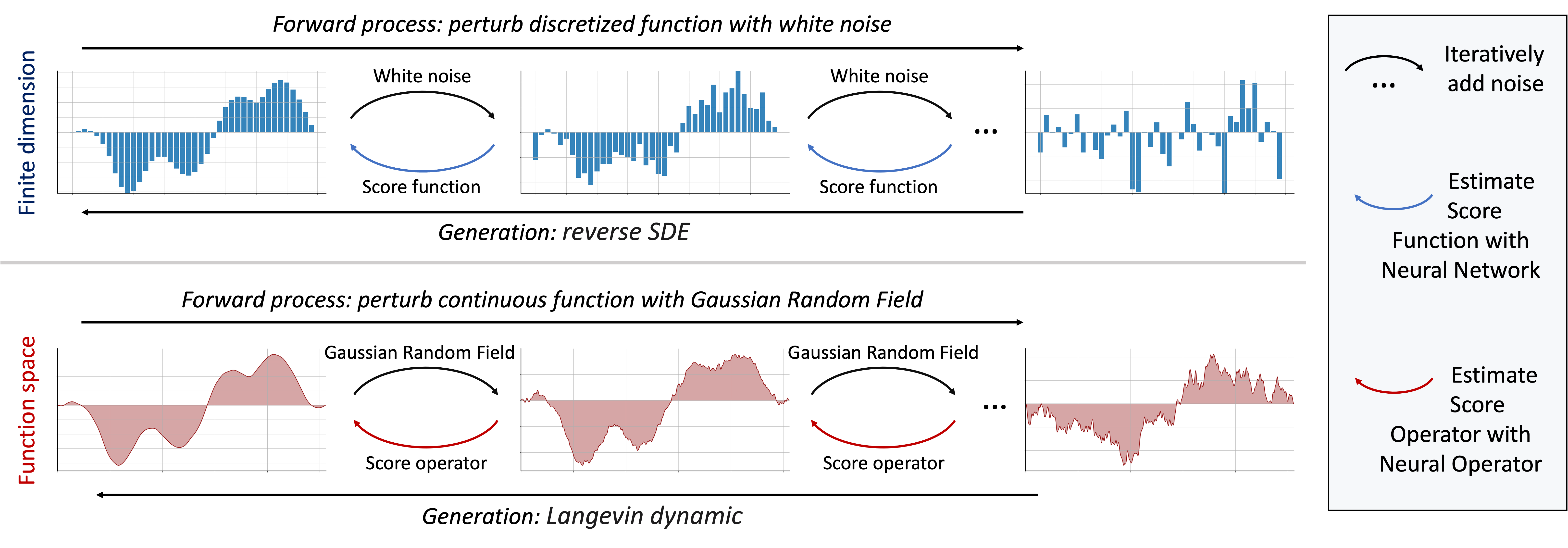
Figure 1: Overview of our approach. While in the finite-dimensional case, inputs are discretized, we work directly in function space, on continuous inputs, here 1D functions on $\mathbb{{R}}$. Noise is first added to the training samples during the forward process. A Neural Operator is used to estimate a score operator (Sec. 4) by minimizing the simplified loss in Eq. (12). Samples are generated using Langevin dynamics (Sec. 4.1). Using structured noise enables efficient learning in function space while white noise does not as the model capacity required grows with the resolution.

Recent attempts at applying DMs to functional data can be grouped into two categories: (i) the application of established algorithms on a discretization of functional data on $\mathbb{{R}}^{n}$ i.e. conditioning on point-wise values. While this approach can be made to work well at a fixed discretization, the models do not immediately transfer to variable discretizations of the data, and will not scale to higher resolutions (Dutordoir et al., 2022; Zhou et al., 2021), (ii) the mapping of input functions to a finite-dimensional latent space and modeling the latent embedding of the data with DMs (Dupont et al., 2022; Phillips et al., 2022; Hui et al., 2022; Bautista et al., 2022; Chou et al., 2022). Such approaches rely on efficient transformations of the data into compactly representable spaces, which limits their general applicability and are not guaranteed to be discretization-independent/convergent (Kovachki et al., 2021b).

The recently proposed infinite-dimensional diffusion model in Kerrigan et al. (2022) is closely related to our work. They consider a Gaussian noise corruption process in Hilbert space and derive a loss function to approximate the conditional mean of the reverse process. While the loss function is formulated using infinite-dimensional measures, the difference between the true and approximate means does not satisfy the strict range conditions that are required to have non-singular measures, and thus yields a loss that is almost surely infinite. Numerically, this effect can only be seen through progressive grid refinement which the work does not consider. For further discussion, see Appendix H.

Developing a diffusion-based generative framework for functions requires solving several technical challenges. First, instead of the commonly used Gaussian white noise, a new function-valued corruption process must be introduced to gradually map the data functions into random functions. Second, sample generation requires an appropriate notion of the score since infinite-dimensional distributions do not have standard probability density functions (pdf). Finally, approximating the score requires both careful analysis and generalization of finite-dimensional techniques in order to obtain a well-defined optimization problem as well as approximation architectures that are consistent as mappings between function spaces.

In our approach, we introduce a rigorous framework termed denoising diffusion operators (DDOs) that addresses these challenges. DDOs use a Hilbert space-valued Gaussian process to perturb the input data. To define an appropriate notion of the score, we first consider densities with respect to a Gaussian measure (as opposed to the Lebesgue measure). The derivative of this density for certain perturbations of the Gaussian measure defines the score operator. To approximate this score in practice, we generalize the denoising score matching objective of Vincent (2011) to our setting, and show how samples can be generated using Langevin dynamics with a learned score operator.

For learning the score, we utilize the neural operators (Li et al., 2020b, a; Kovachki et al., 2021b), which provide a consistent architecture in function space. We theoretically prove that approximating the score operator using neural operators is feasible. Figure 1 provides an overview of our approach. By working directly in the function space and discretizing only later for the purposes of computation, we obtain scalable and discretization-independent algorithms for generative models in function spaces.

Our primary contributions are summarized below:

1. We develop a mathematically rigorous framework for denoising score matching with function-valued data called DDO by formulating and extending all necessary theory to the abstract Hilbert space setting.

2. We propose a diffusion model for incrementally sampling from the data distribution by discretizing an infinite-dimensional Langevin equation with a hierarchy of noise corruption Gaussian processes, generalizing several popular finite-dimensional frameworks.

3. We empirically show DDO learns distributions of function-valued data on various datasets, including generating solutions to the Navier-Stokes equation viewed as the push-forward distribution of forcings from a Gaussian Random Field (GRF), as well as volcano Interferometric Synthetic Aperture Radar (InSAR) (Rosen et al., 2012) and MNIST-SDF (Sitzmann et al., 2020).

4. We empirically verify DDO’s invariance to spatial discretization with fixed model capacity, and demonstrate accurate sample generation of a non-Gaussian distribution from the pushforward of random forcings from a GRF under the Navier-Stokes solution operator.

2 Related Works

Our approach is broadly related to generative models formulated directly in function space instead of finite-dimensional Euclidean space (Rahman et al., 2022). Approaches for dealing with functional data include Gaussian processes (Rasmussen, 2004), and neural operators (Li et al., 2020b, a; Nelsen and Stuart, 2021). These methods aim to define deep learning models in function spaces, generalizing traditional neural networks.

In the context of generative diffusion models, this complication enters the model complexity and the number of time steps that typically need to grow with the data dimension. To improve sample quality and reduce the cost of sample generation in high dimensions, yet finite, several methods propose to use diffusion models in transformed spaces. These include latent spaces (Vahdat et al., 2021), hierarchically defined subspaces (Jing et al., 2022), spectral decompositions (Phillips et al., 2022), and extend to multi-scale wavelet transformations (Guth et al., 2022). Compared to score-based models operating in the original domain, the latter approach shows that the time complexity (i.e., the number of time steps required to achieve a fixed error) grows linearly with the image dimension. However, these models are not formulated in an infinite-dimensional space.

Neural Processes (NP) (Garnelo et al., 2018; Kim et al., 2019; Bruinsma et al., 2021) aim to model distributions consistent with arbitrary discretizations, and Dutordoir et al. (2022) have examined their extension to Neural Diffusion Processes (NDP). While the NP framework can process arbitrary sets of inputs, they inherit the limitations of using finite-dimensional latent variables; thus, consistency breaks in practice as the resolution grows. Moreover, the induced model distributions in NDP do not exist in function space due to independent noise in the noise process.

An earlier attempt to learn measures on function spaces deploys sequences of delta functions to fully memorize the data points (Craswell, 1965). Such a method is based on pure memorization and ignores possible underlying structures of the data measure. Kernel density estimation was proposed as a heuristic approach in infinite dimensional spaces (Dabo-Niang, 2004), though requires smoothness, extra regularity, and continuity with respect to an unspecified measure (Dabo-Niang, 2004). Alternative methods treat a discretized function as a point cloud and aim to maximize the likelihood of the point values (Garnelo et al., 2018), similarly to NPs.

Leveraging neural operators, Rahman et al. (2022) propose the generative adversarial neural operator (GANO) for learning function data distribution. As such, it learns a mapping between infinite dimension spaces, enabling learning of the distribution in function spaces. However, GANO  inherently suffers from the major drawbacks of adversarial training, such as limited stability, optimization, and flexibility, as pointed out in prior works (Arjovsky and Bottou, 2017; Lin et al., 2018; Song and Ermon, 2019; Berard et al., 2020).

The use of Gaussian Random Fields (GRFs) in denoising diffusion models has been discussed but is yet to be explored in the domain of function spaces (Voleti et al., 2022b). The generative adversarial neural network framework (Goodfellow et al., 2020) was recently used in conjunction with implicit neural network representations of data (Dupont et al., 2021; Anokhin et al., 2021; Skorokhodov et al., 2021; Chen et al., 2021). These methods are not discretization invariant and fail as the discretization of the data changes (Rahman et al., 2022). Dupont et al. (2022) embeds discretized data in function space using implicit neural network representations, but it still inherits the drawbacks of using finite-dimensional latent spaces to encode infinite-dimensional data.

Recently, continuous-time diffusion models in function space have also been proposed (Pidstrigach et al., 2023; Baldassari et al., 2023; Hagemann et al., 2023). These works define a forward and backward process by a pair of stochastic differential equations (SDEs) where the score operator is given as a conditional expectation, depending on the forward process. Our work offers an alternative viewpoint with the scored defined as a logarithmic derivative of a perturbed measure and sampling is done via a Langevin process. This allows us to make clearly interpretable assumptions on the data measure needed to guarantee convergence in the infinite-dimensional setting and furthermore allows us to study the interplay between the regularity of noise and the data.

3 Background: Denoising Score Matching in Finite Dimensions

Historically, score matching refers to the notion of approximating the score (i.e., the logarithmic derivative) of some unknown or computationally intractable distribution for the purposes of sampling, testing, or density estimation. Let $p\colon\mathbb{{R}}^{d}\to\mathbb{{R}}$ denote the pdf of a $d$-dimensional distribution and let $s_{\theta}:\mathbb{{R}}^{d}\to\mathbb{{R}}^{d}$ be a parametric mapping with parameters $\theta\in\mathbb{{R}}^{m}$. Ideally, score matching aims to solve

$$\min_{\theta\in\mathbb{{R}}^{p}}\mathbb{{E}}_{x\sim p(x)}\|s_{\theta}(x)-\nabla\log p(x)\|^{2}_{2}.$$ (1)

In many applications, we are only given samples from $p$, but do not know its analytic form. Therefore, solving (1) is intractable. Using integration by parts on the objective, Hyvärinen (2005) showed that the minimizer of (1) can be found by optimizing

$$\min_{\theta\in\mathbb{{R}}^{p}}\mathbb{{E}}_{x\sim p(x)}\left[\text{Tr}\big{(}\nabla s_{\theta}(x)\big{)}+\|s_{\theta}(x)\|^{2}_{2}\right].$$ (2)

Remarkably, the objective in (2) can be minimized using a Monte-Carlo approximation to the expectation. It was later noted in Vincent (2011) that, up to a perturbation of the data distribution, the optimization problem is equivalent to denoising score matching where the objective depends on the analytically tractable score of the conditional perturbed distribution and no derivatives of the approximating function. In particular, for a Gaussian perturbation of variance $\sigma^{2}$, (1) is equivalent to optimizing

$$\min_{\theta\in\mathbb{{R}}^{p}}\mathbb{{E}}_{\eta\sim N(0,\sigma^{2}I)}\mathbb{{E}}_{x\sim p(x)}\left\|\frac{\eta}{\sigma^{2}}+s_{\theta}(x+\eta)\right\|_{2}^{2},$$ (3)

where $s_{\theta}$ is now an approximation to the score of the perturbed distribution. Since (3) does not require knowledge of $p$ or computation of any derivatives, denoising score matching is attractive for problems in high dimensions where computing derivatives is costly. Furthermore, it is argued in Song and Ermon (2019), that for many practical applications, for example, photorealistic image generation, $p$ is supported on a lower dimensional manifold and thus approximating the score on the ambient space can be unstable. Thus perturbing the data distribution gives both a more computationally tractable optimization problem and acts as a regularizer by spreading the support of $p$ to the entire space.

We build on this framework by generalizing the notion of score and denoising score matching to infinite dimensions. By working directly in the infinite-dimensional setting, we derive a methodology that is consistent and generalizable across different discretizations of the data.

4 Denoising Diffusion Operators (DDO)

We introduce DDO to perform denoising score matching in function space. We work on an infinite-dimensional, real, separable Hilbert space $(H,\langle\cdot,\cdot\rangle,\|\cdot\|)$ with the Borel $\sigma$-algebra of measurable sets denoted $\mathcal{{B}}(H)$. Since there is no Lebesgue measure in infinite dimensions, there is no standard notion of a probability density; we therefore adopt the more general, measure-theoretic notation to introduce our setting. We denote by $\mu$ a probability measure on $\mathcal{{B}}(H)$ which we will call our data measure. In particular, we assume to have a dataset of samples $\{u_{j}\}_{j=1}^{N}$ where $u_{j}\sim\mu$ are i.i.d. random variables. These samples are considered to be infinite-dimensional objects, i.e. functions or infinite sequences, before any finite-dimensional discretization is done for the purposes of computation.

For a corruption process, we consider additive Gaussian perturbations to the data in the form of function-valued GRF perturbations. This choice is motivated by the availability of analytical results related to Gaussian measures, the ease and efficiency of sampling Gaussians in infinite dimensions by means of the Karhunen-Loéve expansion (Lord et al., 2014) (see Appendix G), and the plethora of empirically successful results for denoising score matching with Gaussians in finite dimensions (Song et al., 2020a; Ho et al., 2020). We employ the centered Gaussian measure on $H$ denoted by $\mu_{0}=N(0,C)$ with a covariance operator $C:H\to H$ to be self-adjoint, non-negative, and trace-class (nuclear). Indeed, these conditions on $C$ are necessary and sufficient for $\mu_{0}$ to be Gaussian on $H$ (Da Prato et al., 1992). We note that since trace-class implies compact, the identity covariance operator is ruled-out as $H$ is infinite-dimensional. In particular, white noise does not live in $H$ but must rather be defined on a larger space (Da Prato et al., 1992). We show empirically that by working with noise defined on $H$ our method remains discretizationally invariant with respect to the data. On the other hand, working with white noise breaks this property precisely because white noise samples are not regular compared to the elements of $H$.

We consider the perturbation to the data samples

$$v=u+\eta,\qquad u\sim\mu,\;\eta\sim\mu_{0},$$ (4)

with $u\perp\eta$ and denote by $\nu$ the probability measure induced by the random variable $v$ i.e. the convolution $\nu=\mu*\mu_{0}$; see Appendix B.1 for more details. We show in Lemma 9, that when the noise $\eta$ is small in an approximate sense, $\mu$ and $\nu$ are close as measures in the Wasserstein metric. It is therefore reasonable to approximate $\nu$ instead of $\mu$ as is done in denoising score matching since in the limit of vanishing noise, the two become identical.

We define the score of $\nu$ via an appropriate notion of density, which is defined with respect to a reference measure. In infinite dimensions, much work has been focused on studying densities defined with respect to Gaussian measures (as opposed to the Lebesgue measure in finite dimensions) as doing so has natural applications in statistics, inverse problems, and quantum field theory (Ghosal and van der Vaart, 2017; Stuart, 2010; Kupiainen, 2016). We also take this approach as it leads to a well-defined notion of the score that is analytically tractable and comes with an associated Langevin equation which can be solved to produce samples from $\nu$. We choose the reference to be perturbing measure $\mu_{0}$, which is natural in this setting since the conditional $v|u$ is Gaussian with the same covariance as $\mu_{0}$. A density is then be obtained by the Radon–Nikodym Theorem under the assumption that $\nu$ is absolutely continuous with respect to $\mu_{0}$, i.e., $\nu\ll\mu_{0}$ (Halmos, 1976).

To satisfy the absolute continuity condition with respect to Gaussian $\mu_{0}$, it is reasonable to expect that the data measure $\mu$ must satisfy certain assumptions. The assumption we make is that $\mu(H_{\mu_{0}})=1$, i.e., $\mu$ is fully supported on the Cameron-Martin space of $\mu_{0}$ that is denoted by $H_{\mu_{0}}\coloneqq C^{1/2}(H)$. Cameron-Martin spaces play a crucial role in the theory of Gaussian measures as they are an invariant of the measure that gives it meaning outside the ambient space $H$ (Bogachev, 2015). We remark that this assumption can make precise the manifold hypothesis in Song and Ermon (2019) that is used to justify the perturbation since $H_{\mu_{0}}$ is a proper subspace of $H$ and, in fact, $\mu_{0}(H_{\mu_{0}})=0$; see Section 6 of Stuart (2010) for more details. In particular, data samples lie on a measure-zero set of the perturbing measure. The addition of noise thereby spreads out the samples to the whole space. We note that when this assumption is not satisfied, we can still apply our framework using a different form of the perturbation in (4); see Section 4.3.

Under the condition above on the data perturbations, we can now state the following theorem.

Theorem 1 (Measure Equivalence)

The perturbed measure $\nu$ and the centered Gaussian $\mu_{0}$ are equivalent in the sense of measures, which we denote by $\nu\sim\mu_{0}$.

A more general statement and proof of this result are given in Appendix B.1. The importance of Theorem 1 is that it allows us to obtain a density. Indeed, it verifies the assumption of the Radon–Nikodym Theorem, which we apply to obtain a strictly positive density of $\nu$ with respect to $\mu_{0}$. In particular, there exists a Borel measurable mapping $\Phi\colon H\to\mathbb{{R}}$ such that

$$\frac{d\nu}{d\mu_{0}}(w)=\text{exp}\big{(}\Phi(w)\big{)},\qquad\mu_{0}\text{-a.s. }w\in H.$$ (5)

We will assume that $\Phi$ is Fréchet differentiable along the Cameron-Martin space $H_{\mu_{0}}$ which is itself a Hilbert space continuously embedded in $H$. This is a reasonable assumption since the vectors of differentiability of any Gaussian are precisely those in its Cameron-Martin space and $\nu$ is equivalent, in the sense of measures, to the Gaussian $\mu_{0}$ (Bogachev, 2015). While in finite dimensions differentiability is always ensured since Gaussians have infinitely smooth density and convolutions preserve this regularity, in infinite dimensions, this need not always be the case. We therefore make it an assumption, however, the following example shows that it is true of any Gaussian data measure.

Example 1

Suppose $\mu=N(0,Q)$ for some self-adjoint, non-negative, and trace-class operator $Q:H\to H$. It follows by non-negativity that

$$\langle h,Ch\rangle\leq\langle h,(C+Q)h\rangle\qquad\forall\>h\in H.$$

Therefore by Lemma 6.15 in (Stuart, 2010), $C^{1/2}(H)\subseteq(C+Q)^{1/2}(H)$. From definition $\nu=N(0,C+Q)$ and, by Proposition 5.1.6. in (Bogachev, 2015), $\nu$ is differentiable along its Cameron-Martin space $(C+Q)^{1/2}(H)$. Therefore $\nu$ is differentiable along $C^{1/2}(H)=H_{\mu_{0}}$.

We define the score precisely as the Fréchet derivative of $\Phi$ in the direction of $H_{\mu_{0}}$ and denote it $D_{H_{\mu_{0}}}\Phi\colon H\to H_{\mu_{0}}^{*}$ where $H_{\mu_{0}}^{*}$ is the topological (continuous) dual of $H_{\mu_{0}}$. In other words, the score of $\nu$ with respect to $\mu_{0}$ is the Fréchet derivative of the logarithm of the density of $\nu$ with respect to $\mu_{0}$,

$$D_{H_{\mu_{0}}}\Phi=D_{H_{\mu_{0}}}\log\frac{d\nu}{d\mu_{0}}.$$ (6)

We refer the reader to Chapter 5 in Bogachev (2015) for a general discussion of differentiability in infinite dimensions.

Having appropriately defined the score of $\nu$, we can introduce a score matching objective. Let $G_{\theta}\colon H\to H_{\mu_{0}}^{*}$ be a parametric mapping with parameters $\theta\in\mathbb{R}^{p}$. We consider the learning problem

$$\min_{\theta\in\mathbb{R}^{p}}\mathbb{{E}}_{v\sim\nu}\|D_{H_{\mu_{0}}}\Phi(v)-G_{\theta}(v)\|_{H^{*}_{\mu_{0}}}^{2}.$$ (7)

Since $D_{H_{\mu_{0}}}\Phi$ is unknown to us, solving (7) is computationally intractable.

To obtain a tractable problem, we generalize the conditioning theorem in Vincent (2011). Let us first notice that the measure induced by the conditional $v|u$ is the Gaussian $N(u,C)\coloneqq\gamma^{u}$ for $\mu$-almost any $u\in H$. Since $\mu(H_{\mu_{0}})=1$, the Feldman–Hájek Theorem implies that $\gamma^{u}\sim\mu_{0}$ (Da Prato et al., 1992). In particular, we may compute explicitly that, for $\mu_{0}\text{-almost any }w\in H$ and $\mu$-almost any $u\in H_{\mu_{0}}$,

$$\frac{d\gamma^{u}}{d\mu_{0}}(w) =\text{exp}\left(\sum_{j=1}^{\infty}\lambda_{j}^{-1}\langle w,\varphi_{j}\rangle\langle u,\varphi_{j}\rangle-\frac{1}{2}\|C^{-1/2}u\|^{2}\right)$$

$$\coloneqq\text{exp}\big{(}\Psi(w;u)\big{)},$$ (8)

where $C\varphi_{j}=\lambda_{j}\varphi_{j}$ for $j\in\mathbb{{N}}$ is an eigendecomposition of $C$ and $C^{-1/2}$ denotes the inverse of $C^{1/2}$ on $H_{\mu_{0}}$, see Theorem 2.23 in Da Prato et al. (1992). The score of each conditional $\gamma^{u}$ is given as the Fréchet derivative (in the first argument) of the potential $\Psi:H\times H_{\mu_{0}}\to\mathbb{{R}}$ in the direction of $H_{\mu_{0}}$. We can now state the following (informal) theorem relating (7) to the solution of a tractable problem.

Theorem 2 (Denoising Score Matching)

Under some integrability assumptions on $D_{H_{\mu_{0}}}\Phi$ and $G_{\theta}$, the minimizers of (7) are the same as the minimizers of

$$\min_{\theta}\mathbb{{E}}_{u\sim\mu}\mathbb{{E}}_{w\sim\gamma^{u}}\|D_{H_{\mu_{0}}}\Psi(w;u)-G_{\theta}(w)\|_{H_{\mu_{0}}^{*}}^{2}.$$ (9)

The more general statement (for a broader class of perturbations than (4)) and proof are given in Appendix B.2. Equation (9) gives us an infinite-dimensional analog of (3), where we can compute $D_{H_{\mu_{0}}}\Psi(w;u)$ from (4). That is,

$$D_{H_{\mu_{0}}}\Psi(w;u)=\sum_{j=1}^{\infty}\lambda_{j}^{-1}\langle u,\varphi_{j}\rangle\varphi_{j},$$ (10)

where we interpret (10) as

$$D_{H_{\mu_{0}}}\Psi(w;u)z=\sum_{j=1}^{\infty}\lambda_{j}^{-1}\langle z,\varphi_{j}\rangle\langle u,\varphi_{j}\rangle,$$ (11)

for any $z\in H_{\mu_{0}}$. Indeed, Lemma 11 shows that $D_{H_{\mu_{0}}}\Psi(w;u)\in H_{\mu_{0}}^{*}$ as defined by (10).

Recall that our objective is to approximate $D_{H_{\mu_{0}}}\Phi$ by solving (7), which we have shown is equivalent to (9). Given such an approximation, we can then solve a Langevin equation with the learned score in order to obtain samples from $\nu$. As we will show in the next section, this Langevin equation requires only knowledge of the $D_{H_{\mu_{0}}}\Phi$ projected onto $H_{\mu_{0}}$. We can thus simplify the optimization problem in (9) by considering the Reisz map $R:H_{\mu_{0}}^{*}\to H_{\mu_{0}}$, which is the canonical isometric isomorphism between the Hilbert spaces $H_{\mu_{0}}^{*}$ and $H_{\mu_{0}}$. Using the isometric property, we find

$$\|D_{H_{\mu_{0}}}\Psi(v;u)-G_{\theta}(v)\|_{H_{\mu_{0}}^{*}}^{2}=\|C^{-1/2}\big{(}u-RG_{\theta}(v)\big{)}\|^{2}$$

by noting that $R$ acts as $C$ to elements of $H_{\mu_{0}}^{*}$ that are not in $H_{\mu_{0}}$ and using (10). In particular, we have shown that minimizing (9) is equivalent to minimizing

$$\min_{\theta\in\mathbb{R}^{p}}\mathbb{{E}}_{u\sim\mu}\mathbb{{E}}_{\eta\sim\mu_{0}}\|C^{-1/2}\big{(}u-RG_{\theta}(u+\eta)\big{)}\|^{2},$$ (12)

which is a de-noising problem pre-conditioned by $C^{-1/2}$. Note that (12) is almost surely finite since $u-RG_{\theta}(w)\in H_{\mu_{0}}$ for any $w\in H$ by our assumption that $\mu(H_{\mu_{0}})=1$.

4.1 Langevin Dynamics

To sample from $\nu$, we consider the infinite-dimensional, pre-conditioned, Langevin equation,

$$\frac{du}{dt}=-u+RD_{H_{\mu_{0}}}\Phi(u)+\sqrt{2}\frac{dW}{dt},\quad u(0)=u_{0}$$ (13)

for some $u_{0}\in H$ where $RD_{H_{\mu_{0}}}\Phi:H\to H_{\mu_{0}}$ and W is a $C$-Wiener process (Da Prato et al., 1992). It is shown in Dashti and Stuart (2017) that, under appropriate boundedness assumptions on $RD_{H_{\mu_{0}}}\Phi$, equation (13) has a unique strong solution with continuous paths and an invariant measure $\nu$. In particular, samples from $\nu$ can be obtained as the long-time solutions of (13). We will approximate (13) by using the learned score $RG_{\theta}$ and discretizing in time using the Euler–Maruyama scheme with step-size $h>0$. This gives us the update

$$u_{n+1}=u_{n}+h(RG_{\theta}(u_{n})-u_{n})+\sqrt{2h}\xi_{n},$$ (14)

for any $n\in\mathbb{N}$ where $\xi_{n}\sim N(0,C)$ are i.i.d. random variables. Equation (14) also suggests that instead of looking for the map $RG_{\theta}$, we can re-parameterize and instead directly find the mapping $v\mapsto RG_{\theta}(v)-v$. To that end, suppose that $C$ is positive then $\text{ker}(C^{-1/2})=\{0\}$. Therefore, optimizing (12) is equivalent to optimizing

$$\min_{\theta\in\mathbb{R}^{p}}\mathbb{{E}}_{u\sim\mu}\mathbb{{E}}_{\eta\sim\mu_{0}}\|u-RG_{\theta}(u+\eta)\|^{2}.$$ (15)

Defining $F_{\theta}\colon H\to H$ by $F_{\theta}(v)=RG_{\theta}(v)-v$, we have

$$\min_{\theta\in\mathbb{R}^{p}}\mathbb{{E}}_{u\sim\mu}\mathbb{{E}}_{\eta\sim\mu_{0}}\|\eta+F_{\theta}(u+\eta)\|^{2},$$ (16)

which simplifies the sampling update in (14) to

$$u_{n+1}=u_{n}+hF_{\theta}(u_{n})+\sqrt{2h}\xi_{n}.$$ (17)

Note that this re-parameterization is only valid when $C$ is positive, otherwise (12) and (15) are not equivalent and $\text{Im}(F_{\theta})=H$ while $\text{dom}(C^{-1/2})=H_{\mu_{0}}$. In particular, for general $C$, we may optimize (12) and sample with (14), while for $C$ positive, we can alternatively optimize (16) and sample with (17). The advantage of (16) is that we can parameterize $F_{\theta}$ as an arbitrary $H\to H$ mapping without any restrictions on its range space. Furthermore current empirical evidence suggests that learning the noise from the signal instead of the signal from the noise yields better sample quality (Song and Ermon, 2020; Ho et al., 2020). Since $C$ is a choice in our method that can be tuned, we always pick it positive and thus utilize this re-parametrization in our experiments.

We remark that we have only picked the Euler–Maruyama discretization of (13) here for the sake of clarity in exposition. Many other choices such as Cotter et al. (2013) are possible; see Appendix D for details.

4.2 A Gaussian Example

We will now consider a simple example when the data measure is Gaussian to gain intuition on when we can expect the assumption $\mu(H_{\mu_{0}})=1$ to hold. Consider the space

$$H=\dot{L}^{2}(\mathbb{T}^{d};\mathbb{R})\coloneqq\left\{u\in L^{2}(\mathbb{T}^{d};\mathbb{R}):\int_{\mathbb{T}^{d}}u\>dx=0\right\},$$

where $\mathbb{T}^{d}$ is the $d$-dimensional unit torus. We denote by $\dot{H}^{s}(\mathbb{T}^{d};\mathbb{R})$ for any $s>0$ as the corresponding periodic, mean-zero Sobolev spaces (Adams and Fournier, 2003). Let $\mu=N(0,C_{1})$ where

$$C_{1}=\sigma_{1}^{2}(-\Delta+\tau_{1}^{2}I)^{-\alpha_{1}}.$$ (18)

Here $-\Delta$ is the negative Laplacian with periodic boundary conditions, $I$ is the identity operator, and $\sigma_{1},\tau_{1},\alpha_{1}$ are positive scalars. Covariances of the type (18) are said to be of the Matérn-type because Gaussian processes defined by Matérn kernels are the only stationary solutions to certain SPDEs with differential operator $C_{1}^{-1}$ (Whittle, 1954; Lindgren et al., 2011). We make extensive use of such covariances throughout the rest of this work as the Gaussian measures defined by them are amenable to analysis and efficient sampling. When $\alpha_{1}>d/2$, Lemma 6.27 in Stuart (2010) implies that $\mu\big{(}\dot{H}^{s}(\mathbb{T}^{d};\mathbb{R})\big{)}=1$ for any $s\in[0,\alpha_{1}-d/2)$. We will assume that $\alpha_{1}>d$. Let $\mu_{0}=N(0,C_{2})$ where

$$C_{2}=\sigma_{2}^{2}(-\Delta+\tau_{2}^{2}I)^{-\alpha_{2}}$$ (19)

with $\alpha_{2}>d/2$ so that $C_{2}$ is trace-class. It is easy to compute that $C_{2}^{1/2}(H)=\dot{H}^{\alpha_{2}}(\mathbb{T}^{d};\mathbb{R})$. Therefore, the assumption $\mu(H_{\mu_{0}})=1$ is satisfied for any $\alpha_{2}\in(d/2,\alpha_{1}-d/2)$.

The above analysis reveals that there is a gap of size $d/2$ between the regularity of the data and the noise. In particular, $\mu\big{(}\dot{H}^{s}(\mathbb{T}^{d};\mathbb{{R}})\big{)}=1$ for $s\in[0,\alpha_{1}-d/2)$ while $\mu_{0}\big{(}\dot{H}^{m}(\mathbb{T}^{d};\mathbb{{R}})\big{)}=1$ for $m\in[0,\alpha_{1}-d)$. Therefore, in order to consider perturbations with Gaussians of the form (4), the noise must be at least $d/2$ less smooth than the data, in a Sobolev sense. Furthermore since we want to consider noise with a trace-class covariance so that it is amenable to approximation, we have a fundamental limit on the regularity of the data. That is, the data must live in $\dot{H}^{s}(\mathbb{T}^{d};\mathbb{{R}})$ for some $s>d/2$. This assumption can be satisfied, for example, when the data measure is defined as the pushforward of some PDE solution operator; we show explicit examples in Appendix F.

4.3 Smoothing Operators

When the assumption $\mu(H_{\mu_{0}})=1$ is not satisfy, we may consider a different form of the perturbation in (4) to remove this regularity assumption. To that end, let $A\colon H\to H$ be a linear operator with the property that $A(H)\subseteq H_{\mu_{0}}$. Consider the data perturbation

$$v=Au+\eta,\qquad u\sim\mu,\;\eta\sim\mu_{0}.$$ (20)

We re-define the measures $\nu$ and $\gamma^{u}$ appropriately according to (20). Corollary 6 and the Feldman–Hájek Theorem imply that $\nu\sim\mu_{0}$ and $\gamma^{u}\sim\mu_{0}$ for $\mu$-almost every $u\in H$. Therefore the results of the previous section hold with the mapping $u\mapsto Au$ implemented in all formulae. Crucially, the learning problem in (12) becomes

$$\min_{\theta\in\mathbb{R}^{p}}\mathbb{{E}}_{u\sim\mu}\mathbb{{E}}_{\eta\sim\mu_{0}}\|Au-RG_{\theta}(Au+\eta)\|^{2},$$ (21)

while (16) becomes

$$\min_{\theta\in\mathbb{R}^{p}}\mathbb{{E}}_{u\sim\mu}\mathbb{{E}}_{\eta\sim\mu_{0}}\|\eta+F_{\theta}(Au+\eta)\|^{2}.$$ (22)

Here $A$ acts as a smoothing operator, bringing the data into a regular enough space for the required absolute continuity to hold. This makes mathematically precise diffusion models which use heat-dissipation or blurring as a forward operator (Rissanen et al., 2022; Hoogeboom and Salimans, 2022). We expand on this idea in the following section (See Appendix I).

4.4 Multiple Noise Scales

(a)

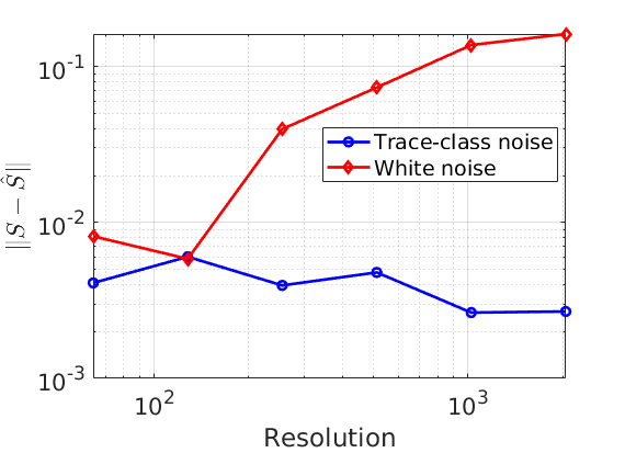
(a)

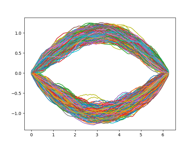
(b)

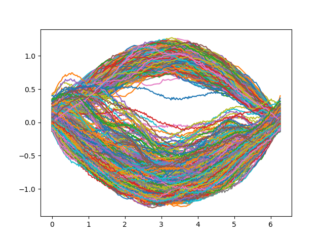
(c)

(a)

Figure 2: Gaussian mixture (Section 5.1): (a) Uniform-norm error in the average spectra of samples when using trace-class noise vs. white noise. (b) Generated samples at a resolution of 256 with trace-class noise and (c) with white noise.

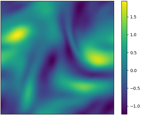
(a)

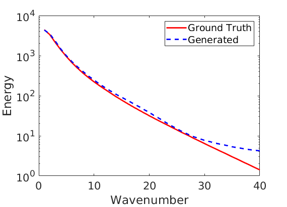
(b)

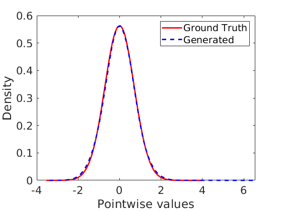
(c)

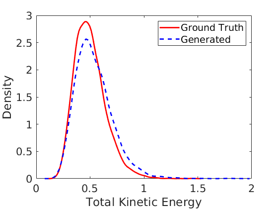
(d)

Figure 3: Navier-Stokes (Section 5.2): (a) Generated sample at the resolution $1024\times 1024$ with a model trained at $128\times 128$, (b) Spectrum, (c) Pointwise value density, (d) Total kinetic energy density of samples from the model vs. the data.

As argued in Song and Ermon (2019), the mixing times of Langevin dynamics such as (13) may be slow. It therefore of practical interest to consider multiple noise processes over different scales and thereby an annealing process for discretizing (13). To that end, let $\mathcal{{I}}$ be some (possibly uncountable) index set and consider the data perturbations

$$v_{t}=A_{t}u+\eta_{t},\qquad u\sim\mu,\;\eta_{t}\sim\mu_{t}$$ (23)

for a family of linear operators $\{A_{t}\colon H\to H\}_{t\in\mathcal{{I}}}$ and Gaussian measures $\{\mu_{t}\}_{t\in\mathcal{{I}}}$. Let $\nu_{t}$ be the measure for $v_{t}$.

Let us first consider the case $\mu_{t}=N(0,C_{t})$ where $C_{t}=g(t)C$ with $C$ as before, $A_{t}=f(t)I$ where $I$ is the identity operator, and $f,g:\mathcal{{I}}\to\mathbb{{R}}$ are mappings bounded from above and below away from zero. Lemma 12 shows that $A_{t}(H)\subseteq H_{\mu_{t}}$ for all $t\in\mathcal{{I}}$ and therefore our previous theory holds. The choices $\mathcal{{I}}=[T]$ for some $T\in\mathbb{{N}}$ and $f(t)=1$, $g(t)=\sigma_{t}^{2}$ for some sequence $0<\sigma_{T}\leq\dots\leq\sigma_{1}$ recovers the NCSN framework of Song and Ermon (2019). Similarly, let $0<\beta_{1}\leq\dots\leq\beta_{T}<1$ be some sequence and define $\alpha_{t}=\prod_{s=1}^{t}(1-\beta_{s})$. Then, setting $f(t)=\sqrt{\alpha_{t}}$ and $g(t)=1-\alpha_{t}$ recovers the DDPM framework of Ho et al. (2020); see Appendix E. In particular, we generalize two widely used diffusion models in infinite-dimensions, up to the method selected for generating samples.

Let us now consider a case where we do not make assumptions on the sets that $\mu$ charges. For our previous theory to hold, we need that $A_{t}(H)\subseteq C^{1/2}_{t}(H)$ for all $t\in\mathcal{{I}}$. This can be accomplished with various choices of $A_{t}$, see Appendix C. For the current discussion, we will take $H=\dot{L}^{2}(\mathbb{T}^{d};\mathbb{{R}})$ with $\mu_{t}$ as before where $C$ has the form (18). Let $\mathcal{{I}}=[T_{0},T]$ for some $0<T_{0}<T<\infty$ and choose $A_{t}=f(t)\text{e}^{t\Delta}$ with the same boundedness assumptions on $f,g$. In particular, the family $\{A\}_{t\in\mathcal{{I}}}$ is a re-scaled subset of the semi-group associated to the solution operator of the heat equation (assuming $f$ is continuous so that $t\mapsto A_{t}$ is continuous). Classical results on the heat equation show that for any $u\in H$, $A_{t}u\in\dot{H}^{s}(\mathbb{T}^{d};\mathbb{{R}})$ for any $s>0$ Evans (2010). In particular, by choosing $\alpha_{1}>d/2$ in (18) so that $C$ is trace-class, we find that $A_{t}(H)\subset C^{1/2}_{t}(H)=\dot{H}^{\alpha_{1}}(\mathbb{T}^{d};\mathbb{{R}})$. We have thus exhibited an infinite-dimensional generalization to the inverse heat-dissipation framework of Rissanen et al. (2022).

4.5 Approximation Theory

We have shown that the pre-conditioned score operator necessary for sampling is a non-linear mapping of the Hilbert space $H$ into itself. We therefore need architectures which can approximate such mapping. We employ the neural operator framework of Kovachki et al. (2021b). The following approximation result then follows by Theorems 11 and 13 in Kovachki et al. (2021b) and the proof methods therein.

Theorem 3 (Score Approximation)

Let $D\subset\mathbb{{R}}^{d}$ be a bounded open set with Lipschitz boundary and consider $H=L^{2}(D;\mathbb{{R}})$. Suppose $\mathcal{{I}}\subset\mathbb{{R}}^{n}$ is compact and let $RD_{H_{\mu_{t}}}\Phi(\cdot,t)\colon H\to H$ be the pre-conditioned score of the perturbation in (23) for each $t\in\mathcal{{I}}$. Suppose $\nu_{t}$ has a finite second-moment for each $t\in\mathcal{{I}}$ and the map $t\mapsto RD_{H_{\mu_{t}}}\Phi(\cdot,t)$ is uniformly continuous. Then, for any $\epsilon>0$, there exists a number $p=p(\epsilon)\in\mathbb{{N}}$ and a parameter vector $\theta=\theta(\epsilon)\in\mathbb{{R}}^{p}$ such that a neural operator $G_{\theta}\colon H\times\mathcal{{I}}\to H$ satisfies

$$\sup_{t\in\mathcal{{I}}}\mathbb{{E}}_{u\sim\nu_{t}}\|RD_{H_{\mu_{t}}}\Phi(u,t)-G_{\theta}(u,t)\|^{2}<\epsilon.$$

Remark 4

In Theorem 3, we crucially work in a setting where the map $t\mapsto RD_{H_{\mu_{t}}}\Phi(\cdot,t)$ is uniformly continuous and the score is well-defined for every $t\in\mathcal{{I}}$ i.e., the perturbing noise has a non-zero covariance uniformly across $\mathcal{{I}}$. This is important in avoiding the well-known singularity in the conditional score in the limit of vanishing noise. See Kim et al. (2021) for numerical methods for accurately approximating the score at small times for score-based models in finite dimensions.

Theorem 3 suggests that approximating score operators in infinite dimensions is feasible using neural operators. We demonstrate this numerically in the next section.

5 Numerical Experiments

In all examples, we use the Fourier neural operator (FNO) (Li et al., 2020a), U-shaped neural operator(UNO) (Rahman et al., 2023) as they are well-defined architecture for maps between Hilbert spaces Li et al. (2020a); Kovachki et al. (2021a). The goal of our numerics is to showcase the simple message that by employing trace-class noise and a consistent architecture for function space data, we obtain dimension (i.e., resolution)-independent results, observed by varying the discretization of the data. All experiments are done by solving (13) in a way similar to Song and Ermon (2019), generalized to function spaces; see Appendix D.

5.1 Gaussian Mixture

We consider a Gaussian mixture model by sampling a Gaussian random field (GRF) on the domain $(0,2\pi)$ and assigning it one of two mean functions with a fixed probability. Details on the precise construction can be found in Appendix J.1. We fix a FNO model architecture and train DDO on various discretizations of the data using either trace-class noise or white noise. In Figure 2(a) we compare the uniform (or sup) norm error in the spectrum of the true and generated data for the two types of noise. We see that while white noise achieves small errors at low resolutions, its error grows as we refine the resolution. On the other hand, trace-class noise achieves a consistent error across many resolutions. Indeed even at a resolution of 256, the trace-class noise model captures the right distribution in Figure 2(b), unlike the white noise model in Figure 2(c); see Appendix J.1 for further visualizations and Appendix I for an example that uses the smoothing operators described in Section 4.3. This is because as we refine the resolution, the model trained with white noise has to capture progressively higher frequency functions and thus it fails to do so with a fixed capacity model. Trace-class noise, on the other hand, has a convergent Fourier spectrum that the model can capture independently of the discretization. The white noise issue can be fixed by designing larger architectures and more sampling steps, but this yields a model where both the number of parameters and sampling steps need to increase with dimension. Therefore algorithms designed with white noise cannot be expected to scale to arbitrarily large resolutions.

5.2 Navier-Stokes

Next, we consider the vorticity form of the Navier-Stokes equation on the 2D-torus with a Reynolds number of 500. We develop a solver for this problem and solve it up to a fixed time for a fixed initial condition with different forcing functions generated by a GRF. The data distribution is therefore a pushforward of a Guassian under a non-linear map and is therefore non-Gaussian. Details are given in Appendix J.2. We train a DDO with FNO based model with data at a fixed $128\times 128$ resolution and $L^{2}(\mathbb{T}^{2};\mathbb{{R}})$ valued noise. We observe that the trained DDO accurately generate the function valued data learned from the underlying distribution. In Figure 3(b-d), we compare statistics relevant for turbulence analysis from the data and the samples from the model, verifying that we are able to capture the true distribution Li et al. (2021). In Figure 3(a) we show a sample from the model generated at a $1024\times 1024$ resolution without any re-training; more samples are visualized in Appendix J.2. In particular, our model generalizes to high resolutions at no extra cost, performing super-resolution natively. Such a method has powerful applications for learning the invariant measures of dissipative dynamical systems which can used for turbulance analysis and climate science Temam (1988).

5.3 Volcano Dataset Experiments

For the following experiments we use the volcano dataset originally proposed in GANO Rahman et al. (2022), and UNO as the base architecture. The volcano InSAR dataset consists of 4096 data points of spatial resolution $128\times 128$, derived from raw interferograms produced from satellites covering the Long Valley Caldera near Mammoth Lakes, California, United States. Since the dataset consists of relatively few examples, we employ a light amount of data augmentation during training in the form of random horizontal and vertical flips. We present key elements of our loss function and architecture below and provide further details about these experiments in Appendix J.3, e.g. learning and hyperparameter details.

Instead of manually comparing histograms of these evaluation metrics to their respective statistics computed on the training set, here we quantitatively measure how close their histograms are by measuring the 1D Wasserstein distance between them. That is, we define:

$$w_{\text{var}} =W_{1}(\text{var}(\theta(\mathbf{u})),\text{var}(\theta(\tilde{\mathbf{u}})))$$ (24)

$$w_{\text{skew}} =W_{1}(\text{skew}(\theta(\mathbf{u})),\text{skew}(\theta(\tilde{\mathbf{u}})))$$ (25)

$$w_{\text{total}} =w_{\text{var}}+w_{\text{skew}}$$ (26)

where $\mathbf{u}=\{\mathbf{u}_{i}\}_{i=1}^{N}$ denotes the training set and conversely $\tilde{\mathbf{u}}=\{\tilde{\mathbf{u}}_{j}\}_{j=1}^{M}$ generated samples from the diffusion model. We set $M=256$ for fast metric tracking since it is computationally expensive to generate many samples. During training, we periodically evaluate both evaluation metrics and keep track of checkpoints corresponding to the smallest values seen so far, then when we perform a final evaluation of the model we use the checkpoint corresponding to the smallest $w_{\text{total}}$ seen so far.

For these experiments we sample from a 2D GRF based on the RBF kernel (Section J.3), and therefore an important hyperparameter to tune is $\gamma$, the smoothness of the noise.

When the best model has been selected, we re-compute the Wasserstein metrics using $M=1024$ instead. While $M=256$ was used during training, we find it did not show significant changes in the computed statistics.

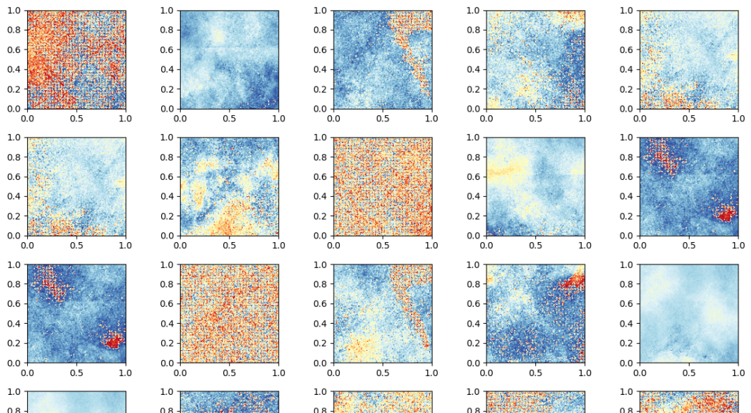
(a) Random samples from the best performing diffusion model.

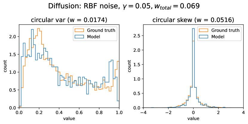
(b) Best performing diffusion model

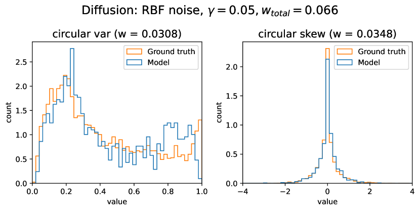
(c) Best performing GANO model

Figure 4: Results of Volcano dataset experiments (Section 5.3): Samples from the best performing FNO diffusion model with an RBF scale of $\gamma=0.05$. For both histograms, $M=1024$ generated samples were used to compute skew and variance.

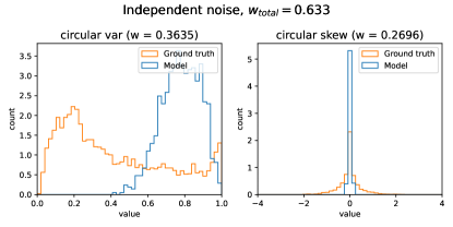
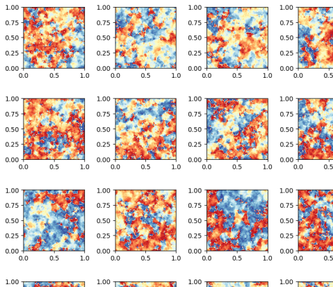
(a) Independent Gaussian noise, $w_{\text{total}}=0.633$

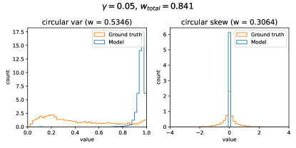
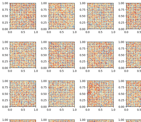
(b) RBF noise, $\gamma=0.05$, $w_{\text{total}}=0.841$

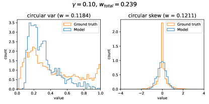
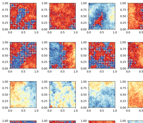
(c) RBF noise, $\gamma=0.1$, $w_{\text{total}}=0.239$

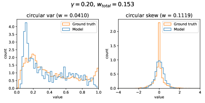
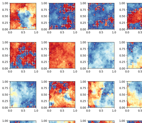
(d) RBF noise, $\gamma=0.2$, $w_{\text{total}}=0.153$

Figure 5: Super-resolution experiments for DDO. Each subplot corresponds to a different level of RBF smoothness, which is denoted by $\gamma$ (larger $\gamma$ corresponds to smoother noise). DDO is trained on $60\times 60$ resolution functions, and $120\times 120$ functions are produced as per Section 5.3. Variance and skew statistics are computed from $M=1024$ samples and the Wasserstein distance is computed between those samples and the corresponding statistics from the $120\times 120$ resolution version of the training set (i.e. the original resolution). We can see that both the independent noise experiment and $\gamma=0.05$ experiment fail to produce plausible examples.

Results

In Figure 4 we demonstrate samples and histograms produced by our best performing diffusion model, with smoothness parameter $\lambda=0.05$. These are shown in Figures 4(a) and 4(b) respectively, and a reference GANO model is also shown in 4(c). We can see that our model is able to accurately learn the ground truth function, as indicated by the histograms shown in Figure 4(b). Due to the noisiness of this dataset we found that the best results were achieved with an RBF scale parameter of $\gamma=0.05$ (see Section J.3), which corresponds to very rough levels of noise.

At generation time, in order to generate at twice the resolution we construct a meshgrid that is twice as granular as that used in training. For example, if $s^{2}$ is the original resolution then we compute a meshgrid $x\in[0,1]^{(s^{2})^{2}\times 2}$ and use that to sample RBF noise at twice the resolution. Concretely, we train DDO on a downsampled version of Volcano at $60\times 60$ resolution and double the resolution at generation time to $120\times 120$. In order to quantitatively evaluate this task we still compute skew and variance metrics as previously described (Equation 24), but now these are computed between the super-resolution samples and the original $120\times 120$ resolution dataset. These results are shown in Figure 5, and we demonstrate results comparing independent Gaussian noise to different values of RBF smoothness $\gamma$ used during training. As expected, independent noise performs abysmally (Figure 5(a)), and we also found that $\gamma=0.05$ did not perform well (Figure 5(b)). However, smoother levels of RBF noise performed well, and the best results were achieved with $\gamma=0.2$ (Figure 5(d)). This demonstrates the ability of our model to query the sampled function.

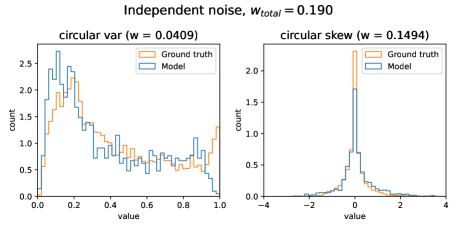
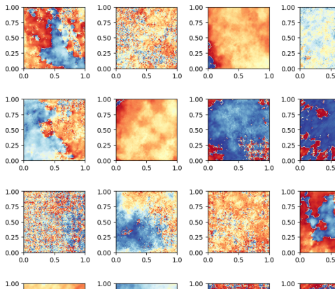
(a) Independent Gaussian noise, $w_{\text{total}}=0.187$

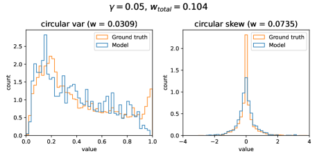
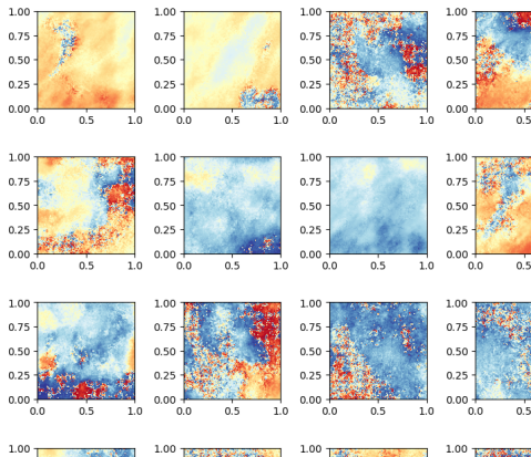
(b) RBF noise, $\lambda=0.05$, $w_{\text{total}}=0.104$

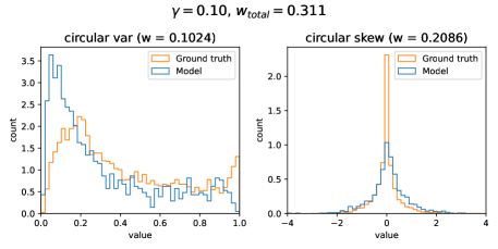
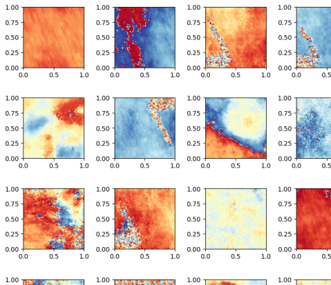
(c) RBF noise, $\lambda=0.1$, $w_{\text{total}}=0.311$

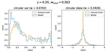
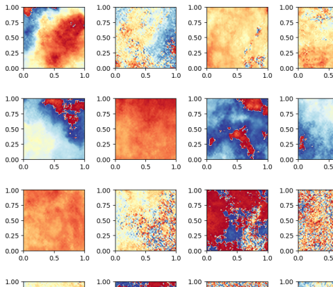
(d) RBF noise, $\lambda=0.2$, $w_{\text{total}}=0.263$

Figure 6: Super-resolution experiments for GANO. Each subplot corresponds to a different level of RBF smoothness, which is denoted by $\gamma$ (larger $\gamma$ corresponds to smoother noise). GANO is trained on $60\times 60$ resolution functions, and $120\times 120$ resolution functions are produced as per Section 5.3. Variance and skew statistics are computed from $M=1024$ samples and the Wasserstein distance is computed between those samples and the corresponding statistics from the $120\times 120$ resolution version of the training set (i.e. the original resolution).

5.4 MNIST-SDF Dataset

Finally, to demonstrate efficacy of the proposed method on function generation in conjunction with images, we conduct experiments on MNIST-SDF (Sitzmann et al., 2020) and compare the proposed method to GANO (Rahman et al., 2022), which is an adversarial training-based function space generative model. Rather than resizing finite-dimensional datasets for various resolutions, we select MNIST-SDF. MNIST-SDF is a collection of 2D SDFs, each of which is extracted by applying a distance transform to every image in the MNIST dataset. Its simplicity makes it an ideal choice, and since the dataset is defined on the function space, we can consistently compute evaluation statistics like FID (Heusel et al., 2017) and precision-recall (Kynkäänniemi et al., 2019) metrics across different resolutions. The example 2D SDFs are shown in Figure 7.(a).

We train models on 32$\times$32-resolution observation and evaluate the FID and precision-recall at different resolutions. As we find that the classifiers pre-trained for the evaluation metrics are more suitable for the original MNIST-like binary digits than 2D SDFs, we evaluate the metrics after generating binary masks by thresholding the sample SDFs to larger than $0$. The masked 2D SDFs images are illustrated in Figure 7.(b). We follow the styleGAN3’s evaluation protocol (Karras et al., 2021) for the FID and precision-recall.

However, specifically for image datasets, we choose to upsample 32$\times$32 resolution to 64$\times$64, since the number of Fourier modes to represent the data or noise is higher than the discretization. We will discuss the necessity of the upsampling in the following section, and the other experimental details, including architecture and training details, are described in the Appendix J.4

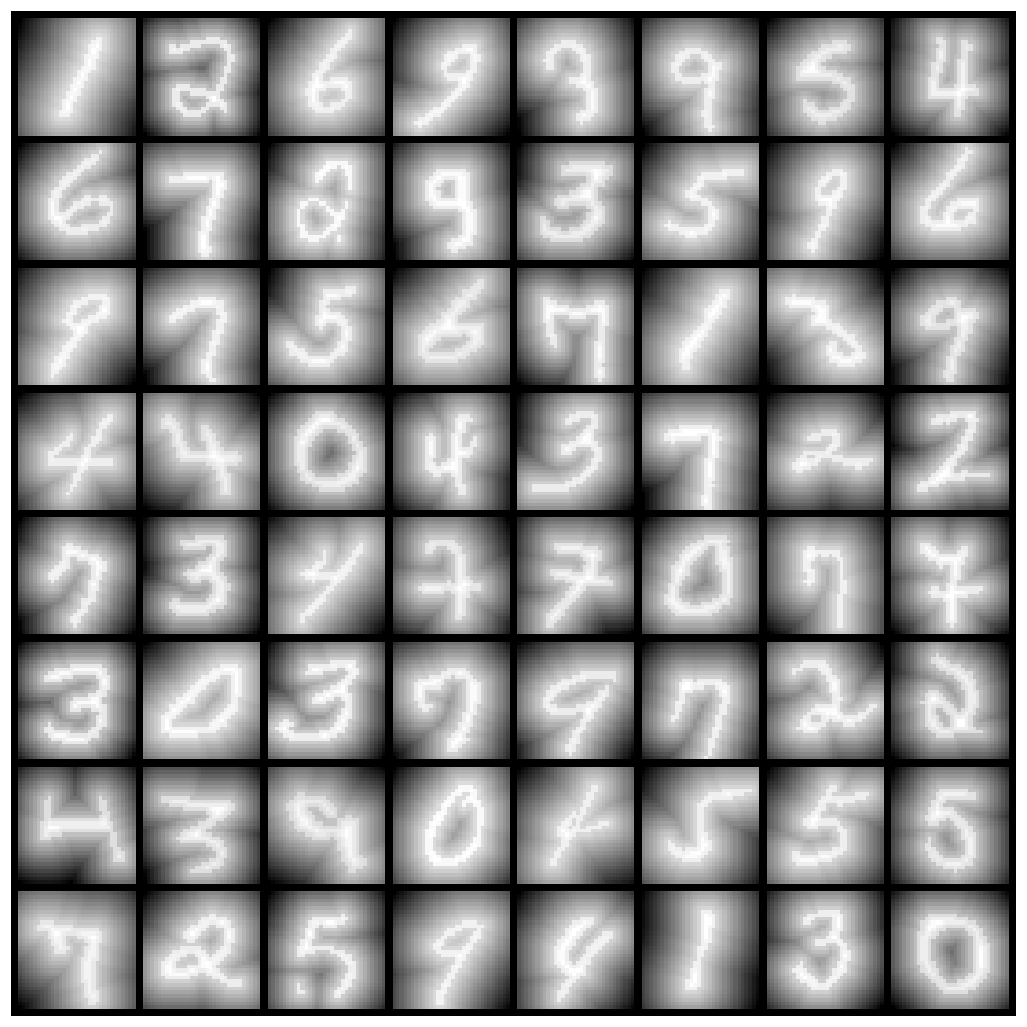
(a) MNIST-SDF

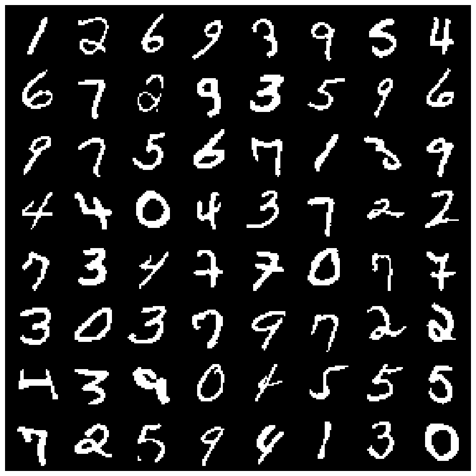
(b) Masked

Figure 7: MNIST-SDF Dataset. (a) Samples of 2D SDFs in the datasets. A 2D SDF is generated by applying a distance transform to each image in the MNIST dataset. (b) Binary masks extracted by thresholding the sample SDFs where the value is larger than $0$. Every generated samples from the models will be masked before running FID and precision-recall metrics.

Upsampling the Finite-dimensional Observations

Our theory suggests that any sample function in the target data distribution should be smoother than the samples of the noise distribution to satisfy $\mu(H_{\mu_{0}})=1$. This assumption implies that when we represent the data and noise in Fourier space, the Fourier bases required to describe all noise samples include the basis set of the data. This requirement leaves us some implementation constraints when dealing with the finite observations of the data or noises, especially when the number of bases representing a noise sample is larger than the discretization size. This is often the case since useful distributions like Gaussian measures are often obtained in $d$-dimensional observations while its basis set size is much larger than $d$. In this section, we will discuss how to address the constraints efficiently.

For most experimental scenarios, we assume that we can only access $d$-dimensional observations of the data. This means that we can treat the size of the data’s basis set to be $d$. While the true size could be larger than $d$, we won’t be able to model anything other than observations on the $d$ basis. However, we can learn such discrete observations on the Fourier bases by discrete Fourier transforms and generate arbitrary discretization from them.

On the contrary to data, for some useful distributions in the infinite-dimensional space, the size of basis sets is often larger than the observation size $d$; for example, Gaussian measures. For Gaussian, there exists a positive integer $M<\infty$ such that the $M$-size of the basis set can represent all its samples. When we select $M$ to be higher than $d$ to model the $d$-dimensional data, the components on $M$-$d$ number of bases won’t be observed at the given discretization. Thus, any model may fail to generate proper images at any resolution larger than $d$, as the unseen noise components will be introduced.

To address this, for a given $d$-dimensional observations, we propose upsampling to $d^{\prime}$ such that $d^{\prime}$ is large enough to $M$. For the 32$\times$32-resolution observation of the MNIST-SDF, we choose $d^{\prime}$ to 64$\times$64. For the upsampling of the finite observations, this paper follows the filtered upsampling implementation discussed in Karras et al. (2021). While the models are trained on 64$\times$64-resolution, we use only 32 modes to the spectral convolutions (at the lowest level) of the architectures used in DDO and GANO.

Note that one can truncate the modes of Gaussians up to $d$ so that the unseen noise components won’t be introduced. However, we find that such truncations often generate artifacts in super-resolution tasks; periodic waves are drawn, which are supposed to be straight lines.

	$64\times 64$			$128\times 128$			$256\times 256$
	FID	Prec∗	Rec†	FID	Prec	Rec	FID	Prec	Rec
GANO	3.41	0.75	0.63	13.05	0.68	0.50	23.89	0.60	0.32
DDO (Ours)	3.36	0.72	0.67	11.30	0.68	0.57	21.90	0.62	0.35
∗Precision. †Recall.

Table 1: Results of MNIST-SDF experiments.

()

()

()

()

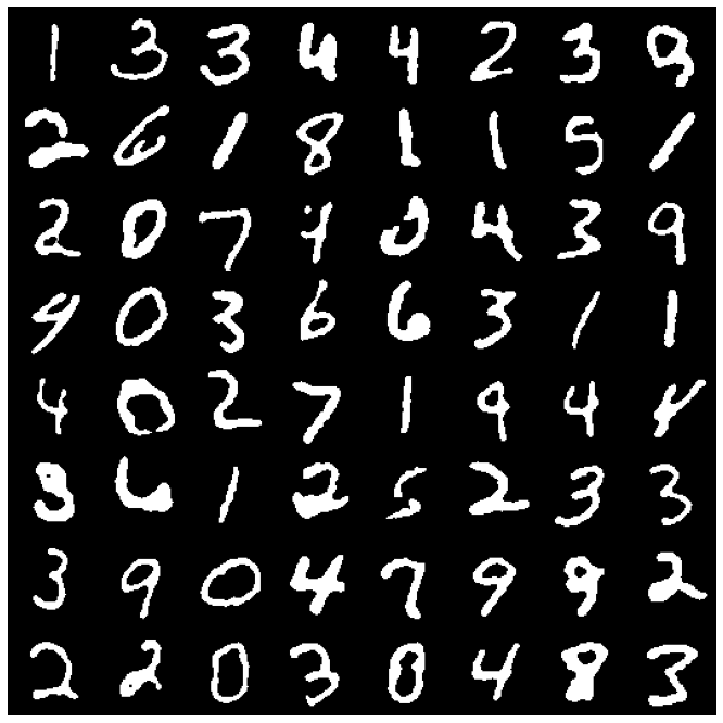
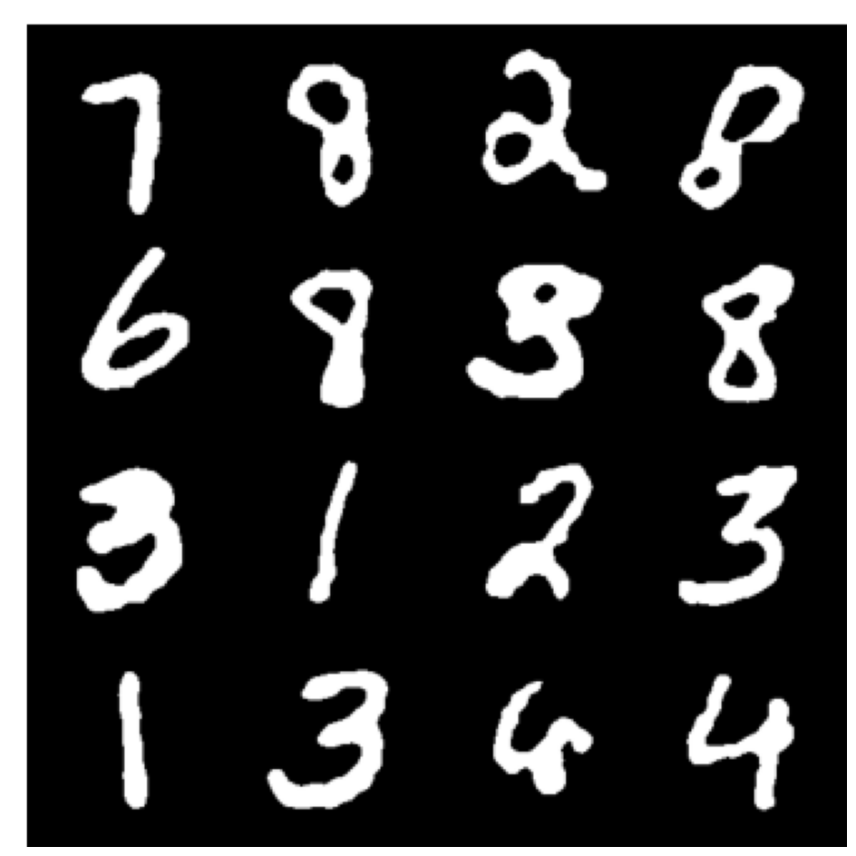
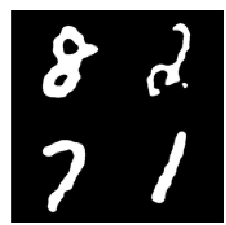
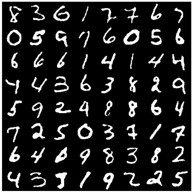
(a)  $64\times 64$

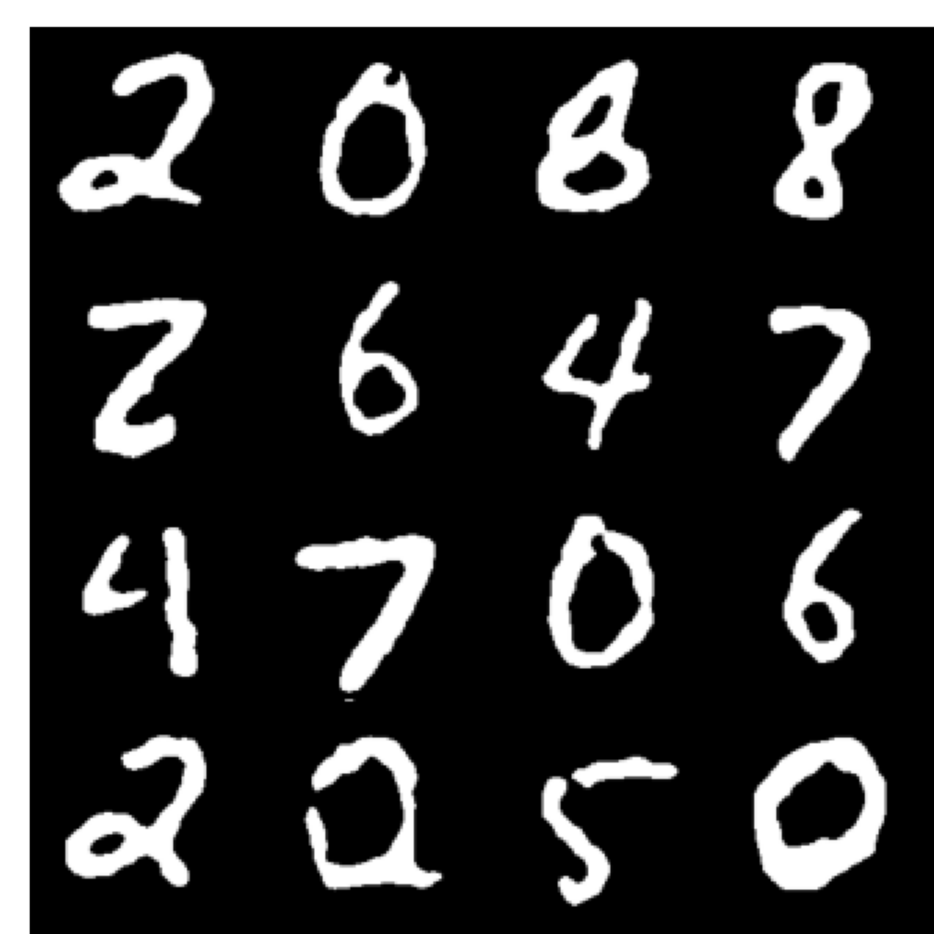
(b)  $128\times 128$

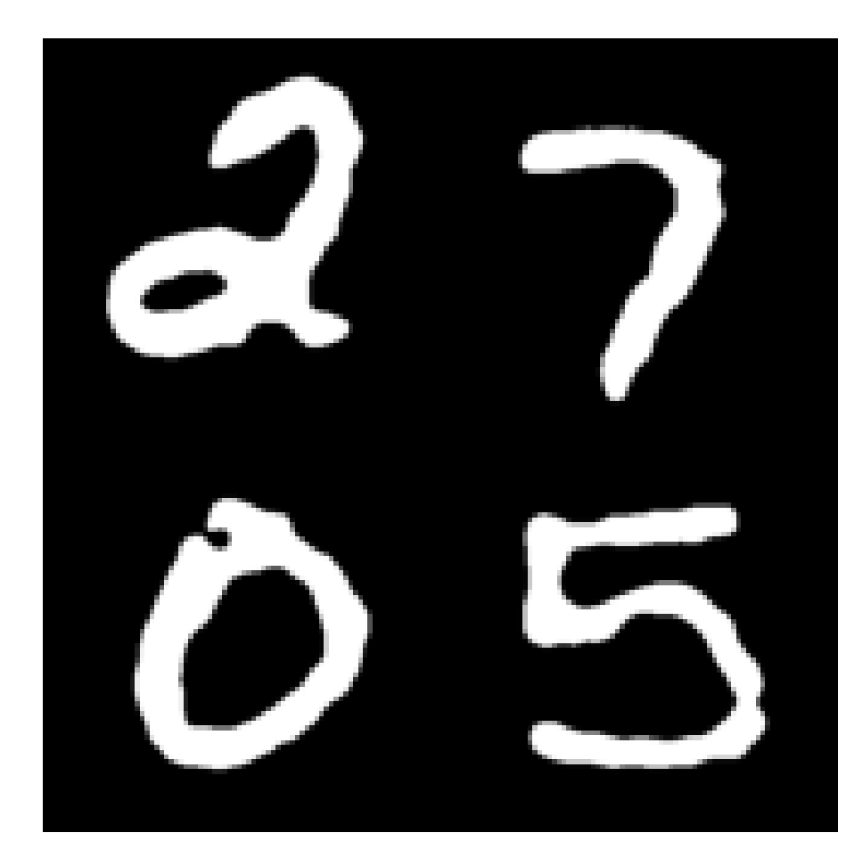
(c)  $256\times 256$

()

Figure 8: Generated Samples (Section 5.4): Generated samples (masked) of the learned GANO and DDO models at various resolutions; (a) 64$\times$64, (b) 128$\times$128, and 256$\times$256-resolutions. Both models are trained on 64$\times$64-resolution images, which are upsampled from 32$\times$32-resolution observations of 2D SDFs.

Results

Table 1 shows the FID and precision-recall metrics evaluated from learned models in the MNIST-SDF experiments. DDO outperforms the GANO baseline except for the precision at the training resolution (64$\times$64). Moreover, DDO demonstrates higher recall at all resolutions, coherent with the general property of diffusion-based models, whose objectives are to minimize KL divergence between the data distribution and the model. Note that such connections to the DDO’s objective are briefly discussed via Lemma 9.

Figure 8 illustrates the generated samples at various resolutions produced by our DDO model and the GANO baseline. Both models learn the data distribution and generate all digits at all resolutions. However, generated samples from all models show curved boundaries, which the MNIST-SDF dataset doesn’t have. This artifact originates from the spectral convolution, as it cut off higher frequency components than its parameters’ highest mode. Again, this results in the loss of some high-frequency components which would be necessary to represent arbitrary curved lines with no artifacts. This observation also emphasizes the importance of upsampling during training instead of truncating the noise. We leave addressing such artifacts for future works.

6 Discussion and Conclusions

We propose DDOs, the first theoretical framework and numerical demonstration of resolution invariant diffusion generative models on function space. Our approach generalizes denoising score matching for trace-class noise corruptions that live in the Hilbert space of the data, and considers a discrete-time diffusion model for sampling using infinite-dimensional Langevin dynamics. Future work will connect this framework with noise scales that depend continuously on time (as in Appendix C) to the forward and backward SDEs in Song et al. (2020b). Defining the backward SDE will require satisfying conditions that guarantee time reversibility of infinite-dimensional diffusions; see Föllmer and Wakolbinger (1986) for examples of these conditions. Adapting the covariance of the reference noise process based on the data distribution may also be helpful for generative modeling with other functional datasets, and to extend this framework to solve inverse problems with infinite-dimensional parameters Stuart (2010). Lastly, rigorous error analysis (e.g. using an approximate score) will be important to understand the class of data distributions that can be accurately characterized with infinite-dimensional diffusion models.

Appendix A Notation

We denote by $\mathbb{{R}}$ the real numbers and by $\mathbb{{R}}^{n}$ their $n$-fold Cartesian product and write $\|\cdot\|_{2}$ for Euclidean norm. We write $\mathbb{{N}}$ for the set of natural numbers. We denote by $H$ a real, separable, Hilbert space and by $\langle\cdot,\cdot\rangle$, $\|\cdot\|$ its inner-product and norm respectively. We write $\mathcal{B}(H)$ for the Borel sets of $H$ generated by the open sets induced from the norm topology. For probability measures $\mu,\nu$ on $\big{(}H,\mathcal{B}(H)\big{)}$, we say $\mu$ is absolutely continuous with respect to $\nu$ and denote it $\mu\ll\nu$ if, for any $B\in\mathcal{B}(H)$, $\nu(B)=0$ implies $\mu(B)=0$. If $\mu\ll\nu$ and $\nu\ll\mu$ hold then we $\mu$ and $\nu$ are equivalent and denote it $\mu\sim\nu$. If neither $\mu\ll\nu$ or $\nu\ll\mu$ hold then we say $\mu$ and $\nu$ are mutually singular and denote it $\mu\perp\nu$. We say $u$ is a random variable distributed according to $\mu$ and denote it $u\sim\mu$ if the law of $u$ is $\mu$. Given two random variables $u,v$, we write $u\perp v$ if they are independent. For any mapping, $f:H\to\mathbb{{R}}$, we denote by $\mathbb{{E}}_{u\sim\mu}[f(u)]$ the expected value of $f$ under $\mu$.

For any bounded operator $C:H\to H$, we say $C$ is self-adjoint if $\langle Cu,v\rangle=\langle u,Cv\rangle$ for all $u,v\in H$. We say an operator is positive if $\langle Cu,u\rangle>0$ for all $u\in H\setminus\{0\}$ (equivalently non-negative if $\langle Cu,u\rangle\geq 0$). We say $C$ is trace-class, or nuclear, if for any orthonormal basis $\{\phi_{j}\}_{j=1}^{\infty}$ of $H$, we have $\text{Tr}(C)=\sum_{j=1}^{\infty}\langle C\phi_{j},\phi_{j}\rangle<\infty$. For any self-adjoint, non-negative, trace-class operator, we denote by $C^{1/2}$ the unique operator such that $C=C^{1/2}C^{1/2}$. We denote by $H^{*}$ the topological (continuous) dual $H$ which is itself a separable Hilbert space consisting of all bounded linear functionals $l:H\to\mathbb{{R}}$ with an inner-product induced by the Reisz map. Since it follows by the Riesz representation theorem that for any $l\in H^{*}$, there exists a unique element $v\in H$ such that $l(u)=\langle u,v\rangle$ for any $u\in H$, we define the Riesz map $R:H^{*}\to H$ by $l\mapsto v$.

Table 2: Score-based diffusion models: from finite to infinite dimension.

Setting	Finite dimension	Infinite dimension
Data space	Euclidean spaces	Function spaces
Base measures	Lebesgue measure	Gaussian random fields
Noise in diffusion	Multivariate random variables	Gaussian random fields
Score	Score function	Score operator
Process	Langevin process in finite dimensions $y$	Langevin process in function spaces
Learning loss	Euclidean norm	Norm on function spaces
		(discretization invariant)
Controls	Variance	Length scale, variance, energy, etc.
Base model	Neural networks	Neural operators

Appendix B Proofs of Theorem

B.1 Convolution of measures

The following results holds more generally for Radon Gaussian measures on locally convex spaces. We show them here in the Hilbert space setting to avoid introducing extra notation but refer the reader to Bogachev (2015) for a thorough overview of the more general setting.

Let $(H,\langle\cdot,\cdot\rangle)$ be a real, separable, Hilbert space and $\mu$ and $\nu$ be two probability measures on the Borel $\sigma$-algebra $\mathcal{B}(H)$. Then the product measure $\mu\otimes\nu$ is defined on $\mathcal{B}(H)\otimes\mathcal{B}(H)=\mathcal{B}(H\times H)$. Define the mapping $T:H\times H\to H$ by $T(u,v)=u+v$. Then the pushforward of $\mu\otimes\nu$ under $T$ is called the convolution of $\mu$ and $\nu$ and is denoted $\mu*\nu$. In particular, given two independent random variables $u\sim\mu$ and $v\sim\nu$, the random variable $u+v$ is distributed according to $\mu*\nu$. It can be shown that, for any $B\in\mathcal{B}(H)$, we have

$$(\mu*\nu)(B)=\int_{H}\mu(B-v)\>d\nu(v)=\int_{H}\nu(B-u)\>d\mu(u)=(\nu*\mu)(B),$$ (27)

for example, see Appendix A.3 in Bogachev (2015) and references therein. The following result shows that if $\nu$ is a centered Gaussian and $\mu$ charges its Cameron-Martin space, the convolution is equivalent, in the sense of measures, to $\nu$.

Theorem 5

Let $\mu,\nu$ be two probability measures on $(H,\mathcal{B}(H))$ with $\nu=N(0,C)$ for some $C:H\to H$ self-adjoint, positive, and trace-class. If $\mu(C^{1/2}(H))=1$, then $\nu_{u}\sim\nu$ where $\nu_{u}$ is the conditional for $v|u$ and $\nu*\mu\sim\nu$.

Proof  For any $B\in\mathcal{B}(H)$, we have by (27),

$$(\nu*\mu)(B)=\int_{H}\nu(B-u)\>d\mu(u).$$

Therefore $(\nu*\mu)(B)=0$ if and only if $\nu(B-u)=0$ for $\mu$-almost any $u\in H$ since $\nu$ is non-negative. For any $u\in H$, define the measures

$$\nu_{u}(B)=\nu(B-u),\qquad\forall B\in\mathcal{B}(H)$$

which are Gaussian $\nu_{u}=N(u,C)$. By the Cameron-Martin Theorem, given as Proposition 2.26 in Da Prato et al. (1992), $\nu_{u}\ll\nu$ for any $u\in C^{1/2}(H)$. Let $B\in\mathcal{B}(H)$ be such that $\nu(B)=0$. Since, $\nu_{u}\ll\nu$ for any $u\in C^{1/2}(H)$, we have that $\nu(B-u)=0$. Since $\mu(C^{1/2}(H))=1$, $\nu(B-u)=0$ for $\mu$-almost any $u\in H$ and therefore $\nu*\mu\ll\nu$.

Now let $B\in\mathcal{B}(H)$ be such that $(\nu*\mu)(B)=0$ then $\nu_{u}(B)=0$ for $\mu$-almost any $u\in H$. Since $\mu(C^{1/2}(H))=1$, again by the Cameron-Martin Theorem, $\nu_{u}\ll\nu$. But, by Theorem 2.25 in Da Prato et al. (1992), Gaussians are either equivalent or mutually singular , therefore $\nu\ll\nu_{u}$ and thus $\nu(B)=0$ hence the result follows.  

Let $A:H\to H$ be a linear operator. If $u\sim\mu$, then from definition, the random variable $Au$ is distributed according to the measure $\mu\circ A^{-1}$ where $A^{-1}$ denotes the pre-image of $A$. In particular, for any $B\in\mathcal{B}(H)$,

$$(\mu\circ A^{-1})(B)=\mu(\{u\in H:Au\in B\}).$$ (28)

The following corollary of Theorem 5 addresses random variables of the form $Au+v$ where $u\sim\mu$ and $v\sim\nu$ are independent.

Corollary 6

Let $\mu,\nu$ be two probability measures on $(H,\mathcal{B}(H))$ with $\nu=N(0,C)$ for some $C:H\to H$ self-adjoint, positive, and trace-class. Let $A:H\to H$ be a linear operator such that $A(H)\subseteq C^{1/2}(H)$ then $\nu*(\mu\circ A^{-1})\sim\nu$.

Proof  From equation (28) and the assumption that $A(H)\subseteq C^{1/2}(H)$, we have

$$(\mu\circ A^{-1})\big{(}C^{1/2}(H)\big{)} =\mu\big{(}\{u\in H:Au\in C^{1/2}(H)\}\big{)}$$

$$=\mu(H)$$

$$=1.$$

Thus the result follows by Theorem 5.  

B.2 Conditional scores

Let $H$ be a real, separable, Hilbert space and denote by $\mathcal{B}(H)$ its Borel $\sigma$-algebra. Let $\gamma$ be a probability measure on $\big{(}H\times H,\mathcal{B}(H)\otimes\mathcal{B}(H)\big{)}$. We introduce the coordinates $(u,v)\sim\gamma$. Denote by $\mu$ marginal of $u$, by $\nu$ the marginal of $v$, and by $\gamma^{u}$ the conditional $v|u$ for $\mu$-almost any $u\in H$. Let $\mu_{0}$ be a probability measure on $\big{(}H,\mathcal{B}(H)\big{)}$ and suppose that $\nu\ll\mu_{0}$ and $\gamma^{u}\ll\mu_{0}$ for $\mu$-almost any $u\in H$.

Lemma 7

The Radon–Nikodym derivatives of $\nu$ and $\gamma^{u}$ with respect to $\mu_{0}$ satisfy

$$\frac{d\nu}{d\mu_{0}}(v)=\mathbb{{E}}_{u\sim\mu}\frac{d\gamma^{u}}{d\mu_{0}}(v),\qquad\text{for }\mu_{0}\text{-almost any }v\in H.$$

Proof  Let $B\in\mathcal{B}(H)$ then by definition of a conditional measure and Fubini’s Theorem,

$$\nu(B) =\int_{H}\int_{B}d\gamma^{u}(v)d\mu(u)$$

$$=\int_{H}\int_{B}\frac{d\gamma^{u}}{d\mu_{0}}(v)d\mu_{0}(v)d\mu(u)$$

$$=\int_{B}\left(\int_{H}\frac{d\gamma^{u}}{d\mu_{0}}(v)d\mu(u)\right)d\mu_{0}(v).$$

We also have,

$$\nu(B)=\int_{B}\frac{d\nu}{d\mu_{0}}(v)d\mu_{0}(v).$$

Therefore

$$\int_{B}\frac{d\nu}{d\mu_{0}}(v)d\mu_{0}(v)=\int_{B}\left(\int_{H}\frac{d\gamma^{u}}{d\mu_{0}}(v)d\mu(u)\right)d\mu_{0}(v).$$

Since $B$ is arbitrary, we must have that

$$\frac{d\nu}{d\mu_{0}}(v)=\int_{H}\frac{d\gamma^{u}}{d\mu_{0}}(v)d\mu(u)$$

for $\mu_{0}$-almost any $v\in H$ which is the desired result.  

Let $E\subseteq H$ be a Hilbert space continuously embedded in $H$ and denote by $D_{E}$ the Frechet differential operator on $H$ in the direction of $E$. Suppose that $\nu\sim\mu_{0}$ and $\gamma^{u}\sim\mu_{0}$ so that all respective Radon–Nikodym derivatives exist and are positive. Define,

$$\Phi(v)\coloneqq\log\frac{d\nu}{d\mu_{0}}(v),\quad\Psi(v;u)\coloneqq\log\frac{d\gamma^{u}}{d\mu_{0}}(v)$$

for $\mu_{0}$-almost ant $v\in H$ and $\mu$-almost any $u\in H$. Suppose that $\Phi$ and $\Psi(\cdot;u)$ are once $D_{E}$-continuously differentiable . Furthermore assume

$$\mathbb{{E}}_{v\sim\nu}\|D_{E}\Phi(v)\|_{E^{*}}^{2}<\infty,\quad\mathbb{{E}}_{u\sim\mu}\mathbb{{E}}_{v\sim\gamma^{u}}\|D_{E}\Psi(v;u)\|_{E^{*}}^{2}<\infty$$

where $E^{*}$ denotes the topological dual of $E$. Let $G_{\theta}:H\to E^{*}$ be a parametric mapping with parameters $\theta\in\mathbb{R}^{p}$. Assume that, for all $\theta\in\mathbb{R}^{p}$,

$$\mathbb{{E}}_{v\sim\nu}\|G_{\theta}(v)\|_{E^{*}}^{2}<\infty.$$

Define the functionals,

$$F(\theta) \coloneqq\mathbb{{E}}_{v\sim\nu}\|D_{E}\Phi(v)-G_{\theta}(v)\|^{2}_{E^{*}}$$

$$J(\theta) \coloneqq\mathbb{{E}}_{u\sim\mu}\mathbb{{E}}_{v\sim\gamma^{u}}\|D_{E}\Psi(v;u)-G_{\theta}(v)\|_{E^{*}}^{2}.$$

Theorem 8

There exists a constant $C<\infty$ independent of $\theta\in\mathbb{R}^{p}$ such that

$$F(\theta)=J(\theta)+C,\qquad\forall\>\theta\in\mathbb{R}^{p}.$$

Proof  We have

$$F(\theta)=\mathbb{{E}}_{v\sim\nu}\left[\|G_{\theta}(v)\|_{E^{*}}^{2}-2\langle D_{E}\Phi(v),G_{\theta}(v)\rangle_{E^{*}}\right]+C_{1}$$

where $C_{1}=\mathbb{{E}}_{v\sim\nu}\|D_{E}\Phi(v)\|_{E^{*}}^{2}<\infty$ by assumption. Similarly,

$$J(\theta)=\mathbb{{E}}_{u\sim\mu}\mathbb{{E}}_{v\sim\gamma^{u}}\left[\|G_{\theta}(v)\|_{E^{*}}^{2}-2\langle D_{E}\Psi(v;u),G_{\theta}(v)\rangle_{E^{*}}\right]+C_{2}$$

where $C_{2}=\mathbb{{E}}_{u\sim\mu}\mathbb{{E}}_{v\sim\gamma^{u}}\|D_{E}\Psi(v;u)\|_{E^{*}}^{2}<\infty$ by assumption. By definition of a conditional measure,

$$\mathbb{{E}}_{v\sim\nu}\|G_{\theta}(v)\|_{E^{*}}^{2}=\mathbb{{E}}_{u\sim\mu}\mathbb{{E}}_{v\sim\gamma^{u}}\|G_{\theta}(v)\|_{E^{*}}^{2}$$

for any $\theta\in\mathbb{R}^{p}$. Using Lemma 7, the Leibniz integral rule, and Fubini’s Theorem, we find

$$\mathbb{{E}}_{v\sim\nu}\langle D_{E}\Phi(v),G_{\theta}(v)\rangle_{E^{*}} =\mathbb{{E}}_{v\sim\nu}\langle D_{E}\log\frac{d\nu}{d\mu_{0}}(v),G_{\theta}(v)\rangle_{E^{*}}$$

$$=\mathbb{{E}}_{v\sim\nu}\langle\frac{d\mu_{0}}{d\nu}(v)D_{E}\frac{d\nu}{d\mu_{0}}(v),G_{\theta}(v)\rangle_{E^{*}}$$

$$=\mathbb{{E}}_{v\sim\mu_{0}}\langle D_{E}\frac{d\nu}{d\mu_{0}}(v),G_{\theta}(v)\rangle_{E^{*}}$$

$$=\mathbb{{E}}_{v\sim\mu_{0}}\langle D_{E}\mathbb{{E}}_{u\sim\mu}\frac{d\gamma^{u}}{d\mu_{0}}(v),G_{\theta}(v)\rangle_{E^{*}}$$

$$=\mathbb{{E}}_{v\sim\mu_{0}}\langle\mathbb{{E}}_{u\sim\mu}D_{E}\frac{d\gamma^{u}}{d\mu_{0}}(v),G_{\theta}(v)\rangle_{E^{*}}$$

$$=\mathbb{{E}}_{v\sim\mu_{0}}\langle\mathbb{{E}}_{u\sim\mu}\frac{d\gamma^{u}}{d\mu_{0}}(v)D_{E}\log\frac{d\gamma^{u}}{d\mu_{0}}(v),G_{\theta}(v)\rangle_{E^{*}}$$

$$=\mathbb{{E}}_{v\sim\mu_{0}}\mathbb{{E}}_{u\sim\mu}\frac{d\gamma^{u}}{d\mu_{0}}(v)\langle D_{E}\log\frac{d\gamma^{u}}{d\mu_{0}}(v),G_{\theta}(v)\rangle_{E^{*}}$$

$$=\mathbb{{E}}_{u\sim\mu}\mathbb{{E}}_{v\sim\mu_{0}}\frac{d\gamma^{u}}{d\mu_{0}}(v)\langle D_{E}\Psi(v;u),G_{\theta}(v)\rangle_{E^{*}}$$

$$=\mathbb{{E}}_{u\sim\mu}\mathbb{{E}}_{v\sim\gamma^{u}}\langle D_{E}\Psi(v;u),G_{\theta}(v)\rangle_{E^{*}}.$$

Setting $C=C_{1}-C_{2}$ completes the proof.  

It remains to show that approximating the score of the convolved measure ensues we are close to the true measures. The following lemma relates the Wasserstein distance of the two.

Lemma 9

Let $\eta\sim\mu_{\sigma}$ be a noise random variable with finite $p$-moment, and let $v=u+\eta\sim\mu*\mu_{\sigma}$. Then, the Wasserstein-p distance for $p\geq 1$ satisfies $W_{p}(\mu*\mu_{\sigma},\mu)\leq\|\eta\|_{L^{p}(\mu_{\sigma})}$.

Proof  Let $(u,\eta)$ follow the product coupling $(\mu\otimes\mu_{\sigma})(du,d\eta)$. Then, let the coupling $(v,\eta)$ where $v=u+\eta$ be drawn according to $(u+\eta,u)_{\sharp}(\mu\otimes\mu_{\sigma})(du,d\eta)$. Choosing this coupling $(v,\eta)$ to upper bound the Wasserstein-p distance, we have

$$W_{p}(\mu*\mu_{\sigma},\mu)^{p}=\inf_{\gamma\in\Pi(\mu*\mu_{\sigma},\mu)}\int|v-u|^{p}d\gamma(v,u)\leq\int|(u+\eta)-u|^{p}(\mu\otimes\mu_{\sigma})(du,d\eta).$$

Given that the integrand is independent of $u$, we have $W_{p}(\mu*\mu_{\sigma},\mu)^{p}\leq\int|\eta|^{p}d\mu_{\sigma}=\|\eta\|_{L^{p}(\mu_{\sigma})}^{p}$, and the result follows.  

Remark 10

For a Gaussian measure $\mu_{\sigma}$, the $p$-th moment is finite by the Fernique Theorem. Moreover, by Theorem 6.6 in Stuart (2010) there is a constant $C_{p}>0$ so that $\|\eta\|_{L^{p}}\leq C_{p}(\text{Tr}(C_{\sigma}))$. This can be used to establish the convergence rate of $W_{p}(\mu*\mu_{\sigma},\mu)\rightarrow 0$ as $\sigma\rightarrow 0$.

Lemma 11

The Fréchet derivative $D_{H_{\mu_{0}}}\Psi(w;u)$ as defined in (10) is in $H_{\mu_{0}}^{*}$.

Proof  Notice that since $u\in H_{\mu_{0}}$, $\mu$-almost surely, we can find $g\in H$ such that $u=C^{1/2}g$. For any $w\in H_{\mu_{0}}$, we can similarly find $f\in H$ such that $w=C^{1/2}f$. We can write both $g$ and $f$ in the othronormal basis $\{\varphi_{j}\}_{j=1}^{\infty}$,

$$g=\sum_{j=1}^{\infty}\langle g,\varphi_{j}\rangle\varphi_{j},\qquad f=\sum_{j=1}^{\infty}\langle f,\varphi_{j}\rangle\varphi_{j}$$

with both series converging in $H$. Orthonormality implies

$$\langle u,\varphi_{j}\rangle=\lambda_{j}^{1/2}\langle g,\varphi_{j}\rangle,\qquad\langle w,\varphi_{j}\rangle=\lambda_{j}^{1/2}\langle f,\varphi_{j}\rangle$$

for any $j\in\mathbb{N}$. Therefore equation (11) becomes

$$D_{H_{\mu_{0}}}\Psi(v;u)w =\sum_{j=1}^{\infty}\langle g,\varphi_{j}\rangle\langle f,\varphi_{j}\rangle$$

$$\leq\left(\sum_{j=1}^{\infty}|\langle g,\varphi_{j}\rangle|^{2}\right)^{1/2}\left(\sum_{j=1}^{\infty}|\langle f,\varphi_{j}\rangle|^{2}\right)^{1/2}$$

$$=\|g\|\|f\|$$

which is finite hence the result follows.  

Appendix C Multiple Noise Scales

To satisfy our absolute continuity condition for the perturbed data measure in Sections 4.3 and 4.4, we need $A_{t}(H)\subseteq\text{Im}(C_{t}^{1/2})$ for all $t$. The following lemmas show that this condition holds for different time-dependent scalar weightings of the forward and noise covariance operators.

Lemma 12

Let $\eta_{t}\sim\mu_{t}=\mathcal{N}(0,C_{t})$ where $C_{t}=g(t)C$ and $v_{t}=A_{t}u+\eta_{t}$ where $A_{t}=f(t)u$ for all $t\in I$ for $u\in H$. Assuming the mappings $f,g:\mathcal{{I}}\to\mathbb{{R}}$ satisfy $0<M_{1}\leq f(t),g(t)\leq M_{2}$ for all $t\in\mathcal{{I}}$ and $\mu\big{(}C^{1/2}(H)\big{)}=1$, then $A_{t}(H)\subseteq C_{t}^{1/2}(H)$ for all $t\in\mathcal{{I}}$

Proof  Let $L_{t}=g(t)/f(t)C$. We will first show that $L_{t}^{1/2}(H)=C^{1/2}(H)$. By Lemma 6.15 in Stuart (2010), the image of the two positive-definite, and self-adjoint linear operators on a Hilbert space $H$ are equal if and only if there exists constants $K_{1},K_{2}>0$ such that $K_{1}\langle u,Cu\rangle\leq\langle u,L_{t}u\rangle\leq K_{2}\langle u,Cu\rangle$ for all $u\in H$.

Under the conditions on $f,g$, for any $u\in H$, we have

$$\langle u,Cu\rangle=\langle u,\frac{f(t)g(t)}{f(t)g(t)}Cu\rangle\leq\frac{M_{2}}{M_{1}}\langle u,\frac{g(t)}{f(t)}Cu\rangle =K_{1}\langle u,L_{t}u\rangle$$

$$=K_{1}\langle u,\frac{g(t)}{f(t)}Cu\rangle\leq K_{1}\frac{M_{2}}{M_{1}}\langle u,Cu\rangle=K_{2}\langle u,Cu\rangle,$$

where $K_{1}=M_{2}/M_{1}$ and $K_{2}=K_{1}^{2}$. Then, for $\mu\big{(}C^{1/2}(H)\big{)}=1$ we have $u\in C^{1/2}(H)$ for $u\in H$. From the image equivalence, we have $u\in L_{t}^{1/2}(H)$ and so $A_{t}u=f(t)u\in C_{t}^{1/2}(H)$.  

Lemma 13

Let $C_{t}=f(t)AA^{*}$ where $A\colon H\rightarrow H$ is a linear operator and $f\colon[0,T]\rightarrow\mathbb{R}$ is a function satisfiying $c=\sup_{t\in[0,T]}1/f(t)<+\infty$. Then, for $K=AA^{*}$ we have that $\text{Im}(K^{1/2})\subseteq\text{Im}(C_{t}^{1/2})$ for all $t\in[0,T]$.

Proof  The image of $A$ is equivalent to image of the $K^{1/2}$ where $K=AA^{*}$ is a positive-definite, and self-adjoint operator. For any $u\in H$, we have

$$\langle u,Ku\rangle=\langle u,AA^{*}f(t)/f(t)u\rangle\leq\sup_{t\in[0,T]}\frac{1}{f(t)}\langle u,AA^{*}f(t)u\rangle=c\langle u,C_{t}u\rangle.$$

The result on the image spaces follows by Lemma 6.15 in Stuart (2010).  

Example 2

The function $f(t)=e^{\gamma t}$ for $\gamma>0$ satisfies the condition in the lemma above with $c=1$. This choice motivates the following study.

Alternatively, we can define the forward process for data corruption with multiple noise scales using a stochastic differential equation (SDE), as in Song et al. (2020b). Let us consider the linear SDE $du_{t}=-Lu_{t}dt+dW_{t}$ for $u_{t}\in H$ where $W_{t}$ is a $Q$-Wiener process and $L\colon H\rightarrow H$ is a linear and positive-definite operator where its eigenvectors form an orthonormal basis for $H$. The solution of this SDE for any $t>0$ is given by

$$u(t)=e^{-Lt}u(0)+\int_{0}^{t}e^{L(s-t)}dW_{s}.$$

Letting $u(0)=u$ and $A_{t}\coloneqq e^{-Lt}$, we can treat $u\mapsto A_{t}u$ as the forward model and the second term $\eta_{t}\coloneqq\int_{0}^{t}e^{L(s-t)}dW_{s}$ as the additive noise process, which is drawn independently of $u$. The following abridged theorem from Da Prato et al. (1992) describes the statistical properties of the noise process.

Theorem 14

Assuming $\int_{0}^{T}\text{Tr}[A_{r}QA_{r}^{*}]dr<\infty$, then (i) $\eta_{t}$ is Gaussian, (ii) has continuous paths, and (iii) its covariance is given by

$$C_{t}\coloneqq\text{Cov}(\eta_{t})=\int_{0}^{t}A_{r}QA^{*}_{r}dr,\quad t\in[0,T].$$

To satisfy the absolute continuity conditions on the perturbed data measure for $u(t)$ as before, we need to show that for each $t$, $A_{t}(H)\subseteq\text{Im}(C_{t}^{1/2})$. As shown in Corollary B.7 of Da Prato et al. (1992), the image of $C_{t}^{1/2}$ for a covariance of the form above is equivalent to the image of the linear operator $B_{t}\colon H\rightarrow H$ defined as

$$B_{t}u\coloneqq\int_{0}^{t}L_{t-s}Quds.$$

$B_{t}$ and $A_{t}$ are both linear and self-adjoint operators, so the condition $\text{Im}(A_{t})\subseteq\text{Im}(B_{t})$ holds if and only if there exists a constant $K>0$ so that $\langle u,A_{t}u\rangle\leq K\langle u,B_{t}u\rangle$ for all $u\in H$. Using the decomposition of $u=\sum_{j=1}^{\infty}\langle u,\psi_{j}\rangle\psi_{j}$ where $\{\psi_{j}\}_{j=1}^{\infty}$ are eigenvectors and $\{\lambda_{j}\}_{j=1}^{\infty}$ are eigenvalues of $L$, we have

$$A_{t}u=\sum_{j}e^{-Lt}\langle u,\psi_{j}\rangle\psi_{j}=\sum_{j}e^{-\lambda_{j}t}\langle u,\psi_{j}\rangle\psi_{j}.$$

Choosing the noise covariance to be $Q=L^{\gamma}$ for some scalar $\gamma$ such that draws remain in $H$, we have

$$B_{t}u =\int_{0}^{t}\sum_{j}e^{-L(t-s)}\langle u,\psi_{j}\rangle Q\psi_{j}ds$$

$$=\int_{0}^{t}\sum_{j}e^{-\lambda_{j}(t-s)}\langle u,\psi_{j}\rangle\lambda_{j}^{\gamma}\psi_{j}ds$$

$$=\sum_{j}\langle u,\psi_{j}\rangle\lambda_{j}^{\gamma}\psi_{j}\int_{0}^{t}e^{-\lambda_{j}(t-s)}ds$$

$$=\sum_{j}\langle u,\psi_{j}\rangle\lambda_{j}^{\gamma-1}(1-e^{-\lambda_{j}t})\psi_{j}.$$

We can now compare the images of the operators. For $u\in H$ we have

$$\langle u,A_{t}u\rangle=\sum_{j}e^{-2\lambda_{j}t}|\langle u,\psi_{j}\rangle|^{2},\qquad\langle u,B_{t}u\rangle=\sum_{j}\lambda_{j}^{2(\gamma-1)}(1-e^{-2\lambda_{j}t})^{2}|\langle u,\psi_{j}\rangle|^{2}.$$

For each $\lambda_{j}>0$, there exists a time $t_{j}$ such that $e^{-2\lambda_{j}t}\leq\lambda_{j}^{2(\gamma-1)}(1-e^{-2\lambda_{j}t})^{2}$ for all $t>t_{j}$. For these times, we satisfy the condition required for our theory. Generalizing these results is an important direction for future work.

Appendix D Discretization of the Langevin Equation

We will work in the setting of multiple noise scale as introduced in Section 4.4. We show two different discretization of (13) and relate them to existing methods in the literature.

D.1 Euler-Maruyama

Let $F:H\times\mathcal{{I}}\to H$ be defined as $F(u,t)=-u+RD_{H_{\mu_{t}}}\Phi(u,t)$. For a fixed $t\in\mathcal{{I}}$, we can apply to the Euler-Maruyama scheme to (13) to obtain the iteration

$$u_{n+1}=u_{n}+h_{t}F(u_{n},t)+\sqrt{2h_{t}}\eta^{(t)}_{n}$$ (29)

for any $n\in\mathbb{{N}}$ where $\eta^{(t)}_{n}\sim\mu_{t}$ form an i.i.d. sequence and $h_{t}>0$ is fixed. Fix $t_{0}\in\mathcal{{I}}$. For any $v\in H$, the iteration in (29) starting with $u_{0}=v$ at $t=t_{0}$ transforms $v$ to an approximate sample of $\nu_{t_{0}}$. We denote this by $v_{t_{0}}$. Now fix $t_{1}\in\mathcal{{I}}$. We again run the iteration (29) with $t=t_{1}$ and $u_{0}=v_{t_{0}}$. This will transform $v_{t_{0}}$ into an approximate sample from $\nu_{t_{1}}$ which we denote $v_{t_{1}}$. If $\mathcal{{I}}=\{1,\dots,T\}$ for some $T\in\mathbb{{N}}$ then repeating this process yields $v_{T}$, which is approximately distributed according to $\nu_{T}$. By choosing some sequence $0<\sigma_{T}\leq\dots\leq\sigma_{1}$ as well as $A_{t}=I$, $\mu_{t}=N(0,\sigma_{t}^{2}C)$ in (23), and $h_{t}=\epsilon\sigma_{t}^{2}/\sigma_{T}^{2}$ for some $\epsilon>0$ and self-adjoint, positive, trace-class $C$, we recover an infinite-dimensional generalization to the NCSN algorithm of Song and Ermon (2019). In particular, our sample $v_{T}$ is approximately distributed according to the measure $\nu_{T}=\mu*N(0,\sigma_{T}^{2}C)$ where $\sigma_{T}^{2}\ll 1$ is small. Thus according to Lemma 9, $v_{T}$ is approximately distributed according to our data measure $\mu$. We outline this process in Algorithm 1.

Algorithm 1 Annealed Langevin Dynamics

  Input: $F_{\theta}$, $u_{0}\in H$, $\{\sigma_{t}\}_{t=1}^{T}$, $M\in\mathbb{{N}}$, $\epsilon>0$

  for $t=1$ to $T$ do

     $h_{t}=\epsilon\sigma_{t}^{2}/\sigma_{T}^{2}$.

     for $n=0$ to $M-1$ do

        $\eta^{(t)}_{n}\sim N(0,C)$

        $u_{n+1}=u_{n}+h_{t}F_{\theta}(u_{n},t)+\sqrt{2h_{t}}\eta^{(t)}_{n}$

     end for

     $u_{0}=u_{M}$

  end for

D.2 Crank–Nicolson

With the notation of Section D.1, we apply the Crank–Nicolson method to the linear part of the drift in (13) to obtain

$$(2+h_{t})u_{n+1}=(2-h_{t})u_{n}+2h_{t}G(u_{n},t)+\sqrt{8h_{t}}\eta^{(t)}_{n}$$ (30)

where we define $G:H\times\mathcal{{I}}\to H$ by $G(u,t)=RD_{H_{\mu_{t}}}\Phi(u,t)$ and $h_{t}>0$. For any $h_{t}\in(0,2)$, (30) can be written as

$$u_{n+1}=\alpha_{t}u_{n}+(1-\alpha_{t})G(u_{n},t)+\beta_{t}\eta^{(t)}_{n}$$ (31)

with the transformation $\beta_{t}^{2}=8h_{t}/(2+h_{t})^{2}$ where $\beta_{t}\in(0,1)$ and we define $\alpha_{t}=\sqrt{1-\beta_{t}^{2}}$. Equation (31) is a type of Metropolis-adjusted Langevin proposal in the function space setting and is related to the celebrated pre-conditioned Crank–Nicolson MCMC method Cotter et al. (2013). We remark that the iteration (31) resembles the exact, single-step, Gaussian approximation sampling method of Ho et al. (2020). We leave for future work designing and analyzing algorithms based on this approach.

Appendix E Denoising Diffusion Probabilistic Models

In Section 4.4 we showed that for a particular choice of data and noise scaling, we may recover the forward process of the DDPM framework proposed in Ho et al. (2020). Let us recall the noise process in DDPM: for some sequence $0<\beta_{1}\leq\dots\leq\beta_{T}<1$, let $\alpha_{t}=\prod_{s=1}^{t}(1-\beta_{s})$. Then, for $u_{0}\sim\mu$ we define

$$u_{t}=\sqrt{\alpha_{t}}u_{0}+\sqrt{1-\alpha_{t}}\eta,\qquad\eta\sim\mu_{0}=N(0,C)$$ (32)

for $t\geq 1$ with $\eta\perp u_{0}$. Under the assumption that $\mu\big{(}C^{1/2}(H)\big{)}=1$, we have that the measure $\nu_{t}$ defined as the law of $u_{t}$, is equivalent to the measure $\mu_{t}=N(0,(1-\alpha_{t})C)$ for any $t$. Furthermore the law of the conditional $u_{t}|u_{0}$ is equivalent to $\mu_{t}$, $\mu$-almost surely. We may therefore apply the theory presented in Section 4 to obtain a sequence of tractable score-matching problems. Once solved, we obtain a sequence of approximate scores which can be used within an annealed Langevin algorithm similar to Algorithm 1 to obtain samples. This procedure, however, is not equivalent to the sampling procedure in Ho et al. (2020) which compares the backwards conditionals $u_{t-1}|u_{t},u_{0}$ to Gaussian parameterizations and therefore an exact backwards sampling method is derived. We show now how a similar scheme may be derived in infinite dimensions.

We may compute directly that the law of $u_{t-1}|u_{t},u_{0}$, denoted by $\pi_{t-1}$, is the Gaussian $N(u_{t-1};m_{t},c_{t}C)$ where

$$m_{t}=\frac{\sqrt{\alpha_{t-1}}\beta_{t}}{1-\alpha_{t}}u_{0}+\frac{\sqrt{1-\beta_{t}}(1-\alpha_{t-1})}{1-\alpha_{t}}u_{t},\qquad c_{t}=\frac{(1-\alpha_{t-1})\beta_{t}}{1-\alpha_{t}}.$$

We can therefore consider the parametric Gaussian measure $\rho_{t-1}(u_{t-1};u_{t},t)=N(u_{t-1};G_{\theta}(u_{t},t),c_{t}C)$ for some $G_{\theta}\colon H\times\mathcal{{I}}\to H$. If we are to compare $\pi_{t-1}$ and $\rho_{t-1}$ using the Kullback-Liebler (KL) divergence, as done in Ho et al. (2020), we need that $\pi_{t-1}$ and $\rho_{t-1}$ are equivalent otherwise their KL divergence is infinite. Since $\pi_{t-1}$ and $\rho_{t-1}$ have the same covariance, by the Feldman-Hájek theorem we need only that $m_{t}-G_{\theta}(u_{t},t)\in C^{1/2}(H)$ for the measures to be equivalent. Using the forward process in (32), we can also write

$$m_{t}=\frac{\sqrt{\alpha_{t-1}}\beta_{t}+\sqrt{(1-\beta_{t})\alpha_{t}}(1-\alpha_{t-1})}{1-\alpha_{t}}u_{0}+\frac{\sqrt{1-\beta_{t}}(1-\alpha_{t-1})}{\sqrt{1-\alpha_{t}}}\eta,$$

and even with the assumption $\mu\big{(}C^{1/2}(H)\big{)}=1$, we have that $m_{t}\notin C^{1/2}(H)$, $\mu\otimes\mu_{0}$-almost surely because $\eta\notin C^{1/2}(H)$, $\mu_{0}$-almost surely; see Appendix H. It is therefore not enough to constrain the range of $G_{\theta}$ to $C^{1/2}(H)$; we need instead that, for every realization of the data and noise, $G_{\theta}$ yields from $u_{t}$ precisely a direction so that $m_{t}-G_{\theta}(u_{t},t)\in C^{1/2}(H)$. We may accomplish this with the following re-parameterization,

$$G_{\theta}(u_{t},t)=\frac{\sqrt{1-\beta_{t}}(1-\alpha_{t-1})}{1-\alpha_{t}}u_{t}+F_{\theta}(u_{t},t)$$

for some $F_{\theta}:H\times\mathcal{{I}}\to C^{1/2}(H)$. Then

$$m_{t}-G_{\theta}(u_{t},t)=\frac{\sqrt{\alpha_{t-1}}\beta_{t}}{1-\alpha_{t}}u_{0}-F_{\theta}(u_{t},t)$$

which is an element of $C^{1/2}(H)$, $\mu$-almost surely. It now follows that $\pi_{t-1}$ and $\rho_{t-1}$ are equivalent measures and we may therefore compute their KL divergence, in particular,

$$D_{\text{KL}}(\pi_{t-1},\rho_{t-1}) =\|C_{t}^{-1/2}\big{(}m_{t}-G_{\theta}(u_{t},t)\big{)}\|^{2}$$

$$=\frac{1-\alpha_{t}}{(1-\alpha_{t-1})\beta_{t}}\left\|C^{-1/2}\left(\frac{\sqrt{\alpha_{t-1}}\beta_{t}}{1-\alpha_{t}}u_{0}-F_{\theta}(u_{t},t)\right)\right\|^{2}.$$

Moreover, we may optimize the following joint objective that minimizes the KL divergence at all times $t>1$,

$$\sum_{t>1}\mathbb{{E}}_{u\sim\mu}\mathbb{{E}}_{\eta\sim\mu_{0}}\frac{1-\alpha_{t}}{(1-\alpha_{t-1})\beta_{t}}\left\|C^{-1/2}\left(\frac{\sqrt{\alpha_{t-1}}\beta_{t}}{1-\alpha_{t}}u-F_{\theta}\big{(}\sqrt{\alpha_{t}}u+\sqrt{1-\alpha_{t}}\eta,t\big{)}\right)\right\|^{2}$$

We note that $F_{\theta}$ cannot be further re-parameterized so that it learns the noise from the signal, even in the case $C$ is positive so that $C^{-1/2}$ can be dropped from the objective, because re-parameterizing it this way will violate its range condition which is crucial for obtaining measure equivalence. Once $F_{\theta}$ is learned, sampling from the approximate backwards conditional $u_{t-1}|u_{t}$ amounts to evaluating

$$u_{t-1}=\frac{\sqrt{1-\beta_{t}}(1-\alpha_{t-1})}{1-\alpha_{t}}u_{t}+F_{\theta}(u_{t},t)+\sqrt{c_{t}}\eta,\qquad\eta\sim\mu_{0}.$$

An alternative approach is to not require measure equivalence and instead compare $\pi_{t-1}$ and $\rho_{t-1}$ in a metric which is finite when comparing singular measures. One example of such a metric is the Wasserstein-$p$ distance. Since we do not require equivalence, we may parameterize $\rho_{t-1}$ more generally by allowing a different scaling for the covariance or even learning a different covariance operator. We will not pursue this here for the sake of simplicity in exposition and will consider $\pi_{t-1}$ and $\rho_{t-1}$ to have the same covariance. In this case, the Wasserstein-$2$ distance Gelbrich (1990) is

$$W_{2}^{2}(\pi_{t-1},\rho_{t-1})=\|m_{t}-G_{\theta}(u_{t},t)\|^{2}.$$

Similarly to before, we may use the forward process in (32) and write

$$m_{t}=\frac{1}{\sqrt{1-\beta_{t}}}\left(u_{t}-\frac{\beta_{t}}{\sqrt{1-\alpha_{t}}}\eta\right).$$

Therefore, by re-parameterizing,

$$G_{\theta}(u_{t},t)=\frac{1}{\sqrt{1-\beta_{t}}}\left(u_{t}-\frac{\beta_{t}}{\sqrt{1-\alpha_{t}}}F_{\theta}(u_{t},t)\right)$$

for some $F_{\theta}:H\times\mathcal{{I}}\to H$ yields

$$m_{t}-G_{\theta}(u_{t},t)=\frac{\beta_{t}}{\sqrt{(1-\beta_{t})(1-\alpha_{t})}}\bigg{(}F_{\theta}(u_{t},t)-\eta\bigg{)}.$$

Moreover, we may optimize the following joint objective for all times $t>1$,

$$\sum_{t>1}\mathbb{{E}}_{u\sim\mu}\mathbb{{E}}_{\eta\sim\mu_{0}}\frac{\beta_{t}^{2}}{(1-\beta_{t})(1-\alpha_{t})}\|F_{\theta}\big{(}\sqrt{\alpha_{t}}u+\sqrt{1-\alpha_{t}}\eta,t\big{)}-\eta\|^{2}.$$ (33)

Once $F_{\theta}$ is learned, sampling from the approximate backwards conditional $u_{t-1}|u_{t}$ amounts to evaluating

$$u_{t-1}=\frac{1}{\sqrt{1-\beta_{t}}}\left(u_{t}-\frac{\beta_{t}}{\sqrt{1-\alpha_{t}}}F_{\theta}(u_{t},t)\right)+\sqrt{c_{t}}\eta,\qquad\eta\sim\mu_{0}.$$ (34)

The above derivation precisely yields the framework in Ho et al. (2020) with the only difference that $\mu_{0}$ does not have an identity covariance. Note that we did not even require the assumption $\mu\big{(}C^{1/2}(H)\big{)}=1$ because we allowed ourselves to compare mutually singular measures. It is unclear whether such a formulation is preferred in practical applications or if it may eventually yields instabilities in the algorithm or lack of convergence. Furthermore, we note that both derivations worked directly with conditionals $u_{t-1}|u_{t},u_{0}$ instead of the true backwards conditionals $u_{t-1}|u_{t}$ and did not establish equivalence between their optimization objectives. Empirical comparisons of these two objectives for diffusion modeling is an important direction to explore in future work.

Appendix F Examples

In this section we give further examples where the condition $\mu(H_{\mu_{0}})=1$ is satisfied.

F.1 Gaussian Mixture

Let $D\subset\mathbb{R}^{d}$ be a bounded, open set with Lipschitz boundary and consider $H=L^{2}(D;\mathbb{R})$. We will consider the covariances (18) and (19) where $-\Delta$ is instead the negative Laplacian with zero Dirichlet boundary conditions on $D$. Suppose $\alpha_{1}-d/2>s$ for some $s\geq d$ and let $f_{1},f_{2}\in H^{1}_{0}(D;\mathbb{R})\cap H^{s}(D;\mathbb{R})$. Define $\mu$ so that, if $u\sim\mu$, then

$$\begin{cases}u\sim N(f_{1},C_{1})&\text{w.p. }p,\\ u\sim N(f_{2},C_{1})&\text{w.p. }1-p,\end{cases}$$

for some $0\leq p\leq 1$. By Lemma 6.27 in Stuart (2010), $u\in H^{1}_{0}(D;\mathbb{R})\cap H^{s}(D;\mathbb{R})$ $\mu$-almost surely. Therefore $\mu_{0}=N(0,C_{2})$ with $\alpha_{2}\in(1/2,s]$ implies $\mu(H_{\mu_{0}})=1$.

F.2 Pushforwards

F.2.1 Navier-Stokes

Consider the vorticity form of the two-dimensional Navier-Stokes equations on the unit torus,

$$\begin{split}\partial_{t}u+\nabla^{\perp}\phi\cdot u-\epsilon\Delta u&=f,\qquad\text{in }\mathbb{T}^{2}\times(0,\infty),\\ -\Delta\phi&=u,\qquad\text{in }\mathbb{T}^{2}\times(0,\infty),\end{split}$$ (35)

with initial condition $u(\cdot,0)=u_{0}$ for some $u_{0},f\in\dot{L}^{2}(\mathbb{T}^{2};\mathbb{R})$ and $\epsilon>0$. It is shown in Temam (1988) that for any $\epsilon>0$, (35) has a unique weak solution such that $u(\cdot,t)\in\dot{H}^{s}(\mathbb{T}^{2};\mathbb{R})$ for any $s>0$ and $t>0$. We may thus define the flow map $Q:\dot{L}^{2}(\mathbb{T}^{2};\mathbb{R})\times(0,\infty)\to\dot{H}^{s}(\mathbb{T}^{2};\mathbb{R})$ for any $s>0$ by $(u_{0},t)\mapsto u(\cdot,t)$. Let $\rho=N(0,C_{1})$ with $C_{1}$ given by (18) for any $\alpha_{1}>1$. Let $\mu=Q(\cdot,T)_{\sharp}\rho$ for some $T>0$. Then, for $u\sim\mu$, we have $u\in\dot{H}^{s}(\mathbb{T}^{2};\mathbb{R})$, for any $s>0$, $\mu$-almost surely. Therefore $\mu_{0}=N(0,C_{2})$ with any $\alpha_{2}>1$ implies $\mu(H_{\mu_{0}})=1$ where $C_{2}$ is given by (19).

F.2.2 Burgers’ Equation

Consider the one-dimensional Burgers’ equation on the unit torus,

$$\begin{split}\partial_{t}u+\frac{1}{2}\partial_{x}(u^{2})-\epsilon\partial^{2}_{xx}u&=f,\qquad\text{in }\mathbb{T}\times(0,\infty),\\ u(\cdot,0)&=u_{0},\quad\>\>\text{in }\mathbb{T},\end{split}$$ (36)

for some $u_{0},f\in\dot{L}^{2}(\mathbb{T};\mathbb{R})$ and $\epsilon>0$. By Theorem 1.1 in Kiselev et al. (2008), the solution $u(\cdot,t)$ is real analytic for all times $t>0$, so we may define the flow map $Q:\dot{L}^{2}(\mathbb{T};\mathbb{R})\times(0,\infty)\to\dot{H}^{s}(\mathbb{T};\mathbb{R})$ for any $s>0$ by $(u_{0},t)\mapsto u(\cdot,t)$. Let $\rho=N(0,C_{1})$ with $C_{1}$ given by (18) for any $\alpha_{1}>1/2$. Let $\mu=Q(\cdot,T)_{\sharp}\rho$ for some $T>0$. Then, for $u\sim\mu$, we have $u\in\dot{H}^{s}(\mathbb{T};\mathbb{R})$, for any $s>0$, $\mu$-almost surely. Therefore $\mu_{0}=N(0,C_{2})$ with any $\alpha_{2}>1/2$ implies $\mu(H_{\mu_{0}})=1$ where $C_{2}$ is given by (19).

F.2.3 Darcy Flow

Let $D\subset\mathbb{R}^{d}$ be a bounded, open set with Lipschitz boundary and consider the steady-state of the Darcy flow equation,

$$\begin{split}\nabla\cdot(a\nabla u)&=f,\qquad\text{in }D,\\ u&=0,\qquad\text{in }\partial D,\end{split}$$ (37)

for some $a\in L^{\infty}(D;\mathbb{R}_{+})$ and $f\in L^{2}(D;\mathbb{R})$. It is shown in Evans (2010) that (37) has a unique weak solution $u\in H^{1}_{0}(D;\mathbb{R})$ and thus we can define the mapping $Q:L^{\infty}(D;\mathbb{R}_{+})\to H_{0}^{1}(D;\mathbb{R})$ by $a\mapsto u$. Let $\rho=N(0,C_{1})$ with $C_{1}$ given by (18) where $-\Delta$ is instead the negative Laplacian with zero Neumann boundary conditions on $D$. Assume that $\alpha_{1}>d/2$. For some $0<c_{-}<c_{+}<\infty$, define $T:\mathbb{R}\to\mathbb{R}_{+}$ by

$$T(x)=\begin{cases}c_{-},&x<0,\\ c_{+},&x\geq 0.\end{cases}$$

We may view $T:L^{2}(D;\mathbb{R})\to L^{\infty}(D;\mathbb{R}_{+})$ as a Nemistkii operator, that is,

$$(Tf)(x)=T(f(x)),\qquad\forall\>f\in L^{2}(D;\mathbb{R}).$$

Let $\mu=(Q\circ T)_{\sharp}\rho$ then, for $u\sim\mu$, we have $u\in H^{1}_{0}(D;\mathbb{R})$ $\mu$-almost surely. Therefore $\mu_{0}=N(0,C_{2})$ with $\alpha_{2}\in(1/2,1]$ implies $\mu(H_{\mu_{0}})=1$ where $C_{2}$ is given by (19) and $-\Delta$ is instead the negative Laplacian with zero Dirichlet boundary conditions on $D$. Notice that will this condition on $\alpha_{2}$, $C_{2}$ is trace-class only when $d=1$.

Appendix G The Karhunen-Loéve Expansion

Let $C$ be a self-adjoint, positive, semi-definite operator in a Hilbert space $H$ with an orthonormal set of eigenvectors (functions) $\phi_{j}\in H$ and corresponding eigenvalues $\lambda_{j}$ in a decreasing order, i.e., $\lambda_{1}\geq\lambda_{2}\geq...$. The Karhunen-Loéve (KL) expansion represents a Gaussian random variable $u\sim\mathcal{N}(m,C)$ with mean $m\in H$ and covariance operator $C$ as

$$u=m+\sum_{j=1}^{\infty}\sqrt{\lambda_{j}}\phi_{j}\xi_{j},$$

where $\{\xi_{j}\}_{j=1}^{\infty}$ is an i.i.d. sequence of $\mathcal{N}(0,1)$ random variables. This construction allows us to sample a Gaussian measure on a Hilbert space and, for certain domains and boundary conditions, can be implemented with fast FFT-based methods Lord et al. (2014). For more details on the KL expansion, we refer the reader to Da Prato (2006); Adler (2010).

Appendix H Noise Regularity

Consider the Gaussian $\mu_{0}$ as defined in Section 4. It follows by Lemma 6.10 in Stuart (2010) that $\mu_{0}(H_{\mu_{0}})=0$. In particular, any random variable $u\sim\mu_{0}$ is not contained in $H_{\mu_{0}}$ with probability one. This makes quantities of the form

$$\|C^{-1/2}(u-g)\|=\infty,\qquad\mu_{0}\text{-almost surely}$$

for any fixed $g\in H$ since $u-g\notin H_{\mu_{0}}$ with probability one. To see this, consider the following formal calculation. Let

$$C\phi_{j}=\lambda_{j}\phi_{j},\quad\|\phi_{j}\|=1$$

by an eigendecomposition of $C$. By the spectral theorem, $\{\phi_{j}\}_{j=1}^{\infty}$ forms a complete orthonormal basis for $H$ and for positive-definite $C$ we have $\lambda_{j}>0$. Suppose $u\sim N(0,C)$. Then, by the Karhunen-Loeve expansion (see Appendix G) we have

$$u=\sum_{j=1}^{\infty}\sqrt{\lambda_{j}}\xi_{j}\phi_{j},\quad\xi_{j}\sim N(0,1).$$

From $C^{-\frac{1}{2}}\phi_{j}=\frac{1}{\sqrt{\lambda_{j}}}\phi_{j}$, we have that $C^{-\frac{1}{2}}u=\sum_{j=1}^{\infty}\xi_{j}\phi_{j}$, and thus

$$\|C^{-\frac{1}{2}}u\|^{2}=\sum_{j=1}^{\infty}|\xi_{j}|^{2}=\infty,\qquad\text{ a.s. }$$

The same result holds if we subtract some element $g\in H$ from $u$. Writing $g=\sum_{j=1}^{\infty}g_{j}\phi_{j}$, where $g_{j}=\langle g,\phi_{j}\rangle,$ then

$$\|C^{-\frac{1}{2}}(u-g)\|^{2}=\sum_{j=1}^{\infty}\big{|}\xi_{j}-\frac{g_{j}}{\sqrt{\lambda_{j}}}\big{|}^{2}=\infty,\qquad\text{ a.s. }$$

And the situation is not improved even if $g\in H_{\mu_{0}}$ so that $g_{j}/\sqrt{\lambda_{j}}\to 0$ and the series $\sum_{j=1}^{\infty}(g_{j}/\sqrt{\lambda_{j}})\phi_{j}$ converges in $H$. This is a fundamental difficulty of the infinite-dimensional setting. We refer the reader to Section 3.5 in Stuart (2010) for a further discussion.

We perform a simple numerical experiment to demonstrate this. We fix the data measure $\mu=N(0,C_{1})$ where $C_{1}$ has form (18) with $\alpha_{1}=3$, $\sigma_{1}=4$, and $\tau_{1}=1$. We set $\mu_{0}=N(0,C_{2})$ where $C_{2}$ has the form (19) with $\alpha_{2}=2$, $\sigma_{2}=0.2$, and $\tau_{2}=1$. We fix a FNO architecture wich retains 32 modes and has a width of 64 and re-train it at different resolutions of the data and noise so as to minimize either

$$\mathbb{{E}}_{u\sim\mu}\mathbb{{E}}_{\eta\sim\mu_{0}}\|\eta-G_{\theta}(u+\eta)\|^{2}$$

or

$$\mathbb{{E}}_{u\sim\mu}\mathbb{{E}}_{\eta\sim\mu_{0}}\|C^{-1/2}\big{(}\eta-G_{\theta}(u+\eta)\big{)}\|^{2}.$$

We then compare the test errors, simply defined as the same quantity as the training loss but evaluated on new draws from the data and noise distributions. The results are shown in Figure 9. We see that the blue curve stays constant, confirming that the FNO can learn to represent noise from the Sobolev space $\dot{H}^{3/2}(\mathbb{T};\mathbb{{R}})$ in a discretization invariant way. On the other hand, when training with the pre-conditioner $C^{-1/2}$, we see the test error grow as we increase the resolution. This demonstrates the effect of the infinity in the loss function.

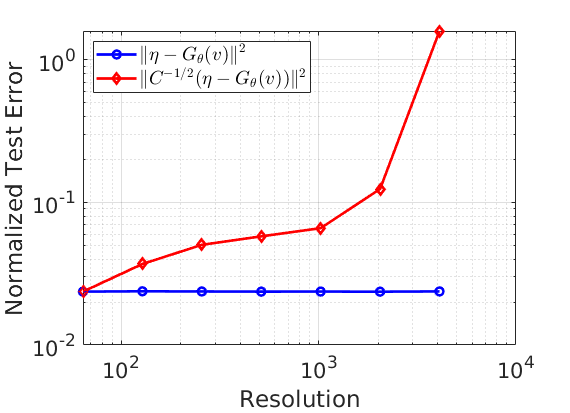
Figure 9: Noise Regularity  Test error when training with two different loss functions across different resolutions. Red curve is re-scaled so that it matches the error of the blue curve at the lowest resolution for the sake of visualization.

Appendix I Smoothing Operators

To illustrate the effect of the choice of the Camerion-Martin space (CM-space) of a (forward) noise process, we train an FNO architecture with varying training conditions. Specifically, we simulate that samples from data distribution, $u\sim\mu$, which may or may not be in the noise’s CM-space.

Similar to Section F.1, we consider a mixture of two Gaussians as data distribution $\mu$ where $d=1$, $D=(0,2\pi)$, $f_{1}=-10/6x+5$, $f_{2}=-f_{1}$, and $p=0.5$. For its covariance $C_{1}$, we choose $\alpha_{1}=1.5$, $\sigma_{1}=3$, and $\tau_{1}=3$.

We compare four training conditions by varying the noise covariance $C_{2}$; (a) noise process uses white noise, (b) all data samples lie on the CM-space of the noise covariance, (c) there exist samples $u\notin C_{2}^{1/2}(H)$, and (d) apply a smoothing operator $A$, while the same covariance as in (c). For (b), we choose $\alpha_{1}=1$, $\sigma_{1}=1.73$, and $\tau_{1}=3$, and for (c) and (d), we use $\alpha_{1}=2$, $\sigma_{1}=10$, and $\tau_{1}=3$. For smoothing operator $A$ in (d), we use a Gaussian blur such that $A(H)\subseteq C_{2}^{1/2}(H)$.

We train models at a resolution of $512$ for $5,000$ iterations. Unlike Section F.1, we only trained in the resolution $512$ and sample with varying resolutions (See Figure 10).

From (a), we can observe that the trained model successfully generates the samples in resolution 512, the same resolution during training. However, when the trained model tries to generate higher-resolution samples, its samples collapse into modes. While the parametric score operator is discretization-invariant, due to independent Gaussian noise, the induced distribution from the model is not in function-valued space.

On the contrary, when $C_{2}^{1/2}(H)$ is sufficiently large enough to include all samples from the data distribution, the proposed method learns the data distribution. Moreover, the model successfully generates samples in higher dimensions, as the model distribution is a measure in a function-valued space.

If samples are not in $C_{2}^{1/2}(H)$, the model fails to learn the data distribution as in Figure 10 (c). As we discussed in Section 4.3, however, one can apply a smoothing operator $A$ so that $A(H)\subseteq C_{2}^{1/2}(H)$. This results in losing some information about the data, depending on the choice of the smoothing operator. Here, high-frequency noises are cut out as we use a Gaussian blur.

The results demonstrate that the proposed method will learn the distributions in function space; thus, it is discretization invariant. Moreover, the result further implies that the choice of noise process and smoothing operator will determine which perspectives of data distributions the models will learn. Furthermore, the experiment led to several open questions for choosing noising processes most suitable for applications.

()

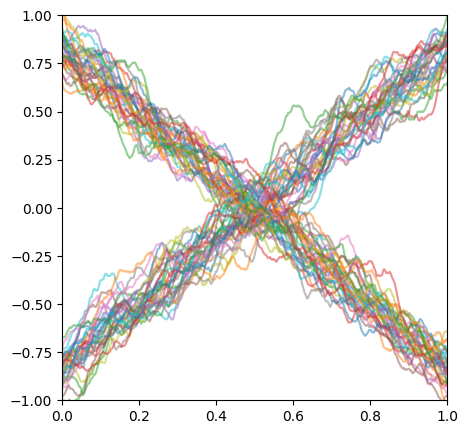
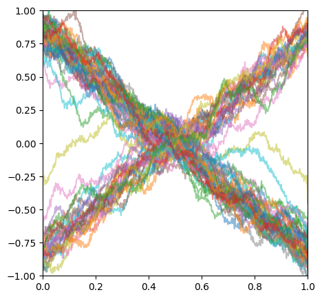
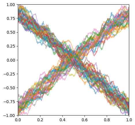
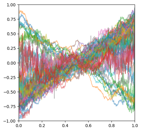
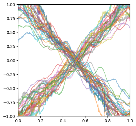
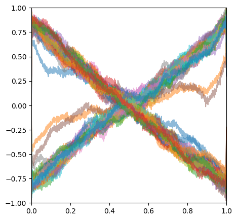
(a)

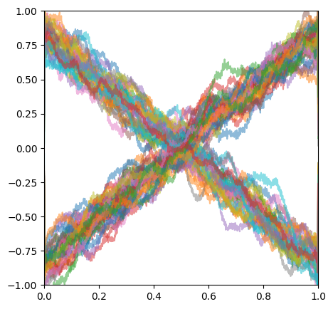
(b)

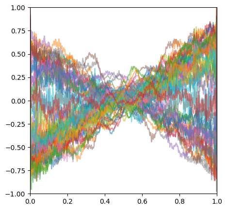
(c)

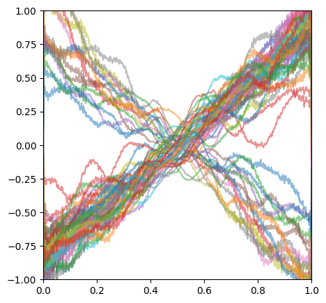
(d)

Figure 10: Smoothing Operators (Section 4.3) First row illustrates 128 sample paths from the data distribution $\mu$, a Mixture of two Gaussians. The second and third row illustrate generated samples from trained models. We train a FNO architecture with varying choice of the noise’ covariance $C_{2}$; (a) independent Gaussian noise process, (b) for all $u\in\mu$, $u\in C_{2}^{1/2}(H)$, (c) $\exists\,u\notin C_{2}^{1/2}(H)$, and (d) apply a smoothing operator while the same covariance as in (c). For smoothing operator $A$ in (d), we use a Gaussian blur such that $A(H)\subseteq C_{2}^{1/2}(H)$. The models are trained in a $512$ resolution, and generate with varying resolutions, such as $512$ (Second row) and $2048$ (Third row).

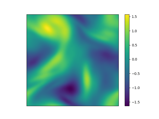
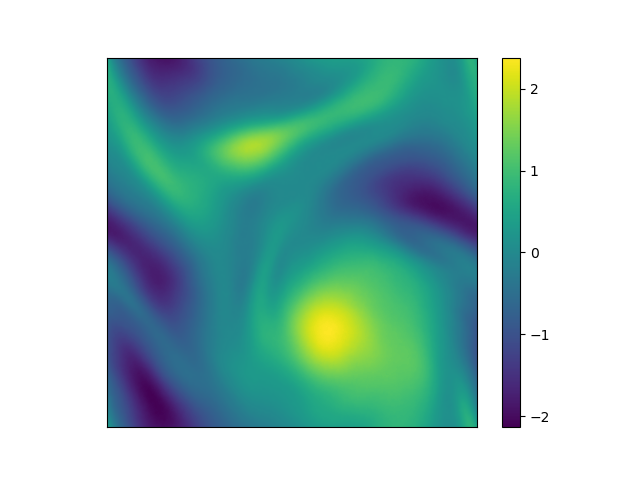
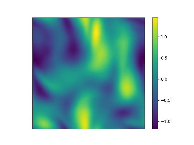
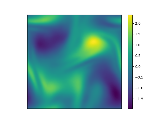
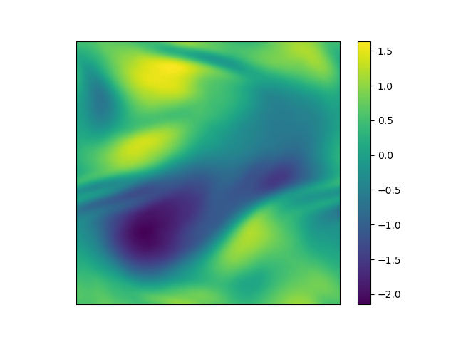
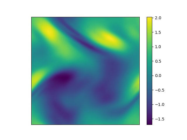
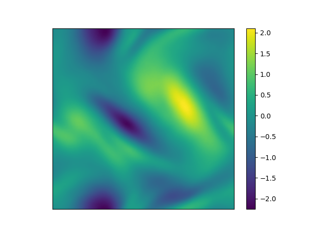
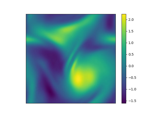
Figure 11: Navier-Stokes. Uncurated samples at the resolution $1024\times 1024$ from our diffusion model trained on a dataset at the resolution $128\times 128$.

Appendix J Experimental Details

In all examples we train by picking $\mathcal{{I}}=[10]$ and sample with Algorithm 1 by fixing $M=200$ and $\epsilon=2\times 10^{-5}$. We choose $\sigma_{1}=1.0$ and $\sigma_{10}=0.01$ with all other $\sigma$ parameters defined by a geometric sequence. We train with a combined loss defined by (16) where we re-scale the the noise by $\sigma_{t}^{-1}$ and the score by $\sigma_{t}$, following Song and Ermon (2019). In particular, our model learns to approximate $v\mapsto\sigma_{t}^{-2}\big{(}RD_{H_{\mu_{t}}}\Phi(u,t)-v\big{)}$. Note that the $\sigma_{t}^{-2}$ term is canceled by the adaptive time-step in Algorithm 1, however, as in Song and Ermon (2019), we find that this re-scaling significantly improves performance for all models. We leave a theoretical analysis of this for future work. To be explicit, our loss function is

$$\min_{\theta}\frac{1}{|\mathcal{{I}}|}\sum_{t\in\mathcal{{I}}}\mathbb{E}_{u\sim\mu}\mathbb{E}_{\eta_{t}\sim\mu_{t}}\left\|\frac{\eta_{t}}{\sigma_{t}}+\sigma_{t}F_{\theta}(u+\eta_{t},t)\right\|^{2}$$

where $\|\cdot\|$ is the $L^{2}(D;\mathbb{{R}})$ norm and $D$ is problem-dependent. We train with the Adam optimizer for a total of $300$ epochs and an initial learning rate $10^{-3}$, which is decayed by half every $50$ epochs.

J.1 Gaussian Mixture

We consider the problem setting of Section F.1 with $d=1$ and $D=(0,2\pi)$. We pick $f_{1}=\sin(x/2)$ and $f_{2}=-f_{1}$ as well as $p=0.5$. We generate $N=10,000$ samples for training at a resolution of $2048$ and subsample these to obtain all other datasets. For the data covariance $C_{1}$, we choose $\alpha_{1}=3$, $\sigma_{1}=3$, and $\tau_{1}=3$, and, for the noise covariance $C_{2}$, we choose $\alpha_{1}=0.6$, $\sigma_{1}=0.5$, and $\tau_{1}=0.1$. We train with a FNO architecture wich retains 48 modes and has a width of 128. We re-train the model at each separate resolution. In Figure 12 we visualize samples from each of the models trained with white noise as well as the trace-class noise with covariance $C_{2}$ at the resolutions $64,512$, and $2048$. We point out that the models trained at high resolutions with white noise completely fail to capture the right distribution.

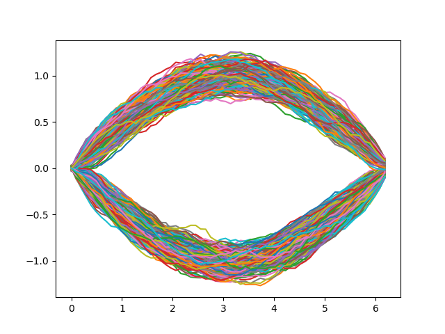
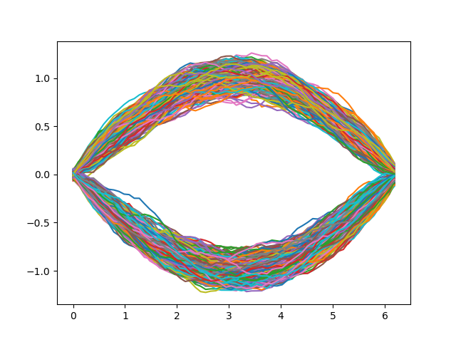
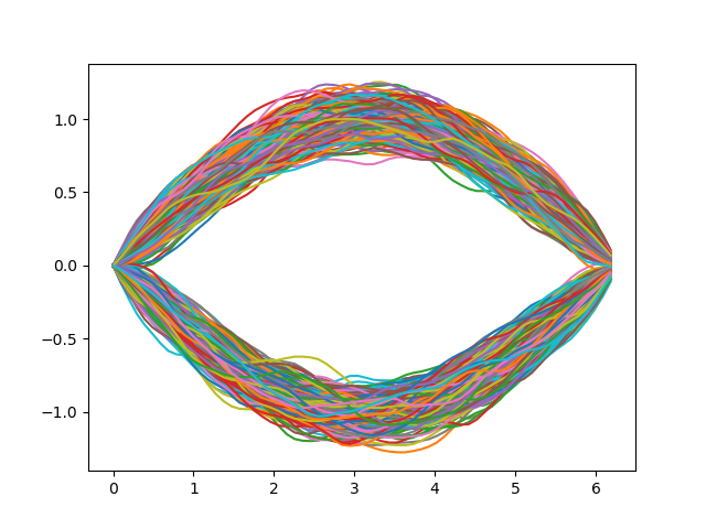
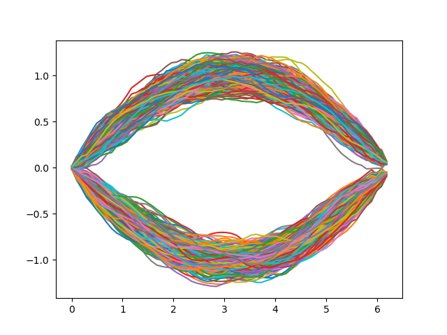
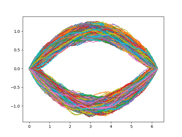
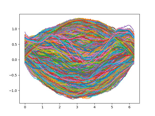
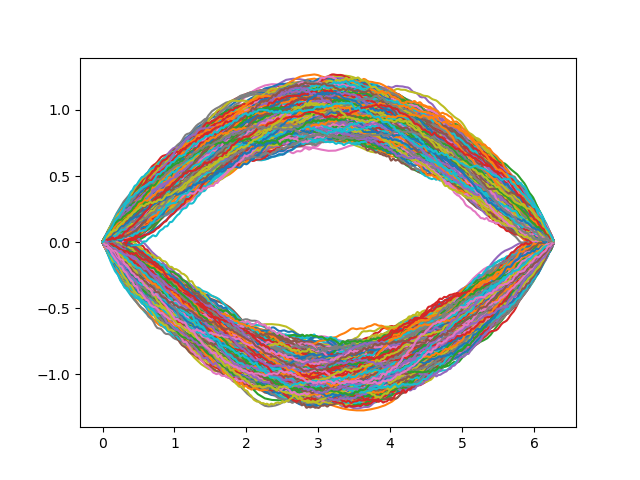
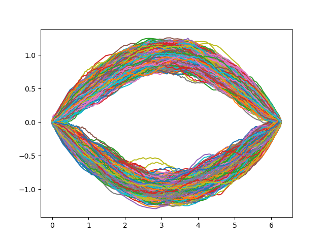
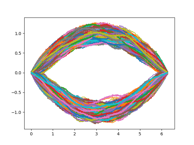
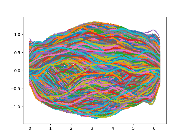
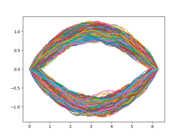
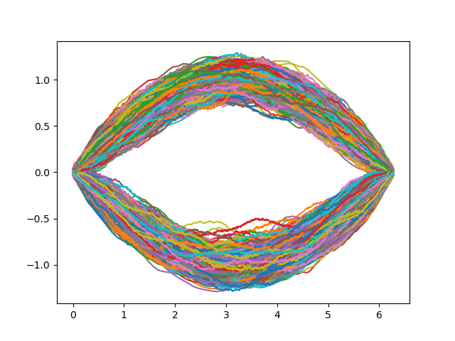
Figure 12: Guassian mixture. Each row represents the resolutions $64,512,2048$ respectively. The first and third columns show samples from $\nu_{T}$ (the perturbed data measure with the smallest amount of noise added) for the white noise and trace-class noise respectively. The second and fourth columns show samples generated from the trained model using white noise and trace-class noise respectively.

J.2 Navier-Stokes

We consider a problem setting similar to Section F.2.1. We fix the initial condition $u(\cdot,0)=0$ and instead generate random forcings $f$ from the Gaussian $\rho$. The same theory as in Section F.2.1 still applies and the pushforward is non-Gaussian due to the non-linearity of the PDE. We solve it up to the final time $T=5$ with the pseudo-spectral scheme of Chandler and Kerswell (2013) with $\epsilon=1/500$ and $N=10,000$ samples for training. We pick $\alpha_{1}=4$, $\sigma_{1}=3\sqrt{3}$ and $\tau_{1}=3$ for the reference Gaussian $\rho$, following (De Hoop et al., 2022). All data is generated with a $1024\times 1024$ resolution and the $128\times 128$ is created from it by sub-sampling. With train our mode with a FNO architecture retaining $80\times 80$ modes with a width of $64$. We pick the parameters $\alpha_{2}=1.5$, $\sigma_{2}=4$, and $\tau_{2}=5$ for our noise covariance. In Figure 11, we show more samples generated by the model, performing zero-shot super-resolution.

J.3 Volcano Dataset

For the volcano experiments, we use the loss formulation from Equation (16) but employ a noise schedule $\{\sigma_{1},\dots,\sigma_{L}\}$ (as is standard with SBGMs). Inspired by Song and Ermon (2020) we optimize a weighted variant of it where $F_{\theta}$ is preconditioned with $\sigma_{i}$:

$$\min_{\theta\in\mathbb{R}^{p}}\mathbb{E}_{u\sim\mu}\mathbb{E}_{\eta_{i}}\|\eta_{i}+\sigma_{i}F_{\theta}(u+\eta_{i},\sigma_{i})\|^{2}$$ (38a)

$$= \min_{\theta\in\mathbb{R}^{p}}\mathbb{E}_{u\sim\mu}\mathbb{E}_{\epsilon\sim\mathcal{N}(0,\mathbf{I})}\mathbb{E}_{i\sim U(1,L)}\|\mathbf{L}_{i}\epsilon+\sigma_{i}F_{\theta}(u+\mathbf{L}_{i}\epsilon,\sigma_{i})\|^{2}$$ (38b)

$$= \min_{\theta\in\mathbb{R}^{p}}\mathbb{E}_{u\sim\mu}\mathbb{E}_{\epsilon\sim\mathcal{N}(0,\mathbf{I})}\mathbb{E}_{i\sim U(1,L)}\|\sigma_{i}\mathbf{L}\epsilon+\sigma_{i}F_{\theta}(u+\sigma_{i}\mathbf{L}\epsilon,\sigma_{i})\|^{2},$$ (38c)

$$= \min_{\theta\in\mathbb{R}^{p}}\mathbb{E}_{u\sim\mu}\mathbb{E}_{\epsilon\sim\mathcal{N}(0,\mathbf{I})}\mathbb{E}_{i\sim U(1,L)}\|\sigma_{i}\big{(}\mathbf{L}\epsilon+F_{\theta}(u+\sigma_{i}\mathbf{L}\epsilon,\sigma_{i})\big{)}\|^{2}$$ (38d)

where $\eta_{i}\sim\mathcal{N}(0,\mathbf{C}_{i}^{2})=\mathcal{N}(0,\sigma_{i}^{2}\mathbf{C}^{2})$, and via the reparameterisation trick this can be re-written as $\eta_{i}=\sigma_{i}\mathbf{L}\epsilon$, where $\mathbf{L}=\text{chol}(\mathbf{C})$ and $\epsilon\sim\mathcal{N}(0,\mathbf{I})$. Here, we use a covariance computed using the RBF kernel over a 2D meshgrid representing the coordinates of the image (function):

$$\mathbf{C}(x)_{ij}=\exp\Big{(}-\frac{\|x_{i}-x_{j}\|^{2}}{2\gamma^{2}}\Big{)},\ \,i,j\in\{1,\dots,s^{2}\}$$ (39)

where $x\in[0,1]^{s^{2}\times 2}$ for a spatial resolution of $s$, and $\mathbf{C}\in\mathbb{R}^{s^{2}\times s^{2}}$. The hyperparameter $\gamma$ controls the smoothness of the noise, with larger values indicating higher levels of smoothness. Example sample noises are illustrated in Figure 13.

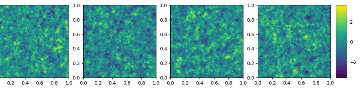
(a) $\gamma=0.1$.

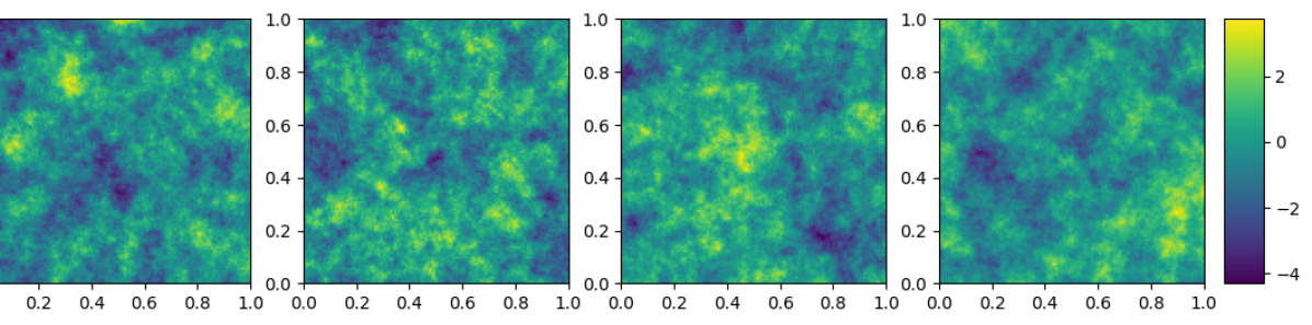
(b) $\gamma=0.2$.

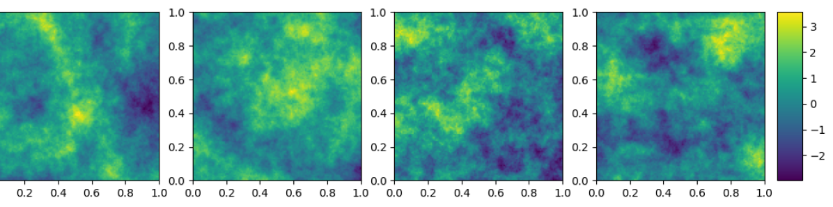
(c) $\gamma=0.3$.

Figure 13: Samples with RBF kernels: Sample noises for varying smoothness parameters $\gamma$ of RBF kernels.

As suggested in Song and Ermon (2020), we redefine $F_{\theta}(\cdot,\sigma)=F_{\theta}(\cdot)/\sigma$ since the authors noted that this makes the noise prediction task more robust to a wide range of noise scales.

Architecture

The architecture we use is a U-shaped neural operator (UNO). This architecture consists of a series of Fourier neural operator blocks (FNOBlocks) which progressively downsample or upsample the input. We use the implementation of FNOBlocks from the Neural Operators library Li et al. (2020a); Kovachki et al. (2021b). Concretely, for the Volcano dataset the example $u$ has a spatial dimension of $120\times 120$ with two channels, and is lifted from $2\rightarrow 128$ channels with a preprocessing convolutional layer, which also pads the 120 pixel image (function) to 128 pixels. Afterwards, the lifted input is run through four FNOBlocks which progressively lift the channel dimension and spatial dimensions to $(128\rightarrow 256\rightarrow 512\rightarrow 512)$ and $(128\rightarrow 96\rightarrow 64\rightarrow 32)$, respectively. A similar set of blocks is used in the decoder block along with skip connections.

For FNOBlock, we use Tucker factorisation with a rank of 0.1. In order to ensure the number of learnable parameters does not explode, we also constrain the number of Fourier modes in each FNOBlock to be 50% of the number of input channel dimensions for each block. The resulting U-shaped neural operator contains a total of  142M learnable parameters.

Training Details

We train the models using ADAM Kingma and Ba (2014) with default moving average hyperparameters $\beta=(0.9,0.999)$, with a learning rate of $2e^{-4}$. For the noise schedule, we employ a geometric schedule using $(\sigma_{1},\sigma_{L})=(30,0.01)$, for $L=500$ time steps. The number of SGLD iterations per timestep is $T=3$ and we use a step size of $6e^{-6}$. At generation time, we use annealed SGLD and run the Markov chain on $u_{0}\sim\mathcal{N}(0,\mathbf{C})$.

Hyperparameters

We use circular skewness and circular variance, moments of circular variables which were originally proposed in GANO (Rahman et al., 2022) Given an image (function) $u\in\mathbb{R}^{s^{2}\times 2}$ we can define its angle as $\theta=\text{atan2}(u_{:,1},u_{:,2})$. If we define $R_{p}(\theta)=\frac{1}{s^{2}}\sqrt{z_{p}(\theta)}$ for $z_{p}(\theta)=(\sum_{k}^{s^{2}}(\cos(p\theta_{k})+i\sin(p\theta_{k}))^{2}$ and $\varphi_{p}(\theta)=\text{arg}(z_{p}(\theta))$ (for $s^{2}$ spatial dimensions) then:

$$w_{\text{var}}(\theta)=1-R_{1}(\theta),\ \ \ w_{\text{skew}}(\theta)=\frac{R_{2}(\theta)\sin(\varphi_{2}(\theta)-2\varphi_{1}(\theta))}{(1-R_{1}(\theta))^{3/2}}$$ (40)

where $i=\sqrt{-1}$ and $k$ is a summation over the spatial dimensions $s^{2}$.

J.4 MNIST-SDF Dataset

For the noising processes in the MNIST-SDF experiments, we adopt Equation 32 in Appendix E. More specifically, we follow a more generalized formulation described in Kingma et al. (2021). For $t\in(0,1]$, we first define $u_{t}$s as in,

$$u_{t}=\alpha_{t}u+\sigma_{t}\eta,$$ (41)

where $\eta\sim\mu_{0}=N(0,C)$ and $u\sim\mu$. In this experiment, we use variance-preserving setting for the forward process; thus, $\alpha_{t}$ and $\sigma_{t}$ will satisfy $\alpha_{t}^{2}+\sigma_{t}^{2}=1$ for $t\in[0,1]$. The approximate backwards conditional in Equation 34 will be re-written as $u_{s}|u_{t}$ for $\forall\,s,t\,$ s.t. $0<s<t\leq 1$;

$$u_{s}=M_{\theta}(u_{t},t)+\sigma_{\textup{back},s,t}\eta,$$ (42)

where $\eta\sim\mu_{0}$. $M_{\theta}$ and $\sigma_{\textup{back},s,t}$ are written as

$$M_{\theta}(u_{t},t) =\frac{\alpha_{t\,\rule{0.6pt}{3.01389pt}\,s}\sigma_{s}^{2}}{\sigma_{t}^{2}}u_{t}-\frac{\alpha_{s\,\rule{0.6pt}{3.01389pt}\,t}\sigma_{t\,\rule{0.6pt}{3.01389pt}\,s}^{2}}{\sigma_{t}^{2}}\left(u_{t}-\sigma_{t}F_{\theta}(u_{t},t)\right)$$ (43)

$$\sigma_{\textup{back},s,t} =\frac{\sigma_{t\,\rule{0.6pt}{3.01389pt}\,s}^{2}\sigma_{s}^{2}}{\sigma_{t}^{2}},$$ (44)

where $\alpha_{t\,\rule{0.6pt}{3.01389pt}\,s}=\alpha_{t}/\alpha_{s}$ and $\sigma_{t\,\rule{0.6pt}{3.01389pt}\,s}=\sigma_{t}^{2}-\alpha_{t\,\rule{0.6pt}{3.01389pt}\,s}^{2}\sigma_{s}^{2}$.

The aforementioned formulations provide us several benefits. Most importantly, we can choose arbitrary sequence of discrete time steps in order to generate the learned distribution. This implies that we can train $F_{\theta}$ at all $t\in(0,1]$ and choose the sampling sequence later after training. As a result, instead of the training loss Equation 33, we obtimize the following objective,

$$\mathbb{{E}}_{u\sim\mu,\eta\sim\mu_{0},t\sim U(0,1)}\|F_{\theta}\big{(}\alpha_{t}u+\sigma_{t}\eta,t\big{)}-\eta\|^{2}.$$ (45)

In the following sections, we will continue on the trace-class noises used in the experiments and other details.

GRFs with $p$-th Order Exponential Covariance Functions

We observe that the models often generate artifacts with the blurring diffusions when the noise process is non-periodic Gaussian measures (Section 4.2), as the Gaussian smoothing operator is periodic. Thus, we use periodic Gaussian measures with $p$-th order exponential covariance function, whose kernel function is written as,

$$k(x,x^{\prime})=\sigma\exp\left(-\left|\frac{x-x^{\prime}}{l}\right|^{p}\right),$$ (46)

where $l$ is a length scale, $p$ is order, and $\sigma$ is a magnitude. Note that the RBF kernel used in the volcano experiments is a special case of Equation 46

As the data is assumed to be sampled on a lattice in $\mathbb{R}^{d}$, we employ the convolution construction of the Gaussian measures for efficient sampling (Higdon, 2002). For a given exponential kernel $k$, the corresponding convolution kernel $c$ is a function of the absolute difference $x$ and is written as

$$c(x)=\mathcal{F}^{-1}\left[\sqrt{\mathcal{F}[k]}\right](x)$$

where $\mathcal{F}$ and $\mathcal{F}^{-1}$ are Fourier and inverse Fourier transform, respectively. We denote the closed form $\mathcal{F}(k)(\omega)$ for $p$-th order exponential kernel as $\phi_{p}(\omega)$, and $\phi_{p}$ is written as

$$\phi_{p}(\omega)=\begin{cases}\frac{2}{1+\omega^{2}},&p=1,\\ 2\pi c_{p}\frac{p|\omega|^{\frac{1}{1-p}}}{2|p-1|}\int_{0}^{1}U_{p}(x)\exp\left(-|\omega|^{\frac{p}{p-1}}U_{p}(x)\right)dx,&p\in(0,2]\setminus\{1\},\\ \end{cases}$$

where $c_{p}$ and $U_{p}$ are defined as

$$c_{p}=\frac{p}{2^{\frac{p+1}{p}}\Gamma\left(\frac{1}{p}\right)}\quad\,\,\textrm{and}\quad\,\,U_{p}(x)=\left(\frac{\sin\left(\frac{\pi xp}{2}\right)}{\cos\left(\frac{\pi x}{2}\right)}\right)^{\frac{p}{1-p}}\frac{\cos\left(\frac{\pi x(p-1)}{2}\right)}{\cos\left(\frac{\pi x}{2}\right)},$$

and $\Gamma$ is the Gamma function. The detailed information about $\phi_{p}$, including its derivation, is described in Dytso et al. (2018).

Architecture and Training Details

This section provides a detailed description of the experimental configuration used in our study. Before elaborating on the hyperparameters, we introduce a neural operator in the image experiments. We modify the UNet network architectures (Ronneberger et al., 2015), which has been widely adopted in the context of diffusion-based generative models (Ho et al., 2020; Song et al., 2020b; Nichol and Dhariwal, 2021) and elaborated with regards to neural operators (Rahman et al., 2022, 2023). We adopt the Improved Denoising Diffusion Probabilistic Models (IDDPM, Nichol and Dhariwal 2021), whose time-conditional modulation uses elementwise affine transformations (shift and scale) instead of shifting-only modulation introduced in Ho et al. (2020). To do that, we introduce four major modifications. First, we replace all regular convolutional layers with spectral convolutions. Second, we apply group normalizations on Fourier spaces instead of Euclidean spaces. Here, the normalization coefficients will be computed using the first $k$ modes in Fourier spaces, but the coefficient will be applied to all modes; thus, the normalization works in a resolution-invariant manner. Third, we deprecate the self-attention layers and dropouts. Moreover, for the downsample and upsample operations, which are one of the key components of the UNet-like hierarchical network architectures, we adopt filtered downsample and upsample algorithms discussed in Karras et al. (2021). Therefore, we conclude that the resulting deep learning architecture is a valid neural operator as it is a combination of convolutional operators, normalizations defined in Fourier spaces, and point-wise transformations.

Specifically for the MNIST-SDF experiment, we set the number of base channels to 64 and use the three-stage model. The channel multipliers for each stage are set to 1, 2, and 2, respectively. For each stage, four residual blocks are used. At the first stage, all spectral convolution layers comprise 32 modes, and we halve the modes as the stage increases.

We chose the cosine noise scheduling following IDDPM with a variance-preserving form for the noise schedule. We follow the sine schedule introduced in Hoogeboom and Salimans (2022) for the blurring schedule. We describe the hyperparameter details in the Table 3

Table 3: Training details of DDO for MNIST-SDF experiments

Architecture	Base channels	64
	# of ResBlocks per stage	4
	Channel multiplier	1,2,2
	# of modes per stage	32, 16, 8
	Activation function	GeLU‡
Diffusion	Noise schedule	Cosine
	$\log(\alpha_{0}^{2}/\sigma_{0}^{2})$	10
	$\log(\alpha_{1}^{2}/\sigma_{1}^{2})$	-10
Blurring	Blurring schedule	Sine
	$d_{0}$§	0.05
	$d_{1}$	0.25
Learning	Optimizer	Adam, $\beta_{1}$=0.9, $\beta_{2}$=0.999
	Learning rate	0.00001
	Batch size	32
	# of iterations	2M
Sampling	# of steps	250
§$d_{0}$ and $d_{1}$ are frequency scalings at $t=0$ and $d_{1}$, respectively.
‡Gaussian Error Linear Units function(Hendrycks and Gimpel, 2016).

References

- Adams and Fournier (2003) R.A. Adams and J.J.F. Fournier. Sobolev Spaces. ISSN. Elsevier Science, 2003. ISBN 9780080541297.
- Adler (2010) Robert J Adler. The geometry of random fields. SIAM, 2010.
- Anokhin et al. (2021) Ivan Anokhin, Kirill Demochkin, Taras Khakhulin, Gleb Sterkin, Victor Lempitsky, and Denis Korzhenkov. Image generators with conditionally-independent pixel synthesis. In Proceedings of the IEEE/CVF Conference on Computer Vision and Pattern Recognition, pages 14278–14287, 2021.
- Arjovsky and Bottou (2017) Martin Arjovsky and Léon Bottou. Towards principled methods for training generative adversarial networks. arXiv preprint arXiv:1701.04862, 2017.
- Baldassari et al. (2023) Lorenzo Baldassari, Ali Siahkoohi, Josselin Garnier, Knut Solna, and Maarten V de Hoop. Conditional score-based diffusion models for bayesian inference in infinite dimensions. arXiv preprint arXiv:2305.19147, 2023.
- Bautista et al. (2022) Miguel Angel Bautista, Pengsheng Guo, Samira Abnar, Walter Talbott, Alexander Toshev, Zhuoyuan Chen, Laurent Dinh, Shuangfei Zhai, Hanlin Goh, Daniel Ulbricht, et al. Gaudi: A neural architect for immersive 3d scene generation. arXiv preprint arXiv:2207.13751, 2022.
- Berard et al. (2020) Hugo Berard, Gauthier Gidel, Amjad Almahairi, Pascal Vincent, and Simon Lacoste-Julien. A closer look at the optimization landscapes of generative adversarial networks. In International Conference on Machine Learning (ICML), 2020.
- Bogachev (2015) V.I. Bogachev. Gaussian Measures. Mathematical Surveys and Monographs. American Mathematical Society, 2015. ISBN 9781470418694.
- Bruinsma et al. (2021) Wessel P Bruinsma, James Requeima, Andrew YK Foong, Jonathan Gordon, and Richard E Turner. The gaussian neural process. arXiv preprint arXiv:2101.03606, 2021.
- Chandler and Kerswell (2013) Gary J. Chandler and Rich R. Kerswell. Invariant recurrent solutions embedded in a turbulent two-dimensional kolmogorov flow. Journal of Fluid Mechanics, 722:554–595, 2013.
- Chen et al. (2021) Yinbo Chen, Sifei Liu, and Xiaolong Wang. Learning continuous image representation with local implicit image function. In Proceedings of the IEEE/CVF conference on computer vision and pattern recognition, pages 8628–8638, 2021.
- Chou et al. (2022) Gene Chou, Yuval Bahat, and Felix Heide. Diffusionsdf: Conditional generative modeling of signed distance functions. arXiv preprint arXiv:2211.13757, 2022.
- Cotter et al. (2013) Simon L Cotter, Gareth O Roberts, Andrew M Stuart, and David White. Mcmc methods for functions: modifying old algorithms to make them faster. Statistical Science, 28(3):424–446, 2013.
- Craswell (1965) KJ Craswell. Density estimation in a topological group. The Annals of Mathematical Statistics, 36(3):1047–1048, 1965.
- Da Prato et al. (1992) G. Da Prato, G. De Prato, and J. Zabczyk. Stochastic Equations in Infinite Dimensions. Encyclopedia of Mathematics and its Applications. Cambridge University Press, 1992. ISBN 9780521385299.
- Da Prato (2006) Giuseppe Da Prato. An introduction to infinite-dimensional analysis. Springer Science & Business Media, 2006.
- Dabo-Niang (2004) Sophie Dabo-Niang. Kernel density estimator in an infinite-dimensional space with a rate of convergence in the case of diffusion process. Applied mathematics letters, 17(4):381–386, 2004.
- Dashti and Stuart (2017) Masoumeh Dashti and Andrew M Stuart. The bayesian approach to inverse problems. In Handbook of uncertainty quantification, pages 311–428. Springer, 2017.
- De Hoop et al. (2022) Maarten De Hoop, Daniel Zhengyu Huang, Elizabeth Qian, and Andrew M Stuart. The cost-accuracy trade-off in operator learning with neural networks. arXiv preprint arXiv:2203.13181, 2022.
- Dupont et al. (2021) Emilien Dupont, Yee Whye Teh, and Arnaud Doucet. Generative models as distributions of functions. arXiv preprint arXiv:2102.04776, 2021.
- Dupont et al. (2022) Emilien Dupont, Hyunjik Kim, S. M. Ali Eslami, Danilo Jimenez Rezende, and Dan Rosenbaum. From data to functa: Your data point is a function and you can treat it like one. In Kamalika Chaudhuri, Stefanie Jegelka, Le Song, Csaba Szepesvari, Gang Niu, and Sivan Sabato, editors, Proceedings of the 39th International Conference on Machine Learning, volume 162 of Proceedings of Machine Learning Research, pages 5694–5725. PMLR, 17–23 Jul 2022.
- Dutordoir et al. (2022) Vincent Dutordoir, Alan Saul, Zoubin Ghahramani, and Fergus Simpson. Neural diffusion processes. arXiv preprint arXiv:2206.03992, 2022.
- Dytso et al. (2018) Alex Dytso, Ronit Bustin, H Vincent Poor, and Shlomo Shamai. Analytical properties of generalized gaussian distributions. Journal of Statistical Distributions and Applications, 5(1):1–40, 2018.
- Evans (2010) Lawrence C. Evans. Partial differential equations. American Mathematical Society, 2010.
- Föllmer and Wakolbinger (1986) H Föllmer and A Wakolbinger. Time reversal of infinite-dimensional diffusions. Stochastic processes and their applications, 22(1):59–77, 1986.
- Garnelo et al. (2018) Marta Garnelo, Jonathan Schwarz, Dan Rosenbaum, Fabio Viola, Danilo J Rezende, SM Eslami, and Yee Whye Teh. Neural processes. arXiv preprint arXiv:1807.01622, 2018.
- Gelbrich (1990) Matthias Gelbrich. On a formula for the l2 wasserstein metric between measures on euclidean and hilbert spaces. Mathematische Nachrichten, 147(1):185–203, 1990.
- Ghosal and van der Vaart (2017) S. Ghosal and A. van der Vaart. Fundamentals of Nonparametric Bayesian Inference. Cambridge Series in Statistical and Probabilistic Mathematics. Cambridge University Press, 2017. ISBN 9780521878265.
- Goodfellow et al. (2020) Ian Goodfellow, Jean Pouget-Abadie, Mehdi Mirza, Bing Xu, David Warde-Farley, Sherjil Ozair, Aaron Courville, and Yoshua Bengio. Generative adversarial networks. Communications of the ACM, 63(11):139–144, 2020.
- Guth et al. (2022) Florentin Guth, Simon Coste, Valentin De Bortoli, and Stephane Mallat. Wavelet score-based generative modeling. arXiv preprint arXiv:2208.05003, 2022.
- Hagemann et al. (2023) Paul Hagemann, Lars Ruthotto, Gabriele Steidl, and Nicole Tianjiao Yang. Multilevel diffusion: Infinite dimensional score-based diffusion models for image generation. arXiv preprint arXiv:2303.04772, 2023.
- Halmos (1976) P.R. Halmos. Measure Theory. Graduate Texts in Mathematics. Springer New York, 1976. ISBN 9780387900889.
- Hendrycks and Gimpel (2016) Dan Hendrycks and Kevin Gimpel. Gaussian error linear units (gelus). arXiv preprint arXiv:1606.08415, 2016.
- Heusel et al. (2017) Martin Heusel, Hubert Ramsauer, Thomas Unterthiner, Bernhard Nessler, and Sepp Hochreiter. Gans trained by a two time-scale update rule converge to a local nash equilibrium. Neural Information Processing Systems (NeurIPS), 2017.
- Higdon (2002) Dave Higdon. Space and space-time modeling using process convolutions. In Quantitative methods for current environmental issues, pages 37–56. Springer, 2002.
- Ho et al. (2020) Jonathan Ho, Ajay Jain, and Pieter Abbeel. Denoising diffusion probabilistic models. Neural Information Processing Systems (NeurIPS), 2020.
- Hoogeboom and Salimans (2022) Emiel Hoogeboom and Tim Salimans. Blurring diffusion models. In International Conference on Learning Representations (ICLR), 2022.
- Hui et al. (2022) Ka-Hei Hui, Ruihui Li, Jingyu Hu, and Chi-Wing Fu. Neural wavelet-domain diffusion for 3d shape generation. In SIGGRAPH Asia 2022 Conference Papers, pages 1–9, 2022.
- Hyvärinen (2005) Aapo Hyvärinen. Estimation of non-normalized statistical models by score matching. Journal of Machine Learning Research, 6(24):695–709, 2005. URL http://jmlr.org/papers/v6/hyvarinen05a.html.
- Jing et al. (2022) Bowen Jing, Gabriele Corso, Renato Berlinghieri, and Tommi Jaakkola. Subspace diffusion generative models. arXiv preprint arXiv:2205.01490, 2022.
- Karras et al. (2021) Tero Karras, Miika Aittala, Samuli Laine, Erik Härkönen, Janne Hellsten, Jaakko Lehtinen, and Timo Aila. Alias-free generative adversarial networks. Neural Information Processing Systems (NeurIPS), 2021.
- Kerrigan et al. (2022) Gavin Kerrigan, Justin Ley, and Padhraic Smyth. Diffusion generative models in infinite dimensions. arXiv preprint arXiv:2212.00886, 2022.
- Kim et al. (2021) Dongjun Kim, Seungjae Shin, Kyungwoo Song, Wanmo Kang, and Il-Chul Moon. Soft truncation: A universal training technique of score-based diffusion model for high precision score estimation. arXiv e-prints, pages arXiv–2106, 2021.
- Kim et al. (2019) Hyunjik Kim, Andriy Mnih, Jonathan Schwarz, Marta Garnelo, Ali Eslami, Dan Rosenbaum, Oriol Vinyals, and Yee Whye Teh. Attentive neural processes. arXiv preprint arXiv:1901.05761, 2019.
- Kingma et al. (2021) Diederik Kingma, Tim Salimans, Ben Poole, and Jonathan Ho. Variational diffusion models. Neural Information Processing Systems (NeurIPS), 2021.
- Kingma and Ba (2014) Diederik P Kingma and Jimmy Ba. Adam: A method for stochastic optimization. arXiv preprint arXiv:1412.6980, 2014.
- Kiselev et al. (2008) Alexander Kiselev, Fedor Nazarov, and Roman Shterenberg. Blow up and regularity for fractal burgers equation. arXiv preprint arXiv:0804.3549, 2008.
- Kong et al. (2020) Zhifeng Kong, Wei Ping, Jiaji Huang, Kexin Zhao, and Bryan Catanzaro. Diffwave: A versatile diffusion model for audio synthesis. arXiv preprint arXiv:2009.09761, 2020.
- Kovachki et al. (2021a) Nikola Kovachki, Samuel Lanthaler, and Siddhartha Mishra. On universal approximation and error bounds for fourier neural operators. Journal of Machine Learning Research, 22(290):1–76, 2021a.
- Kovachki et al. (2021b) Nikola Kovachki, Zongyi Li, Burigede Liu, Kamyar Azizzadenesheli, Kaushik Bhattacharya, Andrew Stuart, and Anima Anandkumar. Neural operator: Learning maps between function spaces. arXiv preprint arXiv:2108.08481, 2021b.
- Kupiainen (2016) Antti Kupiainen. Quantum fields and probability. arXiv preprint arXiv:1611.05240, 2016.
- Kynkäänniemi et al. (2019) Tuomas Kynkäänniemi, Tero Karras, Samuli Laine, Jaakko Lehtinen, and Timo Aila. Improved precision and recall metric for assessing generative models. Neural Information Processing Systems (NeurIPS), 2019.
- Li et al. (2022) Xiang Lisa Li, John Thickstun, Ishaan Gulrajani, Percy Liang, and Tatsunori B Hashimoto. Diffusion-lm improves controllable text generation. arXiv preprint arXiv:2205.14217, 2022.
- Li et al. (2020a) Zongyi Li, Nikola Kovachki, Kamyar Azizzadenesheli, Burigede Liu, Kaushik Bhattacharya, Andrew Stuart, and Anima Anandkumar. Fourier neural operator for parametric partial differential equations. arXiv preprint arXiv:2010.08895, 2020a.
- Li et al. (2020b) Zongyi Li, Nikola Kovachki, Kamyar Azizzadenesheli, Burigede Liu, Kaushik Bhattacharya, Andrew Stuart, and Anima Anandkumar. Neural operator: Graph kernel network for partial differential equations. arXiv preprint arXiv:2003.03485, 2020b.
- Li et al. (2021) Zongyi Li, Nikola Kovachki, Kamyar Azizzadenesheli, Burigede Liu, Kaushik Bhattacharya, Andrew Stuart, and Anima Anandkumar. Learning dissipative dynamics in chaotic systems. arXiv preprint arXiv:2106.06898, 2021.
- Lin et al. (2018) Zinan Lin, Ashish Khetan, Giulia Fanti, and Sewoong Oh. Pacgan: The power of two samples in generative adversarial networks. In Neural Information Processing Systems (NeurIPS), 2018.
- Lindgren et al. (2011) Finn Lindgren, Håvard Rue, and Johan Lindström. An explicit link between gaussian fields and gaussian markov random fields: the stochastic partial differential equation approach. Journal of the Royal Statistical Society: Series B (Statistical Methodology), 73(4):423–498, 2011.
- Lord et al. (2014) Gabriel Lord, Catherine Powell, and Tony Shardlow. An Introduction to Computational Stochastic PDEs. 08 2014. ISBN 978-0521728522. doi:10.1017/CBO9781139017329.
- Mildenhall et al. (2021) Ben Mildenhall, Pratul P Srinivasan, Matthew Tancik, Jonathan T Barron, Ravi Ramamoorthi, and Ren Ng. Nerf: Representing scenes as neural radiance fields for view synthesis. Communications of the ACM, 65(1):99–106, 2021.
- Nelsen and Stuart (2021) Nicholas H Nelsen and Andrew M Stuart. The random feature model for input-output maps between banach spaces. SIAM Journal on Scientific Computing, 43(5):A3212–A3243, 2021.
- Nichol and Dhariwal (2021) Alexander Quinn Nichol and Prafulla Dhariwal. Improved denoising diffusion probabilistic models. In International Conference on Machine Learning (ICML), 2021.
- Nie et al. (2022) Weili Nie, Brandon Guo, Yujia Huang, Chaowei Xiao, Arash Vahdat, and Anima Anandkumar. Diffusion models for adversarial purification. In International Conference on Machine Learning (ICML), 2022.
- Park et al. (2019) Jeong Joon Park, Peter Florence, Julian Straub, Richard Newcombe, and Steven Lovegrove. Deepsdf: Learning continuous signed distance functions for shape representation. In Proceedings of the IEEE/CVF conference on computer vision and pattern recognition, pages 165–174, 2019.
- Pathak et al. (2022) Jaideep Pathak, Shashank Subramanian, Peter Harrington, Sanjeev Raja, Ashesh Chattopadhyay, Morteza Mardani, Thorsten Kurth, David Hall, Zongyi Li, Kamyar Azizzadenesheli, et al. Fourcastnet: A global data-driven high-resolution weather model using adaptive fourier neural operators. arXiv preprint arXiv:2202.11214, 2022.
- Phillips et al. (2022) Angus Phillips, Thomas Seror, Michael Hutchinson, Valentin De Bortoli, Arnaud Doucet, and Emile Mathieu. Spectral diffusion processes. arXiv preprint arXiv:2209.14125, 2022.
- Pidstrigach et al. (2023) Jakiw Pidstrigach, Youssef Marzouk, Sebastian Reich, and Sven Wang. Infinite-dimensional diffusion models for function spaces. arXiv preprint arXiv:2302.10130, 2023.
- Poole et al. (2022) Ben Poole, Ajay Jain, Jonathan T Barron, and Ben Mildenhall. Dreamfusion: Text-to-3d using 2d diffusion. arXiv preprint arXiv:2209.14988, 2022.
- Rahman et al. (2022) Md Ashiqur Rahman, Manuel A Florez, Anima Anandkumar, Zachary E Ross, and Kamyar Azizzadenesheli. Generative adversarial neural operators. arXiv preprint arXiv:2205.03017, 2022.
- Rahman et al. (2023) Md Ashiqur Rahman, Zachary E Ross, and Kamyar Azizzadenesheli. U-no: U-shaped neural operators. Transactions on Machine Learning Research, 2023.
- Rasmussen (2004) Carl Edward Rasmussen. Gaussian processes in machine learning. In Summer school on machine learning, pages 63–71. Springer, 2004.
- Rissanen et al. (2022) Severi Rissanen, Markus Heinonen, and Arno Solin. Generative modelling with inverse heat dissipation. arXiv preprint arXiv:2206.13397, 2022.
- Ronneberger et al. (2015) Olaf Ronneberger, Philipp Fischer, and Thomas Brox. U-net: Convolutional networks for biomedical image segmentation. In Medical Image Computing and Computer-Assisted Intervention–MICCAI 2015: 18th International Conference, Munich, Germany, October 5-9, 2015, Proceedings, Part III 18, pages 234–241. Springer, 2015.
- Rosen et al. (2012) Paul A Rosen, Eric Gurrola, Gian Franco Sacco, and Howard Zebker. The insar scientific computing environment. In EUSAR 2012; 9th European conference on synthetic aperture radar, pages 730–733. VDE, 2012.
- Saharia et al. (2022) Chitwan Saharia, William Chan, Saurabh Saxena, Lala Li, Jay Whang, Emily Denton, Seyed Kamyar Seyed Ghasemipour, Burcu Karagol Ayan, S Sara Mahdavi, Rapha Gontijo Lopes, et al. Photorealistic text-to-image diffusion models with deep language understanding. arXiv preprint arXiv:2205.11487, 2022.
- Sitzmann et al. (2020) Vincent Sitzmann, Eric R. Chan, Richard Tucker, Noah Snavely, and Gordon Wetzstein. Metasdf: Meta-learning signed distance functions. In Proc. NeurIPS, 2020.
- Skorokhodov et al. (2021) Ivan Skorokhodov, Savva Ignatyev, and Mohamed Elhoseiny. Adversarial generation of continuous images. In Proceedings of the IEEE/CVF Conference on Computer Vision and Pattern Recognition, pages 10753–10764, 2021.
- Sohl-Dickstein et al. (2015) Jascha Sohl-Dickstein, Eric A Weiss, Niru Maheswaranathan, and Surya Ganguli. Deep unsupervised learning using nonequilibrium thermodynamics. arXiv preprint arXiv:1503.03585, March 2015.
- Song et al. (2020a) Jiaming Song, Chenlin Meng, and Stefano Ermon. Denoising diffusion implicit models. arXiv preprint arXiv:2010.02502, 2020a.
- Song and Ermon (2019) Yang Song and Stefano Ermon. Generative modeling by estimating gradients of the data distribution. In Neural Information Processing Systems (NeurIPS), 2019.
- Song and Ermon (2020) Yang Song and Stefano Ermon. Improved techniques for training score-based generative models. Neural Information Processing Systems (NeurIPS), 2020.
- Song et al. (2020b) Yang Song, Jascha Sohl-Dickstein, Diederik P Kingma, Abhishek Kumar, Stefano Ermon, and Ben Poole. Score-based generative modeling through stochastic differential equations. In International Conference on Learning Representations (ICLR), 2020b.
- Stuart (2010) Andrew M Stuart. Inverse problems: a bayesian perspective. Acta numerica, 19:451–559, 2010.
- Temam (1988) Roger Temam. Infinite-dimensional dynamical systems in mechanics and physics. Applied mathematical sciences. Springer-Verlag, New York, 1988.
- Vahdat et al. (2021) Arash Vahdat, Karsten Kreis, and Jan Kautz. Score-based generative modeling in latent space. In Neural Information Processing Systems (NeurIPS), 2021.
- Vincent (2011) Pascal Vincent. A connection between score matching and denoising autoencoders. Neural Computation, 23(7):1661–1674, 2011.
- Voleti et al. (2022a) Vikram Voleti, Alexia Jolicoeur-Martineau, and Christopher Pal. Mcvd: Masked conditional video diffusion for prediction, generation, and interpolation. In Neural Information Processing Systems (NeurIPS), 2022a.
- Voleti et al. (2022b) Vikram Voleti, Christopher Pal, and Adam M Oberman. Score-based denoising diffusion with non-isotropic gaussian noise models. In NeurIPS 2022 Workshop on Score-Based Methods, 2022b. URL https://openreview.net/forum?id=igC8cJKcb0Q.
- Wen et al. (2023) Gege Wen, Zongyi Li, Qirui Long, Kamyar Azizzadenesheli, Anima Anandkumar, and Sally M Benson. Real-time high-resolution co 2 geological storage prediction using nested fourier neural operators. Energy & Environmental Science, 16(4):1732–1741, 2023.
- Whittle (1954) P. Whittle. On stationary processes in the plane. Biometrika, 41(3/4):434–449, 1954. ISSN 00063444.
- Wu et al. (2022) Kevin E Wu, Kevin K Yang, Rianne van den Berg, James Y Zou, Alex X Lu, and Ava P Amini. Protein structure generation via folding diffusion. arXiv preprint arXiv:2209.15611, 2022.
- Xu et al. (2022) Minkai Xu, Lantao Yu, Yang Song, Chence Shi, Stefano Ermon, and Jian Tang. Geodiff: A geometric diffusion model for molecular conformation generation. arXiv preprint arXiv:2203.02923, 2022.
- Yang et al. (2021) Yan Yang, Angela F Gao, Jorge C Castellanos, Zachary E Ross, Kamyar Azizzadenesheli, and Robert W Clayton. Seismic wave propagation and inversion with neural operators. The Seismic Record, 1(3):126–134, 2021.
- Zhou et al. (2021) Linqi Zhou, Yilun Du, and Jiajun Wu. 3d shape generation and completion through point-voxel diffusion. In Proceedings of the IEEE/CVF International Conference on Computer Vision, pages 5826–5835, 2021.