Inplace Access to the Surface Code Y Basis
Abstract
In this paper, I cut the cost of Y basis measurement and initialization in the surface code by nearly an order of magnitude. Fusing twist defects diagonally across the surface code patch reaches the Y basis in rounds, without leaving the bounding box of the patch and without reducing the code distance. I use Monte Carlo sampling to benchmark the performance of the construction under circuit noise, and to analyze the distribution of logical errors. Cheap inplace Y basis measurement reduces the cost of S gates and magic state factories, and unlocks Pauli measurement tomography of surface code qubits on space-limited hardware.
The source code that was written, the exact noisy circuits that were sampled, and the statistics that were collected as part of this paper are available at doi.org/10.5281/zenodo.7487893 [Gid23].
1 Introduction
Because the surface code is a CSS code, its X and Z observables can be measured transversally. The Y observable can’t be measured transversally, and so must be reached by other means. The cost of Y basis measurement is surprisingly relevant to the overall cost of surface code computations because, in many magic state factory designs [FG18, GF19, Lit18], distilling a magic state involves hundreds of Y basis measurements. If running Shor’s algorithm costs a billion Toffoli gates [GE21, Hän+20] then, by implication, running Shor’s algorithm also costs hundreds of billions of Y basis measurements. The inefficiency of magic state factories magnifies the benefits of improving the cost of Y basis measurement.
Over the past decade, the cost of Y basis measurement and initialization in the surface code has dropped dramatically (see Figure 1). Originally, the only known way to reach the Y basis was by distillation of the state [AGP05, Fow+12, FD12]. It was then realized that once an initial seed state was prepared, it could catalyze the production of more states [Fow+12, GF17]. Later, it was shown that the gate could be performed by braiding twist defects, allowing to be reached without distillation [Bro+17], with later realizations achieving a spacetime volume of [Bom+21, CC22]. This paper builds on these previous improvements and reduces the spacetime volume to , saving nearly another order of magnitude in the cost of reaching the Y basis.
A notable technique for reaching the Y basis, not mentioned in the previous paragraph, is folding the surface code patch [Mou16]. In a folded surface code patch, Y basis measurement can be performed in constant depth. However, folding requires non-planar connectivity (or substantial routing overhead). In this paper, I’m only interested in solutions with planar connectivity. The reason for this focus is because I’m part of a superconducting qubit group, and superconducting qubit chips usually have planar connectivity [And+20, Zal+21, Zha+22]. That said, for completeness, I’ve included simulation results from folded surface codes in some figures.
The paper proceeds as follows. In Section 2, I’ll explain the high level strategy and low level details behind my implementation of the Y basis measurement. In Section 3, I’ll describe and present statistics from various simulated experiments I performed, with the goal of understanding the quantity and causes of logical errors in the Y basis measurement. In Section 4, I’ll summarize the results and discuss ideas for future work. The paper also includes Appendix A, which gives a summary of the surface code defects shown in diagrams, Appendix B, which defines the superconducting-inspired noise model used in this paper, and Appendix C, which contains some remarks on how I managed the complexity of creating these circuits.

2 Circuit Construction
Surface code computation is topological in nature. Constructions can be deformed without changing their function, because their function is defined by topological invariants such as whether two spacetime defects are connected. Thus, the first step to creating a surface code construction is to understand its topology.
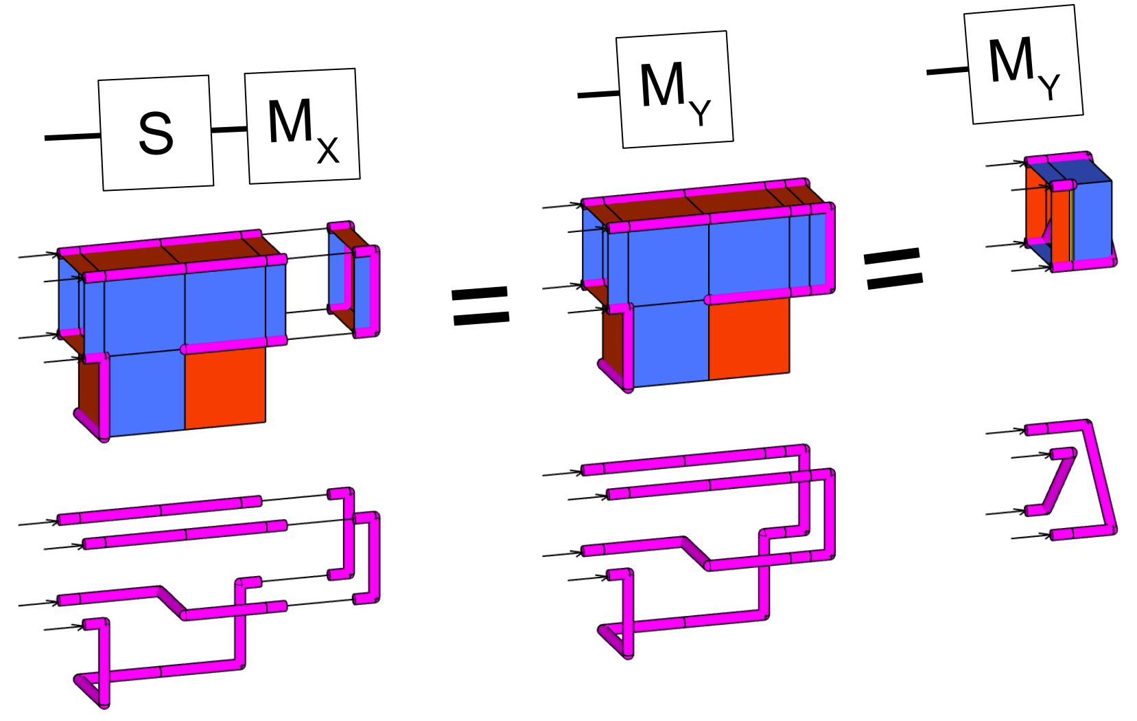
One way to find a topological implementation of an operation is to decompose it into operations whose topology you already know, connect them together, and deform the combined object to simplify it. Recall that a surface code patch has four twist defects, one at each corner [Bro+17] (see Appendix A for the definition of a twist defect). The Y basis measurement can be decomposed into an S gate followed by an X basis measurement. The S gate’s topology is to exchange the two twists at the ends of an X type boundary of the surface code patch [Bro+17]. The X basis measurement’s topology is to pair twists that share a Z type boundary, and then within each pair annihilate the twists by fusing them. The topological result of composing these two operations also fuses twist defects, but it pairs the twist defects across the diagonals of the patch. Thus, the topology of the Y basis measurement is to fuse twists diagonally (see Figure 2 and Figure 3).
In previous work, measuring a surface code qubit in the Y basis required increasing the size of the patch, in order to move twists without letting them get too close to each other [Bro+17, Bom+21, CC22]. My goal for this paper was to move the twists without resizing the patch. This requires the twists to travel diagonally across the patch, without compromising the code distance of the circuit.
The simplest circuit I found for moving a twist diagonally is summarized in Figure 4. However, although that circuit is simple, it isn’t efficient. After the twist moves through the diagonal, the surface code cycle has to wait while the data qubits are moved to close the gap created by the twist’s passage.
Finding a good circuit implementing the twist movement is difficult. The circuit has to measure all stabilizers of the input patch. The circuit has to change the boundary type of the patch. The circuit has to prepare all stabilizers of the output patch. The circuit has to orient and order operations carefully. As an example, note that the distance of the spacelike Y error (see Figure 6) is halved if two-qubit gates are pointed towards the crossing twist (instead of along it) during the middle two layers of the surface code cycle. The tactics I used to find satisfying circuits are summarized in Appendix C.
The best circuit that I found for moving a twist diagonally is summarized in Figure 5, and shown exactly in Figure 7. This circuit manages to merge all necessary qubit movement into a working surface code cycle, while using only one additional layer of entangling gates, and while preserving the full code distance. The idea that led to this circuit was to try running a normal surface code cycle in the bottom left of the patch while running a walking surface code cycle [MBG23] in the top right of the patch. I reasoned that the walking effect could be used to implement the domain wall defect that must be attached to the crossing twist, and that other details would follow as a consequence of this choice. Turning this idea into a complete circuit required finding a way to mesh the walking surface code cycle with the normal surface code cycle at the seam where they met, and finding a way to have the walking surface code switch the types of the boundaries of the patch instead of moving them.
Locally, the reason the circuit in Figure 7 works is because it is measuring all the stabilizers of the input surface code configuration and preparing all the stabilizers of the output surface code configuration. Globally, the reason this circuit works is because it changes the boundary types around the surface code patch from XZXZ to XXZZ. These local and global changes have the combined effect of fault tolerantly mapping the Y observable to a known product of stabilizers. A patch with XXZZ boundaries isn’t capable of storing a logical qubit. Instead, this patch has the property that, by multiplying all of the X basis stabilizers together, you can derive the value of a degenerate X observable running along the Z boundary. This product of stabilizers is what the Y observable is mapped to. By repeatedly measuring the stabilizers of the patch, you learn this product to arbitrarily high certainty [Gid22]. As will be shown in the next section, it’s sufficient to measure these stabilizers times. The measurement process is finished by destroying the patch by measuring all of its data qubits. To maximize code distance, each data qubit is measured in the basis of its closest boundary.
I verified the correctness of my construction in a variety of ways. First, locally, the key transition round is supposed to turn the Y observable into a product of measured stabilizers. The code I wrote declares that this transformation is supposed to occur during this part of the circuit, and locally verifies it using the same method that’s used to verify other stabilizer flows. Second, globally, a Y basis measurement should have the property that it correctly measures the value produced by a Y basis initialization. It’s tempting to simply time reverse the Y basis measurement to produce a corresponding initialization, but this wouldn’t detect mistakes such as accidentally measuring X instead of Y, so when verifying I used simple noiseless direct preparation of the observable and all stabilizers. I also verified against a magic state injection circuit set to inject the state. Third, if the construction is working, it’s supposed to have a code distance of . I checked the code distance using stim’s graphlike distance search and more general heuristic search. The shortest logical error found, within a patch under circuit noise, uses physical error mechanisms. The construction achieves the full code distance of the patch.


It’s notable that the timelike Y error mechanism shown in Figure 6 has distance , despite being caused by errors spanning across rounds and not spanning across space. This is because the relevant error mechanism requires a chain of X errors and a chain of Z errors crossing the rounds. Although there are error mechanisms that grow X and Z error chains together across space (e.g. Y basis data errors), there is apparently no corresponding mechanism that does this across time. A consequence of this asymmetry between space and time is that, unlike most surface code constructions, the Y basis measurement has a preferred spacetime orientation. Normally, performing a spacetime rotation of a defect diagram produces a different implementation of the same operation, with the same code distance. The Y basis measurement is different: a spacetime rotation of its defect diagram will turn the timelike Y error mechanism into a spacelike Y error mechanism that has half the distance. Avoiding this problem is why Figure 9 has two cases, one for spacelike motion and one for timelike motion.

3 Benchmarking
All circuits in this paper were simulated using the noise model defined in Appendix B. Decoding was done using an internal correlated minimum weight perfect matching decoder written by Austin Fowler. For each circuit, samples were taken until either a thousand logical errors had been seen or a billion shots had been taken, whichever came first. All simulated circuits were variations on memory experiments. The code, circuits, and statistics are available on Zenodo [Gid23].
In a memory experiment, a known logical state is initialized, protected against noise for some number of rounds, and then measured. The experiment succeeds if the measured state agrees with the prepared state, after error correction. Access to a Y basis measurement (and, by time reversal, a Y basis initialization), allows a Y basis memory experiment to be defined.
The Y basis memory experiment can be used to experimentally determine the optimal number of padding rounds to use for Y basis initialization and Y basis measurement. If not enough padding rounds are used, timelike error mechanisms become dominant and limit the fidelity. But the benefit of adding padding rounds saturates once these timelike error mechanisms have been suppressed below the noise floor set by spacelike error mechanisms. Figure 10 presents the results of simulations varying the number of padding rounds, showing that the benefit of adding padding rounds saturates at around rounds of padding.
An interesting property of the Y basis memory experiment is that preserving Y basis states (as opposed to X or Z basis states) better approximates the task of preserving the highly entangled states that would be present in a real quantum computation. Because X and Z type defects form large 2D surfaces in spacetime, while Y type defects only form narrow 1D curves, there are more places for X type errors and Z type errors to terminate and more paths they can follow. Thus, logical errors in the surface code are biased away from being Y type errors, making X and Z type errors the dominant logical error mechanisms. Y basis states and highly entangled states are sensitive to both of these dominant logical error mechanisms, while X and Z basis states are only sensitive to one. This difference is especially clear when focusing on stabilizer dependence. Although an X basis memory experiment measures both X type and Z type stabilizers, the logical value can be error corrected using only the measurement results from the X type stabilizers. Similarly, a Z basis memory experiment can be error corrected using only the measurement results from the Z type stabilizers. Protecting a Y basis state, or a highly entangled state, requires both the X stabilizer measurements and the Z stabilizer measurements. The Y basis memory experiment exercises the whole surface code, instead of only half.
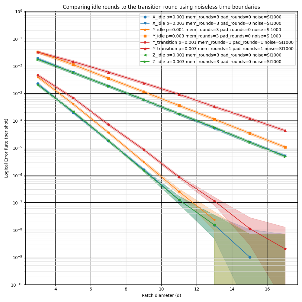
Because the Y basis memory experiment is sensitive to both X and Z logical errors, I expected Y basis memory experiments to have logical error rates roughly twice as high as X and Z memory experiments. However, simulations showed that the logical error rate was actually an additional 1.5 to 2.5 times higher than this expectation (see Figure 12). I was surprised by this difference, so I investigated where the additional error was coming from.
Because of Figure 10, I knew timelike errors weren’t the source of the problem. If they were, adding more padding would have fixed the issue. This left spacelike errors during the transition round as the likely cause. I checked this by isolating the transition round using magically noiseless time boundaries. (A magically noiseless time boundary performs perfect measurement of all stabilizers and observables of the code, preventing all error chains from crossing.) As controls, I also used magically noiseless time boundaries to isolate three rounds of idling in the X, Y, and Z bases. The results are shown in Figure 13. They suggest that the transition round is the source of the additional errors. (Also, they confirm Y basis idling is twice as hard as X or Z basis idling.)
Figure 11 digs further into the source of the extra errors by highlighting the paths that logical errors tend to follow during the transition round. It suggests that the problem is occurring along the path of the crossing twist. This makes sense to me, because the detectors along that path have the largest detecting regions (note where the biggest shapes are in Figure 7). This suggests that reducing the size of those detecting regions could bring the logical error rate in line with expectation. This is a place where there’s room for improvement in the circuit construction.
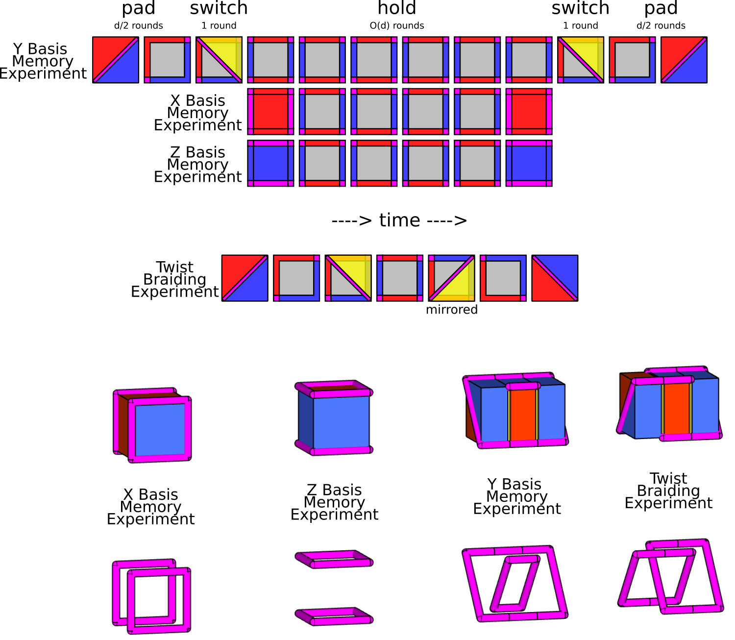
The last experiment that I simulated is an interesting variant of the Y basis memory experiment. In the normal Y basis memory experiment, which I’ll now start calling “the unlinked experiment" to avoid ambiguity, the initialization and measurement use the same orientation for the crossing twist. This produces a topology where the Y type defects form two unlinked rings in spacetime. In the other variant, which I’ll call “the braiding experiment", the initialization and measurement use opposite orientations, resulting in a topology where the Y type defects form linked rings (see Figure 15).
Figure 14 shows a key difference between the unlinked experiment and the braiding experiment. In the unlinked experiment, it’s always beneficial to reduce the time spent between the initialization and the measurement, whereas in the braiding experiment spending too few rounds idling increases the error rate dramatically. This is because, in the unlinked experiment, the twist crossing the patch during initialization is part of the same spacetime object as the twist crossing the patch during measurement. An error chain travelling from an object to itself has no effect on the state of the system (it is, effectively, a product of stabilizers). In the braiding experiment, the twist crossing the patch during initialization is part of a different spacetime object than the twist crossing the patch during measurement. It’s a logical error for error chains to travel between these two objects, and if there are too few idling rounds separating the objects then this error mechanism begins to dominate.
The braiding experiment highlights a subtle caveat on my claim that it takes rounds to perform a Y basis measurement. There are situations where additional idling rounds are needed, before the measurement, in order to keep the crossing twist away from other twists. This context-dependent-cost phenomenon isn’t unique to Y basis measurements. For example, the spacetime volume of a CNOT operation is reported based on a specific starting orientation of the involved qubits [Hor+12]. Other orientations require more volume. The sheer variety of possible contexts, and in particular the complex interdependence between how qubits are routed and oriented and operated upon, mean that describing the cost of a single operation using a single number is unavoidably an approximation. Ultimately, there are situations where the marginal cost of a Y basis measurement is in fact rounds and, based on my anecdotal experience assembling large surface code computations, I expect that these situations will be by far the most common. Therefore, despite the inherent ambiguity, I think rounds is the most appropriate number to use to describe the time it takes to perform the Y basis measurement presented in this paper.



4 Conclusion
In this paper, I presented a way to perform Y basis measurement and Y basis initialization in rounds, without leaving the bounding box of the surface code patch and while achieving full code distance. The spacetime volume of this construction is nearly an order of magnitude lower than achieved in previous work. I benchmarked the performance of this construction, and found that in short memory experiments it produces logical error rates slightly higher than would be expected given the performance of X and Z basis memory experiments, but good enough for practical use.
Having a faster Y basis measurement allows other computational primitives to be improved. For example, Figure 9 has concept diagrams for performing S gates by gate teleportation using the new Y basis measurement. These S gates use less spacetime volume than previous work. Faster Y basis measurement is also useful in the construction of magic state factories. For example, the magic state factories in [FG18, GF19] end with a layer of potential Y basis measurements. These measurements can now be performed faster than previously thought, increasing the expected execution speeds of those factories by around 10%.
The fact that the Y basis measurement can be performed inplace unlocks the ability to do tomography on hardware only large enough to store a single logical qubit. For example, suppose you’re interested in experimentally validating the fidelity of state injection. If only X and Z basis measurement are available, it’s impossible to distinguish between and , or between and a partially dephased state, because all these states have the same projection onto the XZ plane of the Bloch sphere. Adding the ability to do Y basis measurement makes these states distinguishable.
Looking beyond the Y basis, I’m hopeful there are other uses for the ability to move a twist diagonally across a surface code patch. More generally, I look forward to the discovery of more ways to lay defects across space and time, in ever more complex computational dances.
5 Acknowledgements
I thank Cody Jones for discussions that seeded the ideas that eventually turned into the Y basis measurement presented in this paper. I thank Matt McEwen for extensive discussions on the construction, and for encouragement to continue improving upon earlier versions of the circuit. I thank Austin Fowler for writing the correlated minimum weight perfect matching decoder used by this paper. I thank Austin Fowler, Alexis Morvan, Mike Newman, and Kevin Satzinger for giving feedback that improved the paper. I thank Hartmut Neven for creating an environment where this research was possible.
References
- [AGP05] Panos Aliferis, Daniel Gottesman and John Preskill “Quantum accuracy threshold for concatenated distance-3 codes” In arXiv preprint quant-ph/0504218, 2005 DOI: 10.48550/arXiv.quant-ph/0504218
- [And+20] Christian Kraglund Andersen, Ants Remm, Stefania Lazar, Sebastian Krinner, Nathan Lacroix, Graham J. Norris, Mihai Gabureac, Christopher Eichler and Andreas Wallraff “Repeated quantum error detection in a surface code” In Nature Physics 16.8 Springer ScienceBusiness Media LLC, 2020, pp. 875–880 DOI: 10.1038/s41567-020-0920-y
- [Bom+21] Hector Bombin, Chris Dawson, Ryan V Mishmash, Naomi Nickerson, Fernando Pastawski and Sam Roberts “Logical blocks for fault-tolerant topological quantum computation” In arXiv preprint arXiv:2112.12160, 2021 DOI: 10.48550/arXiv.2112.12160
- [Bro+17] Benjamin J Brown, Katharina Laubscher, Markus S Kesselring and James R Wootton “Poking holes and cutting corners to achieve Clifford gates with the surface code” In Physical Review X 7.2 APS, 2017, pp. 021029
- [CC22] Christopher Chamberland and Earl T Campbell “Universal quantum computing with twist-free and temporally encoded lattice surgery” In PRX Quantum 3.1 APS, 2022, pp. 010331 DOI: 10.1103/PRXQuantum.3.010331
- [FD12] Austin G Fowler and Simon J Devitt “A bridge to lower overhead quantum computation” In arXiv preprint arXiv:1209.0510, 2012
- [FG18] Austin G Fowler and Craig Gidney “Low overhead quantum computation using lattice surgery” In arXiv preprint arXiv:1808.06709, 2018
- [Fow+12] A.. Fowler, M. Mariantoni, J.. Martinis and A.. Cleland “Surface codes: Towards practical large-scale quantum computation” arXiv:1208.0928 In Phys. Rev. A 86, 2012, pp. 032324 DOI: 10.1103/PhysRevA.86.032324
- [GC99] Daniel Gottesman and Isaac L Chuang “Demonstrating the viability of universal quantum computation using teleportation and single-qubit operations” In Nature 402.6760 Nature Publishing Group, 1999, pp. 390
- [GE21] Craig Gidney and Martin Ekerå “How to factor 2048 bit RSA integers in 8 hours using 20 million noisy qubits” In Quantum 5 Verein zur Förderung des Open Access Publizierens in den Quantenwissenschaften, 2021, pp. 433 DOI: 10.22331/q-2021-04-15-433
- [GF17] Craig Gidney and Austin Fowler “A slightly smaller surface code S gate” In arXiv preprint arXiv:1708.00054, 2017
- [GF19] Craig Gidney and Austin G Fowler “Efficient magic state factories with a catalyzed CCZ to 2T transformation” In Quantum 3 Verein zur Förderung des Open Access Publizierens in den Quantenwissenschaften, 2019, pp. 135 DOI: 10.22331/q-2019-04-30-135
- [Gid+21] Craig Gidney, Michael Newman, Austin Fowler and Michael Broughton “A fault-tolerant honeycomb memory” In Quantum 5 Verein zur Förderung des Open Access Publizierens in den Quantenwissenschaften, 2021, pp. 605 DOI: 10.22331/q-2021-12-20-605
- [Gid21] Craig Gidney “Stim: a fast stabilizer circuit simulator” In Quantum 5 Verein zur Förderung des Open Access Publizierens in den Quantenwissenschaften, 2021, pp. 497 DOI: 10.22331/q-2021-07-06-497
- [Gid22] Craig Gidney “Stability Experiments: The Overlooked Dual of Memory Experiments” In Quantum 6 Verein zur Forderung des Open Access Publizierens in den Quantenwissenschaften, 2022, pp. 786 DOI: 10.22331/q-2022-08-24-786
- [Gid23] Craig Gidney “Data for "Inplace Access to the Surface Code Y Basis"” In Zenodo Zenodo, 2023 DOI: 10.5281/zenodo.7487893
- [Hän+20] Thomas Häner, Samuel Jaques, Michael Naehrig, Martin Roetteler and Mathias Soeken “Improved quantum circuits for elliptic curve discrete logarithms” In Post-Quantum Cryptography: 11th International Conference, PQCrypto 2020, Paris, France, April 15–17, 2020, Proceedings 12100, 2020, pp. 425 Springer Nature DOI: 10.1007/978-3-030-44223-1_23
- [Hor+12] Clare Horsman, Austin G Fowler, Simon Devitt and Rodney Van Meter “Surface code quantum computing by lattice surgery” In New Journal of Physics 14.12 IOP Publishing, 2012, pp. 123011 DOI: 10.1088/1367-2630/14/12/123011
- [Lit18] Daniel Litinski “A game of surface codes: Large-scale quantum computing with lattice surgery” In arXiv preprint arXiv:1808.02892, 2018
- [MBG23] Matt McEwen, Dave Bacon and Craig Gidney “Relaxing Hardware Requirements for Surface Code Circuits using Time-dynamics” arXiv, 2023 DOI: 10.48550/ARXIV.2302.02192
- [Mou16] Jonathan E Moussa “Transversal Clifford gates on folded surface codes” In Physical Review A 94.4 APS, 2016, pp. 042316 DOI: 10.1103/PhysRevA.94.042316
- [Vic13] Brett Victor “Media for Thinking the Unthinkable” [Online; accessed 12-Dec-2022], 2013 URL: http://worrydream.com/#!/MediaForThinkingTheUnthinkable
- [Zal+21] Adam Jozef Zalcman, Alan Derk, Alan Ho, Alex Opremcak, Alexander Korotkov, Alexandre Bourassa, Andre Gregory Petukhov, Andreas Bengtsson, Andrew Dunsworth, Anthony Megrant, Austin Fowler, Bálint Pató, Benjamin Chiaro, Benjamin Villalonga, Brian Burkett, Brooks Riley Foxen, Catherine Erickson, Charles Neill, Chris Quintana, Cody Jones, Craig Michael Gidney, Daniel Eppens, Daniel Sank, Dave Landhuis, David A Buell, Doug Strain, Dvir Kafri, Edward Farhi, Eric Ostby, Erik Lucero, Evan Jeffrey, Fedor Kostritsa, Frank Carlton Arute, Hartmut Neven, Igor Aleiner, Jamie Yao, Jarrod Ryan McClean, Jeremy Patterson Hilton, Jimmy Chen, Jonathan Arthur Gross, Joseph Bardin, Josh Mutus, Juan Atalaya, Julian Kelly, Kevin Miao, Kevin Satzinger, Kostyantyn Kechedzhi, Kunal Arya, Marco Szalay, Marissa Giustina, Masoud Mohseni, Matt McEwen, Matt Trevithick, Matthew Neeley, Matthew P Harrigan, Michael Broughton, Michael Newman, Murphy Yuezhen Niu, Nicholas Bushnell, Nicholas Redd, Nicholas Rubin, Ofer Naaman, Orion Martin, Paul Victor Klimov, Pavel Laptev, Pedram Roushan, Ping Yeh, Rami Barends, Roberto Collins, Ryan Babbush, Sabrina Hong, Sean Demura, Sean Harrington, Seon Kim, Sergei Isakov, Sergio Boixo, Ted White, Thomas E O’Brien, Trent Huang, Trevor Mccourt, Vadim Smelyanskiy, Vladimir Shvarts, William Courtney, Wojtek Mruczkiewicz, Xiao Mi, Yu Chen and Zhang Jiang “Exponential suppression of bit or phase flip errors with repetitive quantum error correction” In Nature, 2021 DOI: 10.1038/s41586-021-03588-y
- [Zha+22] Youwei Zhao, Yangsen Ye, He-Liang Huang, Yiming Zhang, Dachao Wu, Huijie Guan, Qingling Zhu, Zuolin Wei, Tan He, Sirui Cao, Fusheng Chen, Tung-Hsun Chung, Hui Deng, Daojin Fan, Ming Gong, Cheng Guo, Shaojun Guo, Lianchen Han, Na Li, Shaowei Li, Yuan Li, Futian Liang, Jin Lin, Haoran Qian, Hao Rong, Hong Su, Lihua Sun, Shiyu Wang, Yulin Wu, Yu Xu, Chong Ying, Jiale Yu, Chen Zha, Kaili Zhang, Yong-Heng Huo, Chao-Yang Lu, Cheng-Zhi Peng, Xiaobo Zhu and Jian-Wei Pan “Realization of an Error-Correcting Surface Code with Superconducting Qubits” In Physical Review Letters 129.3 American Physical Society (APS), 2022 DOI: 10.1103/physrevlett.129.030501
Appendix A Surface Code Defects
| Defect Type | Name | Shape | Effect | In Diagrams |
|---|---|---|---|---|
| I | Bulk | 3D | Conserves X and Z detection event parity | Empty Space |
| X | X Boundary | 2D | Absorbs detection events | Red Walls |
| Z | Z Boundary | 2D | Absorbs detection events | Blue Walls |
| H | Domain Wall | 2D | Cross-links detection events across the wall | Transparent Yellow Walls |
| Y | Twist | 1D | Absorbs adjacent detection events | Magenta Cylinders |
Detection events in the surface code can be classified into two types (X and Z), based on whether they are associated with an X type or Z type stabilizer changing unexpectedly. In the bulk of a surface code circuit, all errors produce an even number of detection events of each type. In other words, the bulk of the surface code “conserves X parity" and “conserves Z parity". These two conservation properties are what define the bulk. Any circuit location where Pauli errors conserve X detection event parity and conserve Z detection event parity is part of the bulk, regardless of the specific implementation details of the circuit.
Defects are circuit locations where X parity conservation and/or Z parity conservation is broken, because errors can produce an odd number of X detection events and/or an odd number of Z detection events. Important types of defects are summarized in Table 1. Locations in the circuit where an odd number of X detection events can be produced by an error are “X type defects" or “X boundaries". Locations where an odd number of Z detection events can be produced by an error are “Z type defects" or “Z boundaries". Locations where an error can produce one X detection event paired with one Z detection event, breaking the individual X and Z parities but not necessarily the combined parity, are “H type defects" or “Y type defects".
The distinction between H type defects (“domain walls") and Y type defects (“twists") is whether or not it’s possible to use the defect to terminate a combined chain of X errors and Z errors arriving from the same direction. An H type defect can’t be used to terminate such a chain, because the relevant errors always place the relevant X/Z detection events on opposite sides of the wall. A Y type defect differs in that it can terminate such a chain. For example, when a domain wall ends in the bulk, it always ends on a Y type defect because at that location errors can push a detection event around the wall to annihilate against a detection event that crossed through the wall.
There are many different ways to implement defects. For example, in the unrotated surface code, a spatial X boundary is implemented by three body stabilizers whereas, in the rotated surface code, two body stabilizers are used. Another example: the bulk of the surface code can be implemented on a square grid or on a hex grid [MBG23]. At a low level, the specific implementation used is extremely important because it affects performance (e.g. it can change the threshold). At a high level, the different implementations of defects are interchangeable. The computation performed by a surface code circuit can be understood in terms of the layout and topology of its spacetime defects, without knowing exactly how the defects are implemented. Thus, surface code computations can be improved both macroscopically, by changing the arrangement of defects, and microscopically, by changing the implementation of defects.
Appendix B Noise Model
All circuits in this paper were simulated using the superconducting-inspired noise model defined in Table 3. In legends, this noise model is called “SI1000" (short for Superconducting Inspired with 1000 nanosecond cycle). To provide a reference for comparisons to other error models or to hardware, the detection event fraction of the model at various noise strengths is plotted in Figure 16.
| Noise channel | Probability distribution of effects |
|---|---|
| Ideal gate | Noisy gate |
|---|---|
| (any single qubit unitary, including idling) | |
| (Wait for or ) |

Appendix C Tactics for building complex QEC circuits
In the past, when I’ve built quantum error correction circuits, I’ve used a strategy based on writing code to produce the desired circuit and then verifying that the final circuit was correct (e.g. by using Stim [Gid21] to verify the circuit’s graphlike code distance is as expected). For the Y basis circuits presented in this paper, that approach didn’t work. There were two major obstacles. First, although I could see roughly what had to happen in the circuit, I found it very difficult to work out exactly what the circuit should look like along the twist and at the boundaries of the patch. Second, even once I knew what the circuit should look like, it was difficult to write correct code for producing the circuit due to there being so many opportunities for easy-to-make mistakes like off-by-one errors and sign errors. Because of the these two obstacles, I would often get stuck in loops of fixing a problem by introducing a different problem.
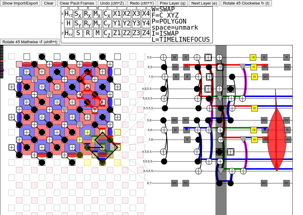
To make it easier to figure out what the circuit should look like, I wrote a stabilizer circuit editor with interactive automatic Pauli product propagation (see Figure 17). This was helpful for two reasons. First, tracking Pauli observables is a very common task when designing QEC circuits, but it’s slow and error-prone to do by hand. Computer software can do it billions of times faster, and more reliably. Second, manually editing the circuit is a much more direct form of interaction than iterating on code for producing a circuit [Vic13]. This completely nullifies whole classes of errors. For example, I make off-by-one errors when placing gates by math but I don’t make these errors when placing gates by hand. The key circuit cycle in Figure 7 was built, end to end, in this interactive editor before being translated into code.
To overcome the fact that each piece of the circuit was hard to get right, I switched from an integration testing paradigm to a unit testing paradigm. I focused on verifying that each individual surface code cycle was correct before attempting to combine it with the other cycles. Each cycle was still defined by a circuit, but now each cycle also had an accompanying list of required “stabilizer flows". A stabilizer flow has a desired starting stabilizer , an expected ending stabilizer , and a set of measurements to multiply into the stabilizer as it travels across the circuit. For example, if a cycle was supposed to measure a stabilizer using measurements and , then its list of stabilizer flows would contain . This allows each piece of the circuit to be independently verified because, given a circuit and a list of stabilizer flows, it’s possible to mechanically check whether or not the circuit has all the flows.
As a result of using this approach to piece verification, I found myself undergoing an interesting conceptual shift. I stopped thinking of surface code rounds as preserving stabilizers, and started thinking of them as recreating stabilizers. Instead of specifying and (translating to “ is preserved and is measured"), I found it more useful to specify and (translating to “ is measured and is prepared"). The benefit of this approach is that, when composing circuits, their flows can be matched together in order to form detectors. This turns annotating detectors, which I previously found to be one of the most error prone integration processes, into an automatic process.