A Provably Improved Algorithm for Crowdsourcing with Hard and Easy Tasks

Abstract

Crowdsourcing is a popular method used to estimate ground-truth labels by collecting noisy labels from workers. In this work, we are motivated by crowdsourcing applications where each worker can exhibit two levels of accuracy depending on a task’s type. Applying algorithms designed for the traditional Dawid-Skene model to such a scenario results in performance which is limited by the hard tasks. Therefore, we first extend the model to allow worker accuracy to vary depending on a task’s unknown type. Then we propose a spectral method to partition tasks by type. After separating tasks by type, any Dawid-Skene algorithm (i.e., any algorithm designed for the Dawid-Skene model) can be applied independently to each type to infer the truth values. We theoretically prove that when crowdsourced data contain tasks with varying levels of difficulty, our algorithm infers the true labels with higher accuracy than any Dawid-Skene algorithm. Experiments show that our method is effective in practical applications.

1 Introduction

Labeled datasets need to be collected to either train classifiers using supervised learning or evaluate their performance. To this end, crowdsourcing is often used to infer ground-truth labels after distributing tasks to workers and aggregating their responses. Participating workers may have distinct skill sets, and each worker can submit responses with different accuracies. To design and analyze the quality of inferred labels, a statistical model for the workers’ responses is often assumed.

A widely-studied model for crowdsourcing was first proposed by Dawid & Skene (1979). Their model assumes that the response of each worker $i$ to a task $j$ is correct with a fixed but unknown probability $p_{i}$. Although the true labels are never observed, it is possible to estimate the unknown accuracy parameters $p$ by assuming that workers respond according to this statistical model. The estimated accuracy parameters are then used to infer the truth values as the Nitzan-Paroush estimate (Nitzan & Paroush, 1983) or by iteratively applying the expectation maximization algorithm (Gao & Zhou, 2013). Despite the simplicity of this Dawid-Skene model, the optimal error rates of label estimation algorithms have only recently been understood (Berend & Kontorovich, 2014; Gao et al., 2016).

In this work, we are interested in modeling worker responses when crowdsourced tasks demand different levels of expertise. We model the response of workers by associating each task with one of two unknown types describing a task’s difficulty. In our model, each worker is assumed to correctly respond to a task depending on a reliability parameter determined by its type, and we characterize the difficulty of a task’s type as the mean-squared reliability of workers. Our model describes expert behavior in radiology when thoracic nodules have different shapes and sizes, or when they are imaged with lower resolutions, resulting in labels that are more reliable for one type of task than the other Shiraishi et al. (2000); He et al. (2016). Another application is to rank classifiers without accessing labeled data Parisi et al. (2014) that contain instances that are harder to classify than others.

Our contributions are as follows. We propose a new model for crowdsourcing that can describe how workers label tasks that require different levels of expertise. We then propose a spectral algorithm that clusters tasks into hard and easy types, and applies a Dawid-Skene algorithm for each of the types. We theoretically prove that our algorithm outperforms all Dawid-Skene algorithms; see Prop. 3.2 for a lower bound for Dawid-Skene algorithms and Thm. 3.4 for an upper bound for our algorithm. We conduct experiments based on real-world data to show the relevance of our method to practical applications.

2 Problem Setting and Related Work

Let $n$ be the number of workers labeling $d$ tasks, and denote $[n]=\left\{1,\dots,n\right\}$ to be the set of $n$ indices. Worker $i\in[n]$ submits a response $Y_{ij}\in\{-1,+1\}$ to task $j$ independently of other workers, and the goal is to estimate the truth value $y_{j}$ for every task $j\in[d]$. Each task $j$ is associated with a type $k_{j}\in\{1,2\}$, and the (unknown) reliability of workers determined by the task’s type as $r_{k_{j}i}=2{\mathbb{P}}(Y_{ij}=y_{j})-1$. The (one-coin) Dawid-Skene model is a special case when reliability vectors $r_{1}$ and $r_{2}$ are identical. For simplicity, we assume that the number of tasks $d_{k}$ per type $k$ is equal. Following prior work, we assume the truth values $y$ are drawn uniformly at random, and consider the regime $d>n\geq 3$ where a few workers label a large number of tasks.

Our hard-easy model is motivated by applications where certain tasks can inherently be more difficult than others. Precisely, we characterize the crowd’s potential for a type-$k$ task by the mean-squared reliability $\lVert r_{k}\rVert$ and assume the following condition between the two types.

Assumption 2.1.

There exists an “easy” and “hard” task type denoted as $k_{j}=1$ and $k_{j}=2$, respectively, where

$$\lVert r_{1}\rVert>\lVert r_{2}\rVert.$$ (1)

Note that our indexing of easy and hard tasks as $k_{j}=1$ and $k_{j}=2$ is without loss of generality, and is not known by the algorithm.

Crowdsourcing models differ in the structure assumed for the accuracy matrix $P$ with entries $P_{ij}={\mathbb{P}}(Y_{ij}=y_{j})$. A rank-1 model studied in Khetan & Oh (2016) incorporates task difficulty by restricting $P$ to be the outer product between workers’ accuracy and the task parameter vector. This is different from our problem setting where the accuracy matrix is generally not rank-1. A strict, non-parametric generalization was studied in Shah et al. (2021), where $P$ is assumed to satisfy strong stochastic transitivity Shah et al. (2016). In the context of crowdsourcing, this assumes that workers can be ranked from most to least accurate, and that this ranking does not change throughout tasks. In contrast, our model encompasses settings where the ranking of workers are arbitrarily different for the two types. Lastly, Shah & Lee (2018); Kim et al. (2022) analyzed a model where $P$ exhibits a low-rank structure with a fixed number of distinct entries. However, the number of distinct entries is not allowed to scale with the number of workers unlike the Dawid-Skene model where none of the workers may have identical reliabilities.

Note that, in our model, we assume all workers provide a label to all tasks. This is motivated by medical applications in which a company may contract with health-care professionals to label a large data set. It does not model applications such as Mechanical Turk in which workers independently select a sparse subset of tasks to label. Our model can be extended to accommodate such a sparsity in the data set, it would have the effect of having the sparsity parameter in the performance bounds. But given our motivation, we have chosen not to do so in this paper.

3 Main Results

3.1 Inadequacy of Universal Weighted Majority Votes

Assuming worker responses $Y$ are drawn according to a single reliability parameter $r\in[-1,+1]^{n}$, many Dawid-Skene algorithms estimate the reliability parameter as $\hat{r}\in(-1,+1)^{n}$ and use the Nitzan-Paroush estimate (Nitzan & Paroush, 1983) to estimate the true labels as

$$\hat{y}_{j}^{NP}=\text{sign}\left(\sum_{i}Y_{ij}\log\left(\frac{1+\hat{r}_{i}}{1-\hat{r}_{i}}\right)\right),$$ (2)

which is a weighted majority vote $\hat{y}_{j}^{WMV}=\text{sign}\left(\sum_{i}w_{i}Y_{ij}\right)$ with weights $w_{i}=\log\left(\frac{1+\hat{r}_{i}}{1-\hat{r}_{i}}\right)$. To analyze the above estimator, it is common to assume that the reliabilities lie in the interior of $(-1,1)^{n}$. We also assume this condition, where for each type $k$, there exists some $\rho_{k}\in(0,1/2)$ such that $\rho_{k}\leq\frac{1+r_{ki}}{2}\leq 1-\rho_{k}$ for every $i$. Furthermore, we denote $\rho_{0}=\min_{k}\rho_{k}$ to be the lower bound on $\rho_{k}$ over types $k$. In the aforementioned applications where tasks can be associated with different reliabilities, it is important to use different weights for each task type as shown next.

Here we state the error rate of all universal weighted majority votes, which uses a single weight vector and ignores the task’s type. For the following presentation, denote the average error rate as

$$P_{e}(w)=\lim_{d\to\infty}\frac{1}{d}\sum_{j}{\mathbb{P}}\left(\hat{y}_{j}^{WMV}\neq y_{j}\right).$$ (3)

Proposition 3.1.

Suppose $Y$ is drawn from the two-type Dawid-Skene model with reliability vectors $r_{1}$ and $r_{2}$. Then, the error rate of weighted majority vote with weights $w\in\mathbb{R}^{n}$ satisfies

$$-\log P_{e}(w)\geq n\min_{k}\varphi(w,r_{k}),$$

where $\varphi(w,r_{k})$ is defined as

$$-\min_{t>0}\frac{1}{n}\sum_{i=1}^{n}\log\left(\frac{1}{2}e^{tw_{i}}(1-r_{ki})+\frac{1}{2}e^{-tw_{i}}(1+r_{ki})\right)$$ (4)

Consider the universal weighted majority vote that minimizes the above label estimation error, i.e.

$$w^{*}=\arg\max_{w}\min_{k}\varphi(w,r_{k}).$$

With a slight abuse of notation, denote $\varphi(r_{1},r_{2})$ to be $\varphi(w,r_{k})$ with weights $w=\log\frac{1+r_{k^{\prime}}}{1-r_{k^{\prime}}}$. This corresponds to the error rate of a mis-specified Nitzan Paroush estimate, i.e. when estimating labels for one task type with weights corresponding to another type’s reliability. Next we state the best possible error rate achievable by a universal weighted majority vote using the above weights. This is strong in the sense that the lower bound holds for an estimate that has access to the true reliabilities $r_{1}$ and $r_{2}$.

Proposition 3.2.

Suppose $Y$ is drawn from the two-type Dawid-Skene model with reliability vectors $r_{1}$ and $r_{2}$ that both satisfy $\rho_{0}\leq\frac{1+r_{ki}}{2}\leq 1-\rho_{0}$ for all workers $i$. If $\left|\log\rho_{0}\right|=o(\sqrt{n}\varphi(r_{1},r_{2}))$, then as $n\to\infty$,

$$-\log P_{e}(w^{*})\leq\min_{k}(1+o(1))n\varphi(w^{*},r_{k})$$ (5)

In the following sections, we propose an algorithm that achieves improved error rates over any Dawid-Skene algorithm.

3.2 Method

We propose a spectral algorithm that clusters tasks into hard and easy types. Our algorithm constructs a task-similarity matrix and separates tasks based on the entries of its first eigenvector using a data-dependent threshold. Clustering algorithms can only estimate memberships up to a permutation, so we present clustering errors assuming the best permutation.

Algorithm 1 Clustering tasks into easy and hard types

  Input: observation matrix $Y\in\{-1,+1\}^{n\times d}$.

  Compute task-similarity matrix $T:=\frac{1}{n}Y^{T}Y$.

  Compute the principal eigenvector $v=v(T)$ of $T$.

  Compute threshold $\hat{\mu}=\frac{1}{d}\sum_{j}\left|\hat{v}_{j}\right|$.

  Classify task types by thresholding:

$$\hat{k}_{j}=\begin{cases}1&\text{if }v_{j}\in\left(-\hat{\mu},\hat{\mu}\right)\\ 2&\text{if }\left|v_{j}\right|>\hat{\mu}\\ U_{j}&\text{else}\end{cases},$$

where $U_{j}$ is drawn uniformly at random from $\{1,2\}$.

  Return: task type estimates $\hat{k}$.

Our algorithm used to clusters tasks by types is presented in Algorithm 1. Define a reliability matrix

$$R=\begin{pmatrix}\lVert r_{1}\rVert^{2}1_{d_{1}\times d_{1}}&r_{1}^{T}r_{2}1_{d_{1}\times d_{2}}\\ r_{1}^{T}r_{2}1_{d_{2}\times d_{1}}&\lVert r_{2}\rVert^{2}1_{d_{2}\times d_{2}},\end{pmatrix}$$ (6)

and let $\text{diag}(x)$ be the matrix with vector $x$ as its diagonal elements and zeros otherwise. The main idea behind Algorithm 1 was inspired by observing that the expected task-similarity matrix with entries

$${\mathbb{E}}T_{jl}=\frac{1}{n}{\mathbb{E}}\sum_{i}Y_{ij}Y_{il}$$ (7)

can be decomposed as

$$\frac{1}{n}R\otimes yy^{T}-\frac{1}{n}\text{diag}\left([\lVert r_{1}\rVert^{2}1_{d_{1}},\lVert r_{2}\rVert^{2}1_{d_{2}}]\right)+\text{diag}\left(1_{d}\right)$$

when the tasks are re-arranged so that type-1 tasks are on the first $d_{1}$ columns of the response matrix $Y$ and type-2 tasks on the remaining columns. Although this re-arrangement is unknown, the spectral properties of ${\mathbb{E}}T$ are invariant under column permutation, and our spectral algorithm can be analyzed assuming the above form.

The dominant eigen-pairs of the observed task-similarity matrix $T=\frac{1}{n}Y^{T}Y$ concentrates around those of ${\mathbb{E}}T$ with more workers $n$, whose spectral properties are in turn dominated by $R$ as the number of tasks $d$ grows large. Because our algorithm uses the principal eigenvector of $T$ to assign cluster memberships, it is convenient to define a quantity that determines the gap between its entries. Define the quantity

$$\omega=\left|\frac{\lVert r_{1}\rVert^{2}-\lVert r_{2}\rVert^{2}}{2r_{1}^{T}r_{2}}\right|>0$$ (8)

which increases with a larger gap $\lVert r_{1}\rVert^{2}-\lVert r_{2}\rVert^{2}$ between crowd potentials of type 1 and 2 tasks, or as the angle between reliabilities $r_{1}$ and $r_{2}$ increases. The square of difference between the largest two eigenvalues $\lambda_{1}$ and $\lambda_{2}$ of $R$ is scaled to define the positive quantity

$$\Delta^{2}=\frac{4}{d^{2}n^{2}}\left(\lambda_{1}-\lambda_{2}\right)^{2}.$$ (9)

Entries of the principal eigenvector $v$ of the reliability matrix $R$ take up to four distinct values $\pm e_{1}$ and $\pm e_{2}$, whose ratio is given by

$$\gamma\overset{\Delta}{=}\left|\frac{e_{1}}{e_{2}}\right|=\omega+\sqrt{\omega^{2}+1}.$$ (10)

We adopt the convention that eigenvectors are unit-norm, in which case the difference between the positive entries $e_{1}$ and $e_{2}$ is

$$(e_{1}-e_{2})^{2}=\frac{(\gamma-1)^{2}}{\gamma^{2}+1}\frac{2}{d}.$$ (11)

Unlike more common applications of spectral clustering Von Luxburg (2007), crowdsourcing involves unknown binary labels $y$ that affect the sign of $\hat{v}$. If the number of workers is sufficiently large, we can use the sign of $\hat{v}$ to estimate the true labels $y$ without separating tasks by type as done similarly by Dalvi et al. (2013). However, the error rate of estimating $y$ as the sign of $\hat{v}$ is dominated by $1/e_{2}$, where $e_{2}$ is the entry in the expected eigenvector $v$ corresponding to hard tasks. The magnitude of $e_{2}$ is small when there is a large eigen-gap $\gamma$, and the number of workers required to estimate $y$ as the sign of $\hat{v}$ can be much larger than the mild $n=\Omega\left(\log d\right)$ requirement for statistically-efficient Dawid-Skene algorithms Zhang et al. (2016).

Instead of using the sign of $\hat{v}$ to directly estimate truth values whose error rate is dominated by $e_{2}$, our algorithm uses the observation that the threshold rule

$$\hat{k}_{j}=\begin{cases}1:\left|\hat{v}_{j}\right|>\hat{\mu}\\ 2:\left|\hat{v}_{j}\right|<\hat{\mu}\end{cases}$$

where $\hat{\mu}=\frac{1}{d}\sum_{j}\left|\hat{v}_{j}\right|$ is the average of magnitudes in the principal vector $\left|\hat{v}\right|$, depends on the eigen-gap $\gamma$ which is large when $r_{1}^{T}r_{2}$ is small or the $\lVert r_{1}\rVert^{2}-\lVert r_{2}\rVert^{2}$ is large. The average magnitude $\hat{\mu}$ of entries quickly converges to the average $\mu=\frac{1}{d}\sum_{j}\left|v_{j}\right|$ corresponding to the principal eigenvector $v$ of the reliability matrix $R$. Combining the above observations, we were able to prove that Algorithm 1 can cluster tasks with the mild condition that the number of workers grows with $\log d$.

Theorem 3.3.

If the number of workers satisfies

$$n=\Omega\left(\frac{\gamma^{2}+1}{(\gamma-1)^{2}}\frac{\log d}{\Delta}\right),$$ (12)

Algorithm 1 returns cluster memberships $\hat{k}$ such that with probability $\geq 1-1/d$,

$$\frac{1}{d}\sum_{j}\mathbf{1}\{\hat{k}_{j}\neq k_{j}\}\leq A\frac{1}{n}\frac{\gamma^{2}+1}{(\gamma-1)^{2}}\frac{\log d}{\Delta}$$ (13)

for some universal constant $A>0$.

As the ratio $\gamma$ or eigen-gap $\Delta$ grows, Algorithm 1 requires fewer workers and its clustering error is reduced. We simulate the easy-hard model for various values of $r_{1},r_{2}$ and show in Figure 1 that the analysis is tight with respect to $\gamma$ and $\Delta$.

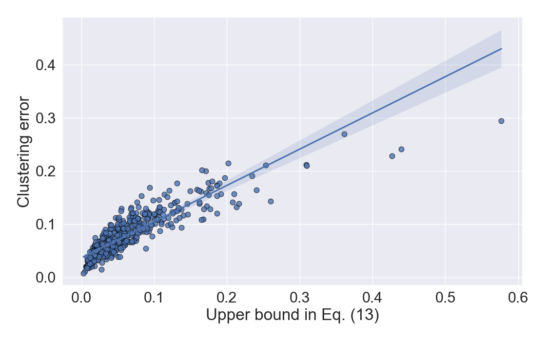
Figure 1: A line of best fit comparing Monte Carlo simulations of the clustering error $(n=50,d=200)$ with our error bound in Eq. (13), adjusted by a constant multiplicative factor, demonstrates that our theoretical analysis is tight in $\gamma$ and $\Delta$.

When the difference of reliability norms $\lVert r_{1}\rVert^{2}-\lVert r_{2}\rVert^{2}$ is small or the inner product $r_{1}^{T}r_{2}$ is large, the above bound suggests an impossibility result that tasks cannot be clustered by type. Inspecting Eq. (12), this occurs when

$$\sum_{j}(\left|\hat{v}_{j}\right|-\hat{\mu})^{2}\approx\frac{1}{2}\frac{(\gamma-1)^{2}}{\gamma^{2}+1}<A^{\prime}\frac{1}{n}\frac{\log d}{\Delta}$$ (14)

is satisfied for some universal constant $A^{\prime}>0$. Estimating $\Delta$ in Eq. (9) through the eigen-values of the task-similarity matrix $T$ as $\hat{\Delta}=\hat{\lambda}_{1}-\hat{\lambda}_{2}$, we have a data-driven estimate of when tasks cannot be clustered as

$$\left(\hat{\lambda}_{1}-\hat{\lambda}_{2}\right)\sum_{j}(\left|\hat{v}_{j}\right|-\hat{\mu})^{2}<A^{\prime}\frac{1}{n}\log d.$$ (15)

From this observation, we suggest to first numerically verify the condition in Eq. (15) and only cluster tasks using Algorithm 1 when the reversed inequality is satisfied.

3.3 Label Estimation Error

Any Dawid-Skene algorithm can be used to infer the truth values separately for each task type. Our goal in this section is to prove that at least one Dawid-Skene algorithm can still correctly infer the true labels even though a small fraction of tasks may be incorrectly clustered by Algorithm 1. Here we focus on the Triangular Estimation (TE) algorithm proposed by Bonald & Combes (2017) because it is one of the more recent algorithms with strong guarantees for the Dawid-Skene model.

Let

$$\mathcal{J}_{k}=\left\{j:\hat{k}_{j}=k\right\}$$ (16)

be the set of tasks that are assigned cluster membership $k$. In our setting, the TE algorithm is applied to type-$k$ tasks by constructing a worker-covariance matrix

$$\hat{C}_{ab}=\frac{1}{\left|\mathcal{J}_{k}\right|}\sum_{j\in\mathcal{J}_{k}}Y_{aj}Y_{bj}$$ (17)

for each worker-pair $(a,b)$. For every worker $i$, the most informative co-workers $a_{i},b_{i}=\arg\max_{a\neq b\neq i}\left|\hat{C}_{ab}\right|$ are computed, and the magnitude of worker $i$’s reliability is estimated as

$$\left|\hat{r}_{ki}\right|=\sqrt{\left|\frac{\hat{C}_{a_{i}i}\hat{C}_{b_{i}i}}{\hat{C}_{a_{i}b_{c}}}\right|}\mathbf{1}\left\{\hat{C}_{a_{i}b_{i}}>0\right\}.$$ (18)

The sign of workers is estimated by determining the worker $i^{*}$ whose covariance estimate is obtained with the highest confidence bound, then assigning the sign of other workers’ reliabilities by referencing this worker’s reliability estimate.

To analyze the TE algorithm, we define some additional problem parameters following (Bonald & Combes, 2017). The quantity $V_{k}=\min_{i}\max_{a\neq b\neq i}\sqrt{\left|r_{ka}r_{kb}\right|}$ measures a lower bound on how informative workers’ responses are. To ensure that the parameters $r$ are identifiable, we assume that both $V_{k}$ and the average reliability $\bar{r}_{k}=\frac{1}{n}\sum_{i}r_{ki}$ are positive.

The idea behind our result is that estimating the reliabilities $r$ is still possible although a small fraction of the tasks are incorrectly classified. We show that as long as the fraction of relevant tasks $\left(Y_{ij}:j\in\mathcal{J}_{k},k_{j}=k\right)$ is sufficiently large, the TE algorithm is still able to estimate reliabilities with high confidence in the presence of noise resulting from imperfect clustering.

Algorithm 2 Crowdsourcing with hard and easy tasks

  Input: observation matrix $Y\in\{-1,+1\}^{n\times d}$ and a partition of $n$ workers $\mathcal{N}_{1},\mathcal{N}_{2}$.

  Use the first set of workers $\mathcal{N}_{1}$ to separate $d$ tasks into easy and hard clusters $\mathcal{J}_{1},\mathcal{J}_{2}$ using Algorithm 1.

  for each type $k\in\{1,2\}$ do

     Use the second set of workers $\mathcal{N}_{2}$ to estimate true labels $\hat{y}_{j}$ for tasks $j\in\mathcal{J}_{k}$ with a Dawid-Skene algorithm.

  end for

The optimal error rate (Gao et al., 2016) that can be achieved for any given type $k$ is determined by the order-$1/2$ Renyi-divergence from $\frac{1-r_{ki}}{2}$ to $\frac{1+r_{ki}}{2}$, defined below.

$$\Phi_{k}:=\frac{1}{2}\sum_{i}\log\left(1-r_{ki}^{2}\right)$$ (19)

We next show that clustering tasks before applying the TE algorithm can significantly improve the label estimation error if the clustering error does not exceed a multiple of $\frac{\Phi_{k}}{\log n}$ or the average reliability for both types $k$. For simplicity of presentation, assume $\bar{r}_{k}\geq\frac{3}{n}$.

Theorem 3.4.

Let

$$\eta_{k}=\frac{\left|\{j\in\mathcal{J}_{k}:k_{j}\neq k\}\right|}{\left|\mathcal{J}_{k}\right|}$$ (20)

be the fraction of tasks included in $\mathcal{J}_{k}$ but drawn according to $r_{k^{\prime}}$, where $k^{\prime}\neq k$. If the fraction of incorrectly clustered tasks satisfies

$$\eta_{k}\leq\frac{V_{k}}{48}\min\left\{\frac{\Phi_{k}}{\log n}V_{k}\rho_{k},3\bar{r}_{k}\right\}$$ (21)

and the number of tasks used to estimate type-$k$ labels is

$$\left|\mathcal{J}_{k}\right|=\Omega\left(\frac{\log n^{2}\left|\mathcal{J}_{k}\right|}{V^{2}\min\left\{V^{2}\Phi_{k}^{2}\rho_{k}^{2},n\bar{r}_{k}^{2}\right\}},\right),$$

then as $n,\left|\mathcal{J}_{k}\right|\to\infty$,

$${\mathbb{P}}\left(\hat{y}_{j}\neq y_{j}|k_{j}=k\right)\leq\exp\left(-(1+o(1))n\Phi_{k}\right).$$ (22)

For comparison, the label estimation error for the universal weighted majority vote in Eq. (5) can be much larger than above, as seen through the inequality

$$\varphi(w,r_{k})\leq\Phi_{k},$$ (23)

with equality if and only if the maximum likelihood weights $w=\log\frac{1+r_{k}}{1-r_{k}}$ are used. Therefore, our algorithm strictly outperforms all universal weighted majority votes on crowdsourced data containing easy and hard tasks whenever $n$ is sufficiently large.

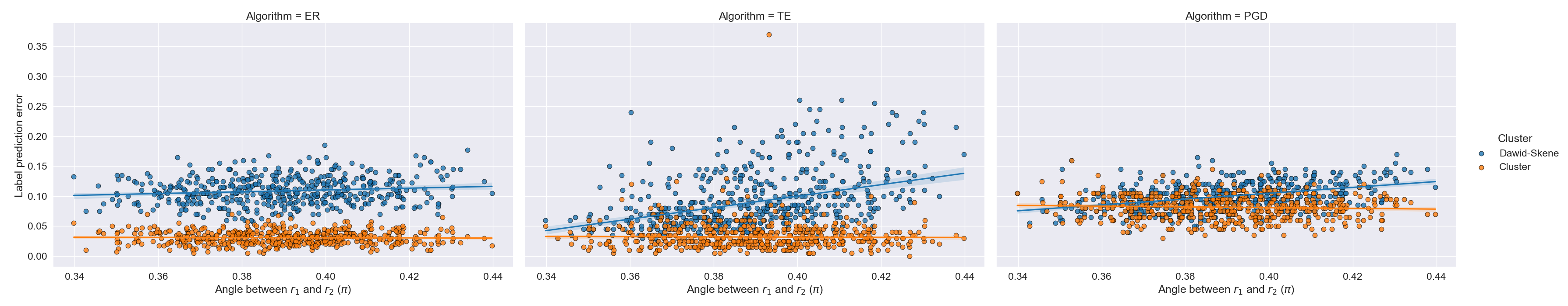
Figure 2: Transition from Dawid-Skene to a Two-Type Model as the angle between $r_{1}$ and $r_{2}$ increases.

3.4 Overall Algorithm

The overall procedure of estimating truth labels $y$ is presented in Algorithm 2. The algorithm first randomly splits the $n$ workers into two disjoint subsets $\mathcal{N}_{1}$ and $\mathcal{N}_{2}$ for the technical reason that re-using the same observations $Y$ for both clustering and label estimation steps violates independence assumptions. However in practice, we use all $n$ workers for both the clustering and label estimation steps.

If we select workers $\mathcal{N}_{1}$ so that $n_{1}=\left|\mathcal{N}_{1}\right|$ satisfies Eq. (12) to cluster tasks, Algorithm 1 returns cluster membership sets

$$\mathcal{J}_{k}=\left\{j\in[d]:\hat{k}_{j}=k\right\},k\in\{1,2\}$$ (24)

which satisfy

$$\eta_{k}\leq C\left(\frac{1}{n_{1}}\frac{\gamma_{1}^{2}+1}{(\gamma_{1}-1)^{2}}\frac{\log d}{\Delta_{1}}\right)$$ (25)

with high probability for both $k\in\{1,2\}$ and some constant $C>0$, where the $\gamma_{1}$ and $\Delta_{1}$ are problem-parameters relevant to workers $\mathcal{N}_{1}$. Running the TE algorithm on tasks $\mathcal{J}_{1}$ and $\mathcal{J}_{2}$ separately guarantees that the error rate satisfies Eq. (22), where the problem parameters depend on workers $\mathcal{N}_{2}$. Combining, we have the following result.

Theorem 3.5.

Suppose that for each task type $k$, the $n_{1}$ workers $\mathcal{N}_{1}$ used to cluster tasks satisfy

$$n_{1}\geq\frac{\gamma^{2}+1}{(\gamma-1)^{2}}\frac{\log d}{\Delta}\max\left\{\frac{48\log n_{1}}{V_{k}^{2}\Phi_{k}\rho_{k}},3\bar{r}_{k}\right\}.$$ (26)

with respective problem parameters $\gamma,\Delta$. Then, all of the following hold with high probability as $n_{2},\left|\mathcal{J}_{k}\right|\to\infty$.

$${\mathbb{P}}\left(\hat{y}_{j}\neq y_{j}|\hat{k}_{j}=k_{j}\right)\leq\exp\left(-(1+o(1))n_{2}\Phi_{k_{j}})\right),$$

$${\mathbb{P}}\left(\hat{y}_{j}\neq y_{j}|\hat{k}_{j}\neq k_{j}\right)\leq\exp\left(-(1+o(1))n_{2}\varphi(r_{1},r_{2})\right).$$

Lastly, we describe how to detect the presence of easy-hard tasks or multiple levels of difficulty. When there are enough tasks, the eigen-spectrum of the same task-similarity matrix contains $K$ dominant eigenvalues, and the remaining $d-K$ eigenvalues do not grow with the number of tasks $d$. Therefore, the number of difficulty levels can be estimated as the number of dominant eigenvalues by inspecting the eigenspectrum of the task similarity matrix. Other methods that can be used to detect the number of task types include parallel analysis (Dinno, 2009) or improved methods (Dobriban & Owen, 2018). Regardless of whether there are two or more levels of difficulty, our clustering method is expected to consistently enhance the performance of Dawid-Skene methods when the reliability vectors sufficiently differ.

4 Experiments

Transition from Dawid-Skene to Two-Type Model: As our theoretical analyses suggest, there is a transition from Dawid-Skene algorithms performing well to their requiring a clustering step due to the variation of reliability across task types. We perform numerical simulations to empirically identify this phase transition in Figure 2. The reliabilities were set so that distinct entries in the reliability vectors remain the same and label estimation performance is affected only by the angle between $r_{1}$ and $r_{2}$. The squared norm difference is set as $\lVert r_{1}\rVert^{2}-\lVert r_{2}\rVert^{2}\approx 13$. As shown, the label prediction error increases for Dawid-Skene algorithms whereas clustering remains nearly constant throughout all angles $\in(0,\pi)$. Furthermore, ER and TE both under-perform their clustered counterparts even for small angles, and PGD benefits from clustering for most angles.

Baseline Algorithms: First, we report the performance of the following Dawid-Skene algorithms: unweighted majority vote (MV), ratio of eigenvectors (ER, Dalvi et al. 2013), TE (Bonald & Combes, 2017), and Plug-in gradient descent (PGD, Ma et al. 2022). Then we compare their label estimation errors when applied separately after clustering using our Algorithm to demonstrate the importance of separating tasks by type. A very large number of algorithms have been proposed for crowd sourcing including Spectral-EM (Zhang et al., 2016), OBI-WAN (Shah et al., 2021), message-passing algorithms (Karger et al., 2014; Khetan & Oh, 2016) to name just a few. So it is difficult to perform a comparison with all existing algorithms. We have chosen to compare our algorithms to Dalvi et al. (2013); Bonald & Combes (2017); Ma et al. (2022) for the following reasons:

• As mentioned in our theoretical analysis, applying the algorithm in Dalvi et al. (2013) would result in the performance being dominated by the hard tasks while that is not the case with our algorithm. We wanted to demonstrate this phenomenon in the experiments. While this may also happen with other models, we were able to theoretically demonstrate it for the algorithm in Dalvi et al. (2013) and hence, we are doing an experimental comparison.

• The papers (Bonald & Combes, 2017; Ma et al., 2022) have already compared their algorithms to previous literature such as Zhang et al. (2016) and demonstrated that their algorithms perform better.

• The number of parameters in (Shah et al., 2021) is very large and as a result, the performance of their algorithm in the datasets that we have used is very poor. So we are not showing a comparison to the algorithm in Shah et al. (2021) in this paper.

Datasets: Our first experiment is based on how radiologists identify pneumonia from chest radiography. Chest radiography is used as an initial imaging test to identify pneumonia, followed by computational tomography (CT) when an abnormality is detected. For this experiment, we use the data reported in (Makhnevich et al., 2019) to explore how to form a consensus from radiologists in a multi-reader setting.

Table 1: JSRT dataset description. Size is in millimeters, and a subtlety of 0 indicates that a nodular pattern is absent.

Subtlety	0	1	2	3	4	5
Count	93	25	29	50	38	12
Size	0.0	23.0	17.9	17.2	16.4	14.6
Acc. (%)	80.9	99.6	92.6	75.7	54.7	29.6

Table 2: Summary statistics for datasets crowdsourced to non-experts, after processing. To compute $\omega$, we use the available ground-truth values to measure the accuracy of workers.

Dataset	# Workers	# Tasks	$\omega$
Blue Bird	39	108	64.3
Dog	78	807	31.5

The Japanese Society of Radiological Technology (JSRT) Database and its report (Shiraishi et al., 2000) was used, which contains the performance of 20 radiologists for identifying solitary pulmonary nodules in chest radiographs. Its dataset statistics are summarized in Table 1. Expert performances are reported for various levels of subtlety defined by the size of nodular patterns. It is clear that detecting nodular patterns becomes significantly more difficult as the size is decreased, demonstrating a multi-type phenomenon with varying levels of task difficulty.

We also experiment with other datasets used for crowdsourcing: Bluebird (Welinder et al., 2010), Dog (Deng et al., 2009), RTE (Snow et al., 2008), and Temp (Snow et al., 2008). These datasets contain simple tasks that were assigned to non-experts through online platforms. Dog contains 4 classes, and we convert this to two groups $\{0,2\}$ vs. $\{1,3\}$ and perform binary classification following Bonald & Combes (2017).

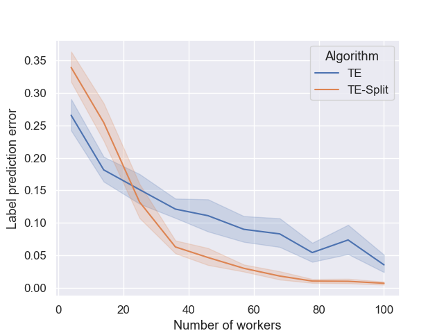
(a) Sensitivity and specificity used as accuracy.

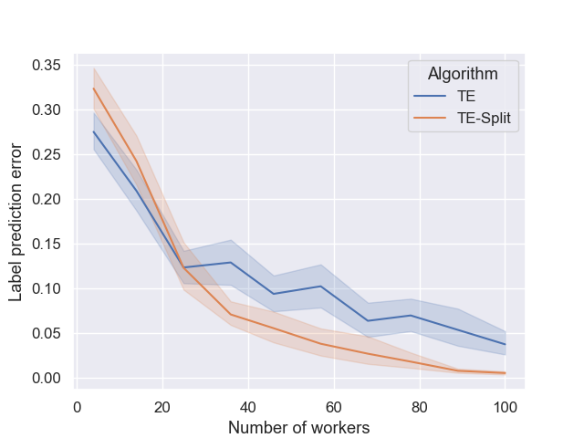
(b) Sensitivity and specificity used as TPR and TNR.

Figure 3: Pneumonia experiments: A comparison of TE with and without clustering. (a) interprets the reported sensitivity and specificity as worker accuracy; (b) uses sensitivity and specificity to define true positive (TPR) and true negative rates (TNR).

Setup: For the pneumonia datasets, we investigate the effect of clustering through two experiments. Both experiments use the reported ranges of sensitivity $[0.33,0.777]$ and specificity $[0.588,0.94]$ to generate worker reliability vectors as follows. Each worker’s accuracy is drawn uniformly at random from the reported minimum and maximum values. For the first experiment, half the tasks are assigned type-1 and the other type-2. The sensitivity and specificity are interpreted as accuracies for each type when generating the workers’ response. The second experiment uses sensitivity and specificity as true positive and true negative rates (TPR/TNR), meaning the probability of response being correct conditioned on the true class (positive or negative). Truth values are drawn uniformly at random for a count of $d=200$, and the plots are an average over $40$ trials.

Our setup for the JSRT experiments are as follows. There is a total of 6 types according to the specificity and sensitivity reported for 5 subtlety levels. These values are used as the accuracy for each type. JSRT-2 combines the higher and lower 3 accuracy parameters, and JSRT-6 uses all 6 types. Using their reported means and standard deviations $\{\bar{r}_{k}\}_{k},\{\sigma_{k}\}_{k}$, we sample $\frac{1+r_{ki}}{2}$ from the uniform distribution with support $\bar{r}_{k}\pm\sigma_{k}$. Each truth value $y_{j}$ is drawn randomly from its class-distribution defined by the sample mean of positive (presence of nodules) cases. We then sample the crowd’s response following the number of tasks per type in Table 1.

For the crowdsourcing datasets labeled by non-expert workers, we impute the no-response entries as follows. First, we follow (Bonald & Combes, 2017) and remove workers who respond to $\leq 10$ labels. Then using the true label values, we compute for each task the fraction of workers who correctly labeled a task divided by the number of workers who responded to the same task. After separating the tasks by rank in half, the empirical reliability of workers are computed for each type and the no-response entries are imputed with their corresponding reliability vectors. The problem parameter $\omega$ computed based on the empirical reliabilities suggests that the datasets contain tasks with different difficulties, and that the reliabilities of workers can vary significantly from one type to another. Note that this value is computed before imputation. Dataset statistics are shown in Table 2 after processing as above. RTE and Temp datasets contain extremely easy tasks, where when processed to be dense as above, majority vote and other algorithms achieve 100% accuracy. Therefore we do not report experiments on these datasets, as there is no room for improvement. All experiments report the average over 10 trials.

Table 3: Label estimation errors (%) for the JSRT experiments. “U” and “S” after dataset names indicate whether label estimation was performed without or with separation, respectively.

Dataset	MV	ER	TE	PGD
JSRT-2-U	5.65	5.65	4.74	5.06
JSRT-2-S	5.65	4.39	3.16	3.81
Gain	0.00	1.26	1.58	1.25
JSRT-6-U	10.30	10.30	9.96	9.72
JSRT-6-S	10.30	10.02	9.84	9.76
Gain	0.00	0.28	0.12	-0.04

Table 4: Label estimation errors (%) on datasets crowdsourced to non-experts.

Dataset	MV	ER	TE	PGD
Bird-U	24.07	28.70	17.59	25.00
Bird-S	24.07	11.11	12.96	19.44
Gain	0.00	16.59	4.63	5.56
Dog-U	23.28	23.32	35.38	20.06
Dog-S	23.28	7.11	14.40	21.72
Gain	0	16.21	20.98	1.66

Results: For pneumonia detection, we compare the performance of TE with and without our clustering algorithm in Figures 3 (a) and (b). Although requesting that each chest radiograph be inspected by a large number of radiologists would be excessively costly, the results reveal a few interesting observations.

Other crowdsourcing applications that use low-cost workers inevitably suffer from high variation in reliability Whitehill et al. (2009). When the task difficulty levels are diverse enough to cause workers to be more accurate for a subset of the tasks, clustering is shown to be effective. The number of workers at which clustering starts to enhance label prediction performance depends on the quantity $\omega$ in Eq. (37), which depends on how the accuracies of workers vary across tasks. Third, many datasets in medical imaging are constructed as a consensus of 3 or more experts Obuchowski & Zepp (1996); Ørting et al. (2020). These studies may benefit from our analysis by using data-driven techniques instead of a simple majority vote to determine ground-truth labels when the inter-reader agreement is low. Lastly, the performance curves are similar regardless of whether the sensitivity and specificity values are interpreted as class-independent or class-conditional accuracies. The latter is an analogue to the two-coin Dawid-Skene model. Our model is more general than the two-coin Dawid-Skene model when the class-conditional reliability parameters differ by a sufficient gap, as it is a special case that the task type is a one-to-one correspondence to the truth values.

The performance of crowdsourcing algorithms with and without our clustering algorithm is shown in Table 3 for the medical imaging dataset. As shown, separation consistently increases accuracy over Dawid-Skene algorithms. Because experts labeled the JSRT dataset, we observe a high accuracy using the simple majority vote. However, missing to identify nodules can be consequential and even a small gain in accuracy is critical.

Label estimation errors for datasets containing tasks that were labeled by non-expert workers through crowdsourcing platforms are shown in Table 4. Again we observe that clustering improves performance, and preserves the 100% accuracies on RTE and Temp datasets. In addition to the label estimation errors, we compute the data-dependent quantity in Eq. (15) which we re-arrange as

$$\frac{n(\hat{\lambda}_{1}-\hat{\lambda}_{2})}{\log d}\sum_{j}(\left|\hat{v}_{j}\right|-\hat{\mu})^{2}.$$ (27)

Recall that this is a data-dependent quantity which can be used to determine the separability between two types: a larger value predicts that the two reliability vectors differ more. Aligning with our analysis, this quantity is the smallest for the Bird dataset where we observe a smaller gain for performance on average than for Dog, for which we observe this quantity to be the highest of the four. Specifically, the ratio of this quantity evaluated on Dog to that on Bird is approximately $27$.

In general, we observe a smaller gain for the PGD algorithm. However on the non-expert crowdsourcing datasets, we observe that other Dawid-Skene algorithms applied to clustered tasks outperform PGD. We suspect that this is because while PGD is especially robust to various sparsity structures on the worker-task assignment graph (Ma et al., 2022), its benefits over other Dawid-Skene algorithms diminish for the dense observations we consider.

5 Conclusion

We proposed a crowdsourcing model which we show to be more appropriate than the Dawid-Skene model when there are tasks that require different levels of skill sets. Then we described a spectral clustering algorithm that clusters tasks by difficulty, and theoretically analyzed the statistical error of label estimation when using or without using a clustering step. Experiments confirm our theoretical findings and demonstrate the benefits brought by our modeling and algorithm.

Appendix A Detailed Expressions and Proofs

A.1 Upper bound for Universal Weighted Majority Vote

Recall the label estimation error $P_{e}(w)=\lim_{d\to\infty}\frac{1}{d}\sum_{j}{\mathbb{P}}\left(\hat{y}_{j}^{WMV}\neq y_{j}\right)$ defined in equation 3. We drop the task subscript and write $k_{j}=k$. For each worker $i$ and task $j$, define the signed indicator $G_{ij}$ to be the random variable that is $-1$ with probability $\frac{1}{2}(1-r_{ki})$ and $+1$ otherwise.

$$\mathbb{P}\left(\tilde{y}_{j}\neq y_{j}\right)=\mathbb{P}\left(\sum_{i=1}^{n}w_{i}G_{ij}<0\right)$$

For any $t>0$, we bound the error probability using Markov’s inequality on the moment generating function as

$$\mathbb{P}\left(\sum_{i=1}^{n}w_{i}G_{ij}>0\right)=\mathbb{P}\left(\exp\left(-t\sum_{i=1}^{n}w_{i}G_{ij}\right)>1\right)\leq\mathbb{E}\left(\exp\left(-t\sum_{i=1}^{n}w_{i}G_{ij}\right)\right)$$ (28)

Because workers respond independently of each other, $G_{1j},\dots,G_{nj}$ are mutually independent and

$$\mathbb{E}\left(\exp\left(-t\sum_{i=1}^{n}w_{i}G_{ij}\right)\right)\leq\prod_{i=1}^{n}\mathbb{E}\left(\exp(-tw_{i}G_{ij})\right)$$

$$=\prod_{i=1}^{n}\left(\frac{1}{2}e^{tw_{i}}(1-r_{k,i})+\frac{1}{2}e^{-tw_{i}}(1+r_{k,i})\right)=\exp(-n\varphi(w,r_{k})),$$

where $\varphi(w,r_{k})$ is defined in equation 4, Therefore,

$$P_{e}(w)\leq\frac{1}{2}\sum_{k}\exp\left(-n\varphi(w,r_{k})\right)\leq\exp\left(-n\min_{k}\varphi(w,r_{k})\right)$$

A.2 Proof of Proposition 3.2

Recall a universal weighted majority vote takes form $\hat{y}_{j}=\text{sign}(\sum_{i}w_{i}G_{ij})$. A lower bound on the label estimation error for our 2-type model is constructed with a uniform distribution over types $k$:

$$\min_{\hat{y}}\max_{y\in\{-1,+1\}^{d}}{\mathbb{P}}\left(\hat{y}_{j}\neq y_{j}\right)\geq\min_{w}\max_{k,\hat{y}}{\mathbb{P}}\left(\text{sign}\left(\sum_{i}w_{i}Y_{ij}\right)\neq y_{j}|k_{j}=k\right).$$ (29)

For a task index $j$, define the signed indicator $G_{ij}$ as above.

$$\mathbb{P}\left(\tilde{y}_{j}\neq y_{j}\right)=\mathbb{P}\left(\sum_{i=1}^{n}w_{i}G_{ij}<0\right).$$

For any positive values $t,S>0$,

$$\mathbb{P}\left(-t\sum_{i}w_{i}G_{ij}>0\right)\geq\sum_{s=1}^{S}{\mathbb{P}}\left(-t\sum_{i}w_{i}G_{ij}=s\right)\geq\sum_{s=1}^{S}\sum_{g:\sum_{i}g_{i}=s}\prod_{i=1}^{n}{\mathbb{P}}\left(-tw_{i}G_{ij}=g_{i}\right)$$ (30)

holds by independence of workers.

The probability mass of $-tw_{i}G_{ij}$ is

$${\mathbb{P}}\left(-tw_{i}G_{ij}=g_{i}\right)={\mathbb{P}}\left(-tw_{i}G_{ij}=g_{i}\right)\frac{2e^{g_{i}}}{(1+r_{ki})e^{-tw_{i}}+(1-r_{ki})e^{tw_{i}}}\frac{(1+r_{ki})e^{-tw_{i}}+(1-r_{ki})e^{tw_{i}}}{2e^{g_{i}}}.$$

We re-parametrize the sign indicator $G$ and define the mass distribution as

$$Q_{i}\left(G_{ij}=1\right)=\frac{(1+r_{ki})e^{-tw_{i}}}{(1+r_{ki})e^{-tw_{i}}+(1-r_{ki})e^{tw_{i}}},$$

$$Q_{i}\left(G_{ij}=-1\right)=\frac{(1-r_{ki})e^{tw_{i}}}{(1+r_{ki})e^{-tw_{i}}+(1-r_{ki})e^{tw_{i}}}.$$

Its joint distribution over workers $i\in[n]$ is written as $Q$, and Eq. (30) is expressed as

$$\sum_{0<s<S}\sum_{g:\sum_{i}g_{i}=s}\prod_{i=1}^{n}{\mathbb{P}}\left(-tw_{I}G_{ij}=g_{i}\right)\geq Q\left(0<-t\sum_{i}w_{i}G_{ij}<S\right)\prod_{i=1}^{n}\frac{(1+r_{ki})e^{-tw_{i}}+(1-r_{ki})e^{tw_{i}}}{2e^{S}}$$

Using the definition in Eq. (4)

$$\varphi(w,r_{k})=-\min_{t>0}\frac{1}{2n}\sum_{i}\log\frac{1}{2}\left((1+r_{ki})e^{-tw_{i}}+(1-r_{ki})e^{tw_{i}}\right),$$

and defining $t^{*}$ to be a minimizing argument, we obtain a lower bound for label estimation as

$${\mathbb{P}}\left(\hat{y}_{j}\neq y_{j}|k_{j}=k\right)\geq Q\left(0<-t^{*}\sum_{i}w_{i}G_{ij}<S\right)e^{-n\varphi(w,r_{k})-S}.$$ (31)

This reduction allows us to use the following Lemma on the distribution of $-t\sum_{i}w_{i}G_{ij}$ due to Gao et al. (2016). Recall our definition $\rho_{k}\leq\min_{i}\frac{1+r_{ki}}{2}\leq 1-\rho_{k}$.

Lemma A.1.

For any $\rho_{k}\in(0,1/2)$ such that $\frac{\rho_{k}^{2}}{4}\sum_{i}(1+r_{ki})(1-r_{ki})\to\infty$ as $n\to\infty$, the minimizer $t^{*}$ of Eq. (4) satisfies $t^{*}\leq-\log\rho_{k}$ and

$$-\frac{t^{*}\sum_{i}w_{i}G_{ij}}{t^{*}\sqrt{\sum_{i}Var_{Q}(w_{i}G_{ij})}}\overset{dist.}{\to}\mathcal{N}\left(0,1\right),$$ (32)

as $n\to\infty$ where $\mathcal{N}(0,1)$ is the standard normal distribution.

Setting $S=t^{*}\sqrt{Var_{Q}(\sum_{i}w_{i}G_{ij})}$ in place of Eq. (31), we obtain that

$${\mathbb{P}}\left(\hat{y}_{j}\neq y_{j}|k_{j}=k\right)\geq\frac{1}{3}\exp\left(-n\varphi(w,r_{k})-t^{*}\sqrt{Var_{Q}\left(\sum_{i}w_{i}G_{ij}\right)}\right)$$

where $1/3$ is arbitrarily set for the lower bound on the standard normal variable lying within $(0,1)$. Evaluating $Var_{Q}(\sum_{i}w_{i}G_{ij})\leq\sum_{i}w_{i}^{2}$ and using the above Lemma’s bound on $t^{*}$,

$${\mathbb{P}}\left(\hat{y}_{j}\neq y_{j}\right)\geq\frac{1}{3}\min_{w}\max_{k}\exp\left(-n\varphi(w,r_{k})-\left|\log\rho_{k}\right|\lVert w\rVert\right).$$ (33)

Next show that $\left|\log\rho_{0}\right|=o\left(\sqrt{n}\varphi(r_{1},r_{2})\right)$ implies $\left|\log\rho_{0}\right|=o\left(n\lVert w\rVert\varphi(w^{*},r_{k})\right)$ which completes the proof. Define for any $t>0$,

$$\varphi_{t}(w,r_{k})=-\frac{1}{2n}\sum_{i}\log\left((1+r_{ki})t^{-w_{i}}+(1-r_{ki})t^{w_{i}}\right).$$ (34)

Abusing notation, define $\varphi(r_{1},r_{2})$ to be the mis-matched Nitzan-Paroush estimate when using the incorrect type’s reliability vector as $\varphi(r_{1},r_{2})=\max_{k^{\prime}\neq k}\varphi\left(\log\frac{1+r_{k}}{1-r_{k}},r_{k^{\prime}}\right)$. By definition of $w^{*}$,

$$\varphi(w^{*},r_{k})\geq\varphi(r_{1},r_{2})\geq\varphi_{t}(r_{1},r_{2})$$ (35)

for all values of $t$. Using $t=e^{-1}$, the last term is bounded as

$$-\frac{1}{2n}\sum_{i}\log\left(\left(1+r_{ki}\right)\frac{1+r_{k^{\prime}i}}{1-r_{k^{\prime}i}}+\left(1-r_{ki}\right)\frac{1-r_{k^{\prime}i}}{1+r_{k^{\prime}i}}\right)\geq\frac{1}{2}\log 4\rho_{0}$$

for $k^{\prime}\neq k$, where we used the fact that $\frac{1+r_{k}}{2}$ lie in $[\rho_{0},1-\rho_{0}]^{n}$. Lastly, under the assumption that $r_{1},r_{2}$ lie in the interior specified by $\rho_{0}$, the weights $w$ lie in a closed Euclidean subset of $\mathbb{R}^{n}$. These weights can be mapped to some $\bar{r}\in[r_{2},r_{1}]$, and we obtain that

$$\lVert w\rVert=\lVert\log\frac{1+\bar{r}}{2}-\log\frac{1-\bar{r}}{2}\rVert.$$

Using the inequality $\left|\log x-\log y\right|\leq\left|x-y\right|/\min\{x,y\}$ which holds for $x,y>0$, we obtain $\lVert w\rVert\leq\lVert\bar{r}\rVert/\rho_{0}\geq\lVert w\rVert\leq\lVert\bar{r}\rVert$. Therefore, $n\varphi(w^{*},r_{k})\lVert w\rVert\geq\sqrt{n}\varphi(w^{*},r_{k})/\rho_{0}$, and we obtain that $\left|\log\rho_{0}\right|=o(\sqrt{n}\varphi(r_{1},r_{2}))$ implies $\left|\log\rho_{0}\right|=o(n\varphi(w^{*},r_{k})\lVert w\rVert)$ by Eq. (35).

A.3 Eigenspectrum of Expected Task-Similarity matrix

The expected task-similarity matrix ${\mathbb{E}}T=\frac{1}{n}{\mathbb{E}}Y^{T}Y$ can be decomposed as the sum

$$\frac{1}{n}\begin{pmatrix}R_{11}&R_{12}\\ R_{21}&R_{22}\end{pmatrix}\otimes yy^{T}-\frac{1}{n}\text{diag}\left(R_{11},R_{22}\right)+\text{diag}\left(1\right)$$ (36)

where $R_{kk^{\prime}}=r_{k}^{T}r_{k^{\prime}}1_{d/2}1_{d/2}^{T}$ is the $d/2\times d/2$ block-constant matrix with entries being the inner product between reliabilities corresponding to task types $k$ and $k^{\prime}$. It is easy to see that each eigenvalue of ${\mathbb{E}}T$ deviates no more than $1$ from the block constant matrix, and this becomes negligible as $d$ becomes large. Therefore for the rest of this section, we work with the first block matrix in Eq. (36) which we denote as $R\otimes yy^{T}$.

A few useful quantities are defined. The first (largest) two eigen-values $\lambda_{1}$ and $\lambda_{2}$ of the block matrix $R\otimes yy^{T}$, assuming equal numbers of tasks per type, is given by

$$\lambda=\frac{d}{4}\left(\lVert r_{1}\rVert^{2}+\lVert r_{2}\rVert^{2}\pm\sqrt{(\lVert r_{1}\rVert^{2}-\lVert r_{2}\rVert^{2})^{2}+4(r_{1}^{T}r_{2})^{2}}\right).$$

We adopt the convention that the eigenvectors are normalized so that $\lVert v_{k}\rVert=1$ for both $k\in\{1,2\}$. The entries $v_{j}$ of the principal eigenvector $v$ can be one of four distinct values $\pm e_{1}$ and $\pm e_{2}$, whose sign is determined by $y$ and magnitude by whether $k_{j}=1$ or $k_{j}=2$ respectively, where $e_{1}$ and $e_{2}$ are taken to be the positive terms. Without loss of generality, we index the clusters so that $\lVert r_{1}\rVert\geq\lVert r_{2}\rVert$, which also gives $\left|e_{1}\right|\geq\left|e_{2}\right|$.

A useful quantity that illustrates how the relation between the two reliabilities $r_{1}$ and $r_{2}$ affect the spectra of the task-similarity matrix is defined. Define the following problem-dependent variable

$$\omega=\frac{\lVert r_{1}\rVert^{2}-\lVert r_{2}\rVert^{2}}{2r_{1}^{T}r_{2}}.$$ (37)

Solving for the principal eigenvector, we can express the ratio between distinct positive values $e_{1}$ and $e_{2}$ through this quantity as

$$\gamma\overset{\Delta}{=}\frac{e_{1}}{e_{2}}=\omega+\sqrt{\omega^{2}+1}.$$ (38)

The difference between the two distinct entries of the eigenvector $v$ of $R\otimes yy^{T}$ is then expressed as

$$e_{1}-e_{2}=\frac{\gamma-1}{\sqrt{\gamma^{2}+1}}\sqrt{\frac{2}{d}}.$$ (39)

A.4 Proof of Clustering Error, Theorem 3.3

The following proofs will use the matrix perturbation expression for the task-similarity matrix as

$$T={\mathbb{E}}T+Z,$$ (40)

where ${\mathbb{E}}T\approx\frac{1}{n}R$ is defined in Eq. (36) and $Z=T-{\mathbb{E}}T$. The entries of this centered matrix are bounded by $\left|Z_{jl}\right|\leq 2$, and its second moment is

$$Var(Z)=\frac{1}{n}\left(1-\frac{1}{n}r_{k}^{2,T}r_{k^{\prime}}^{2}\right)\leq\frac{1}{n},$$ (41)

where the square is performed element-wise.

Lemma A.2.

$$\left|\hat{\lambda}_{i}-\lambda_{i}\right|\leq 8d\sqrt{\frac{\log d}{n}}$$ (42)

with probability $\geq 1-d^{-1}$.

Proof.

A special case of Weyl’s inequality asserts for our problem that the task similarity matrix, each of the eigenvalues $\hat{\lambda}_{j},\lambda_{j}$ corresponding to $T$ and ${\mathbb{E}}T$ satisfies

$$\left|\hat{\lambda}_{j}-\lambda_{j}\right|\leq\lambda_{1}\left(Z\right).$$ (43)

The matrix $Z$ can be written as the average over mutually independent matrices $\{Z_{i}\}_{i=1}^{n}$ with $Z_{i}=Y_{i\cdot}^{T}Y_{i\cdot}-{\mathbb{E}}T_{i\cdot}^{T}{\mathbb{E}}T_{i\cdot}$, and applying Matrix-Hoeffding inequality Mackey et al. (2014) gives that

$$\lambda_{1}\left(\frac{1}{n}\sum_{i}Z_{i}\right)\leq 8d\sqrt{\frac{\log d}{n}}$$ (44)

holds with probability $\geq 1-1/d$. ∎

Denote $\left|v\right|$ to be the element-wise absolute value of a vector $v$.

Lemma A.3.

If the number of workers $n$ satisfies

$$n\geq 2^{10}\frac{\log d}{\Delta},$$ (45)

then the eigenvectors are concentrated as below with probability $\geq 1-1/d$:

$$\lVert\hat{v}-v\rVert\leq\frac{2^{5.5}}{n}\sqrt{\frac{\log d}{\Delta}}.$$ (46)

Proof.

From our definition of $\Delta^{2}=\frac{4}{d^{2}}(\lambda_{1}-\lambda_{2})$ and the above Lemma, $n\geq 2^{10}\log d/\Delta$ implies that

$$\hat{\lambda_{1}}-\hat{\lambda_{2}}\geq\frac{\lambda_{1}-\lambda_{2}}{2}$$ (47)

holds with probability $\geq 1-1/d$. Let

$$\theta=\cos^{-1}\hat{v}^{T}v$$ (48)

be the angle between $\hat{v}$ and $v$. Applying Davis-Kahan’s theorem Yu et al. (2014) again with the above Lemma,

$$\sin\theta\leq 32\sqrt{\frac{\log d}{n\Delta}}.$$ (49)

Since $\cos\sin^{-1}x=\sqrt{1-x^{2}}\geq 1-x^{2}$ for all $x\in[0,1]$,

$$\lVert\hat{v}-v\rVert_{2}^{2}=2\left(1-\hat{v}^{T}v\right)\leq 2^{11}\frac{\log d}{n\Delta}.$$

∎

The remaining statements in this section are always true in the event that $\lVert\hat{v}-v\rVert_{2}$ are bounded as above.

Lemma A.4 (Threshold concentration).

Let $\mu=\frac{1}{d}\sum_{j}\left|v_{j}\right|$ be the expected threshold obtained by averaging entries in $\left|v\right|$.

$$\left|\hat{\mu}-\mu\right|\leq\frac{2^{5.5}}{\sqrt{n\Delta}}\sqrt{\frac{\log d}{d}}$$ (50)

Proof.

By the arithemetic-quadratic mean inequality,

$$\left|\hat{\mu}-\mu\right|=\frac{1}{d}\sum(\left|\hat{v}_{j}\right|-\left|v_{j}\right|)\leq\sqrt{\frac{1}{d}\sum_{j}(\left|\hat{v}_{j}\right|-\left|v_{j}\right|)^{2}}.$$ (51)

Using $\left|\hat{v}_{j}v_{j}\right|\geq\hat{v}_{j}v_{j}$, this can be further bounded as

$$\sum_{j}(\left|\hat{v}_{j}\right|-\left|v_{j}\right|)^{2}\leq\lVert\hat{v}-v\rVert^{2}.$$ (52)

The bound on $\lVert\hat{v}-v\rVert$ implies the claimed result. ∎

Theorem A.5.

Let

$$\hat{k}_{j}=\begin{cases}1&\text{if }\hat{v}_{j}>\hat{\mu}\\ 2&\text{if }\hat{v}_{j}<\hat{\mu}\end{cases}$$ (53)

be the threshold-based clustering algorithm. If the number of workers satisfies

$$n\geq\frac{128\sqrt{\gamma^{2}+1}}{\gamma-1}\sqrt{\frac{\log d}{\Delta}},$$ (54)

then the fraction of mis-clustered tasks is bounded as

$$\frac{1}{d}\sum_{j}\mathbf{1}\{\hat{k}_{j}\neq k_{j}\}\leq\frac{2^{11}}{n}\frac{\gamma^{2}+1}{(\gamma-1)^{2}}\frac{\log d}{\Delta}.$$ (55)

Proof.

Without loss of generality, consider the case where $k_{j}=1$ for every $j$. The following arguments will hold the same for $k_{j}=2$. Define the error event $\hat{E}_{j}$ to be $\{\hat{v}_{j}\leq\hat{\mu}\}$. By Lemma A.4, the probability of event $\hat{E}_{j}$ is equal to the event

$$\left\{\hat{v}_{j}-v_{j}\leq\mu-v_{j}+\frac{2^{5.5}}{\sqrt{n\Delta}}\sqrt{\frac{\log d}{d}}\right\}$$ (56)

with high probability. When the number of workers satisfies

$$n\geq 2^{12.5}\frac{\gamma^{2}+1}{(\gamma-1)^{2}}\frac{\log d}{\Delta},$$ (57)

the above event is stochastically dominated by the event

$$E_{j}=\left\{(\hat{v}_{j}-v_{j})^{2}\geq(e_{1}-e_{2})^{2}\right\}=\left\{(\hat{v}_{j}-v_{j})^{2}\geq\frac{2}{d}\frac{(\gamma-1)^{2}}{\gamma^{2}+1}\right\}$$ (58)

Define the set of incorrectly clustered tasks as

$$\mathcal{E}=\left\{j:(\hat{v}_{j}-v_{j})^{2}\geq\frac{2}{d}\frac{(\gamma-1)^{2}}{\gamma^{2}+1}\right\}.$$ (59)

Since $\lVert\hat{v}-v\rVert^{2}\leq\frac{2^{11}}{n}\frac{\log d}{\Delta}$ given enough workers, the cardinality of $\mathcal{E}$ is no more than

$$\frac{1}{d}\left|\mathcal{E}\right|\leq\frac{2^{11}}{n}\frac{\gamma^{2}+1}{(\gamma-1)^{2}}\frac{\log d}{\Delta}$$ (60)

with the same probability. Repeating the same for type $k_{j}=2$ tasks, we obtain the same result. ∎

In numerical simulations (Fig. 1), we observe that the constant $2^{11}$ can be improved to around $2^{9}$.

A.5 Proof of Theorem 3.4: Crowdsourcing with imperfect clusters

Although it is possible to obtain a more general result, we assume $\bar{r}\geq 3/n$ to obtain the simplified result below. Note that this is a mild assumption when the number of workers is large.

Lemma A.6.

Let

$$\eta_{k}=\{j\in\mathcal{J}_{k}:k_{j}\neq k\}$$ (61)

be the number of tasks that are incorrectly classified as type $k$. If $\eta_{k}$ and the number of tasks $\left|\mathcal{J}_{k}\right|$ satisfy

$$\eta_{k}\leq\frac{V}{48}\min\left\{\frac{\Phi_{k}V_{k}\rho_{k}}{\log n},3\bar{r}\right\}\quad\text{and}\quad\left|\mathcal{J}_{k}\right|\geq\frac{30\times 2^{8}(\log^{2}n)(\log 8n^{2}\left|\mathcal{J}_{k}\right|)}{V_{k}^{2}}\max\left\{\frac{36}{\Phi_{k}^{2}\rho_{k}^{2}V_{k}^{2}},\frac{1}{n\bar{r}_{k}^{2}}\right\},$$ (62)

then with probability $\geq 1-1/\left|\mathcal{J}_{k}\right|$,

$$\lVert\hat{r}-r\rVert_{\infty}\leq\Phi(r)\rho.$$ (63)

Proof.

We fix the type and drop the subscript $k$. Define

$$\hat{C}_{ia}^{\eta}=\frac{1}{\left|\mathcal{J}\right|}\sum_{j}Y_{ij}Y_{aj}$$ (64)

to be the worker-covariance estimate given that a $\eta$ fraction of $\mathcal{J}$ contains worker reports $Y_{ij}$ drawn from the reliability of another type $k^{\prime}\neq k$. Applying Lemma 6 in (Bonald & Combes, 2017), we have that if

$$\eta\leq\frac{\Phi V^{2}\rho}{48\log n}$$

and

$$\left|\mathcal{J}\right|\geq 30\times 2^{8}\times 36\frac{\log^{2}n\log 8n^{2}\left|\mathcal{J}\right|}{\Phi V^{4}\rho^{2}},$$

then the following holds

$$\lVert\hat{C}^{0}-C\rVert_{\infty}\leq\frac{\Phi^{2}V^{4}\rho^{2}}{48\log^{2}n}$$

with probability $1/2\left|\mathcal{J}\right|$. When $\eta\leq\Phi V^{2}\rho/48\log n$ as assumed, we have that

$$\lVert\hat{C}^{\eta}-C\rVert_{\infty}\leq\lVert\hat{C}^{\eta}-C^{0}\rVert_{\infty}+\lVert C^{0}-C\rVert_{\infty}\leq 2\lVert C^{0}-C\rVert_{\infty}.$$

When

$$\eta\leq\frac{V\bar{r}}{48}\quad\text{and}\quad\left|\mathcal{J}\right|\geq 2^{13}\frac{\log^{2}n\log 8n^{2}\left|\mathcal{J}\right|}{nV^{2}\bar{r}^{2}},$$

invoking Lemma 3 in (Bonald & Combes, 2017) ensures that

$$\left|\sum_{i}\hat{C}^{0}_{ij}-C^{\eta}_{ij}\right|\leq\frac{nV\bar{r}}{16}.$$

Since $\max_{i}\left|\sum_{a\neq i}\hat{C}^{\eta}_{ia}-C_{ia}\right|\leq n\eta+\max_{i}\left|\sum_{a\neq i}\hat{C}^{0}_{ia}-C_{ia}\right|$, the assumption implies that $\left|\sum_{a\neq i}\hat{C}^{0}_{ia}-C_{ia}\right|\leq\frac{nV\bar{r}}{8}$.

Lemma 4 in (Bonald & Combes, 2017) guarantees that the derived bounds on $\lVert\hat{C}^{\eta}-C\rVert_{\infty}$ and $\left|\sum_{a\neq i}\hat{C}^{\eta}_{ia}-C_{ia}\right|$ imply

$$\lVert\hat{r}^{\eta}-r\rVert_{\infty}\leq\frac{\Phi\rho}{\log n}.$$ (65)

Using the following inequality that holds for $x,y>0$,

$$\left|\log x-\log y\right|\leq\frac{\left|x-y\right|}{\min\{x,y\}},$$

we have that

$$\sum_{i}\max\left\{\left|\log\frac{1+\hat{r}_{ki}}{1+r_{ki}}\right|,\left|\log\frac{1-\hat{r}_{ki}}{1-r_{ki}}\right|\right\}\leq\frac{n\Phi_{k}}{\log n}$$ (66)

with probability $\geq 1-1/\left|\mathcal{J}\right|$. Lastly, applying Theorem 4.1 in Gao et al. (2016), we have that

$$\frac{1}{\left|\mathcal{J}\right|}\sum_{j}\mathbb{P}\left(\hat{y}_{j}\neq y_{j}|k_{j}=k\right)\leq\exp\left((1+o(1))n\Phi_{k}\right)$$ (67)

for tasks $j\in\mathcal{J}_{k}$ that are indeed labeled according to the reliability vector $r_{k}$. ∎

References

- Berend & Kontorovich (2014) Berend, D. and Kontorovich, A. Consistency of weighted majority votes. In Ghahramani, Z., Welling, M., Cortes, C., Lawrence, N., and Weinberger, K. (eds.), Advances in Neural Information Processing Systems, volume 27. Curran Associates, Inc., 2014.
- Bonald & Combes (2017) Bonald, T. and Combes, R. A minimax optimal algorithm for crowdsourcing. In Guyon, I., Luxburg, U. V., Bengio, S., Wallach, H., Fergus, R., Vishwanathan, S., and Garnett, R. (eds.), Advances in Neural Information Processing Systems, volume 30. Curran Associates, Inc., 2017.
- Dalvi et al. (2013) Dalvi, N., Dasgupta, A., Kumar, R., and Rastogi, V. Aggregating crowdsourced binary ratings. In Proceedings of the 22nd International Conference on World Wide Web, WWW ’13, pp. 285–294, New York, NY, USA, 2013. Association for Computing Machinery. ISBN 9781450320351. doi: 10.1145/2488388.2488414.
- Dawid & Skene (1979) Dawid, A. P. and Skene, A. M. Maximum likelihood estimation of observer error-rates using the em algorithm. Applied Statistics, 28(1):20–28, 1979.
- Deng et al. (2009) Deng, J., Dong, W., Socher, R., Li, L.-J., Li, K., and Fei-Fei, L. Imagenet: A large-scale hierarchical image database. In 2009 IEEE Conference on Computer Vision and Pattern Recognition, pp. 248–255, 2009. doi: 10.1109/CVPR.2009.5206848.
- Dinno (2009) Dinno, A. Exploring the sensitivity of horn’s parallel analysis to the distributional form of random data. Multivariate behavioral research, 44:362–388, 05 2009. doi: 10.1080/00273170902938969.
- Dobriban & Owen (2018) Dobriban, E. and Owen, A. B. Deterministic parallel analysis: an improved method for selecting factors and principal components. Journal of the Royal Statistical Society: Series B (Statistical Methodology), 81(1):163–183, nov 2018. doi: 10.1111/rssb.12301.
- Gao & Zhou (2013) Gao, C. and Zhou, D. Minimax optimal convergence rates for estimating ground truth from crowdsourced labels, 2013.
- Gao et al. (2016) Gao, C., Lu, Y., and Zhou, D. Exact exponent in optimal rates for crowdsourcing. In Balcan, M. F. and Weinberger, K. Q. (eds.), Proceedings of The 33rd International Conference on Machine Learning, volume 48 of Proceedings of Machine Learning Research, pp. 603–611, New York, New York, USA, 20–22 Jun 2016. PMLR.
- He et al. (2016) He, L., Huang, Y., Ma, Z., Liang, C., Liang, C., and Liu, Z. Effects of contrast-enhancement, reconstruction slice thickness and convolution kernel on the diagnostic performance of radiomics signature in solitary pulmonary nodule. Sci Rep, 6:34921, October 2016.
- Karger et al. (2014) Karger, D. R., Oh, S., and Shah, D. Budget-optimal task allocation for reliable crowdsourcing systems. Oper. Res., 62(1):1–24, feb 2014. ISSN 0030-364X. doi: 10.1287/opre.2013.1235.
- Khetan & Oh (2016) Khetan, A. and Oh, S. Achieving budget-optimality with adaptive schemes in crowdsourcing. In Lee, D., Sugiyama, M., Luxburg, U., Guyon, I., and Garnett, R. (eds.), Advances in Neural Information Processing Systems, volume 29. Curran Associates, Inc., 2016.
- Kim et al. (2022) Kim, D., Lee, J., and Chung, H. W. A generalized worker-task specialization model for crowdsourcing: Optimal limits and algorithm. In 2022 IEEE International Symposium on Information Theory (ISIT), pp. 1483–1488, 2022. doi: 10.1109/ISIT50566.2022.9834403.
- Ma et al. (2022) Ma, Y., Olshevsky, A., Saligrama, V., and Szepesvari, C. Gradient descent for sparse rank-one matrix completion for crowd-sourced aggregation of sparsely interacting workers. J. Mach. Learn. Res., 21(1), jun 2022. ISSN 1532-4435.
- Mackey et al. (2014) Mackey, L., Jordan, M. I., Chen, R. Y., Farrell, B., and Tropp, J. A. Matrix concentration inequalities via the method of exchangeable pairs. The Annals of Probability, 42(3):906 – 945, 2014. doi: 10.1214/13-AOP892.
- Makhnevich et al. (2019) Makhnevich, A., Sinvani, L., Cohen, S. L., Feldhamer, K. H., Zhang, M., Lesser, M. L., and McGinn, T. G. The clinical utility of chest radiography for identifying pneumonia: Accounting for diagnostic uncertainty in radiology reports. American Journal of Roentgenology, 213(6):1207–1212, 2019.
- Nitzan & Paroush (1983) Nitzan, S. and Paroush, J. Small panels of experts in dichotomous choice situations*. Decision Sciences, 14(3):314–325, 1983. doi: https://doi.org/10.1111/j.1540-5915.1983.tb00188.x.
- Obuchowski & Zepp (1996) Obuchowski, N. A. and Zepp, R. C. Simple steps for improving multiple-reader studies in radiology. American Journal of Roentgenology, 166(3):517–521, 1996. PMID: 8623619.
- Parisi et al. (2014) Parisi, F., Strino, F., Nadler, B., and Kluger, Y. Ranking and combining multiple predictors without labeled data. Proceedings of the National Academy of Sciences of the United States of America, 111:1253–8, 01 2014. doi: 10.1073/pnas.1219097111.
- Shah & Lee (2018) Shah, D. and Lee, C. Reducing crowdsourcing to graphon estimation, statistically. In Storkey, A. and Perez-Cruz, F. (eds.), Proceedings of the Twenty-First International Conference on Artificial Intelligence and Statistics, volume 84 of Proceedings of Machine Learning Research, pp. 1741–1750. PMLR, 09–11 Apr 2018.
- Shah et al. (2016) Shah, N. B., Balakrishnan, S., Guntuboyina, A., and Wainwright, M. J. Stochastically transitive models for pairwise comparisons: Statistical and computational issues. In Proceedings of the 33rd International Conference on International Conference on Machine Learning - Volume 48, ICML’16, pp. 11–20. JMLR.org, 2016.
- Shah et al. (2021) Shah, N. B., Balakrishnan, S., and Wainwright, M. J. A permutation-based model for crowd labeling: Optimal estimation and robustness. IEEE Transactions on Information Theory, 67(6):4162–4184, 2021. doi: 10.1109/TIT.2020.3045613.
- Shiraishi et al. (2000) Shiraishi, J., Katsuragawa, S., Ikezoe, J., Matsumoto, T., Kobayashi, T., Komatsu, K.-i., Matsui, M., Fujita, H., Kodera, Y., and Doi, K. Development of a digital image database for chest radiographs with and without a lung nodule. American Journal of Roentgenology, 174(1):71–74, 2000. doi: 10.2214/ajr.174.1.1740071. PMID: 10628457.
- Snow et al. (2008) Snow, R., O’Connor, B., Jurafsky, D., and Ng, A. Cheap and fast – but is it good? evaluating non-expert annotations for natural language tasks. In Proceedings of the 2008 Conference on Empirical Methods in Natural Language Processing, pp. 254–263, Honolulu, Hawaii, October 2008. Association for Computational Linguistics.
- Von Luxburg (2007) Von Luxburg, U. A tutorial on spectral clustering. Statistics and computing, 17(4):395–416, 2007.
- Welinder et al. (2010) Welinder, P., Branson, S., Belongie, S., and Perona, P. The Multidimensional Wisdom of Crowds. In NIPS, 2010.
- Whitehill et al. (2009) Whitehill, J., Wu, T.-f., Bergsma, J., Movellan, J., and Ruvolo, P. Whose vote should count more: Optimal integration of labels from labelers of unknown expertise. In Bengio, Y., Schuurmans, D., Lafferty, J., Williams, C., and Culotta, A. (eds.), Advances in Neural Information Processing Systems, volume 22. Curran Associates, Inc., 2009.
- Yu et al. (2014) Yu, Y., Wang, T., and Samworth, R. J. A useful variant of the Davis–Kahan theorem for statisticians. Biometrika, 102(2):315–323, 04 2014. ISSN 0006-3444. doi: 10.1093/biomet/asv008.
- Zhang et al. (2016) Zhang, Y., Chen, X., Zhou, D., and Jordan, M. I. Spectral methods meet em: A provably optimal algorithm for crowdsourcing. Journal of Machine Learning Research, 17(102):1–44, 2016.
- Ørting et al. (2020) Ørting, S. N., Doyle, A., van Hilten, A., Hirth, M., Inel, O., Madan, C. R., Mavridis, P., Spiers, H., and Cheplygina, V. A survey of crowdsourcing in medical image analysis. Human Computation, 7(1):1–26, Dec. 2020. doi: 10.15346/hc.v7i1.1.