Branch-and-bound for D-Optimality with fast local search and variable-bound tightening

Abstract

We apply a branch-and-bound (B&B) algorithm to the D-optimality problem based on a convex mixed-integer nonlinear formulation. We discuss possible methodologies to accelerate the convergence of the B&B algorithm, by combining the use of different upper bounds, variable-bound tightening inequalities, and local-search procedures. Different methodologies to compute the determinant of a matrix after a rank-one update are investigated to accelerate the local-searches. We discuss our findings through numerical experiments with randomly generated test problem.

1 Introduction

We consider the D-Optimality problem formulated as

$$\max\left\{\operatorname{ldet}\sum_{\ell\in N}x_{\ell}v_{\ell}v_{\ell}^{\mathchoice{\raisebox{0.0pt}{$\displaystyle\mathsf{T}$}}{\raisebox{0.0pt}{$\textstyle\mathsf{T}$}}{\raisebox{0.0pt}{$\scriptstyle\mathsf{T}$}}{\raisebox{0.0pt}{$\scriptscriptstyle\mathsf{T}$}}}\,:\,\mathbf{e}^{\mathchoice{\raisebox{0.0pt}{$\displaystyle\mathsf{T}$}}{\raisebox{0.0pt}{$\textstyle\mathsf{T}$}}{\raisebox{0.0pt}{$\scriptstyle\mathsf{T}$}}{\raisebox{0.0pt}{$\scriptscriptstyle\mathsf{T}$}}}x=s,\leavevmode\nobreak\ l\leq x\leq u,\leavevmode\nobreak\ x\in\mathbb{Z}^{n}\right\},$$ (D-Opt)

$$\quad=\max\left\{\operatorname{ldet}\left(\sum_{\ell\in N}l_{\ell}v_{\ell}v_{\ell}^{\mathchoice{\raisebox{0.0pt}{$\displaystyle\mathsf{T}$}}{\raisebox{0.0pt}{$\textstyle\mathsf{T}$}}{\raisebox{0.0pt}{$\scriptstyle\mathsf{T}$}}{\raisebox{0.0pt}{$\scriptscriptstyle\mathsf{T}$}}}+\sum_{\ell\in N}x_{\ell}v_{\ell}v_{\ell}^{\mathchoice{\raisebox{0.0pt}{$\displaystyle\mathsf{T}$}}{\raisebox{0.0pt}{$\textstyle\mathsf{T}$}}{\raisebox{0.0pt}{$\scriptstyle\mathsf{T}$}}{\raisebox{0.0pt}{$\scriptscriptstyle\mathsf{T}$}}}\right)\,:\,\mathbf{e}^{\mathchoice{\raisebox{0.0pt}{$\displaystyle\mathsf{T}$}}{\raisebox{0.0pt}{$\textstyle\mathsf{T}$}}{\raisebox{0.0pt}{$\scriptstyle\mathsf{T}$}}{\raisebox{0.0pt}{$\scriptscriptstyle\mathsf{T}$}}}x=s-\mathbf{e}^{\mathchoice{\raisebox{0.0pt}{$\displaystyle\mathsf{T}$}}{\raisebox{0.0pt}{$\textstyle\mathsf{T}$}}{\raisebox{0.0pt}{$\scriptstyle\mathsf{T}$}}{\raisebox{0.0pt}{$\scriptscriptstyle\mathsf{T}$}}}l\,,\leavevmode\nobreak\ 0\leq x\leq u-l,\leavevmode\nobreak\ x\in\mathbb{Z}^{n}\right\},$$

where $v_{\ell}\in\mathbb{R}^{m}$, for $\ell\in N:=\{1,\ldots,n\}$, $0\leq l<u\in\mathbb{Z}^{n}$, with $\mathbf{e}^{\mathchoice{\raisebox{0.0pt}{$\displaystyle\mathsf{T}$}}{\raisebox{0.0pt}{$\textstyle\mathsf{T}$}}{\raisebox{0.0pt}{$\scriptstyle\mathsf{T}$}}{\raisebox{0.0pt}{$\scriptscriptstyle\mathsf{T}$}}}l\leq s\leq\mathbf{e}^{\mathchoice{\raisebox{0.0pt}{$\displaystyle\mathsf{T}$}}{\raisebox{0.0pt}{$\textstyle\mathsf{T}$}}{\raisebox{0.0pt}{$\scriptstyle\mathsf{T}$}}{\raisebox{0.0pt}{$\scriptscriptstyle\mathsf{T}$}}}u$. D-Opt is a fundamental problem in statistics, in the area of “experimental designs” (see [17], for example). Defining $A:=(v_{1},v_{2},\dots,v_{n})^{\mathchoice{\raisebox{0.0pt}{$\displaystyle\mathsf{T}$}}{\raisebox{0.0pt}{$\textstyle\mathsf{T}$}}{\raisebox{0.0pt}{$\scriptstyle\mathsf{T}$}}{\raisebox{0.0pt}{$\scriptscriptstyle\mathsf{T}$}}}$, we consider the least-squares regression problem $\min_{\theta\in\mathbb{R}^{m}}\|A\theta-y\|_{2}$, where $y$ is an arbitrary response vector. We assume that $A$ has full column rank, and so there is a unique solution to the least-squares problem (for each $y$). But we consider a situation where each $v_{\ell}$ corresponds to a costly experiment, which could be carried out up to $u_{\ell}$ times. Overall, we have a budget to carry out a total of $s(\geq m)$ experiments, and so we specify the choices by $x$ (in D-Opt). For a given feasible solution $\tilde{x}$, we define $A_{\tilde{x}}$ to be a matrix that has $v_{\ell}^{\mathchoice{\raisebox{0.0pt}{$\displaystyle\mathsf{T}$}}{\raisebox{0.0pt}{$\textstyle\mathsf{T}$}}{\raisebox{0.0pt}{$\scriptstyle\mathsf{T}$}}{\raisebox{0.0pt}{$\scriptscriptstyle\mathsf{T}$}}}$ repeated $\tilde{x}_{\ell}$ times, for $\ell\in N$, as its rows. This leads to the reduced least-squares problem $\min_{\theta\in\mathbb{R}^{m}}\|A_{\tilde{x}}\theta-y\|_{2}$. The generalized variance of the least-squares parameter estimator $\hat{\theta}$ is inversely proportional to $\det\sum_{\ell\in N}\tilde{x}_{\ell}v_{\ell}v_{\ell}^{\mathchoice{\raisebox{0.0pt}{$\displaystyle\mathsf{T}$}}{\raisebox{0.0pt}{$\textstyle\mathsf{T}$}}{\raisebox{0.0pt}{$\scriptstyle\mathsf{T}$}}{\raisebox{0.0pt}{$\scriptscriptstyle\mathsf{T}$}}}$ (which is proportional to the volume of a standard ellipsoidal confidence region for $\theta$), and so D-Opt corresponds to picking the set of experiments to minimize the generalized variance of the least-squares parameter estimator $\hat{\theta}$ (see [8], for example). There is a large literature on heuristic algorithms for D-Opt and its variations. [19] was the first to approach D-Opt with an exact branch-and-bound algorithm, employing a bound based on Hadamard’s inequality and another based on continuous relaxation (apparently without using state-of-the art NLP solvers of that time). [11, 10] proposed a spectral bound and analytically compared it with the Hadamard bound; also see [14]. [15] applied a local-search procedure and an exact algorithm to the D-optimal Data Fusion problem, a particular case of the D-optimality problem where $\sum_{\ell\in N}l_{\ell}v_{\ell}v_{\ell}^{\mathchoice{\raisebox{0.0pt}{$\displaystyle\mathsf{T}$}}{\raisebox{0.0pt}{$\textstyle\mathsf{T}$}}{\raisebox{0.0pt}{$\scriptstyle\mathsf{T}$}}{\raisebox{0.0pt}{$\scriptscriptstyle\mathsf{T}$}}}$ is positive definite and known as the existing Fisher Information Matrix (FIM). Moreover, the D-optimal Data Fusion problem consider only the case where the variables are binary, i.e., $l=0$ and $u=\mathbf{e}$. Although the Data Fusion and the D-optimality problems have similarities, most techniques used in [15] rely on the positive definiteness of the existing FIM and cannot be applied to our problem.

Next, we highlight our contributions. We present in this work

• three local-search heuristics for D-Opt,

• five algorithms to construct an initial solution for the local-search procedures,

• five procedures to compute the determinant of a rank-one update of a given matrix, knowing the determinant of the matrix. These procedures are essential to the successful application of the local-search procedures,

• variable-bound tightening (VBT) inequalities, which are constructed based on a lower bound for D-Opt and on the knowledge of a feasible solution for the Lagrangian dual of its continuous relaxation,

• a branch-and-bound algorithm based on a convex mixed-integer nonlinear programming formulation of D-Opt. We investigate possible methodologies to accelerate the convergence of the branch-and-bound algorithm, by combining the use of the VBT inequalities, local-search procedures, and the use of the Hadamard and the spectral upper bounds besides the bound obtained from the continuous relaxation.

• numerical experiments with random generated instances where we first compare the use of the different algorithms to compute the determinant of a rank-one update of a matrix inside the local-search procedures. Then, we compare several versions of the branch-and-bound algorithm where subsets of the procedures described above are executed.

We note that although [19] already considered the application of a branch-and-algorithm for D-optimality, the author did not use variable tightening inequalities based on convex optimization or investigated the linear algebra of doing a fast local search.

A preliminary version of this paper appeared in [16]. Here, we suggest two new algorithms to construct initial solutions to the local-search procedures, we analyse different ways of computing the determinant of a matrix after a rank-one update, and we experiment the procedures proposed inside an enhanced branch-and-bound algorithm.

A similar solution approach has been successfully applied to the related maximum-entropy sampling problem (MESP) (see [3, 1, 2, 6]), where given the covariance matrix $C$ of a Gaussian random $n$-vector, one searches for a subset of $s$ random variables which maximizes the “information” (measured by “differential entropy”) (see [18, 5, 13, 6], for example).

Notation. We let $\mathbb{S}^{n}$ (resp., $\mathbb{S}^{n}_{+}$ , $\mathbb{S}^{n}_{++}$) denote the set of symmetric (resp., positive-semidefinite, positive-definite) matrices of order $n$. We let $\mathbf{diag}(x)$ denote the $n\times n$ diagonal matrix with diagonal elements given by the components of $x\in\mathbb{R}^{n}$. We denote an all-ones vector by $\mathbf{e}$ and an identity matrix by $I$. For matrices $A$ and $B$, $A\bullet B:=\operatorname{Trace}(A^{\mathchoice{\raisebox{0.0pt}{$\displaystyle\mathsf{T}$}}{\raisebox{0.0pt}{$\textstyle\mathsf{T}$}}{\raisebox{0.0pt}{$\scriptstyle\mathsf{T}$}}{\raisebox{0.0pt}{$\scriptscriptstyle\mathsf{T}$}}}B)$ is the matrix dot-product. For matrix $A$, we denote row $i$ by $A_{i\cdot}$ and column $j$ by $A_{\cdot j}$ .

2 Variable-bound tightening

Next, we present a convex continuous relaxation of D-Opt and its Lagrangian dual, which will be used for tightening the bounds on the variables (it may also be used for variable fixing if sufficiently strong), based on general principles of convex MINLP. We define $A:=(v_{1},v_{2},\dots,v_{n})^{\mathchoice{\raisebox{0.0pt}{$\displaystyle\mathsf{T}$}}{\raisebox{0.0pt}{$\textstyle\mathsf{T}$}}{\raisebox{0.0pt}{$\scriptstyle\mathsf{T}$}}{\raisebox{0.0pt}{$\scriptscriptstyle\mathsf{T}$}}}$ and we note that $\textstyle\sum_{\ell\in N}x_{\ell}v_{\ell}v_{\ell}^{\mathchoice{\raisebox{0.0pt}{$\displaystyle\mathsf{T}$}}{\raisebox{0.0pt}{$\textstyle\mathsf{T}$}}{\raisebox{0.0pt}{$\scriptstyle\mathsf{T}$}}{\raisebox{0.0pt}{$\scriptscriptstyle\mathsf{T}$}}}=A^{\mathchoice{\raisebox{0.0pt}{$\displaystyle\mathsf{T}$}}{\raisebox{0.0pt}{$\textstyle\mathsf{T}$}}{\raisebox{0.0pt}{$\scriptstyle\mathsf{T}$}}{\raisebox{0.0pt}{$\scriptscriptstyle\mathsf{T}$}}}\mathbf{diag}(x)A.$ Then, a convex continuous relaxation of D-Opt may be formulated as

$$\max\left\{\operatorname{ldet}\big{(}A^{\mathchoice{\raisebox{0.0pt}{$\displaystyle\mathsf{T}$}}{\raisebox{0.0pt}{$\textstyle\mathsf{T}$}}{\raisebox{0.0pt}{$\scriptstyle\mathsf{T}$}}{\raisebox{0.0pt}{$\scriptscriptstyle\mathsf{T}$}}}\mathbf{diag}(x)A\big{)}\,:\,\mathbf{e}^{\mathchoice{\raisebox{0.0pt}{$\displaystyle\mathsf{T}$}}{\raisebox{0.0pt}{$\textstyle\mathsf{T}$}}{\raisebox{0.0pt}{$\scriptstyle\mathsf{T}$}}{\raisebox{0.0pt}{$\scriptscriptstyle\mathsf{T}$}}}x=s,\,l\leq x\leq u,\,x\in\mathbb{R}^{n}\right\}.$$ (1)

It is possible to show that the Lagrangian dual of (1) can be formulated as

$$\begin{array}[]{lll}&\min&-\operatorname{ldet}\Lambda+\lambda^{\mathchoice{\raisebox{0.0pt}{$\displaystyle\mathsf{T}$}}{\raisebox{0.0pt}{$\textstyle\mathsf{T}$}}{\raisebox{0.0pt}{$\scriptstyle\mathsf{T}$}}{\raisebox{0.0pt}{$\scriptscriptstyle\mathsf{T}$}}}u-\theta^{\mathchoice{\raisebox{0.0pt}{$\displaystyle\mathsf{T}$}}{\raisebox{0.0pt}{$\textstyle\mathsf{T}$}}{\raisebox{0.0pt}{$\scriptstyle\mathsf{T}$}}{\raisebox{0.0pt}{$\scriptscriptstyle\mathsf{T}$}}}l+\nu s-{m},\\ &\text{s.t.}&\Lambda\bullet v_{i}v_{i}^{\mathchoice{\raisebox{0.0pt}{$\displaystyle\mathsf{T}$}}{\raisebox{0.0pt}{$\textstyle\mathsf{T}$}}{\raisebox{0.0pt}{$\scriptstyle\mathsf{T}$}}{\raisebox{0.0pt}{$\scriptscriptstyle\mathsf{T}$}}}-\lambda_{i}+\theta_{i}-\nu=0,\quad i\in N,\\ &&\Lambda\succ 0,\lambda\geq 0,\theta\geq 0.\end{array}$$ (2)

In Theorem 2.1, we show how to tighten variables bounds for D-Opt based on knowledge of a lower bound and a feasible solution for the dual problem (2).

Theorem 2.1.

Let

• LB be the objective-function value of a feasible solution for D-Opt;

• $(\hat{\Lambda},\hat{\lambda},\hat{\theta},\hat{\nu})$ be a feasible solution for (2) with objective-function value $\hat{\zeta}$.

Then, for every optimal solution $x^{\star}$ for D-Opt, we have:

$$x_{k}^{\star}\leq l_{k}+\left\lfloor\left(\hat{\zeta}-{LB}\right)/\hat{\theta}_{k}\right\rfloor,\quad\leavevmode\nobreak\ \forall\;k\in N\text{ such that }\hat{\theta}_{k}>0,$$ (3)

$$x_{k}^{\star}\geq u_{k}-\left\lfloor\left(\hat{\zeta}-{LB}\right)/\hat{\lambda}_{k}\right\rfloor,\quad\leavevmode\nobreak\ \forall\;k\in N\text{ such that }\hat{\lambda}_{k}>0.$$ (4)

3 Local-search heuristics

We introduce heuristics to construct a feasible solution to D-Opt by applying a local-search procedure from an initial solution. We propose different ways of constructing the initial solution and performing the local search. In the next section, we also investigate procedures to update the objective value inside the local search in order to make it more efficient. Without loss of generality, we assume that $l=0$ in D-Opt.

3.1 Initial solutions from the SVD decomposition of $A$

Next, we show how we obtain initial solutions for our local-search procedures from the real singular-value decomposition (SVD) $A=U\Sigma V^{\mathchoice{\raisebox{0.0pt}{$\displaystyle\mathsf{T}$}}{\raisebox{0.0pt}{$\textstyle\mathsf{T}$}}{\raisebox{0.0pt}{$\scriptstyle\mathsf{T}$}}{\raisebox{0.0pt}{$\scriptscriptstyle\mathsf{T}$}}}$ (see [9], for example), where $U\in\mathbb{R}^{n\times n}$, $V\in\mathbb{R}^{m\times m}$ are orthonormal matrices and $\Sigma=\mathrm{diag}(\sigma_{1},\sigma_{2},\dots,\sigma_{m})\in\mathbb{R}^{n\times m}$ ($n\geq m$) with singular values $\sigma_{1}\geq\sigma_{2}\geq\dots\geq\sigma_{m}\geq 0$.

First, to ensure that we start the local-search procedures with a feasible solution for D-Opt with finite objective value, we construct a vector $\tilde{x}\in\{0,1\}^{n}$, such that $\mathbf{e}^{\mathchoice{\raisebox{0.0pt}{$\displaystyle\mathsf{T}$}}{\raisebox{0.0pt}{$\textstyle\mathsf{T}$}}{\raisebox{0.0pt}{$\scriptstyle\mathsf{T}$}}{\raisebox{0.0pt}{$\scriptscriptstyle\mathsf{T}$}}}\tilde{x}=m$ and $A^{\mathchoice{\raisebox{0.0pt}{$\displaystyle\mathsf{T}$}}{\raisebox{0.0pt}{$\textstyle\mathsf{T}$}}{\raisebox{0.0pt}{$\scriptstyle\mathsf{T}$}}{\raisebox{0.0pt}{$\scriptscriptstyle\mathsf{T}$}}}\mbox{diag}(\tilde{x})A\in\mathbb{S}^{m}_{++}$ . This is equivalent to choosing $m$ linearly independent rows of $A$, and setting $\tilde{x}$ as the incidence vector for the selected subset of rows. We denote the set of indices of the selected rows by $\tilde{N}$. To select the linearly independent rows, we use the Matlab function nsub (see [7] for details).

We note that for each $k\in N$, we have $\sum_{j\in N}U_{jk}^{2}=1$ and $\sum_{j\in N}U_{kj}^{2}=1$. We define

$$\textstyle x^{0}_{j}:=\sum_{k=1}^{s}U_{jk}^{2}\,,\quad j\in N.$$

We clearly have $\mathbf{e}^{\mathchoice{\raisebox{0.0pt}{$\displaystyle\mathsf{T}$}}{\raisebox{0.0pt}{$\textstyle\mathsf{T}$}}{\raisebox{0.0pt}{$\scriptstyle\mathsf{T}$}}{\raisebox{0.0pt}{$\scriptscriptstyle\mathsf{T}$}}}x^{0}=s$ and $0\leq x^{0}_{j}\leq 1$, for all $j\in N$. So, $x^{0}$ is a feasible solution of (1).

We let $\tau$ be the permutation of the indices in $N$, such that $x^{0}_{\tau(1)}\geq x^{0}_{\tau(2)}\geq\cdots\geq x^{0}_{\tau(n)}$. Then, we propose two procedures to construct a feasible solution $\bar{x}$ for D-Opt, considering $\tau$ and $\tilde{x}$.

• “Bin$(x^{0})$”: Let $\bar{N}$ be the first $s-m$ indices in $\tau$ (which depends on $x^{0}$) that are not in $\tilde{N}$. Set $\bar{x}_{j}:=1$, for $j\in\bar{N}$, and $\bar{x}_{j}:=\tilde{x}_{j}$ , for $j\notin\bar{N}$.

• “Int$(x^{0})$”: Let $\Delta=u-\tilde{x}$ and $\bar{s}=s-m$. Define, for all $j\in N$,

  $$\textstyle\tilde{y}_{\tau(j)}:=\min\left\{\Delta_{\tau(j)},\max\left\{0,\bar{s}-\sum_{i=1}^{j-1}\tilde{y}_{\tau(i)}\right\}\right\}.$$

  Then, set $\bar{x}:=\tilde{x}+\tilde{y}$.

We observe that the objective function of D-Opt is given by $\operatorname{ldet}\big{(}\Sigma^{{\mathchoice{\raisebox{0.0pt}{$\displaystyle\mathsf{T}$}}{\raisebox{0.0pt}{$\textstyle\mathsf{T}$}}{\raisebox{0.0pt}{$\scriptstyle\mathsf{T}$}}{\raisebox{0.0pt}{$\scriptscriptstyle\mathsf{T}$}}}}U^{{\mathchoice{\raisebox{0.0pt}{$\displaystyle\mathsf{T}$}}{\raisebox{0.0pt}{$\textstyle\mathsf{T}$}}{\raisebox{0.0pt}{$\scriptstyle\mathsf{T}$}}{\raisebox{0.0pt}{$\scriptscriptstyle\mathsf{T}$}}}}\mathbf{diag}(x)U\Sigma\big{)}$, and so the choice of $x$ is related to the rows of $U\Sigma$. Then, we also define

$$\textstyle{\hat{x}^{0}_{j}:=\sum_{i=1}^{m}\big{(}U_{ji}\Sigma_{ii}\big{)}^{2},\quad j\in N.}$$

Finally, replacing $x^{0}$ by $\hat{x}^{0}$ on the procedures described above, we construct two alternative initial solutions to our local-search procedures. We note that although $\hat{x}^{0}\geq 0$, it need not be feasible for (1).

3.2 Initial solution from the continuous relaxation

In Algorithm 1, we present how we compute an initial solution to our local-search procedures from a solution to the continuous relaxation (1).

Input: a feasible solution $x^{\mathcal{C}}$ to (1)

Output: a feasible solution $\bar{x}$ to D-Opt

1 $\bar{x}:=\lfloor x^{\mathcal{C}}\rfloor$;

2 $k:=\mathbf{e}^{\mathchoice{\raisebox{0.0pt}{$\displaystyle\mathsf{T}$}}{\raisebox{0.0pt}{$\textstyle\mathsf{T}$}}{\raisebox{0.0pt}{$\scriptstyle\mathsf{T}$}}{\raisebox{0.0pt}{$\scriptscriptstyle\mathsf{T}$}}}\bar{x}$;

3 $x^{f}:=x^{\mathcal{C}}-\bar{x}$;

4 while $k<s$ do

5       $\hat{\jmath}:=\mbox{argmax}\{x^{f}\}$;

6       $\bar{x}_{\hat{\jmath}}:=\bar{x}_{\hat{\jmath}}+1$;

7       $x^{f}_{\hat{\jmath}}:=0$;

8       $k:=k+1$;

9      

Algorithm 1 Convert Continuous to Integer

3.3 Local-search procedures

In Algorithm 2, we present the local-search procedures that consider as the criterion for improvement of the given solution, the increase in the value of the objective function of D-Opt. The neighborhood of a given solution $\bar{x}$ is defined by

$$\mathcal{N}(\bar{x}):=\{y\in\mathbb{Z}^{n}\leavevmode\nobreak\ :\leavevmode\nobreak\ 0\leq y\leq u,\leavevmode\nobreak\ y_{i}=\bar{x}_{i}+1,\leavevmode\nobreak\ y_{j}=\bar{x}_{j}-1,\leavevmode\nobreak\ y_{k}=\bar{x}_{k},k\neq i,k\neq j,\forall i,j\in N\}.$$

Input: A feasible solution $\bar{x}$ of D-Opt

Output: A feasible solution $\bar{x}$ of D-Opt, possibly updated

1

2$x^{0}:=\bar{x}$;

3 $z^{0}:=\operatorname{ldet}(A^{\mathchoice{\raisebox{0.0pt}{$\displaystyle\mathsf{T}$}}{\raisebox{0.0pt}{$\textstyle\mathsf{T}$}}{\raisebox{0.0pt}{$\scriptstyle\mathsf{T}$}}{\raisebox{0.0pt}{$\scriptscriptstyle\mathsf{T}$}}}\mathbf{diag}(x^{0})A)$;

4 $flag:=true$;

5 while $flag$ do

6       $flag:=false$;

7       for  $i=1,\ldots,n$, such that $\bar{x}_{i}<u_{i}$ do

8             $x_{i}:=\bar{x}_{i}+1$;

9             for  $j=1,\ldots,n$, such that $\bar{x}_{j}>0$ , $j\neq i$ do

10                   $x:=\bar{x}$;

11                   $x_{j}:=\bar{x}_{j}-1$;

12                   $z:=\operatorname{ldet}(A^{\mathchoice{\raisebox{0.0pt}{$\displaystyle\mathsf{T}$}}{\raisebox{0.0pt}{$\textstyle\mathsf{T}$}}{\raisebox{0.0pt}{$\scriptstyle\mathsf{T}$}}{\raisebox{0.0pt}{$\scriptscriptstyle\mathsf{T}$}}}\mathbf{diag}(x)A)$;

13                   if $z>z^{0}$ then

14                         $x^{0}:=x$;

15                         $z^{0}:=z$;

16                         $flag:=true$;

17                         if “First improvement” then

18                               break loops for $i$ and $j$;

19                              

20                        

21                  

22            if “First improvement plus” & $flag==true$ then

23                   break loop for $i$;

24                  

25            

26      $\bar{x}:=x^{0}$;

27      

Algorithm 2 Local-search procedures

We experiment with the three local-search procedures described next.

• “FI” (Local Search First Improvement): Starting from $\bar{x}$, the procedure visits the solution in $\mathcal{N}(\bar{x})$ with increased objective value with respect to $\bar{x}$, such that $i$ is the least possible index, and $j$ is the least possible index for the given $i$.

• “FI⁺” (Local Search First Improvement Plus): Starting from $\bar{x}$, the procedure visits the solution in $\mathcal{N}(\bar{x})$ with increased objective value with respect to $\bar{x}$, such that $i$ is the least possible index, and $j$ is selected in $N$, as the index that maximizes the objective value, for the given $i$.

• “BI” (Local Search Best Improvement): Starting from $\bar{x}$, the procedure visits the solution in $\mathcal{N}(\bar{x})$ with increased objective value with respect to $\bar{x}$, such that $i$ and $j$ are selected in $N$, as the pair of indices that maximizes the objective value.

4 Fast local search

An efficient local search for D-Opt is based on fast computation of $\operatorname{ldet}\left(B+v_{i}v_{i}^{\mathchoice{\raisebox{0.0pt}{$\displaystyle\mathsf{T}$}}{\raisebox{0.0pt}{$\textstyle\mathsf{T}$}}{\raisebox{0.0pt}{$\scriptstyle\mathsf{T}$}}{\raisebox{0.0pt}{$\scriptscriptstyle\mathsf{T}$}}}-v_{j}v_{j}^{\mathchoice{\raisebox{0.0pt}{$\displaystyle\mathsf{T}$}}{\raisebox{0.0pt}{$\textstyle\mathsf{T}$}}{\raisebox{0.0pt}{$\scriptstyle\mathsf{T}$}}{\raisebox{0.0pt}{$\scriptscriptstyle\mathsf{T}$}}}\right)$, already knowing $\operatorname{ldet}B$, where $B:=\sum_{\ell\in N}\bar{x}_{\ell}v_{\ell}v_{\ell}^{\mathchoice{\raisebox{0.0pt}{$\displaystyle\mathsf{T}$}}{\raisebox{0.0pt}{$\textstyle\mathsf{T}$}}{\raisebox{0.0pt}{$\scriptstyle\mathsf{T}$}}{\raisebox{0.0pt}{$\scriptscriptstyle\mathsf{T}$}}}$, for some $\bar{x}$ that is feasible for D-Opt such that $\bar{x}+\mathbf{e}_{i}-\mathbf{e}_{j}$ is also feasible for D-Opt. If $\operatorname{ldet}\left(B+v_{i}v_{i}^{\mathchoice{\raisebox{0.0pt}{$\displaystyle\mathsf{T}$}}{\raisebox{0.0pt}{$\textstyle\mathsf{T}$}}{\raisebox{0.0pt}{$\scriptstyle\mathsf{T}$}}{\raisebox{0.0pt}{$\scriptscriptstyle\mathsf{T}$}}}-v_{j}v_{j}^{\mathchoice{\raisebox{0.0pt}{$\displaystyle\mathsf{T}$}}{\raisebox{0.0pt}{$\textstyle\mathsf{T}$}}{\raisebox{0.0pt}{$\scriptstyle\mathsf{T}$}}{\raisebox{0.0pt}{$\scriptscriptstyle\mathsf{T}$}}}\right)>\operatorname{ldet}B$, then $\bar{x}+\mathbf{e}_{i}-\mathbf{e}_{j}$ is an improvement on $\bar{x}$ in D-Opt.

4.1 Simplest

In the simplest algorithm, we form $\hat{B}$ as $B+v_{i}v_{i}^{\mathchoice{\raisebox{0.0pt}{$\displaystyle\mathsf{T}$}}{\raisebox{0.0pt}{$\textstyle\mathsf{T}$}}{\raisebox{0.0pt}{$\scriptstyle\mathsf{T}$}}{\raisebox{0.0pt}{$\scriptscriptstyle\mathsf{T}$}}}-v_{j}v_{j}^{\mathchoice{\raisebox{0.0pt}{$\displaystyle\mathsf{T}$}}{\raisebox{0.0pt}{$\textstyle\mathsf{T}$}}{\raisebox{0.0pt}{$\scriptstyle\mathsf{T}$}}{\raisebox{0.0pt}{$\scriptscriptstyle\mathsf{T}$}}}$, and then we calculate the determinant of $\hat{B}$ in $\mathcal{O}(m^{3})$ flops.

4.2 Cholesky update

Let $B=LL^{\mathchoice{\raisebox{0.0pt}{$\displaystyle\mathsf{T}$}}{\raisebox{0.0pt}{$\textstyle\mathsf{T}$}}{\raisebox{0.0pt}{$\scriptstyle\mathsf{T}$}}{\raisebox{0.0pt}{$\scriptscriptstyle\mathsf{T}$}}}$ be the Cholesky factorization of $B$. The lowrankupdate and lowrankdowndate Julia functions compute the Cholesky factorization of a rank-one update of an $m\times m$ matrix in $\mathcal{O}(m^{2})$ flops. We first apply a lowrankupdate, outside of the inner loop of Algorithm 2, to get a Cholesky factorization $\tilde{L}\tilde{L}^{\mathchoice{\raisebox{0.0pt}{$\displaystyle\mathsf{T}$}}{\raisebox{0.0pt}{$\textstyle\mathsf{T}$}}{\raisebox{0.0pt}{$\scriptstyle\mathsf{T}$}}{\raisebox{0.0pt}{$\scriptscriptstyle\mathsf{T}$}}}$ of $B+v_{i}v_{i}^{\mathchoice{\raisebox{0.0pt}{$\displaystyle\mathsf{T}$}}{\raisebox{0.0pt}{$\textstyle\mathsf{T}$}}{\raisebox{0.0pt}{$\scriptstyle\mathsf{T}$}}{\raisebox{0.0pt}{$\scriptscriptstyle\mathsf{T}$}}}$ (from the one for $B$). Then, inside the inner loop, with $i$ fixed we apply the a lowrankdowndate to get the Cholesky factorization $\hat{L}\hat{L}^{\mathchoice{\raisebox{0.0pt}{$\displaystyle\mathsf{T}$}}{\raisebox{0.0pt}{$\textstyle\mathsf{T}$}}{\raisebox{0.0pt}{$\scriptstyle\mathsf{T}$}}{\raisebox{0.0pt}{$\scriptscriptstyle\mathsf{T}$}}}$ of $\hat{B}=B+v_{i}v_{i}^{\mathchoice{\raisebox{0.0pt}{$\displaystyle\mathsf{T}$}}{\raisebox{0.0pt}{$\textstyle\mathsf{T}$}}{\raisebox{0.0pt}{$\scriptstyle\mathsf{T}$}}{\raisebox{0.0pt}{$\scriptscriptstyle\mathsf{T}$}}}-v_{j}v_{j}^{\mathchoice{\raisebox{0.0pt}{$\displaystyle\mathsf{T}$}}{\raisebox{0.0pt}{$\textstyle\mathsf{T}$}}{\raisebox{0.0pt}{$\scriptstyle\mathsf{T}$}}{\raisebox{0.0pt}{$\scriptscriptstyle\mathsf{T}$}}}$ (from the one for $B+v_{i}v_{i}^{\mathchoice{\raisebox{0.0pt}{$\displaystyle\mathsf{T}$}}{\raisebox{0.0pt}{$\textstyle\mathsf{T}$}}{\raisebox{0.0pt}{$\scriptstyle\mathsf{T}$}}{\raisebox{0.0pt}{$\scriptscriptstyle\mathsf{T}$}}}$). Finally, we have $\operatorname{ldet}(\hat{B})=2\sum_{\ell=1}^{m}\log({\hat{L}}_{\ell\ell})$. Computing the Cholesky factorization of $\hat{B}$ directly would have instead required $\mathcal{O}(m^{3})$ flops (see [9, Sec. 4.2]).

4.3 Sherman–Morrison update

The well-known Sherman-Morrison formula

$$(M+ab^{\mathchoice{\raisebox{0.0pt}{$\displaystyle\mathsf{T}$}}{\raisebox{0.0pt}{$\textstyle\mathsf{T}$}}{\raisebox{0.0pt}{$\scriptstyle\mathsf{T}$}}{\raisebox{0.0pt}{$\scriptscriptstyle\mathsf{T}$}}})^{-1}=M^{-1}-\frac{(M^{-1}a)(b^{\mathchoice{\raisebox{0.0pt}{$\displaystyle\mathsf{T}$}}{\raisebox{0.0pt}{$\textstyle\mathsf{T}$}}{\raisebox{0.0pt}{$\scriptstyle\mathsf{T}$}}{\raisebox{0.0pt}{$\scriptscriptstyle\mathsf{T}$}}}M^{-1})}{(1+b^{\mathchoice{\raisebox{0.0pt}{$\displaystyle\mathsf{T}$}}{\raisebox{0.0pt}{$\textstyle\mathsf{T}$}}{\raisebox{0.0pt}{$\scriptstyle\mathsf{T}$}}{\raisebox{0.0pt}{$\scriptscriptstyle\mathsf{T}$}}}M^{-1}a)}$$

and the well-known matrix determinant lemma

$$\det(M+ab^{\mathchoice{\raisebox{0.0pt}{$\displaystyle\mathsf{T}$}}{\raisebox{0.0pt}{$\textstyle\mathsf{T}$}}{\raisebox{0.0pt}{$\scriptstyle\mathsf{T}$}}{\raisebox{0.0pt}{$\scriptscriptstyle\mathsf{T}$}}})=(1+b^{\mathchoice{\raisebox{0.0pt}{$\displaystyle\mathsf{T}$}}{\raisebox{0.0pt}{$\textstyle\mathsf{T}$}}{\raisebox{0.0pt}{$\scriptstyle\mathsf{T}$}}{\raisebox{0.0pt}{$\scriptscriptstyle\mathsf{T}$}}}M^{-1}a)\det(M)$$

are useful for rank-one updates of inverses and determinants, respectively, in $\mathcal{O}(m^{2})$ for an order-$m$ matrix.

Outside the inner loop of Algorithm 2, we can calculate the inverse of $B+v_{i}v_{i}^{\mathchoice{\raisebox{0.0pt}{$\displaystyle\mathsf{T}$}}{\raisebox{0.0pt}{$\textstyle\mathsf{T}$}}{\raisebox{0.0pt}{$\scriptstyle\mathsf{T}$}}{\raisebox{0.0pt}{$\scriptscriptstyle\mathsf{T}$}}}$ from the inverse of $B$, using the Sherman-Morrison formula (setting $M:=B$, $a:=b:=v_{i}$). Inside the inner loop (with $i$ fixed), for each $j$ we can calculate $\operatorname{ldet}(\hat{B})$ from the inverse of $B+v_{i}v_{i}^{\mathchoice{\raisebox{0.0pt}{$\displaystyle\mathsf{T}$}}{\raisebox{0.0pt}{$\textstyle\mathsf{T}$}}{\raisebox{0.0pt}{$\scriptstyle\mathsf{T}$}}{\raisebox{0.0pt}{$\scriptscriptstyle\mathsf{T}$}}}$, using the matrix-determinant lemma (setting $M:=B+v_{i}v_{i}^{\mathchoice{\raisebox{0.0pt}{$\displaystyle\mathsf{T}$}}{\raisebox{0.0pt}{$\textstyle\mathsf{T}$}}{\raisebox{0.0pt}{$\scriptstyle\mathsf{T}$}}{\raisebox{0.0pt}{$\scriptscriptstyle\mathsf{T}$}}}$,  $a:=-v_{j}$ and $b:=v_{j}$).

4.4 SVD Rank-One update

The next method requires some preprocessing. For a given feasible solution $\bar{x}$, we define $A_{\bar{x}}\in\mathbb{R}^{s\times m}$ to be a matrix that has $v_{\ell}^{\mathchoice{\raisebox{0.0pt}{$\displaystyle\mathsf{T}$}}{\raisebox{0.0pt}{$\textstyle\mathsf{T}$}}{\raisebox{0.0pt}{$\scriptstyle\mathsf{T}$}}{\raisebox{0.0pt}{$\scriptscriptstyle\mathsf{T}$}}}$ repeated $\bar{x}_{\ell}$ times, for $\ell\in N$, as its rows. Note that $A_{\bar{x}}^{\mathchoice{\raisebox{0.0pt}{$\displaystyle\mathsf{T}$}}{\raisebox{0.0pt}{$\textstyle\mathsf{T}$}}{\raisebox{0.0pt}{$\scriptstyle\mathsf{T}$}}{\raisebox{0.0pt}{$\scriptscriptstyle\mathsf{T}$}}}A_{\bar{x}}=B$. But rather than working with $B$ directly, we instead work with $A_{\bar{x}}$ . Let $\phi(j)$ be any row index of $A_{\bar{x}}$ that contains a copy of $v_{j}^{\mathchoice{\raisebox{0.0pt}{$\displaystyle\mathsf{T}$}}{\raisebox{0.0pt}{$\textstyle\mathsf{T}$}}{\raisebox{0.0pt}{$\scriptstyle\mathsf{T}$}}{\raisebox{0.0pt}{$\scriptscriptstyle\mathsf{T}$}}}$ . Let

$$X:=A_{\bar{x}}+\mathbf{e}_{\phi(j)}\left(v_{i}-v_{j}\right)^{\mathchoice{\raisebox{0.0pt}{$\displaystyle\mathsf{T}$}}{\raisebox{0.0pt}{$\textstyle\mathsf{T}$}}{\raisebox{0.0pt}{$\scriptstyle\mathsf{T}$}}{\raisebox{0.0pt}{$\scriptscriptstyle\mathsf{T}$}}}.$$

This rank-1 update of $A_{\bar{x}}$ is the result of replacing $v_{j}^{\mathchoice{\raisebox{0.0pt}{$\displaystyle\mathsf{T}$}}{\raisebox{0.0pt}{$\textstyle\mathsf{T}$}}{\raisebox{0.0pt}{$\scriptstyle\mathsf{T}$}}{\raisebox{0.0pt}{$\scriptscriptstyle\mathsf{T}$}}}$ with $v_{i}^{\mathchoice{\raisebox{0.0pt}{$\displaystyle\mathsf{T}$}}{\raisebox{0.0pt}{$\textstyle\mathsf{T}$}}{\raisebox{0.0pt}{$\scriptstyle\mathsf{T}$}}{\raisebox{0.0pt}{$\scriptscriptstyle\mathsf{T}$}}}$ in row $\phi(j)$ of $A_{\bar{x}}$ . We note that $\operatorname{ldet}(X^{\mathchoice{\raisebox{0.0pt}{$\displaystyle\mathsf{T}$}}{\raisebox{0.0pt}{$\textstyle\mathsf{T}$}}{\raisebox{0.0pt}{$\scriptstyle\mathsf{T}$}}{\raisebox{0.0pt}{$\scriptscriptstyle\mathsf{T}$}}}X)=\operatorname{ldet}(\hat{B})$.

Let $A_{\bar{x}}=U\Sigma V^{\mathchoice{\raisebox{0.0pt}{$\displaystyle\mathsf{T}$}}{\raisebox{0.0pt}{$\textstyle\mathsf{T}$}}{\raisebox{0.0pt}{$\scriptstyle\mathsf{T}$}}{\raisebox{0.0pt}{$\scriptscriptstyle\mathsf{T}$}}}$ with $U\in\mathbb{R}^{s\times m}$, $\Sigma\in\mathbb{R}^{m\times m}$ and $V\in\mathbb{R}^{m\times m}$ be the singular value decomposition (SVD) of $A_{\bar{x}}$. Let $w:=v_{i}-v_{j}$ . We are interested in the SVD of

$$A_{\bar{x}}+\mathbf{e}_{\phi(j)}w^{\mathchoice{\raisebox{0.0pt}{$\displaystyle\mathsf{T}$}}{\raisebox{0.0pt}{$\textstyle\mathsf{T}$}}{\raisebox{0.0pt}{$\scriptstyle\mathsf{T}$}}{\raisebox{0.0pt}{$\scriptscriptstyle\mathsf{T}$}}}=\begin{bmatrix}U&\mathbf{e}_{\phi(j)}\end{bmatrix}\begin{bmatrix}\Sigma\leavevmode\nobreak\ &\leavevmode\nobreak\ \mathbf{0}\\ \mathbf{0}\leavevmode\nobreak\ &\leavevmode\nobreak\ I\end{bmatrix}\begin{bmatrix}V&w\end{bmatrix}^{\mathchoice{\raisebox{0.0pt}{$\displaystyle\mathsf{T}$}}{\raisebox{0.0pt}{$\textstyle\mathsf{T}$}}{\raisebox{0.0pt}{$\scriptstyle\mathsf{T}$}}{\raisebox{0.0pt}{$\scriptscriptstyle\mathsf{T}$}}}$$ (5)

expressed as modifications to $U,\Sigma,V$.

From [4], let $p\in\mathbb{R}^{s}$ where $p:=(I-UU^{\mathchoice{\raisebox{0.0pt}{$\displaystyle\mathsf{T}$}}{\raisebox{0.0pt}{$\textstyle\mathsf{T}$}}{\raisebox{0.0pt}{$\scriptstyle\mathsf{T}$}}{\raisebox{0.0pt}{$\scriptscriptstyle\mathsf{T}$}}})\mathbf{e}_{\phi(j)}$, and $K\in\mathbb{R}^{(m+1)\times m}$, where

$$K:=\begin{bmatrix}\Sigma V^{\mathchoice{\raisebox{0.0pt}{$\displaystyle\mathsf{T}$}}{\raisebox{0.0pt}{$\textstyle\mathsf{T}$}}{\raisebox{0.0pt}{$\scriptstyle\mathsf{T}$}}{\raisebox{0.0pt}{$\scriptscriptstyle\mathsf{T}$}}}+U^{\mathchoice{\raisebox{0.0pt}{$\displaystyle\mathsf{T}$}}{\raisebox{0.0pt}{$\textstyle\mathsf{T}$}}{\raisebox{0.0pt}{$\scriptstyle\mathsf{T}$}}{\raisebox{0.0pt}{$\scriptscriptstyle\mathsf{T}$}}}\mathbf{e}_{\phi(j)}w^{\mathchoice{\raisebox{0.0pt}{$\displaystyle\mathsf{T}$}}{\raisebox{0.0pt}{$\textstyle\mathsf{T}$}}{\raisebox{0.0pt}{$\scriptstyle\mathsf{T}$}}{\raisebox{0.0pt}{$\scriptscriptstyle\mathsf{T}$}}}\\ \|p\|w^{\mathchoice{\raisebox{0.0pt}{$\displaystyle\mathsf{T}$}}{\raisebox{0.0pt}{$\textstyle\mathsf{T}$}}{\raisebox{0.0pt}{$\scriptstyle\mathsf{T}$}}{\raisebox{0.0pt}{$\scriptscriptstyle\mathsf{T}$}}}\end{bmatrix}\leavevmode\nobreak\ .$$

Let $K={\tilde{U}}{\tilde{\Sigma}}{\tilde{V}}^{\mathchoice{\raisebox{0.0pt}{$\displaystyle\mathsf{T}$}}{\raisebox{0.0pt}{$\textstyle\mathsf{T}$}}{\raisebox{0.0pt}{$\scriptstyle\mathsf{T}$}}{\raisebox{0.0pt}{$\scriptscriptstyle\mathsf{T}$}}}$ be the singular value decomposition of $K$. Then

$$X=A_{\bar{x}}+\mathbf{e}_{\phi(j)}w^{\mathchoice{\raisebox{0.0pt}{$\displaystyle\mathsf{T}$}}{\raisebox{0.0pt}{$\textstyle\mathsf{T}$}}{\raisebox{0.0pt}{$\scriptstyle\mathsf{T}$}}{\raisebox{0.0pt}{$\scriptscriptstyle\mathsf{T}$}}}=\left(\begin{bmatrix}U\leavevmode\nobreak\ &\leavevmode\nobreak\ p/\|p\|\end{bmatrix}\tilde{U}\right){\tilde{\Sigma}}\tilde{V}^{\mathchoice{\raisebox{0.0pt}{$\displaystyle\mathsf{T}$}}{\raisebox{0.0pt}{$\textstyle\mathsf{T}$}}{\raisebox{0.0pt}{$\scriptstyle\mathsf{T}$}}{\raisebox{0.0pt}{$\scriptscriptstyle\mathsf{T}$}}}\leavevmode\nobreak\ ,$$ (6)

and

$$\operatorname{ldet}\hat{B}=\operatorname{ldet}(X^{\mathchoice{\raisebox{0.0pt}{$\displaystyle\mathsf{T}$}}{\raisebox{0.0pt}{$\textstyle\mathsf{T}$}}{\raisebox{0.0pt}{$\scriptstyle\mathsf{T}$}}{\raisebox{0.0pt}{$\scriptscriptstyle\mathsf{T}$}}}X)=\operatorname{ldet}\left((A_{\bar{x}}+\mathbf{e}_{\phi(j)}w^{\mathchoice{\raisebox{0.0pt}{$\displaystyle\mathsf{T}$}}{\raisebox{0.0pt}{$\textstyle\mathsf{T}$}}{\raisebox{0.0pt}{$\scriptstyle\mathsf{T}$}}{\raisebox{0.0pt}{$\scriptscriptstyle\mathsf{T}$}}})^{\mathchoice{\raisebox{0.0pt}{$\displaystyle\mathsf{T}$}}{\raisebox{0.0pt}{$\textstyle\mathsf{T}$}}{\raisebox{0.0pt}{$\scriptstyle\mathsf{T}$}}{\raisebox{0.0pt}{$\scriptscriptstyle\mathsf{T}$}}}(A_{\bar{x}}\mathbf{e}_{\phi(j)}w^{\mathchoice{\raisebox{0.0pt}{$\displaystyle\mathsf{T}$}}{\raisebox{0.0pt}{$\textstyle\mathsf{T}$}}{\raisebox{0.0pt}{$\scriptstyle\mathsf{T}$}}{\raisebox{0.0pt}{$\scriptscriptstyle\mathsf{T}$}}})\right)=\textstyle 2\sum_{\ell=1}^{m}\log\left(\tilde{\Sigma}_{\ell\ell}\right).$$

Inside the $i,j$ loops in Algorithm 2, working with the $(m+1)\times m$ matrix $K$, the $m\times m$ matrix $\Sigma V^{\mathchoice{\raisebox{0.0pt}{$\displaystyle\mathsf{T}$}}{\raisebox{0.0pt}{$\textstyle\mathsf{T}$}}{\raisebox{0.0pt}{$\scriptstyle\mathsf{T}$}}{\raisebox{0.0pt}{$\scriptscriptstyle\mathsf{T}$}}}$ does not change. We only need the singular values of $K$ (and not the singular vectors). In this case, we could employ the Golub-Reinsch Algorithm which uses about $\frac{8}{3}m^{3}+4m^{2}$ flops.

The direct computation of the singular values of $X$ would, instead, use about $4sm^{2}-\frac{4}{3}m^{3}$ if the Golub-Reinsch algorithm was applied (recommended when $s\lessapprox\frac{5}{3}m$), or about $2sm^{2}+2m^{3}$ flops if the R-SVD algorithm was applied (recommended when $s\gtrapprox\frac{5}{3}m$).

Outside the $i,j$ loops, we need the complete SVD (singular values and singular vectors) of $X$ to restart the local search. We can use the SVD of $K$ from the pair $(i,j)$ that determines the new solution $\bar{x}$, to make the computation more efficient (see (6)). To compute the complete SVD of an $(m+1)\times m$ matrix, we could again employ the Golub-Reinsch algorithm which, in this case, uses about $22m^{3}+14m^{2}$.

Computing the complete SVD of an $s\times m$ matrix, would require, instead, about $14sm^{2}+8m^{3}$ if the Golub-Reinsch algorithm was applied (recommended when $s\lessapprox\frac{3}{2}m$), or about $6sm^{2}+20m^{3}$ flops if the R-SVD algorithm was applied (recommended when $s\gtrapprox\frac{3}{2}m$) (see [9, Sec. 5.4.5]).

Having complexity $\mathcal{O}(m^{3})$ per iteration, this algorithm is unlikely to be competitive with the $\mathcal{O}(m^{2})$.

4.5 QR Rank-One update

Similarly with the preceding section where we updated an SVD factorization, we can compute a QR factorization of $X$ knowing a QR factorization of $A_{\bar{x}}$ . Computing the QR factorization of $X$ directly by the Householder QR algorithm would have instead required about $2m^{2}(s-m/3)$ flops (see [9, Sec. 5.2.1]). Let $A_{\bar{x}}=QR$, where $Q\in\mathbb{R}^{s\times s}$ and $R\in\mathbb{R}^{s\times m}$. The qrupdate Matlab function (which we have implemented in Julia) computes the QR factorization of a rank-one update of an $s\times m$ matrix in $\mathcal{O}(s^{2})$ flops, getting $X=\tilde{Q}\tilde{R}$ (see [9, Sec. 12.5.1] for the algorithm). Then, we have

$$\operatorname{ldet}\hat{B}=\textstyle 2\sum_{\ell=1}^{m}\log\left(\tilde{R}_{\ell\ell}\right).$$

This algorithm could possibly be competitive with some of the $\mathcal{O}(m^{2})$ approaches, when $s$ is not much larger than $m$.

5 Hadamard and Spectral Bounds

Without loss of generality, we assume that $l=0$ in D-Opt. Let $A_{u}$ denote a $\mathbf{e}^{\mathchoice{\raisebox{0.0pt}{$\displaystyle\mathsf{T}$}}{\raisebox{0.0pt}{$\textstyle\mathsf{T}$}}{\raisebox{0.0pt}{$\scriptstyle\mathsf{T}$}}{\raisebox{0.0pt}{$\scriptscriptstyle\mathsf{T}$}}}u\times m$ matrix obtained by repeating each row $i$ of $A$ a total of $u_{i}$ times in $A_{u}$ . In this way, D-Opt becomes a 0/1 optimization problem on $A_{u}$ , and we can apply some bounds of [11]. The Hadamard bound is defined as

$$\textstyle\mathcal{H}:=\sum_{\ell=1}^{s}\log\left(1+\phi_{\ell}^{2}(A_{u})\right),$$ (7)

where $\phi_{\ell}(A_{u})$ denotes the denotes the $\ell^{\mbox{th}}$-greatest 2-norm over the rows of $A_{u}$ , and the spectral bound is defined as

$$\textstyle\mathcal{S}:=\sum_{\ell=1}^{s}\log\left(1+\sigma_{\ell}^{2}(A_{u})\right),$$ (8)

where $\sigma_{\ell}(A_{u})$ denotes the $\ell^{\mbox{th}}$-greatest singular value of $A_{u}$ . [11] gives details about how to adapt these bounds, inside of branch-and-bound (which becomes complicated when the set of rows of $A$ fixed into a solution do not span $\mathbb{R}^{m}$).

6 Numerical Experiments

For our numerical experiments, we implemented the three local-search procedures described in Subsection 3.3, namely, “FI”, “FI⁺”, and “BI”, and we initialized each procedure with the four methods proposed in Subsection 3.1, namely, “Bin$(x^{0})$”, “Int$(x^{0})$”,“Bin$(\hat{x}^{0})$”, “Int$(\hat{x}^{0})$”. All the methods described in Section 4 to compute the determinant at each iteration of the local-search procedures were implemented and compared to each other.

We also implemented different versions of a branch-and-bound (B&B) algorithm to obtain optimal solutions for our test instances, where the bounds are obtained with the convex continuous relaxation (1). The different versions of the B&B apply all, some, or none of the procedures described in the following at each node of the B&B enumeration tree in an attempt to reduce its size and make the algorithm more efficient.

• VBT: Compute the variable-bound tightening (VBT) inequalities (3) and (4) and include them as cuts in the current subproblem, also fixing variables when possible. To compute the inequalities, we use the values of the optimal dual variables for the continuous relaxation (1) of the current subproblem and the best known lower bound for D-Opt.

• LSI: Apply the local-search procedures from the solution of the continuous relaxation whenever the solution obtained is integer, in an attempt to increase the lower bound LB on the objective value of D-Opt.

• LSC: Apply Algorithm 1 from the solution of the continuous relaxation whenever the solution is not integer. Then apply the local-search procedures from the integer solution obtained. Unlike we do for LSI, in this case we run the local-search procedures at every node of the B&B algorithm.

• HS: Compute the Hadamard bound (7) and the spectral bound (8) and compare them to the upper bound given by the continuous relaxation of the current subproblem, considering the best upper bound when testing if the node can be fathomed.

Algorithm 3 shows what is executed at each node of the B&B algorithm when all the enhancement procedures described above are applied.

1 while $true$ do

2       Get $z^{\mathcal{H}}$ and $z^{\mathcal{S}}$ from the Hadamard and spectral bounds;

3       Get ${x},{z}^{\mathcal{C}},{\lambda},\theta$ from the continuous relaxation (1);

4       if $x$ is an integer feasible solution then

5             $x^{0}_{LS}:=x$;

6             break while loop;

7            

8      else if ${x}$ is a continuous feasible solution and $\min\{{z}^{\mathcal{C}},{z}^{\mathcal{H}},{z}^{\mathcal{S}}\}>LB$  then

9             Apply VBT;

10             if VBT didn’t change the bounds of any variable then

11                   Get $x_{LS}^{0}$ from Algorithm 1 with $x$ as input;

12                   break while loop;

13                  

14            

15      else

16             Node is discarded;

17            

18      

19

20Get best $x,z$ from the local-search procedures using $x_{LS}^{0}$ as input;

21

22if $z>LB$ then

23       $LB:=z$;

24      

25

Algorithm 3 Procedure at each node of the enhanced branch-and-bound

The algorithms proposed were coded in Julia v.1.7.1. To solve the convex relaxation (1), we apply Knitro using the Julia package Knitro v0.13.0, and to solve D-Opt, we employ the branch-and-bound algorithm in Juniper [12] (using the StrongPseudoCost branching rule, and $10^{-5}$ as the tolerance to consider a value as integer). We ran the experiments on a 16-core machine (running Windows Server 2016 Standard): two Intel Xeon CPU E5-2667 v4 processors running at 3.20GHz, with 8 cores each, and 128 GB of memory.

To construct our test instances, we used the Matlab function sprand to randomly generate 15 $n\times m$ dimensional matrices $A$ with $m:=\lfloor 0.25n\rfloor$ and rank $m$. We generated three instances for each $n\in\{20,30,50,60,80\}$, we set $s:=0.5n$, and used the Matlab function randi to generate a random vector $u$ of each dimension $n$, with integer values between $1$ and $3$. We set $l=0$ for all instances.

6.1 Comparing the procedures to update the determinant

In our first experiments, we verify how the different procedures described in Section 4, to update the computation of the determinant at each iteration of the local-search procedures, affect their performance. We refer the five procedures in Section 4 as “Simplest”, “Chol” (Cholesky), “SM” (Sherman-Morrison), “SVD”, and “QR”.

In Figures 1, 2 and 3 we compare the total elapsed times to run the three local-search procedures described in Subsection 3.3, starting from the solution “Bin$(x^{0})$” (see Subsection 3.1), using each procedure described in Section 4. The times depicted correspond to only one instance generated as described previously, but for these tests we considered other values of $n$, $m$, and $s$, to better observe how the times increase with these parameters.

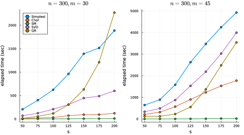
Figure 1: Elapsed times for local-search procedures

From Figure 1, we first observe that when $s$ increases in both plots (for $n=300,m=30$ and $n=300,m=45$) the times for the QR method (having complexity $\mathcal{O}(s^{2})$ per iteration) have a big increase confirming what is expected from theory. We also see that when $m$ increases from $30$ to $45$ all the methods show an increase in time, but for SM we have the smallest times and the smallest increase. It is interesting to note that when $m$ increases from $30$ to $45$, QR becomes more competitive for Chol. In fact, for $m=45$ and $s\leq 125$, QR is faster than Chol, while it is always slower when $m=30$. As QR has complexity $\mathcal{O}(s^{2})$ per iteration and Chol has complexity $\mathcal{O}(m^{2})$ per iteration, increasing $m$ is expected to increase more the times for Chol. The results point to SM as the most efficient method in our experiments. The second best method can be Chol or QR. As expected, both methods with complexity $\mathcal{O}(m^{3})$ per iteration (Simplest and SVD) have bad performance.

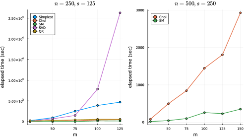
Figure 2: Elapsed times for local-search procedures

The superiority of SM is confirmed in Figure 2, where we vary $m$. We see that SVD (having complexity $\mathcal{O}(m^{3})$ per iteration) becomes very inefficient in comparison to the other methods when $m=100$ or $125$, for $n=250,s=125$. The plot in the right ($n=500,s=250$) compares the two methods with complexity $\mathcal{O}(m^{2})$ per iteration and we see again a better performance when using SM for this larger instance.

In Figure 3, we compare the three methods with complexity $\mathcal{O}(m^{2})$ per iteration when $s=m$ (in this case, we set $u=\mathbf{e}$). In that regime, we confirm that SM is the best option for our use and that there is no winner between QR and Chol.

From these experiments, we see that an efficient implementation of the procedure to update the computation of the determinant can have a significant impact in the efficiency of the local-search procedures.

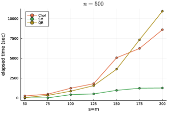
Figure 3: Elapsed times for local-search procedures

6.2 Comparing the versions of branch-and-bound

In Table 1, we analyse the impact of the procedures “VBT”, “LSI”, “LSC”, and “HS” on the performance of the branch-and-bound algorithm. On the first row of the table, we identify the seven versions of the branch-and-bound algorithm that were executed. On the next four rows, we identify which procedures are running in the branch-and-bound for each version. Then, we present the elapsed time to solve the instances and the number of nodes on the branch-and-bound enumeration tree for each version of the algorithm. The parameters $n,m,s$ of each instance are presented in the first column of the table.

When comparing versions (1)–(4) to versions (5)–(7), we see that the most successful procedure is LSC. When adding it to the branch-and-bound algorithm both the time and the number of nodes decrease significantly in general. When applying VBT to the branch-and-bound algorithm already with the LSC procedure included (version (6)), we have another decrease in time and number of nodes for most instances and this is the most successful procedure on our tests. We see that both LCI and HS are not effective in reducing neither the time nor the number of nodes. In fact, we observed that running the local-search procedures only when an integer solution is obtained during the execution of branch-and-bound, rarely improves the current lower bound on the objective value of D-Opt. Moreover, the Hadamard and the spectral bounds are rarely stronger than the continuous bound.

BB version	(1)	(2)	(3)	(4)	(5)	(6)	(7)
VBT		$\checkmark$	$\checkmark$	$\checkmark$		$\checkmark$	$\checkmark$
LSI			$\checkmark$	$\checkmark$
LSC					$\checkmark$	$\checkmark$	$\checkmark$
HS				$\checkmark$			$\checkmark$
$n,m,s$	Elapsed time (sec)
20,5,10	3.49	3.50	3.52	3.67	2.68	2.57	3.18
20,5,10	0.34	0.56	0.45	0.56	0.37	0.40	0.54
20,5,10	4.73	5.82	5.93	6.16	5.25	3.16	3.64
30,7,15	161.81	42.47	42.74	45.10	171.56	40.72	43.61
30,7,15	18.90	11.72	12.14	12.59	22.67	9.11	11.04
30,7,15	1.45	2.47	2.62	2.60	1.73	1.81	2.66
50,12,25	469.31	353.17	390.00	377.00	467.12	394.20	389.87
50,12,25	139.08	142.24	153.82	148.98	141.37	145.74	146.67
50,12,25	34.40	34.46	38.22	36.29	30.17	30.57	31.19
60,15,30	72.78	60.10	64.32	61.85	34.91	51.91	51.66
60,15,30	27.05	32.82	33.79	33.12	25.81	37.64	36.84
60,15,30	27.69	37.11	40.77	37.23	35.83	45.08	45.90
80,20,40	421.14	595.66	622.47	591.38	258.11	211.35	219.96
80,20,40	602.43	1085.66	1128.50	1062.40	320.31	316.72	318.46
80,20,40	9579.26	12751.16	13301.99	14560.62	5088.98	4636.28	4719.10
$n,m,s$	Number of nodes
20,5,10	191	125	125	125	121	103	103
20,5,10	3	3	3	3	3	3	3
20,5,10	337	303	303	303	315	219	219
30,7,15	10901	3113	3113	3091	10901	3113	3091
30,7,15	1467	683	683	683	1467	683	683
30,7,15	37	37	37	37	37	37	37
50,12,25	23245	17755	17755	17755	23245	17755	17755
50,12,25	6027	5331	5331	5331	5445	4969	4969
50,12,25	1513	1221	1221	1221	1077	919	919
60,15,30	2975	1557	1557	1557	889	833	833
60,15,30	569	463	463	463	309	403	403
60,15,30	531	591	591	591	531	591	591
80,20,40	6955	6245	6245	6245	2845	1897	1897
80,20,40	9013	11101	11101	11101	2995	2857	2857
80,20,40	174481	178609	178609	178609	72635	62905	62905

Table 1: Branch-and-bound (BB) algorithms

In Table 2, we present for each instance, the elapsed time to execute the local-search procedures (“LS”), the branch-and-bound algorithm, which corresponds to version (6) on Table 1 (“BB(6)”), and to solve the continuous relaxation (1) with Knitro at the root node at the branch-and-bound tree (“${z}^{\mathcal{C}}$”). We also present the objective value obtained with each procedure. Finally, column “VBT” shows the number of VBT inequalities that were effective in tightening the bounds of a variable during the execution of the branch-and-bound algorithm, and column “FV” shows the number of variables fixed by the VBT inequalities. The times for the local-search procedures corresponds to the execution of the three procedures described in Section 3.3, each starting from each of the four initial solutions presented in Section 3.1. The objective value corresponds to the best solution found. We see that the local-search procedures are very fast compared to the branch-and-bound algorithm and obtain solutions of very good quality even for the largest instances. The continuous relaxation is also solved in less than 1 second for all the instances and give tight bounds for the instances tested. Finally, we see that the VBT inequalities are effective and fix a significant number of variables.

	Elapsed time (sec)			Objective value			VBT	FV
$n,m,s$	LS	BB(6)	${z}^{\mathcal{C}}$	LS	BB(6)	${z}^{\mathcal{C}}$	BB(6)
20,5,10	0.012	2.572	0.020	5.754	5.768	5.802	71	49
20,5,10	0.007	0.403	0.012	6.206	6.206	6.226	32	32
20,5,10	0.007	3.155	0.016	5.645	5.696	5.735	30	27
30,7,15	0.041	40.715	0.027	8.484	8.484	8.549	445	371
30,7,15	0.025	9.109	0.023	8.549	8.549	8.604	192	138
30,7,15	0.025	1.806	0.016	9.186	9.186	9.232	125	89
50,12,25	0.110	394.195	0.039	13.660	13.660	13.712	6310	5838
50,12,25	0.208	145.736	0.038	13.454	13.457	13.543	2852	2493
50,12,25	0.110	30.568	0.042	14.100	14.104	14.180	868	727
60,15,30	0.341	51.914	0.059	16.744	16.750	16.779	1033	834
60,15,30	0.424	37.639	0.070	16.960	16.975	17.017	492	378
60,15,30	0.252	45.080	0.050	17.083	17.083	17.162	591	348
80,20,40	0.898	211.346	0.147	21.521	21.607	21.707	3581	2696
80,20,40	0.881	316.715	0.147	21.411	21.553	21.670	3981	3052
80,20,40	0.937	4636.277	0.107	21.610	21.671	21.789	55275	47219

Table 2: Performance of local search, branch-and-bound version (6), and VBT inequalities

7 Conclusion

Our numerical experiments indicate promising directions to investigate in order to improve the efficiency of the branch-and-bound algorithm to solve the D-optimality problem. One possible approach, for example, is to introduce the use of bounds from [15] when $\sum_{\ell\in\hat{N}}\hat{x}_{\ell}v_{\ell}v_{\ell}^{{\mathchoice{\raisebox{0.0pt}{$\displaystyle\mathsf{T}$}}{\raisebox{0.0pt}{$\textstyle\mathsf{T}$}}{\raisebox{0.0pt}{$\scriptstyle\mathsf{T}$}}{\raisebox{0.0pt}{$\scriptscriptstyle\mathsf{T}$}}}}$ is positive definite, where $x_{\ell}$ is fixed at $\hat{x}_{\ell}$ at a given subproblem, for all $\ell\in\hat{N}\subset N$.

References

- [1] Kurt M. Anstreicher. Maximum-entropy sampling and the Boolean quadric polytope. Journal of Global Optimization, 72(4):603–618, 2018.
- [2] Kurt M. Anstreicher. Efficient solution of maximum-entropy sampling problems. Operations Research, 68(6):1826–1835, 2020.
- [3] Kurt M. Anstreicher, Marcia Fampa, Jon Lee, and Joy Williams. Using continuous nonlinear relaxations to solve constrained maximum-entropy sampling problems. Mathematical Programming, 85:221–240, 1999.
- [4] Matthew Brand. Fast low-rank modifications of the thin singular value decomposition. Linear Algebra and its Applications, 415(1):20–30, 2006.
- [5] William F. Caselton and James V. Zidek. Optimal monitoring network design. Statistics and Probability Letters, 2:223–227, 1984.
- [6] Marcia Fampa and Jon Lee. Maximum-Entropy Sampling: Algorithms and Application. Springer, 2022.
- [7] Marcia Fampa, Jon Lee, Gabriel Ponte, and Luze Xu. Experimental analysis of local searches for sparse reflexive generalized inverses. Journal of Global Optimization, 81:1057–1093, 2021.
- [8] Valerii V. Fedorov. Theory of optimal experiments. Academic Press, New York-London, 1972. Translated from the Russian and edited by W. J. Studden and E. M. Klimko.
- [9] Gene H. Golub and Charles F. Van Loan. Matrix Computations (3rd Ed.). Johns Hopkins University Press, Baltimore, MD, USA, 1996.
- [10] Chun-Wa Ko, Jon Lee, and Kevin Wayne. A spectral bound for D-optimality, 1994. Unpublished.
- [11] Chun-Wa Ko, Jon Lee, and Kevin Wayne. Comparison of spectral and Hadamard bounds for D-optimality. In MODA 5, Contrib. Statist., pages 21–29. Physica, Heidelberg, 1998.
- [12] Ole Kröger, Carleton Coffrin, Hassan Hijazi, and Harsha Nagarajan. Juniper: An open-source nonlinear branch-and-bound solver in julia. In Integration of Constraint Programming, Artificial Intelligence, and Operations Research, pages 377–386. Springer International Publishing, 2018.
- [13] Jon Lee. Maximum entropy sampling. In A.H. El-Shaarawi and W.W. Piegorsch, editors, Encyclopedia of Environmetrics, 2nd ed., pages 1570–1574. Wiley, Boston, 2012.
- [14] Jon Lee and Joy Lind. Generalized maximum-entropy sampling. INFOR: Information Systems and Operational Research, 58(2):168–181, 2020.
- [15] Yongchun Li, Marcia Fampa, Jon Lee, Feng Qiu, Weijun Xie, and Rui Yao. D-optimal data fusion: Exact and approximation algorithms, 2022. Preprint arXiv:2208.03589.
- [16] Gabriel Ponte, Marcia Fampa, and Jon Lee. Exact and heuristic solution approaches for the D-optimality problem. In Proceedings of the LIV Brazilian Symposium on Operations Research, volume 54. SOBRAPO, Rio de Janeiro, RJ, Brazil, Nov 2022.
- [17] Friedrich Pukelsheim. Optimal Design of Experiments, volume 50 of Classics in Applied Mathematics. Society for Industrial and Applied Mathematics (SIAM), Philadelphia, PA, 2006. Reprint of the 1993 original.
- [18] Michael C. Shewry and Henry P. Wynn. Maximum entropy sampling. Journal of Applied Statistics, 46:165–170, 1987.
- [19] William J. Welch. Branch-and-bound search for experimental designs based on D-optimality and other criteria. Technometrics, 24(1):41–48, 1982.