The Stokes-Einstein-Sutherland equation at the nanoscale revisited

Abstract

The Stokes-Einstein-Sutherland (SES) equation is at the foundation of statistical physics, relating a particle’s diffusion coefficient and size with the fluid viscosity, temperature and the boundary condition for the particle-solvent interface. It is assumed that it relies on the separation of scales between the particle and the solvent, hence it is expected to break down for diffusive transport on the molecular scale. This assumption is however challenged by a number of experimental studies showing a remarkably small, if any, violation, while simulations systematically report the opposite. To understand these discrepancies, analytical ultracentrifugation experiments are combined with molecular simulations, both performed at unprecedented accuracies, to study the transport of buckminsterfullerene C₆₀ in toluene at infinite dilution. This system is demonstrated to clearly violate the conditions of slow momentum relaxation. Yet, through a linear response to a constant force, the SES equation can be recovered in the long time limit with no more than $4\text{\,}\mathrm{\char 37\relax}$ uncertainty both in experiments and in simulations. This nonetheless requires partial slip on the particle interface, extracted consistently from all the data. These results, thus, resolve a long-standing discussion on the validity and limits of the SES equation at the molecular scale.

I Introduction

Diffusion was first described by Robert Brown in 1827 [1], who observed jittering of small particles in water. The fundamental framework for this phenomenon, however, emerged only a century later due to contributions of Einstein [2], Sutherland [3] and von Smoluchowski [4]. Firstly, the Stokes-Einstein-Sutherland (SES) equation was developed relating the diffusion coefficient to temperature and the Stokes force acting on the moving particle. Secondly, Einstein and Smoluchowski provided the keystone for the fully probabilistic formulation of diffusion. The latter was experimentally confirmed by Jean-Baptiste Perrin and his students in 1908 [5, 6, 7, 8].

While very simple, easy to use and often applied for particle size determination [9, 10, 11, 12, 13], the SES equation applies in the thermodynamic limit and requires a separation of scales between the particle and the solvent in terms of mass and size [14, 15, 16]. Therefore, it should break down for diffusive transport at the molecular scale. Surprisingly, however, experimental studies often confirm the appropriateness of the SES prediction for molecular diffusion, despite the clear limits imposed by the theoretical framework [17].

The paradigmatic systems for studies of the SES equation have been the buckminsterfullerenes due to their stability and well-defined shape. Specifically, Soret forced Rayleigh scattering was used to measure the diffusion coefficient of C₆₀ in o-dichlorobenzene  [18]. They compared the radius of C₆₀, extracted using the SES equation, to partial molecular volume measurements [19]. With measurement errors of up to $10\text{\,}\mathrm{\char 37\relax}$, their measured deviation of the SES equation was less than $15\text{\,}\mathrm{\char 37\relax}$, using slip boundary conditions on the particle-solvent interface.

C₆₀ as well as C₇₀ was used again more recently to verify the performance of the SES equation in analytical ultracentrifugation (AUC) experiments [20]. Deviations of only about $5\text{\,}\mathrm{\char 37\relax}$ were found, this time with stick boundary conditions. The reference size of fullerenes was taken from the size of the rigid carbon shell [21, 22, 23, 24, 25, 26], which notably ignore solvation effects. Furthermore, in these experiments, neither finite concentration effects of C₆₀ and C₇₀ have been taken into account nor has the statistical significance of the results been checked. Finally, the choice of the boundary conditions was restricted to stick or slip with the conclusion that stick boundary conditions provide better results.

An alternative approach to study the limits of the SES equation are molecular dynamics (MD) simulations. They are the ideal tool for this task because they explicitly account for the atomic nature of the interactions, as well as for all the relevant time and length scales. However, unlike experiments, MD simulations systematically demonstrate discrepancies from the SES equation for small particles [27, 28, 29, 30, 31, 32, 33, 34, 35, 16]. However, the accuracy of the results was often questioned due to finite system sizes [27, 29, 31, 30], and limited sampling [30, 32, 35] of slowly convergent power law decays [36]. Interestingly, systematic simulation studies of fullerenes have not yet been performed. In order to understand the apparently small deviations of the SES equation in experiments, and large deviations in simulations, we here perform AUC measurements as well as MD simulations of C₆₀ suspended in toluene. Our aim is to combat issues of accuracy and sampling to explore the implication of different physical assumptions in modeling and measuring diffusion on the molecular scale as well as the influence of the partial molecular volume. This joint experimental and theoretical effort allows us to address the applicability of the SES equation in the infinite dilution limit, and use the precise analysis to determine the appropriate boundary conditions at the fullerene-solvent interface. We are, therefore, able to explore advantages and limitations of each approximation used to define the SES equation and hence provide a clear explanation of systematic discrepancy between experimental and modeling efforts appearing over the several decades.

II Stokes-Einstein-Sutherland equation and equilibrium statistical mechanics

sec:theory

II.1 Theoretical consideration

In 1905, both Einstein [2] and Sutherland [3] published the well-known relation between the diffusion and friction coefficients $D$ and $\xi$, respectively, of a particle in a solvent

$$\zlabel{eq:intro:einstein}D=\frac{k_{\textup{B}}T}{\xi}\>.$$ (1)

Here, $T$ is the temperature and $k_{\textup{B}}$ the Boltzmann constant. Both Einstein and Sutherland used the Stokes’ formula to express the friction coefficient as a function of the fluid shear viscosity $\eta$ and the hydrodynamic radius $R_{\textup{H}}$ of the particle, which was assumed to be spherical:

$$\zlabel{eq:intro:stokes}\xi=b\pi\eta R_{\textup{H}}\>.$$ (2)

The prefactor $b$ is a function of the boundary condition on the particle-solvent interface and ranges from $4$ for a perfect slip to $6$ for a perfect stick boundary condition, as used by Stokes’ [37] and Einstein [2]. Finally, by combining equations (eq:intro:einstein) and (eq:intro:stokes) one obtains the SES equation

$$\zlabel{eq:intro:ses}D=\frac{k_{\textup{B}}T}{b\pi\eta R_{\textup{H}}}\>,$$ (3)

for the diffusion coefficient of a particle dispersed in a liquid.

This approach surprisingly well relates molecular fluctuations, characterized by diffusion, with a highly coarse grained hydrodynamic friction, where molecular details are no longer resolved. Instead, they are incorporated into the boundary condition $b$. The friction itself is defined as the ratio of a force $F$ acting on the particle and the velocity $v$ resulting from this force

$$\zlabel{eq:intro:friction}\xi=\frac{F}{v}\>.$$ (4)

Already in the original derivation [2, 3], the force acting on the particle was presumed to arise from its collisions with the solvent molecules that in equilibrium should average to zero in the long time limit.

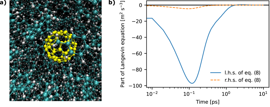
Figure 1: C₆₀ in toluene as a model for studying molecular diffusion. a) The system in question: a single C₆₀ (colored in yellow) is dispersed in toluene. b) Comparison between left and right hand side of equation (eq:LE-autocorr). The left hand side is nearly $20$ times larger than the right hand side. In addition, the sign is different in the regime from $1.0\text{\,}\mathrm{ps}1.7\text{\,}\mathrm{ps}$, demonstrating that the momentum of C₆₀ cannot be treated as a slow variable. Ensemble averages cover 3-dimensional trajectories of the same system size with $3824$ solvent molecules and a total simulation time of $\approx$35\text{\,}\mu\mathrm{s}$$.

fig:system

Significant progress in understanding the relation of transport coefficients to microscopic degrees of freedom as well as the limits of applicability of the SES equation in terms of involved time and length scales was achieved using techniques from statistical mechanics [38, 39, 40, 41, 42, 43, 14, 44]. Building on the molecular theory, it became possible to express transport coefficients as integrals of autocorrelation functions of a corresponding dynamic variable using the so called Green-Kubo (GK) relations [38, 39, 40, 42]. For example, the shear viscosity could be calculated from the off-diagonal elements of the stress tensor $P_{\alpha\beta}$

$$\zlabel{eq:gk-visco}\eta=\frac{V}{k_{\textup{B}}T}\int_{0}^{\infty}\langle P_{\alpha\beta}(t)P_{\alpha\beta}(0)\rangle\mathrm{d}t\>,$$ (5)

where the brackets $\langle.\rangle$ denote an ensemble average. Most notably, the diffusion coefficient was found to be related to the velocity autocorrelation function (VACF) with

$$\zlabel{eq:gk-diff}D_{\textup{VACF}}=\int_{0}^{\infty}\langle v(t)v(0)\rangle\mathrm{d}t\>,$$ (6)

while the friction coefficient was related to the stochastic force $F_{\textup{S}}(t)$ acting on the particle of interest through its autocorrelation function (ACF) [38, 43, 44, 45]

$$\zlabel{eq:gk-fric}\xi=\frac{1}{k_{\textup{B}}T}\int_{0}^{\infty}\langle F_{\textup{S}}(0)F_{\textup{S}}(t)\rangle\mathrm{d}t\>,$$ (7)

The latter equation can be obtained from a general Langevin equation

$$\frac{\partial}{\partial t}p(t)=-\int_{0}^{t}\mathrm{d}sK(s)p(t-s)+F_{\textup{S}}(t)\>,$$ (8)

where $p(t)$ is the particle momentum, $K(s)$ the memory kernel and $F_{\textup{S}}(t)$ a stochastic force acting on the particle. The fluctuation-dissipation theorem relates the memory kernel to the stochastic force via

$$\langle F_{\textup{S}}(t)F_{\textup{S}}(t^{\prime})\rangle=3k_{\textup{B}}TK(t-t^{\prime})$$ (9)

and the integral of the memory kernel yields equation (eq:gk-fric). Obtaining the stochastic force autocorrelation function (F_SACF), required for the memory kernel, from simulations or experiments is a non-trivial task [46]. However, upon deriving this formula via the projection operator formalism [44, 45] (cf. SI section sec:si:mori-zwanzig for the derivation), and assuming a small rate of change of the particle momentum, i.e.

$$\frac{\partial}{\partial t}p(t)=\mathcal{O}(\lambda)$$ (10)

with some small parameter $\lambda$, the F_SACF can be approximated with the total force autocorrelation function (F_TACF)

$$\langle F_{\textup{S}}(t)F_{\textup{S}}(t^{\prime})\rangle=\langle F_{\textup{T}}(t)F_{\textup{T}}(t^{\prime})\rangle+\mathcal{O}\left(\lambda^{3}\right)$$ (11)

upon neglecting orders of $\lambda^{3}$ and higher. The total force $F_{\textup{T}}$ is easily accessible through Newton’s equation $F_{\textup{T}}=\partial p/\partial t$, especially from MD simulations, where it is a prognostic variable. The friction coefficient is then given as

$$\zlabel{eq:gk-fric-ftacf}\xi=\frac{1}{k_{\textup{B}}T}\int_{0}^{\infty}\langle F_{\textup{T}}(0)F_{\textup{T}}(t)\rangle\mathrm{d}t\>.$$ (12)

Notably, it was shown, that the zero frequency component of the F_TACF and hence its time integral, will be non-zero if and only if the limit $\lambda\rightarrow 0$ is strictly fulfilled [38, 43, 15, 47, 48], which corresponds to a particle with constant momentum, often referred to as the frozen particle. Nonetheless, invoking Stokes’ formula (eq:intro:stokes) for a particle with constant, non-zero momentum also fulfills this limit. Furthermore, both the ACFs of velocity (eq:gk-diff) and position (not shown here) do have a zero frequency component and can thus be used to obtain the friction coefficient [48], which is equivalent to invoking the Einstein-Sutherland equation. The statistical approach therefore provides equation (eq:intro:einstein) from first principles, and sets the limits of applicability of the SES equation.

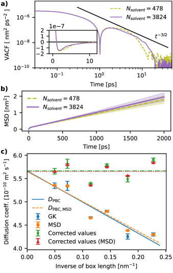
Figure 2: Diffusion coefficient of C₆₀ in toluene obtained from MD simulations. a) Log-log representation of the absolute value of the VACF for two different system sizes (inverse of box length: $\approx$0.23\text{\,}{\mathrm{nm}}^{-1}$$ and $0.11\text{\,}{\mathrm{nm}}^{-1}$). The analysis runs over $6\text{\,}\mathrm{\SIUnitSymbolMicro s}$ and $35\text{\,}\mathrm{\SIUnitSymbolMicro s}$ 3-dimensional trajectory, for the small and large systems, respectively. Especially for the larger system, the expected decay proportional to $t^{-3/2}$ is apparent for times $>$2\text{\,}\mathrm{ps}$$ [36]. The inset shows a lin-lin representation of the VACF in the region around the first minimum. b) MSD for the same system sizes as in a). Due to finite size effects, the larger system produces a larger MSD and diffusion coefficient (cf. panel c). c) Size dependence of the diffusion coefficient. Equation (eq:diff-size_dependence) is used for both the fit (lines) and the corrected values. Symbols represent mean and standard deviation of the plateau region for a single system size each (cf. SI-Figure fig:si:diff). The analysis runs over $6\text{\,}\mathrm{\SIUnitSymbolMicro s}$ to $35\text{\,}\mathrm{\SIUnitSymbolMicro s}$ 3-dimensional trajectory, for the different systems.

fig:results:diffusion

II.2 Molecular dynamics simulations

sec:md To assess how crucial the restriction of the constant particle momentum is, we reformulate the problem (cf. SI section sec:si:mori-zwanzig for the derivation), to obtain a Volterra equation of first kind, that can be directly checked from simulations:

$$\zlabel{eq:LE-autocorr}\frac{\partial}{\partial t}\langle p(t)p(0)\rangle=-\frac{1}{k_{\textup{B}}T}\int_{0}^{t}\mathrm{d}s\langle F_{\textup{T}}(s)F_{\textup{T}}(0)\rangle\cdot\langle p(t)p(0)\rangle\>.$$ (13)

This equation includes approximating the F_SACF with the F_TACF.

MD simulations are performed using the GROMACS simulation package [49, 50, 51, 52, 53, 54, 55], by placing a single C₆₀ in a box of toluene (cf. Figure fig:systema) and applying periodic boundary conditions (see SI section sec:si:methods for details). For toluene, we use the Optimized Potentials for Liquid Simulations (all atoms) (OPLS-AA) force field [56], while the parameters for C₆₀ are taken from previous work [57]. Following an extensive protocol to equilibrate the system at room temperature and $1\text{\,}\mathrm{bar}$, production simulations are performed in NVT ensemble with the temperature maintained by the Nosé-Hoover thermostat. We modify the output routine of GROMACS to simultaneously extract the total force on the particle and its momentum with the output rate of $10\text{\,}\mathrm{fs}$ without all solvent information. This accounts for C₆₀ internal forces and external van der Waals forces, while Coulomb forces are absent for the uncharged C₆₀ atoms. To take into account finite size effects we simulate an array of systems with 478 to 46838 toluene molecules (Figure fig:systema), for in total $0.6\text{\,}\mathrm{\SIUnitSymbolMicro s}35\text{\,}\mathrm{\SIUnitSymbolMicro s}$, and apply the appropriate finite size corrections [58, 59]. Using the system isotropy, averaging over all spatial dimensions is performed to improve the statistics.

This methodology allows us to evaluate both sides of equation (eq:LE-autocorr) by numerical differentiation or integration. We find that this expression does not hold for a C₆₀ in toluene, which clearly demonstrates that the momentum is not a slowly changing variable (Figure fig:systemb). Thus, one could infer that the friction coefficient cannot be properly obtained by the GK approach, which becomes evident from directly evaluating equation (eq:gk-fric-ftacf). The full integral vanishes as expected [38, 48]. Other methods were previously suggested to calculate the friction coefficient from the running integral of the F_TACF [15, 32, 16], which worked for particles heavy compared to the solvent molecules but not necessarily infinitely heavy. In our case, neither a linear nor an exponential decay can be observed (cf. SI section sec:si:diffusion:facf and SI-Figure fig:results:facf) and thus the only of these methods left is using the maximum of the running integral, that corresponds to the first zero-crossing of the F_TACF, as suggested by Lagar'kov and Sergeev [60]. This method, known to be an overestimation [15, 32], yields with corrections for finite size effects (see SI section sec:si:finite-size and (eq:friction-size)) $\xi=$(3.37\pm 0.03)\text{\times}{10}^{-12}\text{\,}\mathrm{kg}\text{\,}{\mathrm{s}}^{-1}$$.

This can be verified by extracting the diffusion coefficient of C₆₀ from the VACF via the GK relation (eq:gk-diff) and the mean square displacement (MSD) (cf. SI section sec:si:diffusion:vacf) as both methods are well established [36, 16] (cf. Figure fig:results:diffusiona,b). We account for the finite size effects by the theoretical size dependence of the diffusion coefficient [58, 59], adjusted to include a variable boundary condition $b$

$$\zlabel{eq:diff-size_{d}ependence}D_{\infty}=D_{\textup{PBC}}+\frac{k_{\textup{B}}T\zeta}{b\pi\eta a}\>.$$ (14)

Using this equation, all data (cf. Figure fig:results:diffusionc) can be fitted (blue circles and orange squares) or corrected (green diamonds and red triangles). Hereby, the fit was calculated by treating both the boundary condition parameter $b$ and the infinite diffusivity $D_{\infty}$ as free parameters, yielding $D_{\infty}=$(5.67\pm 0.19)\text{\times}{10}^{-10}\text{\,}{\mathrm{m}}^{2}\text{\,}{\mathrm{s}}^{-1}$$ for the VACF and $D_{\infty}=$(5.65\pm 0.17)\text{\times}{10}^{-10}\text{\,}{\mathrm{m}}^{2}\text{\,}{\mathrm{s}}^{-1}$$ for the MSD. Unfortunately, the parameter $b$ carries a significant uncertainty, such that precise conclusions about the effective boundary condition cannot be made using this approach.

Using equation (eq:intro:einstein), we compare the obtained $D_{\infty}$, with the calculated $k_{\textup{B}}T/\xi$. We find deviations larger than $50\text{\,}\mathrm{\char 37\relax}$, due to the gross underestimation of the C₆₀ friction coefficient. This clearly shows that the standard approximations of equilibrium statistical physics underlying the SES equation do not hold in this system, presumably because of the similar mass of the C₆₀ and the toluene molecule.

As this deviation stems from the failure of approximating the memory kernel $K(s)$ with the F_TACF instead of the F_SACF, it is only natural to verify whether the memory kernel, if extracted with different methods [46], reproduces the correct friction coefficient. Several methods to derive the memory kernel for systems on the molecular scale have been developed in the past years [46]. We calculate $K(s)$ through the Fourier transform from the VACF, as suggested by [61, 46], which is equivalent to calculating the diffusion coefficient from the VACF and invoking the Einstein-Sutherland equation (eq:intro:einstein). For the system with 3824 solvent molecules, we obtain a clear deviation from the kernel obtained from the F_TACF (see SI-Figure fig:results:memory-kernela). By integrating the kernel from the VACF, we obtain $\xi_{\textup{PBC}}=$(8.68\pm 0.03)\text{\times}{10}^{-12}\text{\,}\mathrm{kg}\text{\,}{\mathrm{s}}^{-1}$$, which, by the Einstein-Sutherland equation (eq:intro:einstein), corresponds to a diffusion coefficient of $D_{\textup{PBC}}=$(4.66\pm 0.02)\text{\times}{10}^{-10}\text{\,}{\mathrm{m}}^{2}\text{\,}{\mathrm{s}}^{-1}$$, precisely the value obtained by integrating the VACF (both values are for the same system size and thus not corrected for system size effects). This expected agreement underlines the failure of approximating the F_SACF with the F_TACF for such small particles, while supporting the validity of the Einstein-Sutherland equation.

III Einstein-Sutherland equation under conditions of constant drag

III.1 Analytical ultracentrifugation experiments

sec:AUC

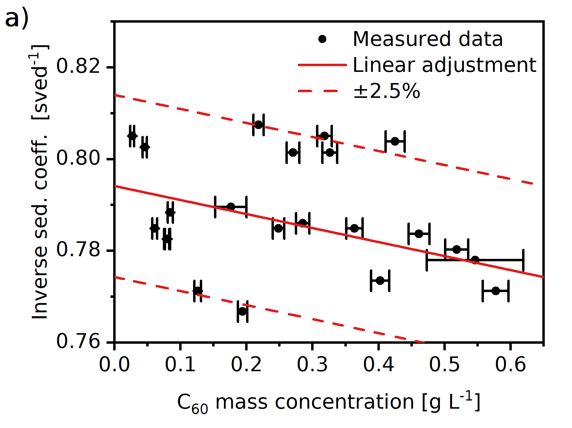
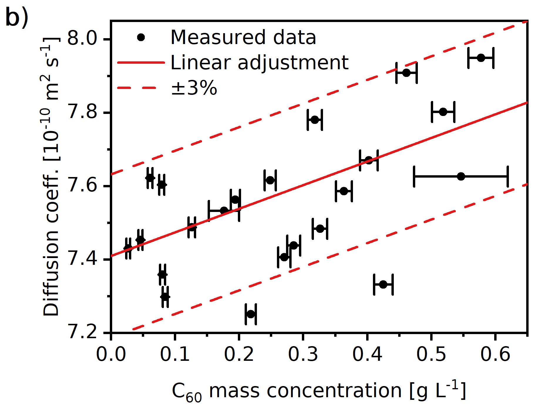
Figure 3: Retrieved inverse sedimentation coefficients (a) and diffusion coefficients (b) from SV-AUC experiments as a function of C₆₀ mass concentration. Depicted are hydro- and thermodynamic non-ideality of C₆₀ resulting from data-analysis with the $c(s)$-model (Levenberg-Marquardt). Linear fits were performed taking the uncertainty of the extinction, optical path length and the extinction coefficient at $570\text{\,}\mathrm{nm}$ for the concentrations into account. The corresponding uncertainty (standard deviation) is depicted with the symbols.

fig:results:AUC

There are several reports that validate the SES equation for C₆₀ in molecular solvents [17, 18, 20]. However, even these works differ in the choice of the boundary conditions and treatment of effects of finite concentration. This, together with the results of the previous section, calls for a discussion of the validity of the theory and/or the correct choice of parameters for comparison.

To clarify these issues, we perform a set of AUC experiments to observe the reaction of the system to a centrifugal field [62, 63, 64]. In this type of experiments, referred to as sedimentation velocity AUC (SV-AUC) experiments, we resolve the temporal evolution and radial distribution of the particles’ concentration (cf. SI section sec:si:auc-experiments). Using numerical solutions of the Lamm equation (eq:Lamm), we fit the data with the diffusion and sedimentation coefficients $D$ and $s$, respectively, while also considering compressibility of the solvent (cf. SI sections sec:si:auc-formulas, sec:si:auc-interpretation and sec:si:diffusion:auc for details). Conducting the experiment at different concentrations (Figure fig:results:AUC), allows us to retrieve the values extrapolated to infinite dilution by means of a linear fit to be $D_{0}=$7.41\pm 0.04\text{\,}{\mathrm{m}}^{2}\text{\,}{\mathrm{s}}^{-1}$$ and $s_{0}=$1.26\pm 0.01\text{\,}\mathrm{s}\mathrm{v}\mathrm{e}\mathrm{d}$$. The single sample measurement of Pearson et al. [20] at a finite concentration, which we estimate to be about $1\text{\,}\mathrm{g}\text{\,}{\mathrm{l}}^{-1}$, yields $D_{\textup{Pearson}}=$7.59\text{\,}{\mathrm{m}}^{2}\text{\,}{\mathrm{s}}^{-1}$$, which is fully consistent with our data.

However, direct comparison of the measured diffusion coefficients to simulation results (section sec:md) shows significant differences. This discrepancy can be attributed to the $1.4$ times higher viscosity of toluene provided by the OPLS-AA force field [56] (see SI section sec:si:diffusion:viscosity) compared to experimental reference measurements at same thermodynamic conditions of a temperature of $293.15\text{\,}\mathrm{K}$ and pressure of $1\text{\,}\mathrm{bar}$ [65]. We can, nonetheless, normalize the diffusion coefficient by the ratio of the MD and measured viscosity (SI section sec:si:diffusion:viscosity), which provides an agreement between the simulated and the experimental diffusivity with a deviation of less than $10\text{\,}\mathrm{\char 37\relax}$ (see Table tab:results:summary, column 4).

We can then obtain the friction coefficient directly from $s_{0}=m/\xi$, with $m$ being the excess mass of the analyte, i.e. the mass of the analyte minus the mass of solvent with the same volume. Ruelle et al. [19] measured the C₆₀ partial molecular volume in toluene to be $0.603\text{\,}{\mathrm{nm}}^{3}$, which combined with its molecular mass of $720.66\text{\,}\mathrm{u}$ and a toluene density of $866.86\text{\,}\mathrm{kg}\text{\,}{\mathrm{m}}^{-3}$ yields a friction coefficient of $5.35\text{\times}{10}^{-12}\text{\,}\mathrm{kg}\text{\,}{\mathrm{s}}^{-1}$. We can now compare this to the prediction of the Einstein-Sutherland equation (eq:intro:einstein) obtained from the diffusion coefficient of the AUC experiments, which gives $k_{\textup{B}}T/D_{0}=$5.46\text{\times}{10}^{-12}\text{\,}\mathrm{kg}\text{\,}{\mathrm{s}}^{-1}$$. Both results agree within $2\text{\,}\mathrm{\char 37\relax}$, clearly demonstrating the validity of the Einstein-Sutherland equation for this system, which was not explicitly shown before. We hypothesize that this estimate of friction stems from the non-equilibrium nature of the AUC experiment. Namely rather than the friction being measured as a response to the stochastic force, here it emerges from the response to a constant drag or centrifugal force acting on the C₆₀.

III.2 Friction as response to a drag force in non-equilibrium MD simulations

sec:diffusion:pull

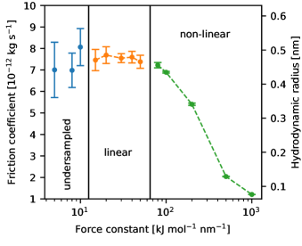
Figure 4: Friction coefficient of C₆₀ obtained from steered MD simulations. The friction coefficient $\xi_{\textup{PBC}}$ is calculated for each applied constant force as the ratio of applied force and resulting average velocity. Three regimes are indicated, the regime where statistics are not sufficient to determine a precise friction coefficient, the regime of proper linear response and the regime of non-linear response, where the apparent friction coefficient drops significantly. For the present study, only the linear regime is relevant and used to determine the friction coefficient as the mean over the entire range. Displayed error bars denote the uncertainty in the mean of the calculated friction coefficient, where the mean is calculated over a total of $40\text{\,}\mathrm{ns}200\text{\,}\mathrm{ns}$ trajectory. The hydrodynamic radius displayed corresponds to a boundary condition value of $c=6$.

fig:results:pull-friction

To verify our hypothesis that the friction coefficient can be determined if a particle is subject to a non-vanishing average force, we return to modeling and perform non-equilibrium molecular dynamics NEMD simulations. Specifically, an additional (constant) force on the fullerene is added while removing the center-of-mass motion of the entire system. The latter is required to obtain a proper frame of reference with periodic boundary conditions. The resulting particle velocity, relative to the fluid, is then calculated and combined with the known force to extract the friction coefficient $\xi$ from equation (eq:intro:friction).

To ensure, that we sample the linear regime, a set of pull forces is investigated (cf. Figure fig:results:pull-friction and SI section sec:si:diffusion:pull). For weak pull forces (blue points in Figure fig:results:pull-friction), the sampling is poor due to the small signal-to-noise ratio, while for large pull forces (green points), non-linear effects arise. For intermediate pull forces (orange points), we observe a properly converged and linear regime. Accounting for finite size effects (eq:friction-size) yields $\xi=$(6.9\pm 0.15)\text{\times}{10}^{-12}\text{\,}\mathrm{kg}\text{\,}{\mathrm{s}}^{-1}$$. Notably, this again compares well (about $10\text{\,}\mathrm{\char 37\relax}$ deviation) to the AUC result, when corrected for the differences in the viscosity (cf. section sec:AUC).

Importantly, we can calculate the diffusion coefficient from this friction coefficient with the Einstein-Sutherland equation (eq:intro:einstein) to obtain $D=$(5.9\pm 0.1)\text{\times}{10}^{-10}\text{\,}{\mathrm{m}}^{2}\text{\,}{\mathrm{s}}^{-1}$$, with the statistical error of $2\text{\,}\mathrm{\char 37\relax}$. This is basically the same result as the diffusion coefficient obtained from the MSD or the VACF (section sec:md). This confirms the validity of the Einstein-Sutherland equation found in the AUC experiments also for MD simulations, rendering both techniques consistent.

IV Stokes-Einstein-Sutherland equation

IV.1 The effective radius of C₆₀

sec:radius

Table 1: Summary of radii of the C₆₀ obtained by various methods. The radius $R_{\textup{graphite}}^{\textup{{exp}}}$ is obtained by adding half of the graphite interplanar distance to the radius of the structure of the C₆₀ nuclei, which gives the radius in the gas phase. The radius $R_{\textup{cryst}}^{\textup{{exp}}}$ is obtained by the fullerene distance in C₆₀ crystal. All radii $R_{V}$ are volume equivalent radii, i.e. radii corresponding to the partial molecular volume or the PSV.

Method	source	radius [$\mathrm{nm}$]
$R_{\textup{graphite}}^{\textup{{exp}}}$	[66, 67, 22, 23, 68, 24]	$0.522\pm 0.001$
$R_{\textup{cryst}}^{\textup{{exp}}}$	[69, 70, 25]	$0.52\pm 0.01$
$R_{\textup{V}}^{\textup{sim}}$	section sec:radius	$0.500\pm 0.003$
$R_{\textup{V}}^{\textup{exp, AUC}}$	section sec:radius	$0.520\pm 0.002$
$R_{\textup{V}}^{\textup{exp, DC SE}}$	section sec:si:radius	$0.526\pm 0.014$
$R_{\textup{V}}^{\textup{exp}}$	[19]	$0.524\pm 0.003$

tab:radii:summary

With the validity of the Einstein-Sutherland equation demonstrated for both experiments and NEMD simulations, the next step is to assess the validity of the SES equation and more importantly to retrieve a proper value for the boundary condition coefficient $b$. To assess this, we need to calculate and/or measure toluene viscosity (section sec:si:diffusion:viscosity), and the hydrodynamic radius of the C₆₀ independently from the friction and diffusion coefficients.

As the C₆₀ is a very rigid, nearly spherical molecule that does not feature extraordinarily strong interactions with the carbon-rich toluene, solvation effects in this specific environment were found to be very small compared to the C₆₀ in the solid phase [19]. This is reflected in sub-angstrom differences in radii $R_{V}$, that can be associated to a sphere with equivalent volume (cf. [66, 67, 22, 23, 68, 24, 69, 70, 25, 19], table tab:radii:summary and SI section sec:si:radius). Because of these small differences, $R_{V}$ has been used as the estimate for the C₆₀ hydrodynamic radius $R_{H}$ [20].

To verify these results and validate our own simulation and experimental protocols, we pursue the independent calculation of the partial molecular volume. In simulations, the partial molecular volume can be obtained from the particle-solvent radial distribution function (RDF) $g(r)$ via a Kirkwood-Buff integral [71]

$$\zlabel{eq:radius-kb}V=\frac{4}{3}\pi R_{\textup{V}}^{3}=\frac{1}{n_{\textup{s}}}+4\pi\int_{0}^{\infty}[g_{\textup{s}}(r)-g(r)]r^{2}\mathrm{d}r\>,$$ (15)

with $g_{\textup{s}}(r)$ being the RDF of the pure solvent and $n_{\textup{s}}$ the number density of the solvent (cf. SI-Figure fig:results:psva). This provides $R_{\textup{V}}^{\textup{{sim}}}=$0.500\pm 0.003\text{\,}\mathrm{nm}$$, deviating from the experimental reference [19] by only $4\text{\,}\mathrm{\char 37\relax}$.

We, furthermore, independently determine the C₆₀ radius in experiments, using sedimentation equilibrium AUC (SE-AUC) experiments with density contrast. In these measurements, the rotor speed and thus centrifugal force is sufficiently small such that the sedimentation flux compensates the diffusion flux at each radial position. From the resulting exponential concentration profile, the apparent buoyant mass can be calculated independent of the viscosity. Using solvents with different levels of deuteration, which changes solvent density but not the solvation properties of dissolved species, the PSV can be obtained. Due to a small number of parameters and thus small statistical uncertainties, the relevant data can be obtained with high accuracy yielding $R_{\textup{V}}^{\textup{exp, DC}}=$0.526\pm 0.014\text{\,}\mathrm{nm}$$, which is within measurement errors of less than $3\text{\,}\mathrm{\char 37\relax}$ compared to literature results obtained using different methods [19], and only $5\text{\,}\mathrm{\char 37\relax}$ different to the simulation data. Finally to check the consistency of our SV-AUC experiments, we retrieve the PSV directly from the diffusion and sedimentation coefficients at the infinite dilution limit by rearranging the well-known Svedberg equation (eq:Svedberg) to solve for the PSV (eq:psv-auc). This gives $R_{\textup{V}}^{\textup{exp, AUC}}=$0.520\pm 0.002\text{\,}\mathrm{nm}$$. Notably, this is within measurement errors of less than $1\text{\,}\mathrm{\char 37\relax}$ equivalent to the values obtained with our other approaches and the literature [19] (cf. Table tab:radii:summary).

IV.2 Effective boundary condition at the C₆₀ toluene interface

sec:boundary-condition

Table 2: Summary of diffusion coefficients and boundary conditions of the C₆₀ obtained by various methods. Values derived using (eq:intro:einstein) are indicated by superscripts. All values except for the one obtained from the F_TACF match. We find the averaged value of $\bar{b}=$5.5\pm 0.2$$ (cf. section sec:boundary-condition) to be consistent with all other presented data.

Method	source	diffusivity	rescaled diffusivity	$b$ from SES
		[${10}^{-10}\text{\,}{\mathrm{m}}^{2}\text{\,}{\mathrm{s}}^{-1}$]	[${10}^{-10}\text{\,}{\mathrm{m}}^{2}\text{\,}{\mathrm{s}}^{-1}$]	[-]
FTACF	section sec:si:diffusion:facf	$12.0\pm 0.1$	$17.4\pm 0.2$	$2.53\pm 0.04$
VACF, MSD	section sec:md	$5.7\pm 0.2$	$8.2\pm 0.3$	$5.3\pm 0.2$
Pulling force	section sec:diffusion:pull	$5.9\pm 0.1$	$8.5\pm 0.2$	$5.2\pm 0.2$
AUC exp.	section sec:si:diffusion:auc	$7.41\pm 0.04$	$7.41\pm 0.04$	$5.71\pm 0.06$
AUC exp.	[20]	$7.59$	$7.59$	$5.54\pm 0.03$

tab:results:summary

With these referent values for the C₆₀ size, we can now proceed with the determination of the boundary condition at the particle-solvent interface. For the AUC experiments, the boundary condition value can be retrieved directly from the well-known frictional ratio $\xi/\xi_{0}$, which is also known as $f/f_{0}$ in the AUC literature. It is defined as the ratio of the friction coefficient of the analyte to the friction coefficient of a sphere of equal volume as the analyte and assuming stick boundary conditions. When expressed in terms of $s$ and $D$ and using the PSV $\bar{\nu}$ of the fullerene, one obtains for spherical particles the well-known form:

$$\zlabel{eq:frictional_{r}atio}\xi/\xi_{0}=\left(\frac{\sqrt{2}}{18\pi}\frac{k_{\textup{B}}T}{D\sqrt{s}\eta^{\frac{3}{2}}}\sqrt{\frac{1-\bar{\nu}\rho}{\bar{\nu}}}\right)^{\frac{2}{3}}=$0.95\pm 0.01$$$ (16)

The frictional ratio is typically used to evaluate shape anisotropy and volume expansion due to solvation, when $\xi/\xi_{0}\geq 1$ [63]. With the nearly perfect spherical shape of C₆₀ and hardly any volume expansion effects (see SI sections sec:si:radius:static and sec:si:radius), we expect a value very close to unity. However, values $\xi/\xi_{0}<1$, on the other hand, point to deviations from the stick boundary condition. Indeed, when assuming $R_{\textup{H}}=R_{\textup{V}}$, we obtain $b=6\cdot\xi/\xi_{0}=$5.71\pm 0.06$$.

We can furthermore determine the boundary condition $b$ at the C₆₀–toluene interface, such that the SES equation holds, also from simulations. Using $D_{\textup{VACF}}$ or $D_{\textup{MSD}}$ and equation (eq:intro:ses), with $R_{\textup{H}}=R_{\textup{V}}$ determined in simulations, we obtain $b=$5.3\pm 0.2$$. Following a similar strategy, we can combine experimental data in the literature ($R_{\textup{V}}^{\textup{exp}}$ [19] and $D_{\textup{AUC}}$ [20]), and obtain $b=$5.54\pm 0.03$$, which is within the error bar of the simulation and only $3\text{\,}\mathrm{\char 37\relax}$ smaller than our experimental results.

Due to significant accuracy of the measurements and simulations, these results clearly indicate that perfect stick boundary conditions, typically assumed in experiments [20, 17, 72, 73, 74, 75, 76] and simulations [27, 28, 33, 34, 35], may not be the correct choice for C₆₀. Actually, with $b=6$ systematic errors of $5\text{\,}\mathrm{\char 37\relax}12\text{\,}\mathrm{\char 37\relax}$ are found in simulations and experiments. Furthermore, $R_{\textup{H}}$ calculated from the SES is found to be smaller than $R_{\textup{V}}$.

Finding deviations from the stick boundary conditions should not be surprising in the light of a long going discussion on its application for small particles [77]. The argument is captured by the Knudsen number $\mathit{Kn}$, the latter being defined as the ratio of mean free path and size of a particle. It can be calculated as $\mathit{Kn}=(\sqrt{2}\pi nd^{2}l)^{-1}$, where $n$ and $d$ are number density and diameter of the solvent, while $l$ is the characteristic length of the system. With $d$ taken to be the diameter of the toluene aromatic ring and $l$ the diameter of the fullerene, we estimate $\mathit{Kn}\approx$0.09$$. This is significant because the Knudsen number can be used as a measure to determine $b$ [72]. Specifically for $\mathit{Kn}=0$, one expects perfect stick ($b=6$) while for $\mathit{Kn}\rightarrow\infty$, perfect slip ($b=4$). As soon as $\mathit{Kn}$ is not vanishing, as in the present case, $b<6$ should be obtained, which is indeed the case.

V Discussion and Conclusions

sec:conclusions We here present a set of experimental and simulation results on the dynamic and static properties of a C₆₀ dispersed in toluene. We perform AUC experiments reporting diffusion and sedimentation coefficients in the infinite dilution limit, improving on the accuracy of the method [20]. Instead of following the usual approach to AUC data, and calculating the particle mass and size, we use the known mass of C₆₀ to report the hydrodynamic radius and the boundary condition at the particle-solvent interface. We furthermore perform a quantitative comparison of simulations and experiments which is excellent for static properties derived from density distributions. This includes the determination of the partial molecular volume of C₆₀, which differs from the experimental estimate by only a couple of percent. Extracting dynamic properties such as viscosity is more challenging due to the limitation of current force fields. However, upon simple re-scaling by the viscosity contrast (column 4 in Table tab:results:summary) the difference between observed and measured diffusivities is only $10\text{\,}\mathrm{\char 37\relax}$. Furthermore, the analysis which does not rely on correcting for the viscosity contrast, allows us to make several important findings:

• The expression associating the force autocorrelation function (FACF) and the friction coefficient suggested by Kirkwood [38], the Green-Kubo theory [39, 40, 41, 42] and the Mori-Zwanzig formalism [43, 14, 44] is the main starting point for the critique on the applicability of the SES equation at the nanoscale. In its derivation, the assumption that the particle momentum is constant, or only very slowly changing, is mandatory. We show that this assumption is clearly violated for C₆₀ in toluene due to its small molecular weight  [15, 47], back-scattering and dissipation of momentum through internal degrees of freedom that couple with directional motions on sub-picosecond time scales (Figure fig:systemb). The F_TACF integrates these effects, resulting in a vanishing response of the zero frequency component and thus, in this formulation, cannot be directly related to friction. If, contrastingly, the memory kernel is obtained from the F_SACF or via a different method [46, 61], the actual friction coefficient can be obtained.

• Another reliable measurement of the friction coefficient, however, can be obtained in non-equilibrium conditions. The good estimate can be extracted from the average velocity of C₆₀ induced by a drag force in the linear response. This is permitted by the momentum conservation and the nanosecond sampling times when conditions of slow dynamics are recovered (Figure fig:systemb). In experiments, the non-equilibrium conditions are provided in the sedimentation experiments, while in simulations, the friction is obtained in steered molecular dynamics (following equation (eq:intro:friction)). Using the Einstein-Sutherland relation, we can compare this friction to independently measured diffusion constants. For experiments, where infinite dilution sedimentation and diffusion coefficients are extracted by a sequence of measurements, the Einstein-Sutherland equation is recovered with $1\text{\,}\mathrm{\char 37\relax}$ accuracy. In simulations, by accounting for finite size effects, the Einstein-Sutherland relation holds with a precision of $<2\text{\,}\mathrm{\char 37\relax}$. This confirms the validity of the Einstein-Sutherland relation  (eq:intro:einstein) at the nanoscale for long observation times.

• Under the assumption of stick ($b=6$), the hydrodynamic radius, as measured from diffusion data or from the response to drag is systematically smaller than the radius calculated directly from the partial molecular volume associated with the second virial coefficient. With this assumption, we can also verify the validity of the SES equation, which is found with $10-15\%$ precision.

• Using the size of the particle obtained from the partial molecular volume, the independently obtained friction coefficient and viscosity, we deduce the boundary condition on the particle with equation (eq:intro:stokes). Averaging over all experimental and simulation data, we find small deviations from perfect stick ($\bar{b}=$5.5\pm 0.2$$). This is fully consistent with the Knudsen number for C₆₀ in toluene.

• Using partial slip, all experimental and simulation data become consistent with the Stokes-Einstein-Sutherland equation (eq:intro:ses). Acquired potential errors are within the statistical uncertainties of $2\text{\,}\mathrm{\char 37\relax}$ to $4\text{\,}\mathrm{\char 37\relax}$ (cf. Table tab:results:summary). This demonstrates a quantitative agreement of simulation results and carefully acquired experimental data on the validity of the SES equation, in a real system on the 1 nm length scale, and away from the infinite mass limit of the solute, which was a decades old problem.

In conclusion, our findings are instrumental to explain the reason for small or no inconsistencies of the Stokes-Einstein-Sutherland equation on the nanoscale [17, 78, 18, 20], despite violation of basic premise of the Mori-Zwanzig equilibrium theory [43, 14, 44]. As we show in our simulations and experiments, this agreement stems from extracting friction from non-equilibrium drag on the particle in simulations or the sedimentation experiments, which is in essence probing the zero frequency linear response to a net force. Notably, such extracted friction is through the Eisnstein-Sutherland equation consistent with the equilibrium diffusion coefficient of C₆₀. The very basic nature of this finding suggest that it is applicable very generally, and therefore could be systematically used to determine friction on the molecular scale. Recovering the SES equation is, however, a little more delicate – for C₆₀ it requires a small partial slip on the particle surface, as suggested by a small but not negligible Knudsen number [77, 72]. This finding truly benefited from the choice of the solute and the solvent, as this combination allows for the independent estimate of the hydrodynamic radius. This is more challenging in systems with flexible solutes and stronger solute-solvent interactions, and is a task that will be addressed in future work.

Data Availability Statement

The data that support the findings of this study are openly available in Zenodo at http://doi.org/10.5281/zenodo.8281244, reference number 8281244.