Hybrid Spiking Neural Networks Fine-tuning for Hippocampus Segmentation

Abstract

Over the past decade, artificial neural networks (ANNs) have made tremendous advances, in part due to the increased availability of annotated data. However, ANNs typically require significant power and memory consumptions to reach their full potential. Spiking neural networks (SNNs) have recently emerged as a low-power alternative to ANNs due to their sparsity nature.

SNN, however, are not as easy to train as ANNs. In this work, we propose a hybrid SNN training scheme and apply it to segment human hippocampi from magnetic resonance images. Our approach takes ANN-SNN conversion as an initialization step and relies on spike-based backpropagation to fine-tune the network. Compared with the conversion and direct training solutions, our method has advantages in both segmentation accuracy and training efficiency. Experiments demonstrate the effectiveness of our model in achieving the design goals.

Index Terms—  Spiking neural network, image segmentation, hippocampus, brain, U-Net, ANN-SNN conversion

1 Introduction

Artificial Neural Networks (ANNs) have revolutionized many AI-related areas, producing state-of-the-art results for a variety of tasks in computer vision and medical image analysis. The remarkable performance of ANNs, however, often comes with a huge computational burden, which limits their applications in power-hungry systems such as edge and portable devices. Bio-inspired spiking neural networks (SNNs), whose neurons imitate the temporal and sparse spiking nature of biological neurons [1, 2, 3, 4], have recently emerged as a low-power alternative for ANNs. SNN neurons process information with temporal binary spikes, leading to sparser activations and natural reductions in power consumption.

An SNN can be obtained by either converting from a fully trained ANN, or through a direct training (training from scratch) procedure, where a surrogate gradient is needed for the network to conduct backpropagation. Most ANN-SNN conversion solutions [5, 6, 7, 8] focus on setting proper firing thresholds after copying the weights from a trained ANN model. The converted SNNs commonly require a large number of time steps to achieve comparable accuracy, reducing the gains in power savings. [9]. Direct training solutions, on the other hand, often suffer from expensive computation burdens on complex network architectures [10, 11, 9, 12]. For many pre-trained ANNs on large datasets, e.g., ImageNet or LibriSpeech, training equivalent SNNs from scratch would be very difficult.

Furthermore, most existing SNN works focus on recognition related tasks. Image segmentation, a very important task in medical image analysis, is rarely studied, with the exception of [13, 14]. In [13], Kim et al. take a direct training approach, which inevitably suffers from the common drawbacks of this category. Patel et al. [14] use leaky integrate-and-fire (LIF) neurons for both ANNs and SNNs. While convenient for conversion, the ANN networks are limited to a specific type of activation functions and must be trained from scratch.

In this paper, we propose a hybrid SNN training scheme and apply it to segment the human hippocampus from magnetic resonance (MR) images. We use an ANN-SNN conversion step to initialize the weights and layer thresholds in an SNN, and then apply a spike-based fine-tuning process to adjust the network weights in dealing with potentially suboptimal thresholds set by the conversion. Compared with conversion-only and direct training methods, our approach can significantly improve segmentation accuracy, as well as decreases the training effort for convergence.

We choose the hippocampus as the target brain structure as accurate segmentation of hippocampus provides a quantitative foundation for many other analyses [15, 16], and therefore has long been an important task in neuro-image research. A modified U-Net [17] is used as the baseline ANN model in our work. To the best of our knowledge, this is the first hybrid SNN fine-tuning work proposed for the image segmentation task, as well as on U-shaped networks.

2 Background

2.1 Hippocampus segmentation

Segmentation of brain structures from MR images is an important task in many neuroimage studies because it often in- fluences the outcomes of other analysis steps. Among the anatomical structures to be delineated, hippocampus is of particular interest, as it plays a curial role in memory formation. It is also one of the brain structures to suffer tissue damage in Alzheimer’s Disease. Traditional solutions for automatic hippocampal segmentation include atlas-based and patch-based methods [18, 19, 20], which commonly rely on identifying certain similarities between the target image and the anatomical atlas, to infer labels for individual voxels.

In recent years, deep learning models, especially U-net [17] and its variants, have become the dominant solutions for medical image segmentation. We have developed two network-based solutions for hippocampus segmentation [21, 22], producing state-of-the-art results. In [21], we proposed a multi-view ensemble convolutional neural network (CNN) framework in which multiple decision maps generated along different 2D views are integrated. In [22], an end-to-end deep learning architecture is developed that combines CNN and recurrent neural network (RNN) to better leverage the dimensional anisotropism in volumetric medical data.

2.2 Spiking neural network optimization

Gradient descent-based backpropagation is by far the most used method to train ANN models. Unfortunately, the neurons in SNNs are highly non-differentiable with a large temporal aspect, which makes gradient descent not directly applicable to training SNNs.

The direct training approach works around this issue through surrogate gradients [11, 23], which are approximations of the step function that allow the backpropagation algorithm to be conducted to update the network weights. In terms of assigning spatial and temporal gradients along neurons, spike-timing-dependent plasticity (STDP) is a popular solution, which actively adjusts connection weights based on the firing timing of associated neurons [24].

Training an ANN first and converting it into an SNN can completely circumvent the non-differentiability problem. One major group of conversion solutions [5, 6, 7, 8] train ANNs with rectified linear unit (ReLU) neurons and then convert them to SNNs with IF neurons by setting appropriate firing thresholds. Hunsberger and Eliasmith [25, 26] use soft LIF neurons, which have smoothing operations applied around the firing threshold. As a result of the smoothing, gradient-based backpropagation can be carried out to train the network. This design makes the conversion from ANN to SNN rather straightforward.

3 Method

ANN baseline model We use a modified U-Net as the baseline ANN model in this work, which also follows an encoding and decoding architecture, as shown in Fig. 1. Taking 2D images as inputs, the encoding part repeats the conventional convolution + pooling layers to extract high-level latent features. The decoding part reconstructs the segmentation ground-truth mask by using transpose / deconvolution layers. To fully exploit the local information, skip connections are introduced to concatenate the corresponding features maps between encoding stack and decoding stack.

Due to the constraints imposed by ANN-SNN conversion, a number of modifications have to be made from the original U-Net, as well as our previous hippocampus segmentation networks [21, 22]. First, we replace max-pooling with average-pooling, as there is no effective implementation of max-pooling in SNNs. Second, the bias components of the neurons are removed, as they may interfere with the voltage thresholds in SNNs, complicating the training of the networks. Third, batch normalizations are removed, due to the absence of the bias terms. Last, dropout layers are added to provide regularization for both ANN and SNN training.

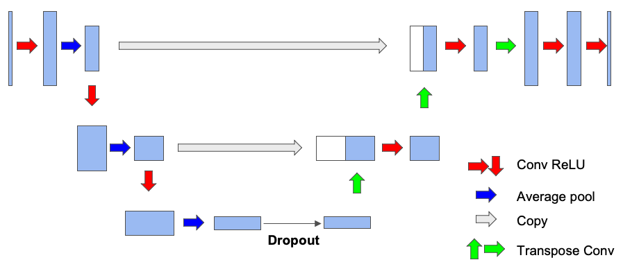
Fig. 1: Network architecture of our baseline ANN model.

3.1 Our proposed hybrid SNN fine-tuning

Inspired by a previous work on image classification network [9], we develop a hybrid SNN fine-tuning scheme for our segmentation network. We first train an ANN to its full convergence and then convert it to a spiking network with reduced time steps. The converted SNN is then taken as an initial state for a fine-tuning procedure.

The SNN neuron model in our work is integrate-and-fire (IF) model where the membrane potential will not decrease during the time when neuron does not fire as opposed to LIF neurons. The dynamics of our IF neurons can be described as:

$$u_{i}^{t}=u_{i}^{t-1}+\sum_{j}w_{ij}o_{j}-vo_{i}^{t-1}$$ (1)

$$o_{i}^{t-1}=\begin{cases}1&\textrm{if }u_{i}^{t-1}>v\\ 0&\textrm{otherwise}\end{cases}$$ (2)

where $u$ is the membrane potential, $t$ is the time step, subscript $i$ and $j$ represent the post- and pre-neuron, respectively,$w$ is the weight connecting the pre- and post-neuron, $o$ is the binary output spike, and $v$ is the firing threshold. Each neuron integrates the inputs from the previous layer into its membrane potential, and reduces the potential by a threshold voltage if a spike is fired.

Our SNN network has the same architecture as the baseline ANN, where the signals transmitted within the SNN are rate-coded spike trains generated through a Poisson generator. During the conversion process, we load the weights of the trained ANN into the SNN network and set the thresholds for all layers to 1s. Then a threshold balancing procedure [7] is carried out to update the threshold of each layer.

Fine-tuning of the converted SNN is conducted using spike-based backpropagation. It starts at the output layer, where the signals are continuous membrane potentials, generated through the summation:

$$u_{i}^{t}=u_{i}^{t-1}+\sum_{j}w_{ij}o_{j}$$ (3)

The number of neurons in the output layer is the same as the size of the input image. Compared with the hidden layer neurons in Eqn. 1, the output layer does not fire and therefore the voltage reduction term is removed. Each neuron in the output layer is connected to a Sigmoid activation function to produce the predictive probability of the corresponding pixel belonging to the target area (hippocampus).

Let $L(\cdot)$ be the loss function defined based on the ground-truth mask and the predictions. In the output layer, neurons do not generate spikes and thus do not have the non-differentiable problem. The update of the hidden layer parameters $W_{ij}$ is described by:

$$\Delta W_{ij}=\sum_{t}\frac{\partial L}{\partial W_{ij}^{t}}=\sum_{t}\frac{\partial L}{\partial o_{i}^{t}}\frac{\partial o_{i}^{t}}{\partial u_{i}^{t}}\frac{\partial u_{i}^{t}}{\partial W_{ij}^{t}}$$ (4)

Due to the non-differentiability of spikes, a surrogate gradient-based method is used in backpropagation. In [9], the authors propose a surrogate gradient function $\frac{\partial o^{t}}{\partial u^{t}}=\alpha e^{-\beta\Delta t}$. In this work, we choose a linear approximation proposed in [27], which is described as:

$$\frac{\partial o^{t}}{\partial u^{t}}=\alpha\max\{0,1-\left|u^{t}-V_{t}\right|\}$$ (5)

where $V_{t}$ is the threshold potential at time $t$, and $\alpha$ is a constant.

Our conversion + fine-tuning follows the same framework proposed in [9], which demonstrates that such hybrid approach can achieve, with much fewer time steps, similar accuracy compared to purely converted SNNs, as well as faster convergence than direct training methods. It should be noted that our work is the first attempt of exploring the application of spike-based fine-tuning and threshold balancing on fully convolutional networks (FCNs), including the U-Net.

3.2 Different losses

We explore different loss functions in this work, which include binary cross entropy (BCE), Dice loss and a combination of the two losses (BCE-Dice). BCE loss is the average of per-pixel loss and gives an unbiased measurement of pixel-wise similarity between prediction and ground-truth:

$$L_{\textrm{BCE}}=\sum_{i=1}^{N}-[r_{i}\log s_{i}+(1-r_{i})\log(1-s_{i})]$$ (6)

where $s_{i}\in[0,1]$ is the predicted value of a pixel and $r_{i}\in\{0,1\}$ is the ground-truth label for the same pixel. $\epsilon$ is a small number to smooth the loss, which is set to $10^{-5}$ in our experiments. Dice loss focuses more on the extent to which the predicted and ground-truth overlap:

$$L_{\textrm{Dice}}=\frac{2\sum_{i}s_{i}r_{i}+\epsilon}{\sum_{i}s_{i}+\sum_{i}r_{i}+\epsilon}$$ (7)

We also explore the effects of a weighted combination of BCE and Dice: $L_{\textrm{BCE\_Dice}}=0.3\times L_{\textrm{BCE}}+0.7\times L_{\textrm{Dice}}$

4 Experiments and Results

The data used in this work were obtained from the ADNI database (https://adni.loni.usc.edu/). In total, 110 baseline T1-weighted whole brain MRI images from different subjects along with their hippocampus masks were downloaded. In our experiments we only included normal control subjects. Due to the fact that the hippocampus only occupies a very small part of the whole brain and its position in the whole brain is relatively fixed, we roughly cropped the right hippocampus of each subject and use them as the input for segmentation. The size of the cropping box is $24\times 56\times 48$.

4.1 Training and testing

We train and evaluate our proposed model using a 5-fold cross-validation, with 22 and 88 subjects in the test and training sets, respectively, in each fold. The batch size in training and testing of ANN and SNN is set to 26. Training of both ANN and the SNN networks uses the Adam optimizer with slightly different parameters. The learning rate for training both networks is initially set to 0.001 and is later adjusted by the ReduceLROnPlateau scheduler in PyTorch, which monitors the loss during training, and tunes down the learning rate when it finds the loss stops dropping. Following a similar setup in [9], we use time steps of 200 for the ANN-SNN conversion routine. The ANN models were trained with 100 epochs and SNN models were trained over 35 epochs. Also, we repeat the ANN $\rightarrow$ Conversion $\rightarrow$ Fine-tuning procedure with three different loss functions: BCE only, Dice only and combined BCE and Dice.

4.2 Results

In this section, we present and evaluate the experimental results for the proposed model. Two different performance metrics, 3D Dice ratio and 2D slice-wise Dice ratio, were used to measure the accuracy of the segmentation models. The 3D Dice ratio was calculated subject-wise for each 3D volume. Mean and standard deviation averaged from 5 folds are reported. The 2D slice based Dice ratio was calculated slice by slice, and the mean and standard deviation were averaged from all test subjects’ slices.

Accuracies of the model on the test data are summarized in Table 1. The best performance for the ANN and fine-tuned SNN are highlighted with bold font. It is evident that network accuracies drop significantly after conversion (middle column) and our fine-tuning procedure can bring the performance of SNNs (right column) back close to the ANN level. The models built on the three loss functions have comparable performance in ANNs and fine-tuned SNNs, with Dice loss has slight edge over BCE and BCE-Dice combined.

Most fine-tuning procedures converge much faster than the maximal 35 epochs. On average, the three models in our experiments take 10.11 epochs to converge (with a standard deviation of 4.90). This achieves a great reduction in training complexity compared to the direct training models, which take roughly 60 epochs on average.

Loss	ANN Accuracy		Converted-SNN Accuracy		Fine-tuned SNN Accuracy
	2D	3D	2D	3D	2D	3D
BCE	$77.76\pm 2.40$	$83.17\pm 1.44$	$30.51\pm 9.93$	$21.60\pm 12.39$	$76.92\pm 3.77$	$81.83\pm 2.99$
Dice	${\bf 78.86\pm 2.39}$	${\bf 84.21\pm 1.66}$	$61.78\pm 3.32$	$65.90\pm 6.94$	${\bf 78.09\pm 3.85}$	$81.86\pm 4.40$
BCE-Dice	$78.58\pm 2.44$	$83.14\pm 1.59$	$52.03\pm 9.91$	$52.78\pm 14.73$	$77.72\pm 3.69$	${\bf 81.95\pm 3.24}$

Table 1: Average accuracies of ANNs, converted SNNs and fine-tuned SNNs built on three difference loss functions.

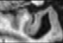
(a) Input slice

(b) Ground-truth mask

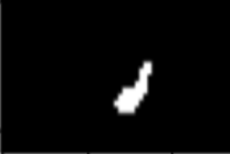
(c) Converted SNN

(d) Fine-tuned SNN

Fig. 2: An example slice of (a) input; (b) ground-truth mask; (c) segmentation result from the converted SNN; and (d) result from the fine-tuned SNN.

In order to find out how the fine-tuning procedure improves the segmentation accuracy, we look into details of both the outputs and the internal spiking patterns of the networks. Fig. 2 shows an example of input slice, ground-truth mask and the corresponding outputs from the converted and fine-tuned SNNs. We can see the output mask from the converted SNN (Fig. 2.(c)), while carrying a similar shape, is much smaller than the ground-truth. We believe the reason is that many neurons are not sufficiently activated due to the suboptimal thresholds set by the conversion procedure. The proposed fine-tuning step, on the other hand, can update the network weights to adjust for such thresholds, bringing the neurons back to active for improved accuracy. To confirm this thought, we record the firing frequency of each layer in the SNN models before and after the fine-tuning and plot them in Fig. 3. It is evident that neurons become more active after the fine-tuning, producing more accurate segmentation predictions.

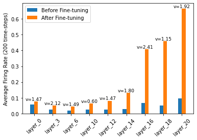
Fig. 3: Firing frequencies of neurons in different layers. Blue bars show those for a converted-SNN and orange bars are for the fine-tuned SNN. $v$ is the layer threshold.

5 Conclusions

In this work, we present a hybrid ANN-SNN fine-tuning scheme for the image segmentation problem. Our approach is rather general and can potentially be applied to many applications based on U-shaped networks. We take the human hippocampus as the target structure, and demonstrate the effectiveness of our approach through experiments on ADNI data. Exploring more applications is among our next steps.

References

- [1] Kaushik Roy, Akhilesh Jaiswal, and Priyadarshini Panda, “Towards spike-based machine intelligence with neuromorphic computing,” Nature, vol. 575, no. 7784, pp. 607–617, 2019.
- [2] Mike Davies, Andreas Wild, Garrick Orchard, Yulia Sandamirskaya, Gabriel A Fonseca Guerra, Prasad Joshi, Philipp Plank, and Sumedh R Risbud, “Advancing neuromorphic computing with loihi: A survey of results and outlook,” Proceedings of the IEEE, vol. 109, no. 5, pp. 911–934, 2021.
- [3] Alex Vicente-Sola, Davide L Manna, Paul Kirkland, Gaetano Di Caterina, and Trevor Bihl, “Keys to accurate feature extraction using residual spiking neural networks,” Neuromorphic Computing and Engineering, vol. 2, no. 4, pp. 044001, 2022.
- [4] Davide Liberato Manna, Alex Vicente-Sola, Paul Kirkland, Trevor Bihl, and Gaetano Di Caterina, “Simple and complex spiking neurons: perspectives and analysis in a simple stdp scenario,” Neuromorphic Computing and Engineering, 2022.
- [5] Peter U. Diehl, Daniel Neil, Jonathan Binas, Matthew Cook, Shih-Chii Liu, and Michael Pfeiffer, “Fast-classifying, high-accuracy spiking deep networks through weight and threshold balancing,” pp. 1–8, 2015.
- [6] Bodo Rueckauer, Iulia-Alexandra Lungu, Yuhuang Hu, and Michael Pfeiffer, “Theory and tools for the conversion of analog to spiking convolutional neural networks,” arXiv preprint arXiv:1612.04052, 2016.
- [7] Abhronil Sengupta, Yuting Ye, Robert Wang, Chiao Liu, and Kaushik Roy, “Going deeper in spiking neural networks: Vgg and residual architectures,” Frontiers in Neuroscience, vol. 13, 2019.
- [8] Nguyen-Dong Ho and Ik-Joon Chang, “Tcl: an ann-to-snn conversion with trainable clipping layers,” in 2021 58th ACM/IEEE Design Automation Conference (DAC). IEEE, 2021, pp. 793–798.
- [9] Nitin Rathi, Gopalakrishnan Srinivasan, Priyadarshini Panda, and Kaushik Roy, “Enabling deep spiking neural networks with hybrid conversion and spike timing dependent backpropagation,” 2020.
- [10] Sumit B Shrestha and Garrick Orchard, “Slayer: Spike layer error reassignment in time,” Advances in neural information processing systems, vol. 31, 2018.
- [11] Yujie Wu, Lei Deng, Guoqi Li, Jun Zhu, and Luping Shi, “Spatio-temporal backpropagation for training high-performance spiking neural networks,” Frontiers in neuroscience, vol. 12, pp. 331, 2018.
- [12] Yuhang Li, Yufei Guo, Shanghang Zhang, Shikuang Deng, Yongqing Hai, and Shi Gu, “Differentiable spike: Rethinking gradient-descent for training spiking neural networks,” Advances in Neural Information Processing Systems, vol. 34, pp. 23426–23439, 2021.
- [13] Youngeun Kim, Joshua Chough, and Priyadarshini Panda, “Beyond classification: directly training spiking neural networks for semantic segmentation,” arXiv preprint arXiv:2110.07742, 2021.
- [14] Kinjal Patel, Eric Hunsberger, Sean Batir, and Chris Eliasmith, “A spiking neural network for image segmentation,” arXiv preprint arXiv:2106.08921, 2021.
- [15] Kevin H Hobbs, Pin Zhang, Bibo Shi, Charles D Smith, and Jundong Liu, “Quad-mesh based radial distance biomarkers for alzheimer’s disease,” in 2016 ISBI. IEEE, 2016, pp. 19–23.
- [16] Bibo Shi, Yani Chen, Pin Zhang, Charles D Smith, Jundong Liu, et al., “Nonlinear feature transformation and deep fusion for alzheimer’s disease staging analysis,” Pattern recognition, vol. 63, pp. 487–498, 2017.
- [17] Olaf Ronneberger, Philipp Fischer, and Thomas Brox, “U-net: Convolutional networks for biomedical image segmentation,” in International Conference on Medical image computing and computer-assisted intervention. Springer, 2015, pp. 234–241.
- [18] Pierrick Coupé, José V Manjón, Vladimir Fonov, Jens Pruessner, Montserrat Robles, and D Louis Collins, “Patch-based segmentation using expert priors: Application to hippocampus and ventricle segmentation,” NeuroImage, vol. 54, no. 2, pp. 940–954, 2011.
- [19] Tong Tong, Robin Wolz, Pierrick Coupé, Joseph V Hajnal, Daniel Rueckert, et al., “Segmentation of mr images via discriminative dictionary learning and sparse coding: Application to hippocampus labeling,” NeuroImage, vol. 76, pp. 11–23, 2013.
- [20] Yantao Song, Guorong Wu, Quansen Sun, Khosro Bahrami, Chunming Li, and Dinggang Shen, “Progressive label fusion framework for multi-atlas segmentation by dictionary evolution,” in MICCAI. Springer, 2015, pp. 190–197.
- [21] Yani Chen, Bibo Shi, Zhewei Wang, Tao Sun, Charles D Smith, and Jundong Liu, “Accurate and consistent hippocampus segmentation through convolutional lstm and view ensemble,” in MLMI 2017. Springer, 2017, pp. 88–96.
- [22] Yani Chen, Bibo Shi, Zhewei Wang, Pin Zhang, Charles D Smith, and Jundong Liu, “Hippocampus segmentation through multi-view ensemble convnets,” in ISBI 2017. IEEE, 2017, pp. 192–196.
- [23] Youngeun Kim and Priyadarshini Panda, “Revisiting batch normalization for training low-latency deep spiking neural networks from scratch,” Frontiers in neuroscience, p. 1638, 2020.
- [24] Qianhui Liu, Gang Pan, Haibo Ruan, Dong Xing, Qi Xu, and Huajin Tang, “Unsupervised aer object recognition based on multiscale spatio-temporal features and spiking neurons,” IEEE TNNLS, vol. 31, no. 12, pp. 5300–5311, 2020.
- [25] Eric Hunsberger and Chris Eliasmith, “Spiking deep networks with lif neurons,” arXiv preprint arXiv:1510.08829, 2015.
- [26] Daniel Rasmussen, “Nengodl: Combining deep learning and neuromorphic modelling methods,” Neuroinformatics, vol. 17, no. 4, pp. 611–628, 2019.
- [27] Guillaume Bellec, Darjan Salaj, Anand Subramoney, Robert Legenstein, and Wolfgang Maass, “Long short-term memory and learning-to-learn in networks of spiking neurons,” Advances in neural information processing systems, vol. 31, 2018.