Generalized parton distributions through universal moment parameterization: non-zero skewness case

Abstract

We present the first global analysis of generalized parton distributions (GPDs) combing lattice quantum chromodynamics (QCD) calculations and experiment measurements including global parton distribution functions (PDFs), form factors (FFs) and deeply virtual Compton scattering (DVCS) measurements. Following the previous work where we parameterize GPDs in terms of their moments, we extend the framework to allow for the global analysis at non-zero skewness. Together with the constraints at zero skewness, we fit GPDs to global DVCS measurements from both the recent JLab and the earlier Hadron-Electron Ring Accelerator (HERA) experiments with two active quark flavors and leading order QCD evolution. With certain choices of empirical constraints, both sea and valence quark distributions are extracted with the combined inputs, and we present the quark distributions in the proton correspondingly. We also discuss how to extend the framework to accommodate more off-forward constraints beyond the small $\xi$ expansion, especially the lattice calculated GPDs.

1 Introduction

Over the past two decades, there has been growing interest in the higher-dimensional structures of the nucleon in the studies of the non-perturbative strong interactions described by quantum chromodynamics (QCD). Consequently, generalized parton distributions (GPDs) Muller:1994ses ; Ji:1996ek ; Ji:1998pc that unify the elastic form factors (FFs) and Parton Distributions Functions (PDFs) into a single set of 3-dimensional (3D) functions and contain important information about the nucleon mass, angular momentum and mechanical properties Ji:1994av ; Ji:1996ek ; Polyakov:2002yz have gained increasing attention. While it is believed that GPDs can be experimentally accessed by exclusive productions of particles off nucleons such as deeply virtual Compton scattering (DVCS) Ji:1996nm and deeply virtual meson production (DVMP) Radyushkin:1996ru ; Collins:1996fb , obtaining them and the corresponding nucleon 3D structures from experimental data has remained a dream. On the one hand, persisting efforts are needed for an adequate amount of data as required for the extraction of such high-dimensional quantities. On the other hand, the extraction of the critical information from experimental data has also been challenging.

Several recent breakthroughs have made this possible. Large data sets of exclusive measurements are generated at Jefferson Lab (JLab) CLAS:2018ddh ; CLAS:2021gwi ; Georges:2017xjy ; JeffersonLabHallA:2022pnx , and more will come from the planned Electron-Ion Collider (EIC) Accardi:2012qut ; AbdulKhalek:2021gbh at Brookhaven National Lab (BNL). Additionally, novel developments in lattice QCD allow the access to the nucleon structures from first principle calculation Ji:2013dva ; Ji:2020ect ; Alexandrou:2020zbe ; Lin:2021brq , providing information almost impossible to get with current and future experiments. This recent progress, together with the perennial efforts on the global extraction of PDFs Hou:2019efy ; NNPDF:2021njg ; Ethier:2017zbq , FFs Ye:2017gyb as well as lattice calculation of generalized form factors Alexandrou:2021jok ; Hasan:2017wwt ; Shintani:2018ozy ; Jang:2018djx , have pushed the study of nucleon 3D structures to a new stage, which, on the other hand, requires extra works to put all the above inputs together through global analysis to obtain the state-of-art nucleon 3D structures with GPDs.

Therefore, we are in need of a global analysis program of GPDs with both experimental data and lattice computation. Lots of efforts are put into parameterizing and accessing GPDs from various inputs in the literature Polyakov:2002wz ; Guidal:2004nd ; Goloskokov:2005sd ; Mueller:2005ed ; Kumericki:2009uq ; Goldstein:2010gu ; Gonzalez-Hernandez:2012xap ; Kriesten:2021sqc ; Hashamipour:2021kes . However, a framework that could combine experimental data and lattice computation still seems to be lacking. In the previous work Guo:2022upw , we proposed the GPDs through universal moment parameterization (GUMP) program for such a purpose and studied the zero-skewness case as an illustrative example. In this work, we follow the previous setup and extend it to non-zero skewness, which allows us to also include the exclusive measurements in the global analysis. With such a program, we perform the global analysis of GPDs that includes global PDFs Hou:2019efy ; NNPDF:2021njg ; Ethier:2017zbq , FFs Ye:2017gyb and DVCS measurements from both JLab CLAS:2018ddh ; CLAS:2021gwi ; Georges:2017xjy ; JeffersonLabHallA:2022pnx and previous H1 H1:2009wnw experiments at Hadron-Electron Ring Accelerator (HERA) along with the relevant lattice calculations related to GPDs Alexandrou:2021jok ; Alexandrou:2020zbe for the first time.

The organization of the paper is as follows. In sec. 2, we introduce the setup for the GUMP program and discuss how to build the 3D GPDs with a handleable set of parameters. In sec. 3, we discuss more details of the fit and present the extracted Compton form factors (CFFs) and GPDs, where we also discuss how to extend the present framework to accommodate more future inputs. In the end, we conclude in sec. 4.

2 Conventions and fitting procedure

In the previous work Guo:2022upw , we discussed how GPDs can be parameterized in terms of their moments based on the technique that has been systematically developed in ref. Mueller:2005ed and used for instance in ref. Kumericki:2009uq . In this section, we will discuss how we apply such a framework to the GPDs at non-zero skewness, including GPDs of various different species and flavors.

2.1 Convention and decomposition of GPD

We start by considering the four leading-twist GPDs $H,E,\widetilde{H}$ and $\widetilde{E}$, where each of them has different flavors $u,d$ and $g$ corresponding to the up and down quarks as well as the gluon. Although the strange quark might have sizable effects that should be considered for a more careful treatment, the flavor separation of GPDs is typically challenging due to the lack of a flavor-sensitive probe Cuic:2020iwt . Strange quark distributions will not be well constrained with just DVCS measurements, and thus we will leave this for the future work with more flavor-sensitive measurements.

For simplicity, the four different species of GPDs will be treated almost equally in this work. Except that the vector GPDs $H$ and $E$ satisfy slightly different scale evolution equations from the axial-vector ones $\widetilde{H}$ and $\widetilde{E}$ Kumericki:2007sa , the same parameterization will be used for all four GPDs. Although GPDs or combinations of GPDs of different species $H,E,\widetilde{H}$ and $\widetilde{E}$ correspond to different helicity amplitudes and might have different behaviors accordingly, knowledge of different GPDs species is limited and thus implementing a different parameterization for them individually may not lead to any significant difference. Therefore, we collectively denote all GPDs as $F_{q,g}(x,\xi,t)$ where $F=\{H,E,\widetilde{H},\widetilde{E}\}$ and $q=\{u,d\}$, with $x$ the parton momentum fraction, $\xi$ the skewness parameter and $t$ the total momentum transfer squared and parameterize them in the same manner. We note that the skewness parameter $\xi$ generally takes the value from $-1$ to $1$, but it will be considered to be positive hereafter, as GPDs are commonly defined to be symmetric in $\xi$, subject to their parity symmetry.

An intriguing feature of the GPDs is that they consist of two regions with totally different physical interpretations. In the PDF-like region where $x>\xi$ or $x<-\xi$, GPDs resemble the PDFs which are interpreted as the amplitudes of emitting and reabsorbing a parton (quark, antiquark or gluon). On the other hand, in the distribution amplitude (DA)-like region where $-\xi<x<\xi$, they resemble the DAs instead and are interpreted as the amplitudes of emitting/absorbing a parton-antiparton pair. Therefore, GPDs do not naturally have distinguishable quark and antiquark components, especially in the DA-like region. This feature indicates that the parameterization of GPDs should be flexible in both the PDF and DA-like regions, since different physics are involved.

Motivated by such property, one can write GPDs as,

$$F_{q}(x,\xi,t)\equiv F_{\hat{q}}(x,\xi,t)\mp F_{\bar{q}}(-x,\xi,t)+F_{q\bar{q}}(x,\xi,t)\ ,$$ (1)

where the $\mp$ depends on the parity of the GPDs which takes $-$ for vector GPDs $H$ and $E$ and $+$ for axial vector GPDs $\widetilde{H}$ and $\widetilde{E}$. Here the subscript $\hat{q}$ stands for the quark distributions excluding antiquark, to be distinguished from the subscript $q$ for the quark flavor. The three terms above describe the amplitudes corresponding to the quark, antiquark, and quark-antiquark pair respectively. Accordingly, $F_{\hat{q}}(x,\xi,t)$ and $F_{\bar{q}}(x,\xi,t)$ have support $x>-\xi$, while the $F_{{q}\bar{q}}(x,\xi,t)$ has support $\xi>x>-\xi$. In the semi-forward limit where $\xi=0$ and $t$ generally non-zero, $F_{\hat{q}}(x,\xi,t)$ and $F_{\bar{q}}(x,\xi,t)$ reduce to the quark and antiquark $t$-dependent PDFs with support $x>0$, whereas $F_{{q}\bar{q}}(x,\xi,t)$ vanishes with its vanishing support. We note that GPDs can always be decomposed into such three parts that each term represents the behavior of GPDs in different regions respectively. The extra DA terms $F_{{q}\bar{q}}(x,\xi,t)$ allow extra flexibility for the parameterization of GPDs particularly in the DA-like region, as we will discuss with more details in the next section.

While the quark and antiquark GPDs $F_{\hat{q}}(x,\xi,t)$ and $F_{\bar{q}}(x,\xi,t)$ are the natural generalization of the quark and antiquark PDFs, the DA terms $F_{{q}\bar{q}}(x,\xi,t)$, also known as the $D$-terms in some other contexts Polyakov:1999gs , only exists in the off-forward case. Such terms live in the DA-like region only, and they will be the dominant effects in the large $\xi$ limit $\xi\to 1$ or the asymptotic limit where renormalization scale $\mu\to\infty$ Goeke:2001tz ; Diehl:2003ny . Since the DA terms vanish at the crossover line $x=\pm\xi$, they can always be expressed with a set of complete polynomials like Gegenbauer polynomials, which is exactly the conformal moment expansion. Therefore, each of the three terms can be expressed in terms of their conformal moments and satisfies the polynomiality condition.

In this work, we will focus on the quark and antiquark GPDs $F_{\hat{q}}(x,\xi,t)$ and $F_{\bar{q}}(x,\xi,t)$, whereas the extra DA terms $F_{q\bar{q}}(x,\xi,t)$ will not be put into the global analysis for two reasons. First, as discussed in the previous work, we will consider the high energy limit where $\xi\to 0$ ideally and the DA-like region disappears in such a limit. Second, since the DA terms vanish at the crossover line $x=\pm\xi$, they are hard to extract with measurements of DVCS or similar processes which provide effectively just CFFs — the DA terms contribute to the real part of the CFFs only, corresponding to the subtraction terms in the dispersion relations of CFFs Kumericki:2009uq . Consequently, the behaviors of GPDs in the DA-like region given by the quark and antiquark GPDs $F_{\hat{q}}(x,\xi,t)$ and $F_{\bar{q}}(-x,\xi,t)$ will be ambiguous, since one can add extra DA terms without affecting the CFFs too much in the small $\xi$ limit. This will be discussed with more details in the next section.

We note that another notation of quark and antiquark GPDs has been used in the literature, see for instance ref. Muller:2014wxa

$$\begin{split}F_{\hat{q}}(x>\xi,\xi,t)&=F_{q}(x,\xi,t)\ ,\\ F_{\bar{q}}(x>\xi,\xi,t)&=\mp F_{q}(-x,\xi,t)\ ,\end{split}$$ (2)

with the same convention for the $\mp$ sign. Since the quark and antiquark GPDs are defined with the same function $F_{q}(x,\xi,t)$ partitioned into two parts, the full quark GPD $F_{q}(x,\xi,t)$ cannot be written as the sum of them $F_{q}(x,\xi,t)\not=F_{\hat{q}}(x,\xi,t)\mp F_{\bar{q}}(-x,\xi,t)$. Due to the loss of linearity in such a GPD decomposition, which will also break the polynomiality condition for quark and antiquark GPDs respectively, this definition will not be used in this work.

To summarize, we will consider quark and antiquark GPDs $F_{\hat{q}}(x,\xi,t)$, $F_{\bar{q}}(x,\xi,t)$ as well as the gluon GPDs $F_{g}(x,\xi,t)$ in this work with four twist-two GPDs $H,E,\widetilde{H}$ and $\widetilde{E}$, forming a basis with 20 GPDs. Conventionally, we also rewrite the basis by defining the valence combination: $F_{q_{V}}(x,\xi,t)\equiv F_{\hat{q}}(x,\xi,t)-F_{\bar{q}}(x,\xi,t)$, and thus the basis can be written with $F_{q_{V}}(x,\xi,t)$, $F_{\bar{q}}(x,\xi,t)$ and $F_{g}(x,\xi,t)$ equivalently, analogous to the basis commonly chosen for PDFs global analysis in the literature Hou:2019efy ; NNPDF:2021njg ; Ethier:2017zbq .

2.2 Parameterization of moments

After introducing the GPDs necessary for consideration, we briefly discuss the parameterization method for GPDs. We have introduced the GUMP parameterization in the previous work Guo:2022upw and more about the conformal moment representation can be found in refs. Mueller:2005ed ; Kumericki:2009uq . Generally, we express all GPDs $F(x,\xi,t)$ in terms of their conformal moments $\mathcal{F}_{j}(\xi,t)$ in the form of,

$$F(x,\xi,t)=\sum_{j=0}^{\infty}(-1)^{j}p_{j}(x,\xi)\mathcal{F}_{j}(\xi,t)\quad\text{for }|x|<\xi\ ,$$ (3)

with $p_{j}(x,\xi)$ the known conformal wave functions. Therefore, all GPDs $F(x,\xi,t)$ are equivalently given by $\mathcal{F}_{j}(\xi,t)$. With the polynomiality condition of GPDs Ji:1998pc , the moments can be expressed as polynomials of $\xi$ of given order:

$$\mathcal{F}_{j}(\xi,t)=\sum_{k=0,\rm{even}}^{j+1}\xi^{k}\mathcal{F}_{j,k}(t)\ ,$$ (4)

and then these $\mathcal{F}_{j,k}(t)$ can be used to construct the GPD $F(x,\xi,t)$.

In the high energy limit, the skewness parameter $\xi=x_{B}/(2-x_{B})+\mathcal{O}(Q^{-2})$ is small where the first few terms dominate, and we have Kumericki:2009uq

$$\mathcal{F}_{j}(\xi,t)=\mathcal{F}_{j,0}(t)+\xi^{2}\mathcal{F}_{j,2}(t)+\mathcal{O}(\xi^{4})\ ,$$ (5)

where we implicitly assume that the $\mathcal{F}_{j,k}(t)$ are only non-zero for $j>k$ according to the polynomiality condition. Practically the moments $\mathcal{F}_{j,k}(t)$ can be written in terms of the shape governed by the Euler beta function $B$, the Regge trajectory for the $t$-dependence and the extra residual term $\beta(t)$:

$$\mathcal{F}_{j,k}(t)=\sum_{i=1}^{i_{\rm{max}}}N_{i,k}B(j+1-\alpha_{i,k},1+\beta_{i,k})\frac{j+1-k-\alpha_{i,k}}{j+1-k-\alpha_{i,k}(t)}\beta(t)\ ,$$ (6)

with which the GPDs are parameterized in terms of the free parameters in eq. (6). In the simplest case, only one set of ansatz is needed, so we set $i_{\rm{max}}$ to be just $1$.

In the previous work, we simply set the residual function $\beta(t)$ to be 1 for the extraction of valence quark distributions in the zero-skewness case, since their algebraic decaying behaviors in $|t|$ can be parameterized well by the Regge trajectory. However, for the sea distributions, it has been observed that in high energy processes, the different cross-sections drop exponentially as the momentum transfer $|t|$ increases e.g., for DVCS H1:2007vrx ; H1:2009wnw , which differs from the power-law behavior indicated by the Regge theory. Therefore, we incorporate the extra exponential behavior into the $\beta(t)$ to set $\beta(t)=\exp(bt)$. Two $\beta(t)$s of different $b$ slope are embedded in the parameterization of the vector GPDs $H_{\bar{q},g}$ and the axial vector GPDs $\widetilde{H}_{\bar{q},g}$ respectively, with $q=\{u,d\}$ for sea quarks. We note that due to the lack of flavor-sensitive probe, we assume the same $b$ slope for the gluon and sea quarks of different flavor and also the same Regge slope $\alpha^{\prime}$ for them which is fixed to be $\alpha^{\prime}_{\bar{q},g}=0.15$ from the pomeron trajectory H1:2005dtp .

Even with such simplification, the parameters are still too many to be fully determined from measurements. The lack of off-forward constraints makes it almost impossible to get the shape of GPDs at non-zero skewness, which is known as the deconvolution problem of GPDs Bertone:2021yyz , stating that the shape of GPDs can not be uniquely determined from CFFs. Therefore, extra empirical constraints are still needed for the extraction of GPDs. The simplest choice for the $\xi$-dependent terms is to set them to be proportional to the leading terms, as has been done in ref. Kumericki:2009uq :

$$\mathcal{F}_{j,k}(t)=R_{k}\mathcal{F}_{j-k,0}(t)\ ,$$ (7)

with $R_{k}$ the ratio between them. In this work, we have just one parameter $R_{2}$ for the $\xi^{2}$ terms for each GPD $F(x,\xi,t)$ that accounts for its extra $\xi$-dependence.

Another difficulty in GPD parameterization is about the flavors and species of GPDs. While the extraction of one 3D function is already challenging, the simultaneous extraction of GPDs with multiple flavors and species is yet more difficult. Two of the four different species of GPDs, $E$ and $\widetilde{E}$, do not have corresponding forward PDFs, unlike $H$ and $\widetilde{H}$ which reduce to the PDF $f(x)$ and helicity PDF $\Delta f(x)$ respectively, adding extra difficulties to their extraction. Consequently, we have to reduce the number of parameters associated to these two GPDs due to the lack of constraints. To do so, we set the two valence quark distributions to be proportional ($E_{u_{V}}\propto E_{d_{V}}$ and $\widetilde{E}_{u_{V}}\propto\widetilde{E}_{d_{V}}$) and the sea quark as well as the gluon distributions to be proportional to the corresponding $H$ and $\widetilde{H}$ GPDs.

We note that these extra empirical constraints, both for the $\xi$-dependent terms and for the $E/\widetilde{E}$ GPDs, are added for purely practical purposes. As mentioned above, they simply represent the lack of information of GPDs in the off-forward region, which can and should be improved in the future with more inputs from both lattice calculations and experimental measurements. In table 1, we collect whether GPDs of different species and flavors are either parameterized independently with eq. (6) or linked to the other GPDs with some empirical assumptions in this work.

GPDs species and flavors	Fully parameterized	GPDs linked to	Proportional constants
$H_{u_{V}}$ and $\widetilde{H}_{u_{V}}$	✔	-	-
$E_{u_{V}}$ and $\widetilde{E}_{u_{V}}$	✔	-	-
$H_{d_{V}}$ and $\widetilde{H}_{d_{V}}$	✔	-	-
$E_{d_{V}}$ and $\widetilde{E}_{d_{V}}$	✘	$E_{u_{V}}$ and $\widetilde{E}_{u_{V}}$	$R^{E/\widetilde{E}}_{d_{V}}$
$H_{\bar{u}}$ and $\widetilde{H}_{\bar{u}}$	✔	-	-
$E_{\bar{u}}$ and $\widetilde{E}_{\bar{u}}$	✘	$H_{\bar{u}}$ and $\widetilde{H}_{\bar{u}}$	$R^{E/\widetilde{E}}_{\rm{sea}}$
$H_{\bar{d}}$ and $\widetilde{H}_{\bar{d}}$	✔	-	-
$E_{\bar{d}}$ and $\widetilde{E}_{\bar{d}}$	✘	$H_{\bar{d}}$ and $\widetilde{H}_{\bar{d}}$	$R^{E/\widetilde{E}}_{\rm{sea}}$
$H_{g}$ and $\widetilde{H}_{g}$	✔	-	-
$E_{g}$ and $\widetilde{E}_{g}$	✘	$H_{g}$ and $\widetilde{H}_{g}$	$R^{E/\widetilde{E}}_{\rm{sea}}$

Table 1: A summary of how each GPDs with different species and flavors are parameterized respectively. Fully parameterized GPDs are expressed in terms of eq. (6), whereas the other GPDs are linked to the fully parameterized GPDs with proportional constants.

Finally, we comment on the comparison of the GUMP program to the other GPD global analysis programs with conform moments framework, specifically the Kumerički-Müller (KM) model and its extensions Kumericki:2007sa ; Kumericki:2009uq ; Muller:2013jur ; Mueller:2014hsa . As clearly stated in the previous work Guo:2022upw , the GUMP program follows the general conformal moment parameterization of GPDs, and adopts many useful observations there to make the GUMP parameterization practical. On the other hand, this program focuses more on the extraction of all four leading-twist GPDs including both valence and sea quarks of different flavors with the combined inputs from both lattice calculations and experiments. Therefore, though in a similar spirit, the GUMP program allows a more comprehensive study of the GPDs, especially the valence parts which are effectively constrained by lattice calculations while less accessible from experiments.

2.3 Inputs and fitting strategy

With the above parameterization, the global analysis can be performed with adequate inputs to pin down all the parameters. In this subsection, we will discuss how we select inputs from all the available results for the global analysis.

We start with the forward inputs where GPDs reduce to PDFs. While we could have various inclusive measurements as the inputs rather than the global PDFs extracted from a specific work to avoid the bias, there are several reasons we choose the extracted PDFs for the GPD global analysis. First, the extraction of the PDFs themselves is considerably involved and requires dedicated works, especially for the simultaneous extraction of both unpolarized and polarized PDFs Cocuzza:2022jye ; Zhou:2022wzm . Second, much less is known for the off-forward behaviors of GPDs compared to the forward ones. Consequently, a fine forward analysis can not be matched with an equivalent off-forward analysis, making it less urgent to improve the forward part of the analysis. Therefore, we avoid repeating the forward fittings that have been studied extensively by the PDF global analysis community and take their globally extracted PDFs as the inputs. More specially, we consider one of the recent analyses by the JAM collaboration  Cocuzza:2022jye , where both the unpolarized and polarized proton PDFs are extracted simultaneously.

The off-forward inputs, on the other hand, consist of various constraints including globally extracted FFs Ye:2017gyb , lattice calculations Alexandrou:2021jok ; Alexandrou:2020zbe and exclusive measurements, or the DVCS measurements CLAS:2018ddh ; CLAS:2021gwi ; Georges:2017xjy ; JeffersonLabHallA:2022pnx ; H1:2009wnw more specifically for this work. For the form factors, we take the globally extracted charge FFs Ye:2017gyb rather than fit to the elastic scattering data directly Hashamipour:2021kes for the same reasons as for the PDFs. Since the charge form factors are averaged over all flavors, we combine the charge form factors of both proton and neutron to obtain the charge form factors of up and down quarks respectively, assuming isospin symmetry and ignoring the contributions of strange and other heavy flavors.

The lattice inputs include both calculations of generalized form factors and $x$-dependence of GPDs Alexandrou:2021jok ; Alexandrou:2020zbe . Putting the lattice QCD results together with other experimental measurements can be quite subtle, due to the systematic uncertainties of the lattice results that are hard to fully understand. Progress has been made in getting the systematic uncertainties under control and calculations from different groups are converging for certain quantities like the (axial) charge form factors, see for instance the review in ref. Constantinou:2020hdm , but more efforts are still in demand to get the other results consistent. Therefore, in this work we consider the lattice results from a single group only Alexandrou:2021jok ; Alexandrou:2020zbe to avoid the potential tension among lattice results from different groups. On the other hand, we adjust their weights in the global analysis by increasing the uncertainties of the results to account for the unknown systematic uncertainties. We note that the calculation of the $x$-dependence of GPDs at non-zero skewness has been done in the literature Alexandrou:2020zbe , although the reliable regions with controlled systematic uncertainties get even more subtle due to the irregular behavior of GPDs at $x=\xi$. Thus, the inclusion of the $x$-dependence of GPDs at non-zero skewness in the global analysis will be left to the future work.

Last but not the least, we have the experimental exclusive measurements. In principle, the exclusive measurements can and should include as many processes as possible to get better constraints on the GPDs as well as to test the universality of GPDs. However, the main challenge for putting different processes together is the mismatch in the amount of data available. Two types of Compton scattering processes, DVCS and Time-like Compton Scattering (TCS) Berger:2001xd , have been measured at JLab. Much more DVCS data have been obtained than that of TCS, of which the first measurement was made just recently CLAS:2021lky . On the other hand, DVMP typically requires much larger virtuality than DVCS to suppress the unwanted contributions of transverse polarization, which are mostly accessible with colliders such as HERA ZEUS:2005bhf ; H1:2005dtp and the future EIC Accardi:2012qut ; AbdulKhalek:2021gbh . Therefore, we start by considering the DVCS measurements only, which has the broadest global kinematical coverage among these process that includes both the low $x_{B}$ region covered by H1 H1:2009wnw at HERA and the medium $x_{B}$ region covered by various experiments at JLab CLAS:2018ddh ; CLAS:2021gwi ; Georges:2017xjy ; JeffersonLabHallA:2022pnx . It is worth noting that the DVCS process is mostly sensitive to the quark distributions whereas the gluon distributions are best obtained from meson production or other gluon-sensitive processes. Obtaining the gluonic distributions from them is indeed of high interest and importance, which will be carried out in a separate work.

With all the inputs above, it seems straightforward to simply put them together and perform the global analysis with the parameterization described before. However, it will not be quite practical with the large number of free parameters, which typically means extremely slow convergence in the search of best-fit parameters. Besides, the evaluation of GPDs, especially with scale evolution, is much more computationally intensive, compared to that of the PDFs for instance, making the global analysis even less handleable. Therefore, we split the global analysis into two steps by first performing the semi-forward fit at zero skewness $\xi=0$ (while the momentum transfer squared $t$ can still be non-zero) and then fit to the off-forward inputs with non-zero skewness $\xi\not=0$. Apparently, the two-step fitting introduces bias that favors the semi-forward constraints over the off-forward constraints. However, given the fact that much more semi-forward constraints can be obtained from lattice and experiments than the off-forwards ones, it is a reasonable and practical assumption for such a large system of parameters.

3 Global analysis and extracted GPDs

In the previous section, we discussed the parameterization of GPDs as well as the inputs to constrain the parameters, so we would need to find the set of parameters that fit to the measurements best, for which we employ the iminuit interface of Minuit2 iminuit ; James:1975dr as the minimizer. In this section, we will present the results of the global analysis as well as the extracted CFFs and GPDs.

3.1 Basics of the fit

As discussed before, the whole fit will be split into the semi-forward ($\xi=0$) part and the off-forward ($\xi\not=0$) part to avoiding dealing with the huge parameter set in a single fit. Furthermore, in the semi-forward case constraints on different species $H$, $E$, $\widetilde{H}$, and $\widetilde{E}$ decouple, unlike the off-forward case where all four of them are involved. This allows one to further decompose the semi-forward fit into four separate fits that do not interfere for each of the four $t$-dependent PDFs. Therefore, the whole fitting procedure eventually consists of five individual fits as shown in figure 1. Correspondingly, the total $\chi^{2}$ can be decomposed into five parts:

$$\chi^{2}_{\text{tot}}=\chi^{2}_{\text{fwd}}+\chi^{2}_{\text{off-fwd}}=\chi^{2}_{H}+\chi^{2}_{E}+\chi^{2}_{\widetilde{H}}+\chi^{2}_{\widetilde{E}}+\chi^{2}_{\text{off-fwd}}\ ,$$ (8)

where each term $\chi^{2}_{F}$ with $F=\{H,E,\widetilde{H},\widetilde{E}\}$ stands for the $\chi^{2}$ for the semi-forward fits of the corresponding $t$-dependent PDFs. Then one just needs to minimize these $\chi^{2}$s separately in order to perform the fit and the results are summarized in table 2. More details of the fitted parameters are presented in Appendix A.

Figure 1: A plot showing the fitting procedure of the GUMP program. The semi-forward ($\xi=0$) fit that consists of four individual fits for each $t$-dependent PDF is performed before the off-forward ($\xi\not=0$) fit. The results of the semi-forward fit are then passed to the off-forward fit as fixed parameters, whereas the off-forward parameters will be determined with the off-forward constraints.

Sub-fits	$\chi^{2}$	$N_{\text{data}}$	$\chi^{2}_{\nu}\equiv\chi^{2}/\nu$
Semi-forward
$t$PDF $H$	281.7	217	1.41
$t$PDF $E$	59.7	50	1.36
$t$PDF $\widetilde{H}$	159.3	206	0.84
$t$PDF $\widetilde{E}$	63.8	58	1.23
Off-forward
JLab DVCS	1413.7	926	$\sim$ 1.53
H1 DVCS	19.7	24	$\sim$ 0.82
Off-forward total	1433	950	1.53
Total	2042	1481	1.40

Table 2: A table summarizing the total $\chi^{2}$ versus the number of data points $N_{\text{data}}$ as well as the $\chi^{2}$ per degree of freedom $\chi^{2}_{\nu}$. Since the JLab and H1 DVCS measurements are fitted simultaneously in the off-forward fit, the $\chi^{2}/\nu$ is replaced with $\chi^{2}/N_{\text{data}}$ instead to estimate their separate contributions.

Several comments are as follows: first, we take the globally fitted unpolarized and polarized PDFs Cocuzza:2022jye with 31 points sampled in the region $x\in[0.005,0.6]$ for each flavor, indicating 155 points for the $t$-dependent PDFs $H$ and $\widetilde{H}$ respectively. Note that since the parameterization we used has only 3 parameters in the forward limit for each PDF, much less than the PDF global analysis Hou:2019efy , the sample size can not be too large correspondingly. The extra constraints from PDFs on $H$ and $\widetilde{H}$ account for their larger $N_{\rm{data}}$ as shown in table 2, while the other around 50 data for each $t$-dependent PDF are taken from the globally fitted FFs Ye:2017gyb and lattice calculations Alexandrou:2021jok ; Alexandrou:2020zbe .

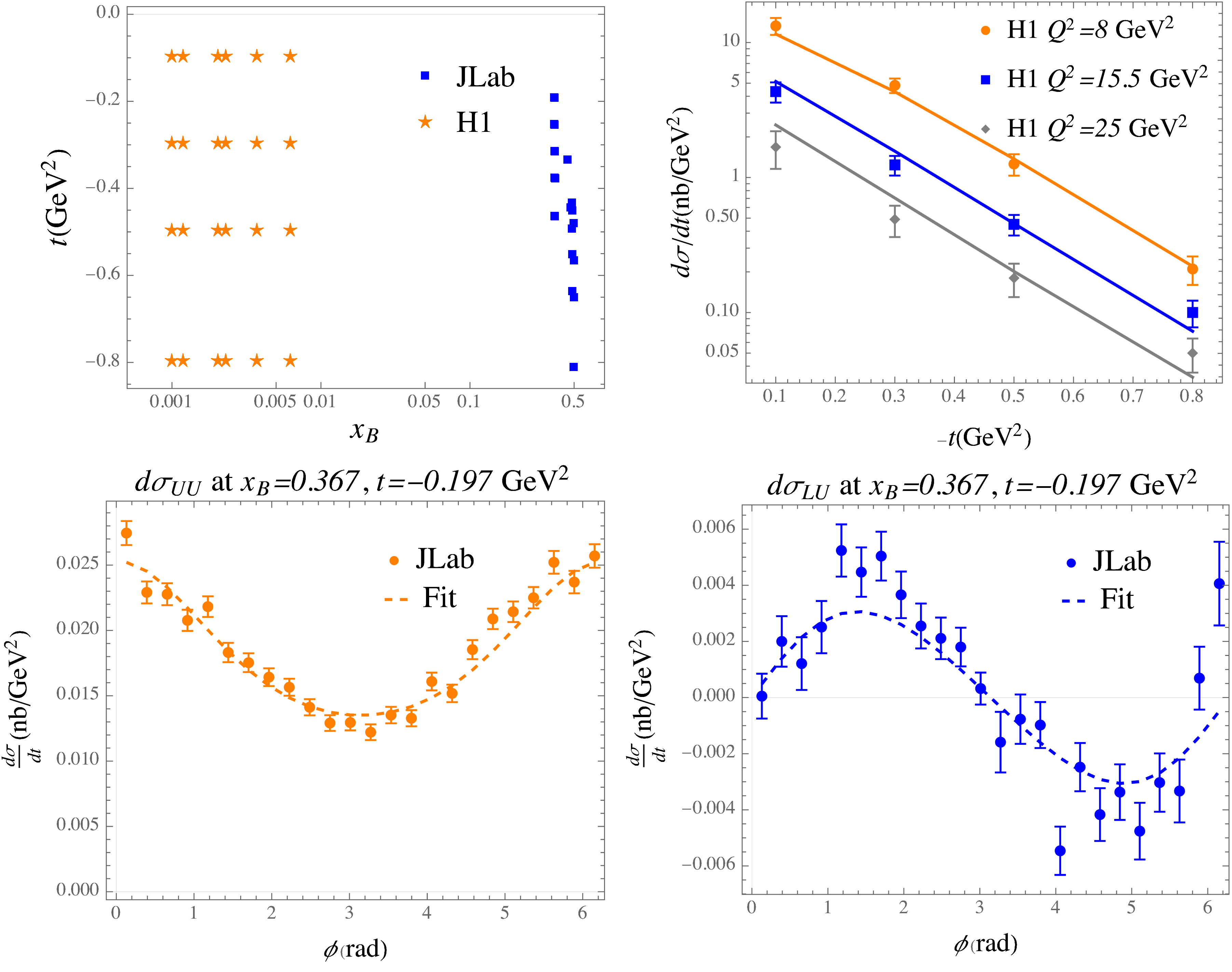
Figure 2: The top left panel shows the kinematical coverage of the DVCS measurements including both JLab and H1. The top-right panel shows the fit to the DVCS measurements at H1 with the azimuthal angel $\phi$ integrated, whereas the lower two figures show examples of the fit to the JLab DVCS cross-section measurements at $Q^{2}=3.65\text{ GeV}^{2}$ in the azimuthal angel $\phi$ for both polarized and unpolarized beam. Contributions of Bethe-Heitler process are calculated with the electromagnetic form factors in ref. Ye:2017gyb . The DVCS and interference cross-sections are calculated with the formulas in ref. Guo:2021gru including the contributions of twist-two CFFs only.

Second, in the interest of this work, we select the JLab DVCS data with larger $Q^{2}$ ($Q>1.8$ GeV) and smaller $x_{B}$ ($x_{B}<0.5$). The larger $Q^{2}$ is required by the factorization theorem and also to suppress the higher twist effects, while the low $x_{B}$ region is selected in accord with the small $\xi(x_{B})$ expansion such that we have the expansion parameter $\xi^{2}\lesssim 0.1$. Even with such selection, it still leaves much more JLab DVCS data than the H1 data (which do not need selection as they are already in the large $Q^{2}$ and small $x_{B}$ region), since both the azimuthal $\phi$ dependence and beam-polarized cross-sections are measured at JLab. Therefore, the JLab data will form the dominant input in the off-forward fit even though they cover about the same number of kinematical points on the $(x_{B},t)$ space. In figures 2, we show the kinematical coverage of the DVCS measurements at both JLab and H1 and present some typical examples of the fit to the DVCS measurements.

To summarize, the reduced $\chi^{2}$s are all around 1 which indicates generally good fits. For the forward fit, the main issue is that the 3 forward parameters for the $H$ PDF cannot perfectly describe the $x$-shape ranging from $x\in[0.005,0.6]$. Although this could be improved with more sets of model ansatz, it would also require more off-forward inputs accordingly. As for the off-forward fit, the main challenge seems to be the potential higher-twist effects in the JLab DVCS measurements given that the typical $Q^{2}$ of them is around 4 GeV², which still allows sizeable twist-three contributions or even twist-four contributions especially at large momentum transfer Guo:2022cgq ; Braun:2014sta ; JeffersonLabHallA:2022pnx . For instance, the LU cross-section plot at the lower-right of figure 2 still deviates from a perfect sine shape as predicted in the $Q^{2}\to\infty$ limit, which could be due to the higher-twist effects.

3.2 The extraction of Compton form factors

As discussed before, since the off-forward inputs contain DVCS measurements only which are effectively combinations of CFFs, they do not constrain the $x$ shape nor the flavor structures of GPDs well. Thus, the flavor-dependent $x$ shape of GPDs extracted under the empirical constraints in subsection 2.2 will be obviously model-dependent. Therefore, before moving on to the extracted GPDs which relies on the choice of ansatz, we first discuss the extracted CFFs of which the comparison is less model-dependent. More specifically, we will compare the CFFs extracted in this work with the locally extracted CFFs in ref. JeffersonLabHallA:2022pnx and the CFFs predicted by the KM15 model Kumericki:2015lhb based on the global analysis of CFFs. The comparison of the CFFs are shown in figure 3.

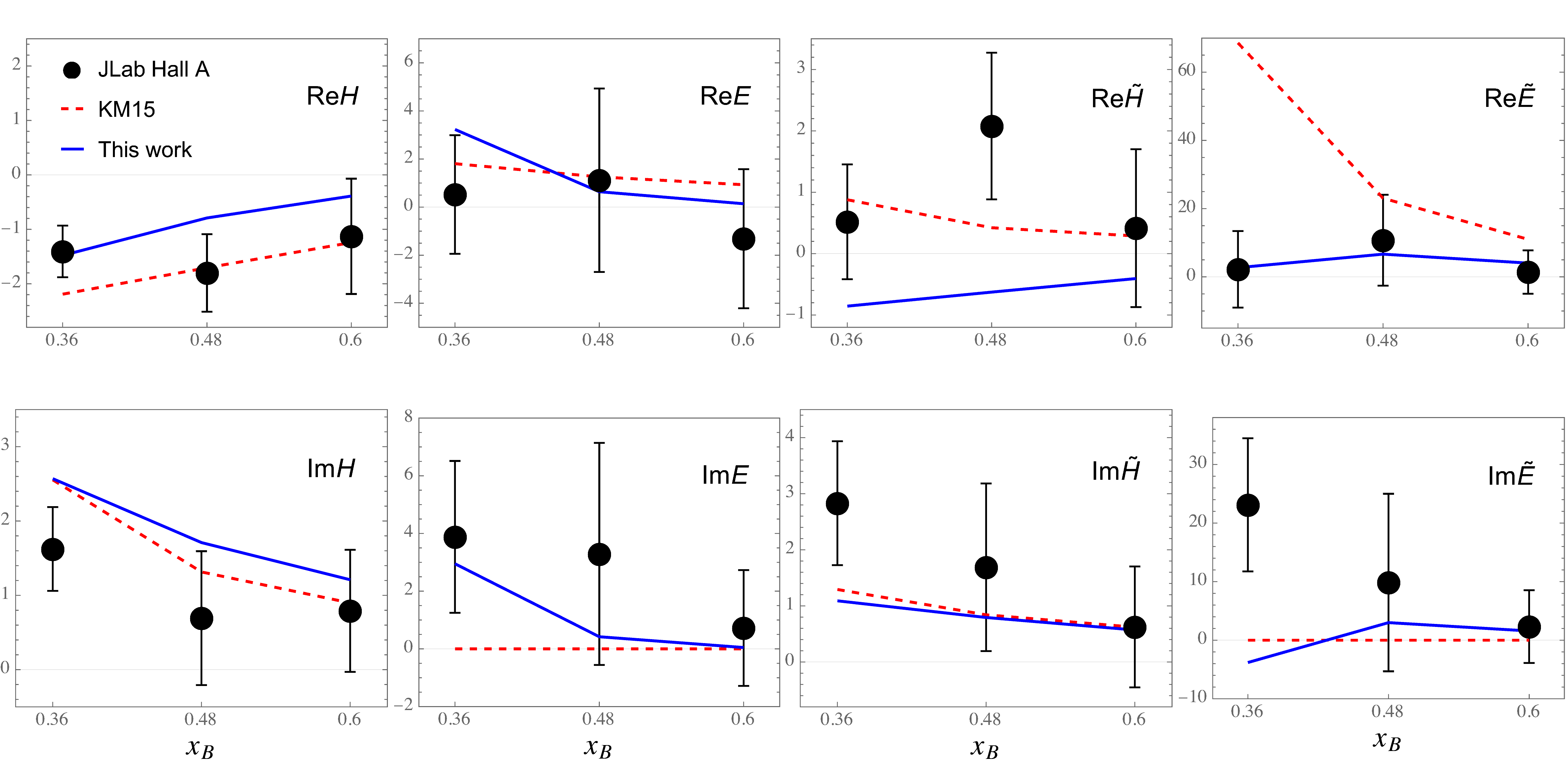
Figure 3: A comparison of the CFFs extracted in this work with the locally extracted CFFs in ref. JeffersonLabHallA:2022pnx as well as the CFFs predicted by the KM15 model Kumericki:2015lhb . The three different kinematical points with $x_{B}=0.36,0.48,0.60$ have momentum transfer $t=-0.345,-0.702,-1.050$ GeV² respectively. The CFFs in ref. JeffersonLabHallA:2022pnx are extracted from data with various different $Q^{2}$, whereas the theoretical values are calculated at the reference scale $Q^{2}=4$ GeV².

Before commenting on the comparison of the extracted CFFs, we first note that even the local extraction of CFFs suffers from the degeneracy issue. The total DVCS cross-sections are generally quadratic equations of all the 8 CFFs:

$$\text{d}\sigma^{\rm{P_{b}P_{t}}}=\text{d}\sigma^{\rm{P_{b}P_{t}}}_{\rm{DVCS}}+\text{d}\sigma^{\rm{P_{b}P_{t}}}_{\rm{INT}}+\text{d}\sigma^{\rm{P_{b}P_{t}}}_{\rm{BH}}=\sum_{i,j}A^{\rm{P_{b}P_{t}}}_{ij}\mathcal{F}^{i}\mathcal{F}^{j}+\sum_{i}B^{\rm{P_{b}P_{t}}}_{i}\mathcal{F}^{i}+C^{\rm{P_{b}P_{t}}}\ ,$$ (9)

with $\mathcal{F}_{i}=\{\text{Re}\mathcal{H},\text{Im}\mathcal{H},\text{Re}\mathcal{E},\text{Im}\mathcal{E},\text{Re}\mathcal{\widetilde{H}},\text{Im}\mathcal{\widetilde{H}},\text{Re}\mathcal{\widetilde{E}},\text{Im}\mathcal{\widetilde{E}}\}$ which are the real or imaginary parts of the CFFs corresponding to the GPDs $H$, $E$, $\widetilde{H}$ and $\widetilde{E}$. For each combination of beam polarization $P_{b}$ and target polarization $P_{t}$, the pure DVCS (DVCS), interference (INT) and Bethe-Heitler (BH) contributions are quadratic, linear, and constant in the CFFs respectively. Ideally, one would need all 8 possible combinations of $P_{b}$ and $P_{t}$ in order to disentangle the 8 CFFs, see for instance ref. Shiells:2021xqo , but there could still be degeneracy in the solutions as the nature of quadratic equations.

In this work, the degeneracy will be more severe, since only two polarization configurations, unpolarized or polarized beam with unpolarized target (UU and LU), are considered. For instance, one can show that with UU and LU cross-section, the CFF $\widetilde{\mathcal{E}}$ only shows in the quadratic terms, multiplied to either itself or $\widetilde{\mathcal{H}}$, implying that the quadratic terms are invariant under the transformation

$$\text{Re}\widetilde{\mathcal{H}}\to-\text{Re}\widetilde{\mathcal{H}}\quad,\text{Re}\widetilde{\mathcal{E}}\to-\text{Re}\widetilde{\mathcal{E}}\ ,$$ (10)

and the same for the imaginary part. This degeneracy of CFFs in the DVCS cross-sections leads to the ambiguity in the sign of the extracted $\text{Re}\widetilde{\mathcal{H}}$ and $\text{Re}\widetilde{\mathcal{E}}$ as well as the $\text{Im}\widetilde{\mathcal{H}}$ and $\text{Im}\widetilde{\mathcal{E}}$ shown on the right of figure 3, where the extracted CFFs in this work seem to take opposite sign compared to that of the local extraction. Besides this explicit example, there might be other implicit degeneracies in the extracted CFFs which could affect the reliability of such an extraction.

Although such degeneracy makes the comparison of the extracted CFFs more subtle and less intuitive, it can certainly be improved in the future with more polarization configurations taken into consideration. On the other hand, many of the CFFs extracted in this work agree well with the local extraction as shown in figure 3, adding more confidence to the extraction of those CFFs.

3.3 The extracted GPDs at non-zero skewness

Compared to the CFFs extraction discussed in the previous subsection, the extraction of GPDs will involve more model dependence. The lack of off-forward constraints except the CFFs is the main challenge in the GPD extraction, and the extracted $x$-shape of GPDs will depend on the ansatz chosen correspondingly. In addition, as the CFFs are averaged over different flavors, the extracted flavor structures could be ambiguous as well. Though suffering from these ambiguities, we still present the extracted GPDs here as an illustration of how GPDs are constrained by the inputs, with the caveat that the GPDs, especially their off-forward behaviors, are not uniquely determined at this point. These results can certainly be improved with more lattice calculation at non-zero skewness as well as more flavor-sensitive data in the future.

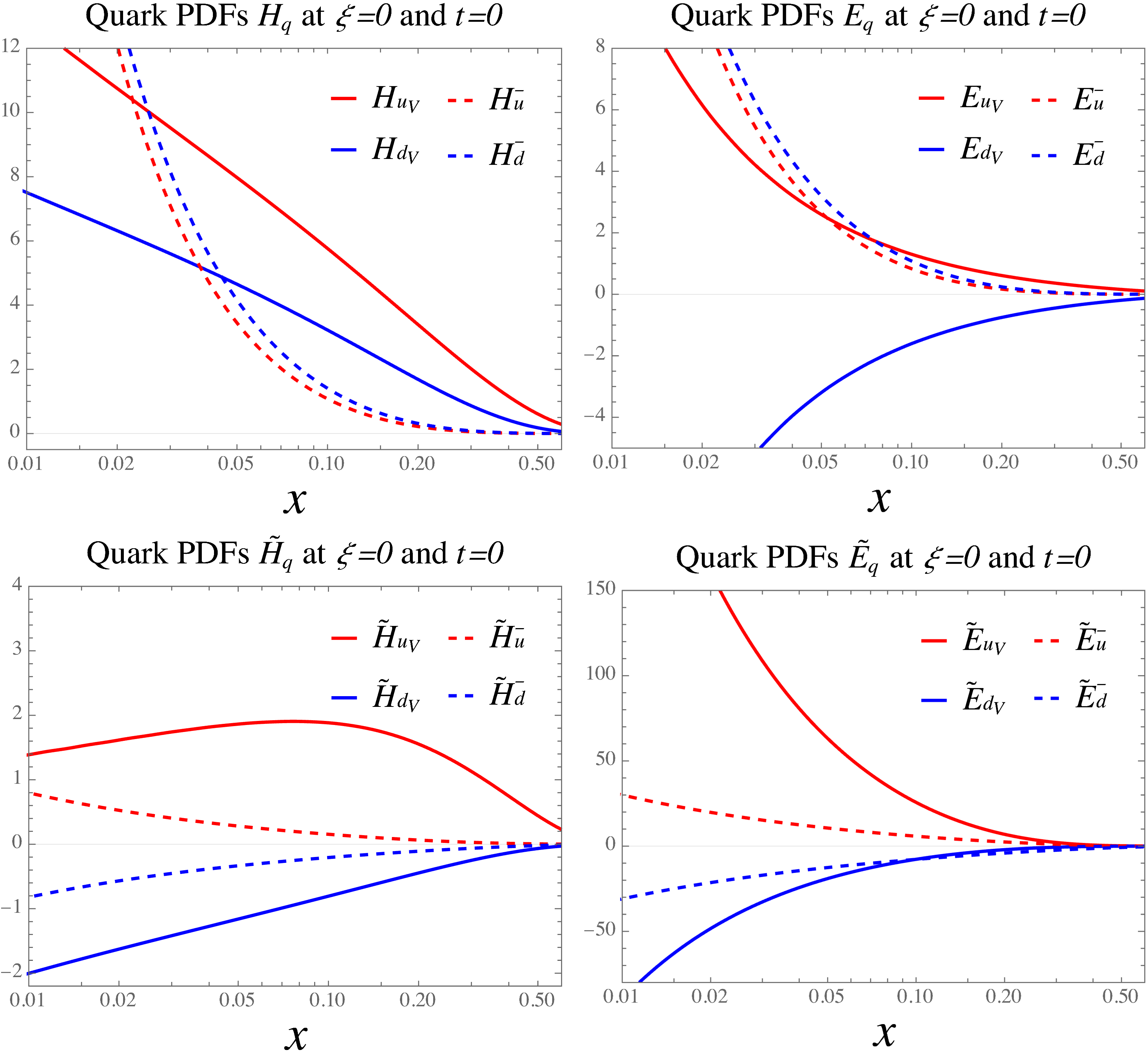
Figure 4: Plots present some examples of the extracted quark PDFs at $\xi=0$, $t=0$ and the reference scale $\mu_{0}=2$ GeV. The $H$ and $\widetilde{H}$ are obtained from the polarized and unpolarized PDFs whereas the $E$ and $\widetilde{E}$ are constrained by the form factors and lattice calculation of form factors as well as GPDs. The gluon PDFs are also implemented in this work, and they enter the scale evolutions and mix with the quark GPDs. However, since they are not as constrained by the DVCS measurements, they are not presented here.

In figure 4, we present the extracted PDFs $H$, $E$ and $\widetilde{H}$, and $\widetilde{E}$ at $\xi=0$, $t=0$, and the reference scale $\mu_{0}=2$ GeV. The two PDFs $H$ and $\widetilde{H}$ are fully parameterized and fitted to the globally extracted unpolarized and polarized PDFs in ref. Cocuzza:2022jye , and therefore they agree well with the reference values there, which are not shown in the plots though. On the other hand, due to the lack of the information, the PDFs $E$ and $\widetilde{E}$ are extracted with the empirical constraints summarized in table 1 with globally extracted FFs and lattice calculation of form factors as well as GPDs. The $\widetilde{E}$ PDFs turn out to be quite significant due to the contributions of the pion pole, according to the lattice calculated form factors of $\widetilde{E}$ Alexandrou:2021jok that we fit the $\widetilde{E}$ PDF to. As for the $E$ PDFs, the shape of the $E$ PDFs are obtained combining the lattice calculation of $E$ GPDs and other relevant form factors from both experiments and lattice results. The $u$ and $d$ quark $E$ GPDs are almost the opposite of each other, in accord with the observation that the flavor isoscalar form factors $B_{u+d}$ and gluonic gravitational form factors $B_{g}$ are consistent with zero according to the lattice results Hagler:2009ni ; Alexandrou:2021jok ; Pefkou:2021fni . We note that the valence part of the above PDFs are obtained in the semi-forward fit of the previous work Guo:2022upw as well. However, they are quantitatively slightly different from the previous results because of the different constraints used here as well as the effects of the sea quark distributions that were not considered in the previous work.

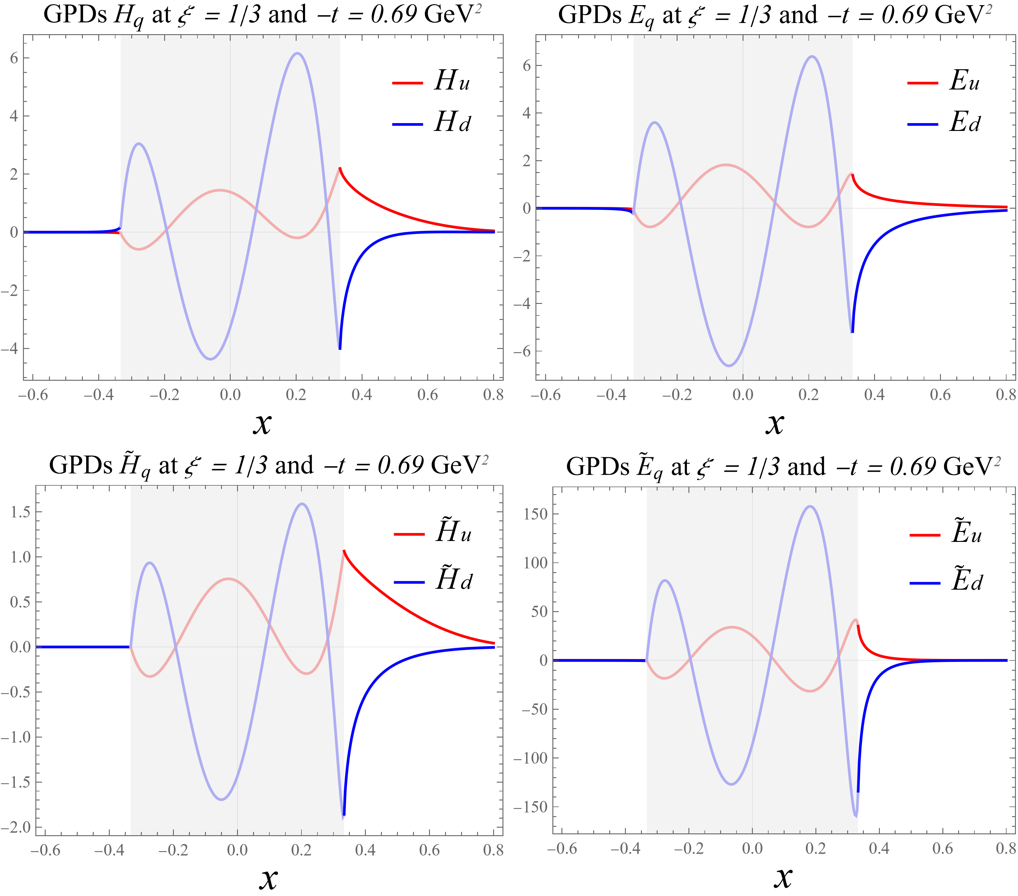
Figure 5: Plots of quark GPDs at $\xi=1/3$, $t=-0.69\text{ GeV}^{2}$ and reference scale $\mu_{0}=2$ GeV. The DA-like regions of the GPDs ($-\xi<x<\xi$) are shaded, and the curves there are plotted in lighter color for distinction. The oscillating behaviors of the GPDs in the DA-like region are the results of the conformal partial wave expansion, since the GPDs here are expanded in terms of the Gegenbauer polynomials there. We note that the shape of GPDs are determined by the model choice of the moments and the CFFs effectively constrain the GPDs at the crossover line $x=\pm\xi$ only to the leading order.

In figure 5, we present quark GPDs at $\xi=1/3$ and $t=-0.69$ GeV² and reference scale $\mu_{0}=2$ GeV. In general, the extracted GPDs oscillate in the DA-like region ($-\xi<x<\xi$) with a damping tail in the PDF-like region ($x>\xi$ or $x<-\xi$), as the result of the conformal partial wave expansion which expands the GPDs in the DA-like region in terms of Gegenbauer polynomials that oscillate. We note that due to the DA terms of GPDs, namely the $F_{q\bar{q}}$ terms in eq. (1), the behavior of GPDs in the DA-like region could look very different from here. With off-forward inputs mainly just CFFs, only the GPDs at the crossover line $x=\pm\xi$ are effectively constrained, which are then extrapolated with decaying tails to the PDF-like region, whereas the DA-like regions are not uniquely determined which we will discuss more in the next subsection.

The above extracted PDFs and GPDs are generated with the open-source codes of this program Guo:2022gumpgit which could be used to generate other observables including DVCS cross-section measurements as well, although we should note that only the central values of them are available at present. While the error propagation is a crucial part of a global analysis, the process is extremely computationally intensive. With 20 functions of three variables where each point must be calculated through a numerical contour integral, sampling them over more than 50 parameters for the statistical uncertainties would be very challenging though not as useful since the main uncertainties are still from the systematics. Therefore, we will leave the error estimation to the future works once the task will be more practical.

3.4 GPDs in the DA-like region and DA terms

In the end of this section, we discuss more about the GPDs in the DA-like region. Recall that in the previous section, we discussed that in the small $x_{B}$ expansion the DA-like region gets less relevant, and so we did not consider the DA-terms $F_{q\bar{q}}$ in the global analysis. However, the behavior of GPDs in this region is of genuine interest as well, which is less known compared to our knowledge of GPDs in the PDF-like region e.g., from PDFs. This region of GPDs is equally important and can be accessed directly from lattice calculations at non-zero skewness Alexandrou:2020zbe . We note that these constraints on GPDs in the DA-like regions were not imposed in the global analysis since only very few of them are available at present. However, in this subsection, we will discuss how the current framework under small $x_{B}$ expansion can be extended to accommodate these constraints with the extra DA-terms $F_{q\bar{q}}$ and produce smoother GPDs in the DA-like region.

In eq. (3), we showed that GPDs can be expressed as the sum of their conformal partial wave, where each term is given by a rescaled Gegenbauer polynomial Mueller:2005ed :

$$(-1)^{j}p_{j}(x,\xi)\equiv\xi^{-j-1}\frac{2^{j}\Gamma\left(\frac{5}{2}+j\right)}{\Gamma{\left(\frac{3}{2}\right)}\Gamma(j+3)}\left[1-\left(\frac{x}{\xi}\right)^{2}\right]C_{j}^{\frac{3}{2}}\left(\frac{x}{\xi}\right)\quad\text{for }|x|<\xi\ ,$$ (11)

that is non-zero only the in DA-like region. Therefore, one can always add finite terms like this to the GPDs freely without changing the GPDs in the PDF-like region. Such terms are called the DA terms in this work. Since the Wilson coefficients are antisymmetric in $x$ for the CFFs $\mathcal{H}$ and $\mathcal{E}$, adding terms with even $j$ which are symmetric in $x$ will keep both the CFFs $\mathcal{H}$ and $\mathcal{E}$ invariant, which correspond to the so-called shadow GPDs Bertone:2021yyz . On the other hand, adding terms with odd $j$ which are antisymmetric in $x$ will modify the real part of the CFFs $\mathcal{H}$ and $\mathcal{E}$ while keeping their imaginary parts the same, which are also known as the subtraction terms Kumericki:2009uq . Similar arguments apply to the $\widetilde{\mathcal{H}}$ and $\widetilde{\mathcal{E}}$ CFFs too, except that their Wilson coefficients are symmetric in $x$.

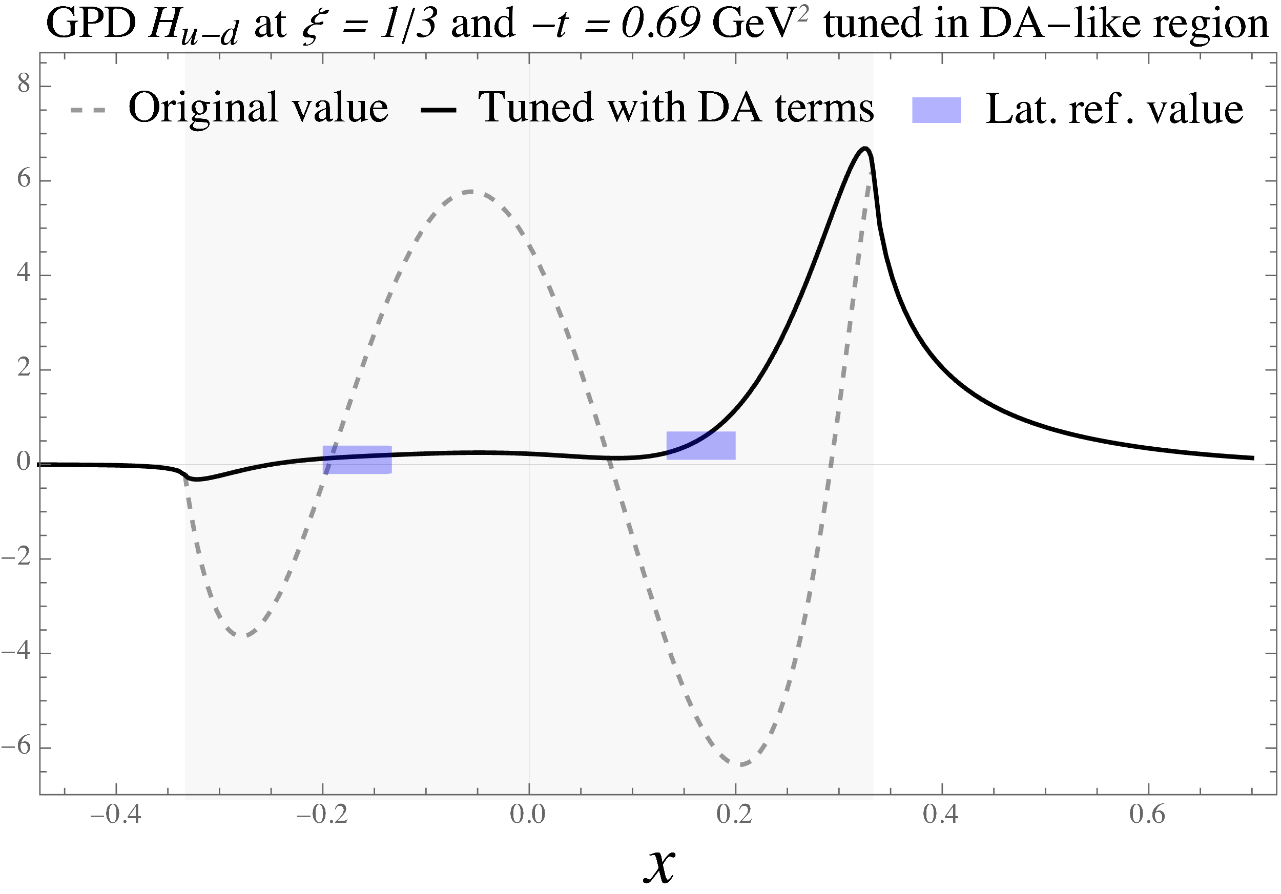
Figure 6: The isovector GPD $H_{u-d}$ tuned to fit the reference value calculated on lattice Alexandrou:2020zbe at reference scale $\mu_{0}=2$ GeV. The dashed line is the original extracted shape of GPDs. By adding extra terms in the DA-like region, we obtain the tuned GPDs as the red curve which approach the reference value shown as blue blocks.

These terms are in principle hard to extract from experiments, however, they do affect the generalized form factors and can be constrained by the FFs as well as lattice calculations. Therefore, one should parameterize these extra DA terms, at least part of them, and fit them to these constraints in order to obtain the shape of GPDs in the DA-like region. There have been lattice calculations of the GPD shape Alexandrou:2020zbe , which could be used to constrain such terms and determine the shape of GPDs in the DA-regions. However, since the results contain only the isovector $u-d$ combination of $H$ and $\widetilde{H}$ GPDs and such calculations will break down at $x=\pm\xi$, they do not pose enough constraints on the GPDs for global analysis. Therefore, we will leave the extra fitting of the DA terms to those constraints in the future work with more information in the DA-like region. In figure 6, we show an example of how GPDs can be tuned with the extra DA terms to fit to the constraints in the DA-like regions, where we take the isovector GPDs $H_{u-d}$ calculated on lattice Alexandrou:2020zbe as the reference value.

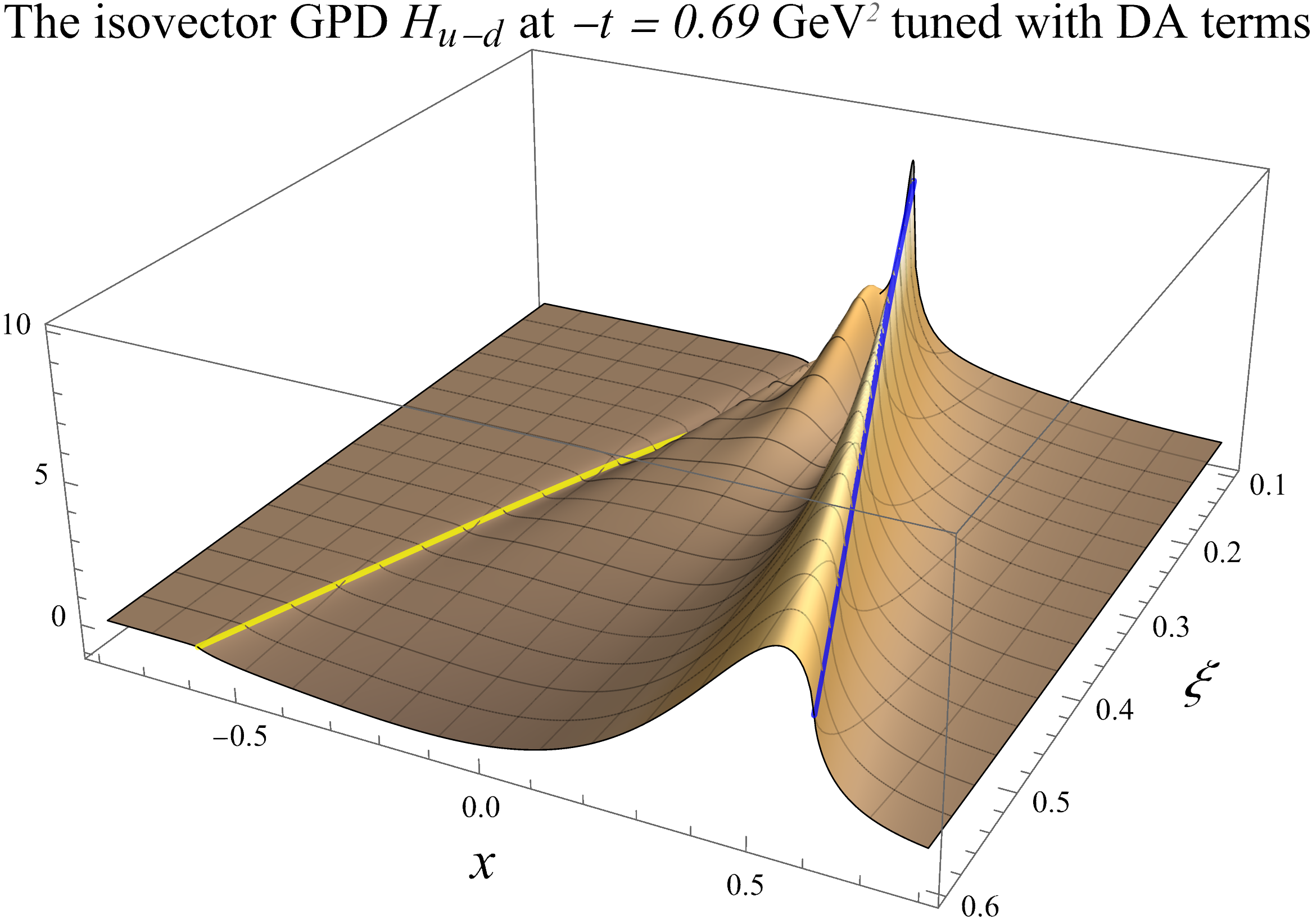
Figure 7: The isovector GPD $H_{u-d}$ on the $(x,\xi)$ plane tuned to fit the reference value calculated on lattice Alexandrou:2020zbe at $t=-0.69$ GeV² and reference scale $\mu_{0}=2$ GeV. The blue ($x=\xi$) and yellow ($x=-\xi$) curves correspond to GPDs on the two crossover lines respectively. A cut at $\xi=0.1$ is made since GPDs in the DA-like region $-\xi<x<\xi$ get singular when $\xi$ approaches $0$.

In figure 7, we also show the tuned isovector GPD $H_{u-d}$ on the $(x,\xi)$ plane at $t=-0.69$ GeV² and reference scale $\mu_{0}=2$ GeV. We again note that such results are obtained under the ansatz and empirical constraints used in this work.

4 Conclusion and outlook

We extend the previous work Guo:2022upw of the GUMP program to the non-zero skewness case and perform the global analysis of quark GPDs combing experimental measurements of DVCS, relevant lattice calculations for GPDs and PDFs and FFs from global analysis for the first time, whereas the gluon GPDs will be carried out in a separate work with other gluon-sensitive processes such as DVMP.

We argue that empirical constraints are still needed for the global analysis of GPDs, given the extremely large system of GPDs that one needs to consider and the limited knowledge of them currently. With these empirical constraints, we extract the GPDs from global analysis with the above inputs and present the globally extracted PDFs, CFFs and GPDs, with the caveat that more inputs, including more polarization configurations for the DVCS measurements and more lattice results of GPDs at non-zero skewness, are still needed to improve the reliability of such an extraction.

We also discuss the general framework to extend the current program which focuses on the small $\xi$ region of GPDs to allow the analysis of the DA-like regions of GPDs that will be more relevant at larger $\xi$. We argue that besides the quark and antiquark GPDs, the extra DA terms are crucial in describing the GPDs in the DA-like regions, which can improve the parameterization with more flexibility and without damaging the physical constraints like polynomiality conditions. We present an example how the DA terms could modify the GPDs in the DA-like region while keeping the CFFs the same, and therefore can be used to parameterize and fit the shape of GPDs in this region.

In the future works, we will consider the meson production processes in the global analysis to better constrain the gluon GPDs. In addition, we also consider adding the strange quark distributions to the analysis which might have sizable effects. Besides, we will also include the DA terms in the global analysis to fit the GPDs in the DA-like region once enough constraints on the GPDs in the DA-like region are obtained.

Appendix A GUMP parameters and their best-fit values

In this appendix we present more details of the fit, especially the best-fit parameters obtained from the global analysis. In table 3, we show all the independent parameters with their statistic uncertainties estimated by the Hessian matrix with the Minuit2 package.

Vector GPDs $H$ and $E$		Axial-vector GPDs $\widetilde{H}$ and $\widetilde{E}$
Parameter	Value (uncertainty)	Parameter	Value (uncertainty)
$N^{H}_{u_{V}}$	4.923 (89)	$N^{\widetilde{H}}_{u_{V}}$	4.833 (429)
$\alpha^{H}_{u_{V}}$	0.216 (7)	$\alpha^{\widetilde{H}}_{u_{V}}$	-0.264 (34)
$\beta^{H}_{u_{V}}$	3.229 (23)	$\beta^{\widetilde{H}}_{u_{V}}$	3.186 (122)
$\alpha^{\prime H}_{u_{V}}$	2.347 (51)	$\alpha^{\prime\widetilde{H}}_{u_{V}}$	2.182 (175)
$N^{H}_{\bar{u}}$	0.163 (8)	$N^{\widetilde{H}}_{\bar{u}}$	0.070 (33)
$\alpha^{H}_{\bar{u}}$	1.136 (10)	$\alpha^{\widetilde{H}}_{\bar{u}}$	0.538 (112)
$\beta^{H}_{\bar{u}}$	6.894 (207)	$\beta^{\widetilde{H}}_{\bar{u}}$	4.229 (1320)
$N^{H}_{d_{V}}$	3.359 (170)	$N^{\widetilde{H}}_{d_{V}}$	-0.664 (170)
$\alpha^{H}_{d_{V}}$	0.184 (18)	$\alpha^{\widetilde{H}}_{d_{V}}$	0.248 (76)
$\beta^{H}_{d_{V}}$	4.418 (77)	$\beta^{\widetilde{H}}_{d_{V}}$	3.572 (477)
$\alpha^{\prime H}_{d_{V}}$	3.482 (171)	$\alpha^{\prime\widetilde{H}}_{d_{V}}$	0.542 (103)
$N^{H}_{\bar{d}}$	0.249 (12)	$N^{\widetilde{H}}_{\bar{d}}$	-0.086 (42)
$\alpha^{H}_{\bar{d}}$	1.052 (10)	$\alpha^{\widetilde{H}}_{\bar{d}}$	0.495 (137)
$\beta^{H}_{\bar{d}}$	6.554 (216)	$\beta^{\widetilde{H}}_{\bar{d}}$	2.554 (897)
$N^{H}_{g}$	2.864 (108)	$N^{\widetilde{H}}_{g}$	0.243 (304)
$\alpha^{H}_{g}$	1.052 (8)	$\alpha^{\widetilde{H}}_{g}$	0.631 (330)
$\beta^{H}_{g}$	7.413 (165)	$\beta^{\widetilde{H}}_{g}$	2.717 (2865)
$N^{E}_{u_{V}}$	0.181 (38)	$N^{\widetilde{E}}_{u_{V}}$	7.993 (3480)
$\alpha^{E}_{u_{V}}$	0.907 (17)	$\alpha^{\widetilde{E}}_{u_{V}}$	0.800 (116)
$\beta^{E}_{u_{V}}$	1.102 (245)	$\beta^{\widetilde{E}}_{u_{V}}$	6.415 (1577)
$\alpha^{\prime E}_{u_{V}}$	0.461 (86)	$\alpha^{\prime\widetilde{E}}_{u_{V}}$	2.076 (933)
$N^{E}_{d_{V}}$	-0.223 (47)	$N^{\widetilde{E}}_{d_{V}}$	-2.407 (1239)
$R^{E}_{\rm{sea}}$	0.768 (169)	$R^{\widetilde{E}}_{\rm{sea}}$	38 (8)
$R^{H}_{u,2}$	0.229 (0.032)	$R^{\widetilde{H}}_{u,2}$	0.246 (81)
$R^{H}_{d,2}$	-2.639 (202)	$R^{\widetilde{H}}_{d,2}$	1.656 (375)
$R^{E}_{u,2}$	0.799 (285)	$R^{\widetilde{E}}_{u,2}$	2.684 (171)
$R^{E}_{d,2}$	3.404 (1157)	$R^{\widetilde{E}}_{d,2}$	38 (2)
$b^{H}_{\rm{sea}}$	3.448 (133)	$b^{\widetilde{H}}_{\rm{sea}}$	9.852 (1330)

Table 3: A summary of the obtained independent GUMP parameters.

We note that the $N,\alpha,\beta,\alpha^{\prime},b$ are the parameters in the moments of GPDs according to eq. (6) where $\alpha(t)\equiv\alpha+\alpha^{\prime}t$ corresponds to the linear Regge trajectory and $\beta(t)=\exp(bt)$ corresponds to the extra exponential term. Each of these parameters have a superscript representing its GPD species ($H$, $E$, $\widetilde{H}$ or $\widetilde{E}$) and a subscript representing its flavor ($u_{V}$, $\bar{u}$, $d_{V}$, $\bar{d}$ or $g$). The $R^{E}_{\rm{sea}}$ and $R^{\widetilde{E}}_{\rm{sea}}$ are the ratio of the $E(\widetilde{E})$ GPDs to the $H(\widetilde{H})$ GPDs for the sea quarks and gluons. Besides them, there are also parameters like $R^{H}_{u,2}$ that are the ratio of the $\xi^{2}$ terms to the forward terms as defined in eq. (7) for GPDs with different species and flavors. We again note that more details of them and the GUMP program that generate the GUMP GPDs, CFFs and cross-sections are available online Guo:2022gumpgit .

References

- (1) D. Müller, D. Robaschik, B. Geyer, F.M. Dittes and J. Hořejši, Wave functions, evolution equations and evolution kernels from light ray operators of QCD, Fortsch. Phys. 42 (1994) 101 [hep-ph/9812448].
- (2) X.-D. Ji, Gauge-Invariant Decomposition of Nucleon Spin, Phys. Rev. Lett. 78 (1997) 610 [hep-ph/9603249].
- (3) X.-D. Ji, Off forward parton distributions, J. Phys. G 24 (1998) 1181 [hep-ph/9807358].
- (4) X.-D. Ji, A QCD analysis of the mass structure of the nucleon, Phys. Rev. Lett. 74 (1995) 1071 [hep-ph/9410274].
- (5) M.V. Polyakov, Generalized parton distributions and strong forces inside nucleons and nuclei, Phys. Lett. B 555 (2003) 57 [hep-ph/0210165].
- (6) X.-D. Ji, Deeply virtual Compton scattering, Phys. Rev. D 55 (1997) 7114 [hep-ph/9609381].
- (7) A.V. Radyushkin, Asymmetric gluon distributions and hard diffractive electroproduction, Phys. Lett. B 385 (1996) 333 [hep-ph/9605431].
- (8) J.C. Collins, L. Frankfurt and M. Strikman, Factorization for hard exclusive electroproduction of mesons in QCD, Phys. Rev. D 56 (1997) 2982 [hep-ph/9611433].
- (9) CLAS collaboration, Exploring the Structure of the Bound Proton with Deeply Virtual Compton Scattering, Phys. Rev. Lett. 123 (2019) 032502 [1812.07628].
- (10) CLAS collaboration, Beam charge asymmetries for deeply virtual Compton scattering off the proton, Eur. Phys. J. A 57 (2021) 186 [2103.12651].
- (11) Jefferson Lab Hall A collaboration, Deeply Virtual Compton Scattering at 11GeV in Jefferson Lab Hall A, PoS Hadron2017 (2018) 170.
- (12) Jefferson Lab Hall A collaboration, Deeply Virtual Compton Scattering Cross Section at High Bjorken xB, Phys. Rev. Lett. 128 (2022) 252002 [2201.03714].
- (13) A. Accardi et al., Electron Ion Collider: The Next QCD Frontier: Understanding the glue that binds us all, Eur. Phys. J. A 52 (2016) 268 [1212.1701].
- (14) R. Abdul Khalek et al., Science Requirements and Detector Concepts for the Electron-Ion Collider: EIC Yellow Report, 2103.05419.
- (15) X. Ji, Parton Physics on a Euclidean Lattice, Phys. Rev. Lett. 110 (2013) 262002 [1305.1539].
- (16) X. Ji, Y.-S. Liu, Y. Liu, J.-H. Zhang and Y. Zhao, Large-momentum effective theory, Rev. Mod. Phys. 93 (2021) 035005 [2004.03543].
- (17) C. Alexandrou, K. Cichy, M. Constantinou, K. Hadjiyiannakou, K. Jansen, A. Scapellato et al., Unpolarized and helicity generalized parton distributions of the proton within lattice QCD, Phys. Rev. Lett. 125 (2020) 262001 [2008.10573].
- (18) H.-W. Lin, Nucleon helicity generalized parton distribution at physical pion mass from lattice QCD, Phys. Lett. B 824 (2022) 136821 [2112.07519].
- (19) T.-J. Hou et al., New CTEQ global analysis of quantum chromodynamics with high-precision data from the LHC, Phys. Rev. D 103 (2021) 014013 [1912.10053].
- (20) NNPDF collaboration, The path to proton structure at 1% accuracy, Eur. Phys. J. C 82 (2022) 428 [2109.02653].
- (21) J.J. Ethier, N. Sato and W. Melnitchouk, First simultaneous extraction of spin-dependent parton distributions and fragmentation functions from a global QCD analysis, Phys. Rev. Lett. 119 (2017) 132001 [1705.05889].
- (22) Z. Ye, J. Arrington, R.J. Hill and G. Lee, Proton and Neutron Electromagnetic Form Factors and Uncertainties, Phys. Lett. B 777 (2018) 8 [1707.09063].
- (23) C. Alexandrou, S. Bacchio, M. Constantinou, J. Finkenrath, K. Hadjiyiannakou, K. Jansen et al., Nucleon form factors from =2+1+1 twisted mass QCD at the physical point, PoS LATTICE2021 (2022) 250 [2112.06750].
- (24) N. Hasan, J. Green, S. Meinel, M. Engelhardt, S. Krieg, J. Negele et al., Computing the nucleon charge and axial radii directly at in lattice QCD, Phys. Rev. D 97 (2018) 034504 [1711.11385].
- (25) E. Shintani, K.-I. Ishikawa, Y. Kuramashi, S. Sasaki and T. Yamazaki, Nucleon form factors and root-mean-square radii on a (10.8 fm)4 lattice at the physical point, Phys. Rev. D 99 (2019) 014510 [1811.07292].
- (26) PNDME collaboration, Updates on Nucleon Form Factors from Clover-on-HISQ Lattice Formulation, PoS LATTICE2018 (2018) 123 [1901.00060].
- (27) M.V. Polyakov and A.G. Shuvaev, On’dual’ parametrizations of generalized parton distributions, hep-ph/0207153.
- (28) M. Guidal, M.V. Polyakov, A.V. Radyushkin and M. Vanderhaeghen, Nucleon form-factors from generalized parton distributions, Phys. Rev. D 72 (2005) 054013 [hep-ph/0410251].
- (29) S.V. Goloskokov and P. Kroll, Vector meson electroproduction at small Bjorken-x and generalized parton distributions, Eur. Phys. J. C 42 (2005) 281 [hep-ph/0501242].
- (30) D. Mueller and A. Schafer, Complex conformal spin partial wave expansion of generalized parton distributions and distribution amplitudes, Nucl. Phys. B 739 (2006) 1 [hep-ph/0509204].
- (31) K. Kumerički and D. Mueller, Deeply virtual Compton scattering at small and the access to the GPD H, Nucl. Phys. B 841 (2010) 1 [0904.0458].
- (32) G.R. Goldstein, J.O. Hernandez and S. Liuti, Flexible Parametrization of Generalized Parton Distributions from Deeply Virtual Compton Scattering Observables, Phys. Rev. D 84 (2011) 034007 [1012.3776].
- (33) J.O. Gonzalez-Hernandez, S. Liuti, G.R. Goldstein and K. Kathuria, Interpretation of the Flavor Dependence of Nucleon Form Factors in a Generalized Parton Distribution Model, Phys. Rev. C 88 (2013) 065206 [1206.1876].
- (34) B. Kriesten, P. Velie, E. Yeats, F.Y. Lopez and S. Liuti, Parametrization of Quark and Gluon Generalized Parton Distributions in a Dynamical Framework, 2101.01826.
- (35) H. Hashamipour, M. Goharipour, K. Azizi and S.V. Goloskokov, Determination of the generalized parton distributions through the analysis of the world electron scattering data considering two-photon exchange corrections, Phys. Rev. D 105 (2022) 054002 [2111.02030].
- (36) Y. Guo, X. Ji and K. Shiells, Generalized parton distributions through universal moment parameterization: zero skewness case, JHEP 09 (2022) 215 [2207.05768].
- (37) H1 collaboration, Deeply Virtual Compton Scattering and its Beam Charge Asymmetry in e+- Collisions at HERA, Phys. Lett. B 681 (2009) 391 [0907.5289].
- (38) M. Čuić, K. Kumerički and A. Schäfer, Separation of Quark Flavors Using Deeply Virtual Compton Scattering Data, Phys. Rev. Lett. 125 (2020) 232005 [2007.00029].
- (39) K. Kumericki, D. Mueller and K. Passek-Kumericki, Towards a fitting procedure for deeply virtual Compton scattering at next-to-leading order and beyond, Nucl. Phys. B 794 (2008) 244 [hep-ph/0703179].
- (40) M.V. Polyakov and C. Weiss, Skewed and double distributions in pion and nucleon, Phys. Rev. D 60 (1999) 114017 [hep-ph/9902451].
- (41) K. Goeke, M.V. Polyakov and M. Vanderhaeghen, Hard exclusive reactions and the structure of hadrons, Prog. Part. Nucl. Phys. 47 (2001) 401 [hep-ph/0106012].
- (42) M. Diehl, Generalized parton distributions, Phys. Rept. 388 (2003) 41 [hep-ph/0307382].
- (43) D. Müller, M.V. Polyakov and K.M. Semenov-Tian-Shansky, Dual parametrization of generalized parton distributions in two equivalent representations, JHEP 03 (2015) 052 [1412.4165].
- (44) H1 collaboration, Measurement of deeply virtual Compton scattering and its t-dependence at HERA, Phys. Lett. B 659 (2008) 796 [0709.4114].
- (45) H1 collaboration, Elastic J/psi production at HERA, Eur. Phys. J. C 46 (2006) 585 [hep-ex/0510016].
- (46) V. Bertone, H. Dutrieux, C. Mezrag, H. Moutarde and P. Sznajder, Deconvolution problem of deeply virtual Compton scattering, Phys. Rev. D 103 (2021) 114019 [2104.03836].
- (47) D. Müller, T. Lautenschlager, K. Passek-Kumericki and A. Schaefer, Towards a fitting procedure to deeply virtual meson production - the next-to-leading order case, Nucl. Phys. B 884 (2014) 438 [1310.5394].
- (48) D. Mueller, Generalized Parton Distributions – visions, basics, and realities –, Few Body Syst. 55 (2014) 317 [1405.2817].
- (49) Jefferson Lab Angular Momentum (JAM) collaboration, Polarized antimatter in the proton from a global QCD analysis, Phys. Rev. D 106 (2022) L031502 [2202.03372].
- (50) Jefferson Lab Angular Momentum (JAM) collaboration, How well do we know the gluon polarization in the proton?, Phys. Rev. D 105 (2022) 074022 [2201.02075].
- (51) M. Constantinou et al., Parton distributions and lattice-QCD calculations: Toward 3D structure, Prog. Part. Nucl. Phys. 121 (2021) 103908 [2006.08636].
- (52) E.R. Berger, M. Diehl and B. Pire, Time - like Compton scattering: Exclusive photoproduction of lepton pairs, Eur. Phys. J. C 23 (2002) 675 [hep-ph/0110062].
- (53) CLAS collaboration, First Measurement of Timelike Compton Scattering, Phys. Rev. Lett. 127 (2021) 262501 [2108.11746].
- (54) ZEUS collaboration, Exclusive electroproduction of phi mesons at HERA, Nucl. Phys. B 718 (2005) 3 [hep-ex/0504010].
- (55) H. Dembinski and P.O. et al., scikit-hep/iminuit, .
- (56) F. James and M. Roos, Minuit: A System for Function Minimization and Analysis of the Parameter Errors and Correlations, Comput. Phys. Commun. 10 (1975) 343.
- (57) Y. Guo, X. Ji and K. Shiells, Higher-order kinematical effects in deeply virtual Compton scattering, JHEP 12 (2021) 103 [2109.10373].
- (58) Y. Guo, X. Ji, B. Kriesten and K. Shiells, Twist-three cross-sections in deeply virtual Compton scattering, JHEP 06 (2022) 096 [2202.11114].
- (59) V.M. Braun, A.N. Manashov, D. Müller and B.M. Pirnay, Deeply Virtual Compton Scattering to the twist-four accuracy: Impact of finite- and target mass corrections, Phys. Rev. D 89 (2014) 074022 [1401.7621].
- (60) K. Kumerički and D. Müller, Description and interpretation of DVCS measurements, EPJ Web Conf. 112 (2016) 01012 [1512.09014].
- (61) K. Shiells, Y. Guo and X. Ji, On extraction of twist-two Compton form factors from DVCS observables through harmonic analysis, JHEP 08 (2022) 048 [2112.15144].
- (62) P. Hagler, Hadron structure from lattice quantum chromodynamics, Phys. Rept. 490 (2010) 49 [0912.5483].
- (63) D.A. Pefkou, D.C. Hackett and P.E. Shanahan, Gluon gravitational structure of hadrons of different spin, Phys. Rev. D 105 (2022) 054509 [2107.10368].
- (64) Y. Guo et al., “GUMP GPD Global Analysis.” https://github.com/yuxunguo/GUMP-Global-GPDs, 2022.
- (65) K. Kumerički, “Gepard: Tool for studying the 3D quark and gluon distributions in the nucleon.” https://gepard.phy.hr.