HST viewing of spectacular star-forming trails behind ESO 137/̄001

Abstract

We present the results from the HST WFC3 and ACS data on an archetypal galaxy undergoing ram pressure stripping (RPS), ESO 137/̄001, in the nearby cluster Abell 3627. ESO 137/̄001 is known to host a prominent stripped tail detected in many bands from X-rays, H$\alpha$ to CO. The HST data reveal significant features indicative of RPS such as asymmetric dust distribution and surface brightness as well as many blue young star complexes in the tail. We study the correlation between the blue young star complexes from HST, H ii regions from H$\alpha$ (MUSE) and dense molecular clouds from CO (ALMA). The correlation between the HST blue star clusters and the H ii regions is very good, while their correlation with the dense CO clumps are typically not good, presumably due in part to evolutionary effects. In comparison to the Starburst99+Cloudy model, many blue regions are found to be young ($<$ 10 Myr) and the total star formation (SF)rate in the tail is 0.3 - 0.6 M_☉/yr for sources measured with ages less than 100 Myr, about 40% of the SF rate in the galaxy. We trace SF over at least 100 Myr and give a full picture of the recent SF history in the tail. We also demonstrate the importance of including nebular emissions and a nebular to stellar extinction correction factor when comparing the model to the broadband data. Our work on ESO 137/̄001 demonstrates the importance of HST data for constraining the SF history in stripped tails.

1 Introduction

It has been long known that the environments where galaxies reside affect their properties and evolution (e.g., Dressler, 1980; Boselli et al., 2022). Galaxies can be shaped by gravitational processes, e.g., mergers and tidal stripping. Another important process that shapes galaxies, especially in galaxy clusters and groups, is ram pressure stripping (Gunn & Gott, 1972; Boselli et al., 2022). Ram pressure stripping (RPS) on galaxies comes from the drag force from the surrounding medium that is proportional to its density and the square of the galaxy velocity. RPS can impact galaxy evolution by first compressing the disk’s interstellar medium (ISM) triggering an initial star burst (e.g., Bekki & Couch, 2003). Once RPS sweeps through the galaxy, the cold ISM will be removed, eventually quenching star formation in the galaxy (e.g. Quilis et al., 2000). RPS can have a significant impact on the properties of galaxies, e.g., disk truncation, formation of flocculent arms, transformation of dwarf galaxies and nuclear activity (see recent review by Boselli et al. 2022). In recent years, evidence of RPS has been found in many clusters across different bands on different gas tracers from H i, H$\alpha$, warm H₂, X-rays to CO (see the recent review by Boselli et al. 2022). It has been gradually established that the cold ISM, once stripped from galaxies, will mix with the surrounding hot intracluster medium (ICM). During the process, a fraction of the stripped ISM can cool to form stars in the tails, while the bulk will eventually be evaporated (e.g., Sun et al., 2022). Nevertheless, many outstanding questions remain, e.g., the impact of RPS on galaxy properties, the star formation (SF) efficiency in tails, roles of magnetic field and turbulence, and the spatial and kinematic connection for gas of different phases. To address these questions, a multi-wavelength approach is required. Among all the multi-wavelength data, optical/UV broad-band data with HST present the sharpest view of SF in the stripped tails and allow detailed constraints on the “sink term” of the multi-phase stripped tails.

This work presents this type of study with the Hubble Space Telescope (HST) data, on the archetypal RPS galaxy, ESO 137/̄001, also the one with the brightest diffuse H$\alpha$ tail and the richest amount of multi-wavelength supporting data (Sun et al., 2007; Sun et al., 2010; Sivanandam et al., 2010; Fumagalli et al., 2014; Jáchym et al., 2014; Fossati et al., 2016; Jáchym et al., 2019; Sun et al., 2022). It is also the only RPS galaxy in the JWST GTO program with 14.5 hours of MIRI observations (program 1178). Here we study the impact of RPS on the galaxy. We intend to quantify the star formation rate (SFR) in the tail and compare the HST results with those from H$\alpha$ observations (as similarly done in e.g., Cramer et al. 2019 and Poggianti et al. 2019). The SFR history in the tail is also examined, as well as connection between young star clusters/complexes, H ii, regions and CO clouds.

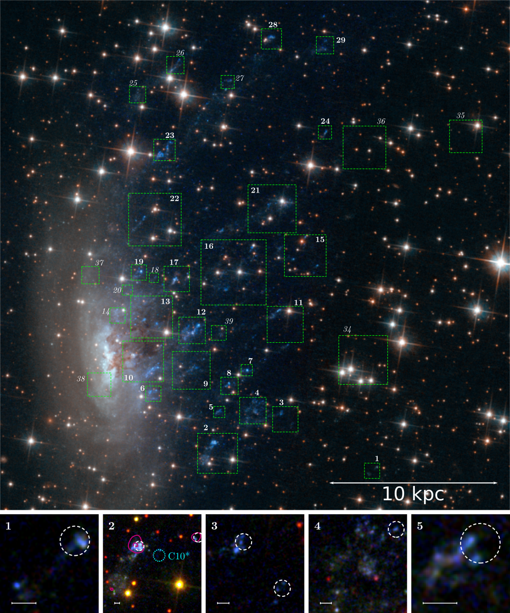
Figure 1: The RGB image (blue: F275W; green: F475W; red: F814W) of ESO 137/̄001 with zoom-ins on 40 regions (Large Image Credit: STScI; zoom-ins are from this work). We include the following zoom-in regions: H ii regions defined in Section 4.1 shown by the white, dashed circles with a radius of 0$\aas@@fstack{\prime\prime}$40, X-ray point sources from Sun et al. (2010) shown by the cyan, dotted circles with a radius of 0$\aas@@fstack{\prime\prime}$50, bright CO sources from Jáchym et al. (2019) shown by the magenta, solid contours (contour levels of 0.03, 0.06 and 0.12 Jy km/s per beam), and blue star clusters defined from this work. The blue star clusters shown were selected with these criteria: F275W-F475W < 2, F475W-F814W < 1 and F475W < 25.6. Some isolated blue sources are not included in zoom-ins but they are all studied in this work. The arrow on each cutout represents 0.25 kpc. The bold numbers emphasize regions that align with an H ii source, and italicized numbers emphasize regions that do not. Regions 30, 31, 32, 33, and 40 lie outside the large STScI image and are shown for reference on Fig. 7. Region 40 is not covered by F275W so the blue source associated with the H ii region appears green. The correlation of H ii, blue HST star clusters, CO clumps and X-ray sources is discussed in Section 4.

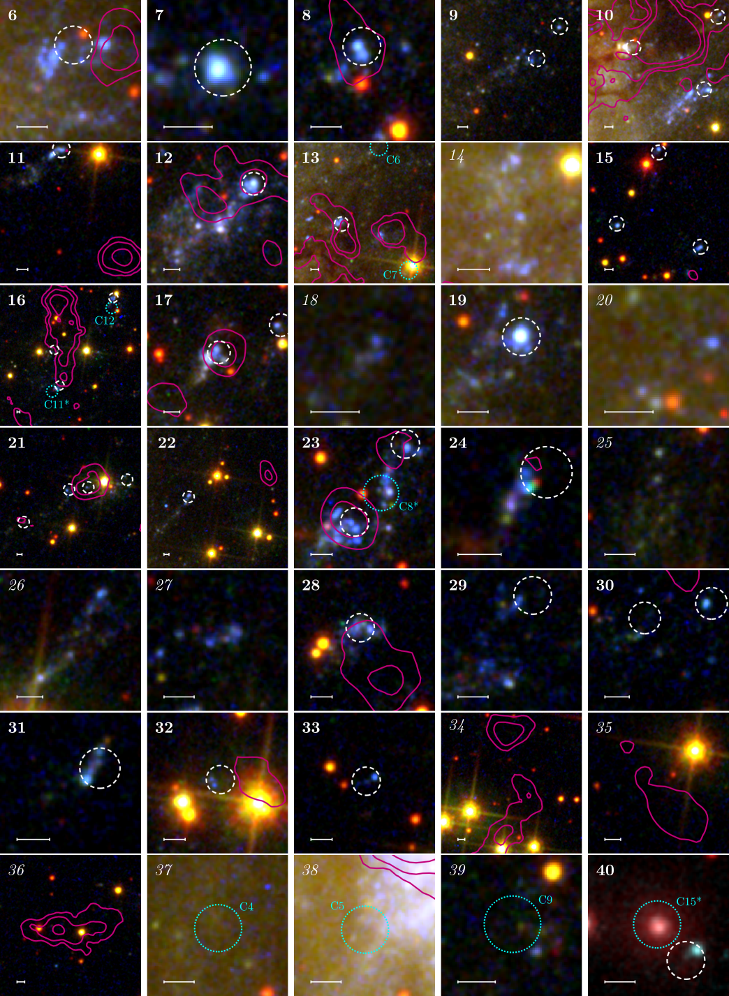
Figure 2: continued

More zoom-ins.

ESO 137/̄001 (see Fig. 1), a spiral galaxy near the center of the closest rich cluster, the Norma cluster (Abell 3627), was first discovered as a galaxy undergoing RPS by Sun et al. (2006, hereafter S06) with the Chandra and XMM X-ray data that reveal a 70 kpc long, narrow X-ray tail. Sun et al. (2007, hereafter S07) took the narrow-band imaging data with the Southern Observatory for Astrophysical Research (SOAR) telescope to discover a 40 kpc H$\alpha$ tail that aligned with the X-ray tail. More than 30 H ii regions were also revealed, unambiguously confirming SF in the stripped ISM. Sun et al. (2010, hereafter S10) further studied ESO 137/̄001 with deeper Chandra observations and Gemini spectroscopic observations. The deep Chandra data surprisingly revealed that the X-ray tail, now detected to at least 80 kpc from the galaxy, is bifurcated with a secondary branch on the south of the primary X-ray tail. Re-examination of the S07 H$\alpha$ data also shows H$\alpha$ enhancement at several positions of the secondary tail. S10 also presented the Gemini spectra of over 33 H ii regions and revealed the imprint of the galactic rotation pattern in the tail.

Sivanandam et al. (2010) presented Spitzer data on ESO 137/̄001 that reveals a 20 kpc warm (130-160 K) H₂ tail which is co-aligned with the X-ray and the H$\alpha$ tail (note that the extent of the H₂ tail is limited by the field of view of the IRS instrument). The large H₂ line to IR continuum luminosity ratio suggests that SF is not the main excitation source in the tail. Jáchym et al. (2014) used APEX telescope to observe ESO 137/̄001 and its tail at four positions. Strong CO(2-1) emission is detected at each position, including the middle of the primary tail that is 40 kpc from the galaxy, indicating abundant cold molecular gas in the tail. On the other hand, the SF efficiency in the tail appears to be low. Jáchym et al. (2019) further observed ESO 137/̄001 and its tail with a mosiac from the Atacama Large Millimeter Array (ALMA) to obtain a high-resolution view of the cold molecular gas. The resulting map reveals a rich amount of molecular cloud structure in the tail, ranging from compact clumps associated with H ii regions, large clumps not closely associated with any H ii regions, to long filaments away from any SF regions.

Spatially resolved studies of warm, ionized gas have been revolutionized with the Multi Unit Spectroscopic Explorer (MUSE) on VLT. As the first science paper with MUSE, Fumagalli et al. (2014) presented results from the MUSE observations on ESO 137/̄001 and the front half of the primary tail. The work demonstrates the great potential of MUSE on studies of diffuse warm, ionized gas as often seen in stripped tails. The early MUSE velocity and velocity dispersion maps suggest that turbulence begins to be dominant at $>$ 6.5 Myr after stripping. Fossati et al. (2016, hereafter F16), with the same MUSE data that Fumagalli et al. (2014) used, presented a detailed study of line diagnostics in ESO 137/̄001’s tail. Their results also called for better modeling of ionization mechanisms in stripped tails. Sun et al. (2022) presented a new MUSE mosaic to cover the full extent of ESO 137/̄001’s tail, revealing very good correlation with the X-ray emission. This new set of MUSE data provides a great amount of data for detailed studies of kinematics and line diagnostics (Luo et al., 2022).

As discussed above, ESO 137/̄001 has become the RPS galaxy with the richest amount of supporting data and multi-wavelength analysis. In this context, a detailed study with the HST data adds important information on this multi-wavelength campaign, which is the focus of this paper. Table 1 summarizes the properties of ESO 137/̄001. As in S10, we adopt a luminosity distance of 69.6 Mpc for Abell 3627 and $1\arcsec{}=0.327$ kpc. The rest of the paper proceeds as follows: Section 2 details the HST observations and the data reduction. Section 3 focuses on the properties of ESO 137/̄001. Section 4 presents the studies of the young star complexes discovered in the tail of ESO 137/̄001. Section 5 is the discussion and we present our conclusions in Section 6.

Table 1: Properties of ESO 137-001

Heliocentric velocity (km/s)a	4647 (-224)
Offset (kpc)b	180
Position Angle	$\sim$ 9∘
Inclination	$\sim$ 66∘
$W1$ (Vega mag)c	12.31
$L_{\rm W1}$ ($10^{9}L_{\odot}$)c	0.489
$W1-W4$ (Vega mag) c	6.99
$m_{\rm F160W}$ (AB mag)d	13.16
Half light semi-major axis (kpc)d	4.91
M⋆ ($10^{9}M_{\odot})^{\mathrm{e}}$	5-8
$M_{\rm mol}$ ($10^{9}M_{\odot}$)f	$\sim$ 1.1
LFIR ($10^{9}L_{\odot})$g	5.2
SFR (M⊙/yr) (Galaxy)h	1.2
M⋆ ($10^{6}M_{\odot})$ (Tail)	2.5 - 3.0
SFR (M⊙/yr) (Tail)	0.4 - 0.65
Tail length (kpc)i	80 - 87 (X-ray/H$\alpha$)

Note:
^(a) The heliocentric velocity of the galaxy from our study on the stellar spectrum around the nucleus (Luo et al. 2022). The velocity value in parentheses is the radial velocity relative to that of Abell 3627 (Woudt et al., 2004).
^(b) The projected offset of the galaxy from the X-ray center of A3627
^(c) The WISE 3.4 $\mu$m magnitude, luminosity and the WISE 3.4 $\mu$m - 22 $\mu$m color. The Galactic extinction was corrected with the relation from Indebetouw et al. (2005).
^(d) The total magnitude and the half light semi-major axis at the F160W band. The axis ratio is 2.27 and the positional angle is $9.0^{\circ}$ east of the North.
^(e) The total stellar mass estimated from S10.
^(f) The total amount of the molecular gas detected in the galaxy from Jáchym et al. (2014).
^(g) The total FIR luminosity from the Herschel data (see Section 5.1)
^(h) The average value from the first estimate (0.97) based on the Galex NUV flux density and the total FIR luminosity from Herschel with the relation from Hao et al. (2011), and the second estimate (1.4) based on the WISE 22 $\mu$m flux density with the relation from Lee et al. (2013). The Kroupa initial mass function (IMF)is assumed.
⁽ⁱ⁾ The tail length for ESO 137-001 from S10.

2 HST Observations and Data Analysis

The data for this work were collected using the Wide Field Camera 3 (WFC3) and Advanced Camera System (ACS) on HST, from proposals 11683 and 12372 (PI: Ming Sun). Details of the observations are summarized in Table 2. All observations focus on the tail of ESO 137/̄001 described in Sun et al. (2006); Sun et al. (2007). The F275W data are especially sensitive to recent star formation in the last several $10^{7}$ years and the F275W - F475W color measures the strength of the 4000 Å break. The data from F475W and F814W add a broad spectrum of light to identify dim, diffuse features, while the F160W data present the view of the galaxy least affected by the dust extinction. Together, these four filters can be used to constrain the stellar age of star clusters found in the galaxy and the tail. The HST WFC3 UVIS Channel has a pixel scale of 0$\aas@@fstack{\prime\prime}$04 per pixel (13 pc/pix) with a point spread function (PSF) full width at half maximum (FWHM) of 0$\aas@@fstack{\prime\prime}$067 to 0$\aas@@fstack{\prime\prime}$089 (22 pc to 29 pc; Dressel, 2022). The HST WFC3 IR Channel has a pixel scale of 0$\aas@@fstack{\prime\prime}$13 per pixel (43 pc/pix) with a PSF FWHM of 0$\aas@@fstack{\prime\prime}$124 to 0$\aas@@fstack{\prime\prime}$156 (41 pc to 51 pc; Dressel, 2022). The HST ACS Wide Field Channel has a pixel scale of 0$\aas@@fstack{\prime\prime}$05 per pixel (16 pc/pix) with a recoverable reconstructed FWHM of 0$\aas@@fstack{\prime\prime}$100 to 0$\aas@@fstack{\prime\prime}$140 (33 pc to 46 pc) after dithering (Ryon, 2022).

Table 2: HST Observations (PI: Sun)

Filter	Instrument	Mode	Dithera	Date	Exp (sec)	Mean $\lambda$ / FWHM (Å)
F275W	WFC3/UVIS	ACCUM	3 (2.4′′)	02/08/2009	$3\times 978.0$	2719/418
F475W	ACS/WFC	ACCUM	2 (3.01′′)	02/08/2009	$2\times 871.0$	4802/1437
F814W	ACS/WFC	ACCUM	2 (3.01′′)	02/08/2009	$2\times 339.0$	8129/1856
F160W	WFC3/IR	MULTIACCUM	3 (0.605′′)	17/07/2011	$3\times 499.2$	15436/2874

• Note: ^(a) number of dither positions (and offset between each dither).

Abell 3627 lies near the galactic plane which means the Milky Way extinction and foreground clutter is high: 1.158 mag for F275W, 0.689 mag for F475W, 0.332 mag for F814W, and 0.108 mag for F160W (Schlafly & Finkbeiner, 2011). We estimate the point source detection limits (as 3-$\sigma$ of the background rms) as 29.2 mag for F275W, 30.6 mag for F475W, 29.9 mag for F814W, and 31.3 mag for F160W (all corrected for the Galactic extinction).

The first step toward photometric measurements of ESO 137/̄001 involved aligning the images to each other. We choose to perform this task using the STScI software tweakreg (Gonzaga et al., 2012; Avila et al., 2015) which is a member of the DrizzlePac software that replaces the IRAF tweakshifts software. We chose to align each image to the distortion corrected image created with the F814W HST filter. This band had a good signal-to-noise ratio as well as strong sources that appeared in the other three bands. Since there was no common misalignment across the four bands, the images in each band had to be aligned to F814W on a per-band basis. Absolute astrometry was also performed on the images by aligning to the Guide Star Catalog II (GSC2; Lasker et al., 2008). Overall, using this method, we were able to align the images to within 0$\aas@@fstack{\prime\prime}$01.

The next step in preparing the images for photometry was to drizzle the files in each band together. As with the alignment process above, we used a program in the DrizzlePac (Gonzaga et al., 2012) called astrodrizzle (Koekemoer et al., 2003). This software assisted in lowering the noise floor as well as removal of cosmic rays (CRs) where there was overlap between images. Each of the four filters has a different pixel scale. Therefore, using astrodrizzle we were able to combine the images with a new, similar pixel scale of 0$\aas@@fstack{\prime\prime}$03 (9.81 pc). We left most of the settings in their default state with the exception of the parameters that set the image size and orientation. We also changed the output weight image to an inverse variance map (IVM) to provide correct noise estimates in SExtractor (Bertin & Arnouts, 1996). The uncertainties measured by SExtractor were then corrected for correlated noise per the method detailed in Hoffmann et al. (2021).

Since there are only 2 - 3 frames for each filter, there are many residual CRs in the chip gaps and edges. For sources detected in the chip gaps and edges, we ran a correlation between three bands (F275W, F475W and F814W). Sources that are detected in only one band are considered CRs. Such sources were also visually inspected to ensure correlation accuracy. Identified CRs were then removed from the drizzled images.

We also created root mean square (RMS) images from the IVM images (Hammer et al., 2010) mentioned above by taking the square root of the inverse of the IVM images for use as the SExtractor (Bertin & Arnouts, 1996) weights.

3 ESO 137-001

3.1 Morphology & Light Profiles

A composite RGB image of ESO 137/̄001 is shown in Fig. 1 which includes zoomed in areas of interesting regions that will be discussed later this paper. Fig. 3 presents the central galaxy region in each of the four HST filters. ESO 137/̄001’s upstream region is nearly devoid of dust from RPS while dust trails extend from the nucleus into the downstream regions. This suggests that RPS has nearly cleared out the eastern half of the galaxy (also the near side) but RPS is still occurring around the nucleus and western half. Fig. 3 also shows the outer H$\alpha$ contour from the MUSE data that reveal the current stripping front that is only $\sim$ 1.2 kpc from the nucleus. One can also see a large dust feature downstream has an associated large molecular cloud detected by ALMA.

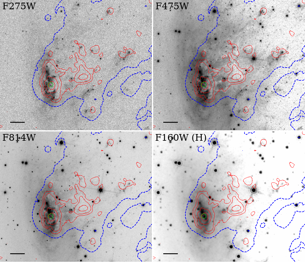
Figure 3: The central regions of the galaxy in the four HST bands. One can see strong dust features downstream of the galaxy (vs smooth light distribution upstream) and enhanced SF in the central part of the galaxy. The dashed blue contour is the outer H$\alpha$ edge from the full MUSE mosaic image (Sun et al., 2022), which shows the stripping front in the galaxy. The red contours show the CO emission from Jáchym et al. (2019). There is a large CO clump downstream of the galaxy, at $\sim$ 2.3 kpc from the nucleus where dust attenuation is significant (especially apparent in the F475W image) and lacks bright star clusters and strong H$\alpha$ emission. This downstream region may be the “deadwater” region, or the stagnant part of the wake that is close to the moving body. Other smaller CO clumps are typically around young star complexes. The green circle (with a radius of 0.5^′′) shows the nucleus. The scale bar is 1 kpc.

We quantitatively examine the galaxy structure by deriving the surface brightness profiles in all four bands along the major axis, minor axis and in elliptical annuli centered at the nucleus (Fig. 4). The galaxy center is set at the nuclear position defined in Section 3.3. The major axis has a position angle of $9.0^{\circ}$ (measured counterclockwise from North). The total F160W light measured from the galaxy is 13.16 mag (without correction from intrinsic extinction) and the half-light radius is $4.91\pm 0.05$ kpc in F160W. This half-light radius in F160W can also be compared with the half-light radius of 4.74 kpc and 4.58 kpc at $B$ band and $I$ band respectively from the SOAR data (S07). It is noteworthy that ESO 137/̄002 (Laudari et al., 2022) is 5.2 times brighter than ESO 137/̄001. However, due to ESO 137/̄002’s bright, central bulge, the half light size of ESO 137/̄002 is approximately 2/3 the size of ESO 137/̄001.

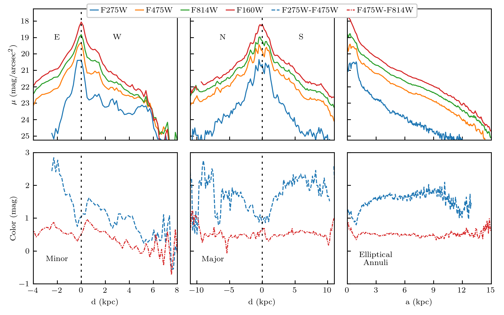
Figure 4: Top-Left: The surface brightness profiles of ESO 137/̄001 along its minor axis (a 6^′′ width and a 0.5^′′ step size). The vertical dashed line shows the position of the nucleus (also the same for other panels in this figure). The east (E) region is upstream because the major axis of the galaxy is almost NS. One can clearly see the upstream-downstream asymmetry especially in UV and blue bands. Note that the bin width is doubled for distances greater than 5 kpc from the nucleus. Top-Middle: The surface brightness profiles of ESO 137/̄001 along its major axis (a 3^′′ width and a 0.5^′′ step size). One can see the light profiles along the major axis are much more symmetric than those along the minor axis. Note that the bin width is doubled for distances greater than 5 kpc from the nucleus. Top-Right: The radial surface brightness profiles of ESO 137/̄001 in elliptical annuli (with the same proportions as the elliptical galaxy region in Fig. 6). The $x$-axis represents the semi-major axis. Bottom Row: The F275W - F475W and F475W - F814W profiles in the relevant regions from the upper panels.

The light profiles along the minor axis are shown in Fig. 4. The profiles are measured in a series of rectangle regions each with a width of 40^′′ and a step size of 0.5^′′. Likewise, the profiles along the major axis are also shown. The profiles are measured in a series of rectangular regions each with a width of 20^′′ and a step size of 0.5^′′. The elliptical profiles are measured in annuli with a width of 0.15^′′ along the major axis and have an axis ratio of 0.44. It is worth noting the asymmetry of the F275W profile along the minor axis (Fig. 4, top-left). The profile shows the faintness of the ultraviolet light in the galaxy upstream regions and an excess of ultraviolet light in the downstream. Since dust in the galaxy is mainly in the downstream region, the intrinsic E-W contrast on the F275W - F475W color is in fact larger than shown in Fig. 4. This demonstrates the quenched SF upstream and enhanced SF downstream in the near tail. The radial profile also shows an F275W-F475W color gradient (Fig. 4, bottom-right) where the galaxy is bluer in the central regions than it is in the outer regions. The F475W-F814W color profiles (Fig. 4, bottom row) shows little change along each axis in these wide bins.

We also derive the structural parameters of ESO 137/̄001 in the F160W band (least affected by intrinsic extinction) using the two dimensional fitting algorithm GALFIT (Peng et al., 2002). For this case, we used a single Sérsic model, as well as a double component model (bulge fitted by a Sérsic model while disk fitted by an exponential component) to fit the galaxy image. The fitted parameters are listed in Table 3. In the case of a single Sérsic model, there is a degeneracy between the Sérsic index and the effective radius. A double component model also fits the F160W image reasonably well. However, as shown in Fig. 1 and Fig. 3, there is no clear evidence for the existence of a bulge. The fits also suggest that any bulge component, if it exists, must be small. We note that both the total F160W light and the half-light radius from profile fitting (Table 1) are similar to the double Sérsic model results with GALFIT (Table 3). Overall, the derived Sérsic indexes are in good agreement with results from large surveys like GAMA (e.g., Lange et al., 2015) for galaxies similar to ESO 137/̄001. Based on the light profiles and the GALFIT results (Table 3), we measure the inclination angle of ESO 137/̄001 to be 66^∘ with the classic Hubble formula (assuming a morphological type of SBc), which is the same as the result from HyperLeda (Makarov et al., 2014). As the motion of ESO 137/̄001 is towards the east and mostly on the plane of sky, we conclude that the near side of the galaxy is towards the east, as the stripped dust clouds need to be located between the disk and us the observer to make the downstream dust features significant. Another way to conclude the east side as the near side is from the spiral arm winding (Fig. 5). As almost all spiral arms are trailing, ESO 137/̄001’s spiral arms are rotating counter-clockwise. As the south side of the galaxy is rotating away from us relative to the nucleus (Fumagalli et al., 2014), the east side must be the near side.

Table 3: The GALFIT fits results for F160W image of ESO 137/̄001

Parameter	Single	Double
	($\chi_{\nu}^{2}$=5.323/6.293)	($\chi_{\nu}^{2}$=5.206)
		Bulge-Sérsic	Disk-Exp
Total mag	12.68/13.78	15.77	13.34
$r_{e}$ (kpc)	9.78/2.74	0.91	5.52
Sérsic index	2.97/(1.0)	1.02	(1.0)
Axis ratio	0.436/0.469	0.351	0.468
PA ($\deg{}$)	8.81/8.22	14.3	5.59

Note: The axis ratio is the ratio between the minor axis and the major axis. The position angle is measured relative to the north and counter-clockwise. For the single Sérsic model, the fit with the index fixed at 1.0 (for an exponential disk) is also shown. Parameters in parentheses are fixed.

3.2 Dust Features

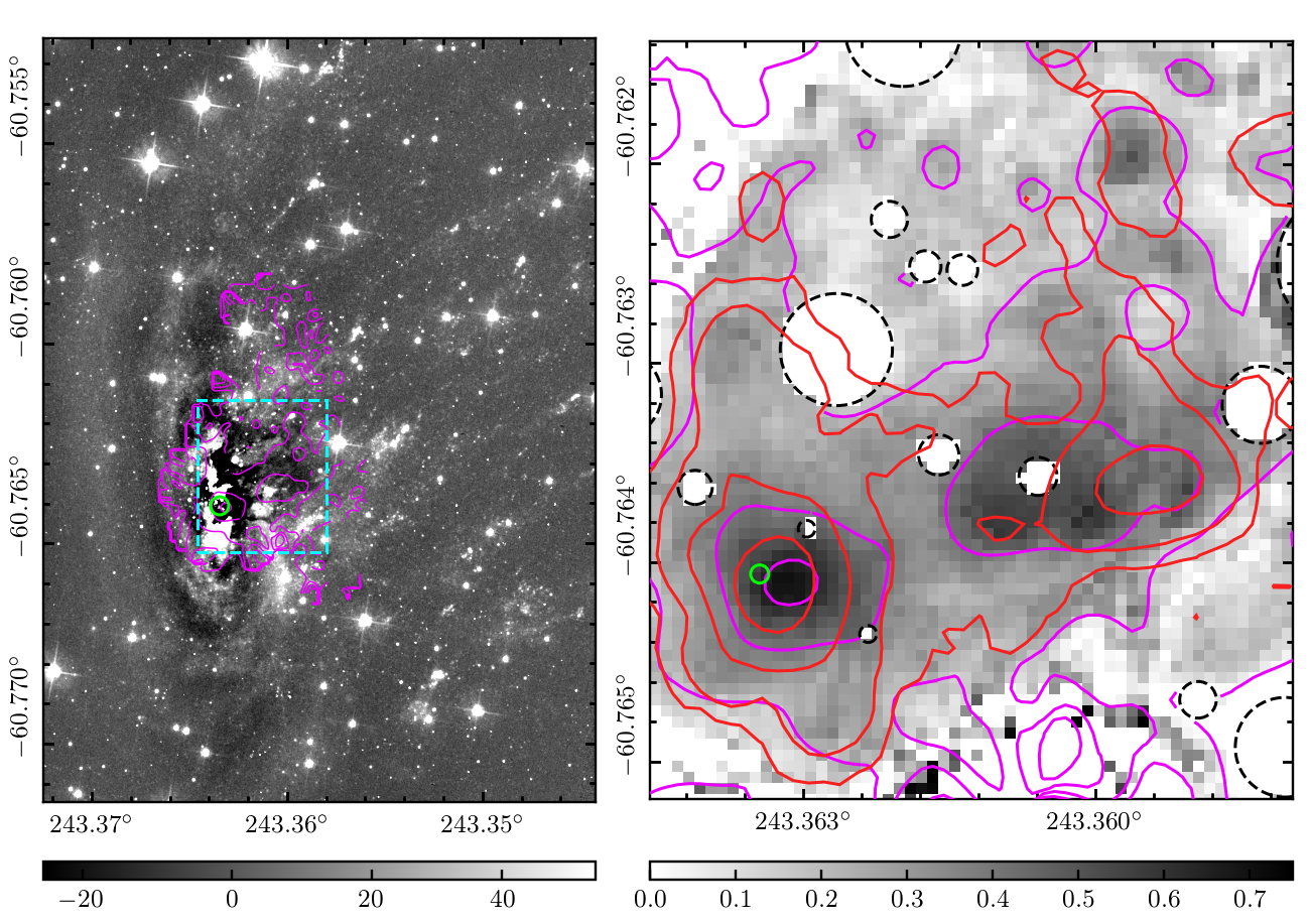
Figure 5: Left: The residual F475W image of ESO 137/̄001, after subtracting the one-Sérsic model fit obtained with GALFIT (Table 3). Spiral arms, dust features downstream of the galaxy and some blue streams composed of young stars can be seen. The galactic nucleus (see Section 3.3) is marked with the small green circle in both panels. The footprint of the E(B-V) image on the right is indicated by the cyan rectangle. Right: The E(B-V) map around ESO 137/̄001, derived from the Balmer decrement with the MUSE data (see Section 3.2), assuming the Calzetti et al. (2000) extinction law. The magenta contours (present in both panels) represent the derived E(B-V) values of 0.0, 0.2, 0.4, and 0.6. The red contours show the CO emission from Jáchym et al. (2019) as shown in Fig. 3. Bright foreground stars were masked in dashed-line circles. One can see a general good correlation between dust features, high extinction regions and CO clouds.

To better show the dust features in the galaxy, we also used GALFIT to produce a residual image with a single Sérsic model in the F475W image. Prior to the analysis, foreground stars are masked. The residual image is shown in Fig. 5. It shows some prominent dust features downstream of the galaxy (also see Fig. 3). The spiral pattern of the galaxy is also better shown after a smoothed component removed. Some dust features downstream of the galaxy can also be seen clearly.

As MUSE has fully covered the galaxy and the tail (Luo et al., 2022), we can use the Balmer decrment to constrain the intrinsic extinction. Our analysis is similar to the work done in Fossati et al. (2016) but with the new data. The stellar spectrum has also been subtracted in the analysis (see Luo et al. 2022 for detail). The Calzetti et al. (2000) extinction law is assumed. The resulting E(B-V) map close to the galaxy is shown in Fig. 5-right. The map shows a region of high extinction a few arcseconds west of the galaxy nucleus with an additional area of high extinction near the CO clump shown by the ALMA data (Jáchym et al., 2019). The MUSE extinction map also shows reasonable correlation to the GALFIT residual image in Fig. 5-left.

3.3 Nucleus

There is no evidence for an active galactic nucleus (AGN) in ESO 137-001 from X-ray, optical, NIR/MIR and radio (Sun et al., 2007; Sun et al., 2010; Sivanandam et al., 2010; Fossati et al., 2016), which makes the identification of its nuclear region not straightforward. We constrain the position of the nucleus from the peaks of the X-ray, H$\alpha$, CO emission in the galaxy (Sun et al., 2010; Fossati et al., 2016; Jáchym et al., 2019), and the GALFIT fits to the HST images, as all these peak positions are consistent with each other within $\sim 1^{\prime\prime}$. The nucleus position is then determined by averaging these positions at (16:13:27.231, -60:45:50.60) with an uncertainty of 0$\aas@@fstack{\prime\prime}$5. There is strong SF ongoing around the nucleus and the nuclear region still retains a lot of molecular gas.

4 Young Star Complexes in the Tail

4.1 Regions of Interest and Source Sample

While S07 defined a sample of H ii regions in the tail of ESO 137/̄001 from the SOAR narrow-band imaging data, the recent full MUSE mosaic (more detail in Sun et al., 2022; Luo et al., 2022) provides much better data to select H ii regions. We selected H ii regions from the extinction-corrected MUSE H$\alpha$ surface brightness map with SExtractor. Sixty-four candidates are identified by selecting for CLASS_STAR $>$ 0.8 (point-like sources) and the ellipticity ($e$) $<$ 0.55. We relaxed the criteria on $e$ (Fossati et al. 2016 used $e<0.2$) as several H ii regions are mixed with the stripped H$\alpha$ filaments, which will enhance the ellipticity obtained by SExtractor. We further applied a limit for the integrated H$\alpha$ flux of the candidates as $2.1\times 10^{-16}$ cm^-2 erg s^-1 to avoid the selection of faint H$\alpha$ clumps in the tail. In addition, the [N ii]/H$\alpha$ emission-line ratio was also required to be less than 0.4 to confirm the ionization characteristic of the H ii candidates. We finally selected 43 H ii regions in the stripped tail of ESO 137/̄001. As shown in Fig. 6, 42 of them are covered by the F275W data, while the other one is just off the F275W field of view (FOV) but covered by the F475W/F814W data. S07 presented a sample of 29 H ii regions, plus 6 more candidates. 27 of these 29 sources are also selected by MUSE. The other two are also shown as compact H$\alpha$ sources in the MUSE data. They would have been selected with a lower flux limit than what was adopted. For the 6 candidates in S07, 3 are MUSE H ii regions. Two others are also shown as compact H$\alpha$ sources but fainter than the chosen threshold. One is not confirmed with the MUSE data. This comparison shows the robustness of the H ii regions selected in S07. The new MUSE H ii region sample also adds 13 new H ii regions compared with S07. These new ones are typically fainter than H ii regions selected by S07 and they are generally close to bright stars. The S07 selection is essentially based on H$\alpha$ equivalent width (EW) so these faint ones that are close to bright stars were not included in S07. Fossati et al. (2016) selected a sample of 33 H ii regions with the 2014 MUSE data that has less coverage of the tail and are also shallower around the galaxy. Thirty two of them are also in the H ii sample of this work. The only one missing has a CLASS_STAR of 0.76 with the now deeper data than what Fossati et al. (2016) used, just below the threshold we adopted.

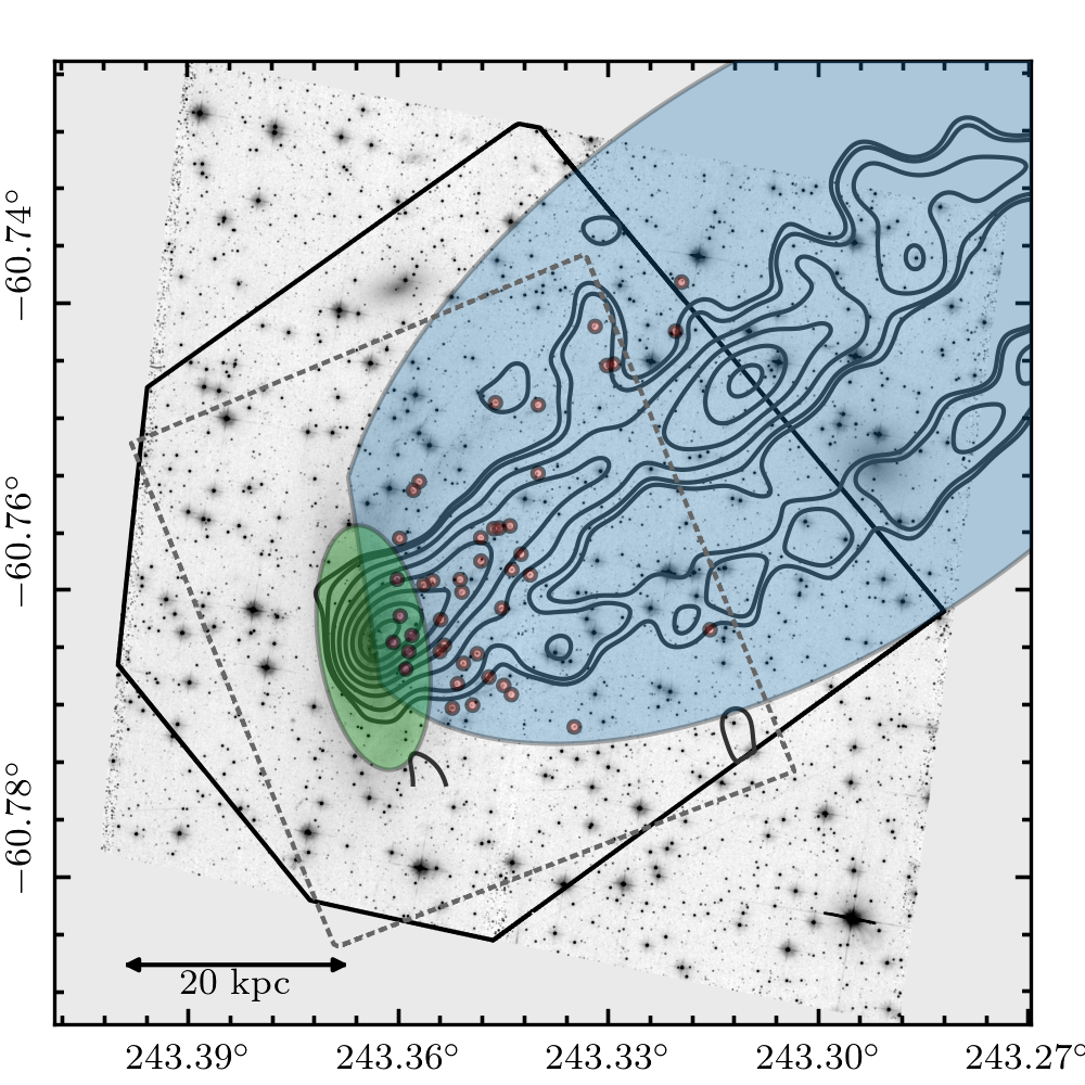
Figure 6: Regions of interest to be studied in this paper are shown here using the F475W image as a reference. The small, red circles denote the 43 H ii regions identified from the full MUSE data (see Section 4.1). The green ellipse centered at the nucleus defined in Section 3.3, angled at $9.0^{\circ}$ from the North and with with semi-axes ($31\aas@@fstack{\prime\prime}{}00$, $13\aas@@fstack{\prime\prime}{}64$), defines the galaxy region. The galaxy region also excludes the six H ii regions that fall in the green ellipse. We also measure the photometry of the galaxy region in 14 smaller regions in 7 radial bins, with each bin divided into the upstream and downstream portions. The largest, blue ellipse indicates the tail regions and is defined by an ellipse centered at (16:13:12.1968, -60:44:36.495) rotated to $34.7^{\circ}$ above the RA axis with axes ($137\aas@@fstack{\prime\prime}{}137$, $72\aas@@fstack{\prime\prime}{}560$). The exception to this tail region is that we exclude the upstream sources which are defined as anything to the east of the major axis of the galaxy, as well as the galaxy region and H ii regions. The control region is therefore defined as the area outside the tail and galaxy regions. Note that our analysis is limited to the field covered by F275W, F475W and F814W observations together, which is marked by the solid, black line. The smaller dotted, gray line indicates the WFC3/F160W FOV. Finally, the gray contours show the Chandra X-ray emission reported in Sun et al. (2010). Only the near part of the $\sim$80 kpc X-ray tail is covered by HST.

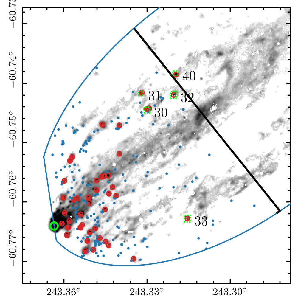
Figure 7: The H ii (red) and blue tail sources (blue) plotted in Fig. 6 are shown on the MUSE H$\alpha$ image from Sun et al. (2022). The solid black line again indicates the field covered by F275W, F475W, and F814W, as shown in Fig. 6. The galaxy nucleus is marked with a green circle on the left. The missing zoom-in regions from Fig. 1 are plotted using green dashed squares.

With the H ii regions defined from the MUSE data, we define four regions of interest (Fig. 6) for the subsequent analysis: small red circles — MUSE H ii regions defined in this work (each represented by a circle with a radius of 1$\aas@@fstack{\prime\prime}$4); the green ellipse — the galaxy region; the large blue ellipse (but within the thick black line to show the common FOV of the F275W, F475W and F814W data) — the tail region; the area outside of the green and blue ellipses but still within the thick black line — the control region. There is common area shared by different regions so it is defined that the galaxy region is the green ellipse excluding small red circles. The tail region is the blue ellipse (but within the thick black line) excluding green ellipse and small red circles. The sky areas for each of the four regions after removal of bright stars are 0.065, 0.313, 3.123, and 2.001 arcmin² for the H ii, galaxy, tail, and control regions, respectively.

For the HST photometry studies of individual sources, we define the baseline sample of sources as sources covered by the F275W, F475W, and F814W data. The baseline source selection is defined as follows. First, spurious sources from wrong alignment, scattered light from bright stars and residual CRs close to the edges were removed. This leaves 3803, 12293 and 10783 sources in F275W, F475W and F814W respectively with SExtractor. Second, only sources detected in at least two adjacent bands were kept. This includes sources detected in all three bands, sources detected in F275W and F475W, and sources detected in F475W and F814W. From this selection, 713 were detected in all three bands, 144 were detected in F275W/F475W, and 4882 were detected in F475W/F814W. After taking the union of these three sets, 5739 sources remain. Third, stars in the the GSC2 catalog (Lasker et al., 2008) were removed. The number of sources was dropped to 5422. Fourth, sources that were brighter than 19.45 mag in F475W, 20.40 mag in F814W, and 21.1 mag in F160W were removed. The F475W magnitude cuts are one magnitude brighter than the brightest star cluster in ESO 137/̄001 and its tail while the F814W and F160W cuts were chosen based on the color-magnitude diagram discussed in section 4.4. Fifth, red sources with F275W-F475W $>$ 2.90 mag and F475W-F814W $>$ 2.00 mag are removed (see Fig. 8 for the corresponding ages). The above two steps decreased the source number to 908. Sixth, sources with individual mag error greater than one mag were removed, which further decreased the source number to 520. This final sample includes 127 in the H ii regions, 201 in the tail, 140 in the galaxy and 36 in the control region. The sources defined in the baseline sample are shown in Fig. 7 which presents the sources identified in the H ii regions in red and other sources identified within the tail.

4.2 Color - Color diagram

We present the color-color (F475W-F814W versus F275W-F475W) results of this baseline sample in Fig. 8 to determine the characteristics of the young star complexes in and around ESO 137/̄001. The figure presents a large number of sources that meet the above criteria within the H ii and tail regions and, a smaller number of sources within the galaxy and control regions. However, the kernel density estimations (KDEs) suggest that the galaxy has a higher number of sources per square arcminute than the tail.

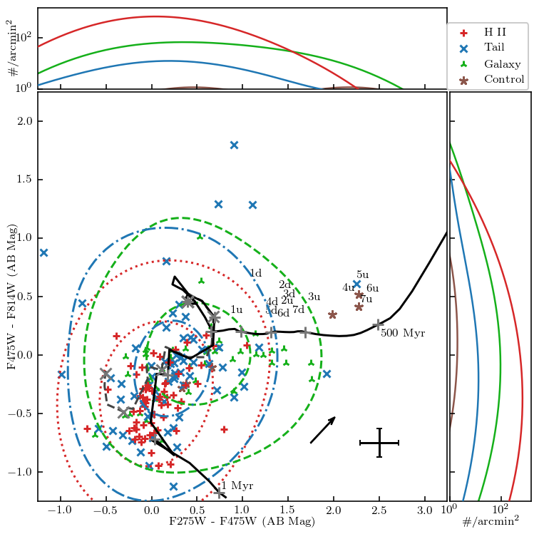
Figure 8: The colors of the HST sources detected in the regions defined in Fig. 6. Sources displayed here were detected in all three bands. Only sources with a photometry error of less than 1 AB magnitude in each filter were selected for studies here. The line plots on the top and right of the figure are the Gaussian KDEs ($\sigma=0.497$ AB mag which is median combined error of the data) of the three band detections that have been normalized by the search area of each region (see Section 4.1). The displayed number of sources for the H ii, tail, galaxy, and control regions are 65, 67, 43 and 6, respectively. The median error of all displayed sources is plotted in the bottom-right of the main figure. The text markers represent each of the seven radial upstream/downstream galaxy sub-regions defined in Fig. 6 where the number in each annotation represents the radial bin (“1” at the nucleus) and the “u” and “d” represent the upstream and downstream regions, respectively. The Starburst99 + Cloudy track (the solid, black line) is superposed. The Starburst99 track is the Genv00 model with $Z=0.014$. The ticks (which are more clearly labeled in Fig. 9) on each track represent ages of 1, 3, 5, 7, 10, 30, 50, 100, 200, and 500 Myr (1 Myr with the bluest F475W - F814W color as marked and 500 Myr at the other end). The gray dashed line at ages of less than 10 Myr represents the track with the Starburst99 model only. An intrinsic extinction value of $E(B-V)=0.08$ (see Section 4.3 for detail) has been applied to the tracks according to the Calzetti et al. (2000) extinction law. The arrow on the figure shows this $E(B-V)=0.08$ extinction effect on the track. We also show the 7.5% and 25% KDE contours for all sources in these three regions (detections plus limits, see Fig. 9 for more details).

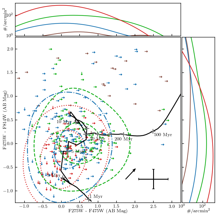
Figure 9: Similar to Fig. 8 but limits on colors are shown. Sources with a right arrow were detected in F475W and F814W but not F275W. Sources with a down arrow were detected in F275W and F475W but not in F814W. No genuine sources detected in F275W and F814W but not in F475W were identified. Otherwise the source selection is the same as Fig. 8. We also show the same KDE contours for all sources (three band detections plus limits) as shown in Fig. 8. The total number of sources for the H ii, tail, galaxy, and control regions are 127, 201, 140 and 36, respectively. The F275W-F475W median errors for each region are 0.20, 0.47, 0.52, and 0.70 AB magnitudes, and the F475W-F814W median errors are 0.15, 0.26, 0.20, and 0.16 AB magnitudes, for H ii, tail, galaxy and control regions respectively. The median error of all sources is plotted in the bottom-right of the main figure. The track is the same Starburst99 + Cloudy track shown in Fig. 8. The line plots on the top and right of the figure now show the Gaussian KDEs for detections plus limits.

Fig. 8 also indicates that the majority of sources in the H ii regions tend to be bluer than those in the galaxy. While there is some overlap between the two sets, the two are distinct regions on the color-color diagram. The sources in the H ii and tail regions are also bluer than the sources in the control region. We also compared the KDE of the H ii and tail regions in Fig. 8. The high source number density in the H ii regions is mainly from its small area by definition. After removing the background contribution estimated from the control region, there are only $\sim$ 18% more sources in the tail region than in the H ii regions and it is also found that sources in the H ii and tail regions have very similar color distributions, which suggests them both as young star complexes. We also show limits (or two-band detections) in Fig. 9 as some of them can be low-mass young star clusters (lacking F814W detection) or older star clusters (lacking F275W detection) in the tail.

4.3 Comparison with SSP tracks

Fig. 8 and Fig. 9 also compares the colors of the HST sources to a Starburst99 (Leitherer et al., 1999) track. Particularly, the Genv00 model (Ekström et al., 2012) with an instantaneous burst, a Kroupa (2001) initial mass function (IMF) and $Z=0.014$ is assumed. While in principle we can use the color-color relation in combination with the simple stellar population (SSP) track to constrain the age of young star complexes, intrinsic extinction in young star complexes needs to be corrected first. We can determine the intrinsic extinction in H ii regions defined from the MUSE data, with the classic Balmer decrement method (e.g., Fossati et al., 2016). As shown in Fig. 10, the median $A_{\rm V}$ is 0.78 mag for 33 H ii regions. If the six regions in the galaxy region are excluded, the median $A_{\rm V}$ is 0.72 mag. If the same extinction law as used in Poggianti et al. (2019) is instead used, the $A_{\rm V}$ decreases by $\sim$ 9%. Thus, the median $A_{\rm V}$ of H ii regions in ESO 137/̄001’s tail is comparable to the median value of 0.5 mag found in the star-forming clumps in the tails of gas stripping phenomena galaxies (Poggianti et al., 2019).

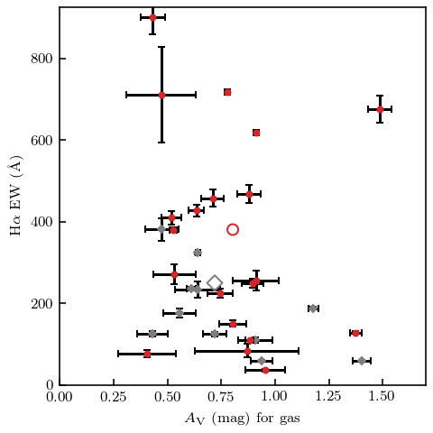
Figure 10: The H$\alpha$ EW vs. the intrinsic extinction $A_{\mathrm{V}}$ for 33 H ii regions. To derive the H$\alpha$ EW, we accounted for the different intrinsic extinction for gas and stars, E(B-V)_star / E(B-V)_gas = 0.44, as discussed in Section 4.3. Sources with MUSE stellar contamination or an unreliable H$\beta$ measurement were removed. The grey points are H ii regions where bright stars are detected in HST within 1.5^′′. The MUSE spectra of these H ii regions have elevated continuum from bright stars so the H$\alpha$ EW is under-estimated, while the $A_{V}$ results are still valid. The 21 red points are H ii regions without bright stars within 1.5^′′ in HST. The large, open gray diamond shows the median values (EW=236 Å and $A_{V}$=0.78 mag) for all 33 sources, while the large, open red circle shows the median values for red points (EW=381 Å and $A_{V}$=0.80 mag). The median EW values are 171 Å and 217 Å, respectively, when the 0.44 factor is not applied.

With the intrinsic extinction of these H ii regions constrained, we can compare their HST colors with the SSP track, which is done in Fig. 11 as discussed in the following. For each H ii region, since colors of nearby HST sources tend to be similar (see Section A.2 and Fig. 20), and considering MUSE’s much lower angular resolution than the HST images, we combine all HST sources within the aperture to derive the colors of the total light. The left panel of Fig. 11 shows the HST colors of the H ii regions, without the correction for the intrinsic extinction. The comparison with the SSP tracks shows, not surprisingly, that the observed colors (especially F275W - F475W) are generally too red, as it is expected that most of these H ii regions are younger than $\sim$ 7 Myr.

Figure 11: Colors of MUSE H ii regions on the Starburst99 track (dashed line) and the Starburst99 + Cloudy track (solid line) with different intrinsic extinction values. In each of the three plots, the scatter points in orange represent the combined photometry for all the HST sources detected in each H ii region. The median, minimum and maximum errors on each of these scatter points is 0.14, 0.04 and 0.73 AB magnitude, respectively. Each plot also contains a Starburst99 track (gray, dashed line) created with the Genv00 model (Ekström et al., 2012), a Kroupa (2001) IMF and $Z=0.014$. The ticks on each track are the same as those in Fig. 8. Likewise, the Starburst99 + Cloudy track is presented as solid, black line. The big cross in each panel is the median uncertainty for the source colors, with different values of extinction adopted. Left: No intrinsic extinction is applied on the colors of the H ii regions. Middle: The intrinsic extinction, determined from the MUSE spectra of nebular emission, is applied on individual H ii region. Right: The same intrinsic extinction as used in the middle panel, but with a stellar-to-nebula extinction ratio of 0.44 (Calzetti, 1997), is applied on individual H ii regions. This choice of intrinsic extinction provides the best match between the HST colors and the model. This plot also shows that the blue star clusters detected by HST are indeed young with ages of $<$ 10 Myr.

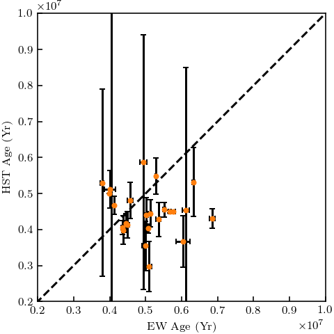
Figure 12: The SSP age derived from the H$\alpha$ EW vs. the SSP age derived from the HST broad-band colors as shown in Fig. 8. Both sets of age estimates were predicted using the Starburst99 + Cloudy model. We limit the comparison to H ii regions without bright stars within $1\aas@@fstack{\prime\prime}{}5$. The best-fit relation is close to the unity line that suggests a general good consistency between these two age estimates, given the current uncertainty.

It should be noted that the Starburst99 SSP models do not include nebular emission from the warm and ionized gas, which can be significant for young stellar populations (e.g., age $<$ 10 Myr). We ran the development version of the photoionization code Cloudy, last reviewed by Ferland et al. (2017), to add nebular emission to the stellar component of the radiation field reported by Starburst99. Cloudy does a full ab initio simulation of the emitting plasma, and solves self-consistently for the thermal and ionization balance of a cloud, while transferring the radiation through the cloud to predict its emergent spectrum. We assumed a nebula of density 100 cm^-3, and metallicity of 0.7 solar, surrounding the stellar source and extending out to 1 kpc from it. For the inner radius of the cloud, we experimented with two values (1 pc and 10 pc), but found that the predicted colors do not depend on that choice. We also imposed a lower limit of 1% on the electron fraction to let the calculation extend beyond the H ii region, into the photo-dissociation region. The Cloudy modification is only important for star clusters younger than 10 Myr (Fig. 11) but does help to explain the F475W - F814W color for some sources. The inclusion of the nebular lines and continuum affects the F475W flux the most and the F275W flux the least.

The middle panel of Fig. 11 shows shows the colors of H ii regions, after the correction for the intrinsic extinction derived from the MUSE data. The same tracks as on the left panel, Starburst99 and Starburst99 + Cloudy, are also plotted. While this comparison does suggest these H ii regions are young (e.g., age $<$ 7 Myr), the F275W - F475W colors are typically too blue.

One way to alleviate this discrepancy is to consider the extinction difference between stars and nebulae. It has been known that the measured extinction on the stellar light can be different from the measured extinction on the warm gas (e.g., Calzetti et al., 1994; Calzetti, 1997; Koyama et al., 2019). Calzetti (1997) gave an average relation of E(B-V)_star / E(B-V)_gas = 0.44 (also see Calzetti et al., 1994, 2000). This difference may suggest the spatial decoupling of the ionized gas and the young stellar population and other geometry effects (e.g., Calzetti et al., 1994; Charlot & Fall, 2000). There have been some works to study the relation between this ratio and specific star formation rates, redshift and stellar mass (Wild et al., 2011; Wuyts et al., 2011; Price et al., 2014; Reddy et al., 2015). Most recently, Koyama et al. (2019) has shown that this ratio generally increases with increasing specific star formation rate while it decreases with increasing stellar mass, although the scatter is substantial. In this work, we simply apply the ratio of 0.44 as suggested by Calzetti (1997). With this factor included, as shown in the right panel of Fig. 11, the match between the HST colors and the Starburst99 + Cloudy model is improved.

To summarize, we include two corrections, adding nebular emission from Cloudy and considering the different extinction for stars and gas, to alleviate the initial discrepancy between the HST broad-band colors and the SSP tracks. Given the uncertainty on the HST colors, the intrinsic extinction on young stars, the Balmer decrement and the Starburst99 models, the colors of these H ii regions are consistent with the expectation for young stellar populations at age of $<$ 10 Myr. Therefore, in this work, we simply adopt an intrinsic extinction of $E(B-V)=0.08$ for all the HST sources in the tail. This value is derived from $0.44A_{\mathrm{V}}=E(B-V)k_{\mathrm{V}}$ where $A_{\mathrm{V}}=0.72$ mag from the MUSE data, $k_{\mathrm{V}}$ is calculated according to the Calzetti et al. (2000) law with $R_{\mathrm{V}}=4.05$. Fig. 8 then compares the colors of the HST sources to these tracks.

We also compare the age determined from the HST broad-band colors with the age determined from the H$\alpha$ EW especially since the EW is not affected by the intrinsic extinction. The Starburst99 model gives the direct relation between the SSP age and the H$\alpha$ EW. Using the same model and the associated track in Fig. 11, we also predicted the age of sources using the HST colors. The age was determined by matching the colors of sources in Fig. 11-right to the track using the shortest euclidean distance. The age error is estimated from Monte Carlo simulations with the errors of colors considered. As shown in Fig. 12, the consistency between two age estimates is generally good, when we only include H ii regions with robust EW measurements. The best-fit relation is also close to the unity line. Thus, with all the uncertainty discussed above, we conclude that the HST broad-band colors can present good constraints of the SSP age.

4.4 Properties of the HII regions

We also analyzed the correlation between the source distance from the major axis of the galaxy and the color of that source. Fig. 13 (left) shows that there is no strong evidence for the change of the F275W - F475W color with the distance to the galaxy, with the large scatter of the colors observed.

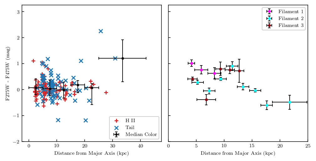
Figure 13: Left: The F275W - F475W color vs. distance relation for a subset of sources in the H ii and tail samples established in Section 4.2. We restrict the sources to have an error of less than 0.4 mag here rather than 1.0 mag as in Section 4.2. The median colors plotted include both H ii and tail sources. The $x$ error bars indicate the bin size and the $y$ error bars indicate the 1-$\sigma$ scatter in the bin. There is no clear change on the average source color with the distance to the galaxy. Right: The same relation for three different filaments extending from ESO 137/̄001. Filament 1 corresponds to the filament with regions 25 and 26 in Fig. 1, Filament 2 corresponds to the filament with regions 23 and 27-30 in Fig. 1, and Filament 3 corresponds to the filament with regions 17, 18 and 21 in Fig. 1. Although the uncertainties are still large and the intrinsic extinction is not applied, at least two filaments become bluer further away from the galaxy.

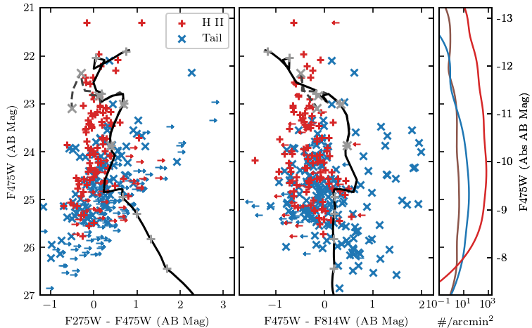
Figure 14: The color-magnitude diagram for the sources in the H ii and tail regions, with the absolute magnitude also shown on the right side. The same tracks as in Fig. 11 are also shown (for a total mass of $10^{4}$ M_☉). The markers on tracks are also the same (note star clusters become dimmer as they get older so small ages start from the top). From these tracks, the mass of these young star complexes is $10^{4}$ - $10^{5}$ M_☉ if younger than $\sim$100 Myr.

Fig. 13 (right) shows the color along three different blue filaments within the tail. This approach was chosen to ensure no information was lost in the ensemble method shown in Fig. 13 (left). All light within the filament regions (less the bright foreground sources) is integrated for this second figure to see how the color changes along an individual filament. Although it is not significant, there is a slight trend from red to blue for filament 1 as the distance increases. Filament 3 has an interesting discontinuity where the color goes from blue to red then to blue again as the distance increases.

We also present the Color-Magnitude diagram in Fig. 14 which gives us a constraint on the masses of the young star complexes if the age is determined from e.g., the color-color diagram. The color-magnitude diagram suggests that the young star complexes have a mass of $10^{4}$-$10^{5}$ M_☉ if younger than $\sim$100 Myr (see more detail regarding mass calculations in Section 5.2). The diagram on the left also delineates the detection threshold near the bottom, between the F475W magnitude and the F275W-F475W color. The displayed track is the same as the ones used in Fig. 8 and Fig. 11.

The luminosity distribution is presented in Fig. 15. The figure shows H ii and tail sources (see Section 4.1) that were detected in all three bands (red) and F475W/F814W detections + F275W upper limit (light red). We model the data in Fig. 15 according to a luminosity function of $dN/dL\sim L^{-a}$ where $dN$ is the number counted per luminosity bin $dL$, $L$ is the luminosity and $a$ is the power law index. The three band detections (for sources brighter than -9.5 mag) correspond to $a=2.0\pm 0.1$ while the addition of upper band detections correspond to $a=2.3\pm 0.1$.

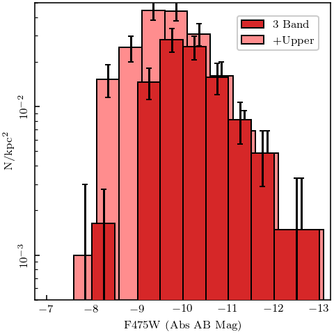
Figure 15: The luminosity distribution for sources detected in the H ii and tail regions defined in Section 4.1 with the exception that a F275W - F475W color cutoff of 2.5 is chosen. The control sample has been subtracted from each distribution. The darker distribution represents the sources detected in three bands whereas the lighter distribution include F275W upper limits. Note that the upper limit distribution has been offset for display only.

4.5 Relationship with the H ii regions and CO sources

To compare the distribution of the young star complexes, the H ii regions, and the CO compact sources, we need to verify the astrometry between HST, MUSE and ALMA. First, we compared the astrometry of the HST images and the MUSE continuum surface brightness map. We select 16 bright stars from the 2MASS point source catalog in the common area of the HST and MUSE fields, which are adopted as the reference stars of the WCS for each field. Then we use the WCSTools package to update the WCS of the HST images and MUSE H$\alpha$ surface brightness map. By comparing the position of the reference stars in each image, we found that the offsets between them are generally (75%) less than the pixel size $0\aas@@fstack{\prime\prime}2$ of the MUSE maps. The rms of $\delta$RA and $\delta$Dec are $0\aas@@fstack{\prime\prime}22$ and $0\aas@@fstack{\prime\prime}05$, respectively, suggesting that the WCS of these two images are well aligned. This first step has already calibrated the absolute astrometry of the HST and MUSE data. Second, we in principle need to compare the astrometry of the MUSE H$\alpha$ surface brightness map and the ALMA CO(2$-$1) intensity map. However, there is not a single common source between the MUSE maps (continuum or lines) and the ALMA continuum map. One also cannot assume perfect matches between ALMA CO clumps and MUSE H ii regions (see Fig. 1). Thus, we rely on the absolute astrometry of the ALMA maps, which should be better than $0\aas@@fstack{\prime\prime}3$ for our data (see the ALMA website on the typical absolute astrometric accuracy of ALMA).

As shown in Fig. 1, the correlation between the HST blue star clusters and the H ii regions is very good, with all MUSE H ii regions having at least one HST blue star cluster within 0.2 kpc. There are many HST blue sources not identified as H ii regions from our criteria but they are typically associated with faint H$\alpha$ clumps. On the other hand, only about a quarter of H ii regions have associated CO clumps within 0.3 kpc, with another quarter having nearby CO clumps beyond 0.3 kpc and half of H ii regions without nearby CO clumps detected at all. Some CO clumps are also not associated with any activity of SF, being H ii regions or the HST blue star clusters, e.g., in zoom-out #11, #16, #22, #34, #35 and #36. Assuming H ii regions and HST blue star clusters are formed out of molecular clouds, the parent molecular clouds may get disrupted quickly after the initial SF. Some molecular clouds probably have not collapsed yet. More detailed studies on the relationship between molecular clouds and young star complexes require detailed studies with the ALMA, MUSE and HST data, which is beyond the scope of this paper.

4.6 Relationship with the Chandra X-ray sources

S10 discovered some X-ray point sources around ESO 137/̄001’s tail with the Chandra data. Some of them were suspected to be associated with young star complexes in the tail. We zoom in around some Chandra sources close to blue star clusters in Fig. 1. Particularly, sources C6, C8, C9, C10, C11 and C12 are close to young star complexes. All of them are downstream and still close to the galaxy. If associated with ESO 137/̄001, they would be ultraluminous X-ray sources (ULXs). The offset between the X-ray source and the young star complexes observed here, typically within several hundred pc, is also normal for ULXs (e.g., Poutanen et al., 2013).

5 Discussion

5.1 Star formation in the galaxy

The total FIR luminosity of the galaxy was derived from the Herschel data. We used the Herschel source catalog, particularly the PACS Point Source Catalog and the SPIRE Point Source Catalog. We used the python code MBB_EMCEE to fit modified blackbodies to photometry data using an affine invariant Markov chain Monte Carlo (MCMC) method (Foreman-Mackey et al., 2013), with the Herschel passband response folded (Dowell et al., 2014). Assuming that all dust grains share a single temperature $T_{\mathrm{d}}$, that the dust distribution is optically thin in the FIR, and neglecting any power-law component towards shorter wavelengths, the fit results in a temperature of $T_{\mathrm{d}}$ = (32.1$\pm$0.5) K, a luminosity $L_{\mathrm{8-1000\ \mu m}}$ = (5.24 $\pm$ 0.12) $\times$ 10⁹ L_⊙, and a dust mass of $M_{\mathrm{d}}$ = (1.3 $\pm$ 0.1) $\times 10^{6}$ M_⊙ for $\beta$ = 1.5. For $\beta$ = 2, $T_{\mathrm{d}}$ = (28.6$\pm$0.5) K, $L_{\mathrm{8-1000\ \mu m}}$ = (5.06 $\pm$ 0.11) $\times$ 10⁹ L_⊙ and $M_{\mathrm{d}}$ = (2.1 $\pm$ 0.2) $\times 10^{6}$ M_⊙. It is noted that the dust temperature in ESO 137/̄001 is higher than those typically found in Virgo cluster galaxies ($\sim$ 20 K, Davies et al., 2012; Auld et al., 2013). Such a high $T_{\mathrm{d}}$ is consistent with the results by Bocchio (2014).

The total SFR of the galaxy is 0.97 M_⊙/yr, from the Galex NUV flux density and the total Herschel FIR luminosity with the relation from Hao et al. (2011). If using the WISE 22 $\mu$m flux density and the relation from Lee et al. (2013), the estimated total SFR is 1.39 M_⊙/yr. The Kroupa initial mass function (IMF)is assumed in both cases. The Lee et al. (2013) work assumed the Salpeter IMF so we multiply its SFR relation by 0.62 to convert to the Kroupa IMF. With the measured molecular gas content of $\sim 1.1\times 10^{9}$ M_⊙ in the galaxy (Jáchym et al., 2014), the gas depletion timescale is $\sim$ 0.9 Gyr. ESO 137/̄001 still appears on the galaxy main sequence with its current SFR and the total stellar mass (Boselli et al., 2022).

The upstream of the galaxy (or the east side, or the near side) is dust free and gas free (Sun et al., 2007; Sun et al., 2010; Fossati et al., 2016) so the current SF is mainly around the nucleus and the downstream. The H$\alpha$ disk is truncated to $\sim$ 1.5 kpc radius, similar to the size of the remaining CO cloud in the galaxy (Fig. 3). More detailed studies of SF history in the galaxy can be done with the MUSE data and multi-band photometry data in the future.

5.2 Star formation in the tail

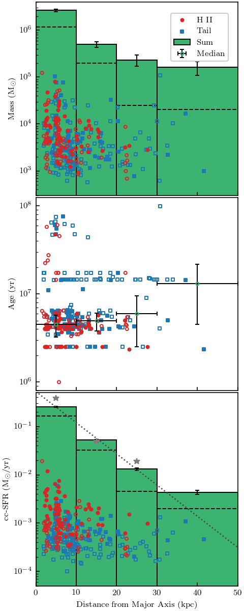
Figure 16: The mass, age, and color-color SFR (cc/̄SFR)for sources younger than 100 Myr as estimated with the Starburst99 + Cloudy model. For the age distribution, the median values (filled markers for three-band detections and empty markers for two-band detections) and 1$\sigma$ scatter are also shown. The histograms in the top and bottom panels represent the median summed masses and cc/̄SFRs of both regions within the respective distance bin, with the uncertainty also shown. The dashed histograms and filled green scatter points are for the same quantities but for the 3 band detections only. The dotted line in the bottom panel shows an exponential fit of the total cc/̄SFR to the source distance (see Section 5.2). The large grey stars in the bottom panel show the total SFR derived from the H$\alpha$ data in the same bin.

Star formation in the tail can be constrained from the H$\alpha$ data. As discussed in Section 4.1, we defined 43 H ii regions in the tail region, including 37 beyond the galaxy region. The total H$\alpha$ flux of each region, within a circular aperture with a radius of 1.4^′′, is measured, after correcting for both the Galactic extinction and the intrinsic extinction. The total H$\alpha$ luminosity for 43 H ii regions is 8.1$\times 10^{40}$ erg s^-1. Excluding the six in the galaxy region, the total H$\alpha$ luminosity is 4.0$\times 10^{40}$ erg s^-1. With the H$\alpha$ — SFR relation from Hao et al. (2011) assuming a Kroupa IMF, the corresponding SFR is 0.45 and 0.22 M_☉/yr, respectively. These SFR values are similar to the estimate from S07 (0.59 M_☉/yr) for 29 H ii regions assuming a Salpeter IMF and $A_{\rm V}$ = 1 mag.

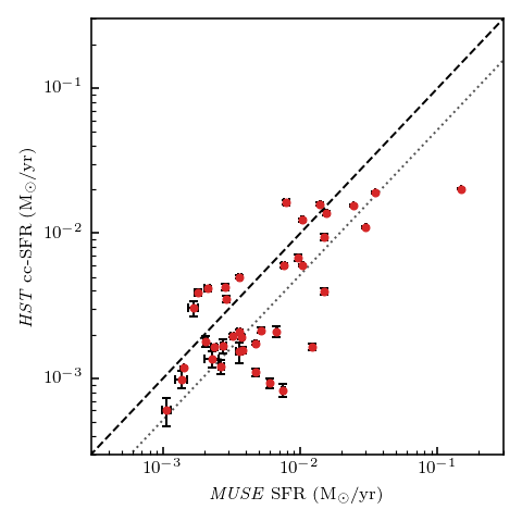
Figure 21: The comparison of the SFR as measured by the MUSE EW and the cc/̄SFR as measured by HST for the H ii regions discussed in Section 4.1 with the exception of four regions where no HST sources were detected. The points represent the median values of the 50,000 Monte-Carlo iterations and the error bars represent the median absolute deviation (see Section 5.2). The dashed line shows the unity line while the dotted line shows the best fit of the ratio of 0.52. The median ratio is 0.61 and the median absolute deviation is 0.24.

Star formation in the tail can also be constrained from the HST broad-band photometry data as discussed in Section 4. We used the Starburst99 + Cloudy model in Fig. 8 to estimate the ages and masses of star clusters. The age was estimated by comparing the F275W-F475W and F475W-F814W colors to the track in Fig. 8, taking the value at the closest distance from the track. This process was performed with a Monte Carlo simulation using 50,000 samples where the F275W, F475W, and F814W magnitudes were assumed to be normally distributed using the measured magnitude as the mean and the measured uncertainty as the standard deviation. Again, the assumed intrinsic extinction is $E(B-V)=0.08$ as discussed before. Once an age is determined, we estimate the mass of the source by matching the F475W magnitude to the corresponding track in the color - magnitude relation in Fig. 14. This is done by assuming the difference in measured F475W magnitude and track magnitude for the matched age is due to the difference in mass. For example, the Starburst99 track in Fig. 8 assumes a population mass of $10^{6}$ M_☉. If a source is 5 mag dimmer in F475W than the age-matched point on the Starburst99 track (after the correction on the intrinsic extinction), the mass is then $10^{4}$ M_☉. Once the age and mass are known, we can estimate the color-color SFR (cc/̄SFR)by dividing the mass by the age and sum up the individual cc/̄SFR values for all sources to get the total cc/̄SFR in each Monte Carlo iteration. If only sources younger than 10 Myr are counted, the median cc/̄SFR is 0.199 M_☉/yr and 0.083 M_☉/yr for the H ii and tail sources, respectively. If instead all sources younger than 100 Myr are included, the cc/̄SFR is 0.210 M_☉/yr and 0.117 M_☉/yr for the H ii and tail sources, respectively. The Monte Carlo uncertainty on these values is 0.7% and 6.4% for the H ii and tail sources, respectively, according to the median absolute deviation. This estimate of the cc/̄SFR for H ii regions is only about half the estimated SFR from the H$\alpha$ data (see Section A.3 and Fig. 21).

The total cc/̄SFR in Fig. 16 was fit to the source distance ($d$) (dark-gray dotted line in bottom panel) according to

$$\mathrm{cc\mbox{--}SFR}=a\exp\left(-d/\delta\right).$$ (1)

The resulting fit gives $a=0.53\pm 0.01$ M_☉ yr^-1 and $\delta=6.7\pm 0.4$ kpc, which again shows the cc/̄SFR in the tail decreases fast with the distance to the galaxy. We also derived the SFR from the H$\alpha$ data in the same spatial bins (Fig. 16). The fit with the same model gives $a=0.89\pm 0.04$ M_☉ yr^-1 and $\delta=5.7\pm 0.6$ kpc. Cramer et al. (2019) noted this trend in D100. This trend is also noted for some other galaxies in RPS (e.g., George et al., 2018; Poggianti et al., 2019; Boselli et al., 2022).

With E(B-V)_star / E(B-V)_gas = 0.44, the total stellar mass in the tail is $\sim 2.7\times 10^{6}$ M_☉. With the above ratio equal to 1, the total stellar mass remains about the same, $\sim 2.9\times 10^{6}$ M_☉. Fig. 16 shows the Monte Carlo median mass, age, and cc/̄SFR for sources less than 100 Myr old as a function of distance from the galactic major axis for the three band and two band young star clusters identified in Section 4.1. Likewise, the graphic shows the median summed masses, median ages, and median summed cc/̄SFRs for four distance bins. The individual sources do not show any significant trend regarding how these properties change with distance. However, the summed and median statistics do show that the total mass and the total cc/̄SFR decrease with distance from the galaxy while the median age of the sources remains nearly constant with the uncertainty. On the other hand, any age trend is limited by our sensitivity to old ($>$ 100 Myr) sources as discussed later in this section. About 95% of SF in the tail is within 20 kpc from the galaxy. The SF beyond 20 kpc is still observed but very weak.

Fig. 16 shows that sources older than 40 Myr are mostly close to the galaxy (within 13 kpc). There is a lack of old sources beyond 15 kpc from the galaxy. There are several factors that can contribute to this result. First, assuming a galaxy total mass of $5\times 10^{10}$ M_☉, the free fall time from 30 kpc to the galactic plane is $\sim$ 350 Myr. Considering, the actual fall-back time to any height above the galactic plane would be some fraction of this value, it is conceivable that some old sources that are close to the galaxy ($<$ 10 kpc) formed further away from the galaxy, but have had sufficient time to fall back toward the galaxy. Second, the intrinsic extinction may be underestimated for some old sources that are close to the galaxy, which would result in over-estimate of their ages. Third, the faint, old (or red) sources have a larger contamination from background sources (see the KDEs in Fig. 8).

Fig. 17 shows the estimated mass for sources younger than 100 Myr as a function of the source age for the three band and two band young star complexes identified in Section 4.1. On the face value, Fig. 17 suggests that most SF in the tail happened within the recent 3 - 10 Myr. However, as sources become fainter when they age, it is clear that the current data present a lower mass detection limit increasing fast with the source age (also evident in Fig. 17). We then derived the empirical mass limit in Fig. 17 to better understand this limitation. The displayed limit is calculated by requiring the error of the F275W - F475W color less than 1 and also assuming the Starburst99 + Cloudy track in Fig. 8 and the median extinction reported in Fig. 10. As shown in Fig. 17, the displayed limit does well to predict the limiting mass at each age helping explain why we do not measure high age / low mass sources. A few sources do exist below this empirical limit, however they tend to be sources detected in two bands (and are therefore likely to not be detected in F275W at all). We fit the mass limit for ages greater than 3 Myr according to a power law with an index of 1.3.

Fig. 17 also reveals a population of young ($<$ 10 Myr) tail sources that are not associated the an H ii region. As shown in Fig. 8, the background contamination for these blue sources is negligible. The total mass of these sources sums to $3\times 10^{5}$ M_☉. However, some of these sources are near H ii regions (see Fig. 7) although they are not in the H ii regions of interest detailed in Section 4.1. We therefore measure the mass of these tail sources that are within 0.7 kpc of H ii regions to be $1.5\times 10^{5}$ M_☉. For the remaining sources, they are typically within 1.2 kpc of the selected H ii regions, especially for bright or massive sources.

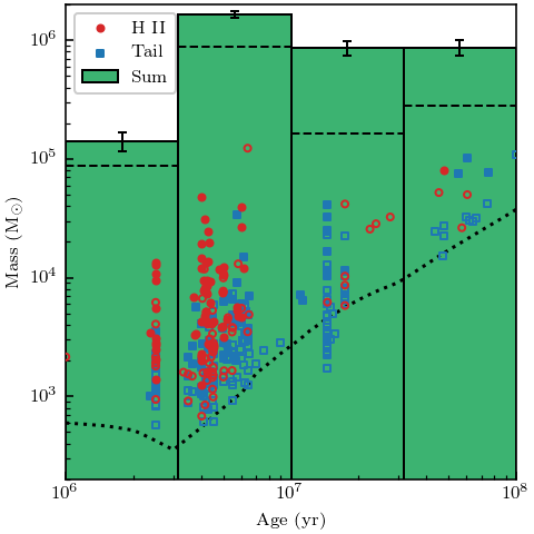
Figure 17: The mass with the source age for sources younger than 100 Myr as estimated with the Starburst99 + Cloudy model. The marker and histogram styles are the same as in Fig. 16. The empirical mass limit that can be reached with our data is shown as the dotted line.

We also present the cc/̄SFR spatial distribution in Fig. 18. The figure highlights a few pockets of higher SF (primarily close to the galaxy center) while the majority of sources only make a small contribution to the total SF. Although not shown in Fig. 18, the mass distribution is nearly identical to the displayed cc/̄SFR distribution.

Fig. 18 also marks the three zones in the tail defined by the H$\alpha$ data from MUSE, north, central and south zones (more detail in Luo et al. 2022). We performed the same analysis for Fig. 16 for each of the tail zones. This further analysis was motivated by the different morphology in each of the three zones. In the north zone, stripping is in an advanced stage as the galaxy region is nearly cleared. H ii regions are detected to the largest distance to the galaxy in this zone. In the south zone, stripping may be in a little less advanced stage than in the north zone, as the south side of the galaxy is more on the leading size to the ICM wind while the north side of the galaxy is more on the trailing side. The majority of H ii regions in the southern zone are within $\sim$ 10 kpc of the galaxy major axis. The remaining sources in this zone tend to have the same mass distribution as the rest of the zone but tend to have a higher age distribution. For the central zone, stripping is still ongoing around the nuclear region from the X-ray, H$\alpha$ and CO data. All H ii regions are within $\sim$ 15 kpc of the major axis. There is a lower density of non-H ii sources within this zone that tend to have the same age as the rest of the sources in this zone, though they do tend to be low-mass. In the end, the results in these separated zones are similar to those in Fig. 16.

One should also be aware of caveats in our analysis in this section. First, our results are only based on the data from three HST photometry bands. Model fitting was done from the color-color diagram, while a more rigorous statistical approach with more photometry bands (e.g., Linden et al., 2021; Moeller & Calzetti, 2022) cannot be performed. Second, the SSP models have their uncertainty (see the recent comparison by Wofford et al. 2016). Third, our results are based on the assumption that each star cluster complex we studied can be reasonably approximated by an instantaneous burst (single) population. Fourth, we only assumed a fixed, average intrinsic extinction. Lastly, when the total mass is less than $\sim$ 3000 M_⊙, the stellar IMF is not fully sampled so the results below this mass limit will have a larger uncertainty. While the more robust stellar population synthesis codes for such low-mass clusters exist (e.g., SLUG from da Silva et al. 2012), many of star clusters in our work are more massive than 3000 M_⊙ and a more in-depth stochastical modeling is beyond the scope of this work.

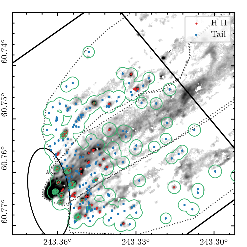
Figure 18: The cc/̄SFR distribution in the tail of ESO 137/̄001 plotted on the MUSE H$\alpha$ image. The green contours are generated using a spatial KDE using the cc/̄SFR of each source as the sample weight. Areas with higher contour value correspond to 1) a higher density of young star clusters and/or 2) regions of high cc/̄SFR. The figure highlights a few pockets of high SF (primarily close to the galaxy center) while the majority of sources only make a small contribution to the total SF. The solid, black lines show the F275W FOV, and the dark-gray dotted lines show the division of the north, central, and southern tail zones from top to bottom. The galaxy region defined in Fig. 6 is shown as the black ellipse.

5.3 Stripping history of ESO 137-001

Figure 19: Four ideal examples of a symmetrical disk galaxy undergoing ram pressure stripping and the observed signature of dust distribution. The LOS is also perpendicular to the paper while the arrow marks the ICM wind direction.

What is the geometry of stripping in ESO 137/̄001? The HST data give the distribution of dust that can constrain the geometry of stripping. Four special examples of a disk galaxy undergoing RPS and the expected signature of dust distribution are shown in Fig. 19. ESO 137-002 is close to case iv (Laudari et al., 2022) and NGC 4921 is close to case ii (Kenney et al., 2015). ESO 137/̄001 has an inclination of $\sim 66^{\circ}{}$ so it is viewed closer to edge-on than face-on. The eastern side of the galaxy is the leading side to ram pressure and is also the near side to us as discussed. If ESO 137/̄001 is moving on the plane of sky, the ICM wind angle with the disk plane is $\sim 66^{\circ}{}$. As ESO 137/̄001 has a small velocity component towards us (relative to the cluster system velocity), the ICM wind angle with the disk plane is less than $\sim 66^{\circ}{}$. Based on the tail direction, Jáchym et al. (2019) estimated an ICM wind angle of $\sim 47^{\circ}{}$, which makes stripping in ESO 137/̄001 about the midway between edge-on and face-on.

What do the HST data inform us on the stripping history of ESO 137/̄001? As discussed in Section 3, dust is detected around the nucleus and the downstream region immediately behind the nuclear region. RPS started from outside of the galaxy and has now progressed into the central region of the galaxy. SF is still ongoing around the nucleus and the downstream region behind the nucleus, as there is still abundant cold molecular gas around the nucleus (Fig. 3). On the other hand, an ideal outside-in model of stripping is too simple. One has to consider the actual distribution of the multi-phase ISM that is often porous so stripping can happen at multiple radii at the same time. The presence of a galactic bar may also cause a relative deficit of gas at intermediate radii. As shown in Fig. 4, the colors along the major axis of the galaxy are mostly constant, while an ideal outside-in stripping and quenching may produce a continuous color gradient, as observed in D100 (Cramer et al., 2019). More detailed analysis on the stripping/quenching in ESO 137/̄001 is required in the future with the optical spectroscopic data from e.g., MUSE.

A detailed inventory study of the ISM in ESO 137/̄001 was done by Jáchym et al. (2014). About 80% - 90% of the original ISM in ESO 137/̄001 has been removed from the galaxy, presumably by RPS. At least half of the removed ISM is accounted for in the tail, mostly in the molecular gas. While more data are required to better constrain the mass the multi-phase gas in ESO 137/̄001’s tail (e.g., H i and improved H$\alpha$ estimates from the MUSE data), the biggest uncertainty seems to be on the diffuse cold molecular gas as the ALMA 12m + ACA data on CO(2-1) still miss $\sim$ 70% of CO flux from the single-dish data by APEX (Jáchym et al., 2019).

6 Conclusions

We present a detailed analysis of ESO 137/̄001, an archetypal RPS galaxy, with the HST ACS and WFC3 data in four filters (F275W, F475W, F814W and F160W).

1. The galaxy has clear, asymmetric light and dust distribution indicative of ongoing RPS (Fig. 1, Fig. 3 and Fig. 4). The eastern side of the galaxy is the near side to us, also the leading side to ram pressure. The stripping is about the midway between edge-on and face-on stripping. The light profile effectively shows that SF has been quenched in the upstream regions and the current SF is mainly around the nucleus and downstream regions. The dust images show stripping near the nucleus of the galaxy where the dust has been pushed to the downstream side of the galaxy. We derived the E(B-V) map (Fig. 5) that shows the strong dust extinction downstream. There is also an enhanced dust feature at $\sim$ 2.3 kpc downstream, corresponding to a large CO clump. We suggest it is around the “deadwater” region. Stripping happens outside-in generally and has progressed into the inner $\sim$ 1.5 kpc radius of the nucleus. There is no evidence for an AGN in ESO 137/̄001 from the HST and X-ray data.

2. HST data reveal active SF in the downstream gas stripped (Fig. 1, Fig. 7 and Fig. 8). We derived the color-color (F275W - F475W vs. F475W - F814W) diagram for sources identified in different regions of interest, including the galaxy, H ii, the tail and the control regions (Fig. 6). The galaxy, tail and H ii regions all show significant excess of blue sources compared with the control region. We conclude these blue sources are young star complexes formed in the stripped ISM and HST can pick up faint young star complexes no longer hosting bright H ii regions.

3. H ii regions in the stripped gas are well correlated with young, blue star clusters but not with CO clumps. As shown in Fig. 1, the correlation between the HST blue star clusters and the H ii regions is very good, with all MUSE H ii regions having at least one HST blue star cluster within 0.2 kpc. Other HST blue sources typically have faint H$\alpha$ clumps associated. On the other hand, only about a quarter of H ii regions have associated CO clumps within 0.3 kpc, while half of H ii regions do not have nearby CO clumps detected at all. Some CO clumps are also not associated with any activity of SF. We conclude that the parent molecular clouds get disrupted quickly after the initial SF. Some molecular clouds are not forming stars at the moment. The comparison between the HST and the Chandra images also suggests up to six ULXs in the tail region.

4. Ages derived for the H$\alpha$ EW are consistent with those derived from the HST broadband colors (Fig. 11 and Fig. 12). We applied a SSP model with Starburst99 on these blue star clusters. For those associated with H ii regions with the MUSE data, we can compare the age derived from the SSP model (or with broadband colors) with the age derived from the H$\alpha$ EW. While the initial analysis shows a significant discrepancy between two estimates, we conclude that these two estimates can be brought back into agreement if 1) allowing different extinction between the nebular and stellar components for young star complexes around H ii regions (particularly we adopted E(B-V)_star / E(B-V)_gas = 0.44 from previous studies); and 2) nebular emission is included in the SSP tracks for ages of less than 20 Myr.

5. The SF history in the tail can be quantitatively constrained from the HST broad band colors. We trace SF over at least 100 Myr and observe a broader spatial distribution of young star clusters than H ii regions only traced by H$\alpha$, and give a full picture of the recent evolutionary history of SF in the tail. We showed that the average mass of the sources detected have a mass of $10^{3}$-$10^{4}$ M_☉ and that the ages of most sources is younger than approximately 100 Myr. We measure the total SFR of the H ii regions to be 0.2 - 0.45 M_☉/yr and other blue sources in the tail region add about 30% more SFR, all for sources younger than 100 Myr. The total SFR in the tail is substantial, about 40% in the galaxy. We measure the total stellar mass in the tail to be $\sim 2.7\times 10^{6}$ M_☉. The H ii and tail regions combined have a luminosity function $(dN/dL\sim L^{-a})$ for $a\approx 2.1$ (Fig. 15).

6. We also examined the F275W - F475W color of selected sources in the H ii and tail regions as a function of distance from the galaxy (Fig. 13) but no trend is found. The trend is also not clear for color changes along blue streams. While naively it is conceivable that the gas furthest from the galaxy was pushed out before the gas near the galaxy, the ages of young star complexes does not indicate this trend. Possible explanations include the distribution of the delay time between stripping and SF, different SF history for different star clusters.

Our work demonstrates the importance of the HST data on the studies of RPS galaxies. More analysis with the data from HST and James Webb Space Telescope, and future wide-field survey data from Euclid and Nancy Grace Roman Space Telescope will allow us to better understand the young stellar population and SF efficiency in the RPS tails.

DATA AVAILABILITY

The HST raw data used in this paper are available to download at the The Barbara A. Mikulski Archive for Space Telescopes. The MUSE raw data are available to download at the ESO Science Archive Facility. The reduced data underlying this paper will be shared on reasonable requests to the corresponding author.

Appendix A Photometry

A.1 HST Photometry and Validation

We measured the photometry in each band with SExtractor (Bertin & Arnouts, 1996) in dual image mode to ensure one-to-one mapping between detection and analysis sources. We tested this method using each of the four bands as the detection band and eventually chose to use F475W for detection as the F475W data are the most sensitive among all four bands to detect faint young star complexes. Our SExtractor setup was checked against the Hammer et al. (2010) results where we were able to reproduce their results with our setup on the same data. This work utilized 0$\aas@@fstack{\prime\prime}$5 apertures with corrections according to the HST encircled energy tables.

The analysis in this work was done with a combination of our own software and Astropy (Astropy Collaboration et al., 2013, 2018). We also include a source table in Table 4. The table in the paper contains the first five entries. The full table can be accessed online.

Table 4: The properties of the HST sources (the first five sources)

#	RA	Dec	F475W	F275W-F475W	F475W-F814W
	(J2000)	(J2000)	(mag)	(mag)	(mag)
1	16:13:20.56	-60:46:11.75	24.59 $\pm$ 0.09	-0.21 $\pm$ 0.23	-0.73 $\pm$ 0.28
2	16:13:24.82	-60:46:09.76	23.35 $\pm$ 0.04	1.02 $\pm$ 0.21	-0.27 $\pm$ 0.07
3	16:13:24.84	-60:46:09.00	23.97 $\pm$ 0.06	0.55 $\pm$ 0.24	-0.03 $\pm$ 0.10
4	16:13:19.77	-60:46:11.02	24.81 $\pm$ 0.11	0.27 $\pm$ 0.44	0.16 $\pm$ 0.18
5	16:13:24.70	-60:46:08.58	23.62 $\pm$ 0.04	0.99 $\pm$ 0.25	-0.15 $\pm$ 0.08

A.2 H ii regions

We measured the colors of individual sources found in the clumps defined in Fig. 1. The results are found in Fig. 20. The majority of sources shown lie within the H ii regions defined by S07 and in this work. As is shown in the figure, many of the sources in each of the respective clumps do have similar color within uncertainty regardless of their source category (i.e., H ii, tail, or galaxy) although there are a few exceptions. The red tail source in Region 2 is due to the red (likely background) source in the NW part of the cutout just west of the westernmost H ii region which was just under the color cutoffs defined in Section 4.1. The strong F814W tail source in Region 4 is the source that appears pink just SW from the center of the cutout. The high variance of galaxy sources in Region 13 is likely due to the dust gradient in that clump.

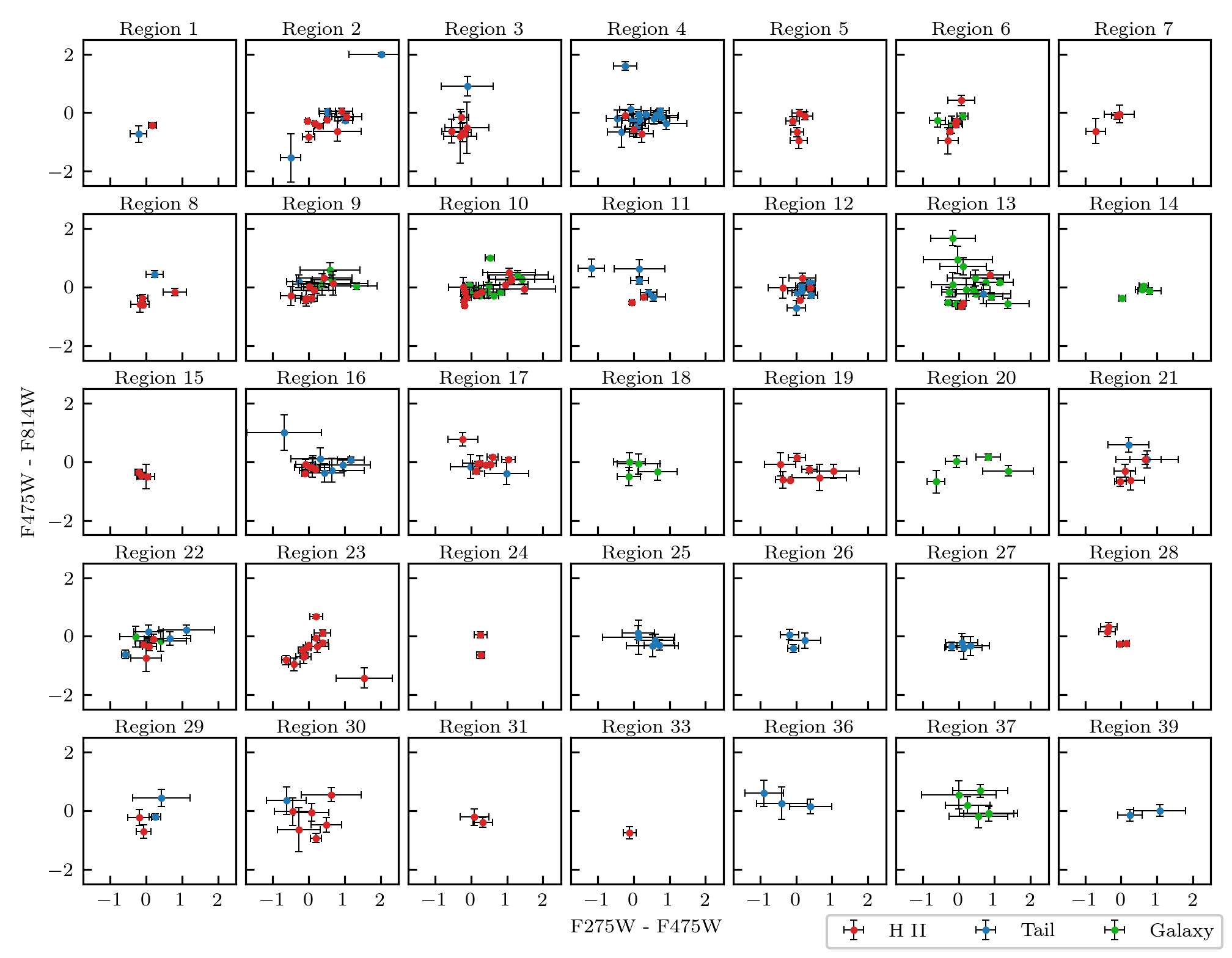
Figure 20: The colors of individual sources in the clumps defined in Fig. 1. Regions selected for CO emission but without any detected HST blue sources are not included here. One can see sources in proximity typically have similar colors.

A.3 SFR Measurement Comparison

Section 5.2 briefly notes that the HST cc/̄SFR is approximately half that of the MUSE EW SFR. Fig. A.3 shows the region-by-region SFR measurement comparison for the H ii regions discussed in Section 4.1 and Figs. 6, 8 and 10. In general, the MUSE SFR is higher than the HST cc/̄SFR. The dashed line in this figure shows unity while the dotted line shows the best fit ratio of 0.52.

References

- Astropy Collaboration et al. (2013) Astropy Collaboration et al., 2013, A&A, 558, A33
- Astropy Collaboration et al. (2018) Astropy Collaboration et al., 2018, AJ, 156, 123
- Auld et al. (2013) Auld R., et al., 2013, MNRAS, 428, 1880
- Avila et al. (2015) Avila R. J., Hack W., Cara M., Borncamp D., Mack J., Smith L., Ubeda L., 2015, in Taylor A. R., Rosolowsky E., eds, Astronomical Society of the Pacific Conference Series Vol. 495, Astronomical Data Analysis Software an Systems XXIV (ADASS XXIV). p. 281 (arXiv:1411.5605)
- Bekki & Couch (2003) Bekki K., Couch W. J., 2003, ApJ, 596, L13
- Bertin & Arnouts (1996) Bertin E., Arnouts S., 1996, A&AS, 117, 393
- Bocchio (2014) Bocchio M., 2014, PhD thesis, Institut d’Astrophysique Spatiale (IAS), UMR 8617, CNRS/Université Paris-Sud, 91405 Orsay, France
- Boselli et al. (2022) Boselli A., Fossati M., Sun M., 2022, A&ARv, 30, 3
- Calzetti (1997) Calzetti D., 1997, AJ, 113, 162
- Calzetti et al. (1994) Calzetti D., Kinney A. L., Storchi-Bergmann T., 1994, ApJ, 429, 582
- Calzetti et al. (2000) Calzetti D., Armus L., Bohlin R. C., Kinney A. L., Koornneef J., Storchi-Bergmann T., 2000, ApJ, 533, 682
- Charlot & Fall (2000) Charlot S., Fall S. M., 2000, ApJ, 539, 718
- Cramer et al. (2019) Cramer W. J., Kenney J. D. P., Sun M., Crowl H., Yagi M., Jáchym P., Roediger E., Waldron W., 2019, ApJ, 870, 63
- Davies et al. (2012) Davies J. I., et al., 2012, MNRAS, 419, 3505
- Dowell et al. (2014) Dowell C. D., et al., 2014, ApJ, 780, 75
- Dressel (2022) Dressel L., 2022, WFC3 Instrument Handbook for Cycle 30 v. 14
- Dressler (1980) Dressler A., 1980, ApJ, 236, 351
- Ekström et al. (2012) Ekström S., et al., 2012, A&A, 537, A146
- Ferland et al. (2017) Ferland G. J., et al., 2017, Rev. Mex. Astron. Astrofis., 53, 385
- Foreman-Mackey et al. (2013) Foreman-Mackey D., Hogg D. W., Lang D., Goodman J., 2013, PASP, 125, 306
- Fossati et al. (2016) Fossati M., Fumagalli M., Boselli A., Gavazzi G., Sun M., Wilman D. J., 2016, MNRAS, 455, 2028
- Fumagalli et al. (2014) Fumagalli M., Fossati M., Hau G. K. T., Gavazzi G., Bower R., Sun M., Boselli A., 2014, MNRAS, 445, 4335
- George et al. (2018) George K., et al., 2018, MNRAS, 479, 4126
- Gonzaga et al. (2012) Gonzaga S., Hack W., Fruchter A., Mack J., 2012, The DrizzlePac Handbook. STScI, Baltimore
- Gunn & Gott (1972) Gunn J. E., Gott III J. R., 1972, ApJ, 176, 1
- Hammer et al. (2010) Hammer D., et al., 2010, The Astrophysical Journal Supplement Series, 191, 143
- Hao et al. (2011) Hao C.-N., Kennicutt R. C., Johnson B. D., Calzetti D., Dale D. A., Moustakas J., 2011, ApJ, 741, 124
- Hoffmann et al. (2021) Hoffmann S. L., Mack J., Avila R., Martlin C., Cohen Y., Bajaj V., 2021, in American Astronomical Society Meeting Abstracts. p. 216.02
- Indebetouw et al. (2005) Indebetouw R., et al., 2005, ApJ, 619, 931
- Jáchym et al. (2014) Jáchym P., Combes F., Cortese L., Sun M., Kenney J. D. P., 2014, ApJ, 792, 11
- Jáchym et al. (2019) Jáchym P., et al., 2019, ApJ, 883, 145
- Kenney et al. (2015) Kenney J. D. P., Abramson A., Bravo-Alfaro H., 2015, AJ, 150, 59
- Koekemoer et al. (2003) Koekemoer A. M., Fruchter A. S., Hook R. N., Hack W., 2003, in Arribas S., Koekemoer A., Whitmore B., eds, HST Calibration Workshop : Hubble after the Installation of the ACS and the NICMOS Cooling System. p. 337
- Koyama et al. (2019) Koyama Y., Shimakawa R., Yamamura I., Kodama T., Hayashi M., 2019, PASJ, 71, 8
- Kroupa (2001) Kroupa P., 2001, MNRAS, 322, 231
- Lange et al. (2015) Lange R., et al., 2015, MNRAS, 447, 2603
- Lasker et al. (2008) Lasker B. M., et al., 2008, AJ, 136, 735
- Laudari et al. (2022) Laudari S., et al., 2022, MNRAS, 509, 3938
- Lee et al. (2013) Lee J. C., Hwang H. S., Ko J., 2013, ApJ, 774, 62
- Leitherer et al. (1999) Leitherer C., et al., 1999, ApJS, 123, 3
- Linden et al. (2021) Linden S. T., et al., 2021, ApJ, 923, 278
- Luo et al. (2022) Luo R., et al., 2022, arXiv e-prints, p. arXiv:2212.03891
- Makarov et al. (2014) Makarov D., Prugniel P., Terekhova N., Courtois H., Vauglin I., 2014, A&A, 570, A13
- Moeller & Calzetti (2022) Moeller C., Calzetti D., 2022, AJ, 163, 16
- Peng et al. (2002) Peng C. Y., Ho L. C., Impey C. D., Rix H.-W., 2002, AJ, 124, 266
- Poggianti et al. (2019) Poggianti B. M., et al., 2019, MNRAS, 482, 4466
- Poutanen et al. (2013) Poutanen J., Fabrika S., Valeev A. F., Sholukhova O., Greiner J., 2013, MNRAS, 432, 506
- Price et al. (2014) Price S. H., et al., 2014, ApJ, 788, 86
- Quilis et al. (2000) Quilis V., Moore B., Bower R., 2000, Science, 288, 1617
- Reddy et al. (2015) Reddy N. A., et al., 2015, ApJ, 806, 259
- Ryon (2022) Ryon J. E., 2022, ACS Instrument Handbook for Cycle 30 v. 21.0
- Schlafly & Finkbeiner (2011) Schlafly E. F., Finkbeiner D. P., 2011, ApJ, 737, 103
- Sivanandam et al. (2010) Sivanandam S., Rieke M. J., Rieke G. H., 2010, ApJ, 717, 147
- Sun et al. (2006) Sun M., Jones C., Forman W., Nulsen P. E. J., Donahue M., Voit G. M., 2006, ApJ, 637, L81
- Sun et al. (2007) Sun M., Donahue M., Voit G. M., 2007, ApJ, 671, 190
- Sun et al. (2010) Sun M., Donahue M., Roediger E., Nulsen P. E. J., Voit G. M., Sarazin C., Forman W., Jones C., 2010, ApJ, 708, 946
- Sun et al. (2022) Sun M., et al., 2022, Nature Astronomy, 6, 270
- Wild et al. (2011) Wild V., Charlot S., Brinchmann J., Heckman T., Vince O., Pacifici C., Chevallard J., 2011, MNRAS, 417, 1760
- Wofford et al. (2016) Wofford A., et al., 2016, MNRAS, 457, 4296
- Woudt et al. (2004) Woudt P. A., Kraan-Korteweg R. C., Cayatte V., Balkowski C., Felenbok P., 2004, A&A, 415, 9
- Wuyts et al. (2011) Wuyts S., et al., 2011, ApJ, 738, 106
- da Silva et al. (2012) da Silva R. L., Fumagalli M., Krumholz M., 2012, ApJ, 745, 145