A Lanczos approach to the Adiabatic Gauge Potential

Abstract

The Adiabatic Gauge Potential (AGP) is the generator of adiabatic deformations between quantum eigenstates. There are many ways to construct the AGP operator and evaluate the AGP norm. Recently, it was proposed that a Gram-Schmidt-type algorithm can be used to explicitly evaluate the expression of the AGP Hatomura and Takahashi (2021). We employ a version of this approach by using the Lanczos algorithm to evaluate the AGP operator in terms of Krylov vectors and the AGP norm in terms of the Lanczos coefficients. It has the advantage of minimizing redundancies in evaluating the nested commutators in the analytic expression for the AGP operator. The algorithm is used to explicitly construct the AGP operator for some simple systems. We derive an integral transform relation between the AGP norm and the autocorrelation function of the deformation operator. We present a modification of the Variational approach to derive the regulated AGP norm. Using this, we approximate the AGP to varying degrees of success. Finally, we compare and contrast the quantum-chaos-probing capacities of the AGP and K-complexity in view of the Operator Growth Hypothesis.

I Introduction

The study of quantum chaos has been the focus of a large body of research over the last century. These works have led to various insights on thermalization, information scrambling, and many other phenomena in many-body physics as well as holography. In classical physics, chaos is a well-understood phenomenon. It is usually understood in terms of classical phase space trajectories. When an infinitesimal initial perturbation in the phase space variables ends up causing an exponentially large change at late times, it is understood as (classical) chaotic dynamics. This is the well-known “butterfly effect” Roberts and Stanford (2015); Roberts and Swingle (2016).

This definition does not carry over to quantum mechanics since trajectories are no longer well-defined objects. In quantum mechanics, there is no first-principle definition of chaos yet. Instead, there are various probes of chaotic quantum dynamics. Some of the probes focus on the nature of the eigenvalues (such as spectral statistics Bohigas et al. (1984); Berry et al. (1977), eigenstate thermalization hypothesis Srednicki (1994a); Deutsch (2018); D’Alessio et al. (2016), etc.). Other probes focus on the spreading of operators within the system. These include probes such as operator size Roberts et al. (2015, 2018); Qi and Streicher (2019); Lensky et al. (2020); Schuster et al. (2022), out-of-time-ordered-correlators (OTOCs) Rozenbaum et al. (2017); Hashimoto et al. (2017); Nahum et al. (2018); Xu et al. (2020); Zhou and Swingle (2021); Gu et al. (2022) and Krylov complexity Parker et al. (2019); Barbón et al. (2019); Rabinovici et al. (2021); Bhattacharjee et al. (2022a). Part of our focus in this article will be on (the machinery of) Krylov complexity, which has found wide-ranging applications from a few body systems to quantum field theories to open quantum systems. Barbón et al. (2019); Bhattacharjee et al. (2022a); Avdoshkin and Dymarsky (2020); Dymarsky and Gorsky (2020); Jian et al. (2021); Rabinovici et al. (2021); Cao (2021); Dymarsky and Smolkin (2021); Kar et al. (2022); Caputa et al. (2022); Kim et al. (2022); Magan and Simon (2020); Caputa and Datta (2021); Bhattacharya et al. (2022); Rabinovici et al. (2022a); Mück and Yang (2022); Liu et al. (2022); Patramanis (2022); Caputa and Liu (2022); Rabinovici et al. (2022b); Fan (2022a, b); Trigueros and Lin (2022); Hörnedal et al. (2022); Balasubramanian et al. (2022a); Bhattacharjee et al. (2022b); Heveling et al. (2022); Caputa et al. (2023); Balasubramanian et al. (2022b); Afrasiar et al. (2022); Guo (2022); Bhattacharjee et al. (2022c).

Another probe that has been considered in the study of quantum chaos is the Adiabatic Gauge Potential Pandey et al. (2020) (AGP). The Adiabatic Gauge Potential (AGP) is the generator of adiabatic deformations between quantum eigenstates. In a precise sense, the distance between two eigenstates (i.e., the Fubini-Study metric Kolodrubetz et al. (2017a); Page (1987)) is the Frobenius norm of the AGP (operator) Kolodrubetz et al. (2017a); Berry (2009); Demirplak and Rice (2005, 2003); Sels and Polkovnikov (2017). It has been observed that the (regularised) AGP demonstrates different scaling behaviors (with system size) for chaotic and integrable systems. This norm scales exponentially with the system size for chaotic systems following ETH Kolodrubetz et al. (2017a). It has the potential to serve as a probe of quantum chaos. It has also been considered in the study of thermalization Nandy et al. (2022). The Adiabatic Gauge Potential itself has a rich history of being studied in various ways Jarzynski (1995); Deffner et al. (2014); Jarzynski (2013); Sierant et al. (2019); Maksymov et al. (2019); Pandey (2021). It is a unique probe since it straddles the fine line between operator dynamics and eigenstate statistics, incorporating both the information about eigenstates as well as the specific operator choice.

We study the AGP by utilizing the Lanczos algorithm Viswanath and Müller (1994a), which is a central ingredient in the formalism of Krylov complexity Parker et al. (2019). The language of the Krylov basis (generated from the Lanczos algorithm) provides a way to construct the AGP operator by evaluating the minimum number of nested commutators (of the Hamiltonian with the deforming operator). A similar prescription was proposed in Hatomura and Takahashi (2021). The prescription described there is somewhat general. In our article, we focus on the Lanczos algorithm (which is an instance of the general algorithm in Hatomura and Takahashi (2021)) and utilize it to derive an explicit expression for the AGP operators of various systems and deformations. We write the AGP operator in the Krylov language. We also study the equivalence between the variational approach towards constructing the AGP Sels and Polkovnikov (2017) and the Krylov construction. We generalize the variational approach to regularised AGP and demonstrate a method (based on this approach) to evaluate the AGP norm. We discuss how well this approach approximates the AGP for chaotic and integrable systems. Finally, we compare and contrast AGP and K-complexity as probes of chaos and phase transitions.

II Adiabatic Eigenstate Deformation

Consider a Hamiltonian $H(\lambda)$, which is a function of a tunable parameter $\lambda$. Instantaneously in $\lambda$, the eigenstates of H are defined as follows

$$H(\lambda)\ket{n(\lambda)}=E_{n}(\lambda)\ket{n(\lambda)}\,.$$ (1)

where $\ket{n(\lambda)}$ is the eigenstate with corresponding eigenvalue $E_{n}(\lambda)$. The adiabatic gauge potential, or AGP, is introduced by transforming to the moving frame of $\lambda$, characterized by the instantaneous energy basis. In this moving frame, the Hamiltonian is diagonal. This can be observed by considering the time evolution of a state $\ket{\psi}$ in the moving frame where it becomes $\ket{\tilde{\psi}}=U^{\dagger}(\lambda(t))\ket{\psi}$. Here $U$ is the unitary operator that transforms between the bases. For the sake of generality, the parameter $\lambda$ is taken to be a function of time $t$.

In the moving frame, this state evolves as

$$i\hbar\partial_{t}\ket{\tilde{\psi}}=\left(U^{\dagger}HU-i\hbar\,\dot{\lambda}\,U^{\dagger}\partial_{\lambda}U\right)\ket{\tilde{\psi}}\,.$$ (2)

The first term, $U^{\dagger}HU$, is diagonal by definition. The off-diagonal contribution comes from the second term $i\hbar\,\dot{\lambda}\,U^{\dagger}\partial_{\lambda}U$. This term is responsible for excitations between eigenstates, quantified by the velocity $\dot{\lambda}$. The AGP in the moving frame is defined as this off-diagonal term

$$\tilde{A}_{\lambda}=i\hbar\,U^{\dagger}\partial_{\lambda}U\,.$$ (3)

It is clear that if this extra term is added to the Hamiltonian $H$, then the shifted Hamiltonian $H^{\prime}$ will naturally become diagonal in the moving frame. Thus the system can demonstrate transition-less driving at arbitrary rates. Formally, we denote this as

$$H^{\prime}=H+\dot{\lambda}A_{\lambda}$$ (4)

where we have denoted the AGP in the lab frame as $A_{\lambda}=U\tilde{A}_{\lambda}U^{\dagger}=i\partial_{\lambda}$.

The object we seek to study is the AGP in the lab frame. The matrix elements of the same, in the eigenbasis of the original Hamiltonian $H(\lambda)$, can be written via the Feynmann-Hellmann theorem Feynman (1939)

$$\bra{m}A_{\lambda}\ket{n}=-i\frac{\bra{m}\partial_{\lambda}H\ket{n}}{E_{m}-E_{n}}\;\;\;\forall\;\;m\neq n\,.$$ (5)

An equivalent expression for the AGP can be obtained from the commutator equation $[H,i\partial_{\lambda}H+[H,A_{\lambda}]]=0$ Kolodrubetz et al. (2017b); Jarzynski (2013). It is worth noting that the AGP has inherent gauge freedom associated with the choice of the phase of the eigenstates of $H$. In the matrix form, this translates into the freedom to choose the diagonal elements of the AGP. In the operator picture, the gauge freedom is realized by adding any operator $K$ to the AGP such that $[H,K]=0$ (i.e., shifting by any conserved charge in the theory).

The regularized AGP Pandey et al. (2020) is defined in terms of the operator $A_{\lambda}$ by taking the expectation value of the same between the eigenstates of the Hamiltonian $H(\lambda)$ and taking the square of the magnitude of the same. Finally, the eigenstates are summed over. In other words, it is written as

$$||A_{\lambda}||^{2} =\frac{1}{\mathcal{D}}\sum_{m\neq n}|\bra{m}A_{\lambda}\ket{n}|^{2}$$

$$=\frac{1}{\mathcal{D}}\sum_{m\neq n}\frac{\omega^{2}_{mn}}{(\mu^{2}+\omega^{2}_{mn})^{2}}|\bra{m}\partial_{\lambda}H\ket{n}|^{2}\,.$$ (6)

where $\mathcal{D}$ is the dimension of the Hilbert space and $\omega_{mn}=E_{m}-E_{n}$, i.e. the difference between eigenvalues.

III Lanczos Algorithm and Krylov complexity

The notion of Krylov complexity involves choosing an appropriate basis (in the Hilbert space of operators or states) to describe the time evolution of an operator. While there can exist infinite possible such bases, there is a unique choice that corresponds to the minimal basis with respect to some appropriately defined cost functional. We only discuss operator complexity in this paper. For state complexity and its applications, the reader is directed to Parker et al. (2019); Balasubramanian et al. (2022a); Bhattacharjee et al. (2022b); Afrasiar et al. (2022).

Arriving at the appropriate basis (known as Krylov basis) involves writing the time-evolved operator $\mathcal{O}(t)$ in terms of nested commutators. This follows from the Baker-Campbell-Hausdorff formula

$$\mathcal{O}(t) =e^{iHt/\hbar}\mathcal{O}e^{-iHt/\hbar}$$

$$=\mathcal{O}+\frac{it}{\hbar}[H,\mathcal{O}]+\frac{(it)^{2}}{2!\,\hbar^{2}}[H,[H,\mathcal{O}]]$$

$$+\frac{(it)^{3}}{3!\,\hbar^{3}}[H,[H,[H,\mathcal{O}]]]+\frac{(it)^{4}}{4!\,\hbar^{4}}[H,[H,[H,[H,\mathcal{O}]]]]$$

$$+\cdots\leavevmode\nobreak\ \leavevmode\nobreak\ .$$ (7)

Each term in the BCH expansion is then chosen as the basis elements of our initial basis $\mathfrak{D}$. The elements of the basis are then written as

$$\mathfrak{D}=\{\mathcal{O},[H,\mathcal{O}],[H,[H,\mathcal{O}]],[H,[H,[H,\mathcal{O}]]],\cdots\}$$ (8)

This basis is conveniently represented in the language of the Louivillian super-operator $\mathcal{L}$, which is defined as

$$\mathcal{L}(\ast)=[H,\ast]$$ (9)

which allows us to write the basis $\mathfrak{D}$ as

$$\mathfrak{D}=\text{span}\{\mathcal{L}^{n}\mathcal{O}\}_{n=0}^{+\infty}$$ (10)

The algorithm for generating the Krylov basis from $\mathfrak{D}$ is known as the Lanczos algorithm Viswanath and Müller (1994a). It is a Gram-Schmidt-like recursive orthonormalization protocol. We start with the normalized initial operator $\mathcal{O}_{0}$. Normalization is defined via the Wightman inner product (at inverse temperature $\beta=0$), written as $(\mathcal{O}|\mathcal{O}^{\prime})=\frac{1}{\mathcal{N}}\mathrm{Tr}(\mathcal{O}^{\dagger}\mathcal{O}^{\prime})$, where $\mathcal{N}=\text{Tr}(\mathbf{1})$ is the dimension of the Hilbert space of operators.

The algorithm proceeds as follows.

• Start with the definition $A_{0}\equiv\mathcal{O}_{0}$, which we assume to be normalized $(\mathcal{O}_{0}|\mathcal{O}_{0})=1$. This is the $0^{\text{th}}$ Krylov vector.

• Define $A_{1}=\mathcal{L}\mathcal{O}_{0}$, and normalize it with $b_{1}=\sqrt{(A_{1}|A_{1})}$. Define the normalized operator $\mathcal{O}_{1}=b_{1}^{-1}A_{1}$. This is the $1^{\text{st}}$ Krylov vector.

• From this, given $\mathcal{O}_{n-1}$ and $\mathcal{O}_{n-2}$, we can construct the following operators

  $$A_{n}=\mathcal{L}\mathcal{O}_{n-1}-b_{n-1}\mathcal{O}_{n-2}\,.$$ (11)

  This can be normalized as $b_{n}=\sqrt{(A_{n}|A_{n})}$ and the $n^{\mathrm{th}}$ Krylov vector is given by $\mathcal{O}_{n}=b_{n}^{-1}A_{n}$.

• Terminate the algorithm when $b_{n}$ hits zero.

The features of this Krylov space formed by $\text{span}\{\mathcal{O}_{n}\}$ are extensive and cannot fit into this tiny section. We refer the readers to Rabinovici et al. (2022b, 2021, a); Barbón et al. (2019) for an exhaustive review. For our purposes, it will suffice to know that the dimensions of the Krylov subspace thus formed is given by $K\leq\mathcal{D}^{2}-\mathcal{D}+1$, where $\mathcal{D}$ is the dimension of the Hilbert space generated by the Hamiltonian $H$. This also implies that the span in (10) is up to $n=K$ in reality.

The time evolved operator $\mathcal{O}(t)$ is then written in terms of the Krylov basis operators $\mathcal{O}_{n}$ as

$$\mathcal{O}(t)=\sum_{n=0}^{K}i^{n}\psi_{n}(t)\mathcal{O}_{n}\,.$$ (12)

The time-dependent coefficients thus obtained $\psi_{n}(t)$ are known as the Krylov basis wavefunctions and contain the time evolution information. These wavefunctions satisfy the following recursive “Schrödinger equation”, which can be seen from the Lanczos algorithm

$$\partial_{t}\psi_{n}(t)=-b_{n+1}\psi_{n+1}(t)+b_{n}\psi_{n-1}(t)\,.$$ (13)

where $\psi_{n}(0)=\delta_{n0}$ and $b_{0}=\psi_{-1}=0$.

We focus only on Hermitian initial operators $\mathcal{O}^{\dagger}_{0}=\mathcal{O}_{0}$. The mechanism of the Krylov construction is ill-understood for non-Hermitian operators. A few facts for Hermitian $\mathcal{O}_{0}$ follow from the Lanczos algorithm. Firstly, one can note that $\mathcal{O}_{2n}$ are Hermitian for all $n$ and $\mathcal{O}_{2n+1}$ are anti-Hermitian. This is the motivation behind the $i^{n}$ in the expression (12), which ensures that $\psi_{n}(t)$ are real functions.

Secondly, one can note that for Hermitian initial operator $\mathcal{O}_{0}$, the Louivillian super-operator can be realized in the following matrix form

$$L_{mn}=(\mathcal{O}_{m}|\mathcal{L}|\mathcal{O}_{n})=\begin{pmatrix}0&b_{1}&0&0&\cdots\\ b_{1}&0&b_{2}&0&\cdots\\ 0&b_{2}&0&b_{3}&\cdots\\ 0&0&b_{3}&0&\cdots\\ \vdots&\vdots&\vdots&\vdots&\ddots\end{pmatrix}$$ (14)

where the matrix element $(\mathcal{O}_{m}|\mathcal{L}|\mathcal{O}_{n})$ is given by the inner product $\frac{1}{\mathcal{N}}\text{Tr}(\mathcal{O}^{\dagger}_{m}\mathcal{L}\mathcal{O}_{n})$.

The machinery of Krylov complexity with the Lanczos coefficients $b_{n}$, the wavefunctions $\psi_{n}(t)$ and the basis operators $\mathcal{O}_{n}$ together provide a complete set of tools to describe the nature of time evolution of the Hermitian operator $\mathcal{O}(t)$. We defer the description of the actual quantity known as Krylov complexity to the next section.

III.1 Universal Operator Growth Hypothesis

In this section, we will discuss a proposal for using the technology described above to probe chaotic dynamics. The proposal Parker et al. (2019) is known as the “Universal Operator Growth Hypothesis”. The fundamental claim is that for chaotic systems, the Lanczos coefficients $b_{n}$ show asymptotically linear growth with $n$. For other systems, the growth is sublinear. In other words, the maximum possible growth of the Lanczos coefficients (under some assumptions) is linear in $n$. The Krylov complexity is defined as

$$K(t)=(\mathcal{O}(t)|n|\mathcal{O}(t))=\sum_{n=0}^{K}n|\phi_{n}(t)|^{2}\,.$$ (15)

shown an exponential growth $K(t)\sim e^{2\alpha t}$ for chaotic systems. The coefficient $\alpha$ is system dependent and corresponds to the slope of linear growth of $b_{n}$ (i.e., $b_{n}\sim\alpha n$). It also serves as an upper bound to the Lyapunov constant $\lambda\leq 2\alpha$.

Intricately related to K-complexity, there are a few other quantities that embody the operator growth hypothesis equally well. These quantities contain exactly the same amount of information as K-complexity and the Lanczos coefficients do. These are the autocorrelation function.

$$\mathcal{C}(t)=(\mathcal{O}(t)|\mathcal{O})=\frac{\text{Tr}(\mathcal{O}^{\dagger}(t)\mathcal{O})}{\text{Tr}(\mathbf{1})}=(\mathcal{O}|e^{i\mathcal{L}t}|\mathcal{O})\,.$$ (16)

The autocorrelation function has the following Taylor series expansion in $t$

$$\mathcal{C}(-it)=\sum_{n}\frac{m_{2n}}{(2n)!}t^{2n}$$ (17)

An equivalent statement of the Operator Growth Hypothesis for chaotic systems is that the moments $m_{2n}$ go as $n^{2n}e^{O(n)}$ asymptotically. The Lanczos coefficients can be obtained from the moments via a recursive algorithm Viswanath and Müller (1994a).

Certain transforms of the autocorrelation function are also of interest. These are the spectral function $\Phi(\omega)$ and the Green’s function $G(z)$ defined as

$$\Phi(\omega) =\int_{-\infty}^{\infty}\mathcal{C}(t)e^{i\omega t}\mathrm{d}t\,.$$ (18)

$$G(z) =(\mathcal{O}|\frac{1}{z-\mathcal{L}}|\mathcal{O})=i\int_{0}^{\infty}e^{-izt}\mathcal{C}(t)\mathrm{d}t\,.$$ (19)

Finally, the exponential growth of Krylov complexity(i.e., chaotic systems) corresponds to the presence of a series of complex poles for the autocorrelation function, with the pole closest to the real axis given by $t=\frac{\pm i\pi}{2\alpha}$. Additionally, it also implies a large-$\omega$ fall-off for $\Phi(\omega)$, of the form $e^{-\omega\pi/2\alpha}$. This behavior is also consistent with ETH, as we shall see.

IV The Formalism

In this section, we will consider the Regularized Adiabatic Gauge Potential Pandey et al. (2020) in the Krylov/Lanczos language. The regularized AGP operator, in a particular choice of gauge (where its’ diagonal elements are $0$), is given by the following expression (for the Hamiltonian $H(\lambda)$)

$$A_{\lambda}=-\frac{1}{2}\int_{-\infty}^{\infty}\text{sgn}(t)e^{-\mu|t|}\left(\partial_{\lambda}H\right)(t)\mathrm{d}t\,.$$ (20)

Here $\mu$ is an infinitesimal regulator. When evaluating the AGP norm to study chaotic and integrable dynamics, it is convenient to choose $\mu=L2^{-L}$ where $L$ is the system size. Unless otherwise mentioned, the operators and eigenstates are to be taken as functions of the adiabatic parameter $\lambda$.

The machinery of Krylov complexity serves as a natural approach to characterizing the $\partial_{\lambda}H(t)$ term, provided this term is Hermitian. For the rest of this work, we shall assume that this term is normalized appropriately by the trace norm $(A|B)$ at $t=0$. One can regain the results for the unnormalized AGP operator by multiplying the final result by its trace norm $||\partial_{\lambda}H||$.

Using (12) the operator $A_{\lambda}$ can be written as

$$A_{\lambda}=-\frac{1}{2}\int_{-\infty}^{\infty}\text{sgn}(t)e^{-\mu|t|}\sum_{n=0}^{K}i^{n}\psi_{n}(t)\mathcal{O}_{n}\mathrm{d}t\,.$$ (21)

The knowledge of the Krylov basis vectors and the Krylov wavefunctions is enough to construct the AGP. The Lanczos algorithm minimizes the number of terms (i.e., nested commutators) that need to be calculated (analytically) when evaluating $\mathcal{O}(t)$. Therefore, in that respect, this process achieves the evaluation of $A_{\lambda}$ with the minimum number of analytic evaluations.

The only contribution in (21) is from the odd indexed Krylov vectors, i.e., only from operators of the form $\mathcal{O}_{2k+1}$. This is due to the fact that $\psi_{n}(-t)=(-1)^{n}\psi_{n}(t)$. Therefore (21) reduces to

$$A_{\lambda}=-\sum_{n=0}^{M}\alpha_{2n+1}\mathcal{O}_{2n+1}\,.$$ (22)

where

$$\alpha_{2n+1}=\int_{0}^{\infty}i^{2n+1}e^{-\mu t}\psi_{2n+1}(t)\mathrm{d}t\,.$$ (23)

and $M=\frac{K-1}{2}$ if $K$ is odd or $M=\frac{K}{2}-1$ if $K$ is even. Using this, the AGP norm can be written as (detailed derivation in Appendix A)

$$||A_{\lambda}||^{2}=-\sum_{n=0}^{M}\alpha_{2n+1}^{2}$$ (24)

This construction provides an alternate representation of the AGP operator. A nice consistency check of this expression is to check the gauge choice of $A_{\lambda}$. The gauge choice in this section corresponds to the diagonal elements of $A_{\lambda}$ being set to $0$. This is reflected via the fact that $\bra{n}\mathcal{O}_{2n+1}\ket{n}=0\;\;\forall\;n$. This follows from the Lanczos algorithm (described in the previous section) and the fact that $\bra{n}[H,Q]\ket{n}=0$ for any operator $Q$ and eigenstate $\ket{n}$ of the hermitian Hamiltonian $H$.

IV.1 The response function

The response function(as defined in Pandey et al. (2020)) provides another representation of the AGP norm. It is interesting since it possesses a direct interpretation within the ETH ansatz Srednicki (1994b). The response function is defined as

$$\overline{|f_{\lambda}(\omega)|}^{2} =\frac{1}{\mathcal{D}}\sum_{n}\sum_{n\neq m}|\bra{m}\partial_{\lambda}H\ket{n}|^{2}\delta(\omega_{mn}-\omega)$$

$$=\frac{1}{\mathcal{D}}\sum_{n}\int_{-\infty}^{\infty}\frac{\mathrm{d}t}{4\pi}e^{i\omega t}\bra{n}\{\partial_{\lambda}H(t),\partial_{\lambda}H\}\ket{n}_{c}$$ (25)

where the connected component of the expectation value is defined as $\bra{n}AB\ket{n}_{c}=\bra{n}AB\ket{n}-\bra{n}A\ket{n}\bra{n}B\ket{n}$. The sum is over the instantaneous eigenstates of $H$. This expression reduces to

$$\overline{|f_{\lambda}(\omega)|}^{2}=\frac{1}{\mathcal{D}} \sum_{n}\int_{-\infty}^{\infty}\frac{\mathrm{d}t}{2\pi}e^{i\omega t}\Big{(}\bra{n}\partial_{\lambda}H(t)\partial_{\lambda}H(0)\ket{n}$$

$$-\bra{n}\partial_{\lambda}H(t)\ket{n}\bra{n}\partial_{\lambda}H(0)\ket{n}\Big{)}\,.$$ (26)

Using (16) and $\bra{n}\partial_{\lambda}H(t)\ket{n}=\bra{n}\partial_{\lambda}H(0)\ket{n}$, we obtain the following expression

$$\overline{|f_{\lambda}(\omega)|}^{2}=\int_{-\infty}^{\infty}\frac{\mathrm{d}t}{2\pi}e^{i\omega t}\mathcal{C}(t)-\frac{1}{\mathcal{D}}\sum_{n}\bra{n}\partial_{\lambda}H(0)\ket{n}^{2}\delta(\omega)\,.$$ (27)

The response function $\overline{|f_{\lambda}(\omega)|}^{2}$ is nearly the same as the spectral function defined in (18). We denote the extra term (proportional to $\delta(\omega)$) by $\varPhi_{0}$. The response function is written as

$$\overline{|f_{\lambda}(\omega)|}^{2}=\Phi(\omega)-\varPhi_{0}\delta(\omega)$$ (28)

For large $\omega$, the only contribution comes from $\Phi(\omega)$. It was demonstrated in LeBlond et al. (2019); Brenes et al. (2020a, b) that the averaged over eigenstates squared of the ETH spectral function $f_{\lambda}(\omega)$ decays as $\sim e^{-\omega^{n}},\,n>1$ for integrable systems and as $\sim e^{-\omega}$ for chaotic systems. This behavior is straightforward to note from the properties of the function $\Phi(\omega)$.

It is known Parker et al. (2019); Viswanath and Müller (1994b) that the decay rate of the spectral function $\Phi(\omega)$ is bounded above by $e^{-k|\omega|}$. The exact decay rate goes as $\sim e^{-|\omega/\omega_{0}|^{1/\delta}}$ (where $\omega_{0}=\frac{2}{\pi}\alpha$). The Lanczos coefficients for the same system grow (asymptotically) as $b_{n}\sim n^{\delta}$ (where $\delta\leq 1$). Therefore, for integrable systems (as identified in terms of the Operator Growth Hypothesis), it is expected that the spectral function, and by extension the response function, will decay faster than $\sim e^{-\omega}$ for large $\omega$. For chaotic systems (again, in the Operator Growth Hypothesis definition), it is expected that the spectral function (and thus the response function) will decay as $\sim e^{-\omega}$. These results follow from the statement of the Operator Growth Hypothesis, which states that chaotic systems exhibit linear growth of Lanczos coefficients (i.e., $\delta=1$) and non-chaotic systems exhibit sublinear growth (i.e., $\delta<1$). Therefore, we find evidence that within the ETH regime, the Operator Growth Hypothesis is compatible with ETH.

Returning to the regularized AGP norm, with a bit of algebra, one can show that

$$||A_{\lambda}||^{2}=\frac{1}{2}\int_{0}^{\infty}\mathrm{d}t\left(\frac{1}{\mu}-t\right)\mathcal{C}(t)e^{-\mu t}\,.$$ (29)

The regularized AGP norm can also be expressed in terms of the Krylov Greens’ function

$$||A_{\lambda}||^{2}=-\frac{i}{2}\left(\frac{1}{\mu}+\partial_{\mu}\right)G(i\mu)\,.$$ (30)

It is also possible to describe the AGP norm solely in terms of the Lanczos coefficients. The formal expression is discussed in Appendix A. In the next section, we introduce a matrix equation based on the gauge constraint Sels and Polkovnikov (2017), which allows us to evaluate the regularized AGP norm solely in terms of the Lanczos coefficient.

V A Matrix Equation

We shall now consider the gauge condition that has to be satisfied by the AGP operator Sels and Polkovnikov (2017); Kolodrubetz et al. (2017b)

$$[H,i\partial_{\lambda}H+[H,A_{\lambda}]]=0\,.$$ (31)

This gauge condition does not hold exactly for the regularized AGP operator. When the regulator is added to the AGP operator, it may be expressed as (20). It can be seen that the regularization implies that gauge constraint is modified to

$$[H,i\partial_{\lambda}H+[H,[H,A_{\lambda}]]+\mu^{2}A_{\lambda}=0$$ (32)

This expression is derived in Appendix C. We consider the implication of this identity vis-à-vis (22). We denote this expression as

$$A_{\lambda}=\sum_{n=0}^{M}\alpha_{2n+1}\mathcal{O}_{2n+1}$$ (33)

where $\alpha_{k}=-i^{k}\int_{0}^{\infty}e^{-\mu t}\psi_{k}(t)\mathrm{d}t$.

From the recursion relation (13), the relation for $\alpha_{n}$ follows

$$i\mu\alpha_{n}+b_{n}\alpha_{n-1}+b_{n+1}\alpha_{n+1}+i\delta_{n,0}=0\,.$$ (34)

Using this, one can demonstrate that the gauge condition (32) is satisfied.

The expression of the AGP norm (24) can be equivalently written as

$$||A_{\lambda}||^{2}=-\frac{ib_{1}}{2\mu}\partial_{\mu}\alpha_{1}$$ (35)

This expression is simply a repackaging of (30).

V.1 A set of linear equations

The constraint (32) is useful to determine the coefficients $\alpha_{2n+1}$. Computationally, it is somewhat straightforward to evaluate the Krylov vectors $\mathcal{O}_{2n+1}$ and Lanczos coefficients $b_{n}$. On the other hand, evaluating the wavefunctions $\psi_{2n+1}$ (and consequently $\alpha_{2n+1}$) becomes a very tedious process after a few wavefunctions. To circumvent this problem, one can instead solve a set of $M+1$ linear equations to determine the $M+1$ coefficients $\alpha_{2n+1}$.

Inserting the expression (33) into the gauge constraint (32) (but now leaving $\alpha_{2n+1}$ as undetermined coefficients), we obtain the following $2$ relations

$$ib_{1}+\alpha_{1}(b_{1}^{2}+b_{2}^{2}+\mu^{2})+\alpha_{3}b_{3}b_{2}=0$$ (36)

$$\alpha_{2L-1}b_{2L}b_{2L+1}+\alpha_{2L+1}(b_{2L+1}^{2}+b_{2L+2}^{2}+\mu^{2})=0$$ (37)

And the following set of $M-1$ relations

$$\alpha_{2k-1} b_{2k}b_{2k+1}+\alpha_{2k+1}(b^{2}_{2k+2}+b_{2k+1}^{2}+\mu^{2})$$

$$+ \alpha_{2k+3}b_{2k+3}b_{2k+2}=0\;\;\forall k\in\{1,M-1\}$$ (38)

This set of equations can be written in the matrix form as follows

$$\begin{bmatrix}b_{1}^{2}+b_{2}^{2}+\mu^{2}&b_{2}b_{3}&0&0&\cdots&0\\ b_{2}b_{3}&b_{3}^{2}+b_{4}^{2}+\mu^{2}&b_{4}b_{5}&0&\cdots&0\\ 0&b_{4}b_{5}&b_{5}^{2}+b_{6}^{2}+\mu^{2}&b_{6}b_{7}&\cdots&0\\ \vdots&\vdots&\vdots&\vdots&\ddots&\vdots\\ 0&0&0&\cdots&b_{2L}b_{2L+1}&b_{2L+1}^{2}+b_{2L+2}^{2}+\mu^{2}\end{bmatrix}\begin{bmatrix}\alpha_{1}\\ \alpha_{3}\\ \alpha_{5}\\ \vdots\\ \alpha_{2L+1}\end{bmatrix}=\begin{bmatrix}-ib_{1}\\ 0\\ 0\\ \vdots\\ 0\end{bmatrix}$$ (39)

Once the Lanczos coefficients $b_{n}$ have been evaluated numerically by implementing the Lanczos algorithm, the coefficients of $\mathcal{O}_{2n+1}$ can be determined by solving the matrix equation given above.

VI Analytical Examples

In this section, we evaluate some explicit expressions for the AGP using the expression (29). The full steps of the evaluation are covered in Appendix B. In the models, we require analytic expressions of the autocorrelation function. So we are naturally restricted to small integrable systems. In Appendix D, we derive an approximate analytical expression for the AGP norm of the Ising chain at criticality.

VI.1 A $2$-level system

We consider the following model del Campo et al. (2012) (demonstrating the Landau-Zener transition Zener (1932)), which is also the simplest model supporting the Kibble-Zurek mechanism Kibble (1976, 1980); Zurek (1996). This model is described by the simple Hamiltonian

$$H(\lambda)=\lambda\sigma^{z}+\Delta\sigma^{x}\,.$$ (40)

The autocorrelation function for this system can be easily evaluated, say for the operator $\sigma^{z}$

$$\mathcal{C}(t) =\frac{\text{Tr}(e^{iHt}\sigma^{z}e^{-iHt}\sigma^{z})}{\text{Tr}(\mathbf{1}_{2\times 2})}$$

$$=\frac{\left(\lambda^{2}+\Delta^{2}\cos\left(2t\sqrt{\Delta^{2}+\lambda^{2}}\right)\right)}{(\Delta^{2}+\lambda^{2})}\,.$$ (41)

Inserting this expression in (29), we obtain the following expression

$$||A_{\lambda}||^{2}=\frac{4\Delta^{2}}{\left(4\left(\Delta^{2}+\lambda^{2}\right)+\mu^{2}\right)^{2}}\xrightarrow[\mu\rightarrow 0]{}\frac{\Delta^{2}}{4(\Delta^{2}+\lambda^{2})^{2}}$$ (42)

For this system, we can take the limit $\mu\rightarrow 0$ without any issues because it does not exhibit any degeneracies. We compare this result with the AGP operator derived in del Campo et al. (2012). Using the Krylov approach, one can use (22) to derive the AGP operator. This calculation is described in detail in Appendix B. The operator thus obtained is written below.

$$A_{\lambda}=-\frac{1}{2}\frac{\Delta}{\Delta^{2}+\lambda^{2}}\sigma^{y}$$ (43)

The norm calculated from this AGP operator, using (81), can be shown to be

$$||A_{\lambda}||^{2} =\frac{1}{\mathcal{D}}\sum_{m\neq n}|\bra{m}A_{\lambda}\ket{n}|^{2}$$

$$=\frac{\Delta^{2}}{4(\Delta^{2}+\lambda^{2})^{2}}$$ (44)

which is the result obtained in (42), happily.

VI.2 A 2-qubit system

We consider the following simple $2$-qubit system Petiziol et al. (2018) given by the Hamiltonian

$$H(\lambda)=-\left(\sigma^{1}_{x}\sigma^{2}_{x}+\sigma^{1}_{z}\sigma^{2}_{z}\right)-\varepsilon(1-\lambda)\left(\sigma^{1}_{z}+\sigma^{2}_{z}\right)\,.$$ (45)

Evaluating the autocorrelation function $\mathcal{C}(t)$ (starting with $\mathcal{O}_{0}=\frac{1}{\sqrt{2}}(\sigma^{1}_{z}+\sigma^{2}_{z})$) is straightforward and gives the following result

$$\mathcal{C}(t) =\frac{\text{Tr}(e^{iHt}\mathcal{O}_{0}e^{-iHt}\mathcal{O}_{0})}{\text{Tr}(\mathbf{I}_{2\times 2})}$$

$$=\frac{4\varepsilon^{2}(1-\lambda)^{2}+\cos(2t\sqrt{1+4\varepsilon^{2}(1-\lambda)^{2}})}{1+4\varepsilon^{2}(1-\lambda)^{2}}\,.$$ (46)

From this expression, we evaluate the AGP norm using (29)

$$||A_{\lambda}||^{2}=\frac{8}{\left(16\varepsilon^{2}(1-\lambda)^{2}+4\right)^{2}}\,.$$ (47)

Note that this Hamiltonian (45) is non-degenerate for real $\varepsilon,\lambda$. Therefore, it is possible to take the limit $\mu\rightarrow 0$ in the AGP norm and operator without causing a divergence.

We employ the Lanczos algorithm in order to derive the form of the AGP operator, using (22). The result is (derivation in Appendix B)

$$A_{\lambda}=-i\frac{\sqrt{2}}{4(1+4\varepsilon^{2}(1-\lambda)^{2}}\left(\sigma^{1}_{x}\sigma^{2}_{y}+\sigma^{1}_{y}\sigma^{2}_{x}\right)\,.$$ (48)

This is not the result discussed in Petiziol et al. (2018). This is because in Petiziol et al. (2018), the AGP operator is derived with respect to the unnormalized $\partial_{\lambda}H$. The normalization factor $\sqrt{2}\varepsilon$ can be reinserted into the AGP operator to obtain the result in Petiziol et al. (2018). This implies multiplying the AGP norm (47) by $2\varepsilon^{2}$.

VI.3 A 4-body system

In this section, we consider a simple $4$-body system described by the Hamiltonian

$$H=\sum_{i=0}^{3}\sigma^{x}_{i}\sigma^{x}_{i+1}+\lambda(\sigma^{z}_{1}+\sigma^{z}_{2})\,.$$ (49)

The Krylov basis operators and the Lanczos coefficients are given in Appendix B. The initial operator is chosen as $\partial_{\lambda}H=\sigma^{z}_{1}+\sigma^{z}_{2}$. The regulator is taken to be $\mu=L2^{-L}$, with the system size $L=4$ in this case. We evaluate the AGP operator

$$A_{\lambda} =c_{1}(\sigma^{z}_{1}+\sigma^{z}_{2})+c_{2}\left(\sigma^{x}_{0}\sigma^{y}_{1}+\sigma^{y}_{2}\sigma^{x}_{3}\right)$$

$$+c_{3}\left(\sigma^{x}_{1}\sigma^{y}_{2}+\sigma^{y}_{1}\sigma^{x}_{2}\right)+c_{4}\left(\sigma^{x}_{0}\sigma^{z}_{1}\sigma^{y}_{2}+\sigma^{y}_{1}\sigma^{z}_{2}\sigma^{x}_{3}\right)$$ (50)

where

$$c_{1} =-\frac{i\left(\frac{3\sqrt{2}\lambda\left(9\lambda^{6}-184\lambda^{4}+512\lambda^{2}+1024\right)\left(\lambda^{2}\left(9\mu^{2}+272\right)+36\lambda^{4}+32\mu^{2}\right)}{\left(5\lambda^{2}+4\right)\left(9\lambda^{2}+32\right)\left|16-9\lambda^{2}\right|}+2\left(8\left(\lambda^{2}+2\right)\mu^{2}+\frac{16\lambda^{2}\left(9\lambda^{4}+50\lambda^{2}+256\right)}{9\lambda^{2}+32}+\mu^{4}\right)\right)}{8\left(3\lambda^{2}+4\right)\mu^{4}+16\left(3\lambda^{2}+4\right)^{2}\mu^{2}+64\lambda^{2}\left(4\lambda^{4}+13\lambda^{2}+32\right)+\mu^{6}}$$ (51)

$$c_{2} =-\frac{12\sqrt{2}\lambda^{2}\left(\lambda^{2}\left(5\mu^{2}+32\right)+2\lambda^{4}+4\left(\mu^{2}+16\right)\right)}{\left(5\lambda^{2}+4\right)\left(8\left(3\lambda^{2}+4\right)\mu^{4}+16\left(3\lambda^{2}+4\right)^{2}\mu^{2}+64\lambda^{2}\left(4\lambda^{4}+13\lambda^{2}+32\right)+\mu^{6}\right)}$$ (52)

$$c_{3} =\frac{8\sqrt{2}\lambda^{2}\left(27\lambda^{4}+16\lambda^{2}-64\right)}{\left(5\lambda^{2}+4\right)\left(8\left(3\lambda^{2}+4\right)\mu^{4}+16\left(3\lambda^{2}+4\right)^{2}\mu^{2}+64\lambda^{2}\left(4\lambda^{4}+13\lambda^{2}+32\right)+\mu^{6}\right)}$$ (53)

$$c_{4} =-\frac{16\sqrt{2}\lambda\left(7\lambda^{2}+\mu^{2}\right)}{8\left(3\lambda^{2}+4\right)\mu^{4}+16\left(3\lambda^{2}+4\right)^{2}\mu^{2}+64\lambda^{2}\left(4\lambda^{4}+13\lambda^{2}+32\right)+\mu^{6}}$$ (54)

The AGP norm evaluated from the expression (50) is plotted in Fig. 1 and compared with the numerically evaluated AGP norm directly from the Hamiltonian (49).

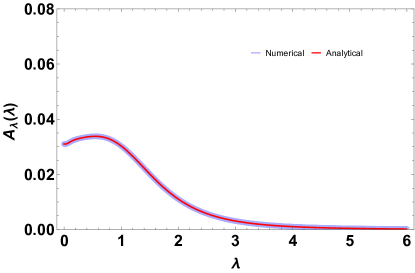
Figure 1: The AGP norm computed numerically for the Hamiltonian (49) and compared with the norm of the analytical expression (50). It is clear that the expression exactly captures the AGP, as per expectations.

VII Approximating the AGP

We have described a systematic procedure to evaluate the AGP operator. However, evaluating the full Krylov basis and all the Lanczos coefficients analytically is a painful process. Even numerically, evaluating the full AGP can prove to be non-trivial via the Lanczos approach, especially if there exists an exponentially large Krylov basis implying an exponentially large number of equations (38) that need to be solved to evaluate the AGP norm. Therefore, it is not desirable to solve the full set of equations in (38) in order to determine the AGP.

In view of the difficulty in evaluating the full Krylov basis, we consider approximating the AGP by truncating the series at (22) at some $N<M$. We terminate the series at $n=N<M$ and proceed to solve (38) with a reduced set of equations. Consequently, the dimensions of the matrix (39) will be lesser and therefore easier to solve the matrix equation for the reduced vector $\{\alpha_{1},\alpha_{2},\alpha_{3},\dots,\alpha_{2N+1}\}$. The expression for the AGP operator is then given as

$$A_{\lambda}=\sum_{n=0}^{N<M}\alpha_{2n+1}\mathcal{O}_{2n+1}$$ (55)

It is easier to evaluate the initial few Krylov vectors as compared to the ones at higher index values analytically. An explicit form of the AGP operator can be approximated by considering a small value of $N$. The expression obtained for the AGP norm $||A_{\lambda}||^{2}=-\sum_{n=0}^{N<M}\alpha_{2n+1}^{2}$ using the truncated series can be compared with the exact numerical result to determine the number of terms that need to be included to get a reasonably approximate AGP operator.

VII.1 The Variational Approach

In Sels and Polkovnikov (2017), a variational approach for evaluating the AGP operator was proposed. We now discuss the effect of truncation with respect to this approach. A similar discussion, with close results, can be found in Hatomura and Takahashi (2021). For the regulated AGP, the variational approach involves minimizing the action, defined as

$$S=\text{Tr}(G_{\lambda}^{2})=\text{Tr}((i\partial_{\lambda}H+[H,A_{\lambda}])^{2}+\mu^{2}A_{\lambda}^{2})$$ (56)

with respect to an appropriately chosen set of free parameters in the AGP operator $A_{\lambda}$. The approximate AGP operator is found by solving for the following Euler-Lagrange equation

$$\frac{\delta S(A_{\lambda})}{\delta A_{\lambda}}=0$$ (57)

We observe that choosing the $A_{\lambda}$ to be given by the expression (55) gives us the following expression for the action

$$S =(i+\alpha_{1}b_{1})^{2}+\sum_{k=1}^{N}(\alpha_{2k-1}b_{2k}+\alpha_{2k+1}b_{2k+1})^{2}$$

$$+\alpha_{2N+1}^{2}b_{2N+2}^{2}+\mu^{2}\sum_{k=0}^{N}\alpha_{2k+1}$$ (58)

It is straightforward to see that extremizing the action $S$ with respect to the free parameters $\alpha_{2k+1}$ gives back the equations (36)-(38), with $N$ instead of $L$. This is expected since any additional Krylov basis operators (added to $A_{\lambda}$) are orthonormal to the terms already included. Therefore, there is no “weight adjustment” effect (or a kind of “back-reaction”) on the coefficients equations determining the coefficients $\alpha_{2k+1}$. It is important to note that adding more terms does affect the explicit expressions of the $\alpha_{2k+1}$ (in terms of the Lanczos coefficients) already determined as they are solutions of a coupled set of linear equations.

VIII Numerical Results

We study this truncation process in three types of systems: integrable, weakly chaotic, and strongly chaotic. We find that due to the successively (nearly exponentially) increasing Krylov space dimensions for these systems, the truncation method shows decreasing levels of success in capturing the basic features of the AGP.

VIII.1 Integrable Free System

We consider the integrable (non-interacting) Ising model with periodic boundary conditions, given by the Hamiltonian below

$$H=\sum_{i=1}^{L}\sigma^{z}_{i}\sigma^{z}_{i+1}+h\sigma^{x}_{i}$$ (59)

with the identification $\sigma^{z}_{N+1}=\sigma^{z}_{1}$. The analytical expression for the integrable Ising model AGP was derived in del Campo et al. (2012). Due to the integrable (non-interacting) nature of the model, the Krylov space is highly restricted. This is reflected by computing the AGP norm exactly by solving the matrix equation (39) for small $M$. The results are given in Fig. 2 for system size $L=6,8$ and $10$.

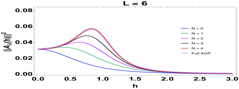
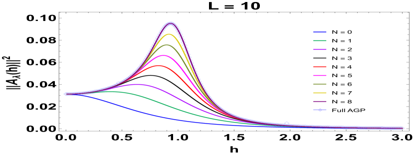
Figure 2: The AGP norm is compared by direct evaluation (5) and by solving (39) for different cutoffs. It can be seen that length of the vector $\vec{\alpha}$ in (39) is (a) $M=4$ for system size $6$,(b) $M=6$ for system size $8$ and (c) $M=8$ for system size $10$. The phase transition in the model at $h=1$ is also picked by the AGP, allowing for finite-size effects. The regulator is chosen to be $\mu=L2^{-L}$.

The finiteness of the Krylov space can be measured by evaluating the Lanczos coefficients numerically. These are shown in Fig. 3. It is observed that the Krylov space is much smaller than $\mathcal{D}^{2}-\mathcal{D}+1$, where $\mathcal{D}=2^{L}$ for system size $L$. This is a sign of the integrable nature of the system. It is interesting to note that the Lanczos coefficients do not depend on system size. The only contribution of the system size to the AGP is in terms of the number of Krylov basis operators required to describe the AGP. The coefficients of these operators (in the expression for AGP operator) are independent of the system size itself.

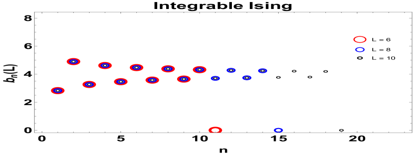
Figure 3: The Lanczos coefficients for system size $6$, $8$ and $10$ and $h=1$. The Krylov space is highly restricted, as only the first few Lanczos coefficients are non-zero. A nice feature of the model is that the Lanczos coefficients (and consequently the coefficients of the terms in the AGP operator) are independent of the system. The system size contributes by affecting the total number of terms in the expression of the AGP operator.

VIII.2 Weakly chaotic system

To study the truncation method in a weakly chaotic system, we turn our attention to the Lipkin-Meshkov-Glick (LMG) model Lipkin et al. (1965). This model is known to be weakly chaotic in the sense that it displays saddle-dominated scrambling. The classical limit of this model is integrable. However, it possesses one unstable saddle point, in whose vicinity orbits are chaotic. The effect of the saddle point has been studied from the perspective of Out-of-Time-Ordered-Correlator (OTOC)Xu et al. (2020) and Krylov complexity Bhattacharjee et al. (2022a). It was found that K-complexity is hypersensitive to the presence of unstable saddle points. The LMG model Hamiltonian is given below

$$H=\hat{X}+2J\hat{Z}^{2}$$ (60)

where $\{\hat{X},\hat{Y},\hat{Z}\}$ follow the $SU(2)$ algebra. We study this model for spin realizations $S=10$ and $30$ and compare the numerically evaluated AGP norm (6) with the one calculated from the Lanczos coefficients by taking a finite number of Krylov vectors to describe the AGP operator. The adiabatic deformation parameter $\lambda$ is taken to be $2J$ in this case. The intial operator is $\partial_{\lambda}H=\hat{Z}^{2}$. We begin by normalizing this operator and performing the Lanczos algorithm.

The first few operators in the Krylov basis are given below

$$\mathcal{O}_{0} =\frac{1}{z}\hat{Z}^{2}$$ (61)

$$\mathcal{O}_{1} =-\frac{1}{zb_{1}}\left(\hat{Z}\hat{Y}+\hat{Y}\hat{Z}\right)$$ (62)

$$\mathcal{O}_{2} =\frac{2}{zb_{1}b_{2}}\left(\hat{Y}^{2}-\hat{Z}^{2}+2J(\hat{X}\hat{Z}^{2}+\hat{Z}^{2}\hat{X}^{2}+2\hat{Z}\hat{X}\hat{Z}\right)$$

$$-\frac{b_{1}}{b_{2}z}\hat{Z}^{2}$$ (63)

$$\mathcal{O}_{3} =\frac{2}{zb_{1}b_{2}b_{3}}\Big{(}-2zb_{1}\mathcal{O}_{1}+2Jzb_{1}\{\hat{X},\mathcal{O}_{1}\}$$

$$-4J^{2}zb_{1}\{\hat{Z},\mathcal{O}_{1}\}-8J^{2}zb_{1}\hat{Z}\mathcal{O}_{1}\hat{Z}$$

$$-2J\left(\hat{Y}\hat{Z}\hat{X}+\hat{Z}\hat{X}\hat{Y}+\hat{Y}\hat{X}\hat{Z}+\hat{X}\hat{Z}\hat{Y}\right)$$

$$-4J(\hat{Z}\hat{X}\hat{Y}+\hat{Y}\hat{X}\hat{Z})\Big{)}+\frac{1}{zb_{3}}\left(\frac{b_{2}}{b_{1}}-\frac{b_{1}}{b_{2}}\right)\mathcal{O}_{1}$$ (64)

Here the norm of $\mathcal{O}_{0}$ is given by $z=\sqrt{|\hat{Z}^{2}|}=\frac{\sqrt{S(S+1)\left(3S^{2}+3S-1\right)}}{\sqrt{15}S^{2}}$ for arbitary spin $S$. To evaluate the regulated AGP norm, we pick the regulator $\mu=(2S+1)2^{-(2S+1)}$.

The operators become very complicated very quickly. The Lanczos coefficients are hard to evaluate for general spin $S$. The coefficients are dependent on both $S$ and $J$ (i.e. of $O(J)$). For the cases we study numerically ($S=10$ and $S=30$), the first few Lanczos coefficients are listed in Table. 1.

$b_{n}$	$S=10$	$S=30$
$n=1$	$0.12$	$0.038$
$n=2$	$\sqrt{0.074J^{2}+0.027}$	$\sqrt{0.0079J^{2}+0.0030}$
$n=3$	$J\sqrt{\frac{0.021J^{2}+0.053}{J^{2}+0.36}}$	$J\sqrt{\frac{0.0023J^{2}+0.0059}{J^{2}+0.38}}$

Table 1: Listing the first three Lanczos coefficients for $S=10$ and $S=30$ realizations of the LMG model

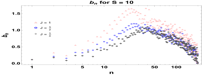
Figure 4: The full set of Lanczos coefficients are computed for $J=\{\frac{1}{4},\frac{1}{2},1\}$ for spin realisations (a) $S=10$ and (b) $S=30$. It can be observed that the number of Lanczos coefficients for (a) $S=10$ is $2M+1=201$, which gives us $M=100$. Similarly for (b) $S=30$, we have $2M+1=3659$, which gives us $M=1829$. Note that both satisfy the relation $K\leq\mathcal{D}^{2}-\mathcal{D}+1$, where $\mathcal{D}=21$ for $S=10$ and $\mathcal{D}=61$ for $S=30$.

We demonstrate numerically that the qualitative behavior of the AGP is captured by using (39) with the first few Lanczos coefficients. The matrix in (39) is constructed by cutting off at successive lengths $N$, and the AGP norm arising out of that is evaluated. This is done by considering (39) by terminating the matrix at $2N+1<2M+1$ and solving the matrix equation to evaluate $\alpha_{2k+1}$ where $0\leq k\leq N<M$. We perform this calculation for the two spin realizations of the LMG model ($S=10$ and $S=30$). The numerical results for the truncated AGP and the full AGP are given in Fig. 5 for $S=10$ and Fig. 5 for $S=30$.

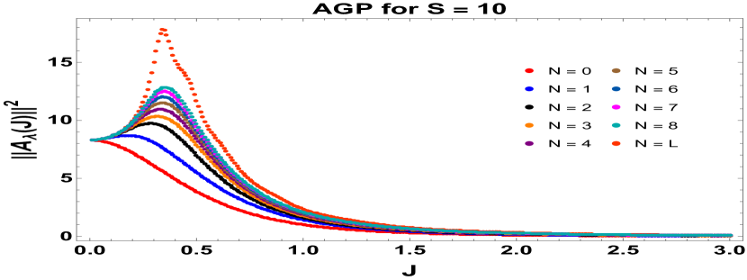
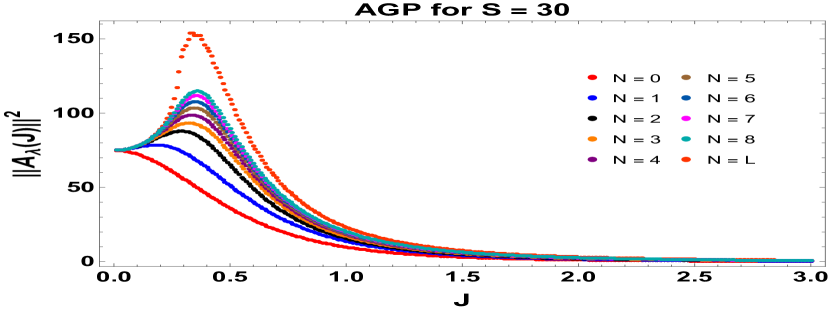
Figure 5: (a) The full AGP norm ($N=L$) and the truncated AGP norm evaluated at orders $N=0,\dots,8$ for the LMG model at a spin realisation $S=10$. Here the adiabatic deformation parameter is $\lambda=2J$. (b) The full AGP ($N=L$) norm and the truncated AGP norm ($N=0,\dots,8$) for $S=30$ realization of the LMG model.

One can find $M$ by evaluating the full set of Lanczos coefficients. The total number of Lanczos coefficients is the extent of the Krylov space. The full Krylov space is required to describe the AGP exactly. In Figs. 4 and 4, the full set of Lanczos coefficients are computed for the $S=10$ and $S=30$. The Krylov space ends once the Lanczos coefficients become $0$.

Note that there is a phase transition in the classical LMG model. The system transitions from an integrable to a chaotic phase at $J=\frac{1}{2}$. This can be observed via a classical calculation Bhattacharjee et al. (2022a), which corresponds to taking $S\rightarrow\infty$. The AGP (evaluated for finite $S$) reflects this phase transition since the AGP peaks close to $J=\frac{1}{2}$, as seen in Fig. 5.

VIII.3 Integrable Interacting model

We consider the $XXZ$ model with open boundary conditions Pandey et al. (2020). The Hamiltonian is the following

$$H=\sum_{i=1}^{L-1}\left(\sigma^{x}_{i+1}\sigma^{x}_{i}+\sigma^{y}_{i+1}\sigma^{y}_{i}\right)+\Delta\sum_{i=1}^{L-1}\sigma^{z}_{i+1}\sigma^{z}_{i}$$ (65)

This system is Bethe ansatz solvable Franchini (2017). However, the spectrum is not known, and thus the exact AGP is not available. Therefore, despite being integrable, it is different from the integrable non-interacting Ising model studied in a previous section.

We evaluate the AGP norm for this system via (6) and compare it to the result obtained from (39) by truncating successively at $N=0$ to $N=8$. We evaluate the AGP for $L=6,8$, and $10$. The numerical results are demonstrated in Fig. 6

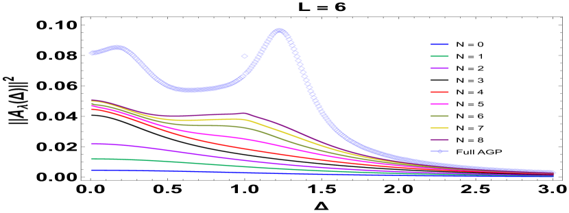
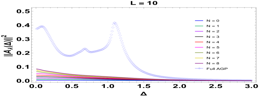
Figure 6: The AGP norm is compared by direct evaluation (6) and by solving (39) for different cutoffs and for system size (a) $L=6$, (b) $L=8$ and (c) $L=10$. The cutoffs are taken at $N=0,\dots,8$. It is evident that taking such a small number of Lanczos coefficients fails to capture the AGP to a decent reasonable extent. For a small system size $L=6$, the truncated AGP manages to barely replicate the behavior of the full AGP. However

From Fig. 6, it can be seen that the $N=8$ truncated AGP begins to show similar behavior to the full AGP. It is expected that the next few orders should be enough to replicate the qualitative nature of the AGP, though the full Krylov space will need to be spanned in order to exactly capture the AGP norm. The results become poorer with increasing $L$ (as seen in Fig. 6 and Fig. 6) since the Krylov space dimensions increase while $N$ remains the same.

VIII.4 Strongly Chaotic System

To study the truncation method in a strongly chaotic system, we focus on the chaotic Ising model.

$$H=\sum_{i=1}^{L}\sigma^{z}_{i}\sigma^{z}_{i+1}+h_{x}\sigma^{x}_{i}+h_{z}\sigma^{z}_{i}$$ (66)

with periodic boundary conditions. The model is known to be strongly chaotic for $h_{z}=\frac{\sqrt{5}+1}{4}$. The adiabatic deformation parameter is taken to be $h_{x}$.

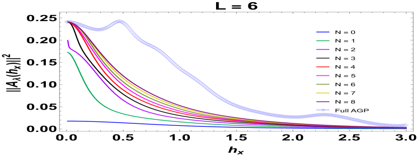
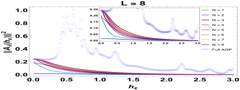
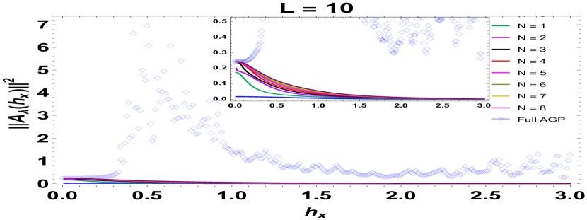
Figure 7: The AGP norm is compared by direct evaluation (6) and by solving (39) for different cutoffs and for system size (a) $L=6$, (b) $L=8$ and (c) $L=10$. The cutoffs are taken at $N=0,\dots,8$. It is evident that taking such a small number of Lanczos coefficients fails to capture the AGP to any reasonable extent. Inset in (b) and (c) shows a close-up of the results obtained via (39).

The strongly chaotic nature of the system is also reflected by the fact that using (39) up to $N=8$ fails to capture the exact AGP. The Krylov space dimension for such systems are close to the bound $K\leq\mathcal{D}^{2}-\mathcal{D}+1$ Barbón et al. (2019); Rabinovici et al. (2021, 2022b). Therefore, a much larger set of Lanczos coefficients are required to be fed into (39), which implies that the knowledge of a much larger set of Krylov vectors is needed.

Making a naïve qualitative comparison, we find that the truncated AGP best captures the full AGP for the integrable (free) model (59), less so for the weakly chaotic LMG model (60), even less so for the interacting $XXZ$ chain (65) and least so for the chaotic Ising model (66). This is related to the fact that the size of the Krylov space increases in that order, and so the truncated AGP (which spans a part of the full Krylov space) captures the AGP to a reduced level of success.

IX Probing Quantum Chaos: AGP and Operator Growth Hypothesis

The norm of the regulated Adiabatic Gauge Potential has been shown to be sensitive to the degree of chaos in the system Pandey et al. (2020). The sensitivity of the AGP norm is the highest when the regulator is chosen to be exponentially suppressed by the system size. Specifically, for a system of size $L$, the optimal choice of the regulator is found to be $\mu=L2^{-L}$. This choice also plays an important role in the scaling of the AGP norm with the system size. The rescaled AGP norm $||A_{\lambda}||^{2}/L$ scales exponentially $e^{L}$ for chaotic systems, as $L^{\beta}$ (for some constant $\beta$) for integrable interacting systems and nearly constant (up to exponentially suppressed corrections) for integrable non-interacting systems. We shall study some toy models and check these statements by using (29).

The first result we consider is the bound on the AGP norm. It was observed in Pandey et al. (2020) that the AGP norm cannot grow faster than $4^{M}$ (for system size $M$). In other words, it is bounded above by a term proportional to $\frac{1}{\mu^{2}}$. It is simpler to consider (24), and note that in the explicit form (88) one can use the fact that $\psi_{2n+1}(t)\leq 1\;\;\forall\;n$

$$||A_{\lambda}||^{2}\leq||\partial_{\lambda}H||^{2}\sum_{n=0}^{M}\int_{0}^{\infty}e^{-\mu(t+t^{\prime})}\mathrm{d}t\mathrm{d}t^{\prime}=\frac{M}{\mu^{2}}||\partial_{\lambda}H||^{2}$$ (67)

which confirms the bound. Here we have inserted the norm of the deforming operator $||\partial_{\lambda}H||^{2}$ by hand since (24) involves the normalized operator. Now, we begin by considering various types of autocorrelation functions and the corresponding AGP norms.

IX.0.1 Integrable: $b_{n}\sim\sqrt{n}$

The autocorrelation function we study is $\mathcal{C}(t)=e^{-\frac{t^{2}}{2}}$. This corresponds to the Heisenberg-Weyl type Hamiltonian Caputa et al. (2022). An autocorrelation function of this form is found when considering the growth of the $\sigma_{z}$ operator under the integrable non-interacting Ising model Hamiltonian (59) at criticality ($h=1$) Cao (2021). The result we get is the following

$$||A_{\lambda}(\mu)||^{2}=\frac{\sqrt{\frac{\pi}{2}}e^{\frac{\mu^{2}}{2}}\left(\mu^{2}+1\right)\text{Erfc}\left(\frac{\mu}{\sqrt{2}}\right)}{\mu}-1$$ (68)

where Erfc indicates the complementary error function. Taking an expansion around $\mu\rightarrow 0$ gives us the following asymptotic behavior

$$\frac{||A_{\lambda}(L)||^{2}}{K}\sim-\frac{2\mu^{2}}{3}+\frac{3}{4}\sqrt{\frac{\pi}{2}}\mu+\frac{\sqrt{\frac{\pi}{2}}}{2\mu}-1$$ (69)

It can be seen that the function (68) (and consequently (69)) grows as $e^{L}/L$ asymptotically. Considering the asymptotic growth of AGP with system size $L$ as the probe of chaotic dynamics Pandey et al. (2020), this result presents an apparent contradiction between the AGP and the Operator Growth Hypothesis results. This is also seen in the numerical result Fig. 8. The significance of this contradiction is not very clear at the moment. Part of the reason behind this may be that the AGP operator at $t=0$ is usually a highly non-local operator. The autocorrelation function considered here has mostly been studied by considering the time evolution of local operators. Whether locality is indeed of significance or not (in this context) remains to be seen.

There is also the issue of the norm of $\partial_{\lambda}H$. One may wonder if multiplying the result obtained from (29) by $||\partial_{\lambda}H||^{2}$ will change the scaling behavior. From most simple systems (such as the Ising model or the XXZ chain), it is straightforward to see that $||\partial_{\lambda}H||^{2}\sim O(L)$. This does not change our conclusions. Even if we allow the system to be such that $||\partial_{\lambda}H||^{2}\sim O(L^{\beta})$ for some $\beta>1$, the scaling with system size would still be exponential asymptotically.

IX.0.2 Chaotic: $b_{n}\sim n$

The autocorrelation function we study here corresponds to the asymptotically linear growth of Lanczos coefficients. The specific form of the Lanczos coefficients we choose are $b_{n}=\alpha\sqrt{n(n-1+\eta)}$ Parker et al. (2019). The corresponding autocorrelation function has the form $\mathcal{C}(t)=\operatorname{sech}(\alpha t)^{\eta}$. The corresponding AGP norm comes out to be

$$||A_{\lambda}(\mu)||^{2}=2^{\eta-2}\Big{(} \frac{\Gamma\left(\frac{1}{2}\left(\eta-\frac{\mu}{\alpha}\right)\right)\left(\Gamma\left(\frac{\alpha\eta+\mu}{2\alpha}\right)-\Gamma(\eta)\,_{2}\tilde{F}_{1}\left(\eta,\frac{1}{2}\left(\eta-\frac{\mu}{\alpha}\right);\frac{1}{2}\left(\eta-\frac{\mu}{\alpha}+2\right);-1\right)\right)}{\alpha\mu\Gamma(\eta)}$$

$$-\frac{2\,_{3}F_{2}\left(\eta,\frac{\eta}{2}+\frac{\mu}{2\alpha},\frac{\eta}{2}+\frac{\mu}{2\alpha};\frac{\eta}{2}+\frac{\mu}{2\alpha}+1,\frac{\eta}{2}+\frac{\mu}{2\alpha}+1;-1\right)}{(\alpha\eta+\mu)^{2}}\Big{)}$$ (70)

It is easy to see (by doing an expansion around $\mu=0$) that the leading order term in $\mu$ is $\propto\frac{1}{\mu}$. Therefore, the system demonstrates chaotic scaling since $\mu\sim e^{-L\log 2}$. This is compatible with the operator growth hypothesis. The same is reflected in the numerical result Fig. 8.

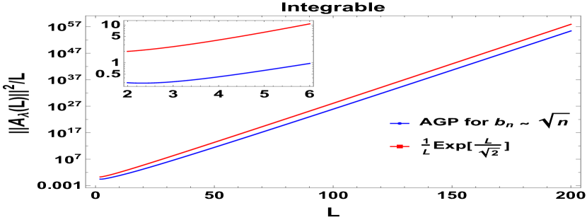
Figure 8: (a) The scaling of the AGP norm (Log plot) corresponding to a $\partial_{\lambda}H$ that gives rise to Lanczos coefficients that grow as $b_{n}\sim\sqrt{n}$, with system size $L$. According to the Operator Growth Hypothesis, this type of behavior (of the Lanczos coefficients) is associated with non-chaotic systems. (Inset): Scaling behavior for small $L$. (b) The scaling of the AGP norm (Log plot) for a $\partial_{\lambda}H$ corresponding to Lanczos coefficients that grow as $b_{n}\sim n$ asymptotically, with system size $L$. This type of behavior of the Lanczos coefficients is associated with chaotic systems, according to the Operator Growth Hypothesis. This plot corresponds to $\eta=5$ and $\alpha=4$. (Inset): Scaling behaviour for small $L$.

IX.0.3 Finite Krylov space: $SU(2)$ symmetry

Here we study a case where the Krylov space is highly restricted. This indicates strong integrability and has been found in real-life examples while studying the state complexity of many-body scars Bhattacharjee et al. (2022b). The Hamiltonian of such a system is given by

$$H=\alpha(J_{+}+J_{-})$$ (71)

where $J_{+}$ and $J_{-}$ are the raising and lowering operators in the $SU(2)$ algebra.

The autocorrelation function that we consider here (corresponding to the Hamiltonian described above) is given as $\mathcal{C}(t)=\cos^{L}\alpha t$ Caputa et al. (2022), where $L=2j$ (given the integer spin$-j$ representation of $SU(2)$). This autocorrelation function has the feature that the system size is a part of the autocorrelation function itself. The AGP norm turns out to have the following expression

$$||A_{\lambda}(L)||^{2}=\frac{2^{L-1}(\cosh(L\log(2))-\sinh(L\log(2)))}{L\left(2^{-L}L+i\alpha L\right)^{2}}\times$$

$$\Big{\{}2^{-L}L\,_{3}F_{2}\left(-L,f_{1}(L),f_{1}(L);f_{1}(L)+1,f_{1}(L)+1;-1\right)$$

$$-\left(2^{-L}L+i\alpha L\right)\,_{2}F_{1}\left(-L,f_{1}(L);f_{1}(L)+1;-1\right)\Big{\}}$$ (72)

where

$$f_{1}(L)=\frac{i2^{-L-1}L}{\alpha}-\frac{L}{2}$$ (73)

Since this is a complicated function, it is easier to simply plot the dependence of $A_{\lambda}(M)$ with $L$. Note that $L$ has to be even since $L=2j$ where $j$ is an integer spin. The result is given in Fig. 9. The growth is sub-exponential, which reflects the highly restricted nature of the Krylov space. It is also a sign of the integrability of the system.

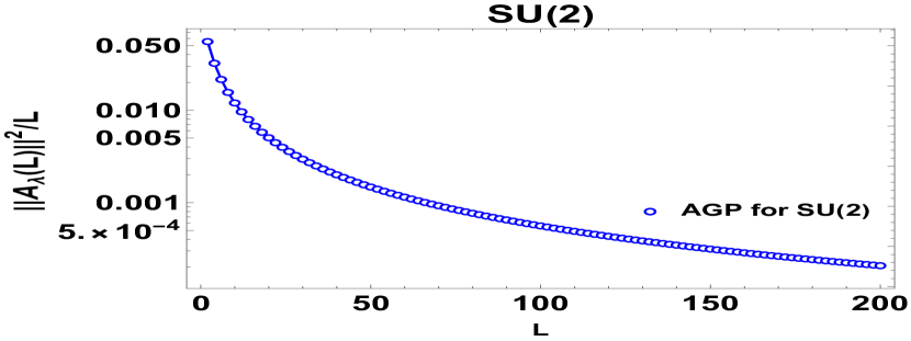
Figure 9: The AGP norm with the system size $L$ for the autocorrelation function corresponding to an $SU(2)$ Hamiltonian (71). It is observed that the growth is not exponential, indicating integrable dynamics.

IX.0.4 Constant Lanczos: $b_{n}\sim\alpha$

We consider a special kind of autocorrelation function Noh (2021), which gives rise to a set of Lanczos coefficients that are constant. This autocorrelation function is $\mathcal{C}(t)=\frac{J_{1}(2\alpha t)}{\alpha t}$, where $J$ is the Bessel function of the first kind. It follows from this that the Lanczos coefficients are $b_{n}=\alpha$, which is a constant. This is an integrable system according to the Operator Growth Hypothesis. The AGP norm for this autocorrelation function becomes

$$||A_{\lambda}||^{2}=\frac{\sqrt{\frac{4\alpha^{2}}{\mu^{2}}+1}-1}{\alpha^{2}}-\frac{2}{\mu\sqrt{4\alpha^{2}+\mu^{2}}}$$ (74)

A small $\mu$ expansion gives a series of the form $||A_{\lambda}||^{2}=\frac{1}{\alpha\mu}-\frac{1}{\alpha^{2}}+O(\mu)$, which implies that the norm scales as $\frac{1}{\mu}$ and is thus identified as chaotic according to the AGP probe. The two probes do not agree.

IX.0.5 Oscillatory Lanczos

A very interesting class of Lanczos coefficients are those that demonstrate different behavior for even and odd indices. In other words, $b_{2k+1}=f(k)$ and $b_{2k}=g(k)$, where $f$ and $g$ are different functions. There are some known autocorrelation functions that give rise to such Lanczos coefficients. One such autocorrelation function is $\mathcal{C}(t)=J_{0}(\alpha t)^{2}$. The AGP norm corresponding to this autocorrelation function is

$$||A_{\lambda}||^{2}=-\frac{2\left(E\left(-\frac{4\alpha^{2}}{\mu^{2}}\right)-\left(\frac{4\alpha^{2}}{\mu^{2}}+1\right)K\left(-\frac{4\alpha^{2}}{\mu^{2}}\right)\right)}{\pi\mu^{2}\left(\frac{4\alpha^{2}}{\mu^{2}}+1\right)}$$ (75)

where $K$ is the complete elliptic integral of the first kind and $E$ is the incomplete elliptic integral of the second kind. The AGP norm goes as

$$||A_{\lambda}||^{2}=\frac{\log\left(\frac{64\alpha^{2}}{\mu^{2}}\right)-2}{2\pi\alpha\mu}+O(\mu)$$ (76)

In terms of the system size $L$, the quantity $||A_{\lambda}||^{2}/L$ scales as $\frac{2^{L}}{L^{2}}$, which is a signature of chaotic behaviour. This is once more in contradiction with the result one expects from the Operator Growth Hypothesis.

Another closely related autocorrelation function is one that arises in the spin-$1/2$ $XY$ chain. The autocorrelation funcion $(\sigma^{x}_{0}(t)\sigma^{x}_{0})$ Brandt and Jacoby (1976) has the form $\mathcal{C}(t)=J_{0}(4t)^{2}+J_{1}(4t)^{2}$. This gives rise to another similar set of oscillating coefficients. The corresponding AGP norm takes the form.

$$||A_{\lambda}||^{2}=\frac{\left(\mu^{2}+32\right)K\left(-\frac{64}{\mu^{2}}\right)-\mu^{2}E\left(-\frac{64}{\mu^{2}}\right)}{8\pi\mu^{2}}$$ (77)

Again, this scales as $||A_{\lambda}||^{2}=\frac{-2\log(\mu)-4+\log(1024)}{4\pi\mu}+O(\mu)$. This is once again indicative of chaotic dynamics according to the AGP probe. The two methods (Operator Growth Hypothesis and AGP probe) are in conflict. The oscillatory Lanczos coefficients for both these autocorrelation functions are shown in Fig  .10.

From the results derived in this section, we discover that in some toy models, the Operator Growth Hypothesis and the AGP probe (for chaos) are in apparent contradiction. This is a fairly naïve study, and a more systematic and exhaustive approach is required to reach a conclusion. One point to note here is that the AGP operator is a special type of operator in view of locality (and analogously, in terms of sparseness in its’ matrix representation). The dependence of K-complexity on the type of operator choice is not very well understood yet. In that respect, the direct application of the Operator Growth Hypothesis that we undertake in this section may not be necessarily correct. Further investigation is required to reach a consensus. We defer it to future work.

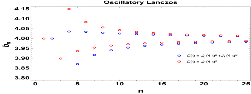
Figure 10: The Lanczos coefficients corresponding to the two autocorrelation functions $\mathcal{C}(t)=J_{0}(4t)^{2}+J_{1}(4t)^{2}$ and $\mathcal{C}(t)=J_{0}(4t)^{2}$ . The even and odd indexed coefficients show different behavior. These systems, according to the Operator Growth Hypothesis, are identified as integrable. The case is the opposite when using the AGP norm as the probe.

X Conclusions

The Adiabatic Gauge Potential has recently been considered as a probe of chaotic and integrable dynamics. Explicit expressions for the same, are hard to compute. It is only in certain integrable non-interacting systems that it has been possible to derive the expression. This difficulty arises partly because of the need to evaluate an infinite number of commutators. A way to bypass this process in some simple systems is by using a Gram-Schmidt-like orthonormalization procedure that brings down the number of computation steps to the bare minimum necessary Hatomura and Takahashi (2021).

We have discussed a formalism based on the Lanczos algorithm, which is one such orthonormalization procedure, and which allows us to evaluate the AGP operator and the (regularized) AGP norm by studying the time evolution of the adiabatic deformation operator. We show that using the Lanczos algorithm is akin to choosing an optimal basis vis-à-vis the variational approach for evaluating the AGP Sels and Polkovnikov (2017). Using this, we introduce a matrix equation that can be solved to evaluate the (Regularised) AGP operator and norm. We discuss a truncated approach in which we only evaluate a few operators and study how well it matches the actual result. We find that the matching is very good for integrable non-interacting systems, reasonably good for weakly chaotic systems, and very poor for strongly chaotic systems. The reason behind that is the relative sizes of the Krylov space (generated out of the Lanczos algorithm) in the three situations, respectively.

The Lanczos algorithm, however, has another interesting use. It is the central ingredient in the formalism of Krylov complexity which is used as a probe of chaotic dynamics. We derive an expression for the AGP norm in terms of an integral transform of the autocorrelation function and a derivative of Green’s function in the Krylov language. In the process, we find that the AGP response function provides a nice compatibility test between the Operator Growth Hypothesis and the Eigenstate Thermalization Hypothesis. We then evaluate the AGP for some systems with known autocorrelation functions. We compare the Operator Growth Hypothesis Parker et al. (2019) and the proposal for using AGP as a probe of chaos Pandey et al. (2020). We demonstrate that it is possible to construct some toy models where there is an apparent contradiction between the two probes.

There are various open questions that are of interest and require investigation. A natural future direction is to apply the analog of the Lanczos algorithm for open quantum systems Bhattacharya et al. (2022); Bhattacharjee et al. (2022c) to the AGP for open quantum systems Alipour et al. (2020). Regarding probing chaotic dynamics, the AGP and K-complexity are fundamentally different objects. The AGP probes the small-$\omega$ behavior (as seen from (20)) while the K-complexity probes the large-$\omega$ behavior as seen from the spectral function. This is part of the reason why AGP is, at times, more effective than K-complexity at probing phase transitions. However, the AGP norm can still be formally related to the machinery of K-complexity. It would be interesting to attempt to understand one in terms of the other. It would also be interesting to understand the scaling behavior of the AGP norm for different types of systems (chaotic/integrable/interacting, etc.) from a more fundamental perspective. It would also be interesting to study in detail the compatibility issues between AGP and K-complexity with respect to probing chaos. It would be of interest to apply the Lanczos formalism to derive the AGP operators of other, more complicated systems. Finally, it is of conceptual interest to extend the notion of adiabatic deformations to field theories and holography via the AGP.

Note added : Towards the finalizing stages of the manuscript, Ref.Takahashi and del Campo (2023) appeared on ArXiv, which proposes a nearly identical Lanczos formalism as ours.

XI Acknowledgements

The author would like to thank Xiangyu Cao, Jyotirmoy Mukherjee, Pratik Nandy, Tanay Pathak, Dario Rosa, and Samudra Sur for discussions on this and related projects, as well as for comments on this manuscript. The author is supported by the Ministry of Human Resource Development, Government of India, via the Prime Ministers’ Research Fellowship.

Appendix A Derivation of the Expressions for the AGP

In this Appendix, we describe the steps (that we skipped in the main text) regarding the derivation of the expression for the AGP norm.

In the discussion of the response function, we obtained the expression for the $\overline{|}f_{\lambda}(\omega)|^{2}$. We note that the AGP norm is written as Pandey et al. (2020)

$$||A_{\lambda}||^{2}=\int_{-\infty}^{\infty}\mathrm{d}\omega\frac{\omega^{2}}{(\omega^{2}+\mu^{2})^{2}}\overline{|f_{\lambda}(\omega)|}^{2}\,.$$ (78)

Using (78) we find the expression for the AGP. The integral over $\omega$ for the first term in (27) is

$$\int_{-\infty}^{\infty}\mathrm{d}\omega\frac{\omega^{2}}{(\omega^{2}+\mu^{2})^{2}}e^{i\omega t}=\frac{\pi e^{-\mu|t|}}{2\mu}-\frac{1}{2}\pi|t|e^{-\mu|t|}$$ (79)

The second term in (27) vanishes due to the $\delta(\omega)$ (note that $\mu>0$). Therefore the expression for the AGP norm becomes

$$||A_{\lambda}||^{2}=\frac{1}{2}\int_{0}^{\infty}\mathrm{d}t\left(\frac{1}{\mu}-t\right)\mathcal{C}(t)e^{-\mu t}\,.$$ (80)

where we have changed the limits on the $t$ integral from $\{-\infty,\infty\}$ to $\{0,\infty\}$. Without the $\frac{1}{\mu}$ piece in the integrand, the AGP norm is simply the negative of the Laplace transform of the function $t\mathcal{C}(t)$. . The expression (80) can also be obtained from (93) by an appropriate change of variables.

A.1 An alternative expression

We demonstrate that there is an alternative expression in terms of the difference between two shifted autocorrelation functions, which we derive below.

We begin with the following expression

$$||A_{\lambda}||^{2} =\frac{1}{\mathcal{D}}\sum_{m\neq n}|\bra{m}A_{\lambda}\ket{n}|^{2}$$

$$=\frac{1}{\mathcal{D}}\sum_{m\neq n}\frac{\omega^{2}_{mn}}{(\mu^{2}+\omega^{2}_{mn})^{2}}|\bra{m}\partial_{\lambda}H\ket{n}|^{2}\,.$$ (81)

where $\mathcal{D}$ is the dimension of the Hilbert space. It is straightforward to show that this expression can be obtained from (20) directly.

From the expression (22), we now evaluate $||A_{\lambda}||^{2}$. The expression we obtain is

$$\bra{m}A_{\lambda}\ket{k}=-\sum_{n=0}^{M}\alpha_{2n+1}\bra{m}\mathcal{O}_{2n+1}\ket{k}\,.$$ (82)

Note that $\alpha_{2n+1}$ is the Laplace transform of $i^{2n+1}\psi_{2n+1}$. It is simple to note that $\alpha^{\ast}_{2n+1}=-\alpha_{2n+1}$ by using the fact that $\psi_{2n+1}(t)$ are real functions of $t$. Noting that all the odd-indexed Krylov basis operators are anti-hermitian, the complex conjugate of (82) is given by

$$\bra{m}A_{\lambda}\ket{k}^{\ast} =-\sum_{n=0}^{M}\alpha^{\ast}_{2n+1}\bra{k}\mathcal{O}_{2n+1}^{\dagger}\ket{m}$$

$$=-\sum_{n=0}^{M}\alpha_{2n+1}\bra{k}\mathcal{O}_{2n+1}\ket{m}\mathrm{d}t$$ (83)

Therefore, one can now write an expression for the regularized AGP matrix element as

$$|\bra{m}A_{\lambda}\ket{k}|^{2}=\sum_{n,n^{\prime}=0}^{M} \alpha_{2n+1}\alpha_{2n^{\prime}+1}\bra{k}\mathcal{O}_{2n+1}\ket{m}$$

$$\times\bra{m}\mathcal{O}_{2n^{\prime}+1}\ket{k}$$ (84)

Finally, we have to sum over the eigenstates $\ket{m},\ket{k}$ while keeping $m\neq k$. This leads us to the following expression

$$\sum_{m\neq k}|\bra{m}A_{\lambda}\ket{k}|^{2} =\sum_{k}\sum_{n,n^{\prime}=0}^{M}\alpha_{2n+1}\alpha_{2n^{\prime}+1}$$

$$\times\bra{k}\mathcal{O}_{2n+1}\left(\mathbf{I}-\ket{k}\bra{k}\right)\mathcal{O}_{2n^{\prime}+1}\ket{k}$$

$$=\sum_{k}\sum_{n,n^{\prime}=0}^{M}\alpha_{2n+1}\alpha_{2n^{\prime}+1}$$

$$\times\bra{k}\mathcal{O}_{2n+1}\mathcal{O}_{2n^{\prime}+1}\ket{k}$$ (85)

where in the last step, we have used $\bra{k}\mathcal{O}_{2n+1}\ket{k}=0$.

Lastly, we use the fact that

$$\sum_{k}\bra{k}\mathcal{O}_{2n+1}\mathcal{O}_{2n^{\prime}+1}\ket{k}=-\text{Tr}\{\mathbf{1}\}(\mathcal{O}_{2n+1}|\mathcal{O}_{2n^{\prime}+1})$$ (86)

with $\text{Tr}(\mathbf{1})=\mathcal{D}$ and that all the Krylov basis operators $\mathcal{O}_{n}$ are orthonormal to each other. This gives us

$$||A_{\lambda}||^{2}=-\sum_{n=0}^{M}\alpha_{2n+1}^{2}$$ (87)

From the expression (23), we find that this expression may be written as

$$||A_{\lambda}||^{2}=\sum_{n=0}^{M}\int_{0}^{\infty}\psi_{2n+1}(t)\psi_{2n+1}(t^{\prime})e^{-\mu(t+t^{\prime})}\mathrm{d}t\mathrm{d}t^{\prime}$$ (88)

In order to arrive at the alternative expression, it is helpful to define the following term

$$\beta_{n}=\frac{1}{2}\int_{t=-\infty}^{\infty}\text{sgn}(t)i^{n}\left\{\begin{aligned} &1\;\;n\in\text{odd}\\ &i\;\;n\in\text{even}\end{aligned}\right\}e^{-\mu|t|}\psi_{n}(t)\mathrm{d}t$$ (89)

Note that since $\beta_{2n}=0$ and $\beta_{2n+1}=\alpha_{2n+1}$, we can rewrite the AGP norm as

$$||A_{\lambda}||^{2}=-\sum_{n=0}^{K}\beta^{2}_{n}$$ (90)

This expression, when expanded out, becomes

$$||A_{\lambda}||^{2}=\frac{1}{4}\sum_{n=0}^{K}\int_{-\infty}^{\infty}\text{sgn}(t)\text{sgn}(t^{\prime})\psi_{n}(t)\psi_{n}(t^{\prime})e^{-\mu|t|-\mu|t^{\prime}|}\mathrm{d}t\mathrm{d}t^{\prime}\,.$$ (91)

Note the sum $\sum_{n=0}^{K}\psi_{n}(t)\psi_{n}(t^{\prime})$. This sum equals $\psi_{0}(t-t^{\prime})$ by definition, which is the autocorrelation function $\mathcal{C}(t-t^{\prime})$. Intuitively, it follows from the fact that the sum of the product of two eigen-solutions of a differential equation is Green’s function. This allows us to write the AGP norm as

$$||A_{\lambda}||^{2}=\frac{1}{4}\int_{-\infty}^{\infty}\text{sgn}(t)\text{sgn}(t^{\prime})\mathcal{C}(t-t^{\prime})e^{-\mu(|t|+|t^{\prime}|)}\mathrm{d}t\mathrm{d}t^{\prime}$$ (92)

It is worth simplifying this expression further. To do that, we simply turn the integrals over $t$ and $t^{\prime}$ to the limits $\{0,\infty\}$. This gives us

$$||A_{\lambda}||^{2}=\frac{1}{2}\int_{0}^{\infty}\left(\mathcal{C}(t-t^{\prime})-\mathcal{C}(t+t^{\prime})\right)e^{-\mu(t+t^{\prime})}\mathrm{d}t\mathrm{d}t\,.$$ (93)

where we have used the fact that $\mathcal{C}$ is an even function.

A.2 AGP as a product of Lanczos coefficients

The moments of the autocorrelation function and the Lanczos coefficients contain the same information, repackaged in a different way Parker et al. (2019). An iterative algorithm Viswanath and Müller (1994a) can be used to obtain one from the other. Due to that, it is instructive to consider the expression (29) and use the expansion of autocorrelation function in terms of moments Parker et al. (2019). This gives us the following result

$$||A_{\lambda}||^{2}=\sum_{n}\frac{n(-1)^{n+1}m_{2n}}{\mathbf{\mu}^{2n+2}}$$ (94)

Therefore, the knowledge of the moments of the autocorrelation function is equivalent to the knowledge of the AGP norm.

It is also possible to evaluate it in terms of the Lanczos coefficients themselves. In order to achieve that, we note the following relation between the moments $m_{2n}$ and the Lanczos coefficients $b_{n}$. The relation between moments and Lanczos coefficients is obtained via a product over Dyck paths. Using the expression in Parker et al. (2019), we write the AGP norm as

$$||A_{\lambda}||^{2}=\sum_{n}\frac{n(-1)^{n+1}}{\mu^{2n+2}}\sum_{\{c_{k}\}\in\mathcal{F}_{n}}\prod^{2n}_{k=1}b_{(c_{k}+c_{k-1})/2}$$ (95)

The indices $c_{k}\geq\frac{1}{2}$ and $c_{0}=c_{2n}=\frac{1}{2}$, with the constraint that $|c_{k}-c_{k+1}|=1$. The set of such paths is denoted by $\mathcal{F}_{n}$. The number of Dyck paths for a fixed $n$ is given by the Catalan number $C_{n}=\frac{\Gamma(2n+1)}{\Gamma(n+1)\Gamma(n+2)}$. As mentioned in Parker et al. (2019), this provides a set of bounds on the moments $m_{2n}$, which is given by $b_{1}^{2}b_{2}^{2}\dots b_{n}^{2}\leq m_{2n}\leq\text{max}_{k=1}^{n}(b_{k}^{2})C_{n}$.

Appendix B Derivation of AGP operator for the analytic cases

In this Appendix, we detail the derivation of the AGP operator for the cases considered in the main text. We begin with considering the simple $2$-level system (40).

1. The $2$-level system

We employ the Lanczos algorithm to determine the AGP operator (22). The steps are outlined below

• Consider the Hamiltonian $H=\lambda\sigma^{z}+\Delta\sigma^{x}$ and the intial operator $\mathcal{O}_{0}=\sigma^{z}\equiv\partial_{\lambda}H$. Note that this operator is normalized.

• The first Krylov basis operator is obtained as $b_{1}\mathcal{O}_{1}=[H,\mathcal{O}_{0}]$. This gives us $\mathcal{O}_{1}=-i\sigma^{y}$ and $b_{1}=2\Delta$.

• The second Krylov basis operator is written as $b_{2}\mathcal{O}_{2}=[H,\mathcal{O}_{1}]-b_{1}\mathcal{O}_{0}$. This gives us $b_{2}=2\lambda$ and $\mathcal{O}_{2}=-\sigma^{x}$.

• The third Krylov basis operator turns out to be $b_{3}\mathcal{O}_{3}=[H,\mathcal{O}_{2}]-b_{2}\mathcal{O}_{1}=0$. Therefore, we find that $b_{3}=0$, and the Lanczos algorithm terminates.

Therefore, the Krylov basis has three independent basis elements, denoted by $\mathcal{O}_{0},\mathcal{O}_{1}$, and $\mathcal{O}_{2}$. The dimensions of the Krylov space is $3$, which saturates the bound $K\leq\mathcal{D}^{2}-\mathcal{D}+1$, where $K$ is the dimension of the Krylov space and $\mathcal{D}$ is the dimension of the Hilbert space. In this case $\mathcal{D}=2$ and $K=3$.

Now that we have obtained the Krylov basis vectors, we turn out attention to the wavefunctions. These are obtained via the recursive relation (13). Note that (22) tells us that only the odd indexed wavefunctions contribute to the AGP operator. Therefore, we only need to consider $\psi_{1}$, since $\psi_{0},\psi_{2}$ do not contribute and all other $\psi_{n}\,\forall\,n\geq 3$ are $0$. From (13), it can be easily seen that

$$\psi_{1}=-\frac{1}{b_{1}}\partial_{t}\psi_{0}(t)$$ (96)

Thus the AGP operator is written as (using (22))

$$A_{\lambda} =-\left(\int_{0}^{\infty}ie^{-\mu t}\psi_{1}(t)\mathrm{d}t\right)\mathcal{O}_{1}$$

$$=\frac{1}{b_{1}}\left(\int_{0}^{\infty}ie^{-\mu t}\partial_{t}\psi_{0}(t)\mathrm{d}t\right)\mathcal{O}_{1}$$ (97)

Knowing the autocorrelation function $\psi_{0}(t)$ allows us to evaluate the integral above. Integrating by parts turns this integral into an integral over $\psi_{0}(t)$ only, which can be evaluated easily. The result turns out to be

$$A_{\lambda} =-\frac{i}{b_{1}}(-i\sigma^{y})\frac{4\Delta^{2}}{4\Delta^{2}+4\lambda^{2}}$$

$$=-\frac{1}{2}\frac{\Delta}{\Delta^{2}+\lambda^{2}}\sigma^{y}$$ (98)

This result matches with the expression derived in del Campo et al. (2012), as expected.

2. A 2-qubit system

In this section, we derive the AGP operator for the Hamiltonian (45)

$$H(\lambda)=-\left(\sigma^{1}_{x}\sigma^{2}_{x}+\sigma^{1}_{z}\sigma^{2}_{z}\right)-\varepsilon(1-\lambda)\left(\sigma^{1}_{z}+\sigma^{2}_{z}\right)\,.$$ (99)

The steps are the same as discussed for the $2-$ level system, so we shall omit them here. The results for the Krylov basis operators are as follows

$$\mathcal{O}_{0} =\frac{\partial_{\lambda}H}{\sqrt{(\partial_{\lambda}H|\partial_{\lambda}H)}}=\frac{1}{\sqrt{2}}(\sigma^{1}_{z}+\sigma^{2}_{z})$$ (100)

$$b_{1}\mathcal{O}_{1} =\frac{1}{b_{1}}\left([H,\mathcal{O}_{0}]\right)=\frac{i}{\sqrt{2}}(\sigma^{1}_{x}\sigma^{2}_{y}+\sigma^{1}_{y}\sigma^{2}_{x})$$ (101)

$$\mathcal{O}_{2} =\frac{1}{b_{2}}\left([H,\mathcal{O}_{1}]-b_{1}\mathcal{O}_{0}\right)=\frac{1}{\sqrt{2}}\left(\sigma^{1}_{y}\sigma^{2}_{y}-\sigma^{1}_{x}\sigma^{2}_{x}\right)$$ (102)

$$b_{3}\mathcal{O}_{3} =[H,\mathcal{O}_{2}]-b_{2}\mathcal{O}_{1}=0$$ (103)

The Lanczos coefficients are $b_{1}=2,\,b_{2}=4|\varepsilon(1-\lambda)|$ and $b_{n}=0\,\,\forall n\geq 3$. Therefore, the AGP operator is proportional to $\mathcal{O}_{1}$. Using the expression for the autocorrelation function (46), we have the following expression for $\alpha_{1}$

$$-i\int_{0}^{\infty}e^{-\mu t}\psi_{1}(t)\mathrm{d}t =\frac{i}{b_{1}}\int_{0}^{\infty}e^{-\mu t}\partial_{t}\psi_{0}(t)\mathrm{d}t$$

$$=-\frac{2i}{4+16\varepsilon^{2}(1-\lambda)^{2}+\mu^{2}}$$ (104)

It is possible to set $\mu\rightarrow 0$ in this expression, as the Hamiltonian (45) is non-degenerate. This gives us

$$A_{\lambda}=-\frac{i\sqrt{2}}{4(1+4\varepsilon^{2}(1-\lambda)^{2})}\left(\sigma^{1}_{x}\sigma^{2}_{y}+\sigma^{1}_{y}\sigma^{2}_{x}\right)$$ (105)

This result does not match exactly with Petiziol et al. (2018) since we started with a normalized $\partial_{\lambda}H$. To obtain the result derived in Petiziol et al. (2018), we must multiply this AGP operator by the norm of $\partial_{\lambda}H=\sqrt{2}\varepsilon$. This gives us the AGP operator

$$A_{\lambda}=-\frac{i\varepsilon}{2(1+4\varepsilon^{2}(1-\lambda)^{2})}\left(\sigma^{1}_{x}\sigma^{2}_{y}+\sigma^{1}_{y}\sigma^{2}_{x}\right)$$ (106)

which is the result derived in Petiziol et al. (2018).

3. A 4-body system

We consider the Hamiltonian (49) and employ the Lanczos algorithm. Our starting point is the intial operator (normalized) $\partial_{\lambda}H(\lambda)=\frac{1}{\sqrt{2}}(\sigma^{z}_{1}+\sigma^{z}_{2})$. The Krylov basis vectors are evaluated in the same way as before, and their expressions are listed below

$$\mathcal{O}_{0} =\frac{1}{\sqrt{2}}\left(\sigma^{z}_{1}+\sigma^{z}_{2}\right)$$ (107)

$$\mathcal{O}_{1} =-\frac{i}{2}\left(\sigma^{x}_{0}\sigma^{y}_{1}+\sigma^{x}_{1}\sigma^{y}_{2}+\sigma^{y}_{1}\sigma^{x}_{2}+\sigma^{y}_{2}\sigma^{x}_{3}\right)$$ (108)

$$\mathcal{O}_{2} =\frac{1}{\sqrt{8+10\lambda^{2}}}\left(2\sigma^{x}_{0}\sigma^{z}_{1}\sigma^{x}_{2}+2\sigma^{x}_{1}\sigma^{z}_{2}\sigma^{x}_{3}+\lambda\left(2\sigma^{y}_{1}\sigma^{y}_{2}-2\sigma^{x}_{1}\sigma^{x}_{2}-\sigma^{x}_{0}\sigma^{x}_{1}-\sigma^{x}_{2}\sigma^{x}_{3}\right)\right)$$ (109)

$$\mathcal{O}_{3} =\frac{6\lambda^{2}}{b_{2}b_{3}}\left(\mathcal{O}_{1}+i(\sigma^{x}_{0}\sigma^{y}_{1}+\sigma^{y}_{2}\sigma^{x}_{3})\right)+\frac{8i\lambda}{b_{2}b_{3}}\left(\sigma^{x}_{0}\sigma^{z}_{1}\sigma^{y}_{2}+\sigma^{y}_{1}\sigma^{z}_{2}\sigma^{x}_{3}\right)$$ (110)

$$\mathcal{O}_{4} =\frac{6\lambda^{2}b_{2}}{b_{2}b_{3}b_{4}}\mathcal{O}_{2}+\frac{(12\lambda^{3}+\lambda b_{3}^{2})}{b_{2}b_{3}b_{4}}\left(\sigma^{x}_{0}\sigma^{x}_{1}+\sigma^{x}_{2}\sigma^{x}_{3}\right)+\frac{(32\lambda-2\lambda b_{3}^{2})}{b_{2}b_{3}b_{4}}\sigma^{y}_{1}\sigma^{y}_{2}+\frac{2\lambda b_{3}}{b_{2}b_{4}}\sigma^{x}_{1}\sigma^{x}_{2}$$

$$+\frac{(4\lambda^{2}-2b_{3}^{2})}{b_{2}b_{3}b_{4}}\left(\sigma^{x}_{0}\sigma^{z}_{1}\sigma^{x}_{2}+\sigma^{x}_{1}\sigma^{z}_{2}\sigma^{x}_{3}\right)-\frac{32\lambda}{b_{2}b_{3}b_{4}}\sigma^{x}_{0}\sigma^{z}_{1}\sigma^{z}_{2}\sigma^{x}_{3}$$ (111)

$$\mathcal{O}_{5} =\left(\frac{6\lambda^{2}-b_{4}^{2}}{b_{4}b_{5}}\right)\mathcal{O}_{3}+\left(\frac{6\lambda^{2}b_{2}^{2}+16\lambda^{2}-8b_{3}^{2}-4\lambda^{2}b_{3}^{2}}{b_{2}b_{3}b_{4}b_{5}}\right)\mathcal{O}_{1}+\frac{24i\lambda^{4}}{b_{2}b_{3}b_{4}b_{5}}\left(\sigma^{x}_{0}\sigma^{y}_{1}+\sigma^{y}_{2}\sigma^{x}_{3}\right)$$

$$+\left(\frac{6i\lambda^{2}b_{3}^{2}-64i\lambda^{2}}{b_{2}b_{3}b_{4}b_{5}}\right)\left(\sigma^{x}_{1}\sigma^{y}_{2}+\sigma^{y}_{1}\sigma^{x}_{2}\right)+\left(\frac{128i\lambda-8i\lambda b_{3}^{2}+8i\lambda^{3}}{b_{2}b_{3}b_{4}b_{5}}\right)\left(\sigma^{x}_{0}\sigma^{z}_{1}\sigma^{y}_{2}+\sigma^{y}_{1}\sigma^{z}_{2}\sigma^{x}_{3}\right)$$ (112)

$$\mathcal{O}_{6} =\left(\frac{6\lambda^{2}-b_{4}^{2}-b_{5}^{2}}{b_{5}b_{6}}\right)\mathcal{O}_{4}+\left(\frac{2\lambda^{2}b_{3}^{2}-b_{4}^{2}b_{3}^{2}+6\lambda^{2}b_{2}^{2}+16\lambda^{2}-8b_{3}^{2}}{b_{3}b_{4}b_{5}b_{6}}\right)\mathcal{O}_{2}$$

$$+\left(\frac{2\sqrt{2}(6\lambda^{2}b_{2}^{2}+80\lambda^{2}-24\lambda^{4}-8b_{3}^{2}-10\lambda^{2}b_{3}^{2})}{b_{2}b_{3}b_{4}b_{5}b_{6}}\right)\mathcal{O}_{0}-\lambda^{3}\left(\frac{24b_{3}^{2}-256}{b_{2}b_{3}b_{4}b_{5}b_{6}}\right)\left(\sigma^{y}_{1}\sigma^{y}_{2}-\sigma^{x}_{1}\sigma^{x}_{2}\right)$$

$$+\left(\frac{384\lambda^{2}-28\lambda^{2}b_{3}^{2}-32\lambda^{4}}{b_{2}b_{3}b_{4}b_{5}b_{6}}\right)\left(\sigma^{x}_{0}\sigma^{z}_{1}\sigma^{x}_{2}+\sigma^{x}_{1}\sigma^{z}_{2}\sigma^{x}_{3}\right)+\frac{48\lambda^{5}}{b_{2}b_{3}b_{4}b_{5}b_{6}}\left(\sigma^{x}_{0}\sigma^{x}_{1}+\sigma^{x}_{2}\sigma^{x}_{3}\right)$$

$$+\left(\frac{512\lambda-32\lambda b_{3}^{2}+32\lambda^{3}}{b_{2}b_{3}b_{4}b_{5}b_{6}}\right)\sigma^{y}_{1}\sigma^{y}_{2}-\left(\frac{512\lambda-32\lambda b_{3}^{2}+32\lambda^{3}}{b_{2}b_{3}b_{4}b_{5}b_{6}}\right)\sigma^{x}_{0}\sigma^{z}_{1}\sigma^{z}_{2}\sigma^{x}_{3}$$ (113)

The Lanczos coefficients obtained corresponding to these Krylov vectors are given as follows

$$b_{1} =2\sqrt{2}$$ (114)

$$b_{2} =\sqrt{8+10\lambda^{2}}$$ (115)

$$b_{3} =\sqrt{\frac{2\lambda^{2}\left(9\lambda^{2}+32\right)}{5\lambda^{2}+4}}$$ (116)

$$b_{4} =2\sqrt{\frac{72\lambda^{6}+202\lambda^{4}+448\lambda^{2}+512}{45\lambda^{4}+196\lambda^{2}+128}}$$ (117)

$$b_{5} =2\lambda\sqrt{\frac{(5\lambda^{2}+4)(16-9\lambda^{2})^{2}}{\left(9\lambda^{2}+32\right)\left(36\lambda^{6}+101\lambda^{4}+224\lambda^{2}+256\right)}}$$ (118)

$$b_{6} =4\lambda\sqrt{\frac{\left(9\lambda^{2}+32\right)\left(\lambda^{4}+2\lambda^{2}+4\right)}{36\lambda^{6}+101\lambda^{4}+224\lambda^{2}+256}}$$ (119)

Using (39) now allows us to obtain the expression (50).

Appendix C Gauge constraint for regularized AGP

In this section, we shall derive the gauge condition satisfied by the regularized AGP operator. The regularised AGP operator may be written as

$$A_{\lambda}=-\frac{1}{2}\int_{-\infty}^{\infty}\text{sgn}(t)e^{-\mu|t|}\partial_{\lambda}H(t)\mathrm{d}t$$ (120)

Calculating the expectation value between two eigenstates $\bra{m}$ and $\ket{n}$ (with $m\neq n$) gives us the expression

$$\bra{m}A_{\lambda}\ket{n}=-\frac{i\omega_{mn}}{\mu^{2}+\omega_{mn}^{2}}\bra{m}\partial_{\lambda}H\ket{n}$$ (121)

where $\omega_{mn}=E_{m}-E_{n}$. We note the following

$$\omega_{mn}^{2}\bra{m}A_{\lambda}\ket{n}=\bra{m}[H,[H,A_{\lambda}]]\ket{n}$$

$$-i\omega_{mn}\bra{m}\partial_{\lambda}H\ket{n}=-i\bra{m}[H,\partial_{\lambda}H]\ket{n}$$ (122)

Therefore, using it, one can note that this expression reduces to

$$\bra{m}[H,i\partial_{\lambda}H+[H,A_{\lambda}]]+\mu^{2}A_{\lambda}\ket{n}=0$$ (123)

In matrix notation, this expression can be written as

$$[H,[H,i\partial_{\lambda}H+[H,A_{\lambda}]]+\mu^{2}A_{\lambda}]=0$$ (124)

However, this gauge constraint is redundant in the sense that it generates an over-complete set of equations for the coefficients $\alpha$. The reason behind it is the fact that the following equation holds

$$[H,i\partial_{\lambda}H+[H,A_{\lambda}]]+\mu^{2}A_{\lambda}=0$$ (125)

which can be seen by using (33) and (34).

Appendix D Integrable non-interacting model

We evaluate an approximate analytical expression for the AGP for the following system

$$H=\frac{1}{2}\sum_{i}\sigma^{x}_{i}\sigma^{x}_{i+1}+h\sigma^{z}_{i}$$ (126)

This is an Ising chain. We shall evaluate the AGP at criticality (i.e., $h=1$). The explicit AGP operator has been derived by a Jordan-Wigner transformation to a free fermion chain del Campo et al. (2012). It has also been derived via the Lanczos approach Takahashi and del Campo (2023). In this section, we use the autocorrelation function to derive the AGP norm. We use the following result Brandt and Jacoby (1976) for the Ising chain at criticality.

$$\mathcal{C}_{l,m}(t)\equiv(\sigma^{z}_{l}(t)\sigma^{z}_{m})$$

$$=(J_{2l-2m}(2t))^{2}-J_{2l-2m+1}(2t)J_{2l-2m-1}(2t)$$ (127)

where $J_{\nu}(t)$ is the Bessel function of first kind. The autocorrelation function for the deformation operator $\sum_{i}\sigma^{z}_{i}$ is

$$\mathcal{C}(t)=\sum_{l=1}^{L}\sum_{m=1}^{L}\mathcal{C}_{l,m}(t)$$ (128)

To evaluate the AGP norm, we need the following integrals

$$\mathbf{I}_{1}(\nu)=\int_{0}^{\infty}J_{\nu}(2t)^{2}e^{-\mu t}\mathrm{d}t$$

$$=\frac{16^{\nu}\mu^{-2\nu-1}\Gamma\left(\nu+\frac{1}{2}\right)^{2}\,_{2}\tilde{F}_{1}\left(\nu+\frac{1}{2},\nu+\frac{1}{2};2\nu+1;-\frac{16}{\mu^{2}}\right)}{\pi}$$ (129)

and

$$\mathbf{I}_{2}(\nu)=\int_{0}^{\infty}J_{\nu-1}(2t)J_{\nu+1}(2t)e^{-\mu t}\mathrm{d}t=((2\nu)!)^{2}\mu^{-2\nu-1}$$

$$\times\,_{4}\tilde{F}_{3}\left(\nu+\frac{1}{2},\nu+\frac{1}{2},\nu+1,\nu+1;\nu,\nu+2,2\nu+1;-\frac{16}{\mu^{2}}\right)$$ (130)

where $\,{}_{p}\tilde{F}_{q}$ is the regularized hypergeometric function with $p,q$ parameters Weisstein (2003).

The regulated AGP norm is written as

$$||A_{\lambda}(1)||^{2}=\sum_{l,m}\left(\frac{1}{\mu}+\partial_{\mu}\right)(\mathbf{I}_{1}(2l-2m)-\mathbf{I}_{2}(2l-2m))$$ (131)

which evaluates to (where $\nu=2l-2m$)

$$||A_{\lambda}(1)||^{2}=\sum_{l,m=1}^{L}\frac{(\nu+1)(2\nu)!\mu^{-2(\nu+2)}}{\Gamma(\nu+2)^{2}}$$

$$\times\Bigg{\{}-\mu^{2}\nu\,_{3}F_{2}\left(\nu+\frac{1}{2},\nu+\frac{1}{2},\nu+1;\nu+2,2\nu+1;-\frac{16}{\mu^{2}}\right)$$

$$-\frac{4(\nu+1)(2\nu+1)}{\nu+2}$$

$$\times\,_{3}F_{2}\left(\nu+\frac{3}{2},\nu+\frac{3}{2},\nu+2;\nu+3,2\nu+2;-\frac{16}{\mu^{2}}\right)\Bigg{\}}$$ (132)

This sum is highly non-trivial, so we leave the expression as it is. At least formally, this presents an analytical expression for the AGP norm of the Ising chain (126) at criticality $h=1$. However, it is important to note that this expression is approximate. That is due to the fact (as explained in detail in Brandt and Jacoby (1976)) that the autocorrelation function (127) holds only for $l,m$ away from the boundary of the chain. Since that is not the case here, some of the terms in the sum (132) will pick up errors.

References

- Hatomura and Takahashi (2021) Takuya Hatomura and Kazutaka Takahashi, “Controlling and exploring quantum systems by algebraic expression of adiabatic gauge potential,” Physical Review A 103, 012220 (2021).
- Roberts and Stanford (2015) Daniel A. Roberts and Douglas Stanford, “Two-dimensional conformal field theory and the butterfly effect,” Phys. Rev. Lett. 115, 131603 (2015), arXiv:1412.5123 [hep-th] .
- Roberts and Swingle (2016) Daniel A. Roberts and Brian Swingle, “Lieb-Robinson Bound and the Butterfly Effect in Quantum Field Theories,” Phys. Rev. Lett. 117, 091602 (2016), arXiv:1603.09298 [hep-th] .
- Bohigas et al. (1984) O. Bohigas, M. J. Giannoni, and C. Schmit, “Characterization of chaotic quantum spectra and universality of level fluctuation laws,” Phys. Rev. Lett. 52, 1–4 (1984).
- Berry et al. (1977) Michael Victor Berry, M. Tabor, and John Michael Ziman, “Level clustering in the regular spectrum,” Proceedings of the Royal Society of London. A. Mathematical and Physical Sciences 356, 375–394 (1977), https://royalsocietypublishing.org/doi/pdf/10.1098/rspa.1977.0140 .
- Srednicki (1994a) Mark Srednicki, “Chaos and Quantum Thermalization,” (1994a), 10.1103/PhysRevE.50.888, arXiv:cond-mat/9403051 .
- Deutsch (2018) Joshua M Deutsch, “Eigenstate thermalization hypothesis,” Reports on Progress in Physics 81, 082001 (2018).
- D’Alessio et al. (2016) Luca D’Alessio, Yariv Kafri, Anatoli Polkovnikov, and Marcos Rigol, “From quantum chaos and eigenstate thermalization to statistical mechanics and thermodynamics,” Adv. Phys. 65, 239–362 (2016), arXiv:1509.06411 [cond-mat.stat-mech] .
- Roberts et al. (2015) Daniel A. Roberts, Douglas Stanford, and Leonard Susskind, “Localized shocks,” JHEP 03, 051 (2015), arXiv:1409.8180 [hep-th] .
- Roberts et al. (2018) Daniel A. Roberts, Douglas Stanford, and Alexandre Streicher, “Operator growth in the SYK model,” JHEP 06, 122 (2018), arXiv:1802.02633 [hep-th] .
- Qi and Streicher (2019) Xiao-Liang Qi and Alexandre Streicher, “Quantum Epidemiology: Operator Growth, Thermal Effects, and SYK,” JHEP 08, 012 (2019), arXiv:1810.11958 [hep-th] .
- Lensky et al. (2020) Yuri D. Lensky, Xiao-Liang Qi, and Pengfei Zhang, “Size of bulk fermions in the SYK model,” JHEP 10, 053 (2020), arXiv:2002.01961 [hep-th] .
- Schuster et al. (2022) Thomas Schuster, Bryce Kobrin, Ping Gao, Iris Cong, Emil T. Khabiboulline, Norbert M. Linke, Mikhail D. Lukin, Christopher Monroe, Beni Yoshida, and Norman Y. Yao, “Many-Body Quantum Teleportation via Operator Spreading in the Traversable Wormhole Protocol,” Phys. Rev. X 12, 031013 (2022), arXiv:2102.00010 [quant-ph] .
- Rozenbaum et al. (2017) Efim B. Rozenbaum, Sriram Ganeshan, and Victor Galitski, “Lyapunov Exponent and Out-of-Time-Ordered Correlator’s Growth Rate in a Chaotic System,” Phys. Rev. Lett. 118, 086801 (2017), arXiv:1609.01707 [cond-mat.dis-nn] .
- Hashimoto et al. (2017) Koji Hashimoto, Keiju Murata, and Ryosuke Yoshii, “Out-of-time-order correlators in quantum mechanics,” JHEP 10, 138 (2017), arXiv:1703.09435 [hep-th] .
- Nahum et al. (2018) Adam Nahum, Sagar Vijay, and Jeongwan Haah, “Operator Spreading in Random Unitary Circuits,” Phys. Rev. X 8, 021014 (2018), arXiv:1705.08975 [cond-mat.str-el] .
- Xu et al. (2020) Tianrui Xu, Thomas Scaffidi, and Xiangyu Cao, “Does scrambling equal chaos?” Phys. Rev. Lett. 124, 140602 (2020), arXiv:1912.11063 [cond-mat.stat-mech] .
- Zhou and Swingle (2021) Tianci Zhou and Brian Swingle, “Operator Growth from Global Out-of-time-order Correlators,” (2021), arXiv:2112.01562 [quant-ph] .
- Gu et al. (2022) Yingfei Gu, Alexei Kitaev, and Pengfei Zhang, “A two-way approach to out-of-time-order correlators,” JHEP 03, 133 (2022), arXiv:2111.12007 [hep-th] .
- Parker et al. (2019) Daniel E. Parker, Xiangyu Cao, Alexander Avdoshkin, Thomas Scaffidi, and Ehud Altman, “A universal operator growth hypothesis,” Phys. Rev. X 9, 041017 (2019).
- Barbón et al. (2019) J. L. F. Barbón, E. Rabinovici, R. Shir, and R. Sinha, “On The Evolution Of Operator Complexity Beyond Scrambling,” JHEP 10, 264 (2019), arXiv:1907.05393 [hep-th] .
- Rabinovici et al. (2021) E. Rabinovici, A. Sánchez-Garrido, R. Shir, and J. Sonner, “Operator complexity: a journey to the edge of Krylov space,” JHEP 06, 062 (2021), arXiv:2009.01862 [hep-th] .
- Bhattacharjee et al. (2022a) Budhaditya Bhattacharjee, Xiangyu Cao, Pratik Nandy, and Tanay Pathak, “Krylov complexity in saddle-dominated scrambling,” JHEP 05, 174 (2022a), arXiv:2203.03534 [quant-ph] .
- Avdoshkin and Dymarsky (2020) Alexander Avdoshkin and Anatoly Dymarsky, “Euclidean operator growth and quantum chaos,” Phys. Rev. Res. 2, 043234 (2020), arXiv:1911.09672 [cond-mat.stat-mech] .
- Dymarsky and Gorsky (2020) Anatoly Dymarsky and Alexander Gorsky, “Quantum chaos as delocalization in Krylov space,” Phys. Rev. B 102, 085137 (2020), arXiv:1912.12227 [cond-mat.stat-mech] .
- Jian et al. (2021) Shao-Kai Jian, Brian Swingle, and Zhuo-Yu Xian, “Complexity growth of operators in the SYK model and in JT gravity,” JHEP 03, 014 (2021), arXiv:2008.12274 [hep-th] .
- Cao (2021) Xiangyu Cao, “A statistical mechanism for operator growth,” J. Phys. A 54, 144001 (2021), arXiv:2012.06544 [cond-mat.stat-mech] .
- Dymarsky and Smolkin (2021) Anatoly Dymarsky and Michael Smolkin, “Krylov complexity in conformal field theory,” Phys. Rev. D 104, L081702 (2021), arXiv:2104.09514 [hep-th] .
- Kar et al. (2022) Arjun Kar, Lampros Lamprou, Moshe Rozali, and James Sully, “Random matrix theory for complexity growth and black hole interiors,” JHEP 01, 016 (2022), arXiv:2106.02046 [hep-th] .
- Caputa et al. (2022) Pawel Caputa, Javier M. Magan, and Dimitrios Patramanis, “Geometry of Krylov complexity,” Phys. Rev. Res. 4, 013041 (2022), arXiv:2109.03824 [hep-th] .
- Kim et al. (2022) Joonho Kim, Jeff Murugan, Jan Olle, and Dario Rosa, “Operator delocalization in quantum networks,” Phys. Rev. A 105, L010201 (2022), arXiv:2109.05301 [quant-ph] .
- Magan and Simon (2020) Javier M. Magan and Joan Simon, “On operator growth and emergent Poincaré symmetries,” JHEP 05, 071 (2020), arXiv:2002.03865 [hep-th] .
- Caputa and Datta (2021) Pawel Caputa and Shouvik Datta, “Operator growth in 2d CFT,” JHEP 12, 188 (2021), arXiv:2110.10519 [hep-th] .
- Bhattacharya et al. (2022) Aranya Bhattacharya, Pratik Nandy, Pingal Pratyush Nath, and Himanshu Sahu, “Operator growth and Krylov construction in dissipative open quantum systems,” JHEP 12, 081 (2022), arXiv:2207.05347 [quant-ph] .
- Rabinovici et al. (2022a) E. Rabinovici, A. Sánchez-Garrido, R. Shir, and J. Sonner, “Krylov complexity from integrability to chaos,” JHEP 07, 151 (2022a), arXiv:2207.07701 [hep-th] .
- Mück and Yang (2022) Wolfgang Mück and Yi Yang, “Krylov complexity and orthogonal polynomials,” Nucl. Phys. B 984, 115948 (2022), arXiv:2205.12815 [hep-th] .
- Liu et al. (2022) Chang Liu, Haifeng Tang, and Hui Zhai, “Krylov Complexity in Open Quantum Systems,” (2022), arXiv:2207.13603 [cond-mat.str-el] .
- Patramanis (2022) Dimitrios Patramanis, “Probing the entanglement of operator growth,” PTEP 2022, 063A01 (2022), arXiv:2111.03424 [hep-th] .
- Caputa and Liu (2022) Pawel Caputa and Sinong Liu, “Quantum complexity and topological phases of matter,” Phys. Rev. B 106, 195125 (2022), arXiv:2205.05688 [hep-th] .
- Rabinovici et al. (2022b) E. Rabinovici, A. Sánchez-Garrido, R. Shir, and J. Sonner, “Krylov localization and suppression of complexity,” JHEP 03, 211 (2022b), arXiv:2112.12128 [hep-th] .
- Fan (2022a) Zhong-Ying Fan, “Universal relation for operator complexity,” Phys. Rev. A 105, 062210 (2022a), arXiv:2202.07220 [quant-ph] .
- Fan (2022b) Zhong-Ying Fan, “The growth of operator entropy in operator growth,” JHEP 08, 232 (2022b), arXiv:2206.00855 [hep-th] .
- Trigueros and Lin (2022) Fabian Ballar Trigueros and Cheng-Ju Lin, “Krylov complexity of many-body localization: Operator localization in Krylov basis,” SciPost Phys. 13, 037 (2022), arXiv:2112.04722 [cond-mat.dis-nn] .
- Hörnedal et al. (2022) Niklas Hörnedal, Nicoletta Carabba, Apollonas S. Matsoukas-Roubeas, and Adolfo del Campo, “Ultimate Physical Limits to the Growth of Operator Complexity,” Commun. Phys. 5, 207 (2022), arXiv:2202.05006 [quant-ph] .
- Balasubramanian et al. (2022a) Vijay Balasubramanian, Pawel Caputa, Javier M. Magan, and Qingyue Wu, “Quantum chaos and the complexity of spread of states,” Phys. Rev. D 106, 046007 (2022a), arXiv:2202.06957 [hep-th] .
- Bhattacharjee et al. (2022b) Budhaditya Bhattacharjee, Samudra Sur, and Pratik Nandy, “Probing quantum scars and weak ergodicity breaking through quantum complexity,” Phys. Rev. B 106, 205150 (2022b), arXiv:2208.05503 [quant-ph] .
- Heveling et al. (2022) Robin Heveling, Jiaozi Wang, and Jochen Gemmer, “Numerically probing the universal operator growth hypothesis,” Phys. Rev. E 106, 014152 (2022), arXiv:2203.00533 [cond-mat.stat-mech] .
- Caputa et al. (2023) Pawel Caputa, Nitin Gupta, S. Shajidul Haque, Sinong Liu, Jeff Murugan, and Hendrik J. R. Van Zyl, “Spread complexity and topological transitions in the Kitaev chain,” JHEP 01, 120 (2023), arXiv:2208.06311 [hep-th] .
- Balasubramanian et al. (2022b) Vijay Balasubramanian, Javier M. Magan, and Qingyue Wu, “A Tale of Two Hungarians: Tridiagonalizing Random Matrices,” (2022b), arXiv:2208.08452 [hep-th] .
- Afrasiar et al. (2022) Mir Afrasiar, Jaydeep Kumar Basak, Bidyut Dey, Kunal Pal, and Kuntal Pal, “Time evolution of spread complexity in quenched Lipkin-Meshkov-Glick model,” (2022), arXiv:2208.10520 [hep-th] .
- Guo (2022) Shiyong Guo, “Operator growth in SU(2) Yang-Mills theory,” (2022), arXiv:2208.13362 [hep-th] .
- Bhattacharjee et al. (2022c) Budhaditya Bhattacharjee, Xiangyu Cao, Pratik Nandy, and Tanay Pathak, “Operator growth in open quantum systems: lessons from the dissipative SYK,” (2022c), arXiv:2212.06180 [quant-ph] .
- Pandey et al. (2020) Mohit Pandey, Pieter W. Claeys, David K. Campbell, Anatoli Polkovnikov, and Dries Sels, “Adiabatic eigenstate deformations as a sensitive probe for quantum chaos,” Phys. Rev. X 10, 041017 (2020).
- Kolodrubetz et al. (2017a) Michael Kolodrubetz, Dries Sels, Pankaj Mehta, and Anatoli Polkovnikov, “Geometry and non-adiabatic response in quantum and classical systems,” Physics Reports 697, 1–87 (2017a), geometry and non-adiabatic response in quantum and classical systems.
- Page (1987) Don N. Page, “Geometrical description of berry’s phase,” Phys. Rev. A 36, 3479–3481 (1987).
- Berry (2009) M V Berry, “Transitionless quantum driving,” Journal of Physics A: Mathematical and Theoretical 42, 365303 (2009).
- Demirplak and Rice (2005) Mustafa Demirplak and Stuart A. Rice, “Assisted adiabatic passage revisited.” The journal of physical chemistry. B 109 (2005), 10.1021/jp040647w.
- Demirplak and Rice (2003) Mustafa Demirplak and Stuart A. Rice, “Adiabatic population transfer with control fields.” The journal of physical chemistry. A 107 (2003), 10.1021/jp030708a.
- Sels and Polkovnikov (2017) Dries Sels and Anatoli Polkovnikov, “Minimizing irreversible losses in quantum systems by local counterdiabatic driving,” Proceedings of the National Academy of Sciences 114, E3909–E3916 (2017).
- Nandy et al. (2022) Dillip Kumar Nandy, Tilen Cadez, Barbara Dietz, Alexei Andreanov, and Dario Rosa, “Delayed Thermalization in Mass-Deformed SYK,” (2022), arXiv:2206.08599 [cond-mat.str-el] .
- Jarzynski (1995) C. Jarzynski, “Geometric phases and anholonomy for a class of chaotic classical systems,” Phys. Rev. Lett. 74, 1732–1735 (1995).
- Deffner et al. (2014) Sebastian Deffner, Christopher Jarzynski, and Adolfo del Campo, “Classical and quantum shortcuts to adiabaticity for scale-invariant driving,” Phys. Rev. X 4, 021013 (2014).
- Jarzynski (2013) Christopher Jarzynski, “Generating shortcuts to adiabaticity in quantum and classical dynamics,” Phys. Rev. A 88, 040101 (2013).
- Sierant et al. (2019) Piotr Sierant, Artur Maksymov, Marek Kuś, and Jakub Zakrzewski, “Fidelity susceptibility in gaussian random ensembles,” Phys. Rev. E 99, 050102 (2019).
- Maksymov et al. (2019) Artur Maksymov, Piotr Sierant, and Jakub Zakrzewski, “Energy level dynamics across the many-body localization transition,” Phys. Rev. B 99, 224202 (2019).
- Pandey (2021) Mohit Pandey, “Studies of non-equilibrium behavior of quantum many-body systems using the adiabatic eigenstate deformations,” (2021).
- Viswanath and Müller (1994a) V.S. Viswanath and G. Müller, The Recursion Method: Application to Many Body Dynamics, Lecture Notes in Physics Monographs (Springer Berlin Heidelberg, 1994).
- Feynman (1939) R. P. Feynman, “Forces in molecules,” Phys. Rev. 56, 340–343 (1939).
- Kolodrubetz et al. (2017b) Michael Kolodrubetz, Dries Sels, Pankaj Mehta, and Anatoli Polkovnikov, “Geometry and non-adiabatic response in quantum and classical systems,” Physics Reports 697, 1–87 (2017b), geometry and non-adiabatic response in quantum and classical systems.
- Srednicki (1994b) Mark Srednicki, “Chaos and quantum thermalization,” Phys. Rev. E 50, 888–901 (1994b).
- LeBlond et al. (2019) Tyler LeBlond, Krishnanand Mallayya, Lev Vidmar, and Marcos Rigol, “Entanglement and matrix elements of observables in interacting integrable systems,” Phys. Rev. E 100, 062134 (2019).
- Brenes et al. (2020a) Marlon Brenes, John Goold, and Marcos Rigol, “Low-frequency behavior of off-diagonal matrix elements in the integrable xxz chain and in a locally perturbed quantum-chaotic xxz chain,” Phys. Rev. B 102, 075127 (2020a).
- Brenes et al. (2020b) Marlon Brenes, Tyler LeBlond, John Goold, and Marcos Rigol, “Eigenstate thermalization in a locally perturbed integrable system,” Phys. Rev. Lett. 125, 070605 (2020b).
- Viswanath and Müller (1994b) V.S. Viswanath and G. Müller, The Recursion Method: Application to Many Body Dynamics, Lecture Notes in Physics Monographs (Springer Berlin Heidelberg, 1994).
- del Campo et al. (2012) Adolfo del Campo, Marek M. Rams, and Wojciech H. Zurek, “Assisted finite-rate adiabatic passage across a quantum critical point: Exact solution for the quantum ising model,” Phys. Rev. Lett. 109, 115703 (2012).
- Zener (1932) Clarence Zener, “Non-adiabatic crossing of energy levels,” Proceedings of the Royal Society of London. Series A, Containing Papers of a Mathematical and Physical Character 137, 696–702 (1932).
- Kibble (1976) Thomas WB Kibble, “Topology of cosmic domains and strings,” Journal of Physics A: Mathematical and General 9, 1387 (1976).
- Kibble (1980) Tom WB Kibble, “Some implications of a cosmological phase transition,” Physics Reports 67, 183–199 (1980).
- Zurek (1996) Wojciech H Zurek, “Cosmological experiments in condensed matter systems,” Physics Reports 276, 177–221 (1996).
- Petiziol et al. (2018) Francesco Petiziol, Benjamin Dive, Florian Mintert, and Sandro Wimberger, “Fast adiabatic evolution by oscillating initial hamiltonians,” Phys. Rev. A 98, 043436 (2018).
- Lipkin et al. (1965) H.J. Lipkin, N. Meshkov, and A.J. Glick, “Validity of many-body approximation methods for a solvable model: (i). exact solutions and perturbation theory,” Nuclear Physics 62, 188–198 (1965).
- Franchini (2017) Fabio Franchini, An introduction to integrable techniques for one-dimensional quantum systems, Vol. 940 (Springer, 2017) arXiv:1609.02100 [cond-mat.stat-mech] .
- Noh (2021) Jae Dong Noh, “Operator growth in the transverse-field ising spin chain with integrability-breaking longitudinal field,” Physical Review E 104, 034112 (2021).
- Brandt and Jacoby (1976) U Brandt and K Jacoby, “Exact results for the dynamics of one-dimensional spin-systems,” Zeitschrift für Physik B Condensed Matter 25, 181–187 (1976).
- Alipour et al. (2020) Sahar Alipour, Aurelia Chenu, Ali T. Rezakhani, and Adolfo del Campo, “Shortcuts to adiabaticity in driven open quantum systems: Balanced gain and loss and non-markovian evolution,” Quantum 4, 336 (2020).
- Takahashi and del Campo (2023) Kazutaka Takahashi and Adolfo del Campo, “Shortcuts to Adiabaticity in Krylov Space,” (2023), arXiv:2302.05460 [quant-ph] .
- Weisstein (2003) Eric W Weisstein, “Regularized hypergeometric function,” (2003).