The Fermionic Entanglement Entropy of the Vacuum State of a Schwarzschild Black Hole Horizon

Abstract.

We define and analyze the fermionic entanglement entropy of a Schwarzschild black hole horizon for the vacuum state of an observer at infinity. Using separation of variables and an integral representation of the Dirac propagator, the entanglement entropy is computed to be a prefactor times the number of occupied angular momentum modes on the event horizon.

1. Introduction

Black hole thermodynamics is an exciting topic of current research in both physics and mathematics. It was sparked by the discovery of Bekenstein and Hawking that black holes behave thermally if one interprets surface gravity as temperature and the area of the event horizon as entropy [2, 13]. The analogy to the second law of thermodynamics suggests that the area of the black hole horizon should only increase. However, this is in contradiction with the discovery of Hawking radiation and the resulting “evaporation” of a black hole [11, 12]. This so-called information paradox [14] inspired the holographic principle [28, 29] and the current program of attempting to understand the structure of spacetime via information theory, entanglement entropy and gauge/gravity dualities [20], [16].

The present work is devoted to the mathematical analysis of the entropy of a horizon of a Schwarzschild black hole of mass $M$. More precisely, we compute the entanglement entropy of the quasi-free fermionic Hadamard state which is obtained by frequency splitting for the observer in a rest frame at infinity, with an ultraviolet regularization on a length scale $\varepsilon$. We find that, up to a prefactor which depends on $\varepsilon M$, this entanglement entropy is given by the number of occupied angular momentum modes, making it possible to reduce the computation of the entanglement entropy to counting the number of occupied states.

Entropy is a measure for the disorder of a physical system. There are various notions of entropy, like the entropy in classical statistical mechanics as introduced by Boltzmann and Gibbs, the Shannon and Rényi entropies in information theory or the von Neumann entropy for quantum systems. Here we focus on the entanglement entropy of a quasi-free fermionic state. In a more physical language, we consider a free Fermi gas formed of non-interacting one-particle Dirac states. Based on formulas derived in [15, 18] (for more details see the preliminaries in Section 2.1), the entanglement entropy can be expressed in terms of the reduced one-particle density operator. We choose this one-particle density operator as the regularized projection operator to all negative-frequency solutions of the Dirac equation in the exterior Schwarzschild geometry (where frequency splitting refers to the Schwarzschild time of an observer at rest). Making use of the integral representation of the Dirac propagator in [7] and employing techniques developed in [18, 30, 25, 26, 24], it becomes possible to compute the entanglement entropy on the black hole horizon explicitly.

More precisely, denoting the regularized projection operator to the negative frequency solutions of the Dirac equation by $\Pi_{\varepsilon}^{-}$, we consider the entropic difference operator as introduced [17, Section 3] (for more details and references see the preliminaries in Section 2.1)

$$\Delta(\Pi_{\varepsilon}^{-},\tilde{\Lambda}):=\eta\big{(}\chi_{\tilde{\Lambda}}\>\Pi_{\varepsilon}^{-}\>\chi_{\tilde{\Lambda}}\big{)}-\chi_{\tilde{\Lambda}}\,\eta(\Pi_{\varepsilon}^{-})\,\chi_{\tilde{\Lambda}}\>,$$ (1.1)

where $\eta$ is a logarithmic function describing the entanglement entropy of the corresponding Fock state,

$$\eta(x)=\left\{\begin{array}[]{cl}-x\ln x-(1-x)\ln(1-x)\>,&\quad x\in(0,1)\\ 0\>,&\quad\mathrm{else}\end{array}\right.$$

(for a plot see Figure 1 on page 1). In order to obtain the entropy of the horizon, we choose $\tilde{\Lambda}$ as an annular region around the horizon of width $\rho$, i.e. in Regge-Wheeler coordinates

$$\tilde{\Lambda}:=(u_{0}-\rho,u_{0})\times S^{2}$$

(see also Figure 2 on page 2). In these coordinates, the horizon is located at $u\rightarrow-\infty$. Therefore, the fermionic entanglement entropy is obtained as the trace of the entropic difference operator (1.1) in the limit $u_{0}\rightarrow-\infty$. We shall prove that, to leading order in the regularization length $\varepsilon$, this trace is independent of $\rho$. It turns out that we get equal contributions from the two boundaries at $u_{0}-\rho$ and $u_{0}$ as $u_{0}\rightarrow-\infty$. Therefore, the fermionic entanglement entropy is given by one half this trace.

Before stating our main result, we note that the trace of the entropic difference operator can be decomposed into a sum over all occupied angular momentum modes, i.e.

$$\operatorname{tr}\Delta(\Pi_{\varepsilon}^{-},\tilde{\Lambda}) =\>\sum_{\mathclap{\begin{subarray}{c}(k,n)\\ \text{occupied}\end{subarray}}}\>\operatorname{tr}\Big{(}\>\eta\big{(}\chi_{\Lambda}(\Pi_{\varepsilon}^{-})_{kn}\chi_{\Lambda}\big{)}-\chi_{\Lambda}\eta\big{(}(\Pi_{\varepsilon}^{-})_{kn}\big{)}\chi_{\Lambda}\>\Big{)}=\>\sum_{\mathclap{\begin{subarray}{c}(k,n)\\ \text{occupied}\end{subarray}}}\>\operatorname{tr}\Delta\big{(}(\Pi_{\varepsilon}^{-})_{kn},\Lambda\big{)}\>,$$

where $(\Pi_{\varepsilon}^{-})_{kn}$ can be thought of as diagonal block element of $\Pi_{\varepsilon}^{-}$ acting on a subspace of the solution space corresponding to the given angular mode. As a consequence of the mode decomposition, the characteristic function $\chi_{\tilde{\Lambda}}$ goes over to $\chi_{\Lambda}$ with $\Lambda=(u_{0}-\rho,u_{0})$. We define the mode-wise entropy of the black hole as

$$S_{kn}:=\frac{1}{2}\>\lim\limits_{\rho\rightarrow\infty}\lim\limits_{\varepsilon\searrow 0}\frac{1}{f(\varepsilon)}\lim\limits_{u_{0}\rightarrow-\infty}\operatorname{tr}\Delta\big{(}(\Pi_{\varepsilon}^{-})_{kn},\Lambda\big{)}\>,$$

where $f(\varepsilon)$ is a function describing the highest order of divergence in $\varepsilon$ (we will later see that here $f(\varepsilon)=\ln(M/\varepsilon)$ with $M$ the black hole mass). Finally, the resulting fermionic entanglement entropy of the black hole can be written as the sum of the entropies of all occupied modes,

$$S_{\text{BH}}=\>\sum_{\mathclap{\begin{subarray}{c}(k,n)\\ \text{occupied}\end{subarray}}}\>S_{kn}\>.$$

Our main result shows that $S_{kn}$ has the same numerical value for each angular mode.

Theorem 1.1.

Let $n\in\mathbb{Z}$ and $k\in\mathbb{Z}+1/2$ arbitrary then

$$\lim\limits_{\varepsilon\searrow 0}\;\lim\limits_{u_{0}\rightarrow-\infty}\frac{1}{\ln(M/\varepsilon)}\operatorname{tr}\Big{(}\>\eta\big{(}\chi_{\Lambda}(\Pi_{\varepsilon}^{-})_{kn}\chi_{\Lambda}\big{)}-\chi_{\Lambda}\eta\big{(}(\Pi_{\varepsilon}^{-})_{kn}\big{)}\chi_{\Lambda}\>\Big{)}=\frac{1}{3}\>,$$

where $M$ is the black hole mass.

In simple terms, this result shows that each occupied angular momentum mode gives the same contribution to the entanglement entropy. This makes it possible to compute the entanglement entropy of the horizon simply by counting the number of occupied angular momentum modes. This is reminiscent of the counting of states in string theory [27] and loop quantum gravity [1]. In order to push the analogy further, assuming a minimal area $\varepsilon^{2}$ on the horizon, the number of occupied angular modes should scale like $M^{2}/\varepsilon^{2}$. In this way, we find that the entanglement entropy is indeed proportional to the area of the black hole. More precisely, the factor $\ln(M/\varepsilon)$ in the above theorem can be understood as an enhanced area law. We point out that, in our case, the counting takes place in the four-dimensional Schwarzschild geometry.

The article is structured as follows. Section 2 provides the necessary preliminaries on entanglement entropy, the Dirac equation, the Schwarzschild Propagator and Schatten classes. In Section 3 the regularized projection operator on the negative-frequency solutions of the Dirac equation is defined and decomposed into angular momentum modes. For each angular momentum mode, the resulting functional calculus is formulated and the corresponding operator is rewritten in the language of pseudo-differential operators. Moreover, the symbol will be further simplified at the horizon. After these preparations, we can give a mathematical definition of the entanglement entropy (Section 4). In the slightly technical Section 5, we establish some helpful tools for working with pseudo-differential operators. Following the preparations, the core of the work begins in Section 6, where we calculate the entropy of a simplified limiting operator (in the sense that the regularization goes to zero) at the horizon. Afterwards (Section 7) we estimate the error caused by using the limiting operator instead of the regularized one. It turns out that it drops out in the limiting process. Finally (Section 8) we complete the proof of the main result (Theorem 1.1) by combining the results from the previous sections. We finally discuss conclusions and open problems (Section 9).

2. Preliminaries

2.1. The Entanglement Entropy of a Quasi-Free Fermionic State

Given a Hilbert space $(\mathscr{H}_{m},(.|.)_{m})$ (the “one-particle Hilbert space”), for any $\phi,\phi^{\prime}\in\mathscr{H}_{m}$ the fermionic creation and annihilation operators are denoted by

$$\Psi^{\dagger}(\phi)\quad\text{and}\quad\Psi(\overline{\phi})\qquad\text{for}\qquad\phi\in\mathscr{H}_{m}\>.$$

They satisfy the canonical anti-commutation relations

$$\big{\{}\Psi(\overline{\phi}),\Psi^{\dagger}(\phi^{\prime})\big{\}}=(\phi|\phi^{\prime})_{m}\>,$$

and all other operators anti-commute,

$$\big{\{}\Psi(\overline{\phi}),\Psi(\overline{\phi^{\prime}})\big{\}}=0=\big{\{}\Psi^{\dagger}(\phi),\Psi^{\dagger}(\phi^{\prime})\big{\}}\>.$$

A quasi-free fermionic state $\Omega$ is characterized by its two-point distribution denoted by $\Omega\big{(}\Psi^{\dagger}(\phi^{\prime})\,\Psi(\overline{\phi})\big{)}$. We consider the state where this two-point distribution has the form

$$\Omega\big{(}\Psi^{\dagger}(\phi^{\prime})\,\Psi(\overline{\phi})\big{)}=(\phi\,|\,\Pi_{\varepsilon}^{-}\phi)_{m}\>,$$

where $\Pi_{\varepsilon}^{-}$ is the reduced one-particle density operator. As shown in [15], the von Neumann entropy $S(\Omega)$ of the quasi-free fermionic state can be expressed in terms of the reduced one-particle density operator by

$$S(\Omega)=\operatorname{tr}\eta(\Pi_{\varepsilon}^{-})\>,$$

where $\eta$ is the function

$$\eta(x)=\begin{cases}-x\ln x-(1-x)\ln(1-x)\>&,\quad x\in(0,1)\\ 0\>&,\quad\mathrm{else}\end{cases}$$ (2.1)

(for a plot see Figure 1).

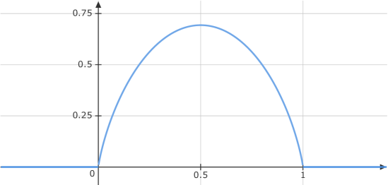
Figure 1. Plot of the function $\eta$. Note that it is non-differentiable at $x=0$ and $x=1$, but smooth everywhere else. Moreover, it vanishes at $x=0$ and $x=1$.

For the entanglement entropy we need to assume that the Hilbert space $\mathscr{H}_{m}$ is formed of wave functions in spacetime. Restricting them to a Cauchy surface, we obtain functions defined on three-dimensional space $\mycal N$ (which could be $\mathbb{R}^{3}$ or, more generally, a three-dimensional manifold). Given a spatial subregion $\Lambda\subset\mycal N$, the entanglement entropy $H(\Omega,\Lambda)$ is defined by (for details see [17, Section 3])

$$H(\Pi_{\varepsilon}^{-},\Lambda):=\operatorname{tr}\Delta(\Omega,\Lambda)+\operatorname{tr}\Delta(\Pi_{\varepsilon}^{-},\mycal N\setminus\Lambda)\>,$$

where $\Delta(\Pi_{\varepsilon}\varepsilon^{-},\Lambda)$ is the entropic difference operator

$$\Delta(\Pi_{\varepsilon}^{-},\Lambda):=\eta\big{(}\chi_{\Lambda}\,\Pi_{\varepsilon}^{-}\,\chi_{\Lambda}\big{)}-\big{(}\chi_{\Lambda}\,\eta(\Pi_{\varepsilon}^{-})\,\chi_{\Lambda}\big{)}\>.$$

Note that here and in the rest of the paper we sometimes identify the multiplication operator $\mathcal{M}_{f}$ by the function $f$ with the corresponding function. For example we just used this convention when writing $\chi_{\Lambda}\Pi_{\varepsilon}^{-}\chi_{\Lambda}$ for $\mathcal{M}_{\chi_{\Lambda}}\Pi_{\varepsilon}^{-}\mathcal{M}_{\chi_{\Lambda}}$.

Remark 2.1.

We point out that our definition of entanglement entropy differs from the conventions in [15, 17] in that we do not add the entropic difference operator of the complement of $\tilde{\Lambda}$. This is justified as follows. On the technical level, our procedure is easier, because it suffices to consider compact spatial regions (indeed, we expect that the entropic difference operator on the complement of $\tilde{\Lambda}$ is not trace class). Conceptually, restricting attention to the entropic difference operator of $\tilde{\Lambda}$ can be understood from the fact that occupied states which are supported either inside or outside $\tilde{\Lambda}$ do not contribute to the entanglement entropy. Thus it suffices to consider the states which are non-zero both inside and outside. These “boundary states” are taken into account already in the entropic difference operator (1.1).

This qualitative argument can be made more precise with the following formal computation, which shows that at least the unregularized entropic difference is the same for the inner and the outer parts: First of all note that $\eta(x)$ vanishes at $x=0$ and $x=1$. Since $\Pi^{-}$ is a projection this means that

$$\eta(\Pi^{-})=0\qquad\text{and therefore}\qquad\operatorname{tr}\big{(}\chi_{\tilde{\Lambda}}\>\eta(\Pi^{-})\>\chi_{\tilde{\Lambda}}\big{)}=0=\operatorname{tr}\big{(}\chi_{\tilde{\Lambda}^{c}}\>\eta(\Pi^{-})\>\chi_{\tilde{\Lambda}^{c}}\big{)}\>.$$

Moreover, if we assume that both $\chi_{\tilde{\Lambda}}\>\Pi^{-}\>\chi_{\tilde{\Lambda}}$ and $\Pi^{-}\>\chi_{\tilde{\Lambda}}\>\Pi^{-}$ are compact operators, we can find a one-to-one correspondence between their non-zero eigenvalues: Take any eigenvector $\psi$ of $\chi_{\tilde{\Lambda}}\>\Pi^{-}\>\chi_{\tilde{\Lambda}}$ with eigenvalue $\lambda\neq 0$, then we must have

$$\chi_{\tilde{\Lambda}}\psi=\frac{1}{\lambda}\chi_{\tilde{\Lambda}}^{2}\>\Pi^{-}\>\chi_{\tilde{\Lambda}}\psi=\psi\qquad\text{and}\qquad\Pi^{-}\psi\neq 0\>,$$

which yields

$$\lambda\>\psi=\big{(}\chi_{\tilde{\Lambda}}\>\Pi^{-}\>\chi_{\tilde{\Lambda}}\big{)}\psi=\big{(}\chi_{\tilde{\Lambda}}\>\Pi^{-}\big{)}\psi\>.$$

Then $\Pi^{-}\psi$ is an eigenvector of $\Pi^{-}\>\chi_{\tilde{\Lambda}}\>\Pi^{-}$ with eigenvalue $\lambda$ because

$$\big{(}\Pi^{-}\>\chi_{\tilde{\Lambda}}\>\Pi^{-}\big{)}(\Pi^{-}\psi)=\Pi^{-}\big{(}\chi_{\tilde{\Lambda}}\>\Pi^{-}\big{)}\psi=\lambda\>\Pi^{-}\psi\>.$$

Since the same argument also works with the roles of $\Pi^{-}\>\chi_{\tilde{\Lambda}}\>\Pi^{-}$ and $\chi_{\tilde{\Lambda}}\>\Pi^{-}\>\chi_{\tilde{\Lambda}}$ interchanged, this shows, that the nonzero eigenvalues of both operators (counted with multiplicities) coincide. Then the same holds true for $\eta(\Pi^{-}\>\chi_{\tilde{\Lambda}}\>\Pi^{-})$ and $\eta(\chi_{\tilde{\Lambda}}\>\Pi^{-}\>\chi_{\tilde{\Lambda}})$, proving that

$$\operatorname{tr}\eta(\chi_{\tilde{\Lambda}}\>\Pi^{-}\>\chi_{\tilde{\Lambda}})=\operatorname{tr}\eta(\Pi^{-}\>\chi_{\tilde{\Lambda}}\>\Pi^{-})\>.$$

Due to the symmetry of $\eta$, namely

$$\eta(x)=\eta(1-x)\qquad\text{for any }x\in\mathbb{R}\>,$$

this then leads to

$$\operatorname{tr}\eta(\chi_{\tilde{\Lambda}}\>\Pi^{-}\>\chi_{\tilde{\Lambda}})=\operatorname{tr}\eta(\Pi^{-}\>\chi_{\tilde{\Lambda}}\>\Pi^{-})=\operatorname{tr}\eta\big{(}\Pi^{-}-\Pi^{-}\>\chi_{\tilde{\Lambda}}\>\Pi^{-}\big{)}=\operatorname{tr}\eta(\Pi^{-}\>\chi_{\tilde{\Lambda}^{c}}\>\Pi^{-})\>.$$

Repeating the same argument as before with $\chi_{\tilde{\Lambda}^{c}}\>\Pi^{-}\>\chi_{\tilde{\Lambda}^{c}}$ finally gives

$$\operatorname{tr}\eta(\chi_{\tilde{\Lambda}}\>\Pi^{-}\>\chi_{\tilde{\Lambda}})=\operatorname{tr}\eta(\Pi^{-}\>\chi_{\tilde{\Lambda}}\>\Pi^{-})=\operatorname{tr}\eta\big{(}\Pi^{-}-\Pi^{-}\>\chi_{\tilde{\Lambda}}\>\Pi^{-}\big{)}=\operatorname{tr}\eta(\Pi^{-}\>\chi_{\tilde{\Lambda}^{c}}\>\Pi^{-})$$

$$=\operatorname{tr}\eta(\chi_{\tilde{\Lambda}^{c}}\>\Pi^{-}\>\chi_{\tilde{\Lambda}^{c}})\>.$$

As a consequence, the corresponding entanglement entropy is given by

$$H(\Pi_{\varepsilon}^{-},\tilde{\Lambda}):=\Delta(\Pi_{\varepsilon}^{-},\tilde{\Lambda})+\Delta(\Pi_{\varepsilon}^{-},\tilde{\Lambda}^{c})=2\Big{(}\operatorname{tr}\eta\big{(}\chi_{\tilde{\Lambda}}\>\Pi^{-}\>\chi_{\tilde{\Lambda}}\big{)}-\chi_{\tilde{\Lambda}}\>\operatorname{tr}\eta(\Pi^{-})\>\chi_{\tilde{\Lambda}}\Big{)}\>.$$

Regularizing this expression, we end up with twice the entropic difference with respect to $\Pi^{-}_{\varepsilon}$ and $\tilde{\Lambda}$.   $\Diamond$

2.2. The Dirac Equation in Globally Hyperbolic Spacetimes

Since we are ultimately interested in Schwarzschild space time, the abstract setting for the Dirac equation is given as follows (for more details see for example [8]). Our starting point is a four dimensional, smooth, globally hyperbolic Lorentzian spin manifold $(\mycal M,g)$, with metric $g$ of signature $(+,-,-,-)$. We denote the corresponding spinor bundle by $S\mycal M$. Its fibres $S_{x}\mycal M$ are endowed with an inner product $\mbox{$\prec\!\!$ \nolinebreak}.|.\mbox{\nolinebreak$\succ$}_{x}$ of signature $(2,2)$, referred to as the spin inner product. Moreover, the mapping

$$\gamma\>:\>T_{x}\mycal M\rightarrow\text{\rm{L}}(S_{x}\mycal M)\>,\quad u\mapsto\sum\nolimits_{j=0}^{3}\gamma^{j}u_{j}\>,$$

where the $\gamma^{j}$ are the Dirac matrices defined via the anti-commutation relations

$$\gamma(u)\,\gamma(v)+\gamma(v)\,\gamma(u)=2\,g(u,v)\,\mbox{\rm 1 1}_{S_{x}(\mycal M)}\>,$$

provides the structure of a Clifford multiplication.

Smooth sections in the spinor bundle are denoted by $C^{\infty}(\mycal M,S\mycal M)$. Likewise, $C^{\infty}_{0}(\mycal M,S\mycal M)$ are the smooth sections with compact support. We also refer to sections in the spinor bundle as wave functions. The Dirac operator ${\mathcal{D}}$ takes the form

$${\mathcal{D}}:=i\gamma^{j}\nabla_{j}\>:\>C^{\infty}(\mycal M,S\mycal M)\rightarrow C^{\infty}(\mycal M,S\mycal M)\>,$$

where $\nabla$ denotes the connections on the tangent bundle and the spinor bundle. Then the Dirac equation with parameter $m$ (in the physical context corresponding to the particle mass) reads

$$({\mathcal{D}}-m)\,\psi=0\>.$$

Due to global hyperbolicity, our spacetime admits a foliation by Cauchy surfaces $\mycal M=(\mycal N_{t})_{t\in\mathbb{R}}$. Smooth initial data on any such Cauchy surface yield a unique global solution of the Dirac equation. Our main focus lies on smooth solutions with spatially compact support, denoted by $C^{\infty}_{\rm{sc}}(\mycal M,S\mycal M)$. The solutions in this class are endowed with the scalar product

$$(\psi|\phi)_{m}=\int N\mbox{$\prec\!\!$ \nolinebreak}\psi\,|\,\nu^{j}\gamma_{j}\,\phi\mbox{\nolinebreak$\succ$}_{x}\>d\mu N(x)\>,$$

where $\mycal N$ is a Cauchy surface $\mycal N$ with future-directed normal $\nu$ (compared to the conventions in [8], we here preferred to leave out a factor of $2\pi$). This scalar product is independent on the choice of $\mycal N$ (for details see [8, Section 2]). Finally we define the Hilbert space $(\mathscr{H}_{m},(.|.)_{m})$ by completion,

$$\mathscr{H}_{m}:=\overline{C^{\infty}_{\rm{sc}}(\mycal M,S\mycal M)}^{(.|.)_{m}}\>.$$

2.3. The Dirac Propagator in the Schwarzschild Geometry

2.3.1. The Integral Representation of the Propagator

We recall the form of the Dirac equation in the Schwarzschild geometry and its separation, closely following the presentation in [7] and [9]. Given a parameter $M>0$ (the black hole mass), the exterior Schwarzschild metric reads

$$ds^{2}=g_{jk}\>dx^{j}\,dx^{k}=\frac{\Delta(r)}{r^{2}}\>dt^{2}-\frac{r^{2}}{\Delta}\>dr^{2}-r^{2}\>d\vartheta^{2}-r^{2}\>\sin^{2}\vartheta\>d\varphi^{2}\>,$$

where

$$\Delta(r):=r^{2}-2Mr\>.$$

Here the coordinates $(t,r,\vartheta,\varphi)$ takes values in the intervals

$$-\infty<t<\infty,\qquad r_{1}<r<\infty,\qquad 0<\vartheta<\pi,\qquad 0<\varphi<2\pi\>,$$

where $r_{1}:=2M$ is the event horizon.

In this geometry, the Dirac operator takes the form (see also [9, Section 2.2]):

$${\mathcal{D}} =\begin{pmatrix}0&0&\alpha_{+}&\beta_{+}\\ 0&0&\beta_{-}&\alpha_{-}\\ \alpha_{-}&-\beta_{+}&0&0\\ -\beta_{-}&\alpha_{+}&0&0\end{pmatrix}\qquad\text{with}$$

$$\beta_{\pm} =\frac{i}{r}\left(\frac{\partial}{\partial\vartheta}+\frac{\cot\vartheta}{2}\right)\pm\frac{1}{r\sin\vartheta}\>\frac{\partial}{\partial\varphi}\qquad\text{and}$$

$$\alpha_{\pm} =-\frac{ir}{\sqrt{\Delta}}\>\frac{\partial}{\partial t}\pm\frac{\sqrt{\Delta}}{r}\left(i\frac{\partial}{\partial r}\>+\>i\>\frac{r-M}{2\Delta}\>+\>\frac{i}{2r}\right).$$

It is most convenient to transform the radial coordinate to the so called Regge-Wheeler-coordinate $u\in\mathbb{R}$ defined by

$$u(r)=r+2M\log(r-2M)\>,\qquad\text{so that}\qquad\frac{du}{dr}=\frac{r^{2}}{\Delta}\>.$$

In this coordinate, the event horizon is located at $u\rightarrow-\infty$, whereas $u\rightarrow\infty$ corresponds to spatial infinity i.e. $r\rightarrow\infty$. Then the Dirac equation can be separated with the ansatz

$$\psi^{kn\omega}(t,u,\varphi,\vartheta)=e^{-ik\varphi}\>\frac{1}{\Delta^{1/4}\sqrt{r}}\>\begin{pmatrix}X_{-}^{kn}(t,u)Y^{kn}_{-}(\vartheta)\\ X_{+}^{kn}(t,u)Y^{kn}_{+}(\vartheta)\\ X_{+}^{kn}(t,u)Y^{kn}_{-}(\vartheta)\\ X_{-}^{kn}(t,u)Y^{kn}_{+}(\vartheta)\end{pmatrix}$$

with $k\in\mathbb{Z}+1/2$, $n\in\mathbb{N}$ and $\omega\in\mathbb{R}$. The angular functions $Y^{kn}_{\pm}$ can be expressed in terms of spin-weighted spherical harmonics. The radial functions $X^{kn}_{\pm}$ satisfy a system of partial differential equations

$$\begin{pmatrix}\sqrt{\Delta}\mathcal{D}_{+}&imr-\lambda\\ -imr-\lambda&\sqrt{\Delta}\mathcal{D}_{-}\end{pmatrix}\begin{pmatrix}X_{+}^{kn}\\ X_{-}^{kn}\end{pmatrix}=0\>,$$ (2.2)

where

$$\mathcal{D}_{\pm}=\frac{\partial}{\partial r}\mp\frac{r^{2}}{\Delta}\>\frac{\partial}{\partial t}\>,$$

for details see [7, Section 2]. Moreover, employing the ansatz

$$X^{kn}_{\pm}(t,u)=e^{-i\omega t}\>X^{kn\omega}_{\pm}(u)\>,$$

equation (2.2) goes over to a system of ordinary differential equations, which admits two two-component fundamental solutions labeled by $a=1,2$. We denote the resulting Dirac solution by $X^{kn\omega}_{a}=(X^{kn\omega}_{a,+},X^{kn\omega}_{a,-})$ (for more details on the choice of the fundamental solutions see Section 2.3.4 below).

In what follows we will often use the following notation for two-component functions

$$A:=\begin{pmatrix}A_{+}\\ A_{-}\end{pmatrix}\>.$$

The norm in $\mathbb{C}^{2}$ will be denoted by $|\,.\,|$, the canonical inner product on $L^{2}(\mathbb{R},\mathbb{C}^{2})$ by $\langle.|.\rangle$ and the corresponding norm by $\|.\|$.

As implied by [7, Theorem 3.6], one can then find the following formula for the mode-wise propagator:

Theorem 2.2.

Given initial radial data $X_{0}\in C^{\infty}_{0}(\mathbb{R},\mathbb{C}^{2})$ at time $t=0$, the corresponding solution $\psi\in C^{\infty}_{0}(\mathbb{R}^{2},\mathbb{C}^{2})$ of the radial Dirac equation (2.2) can be written as

$$X(t,u)=\frac{1}{\pi}\int_{-\infty}^{\infty}d\omega\>e^{-i\omega t}\sum_{a,b=1}^{2}t_{ab}^{kn\omega}\,X_{a}^{kn\omega}(u)\>\langle X_{b}^{kn\omega}|X_{0}\rangle_{L^{2}}\>,$$

for any $u,t\in\mathbb{R}$. The $X_{a}^{kn\omega}(x)$ are the fundamental solutions mentioned before. Here the coefficients $t_{ab}^{kn\omega}$ satisfy the relations

$$\overline{t^{kn\omega}_{ab}}=t^{kn\omega}_{ba}$$

and

$$\left\{\begin{array}[]{cl}t^{kn\omega}_{ab}=\delta_{a,1}\>\delta_{b,1}&\qquad\text{if~{}$|\omega|\leq m$}\\[3.00003pt] \displaystyle t^{kn\omega}_{11}=t_{22}=\frac{1}{2}\>,\quad\big{|}t^{kn\omega}_{12}\big{|}\leq\frac{1}{2}&\qquad\text{if~{}$|\omega|>m$}\>.\end{array}\right.$$ (2.3)

2.3.2. Hamiltonian Formulation

We may rewrite the Dirac equation in Hamilton form, i.e.

$$i\frac{\partial}{\partial t}X^{kn}(t,u)=\big{(}H_{kn}X^{kn}|_{t}\big{)}(u)$$

$$\Longleftrightarrow\qquad ({\mathcal{D}}-m)\,e^{-ik\varphi}\>\frac{1}{\Delta^{1/4}\sqrt{r}}\>\begin{pmatrix}X^{kn}_{-}(t,u)Y^{kn}_{-}(\vartheta)\\ X^{kn}_{+}(t,u)Y^{kn}_{+}(\vartheta)\\ X^{kn}_{+}(t,u)Y^{kn}_{-}(\vartheta)\\ X^{kn}_{-}(t,u)Y^{kn}_{+}(\vartheta)\end{pmatrix}=0\;,$$

where the Hamiltonian $H_{kn}$ is an essentially self-adjoint operator on $L^{2}(\mathbb{R},\mathbb{C}^{2})$ with dense domain $\mathscr{D}(H)=C^{\infty}_{0}(\mathbb{R},\mathbb{C}^{2})$. This makes it possible to write the solution of the Cauchy problem as

$$X(t,u)=\big{(}e^{-itH_{kn}}\,X_{0}\big{)}(u)\qquad\text{with~{}$u\in\mathbb{R}$}\>.$$

Here, the initial data can be an arbitrary vector-valued function in the Hilbert space, i.e. $X_{0}\in L^{2}(\mathbb{R},\mathbb{C}^{2})$. If we specialize to smooth initial data with compact support, i.e. $X_{0}\in C^{\infty}_{0}(\mathbb{R},\mathbb{C}^{2})$, then the time evolution operator can be written with the help of Theorem 2.2 as

$$\big{(}e^{-itH_{kn}}X_{0}\big{)}(u)=\frac{1}{\pi}\int_{-\infty}^{\infty}d\omega\>e^{-i\omega t}\sum_{a,b=1}^{2}t_{ab}^{kn\omega} \,X_{a}^{kn\omega}(u)\>\langle X_{b}^{kn\omega}|X_{0}\rangle$$

for $$X_{0}\in C^{\infty}_{0}(\mathbb{R},\mathbb{C}^{2})$$

We point out that this formula does not immediately extend to general $X_{0}\in L^{2}(\mathbb{R},\mathbb{C}^{2})$; we will come back to this technical issue a few times in this paper.

2.3.3. Connection to the Full Propagator

In this section we will explain, why it suffices to focus on one angular mode instead of the full propagator and why we can use the ordinary $L^{2}$-scalar product instead of $(.|.)_{m}$.

To this end, we introduce the function

$$S:=\Delta^{1/4}\sqrt{r}\>.$$

Moreover, for each fixed $k\in\mathbb{Z}+1/2$, $n\in\mathbb{Z}$ we denote by $(\mathscr{H}_{m}^{0})_{kn}$ the completion of

$$V_{kn}:=\mathrm{span}\bigg{\{}S^{-1}\>e^{-ik\varphi}\>\begin{pmatrix}X^{kn\omega}_{-}(u)Y^{kn}_{-}(\vartheta)\\ X^{kn\omega}_{+}(u)Y^{kn}_{+}(\vartheta)\\ X^{kn\omega}_{+}(u)Y^{kn}_{-}(\vartheta)\\ X^{kn\omega}_{-}(u)Y^{kn}_{+}(\vartheta)\end{pmatrix}\>\bigg{|}\>X=(X_{+},X_{-})\in L^{2}(\mathbb{R},\mathbb{C}^{2})\bigg{\}}\>,$$

with respect to $(.|.)_{m}$, i.e.

$$(\mathscr{H}_{m}^{0})_{kn}:=\overline{V_{kn}}^{(.|.)_{m}}\>.$$

This space can be thought of as the mode-wise solution space of the Dirac-equation at time $t=0$. Note that the entire Hilbert space of solutions at time $t=0$, namely

$$\mathscr{H}_{m}|_{t=0}=:\mathscr{H}_{m}^{0}$$

has the orthogonal decomposition

$$\mathscr{H}_{m}^{0}=\bigoplus_{i\in\mathbb{N}}(\mathscr{H}_{m}^{0})_{k_{i}n_{i}}\>.$$ (2.4)

(again with respect to $(.|.)_{m}$), where $((k_{i},n_{i}))_{i\in\mathbb{N}}$ is an enumeration of $(\mathbb{Z}+1/2)\times\mathbb{Z}$. Furthermore, each space $(\mathscr{H}_{m}^{0})_{kn}$ can be connected with $L^{2}(\mathbb{R},\mathbb{C}^{2})$ using the mapping

$$\tilde{S}:\big{(}(\mathscr{H}_{m}^{0})_{kn}\>,\>(.|.)_{m}\big{)}\rightarrow L^{2}(\mathbb{R},\mathbb{C}^{2})\>,$$

$$\psi\mapsto S\>\begin{pmatrix}\displaystyle\;\int\Big{\langle}\big{(}\psi_{2}\,,\,\psi_{3}\big{)}\>\Big{|}\>e^{-ik\varphi}\>\big{(}Y^{kn}_{+}(\vartheta)\>,\>Y^{kn}_{-}(\vartheta)\big{)}\Big{\rangle}_{\mathbb{C}^{2}}d\Omega\vspace{0.1cm}\\ \displaystyle\;\int\Big{\langle}\big{(}\psi_{1}\,,\,\psi_{4}\big{)}\>\Big{|}\>e^{-ik\varphi}\>\big{(}Y^{kn}_{+}(\vartheta)\>,\>Y^{kn}_{-}(\vartheta)\big{)}\Big{\rangle}_{\mathbb{C}^{2}}d\Omega\end{pmatrix}\>,$$

with inverse

$$\tilde{S}^{-1}:L^{2}(\mathbb{R},\mathbb{C}^{2}) \rightarrow\big{(}(\mathscr{H}_{m}^{0})_{kn}\>,\>(.|.)_{m}\big{)}\>,$$

$$(X_{+},X_{-}) \mapsto S^{-1}e^{-ik\varphi}\begin{pmatrix}X_{-}(u)Y^{kn}_{-}(\vartheta)\\ X_{+}(u)Y^{kn}_{+}(\vartheta)\\ X_{+}(u)Y^{kn}_{-}(\vartheta)\\ X_{-}(u)Y^{kn}_{+}(\vartheta)\end{pmatrix}\>.$$

Then a direct computation shows the scalar products transform as

$$\langle\tilde{S}\psi\>|\>\tilde{S}\phi\rangle_{L^{2}}=(\psi\,|\,\phi)_{m}\qquad\text{for any }\phi,\psi\in(\mathscr{H}_{m}^{0})_{kn}\>.$$

This shows that $\tilde{S}$ is unitary and we can identify the two spaces.

Now recall that the Dirac-equation can be separated by solutions of the form

$$\hat{\psi}=S^{-1}e^{-ik\varphi}\begin{pmatrix}X_{-}(t,u)Y^{kn}_{-}(\vartheta)\\ X_{+}(t,u)Y^{kn}_{+}(\vartheta)\\ X_{+}(t,u)Y^{kn}_{-}(\vartheta)\\ X_{-}(t,u)Y^{kn}_{+}(\vartheta)\end{pmatrix}\>,$$

and can then be described mode-wise by the Hamiltonian $H_{kn}$ on the space $L^{2}(\mathbb{R},\mathbb{C}^{2})$. Therefore denoting

$$\tilde{H}_{kn}:=\tilde{S}^{-1}H_{kn}\tilde{S}\>,$$

the diagonal block operator (with respect to the decomposition (2.4))

$$\tilde{H}:=\text{diag}\big{(}\tilde{H}_{(k_{1},n_{1})}\>,\>\tilde{H}_{(k_{2},n_{2})}\>,\>\dots\>\big{)}\>,$$

defines an essentially self-adjoint Hamiltonian for the original Dirac equation on the space $\mathscr{H}_{m}^{0}$.

Moreover, any function of $\tilde{H}$ is of the same diagonal block operator form. The same holds for any multiplication operator $\mathcal{M}_{\chi_{\tilde{U}}}$, where $\tilde{U}$ is a spherical symmetric set

$$\tilde{U}:=U\times S^{2}\subseteq\mathbb{R}\times S^{2}\>.$$

In particular, such an operator has the block operator representation

$$\mathcal{M}_{\chi_{\tilde{U}}}=\text{diag}\big{(}\mathcal{M}_{\chi_{\tilde{U}}}\>,\>\mathcal{M}_{\chi_{\tilde{U}}}\>,\>\dots\big{)}\>.$$

We therefore conclude that when computing traces of operators of the form

$$\chi_{\tilde{U}}f(\tilde{H})\chi_{\tilde{U}}\qquad\text{or}\qquad f(\chi_{\tilde{U}}\tilde{H}\chi_{\tilde{U}})\>,$$

(for some suitable function $f$), we may consider each angular mode separately and then sum over the occupied states (and similarly for Schatten norms of such operators).

Moreover we point out that instead of $(\mathscr{H}_{m}^{0})_{kn}$ we can work with the corresponding objects in $L^{2}(\mathbb{R},\mathbb{C}^{2})$, as the spaces are unitarily equivalent. Note, that then the multiplication operator $\mathcal{M}_{\chi_{\tilde{U}}}$ goes over to $\mathcal{M}_{\chi_{U}}$, i.e.

$$\tilde{S}^{-1}\mathcal{M}_{\chi_{\tilde{U}}}\tilde{S}=\mathcal{M}_{\chi_{U}}\>.$$

In particular this leads to

$$\operatorname{tr}\Big{(}\chi_{\tilde{U}}f(\tilde{H})\chi_{\tilde{U}}\Big{)}=\>\sum_{\mathclap{\begin{subarray}{c}(k,n)\\ \text{occupied}\end{subarray}}}\>\operatorname{tr}\Big{(}\chi_{\tilde{U}}f(\tilde{H}_{kn})\chi_{\tilde{U}}\Big{)}=\>\sum_{\mathclap{\begin{subarray}{c}(k,n)\\ \text{occupied}\end{subarray}}}\>\operatorname{tr}\Big{(}\chi_{U}f(H_{kn})\chi_{U}\Big{)}$$

and

$$\operatorname{tr}f\big{(}\chi_{\tilde{U}}\tilde{H}\chi_{\tilde{U}}\big{)}=\>\sum_{\mathclap{\begin{subarray}{c}(k,n)\\ \text{occupied}\end{subarray}}}\>\operatorname{tr}f\big{(}\chi_{\tilde{U}}\tilde{H}_{kn}\chi_{\tilde{U}}\big{)}=\>\sum_{\mathclap{\begin{subarray}{c}(k,n)\\ \text{occupied}\end{subarray}}}\>\operatorname{tr}f\big{(}\chi_{U}H_{kn}\chi_{U}\big{)}\>.$$

2.3.4. Asymptotics of the Radial Solutions

We now recall the asymptotics of the solutions of the radial ODEs and specify our choice of fundamental solutions. Since we want to consider the propagator at the horizon, we will need near-horizon approximations of the $X^{kn\omega}$’s. In order to control the resulting error terms, we now state a slightly stronger version of [7, Lemma 3.1], specialized to the Schwarzschild case.

Lemma 2.3.

For any $u_{2}\in\mathbb{R}$ fixed, in Schwarzschild space every solution $X\equiv X^{kn\omega}$ for $u\in(-\infty,u_{2})$ is of the form

$$X(u)=\begin{pmatrix}f_{0}^{+}e^{-i\omega u}\\ f_{0}^{-}e^{i\omega u}\end{pmatrix}+R_{0}(u)$$

where the error term $R_{0}$ decays exponentially in $u$, uniformly in $\omega$. More precisely, writing

$$R_{0}(u)=\begin{pmatrix}e^{-i\omega u}g^{+}(u)\\ e^{i\omega u}g^{-}(u)\end{pmatrix}\>,$$

the vector-valued function $g=(g^{+},g^{-})$ satisfies the bounds

$$|g(u)|<ce^{du}\>,\quad\left|\frac{d}{du}g(u)\right|\leq dce^{du}\qquad\mathrm{for\;all\;}u<u_{2}\>,$$

with coefficients

$$d=\frac{1}{M}\>,\quad c=\sqrt{\frac{M}{2e}}\Big{(}m+\frac{|\lambda|}{2M}\Big{)}|f_{0}|\exp\bigg{(}8\sqrt{\frac{M}{2e}}\Big{(}m+\frac{|\lambda|}{2M}\Big{)}e^{u_{2}/M}\bigg{)}\>,$$

where $\lambda$ is a dimensionless constant depending only on $k$ and $n$.

The proof, which follows the method in [7], is given in detail in Appendix A.

We can now explain how to construct the fundamental solutions $X_{a}=(X_{a}^{+},X_{a}^{-})$ for $a=1$ and $2$ (for this see also [7, p. 41] and [9, p. 9-10]). In the case $|\omega|>m$ we choose $X_{1}$ and $X_{2}$ such that the corresponding functions $f_{0}$ from the previous lemma are of the form

$$f_{0}=\begin{pmatrix}1\\ 0\end{pmatrix}\;\mathrm{for\;}X_{1}\qquad\text{and}\qquad f_{0}=\begin{pmatrix}0\\ 1\end{pmatrix}\;\mathrm{for\;}X_{2}\>.$$

In the case $|\omega|\leq m$ we consider the behavior of solutions at infinity (i.e. asymptotically as $u\rightarrow\infty$). It turns out that there is (up to a prefactor) a unique fundamental solution which decays exponentially. We denote it by $X_{1}$. Moreover, we choose $X_{2}$ as an exponentially increasing fundamental solution. We normalize the resulting fundamental system at the horizon by

$$\lim\limits_{u\rightarrow-\infty}|X_{1/2}|=1\>.$$

Representing these solutions in the form of the previous lemma we obtain

$$X_{1/2}(u)=\begin{pmatrix}e^{-i\omega u}f^{+}_{0,1/2}\\ e^{i\omega u}f^{-}_{0,1/2}\end{pmatrix}+R_{0,1/2}(u)$$

with coefficients $f_{0,1/2}^{\pm}\in\mathbb{C}$. Due to the normalization, we know that

$$|f_{0,1/2}|=1\qquad\text{and in particular}\qquad|f_{0,1/2}^{\pm}|\leq 1\>.$$

Note however, that $f_{0}$ and $R_{0}$ from the previous Lemma may in general also depend on $k$ and $n$, but we will suppress to corresponding indices for ease of notation.

2.4. Schatten Classes and Norms

As we will later see, we can often estimate traces of functions of operators by their so called Schatten norms, which we now introduce (the following definition and example are based on [26, Section 2.1]).

Definition 2.4.

Let $\mathfrak{H}$ and $\mathfrak{G}$ be Hilbert spaces and $\mathfrak{S}_{\infty}$ the set of compact operators from $\mathfrak{H}$ to $\mathfrak{G}$. Moreover, let $\mathfrak{S}\subseteq\mathfrak{S}_{\infty}$ be a two-sided ideal with a functional $\|.\|_{\mathfrak{S}}$ on it, then $\|.\|_{\mathfrak{S}}$ is called a quasi-norm if the following three conditions are satisfied

• $\|T\|_{\mathfrak{S}}>0$ for all nonzero $T\in\mathfrak{S}$

• $\|zT\|_{\mathfrak{S}}=|z|\|T\|_{\mathfrak{S}}$ for all $z\in\mathbb{C}$ and $T\in\mathfrak{S}$

• There is a $\kappa\geq 1$ with

  $$\|T_{1}+T_{2}\|_{\mathfrak{S}}\leq\kappa(\|T_{1}\|_{\mathfrak{S}}+\|T_{2}\|_{\mathfrak{S}})\>,$$

  for any $T_{1},T_{2}\in\mathfrak{S}$.

Moreover, if a quasi-norm $\|.\|_{\mathfrak{S}}$ is called symmetric if it fulfills the two additional conditions

• $\|XTY\|_{\mathfrak{S}}\leq\|X\|_{\infty}\|Y\|_{\infty}\|T\|_{\mathfrak{S}}$ for all $T\in\mathfrak{S}$ and $X,Y$ bounded with $\|.\|_{\infty}$ denoting the operator norm (throughout the paper)

• $\|T\|_{\mathfrak{S}}=\|T\|_{\infty}$ for any $T\in\mathfrak{S}$ with one-dimensional image.

Let $\mathfrak{S}$ as before with a symmetric quasi-norm $\|.\|_{\mathfrak{S}}$ such that $\mathfrak{S}$ is complete, then the pair $(\mathfrak{S},\|.\|_{\mathfrak{S}})$ is referred to as a quasi-normed ideal.

A quasi-normed ideal $(\mathfrak{S},\|.\|_{\mathfrak{S}})$ is called q-normed ideal if there is an equivalent quasi-norm $\operatorname{|||}.\operatorname{|||}_{\mathfrak{S}}$ such that the so called $q$-triangle-inequality

$$\operatorname{|||}T_{1}+T_{2}\operatorname{|||}_{\mathfrak{S}}^{q}\leq\operatorname{|||}T_{1}\operatorname{|||}_{\mathfrak{S}}^{q}+\operatorname{|||}T_{2}\operatorname{|||}_{\mathfrak{S}}^{q}\>,\quad\mathrm{for\;all\;}T_{1},T_{2}\in\mathfrak{S}\>,$$

is fulfilled.

In what follows we will sometimes use the convention, that if we write $\|T\|_{\mathfrak{S}}$ for any operator $T\in\text{\rm{L}}(\mathfrak{H},\mathfrak{G})$ then we automatically imply that $T$ is already in $\mathfrak{S}$.

Example 2.5.

Let $q\in(0,\infty)$ and $\mathfrak{S}_{q}$ be the $q^{\text{th}}$ Schatten-von-Neumann ideal, i.e. all compact operators $T$ such that

$$\|T\|_{q}:=\left[\sum_{k=1}^{\infty}s_{k}(T)^{q}\right]^{1/q}$$

is finite, where the $s_{k}(T)$ denote the singular numbers of $T$, i.e. the square roots of the eigenvalues of $T^{*}T$ (which are clearly non-negative). Then for $q\geq 1$ the functional $\|.\|_{q}$ defines a norm and for $q\in(0,1)$ a $q$-norm (see [26, Section 2.1] with references to [5] and [21]).

Note that for $q=1$ this coincides with the trace-norm.   $\Diamond$

Remark 2.6.

Note that the $q$-th Schatten-norm is invariant under unitary transformations: Let $\mathfrak{H}$ and $\mathfrak{G}$ be Hilbert spaces, $U\in\text{\rm{L}}(\mathfrak{G},\mathfrak{H})$ unitary and $A\in\mathfrak{S}^{q}\subseteq\text{\rm{L}}(\mathfrak{H})$ then

$$(U^{-1}AU)^{*}U^{-1}AU=(U^{*}AU)^{*}U^{-1}AU=U^{*}A^{*}UU^{-1}AU=U^{-1}A^{*}AU\;,$$

which is unitarily equivalent to $A^{*}A$ and thus has the same eigenvalues showing that

$$\|A\|_{q}=\|U^{-1}AU\|_{q}\>.$$

In particular, in the case $q=1$ this shows that the trace norm of $A$ is conserved under unitary transformation.

Moreover, we will frequently use the following function norms (see for example [24, p. 5-6] with slight modifications)

Definition 2.7.

Let $S^{(n,m,k)}(\mathbb{R}^{d})$ with $m,n,k\in\mathbb{N}_{0}$ be the space of all complex-valued functions on $(\mathbb{R}^{d})^{3}$, which are continuous, bounded and continuously partially differentiable in the first variable up to order $n$, in the second to $m$ and in the third to $k$ and whose partial derivatives up to these orders are bounded as well. For $b\in S^{(n,m,k)}$ and $l,r>0$ we introduce the norm

$$N^{(n,m,k)}(b;l,r):=\max_{\begin{subarray}{c}0\leq\tilde{n}\leq n\\ 0\leq\tilde{m}\leq m\\ 0\leq\tilde{k}\leq k\end{subarray}}\sup_{u,u^{\prime},\xi}l^{\tilde{n}+\tilde{m}}r^{\tilde{k}}\big{|}\nabla_{u}^{\tilde{n}}\nabla_{u^{\prime}}^{\tilde{m}}\nabla_{\xi}^{\tilde{k}}b(u,u^{\prime},\xi)\big{|}\>.$$

Similarly, $S^{(n,k)}(\mathbb{R}^{d})$ with $n,k\in\mathbb{N}_{0}$ denotes the space of all complex-valued functions on $(\mathbb{R}^{d})^{2}$, which are continuous and bounded and continuously partially differentiable in the first variable up to order $n$ and in the second to $m$ and whose partial derivatives up to these orders are bounded. For $b\in S^{(n,m)}(\mathbb{R}^{d})$ and $l,r>0$ we introduce the norm

$$N^{(n,k)}(b;l,r):=\max_{\begin{subarray}{c}0\leq\tilde{n}\leq n\\ 0\leq\tilde{k}\leq k\end{subarray}}\sup_{u,u^{\prime},\xi}l^{\tilde{n}}r^{\tilde{k}}\big{|}\nabla_{u}^{\tilde{n}}\nabla_{\xi}^{\tilde{k}}b(u,\xi)\big{|}\>.$$

Note that any symbol $b\in S^{(n,n)}$ may be interpreted as symbol in $\mathbb{R}^{d}$ by the identification

$$b(u,u^{\prime},\xi)\equiv b(u,\xi)\qquad\text{for any }u^{\prime}\in\mathbb{R}^{d}\>.$$

Then, for any $l,r>0$ and $m\in\mathbb{N}_{0}$ one has

$$N^{(n,m,k)}(b;l,r)=N^{(n,k)}(b;l,r)\>.$$

3. The Regularized Projection Operator

3.1. Definition and Basic Properties

As previously mentioned, the entropy is computed using the regularized projection operator to the negative frequency space $\Pi_{\varepsilon}^{-}$. This operator emerges from $e^{-itH_{kn}}$ from Section 2.3.2 by setting $t=i\varepsilon$ (the “$i\varepsilon$”-regularization) and restricting to the negative frequencies. Similar as explained in Section 2.3.3, for operators of this form it suffices to consider the corresponding operator for one angular mode $(\Pi_{\varepsilon}^{-})_{kn}$. So more precisely, for any $X\in C^{\infty}_{0}(\mathbb{R},\mathbb{C}^{2})$ the operator $(\Pi_{\varepsilon}^{-})_{kn}$ is defined by

$$\big{(}(\Pi_{\varepsilon}^{-})_{kn}\>X\big{)}(x):=\frac{1}{\pi}\int_{-\infty}^{0}d\omega\>e^{\varepsilon\omega}\sum_{a,b=1}^{2}t_{ab}^{kn\omega}X_{a}^{kn\omega}(x)\langle X_{b}^{kn\omega}|X\rangle\>,$$ (3.1)

for any $x\in\mathbb{R}$.

Since in this section we focus on one angular mode, we will drop the superscripts $kn$ on the functions $X^{kn\omega}_{a}$ and $t^{kn\omega}_{ab}$. Moreover, we will sometimes write the $\omega$-dependence of $X^{kn\omega}_{a}$ or $t^{kn\omega}_{ab}$ as an argument, i.e.

$$X^{kn\omega}_{a}(u)\equiv X^{\omega}_{a}(u)\equiv X_{a}(u,\omega)\qquad\textit{for any }u\in\mathbb{R}\>.$$

The asymptotics of the radial solutions at the horizon (Lemma 2.3) yield the following boundedness properties for the functions $X^{\omega}_{a}$:

Remark 3.1.

Given $u_{2}\in\mathbb{R}$ and a constant $C>0$, we consider measurable functions $X,Z:\mathbb{R}\rightarrow\mathbb{C}^{2}$ with the properties

$$\operatorname{supp}X,\>\operatorname{supp}Z\subset(-\infty,u_{2}]\qquad\text{and}\qquad\|X\|_{\infty},\|Z\|_{\infty}<C\>.$$

Then the estimate in Lemma 2.3 yields

$$\sum_{a,b}|t_{ab}^{\omega}|\>|X(u)|\>|X_{a}^{\omega}(u,\omega)|\>|X_{b}^{\omega}(u^{\prime},\omega)|\>|Z(u^{\prime})|\leq 2C^{2}\,(1+ce^{du})\,(1+ce^{du^{\prime}})\>,$$

for almost all $u,u^{\prime},\omega\in\mathbb{R}$ and with constants $c,d$ only depending on $k,n$ and $u_{2}$.

If we assume in addition that $\phi$ and $\psi$ are compactly supported, then for any $g\in L^{1}(\mathbb{R})$ the Lebesgue integral

$$\int_{-\infty}^{\infty}du\int_{-\infty}^{\infty}\frac{d\omega}{\pi}\>g(\omega)\int_{-\infty}^{\infty}du^{\prime}\>t_{ab}^{\omega}\>X^{\dagger}(u)\>X_{a}^{\omega}(u,\omega)\>X_{b}^{\omega}(u^{\prime},\omega)^{\dagger}\>Z(u^{\prime})\>,$$

is well-defined. Moreover, applying Fubini we may interchange the order of integration arbitrarily.

Furthermore, we will need the following technical Lemma, which tells us that testing with smooth and compactly supported functions suffices to determine if a function is in $L^{2}$ and to estimate its $L^{2}$-norm:

Lemma 3.2.

Let $N$ be a manifold with integration measure $\mu$. Given a function $f\in L^{1}_{\text{\rm{loc}}}(N,\mathbb{C}^{n})$ (with $n\in\mathbb{N}$), we assume that the corresponding functional on the test functions

$$\Phi\>:\>C^{\infty}_{0}(N,\mathbb{C}^{n})\rightarrow\mathbb{C}\>,\quad v\mapsto\int_{N}\langle v(x)\>|\>f(x)\rangle_{\mathbb{C}^{n}}\;d\mu(x)$$

is bounded with respect to the $L^{2}$-norm, i.e.

$$\big{|}\Phi(v)\big{|}\leq C\>\|v\|_{L^{2}(N,\mathbb{C}^{n})}\qquad\text{for all~{}$v\in C^{\infty}_{0}(N,\mathbb{C}^{n})$}\>.$$

Then $f\in L^{2}(N,\mathbb{C}^{n})$ and $\|f\|_{L^{2}(N,\mathbb{C}^{n})}\leq C$.

Proof.

Being bounded, the functional $\Phi$ can be extended continuously to $L^{2}(N,\mathbb{C}^{n})$. The Fréchet-Riesz theorem makes it possible to represent this functional by an $L^{2}$-function $\hat{f}$ i.e. $\|\hat{f}\|_{L^{2}(N,\mathbb{C}^{n})}\leq C$ and

$$\int_{N}\langle v(x),\big{(}f(x)-\hat{f}(x)\big{)}\rangle_{\mathbb{C}^{n}}\;d\mu(x)=0\qquad\text{for all~{}$v\in C^{\infty}_{0}(N,\mathbb{C}^{n})$}\>.$$

The fundamental lemma of the calculus of variations (for vector-valued functions on a manifold) yields that $f=\hat{f}$ almost everywhere. ∎

Now we have all the tools to prove the boundedness of the operator $(\Pi_{\varepsilon}^{-})_{kn}$.

Lemma 3.3.

Equation (3.1) defines a continuous endomorphism $(\Pi_{\varepsilon}^{-})_{kn}$ on $L^{2}(\mathbb{R},\mathbb{C}^{2})$ with operator norm

$$\|(\Pi_{\varepsilon}^{-})_{kn}\|_{\infty}\leq 1\>.$$

Proof.

Let $X,Z\in C^{\infty}_{0}(\mathbb{R},\mathbb{C}^{2})$ be arbitrary. We apply $(\Pi_{\varepsilon}^{-})_{kn}$ to $X$ and test with $Z$, i.e. consider

$$\Big{\langle}Z\>\Big{|}\>\frac{1}{\pi}\int_{-\infty}^{0}d\omega\>e^{\varepsilon\omega}\>\sum_{a,b=1}^{2}t_{ab}^{\omega}\>X_{a}(u,\omega)\>\big{\langle}X_{b}^{\omega}\>\big{|}\>X\big{\rangle}\Big{\rangle}=:(*)\>.$$

Applying Remark 3.1, we may interchange integrations such that

$$(*)=\frac{1}{\pi}\int_{-\infty}^{0}d\omega\>e^{\varepsilon\omega}\>\sum_{a,b=1}^{2}t_{ab}^{\omega}\>\big{\langle}Z\>\big{|}\>X_{a}^{\omega}\big{\rangle}\>\big{\langle}X_{b}^{\omega}\>\big{|}\>X\big{\rangle}\>.$$

Moreover, from [7, proof of Theorem 3.6] we obtain the estimate

$$\int_{-\infty}^{\infty}\frac{d\omega}{\pi}\>\bigg{|}\sum_{a,b=1}^{2}t_{ab}^{\omega}\>\big{\langle}X\>\big{|}\>X^{\omega}_{a}\big{\rangle}\big{\langle}X^{\omega}_{b}\>\big{|}\>Z\big{\rangle}\bigg{|}\leq\|X\|\|Z\|\>,$$ (3.2)

which yields

$$|(*)|\leq\|X\|\|Z\|\>.$$

Now by Lemma 3.2 we conclude that

$$(\Pi_{\varepsilon}^{-})_{kn}X\in L^{2}(\mathbb{R},\mathbb{C}^{2})\qquad\text{and}\qquad\|(\Pi_{\varepsilon}^{-})_{kn}X\|\leq\|X\|\>.$$

This estimate shows that $(\Pi_{\varepsilon}^{-})_{kn}$ extends to a continuous endomorphism on $L^{2}(\mathbb{R},\mathbb{C}^{2})$ with operator norm $\|(\Pi_{\varepsilon}^{-})_{kn}\|_{\infty}\leq 1$. ∎

3.2. Functional Calculus for $H_{kn}$

In order to derive some more properties of $(\Pi^{-}_{\varepsilon})_{kn}$ we need to employ the functional calculus of $H_{kn}$, as we want to rewrite

$$(\Pi^{-}_{\varepsilon})_{kn}=g(H_{kn})\>,$$

for some suitable function $g$.

To this end, we construct a specific orthonormal basis of $L^{2}(\mathbb{R},\mathbb{C}^{2})$ consisting of $C^{\infty}_{0}(\mathbb{R},\mathbb{C}^{2})$-functions, making it possible to apply the integral representation.

Definition 3.4.

Let $(\tilde{\xi}_{l})_{l\in\mathbb{N}}\subseteq C^{\infty}_{0}(\mathbb{R},\mathbb{C})$ be a given sequence of smooth compactly supported functions which is dense in $L^{2}(\mathbb{R},\mathbb{C})$ (such a sequence exists as $L^{2}(\mathbb{R},\mathbb{C})$ and thus also $C^{\infty}_{0}(\mathbb{R},\mathbb{C})$ are separable metric spaces and because $C^{\infty}_{0}(\mathbb{R},\mathbb{C})$ is dense in $L^{2}(\mathbb{R},\mathbb{C})$). Applying the Gram-Schmidt process with respect to the $L^{2}(\mathbb{R},\mathbb{C})$-norm yields a countable orthonormal $C^{\infty}_{0}(\mathbb{R},\mathbb{C})$-basis $(\xi_{l})_{l\in\mathbb{N}}$ of $L^{2}(\mathbb{R},\mathbb{C})$. Then the collection of all

$$\xi_{+l}:=(\xi_{l},0)\>,\qquad\xi_{-l}:=(0,\xi_{-l})\>,\qquad l\in\mathbb{N}\>,$$

defines an orthonormal basis of $L^{2}(\mathbb{R},\mathbb{C}^{2})$ consisting of $C^{\infty}_{0}(\mathbb{R},\mathbb{C}^{2})$ functions. Finally, we introduce the notation

$$\Xi:=\mathrm{span}\Big{\{}\xi_{cl}\>\Big{|}\>c\in\{+,-\},\>l\in\mathbb{N}\Big{\}}\>.$$

We can now state the main result of this subsection.

Proposition 3.5.

Let $g\in L^{1}(\mathbb{R})\cap L^{\infty}(\mathbb{R})$ be a real valued function. Then the operator $g(H_{kn})$ has the following properties:

• The operator norm of $g(H_{kn})$ is bounded, namely

  $$\|g(H_{kn})\|_{\infty}\leq\|g\|_{L^{\infty}}\>.$$

• The operator $g(H_{kn})$ is self-adjoint.

• For any $X\in C^{\infty}_{0}(\mathbb{R},\mathbb{C}^{2})$, the operator $g(H_{kn})$ has the integral representation

  $$\big{(}g(H_{kn})X\big{)}(u)=\int\frac{d\omega}{\pi}\>g(\omega)\int du^{\prime}\sum_{a,b=1}^{2}t_{ab}^{\omega}\>X_{a}(u,\omega)\>\big{\langle}X_{b}(u^{\prime},\omega)\>\big{|}\>X\big{\rangle}_{\mathbb{C}^{2}}\>,$$ (3.3)

  valid for almost any $u\in\mathbb{R}$.

In the next Lemma we will prove property (iii) of Lemma 3.5 for elements of $\Xi$.

Lemma 3.6.

For any $X\in\Xi$ and real valued $g\in L^{1}(\mathbb{R})\cap L^{\infty}(\mathbb{R})$ we have

$$\big{(}g(H)\,X\big{)}(x)=\int\frac{d\omega}{\pi}\>g(\omega)\sum_{a,b=1}^{2}t_{ab}^{\omega}\>X_{a}^{\omega}(x)\>\langle X_{b}^{\omega}|X\rangle_{L^{2}}$$ (3.4)

for almost all $x\in\mathbb{R}$. Moreover, for any $Z\in C^{\infty}_{0}(\mathbb{R},\mathbb{C}^{2})$,

$$\langle Z\,|\,g(H)X\rangle=\int\frac{d\omega}{\pi}\>g(\omega)\sum_{a,b=1}^{2}t_{ab}^{\omega}\>\langle Z|X_{a}^{\omega}\rangle\langle X_{b}^{\omega}|X\rangle\>,$$ (3.5)

Proof.

We proceed in two steps.
First step: Proof for $g\in C^{\infty}_{0}(\mathbb{R})$: Since the Fourier transform is an automorphism on the Schwartz space, for any $g\in C^{\infty}_{0}(\mathbb{R})$ there is a function $\hat{g}\in S(\mathbb{R})$ such that

$$g(\omega)=\int\hat{g}(t)\>e^{-i\omega t}\>dt\qquad\mathrm{for\;any\;}\omega\in\mathbb{R}\>.$$

We evaluate the right hand side of (3.4) for $X=\xi_{cl}$. Note that, when testing this with some $Z\in C^{\infty}_{0}(\mathbb{R},\mathbb{C}^{2})$, we may interchange the $u$- and $\omega$-integrations due to an argument similar as in Remark 3.1 We thus obtain

$$\Big{\langle} Z\>\Big{|}\>\frac{1}{\pi}\int_{-\infty}^{\infty}g(\omega)\sum_{a,b=1}^{2}t_{ab}(\omega)\>X_{a}^{\omega}\>\langle X_{b}^{\omega}|\xi_{cl}\rangle\Big{\rangle}$$

$$=\Big{\langle}Z\>\Big{|}\>\frac{1}{\pi}\int g(\omega)\sum_{a,b=1}^{2}t_{ab}(\omega)\>X_{a}^{\omega}\>\big{\langle}X_{b}^{\omega}\>\big{|}\>\xi_{cl}\big{\rangle}\>d\omega\Big{\rangle}$$

$$=\frac{1}{\pi}\int g(\omega)\sum_{a,b=1}^{2}t_{ab}(\omega)\>\big{\langle}Z\>\big{|}\>X_{a}^{\omega}\big{\rangle}\>\big{\langle}X_{b}^{\omega}\>\big{|}\>\xi_{cl}\big{\rangle}\>d\omega$$

$$=\frac{1}{\pi}\int d\omega\>\bigg{(}\int dt\>\hat{g}(t)\>e^{-it\omega}\bigg{)}\sum_{a,b=1}^{2}t_{ab}(\omega)\>\big{\langle}Z\>\big{|}\>X_{a}^{\omega}\big{\rangle}\>\big{\langle}X_{b}^{\omega}\>\big{|}\>\xi_{cl}\big{\rangle}=:(*)\>.$$

Using the rapid decay of $\hat{g}$ together with (3.2) (applied to $Z$ and $X=\xi_{cl}$), we can make use of the Fubini-Tonelli theorem which leads to

$$(*)= \frac{1}{\pi}\int dt\>\hat{g}(t)\int d\omega\>e^{-it\omega}\sum_{a,b=1}^{2}t_{ab}(\omega)\>\big{\langle}Z\>\big{|}\>X_{a}^{\omega}\big{\rangle}\>\big{\langle}X_{b}^{\omega}\>\big{|}\>\xi_{cl}\big{\rangle}\>.$$

It is shown in [7] that

$$(*)=\int\hat{g}(t)\>\big{\langle}Z\>\big{|}\>e^{-itH_{kn}}\xi_{cl}\big{\rangle}\>dt\>.$$

Now we can again apply Fubini’s theorem due to the rapid decay of $\hat{g}$ and the boundedness of the operator $e^{-itH_{kn}}$ (which follows from 3.2), leading to

$$(*)=\Big{\langle}Z\>\Big{|}\>\bigg{(}\int\hat{g}(t)\>e^{-itH_{kn}}dt\bigg{)}\>\xi_{cl}\Big{\rangle}\>.$$

Next we use the multiplication operator version of the spectral theorem to rewrite $H_{kn}$ as

$$H_{kn}=U\,\mathcal{M}_{f}\,U^{-1}\>,$$

with a suitable unitary operator $U$ and a Borel function $f$ on the corresponding measure space $\big{(}\sigma(H_{kn}),\Sigma,\mu\big{)}$. Then

$$e^{-itH_{kn}}=Ue^{-it\mathcal{M}_{f}}U^{-1}=U\mathcal{M}_{e^{itf}}U^{-1}\>,$$

and thus for any $X\in L^{2}(\mathbb{R},\mathbb{C}^{2})$ and almost any $x\in A$ it holds that

$$\Big{(}\Big{(}\int\hat{g}(t)e^{-itf}dt\Big{)}U^{-1}X\Big{)}(x)=\Big{(}\int\hat{g}(t)e^{-itf(x)}dt\Big{)}\>(U^{-1}X)(x)=g\big{(}f(x)\big{)}\>(U^{-1}X)(x)\>,$$

which leads to

$$(*)=\big{\langle}Z\>\big{|}\>U\mathcal{M}_{g\circ f}U^{-1}\xi_{cl}\big{\rangle}=\big{\langle}Z\>\big{|}\>g(H_{kn})\xi_{cl}\big{\rangle}\>.$$

By linearity we then conclude that for any $X\in\Xi$ and $Z\in C^{\infty}_{0}(\mathbb{R},\mathbb{C}^{2})$ we have

$$\Big{\langle}Z\>\Big{|}\>\frac{1}{\pi}\int_{-\infty}^{\infty}g(\omega)\sum_{a,b=1}^{2}t_{ab}^{\omega}\>X_{a}^{\omega}\>\langle X_{b}^{\omega}|X\rangle\Big{\rangle}=\big{\langle}Z\>\big{|}\>g(H_{kn})X\big{\rangle}\>.$$

Then Lemma 3.2 (together with similar estimates as before) yields that

$$\int_{-\infty}^{\infty}g(\omega)\sum_{a,b=1}^{2}t_{ab}^{\omega}\>X_{a}^{\omega}(.)\>\langle X_{b}^{\omega}|X\rangle\in L^{2}(\mathbb{R}\times S^{2},\mathbb{C}^{4})\>,$$

and therefore

$$g(H)X=\sum_{kn}\int_{-\infty}^{\infty}g(\omega)\sum_{a,b=1}^{2}t_{ab}^{\omega}\>X_{a}^{\omega}\>\langle X_{b}^{\omega}|X\rangle\>,$$

almost everywhere.
Second step: Proof for $g\in L^{1}(\mathbb{R})\cap L^{\infty}(\mathbb{R})$: We can find a sequence of test functions $(g_{n})_{n\in\mathbb{N}}$ in $C^{\infty}_{0}(\mathbb{R})$ which is uniformly bounded by a constant $C>0$ such that

$$g_{n}\rightarrow g\qquad\text{in $L^{1}(\mathbb{R})$ and pointwise almost everywhere }.$$

Then with $f$ and $U$ as before (where we applied the spectral theorem to $H_{kn}$) we obtain for any $X\in L^{2}(\mathbb{R},\mathbb{C}^{2})$

$$g_{n}\big{(}f(x)\big{)}(U^{-1}X)(x)\;\rightarrow\;g\big{(}f(x)\big{)}(U^{-1}X)(x)\qquad\text{for almost all }x\in\sigma(H_{kn})\>.$$

Moreover, with the notation $\Delta g_{n}:=g_{n}-g$ we can estimate

$$\big{|}\>\Delta g_{n}\big{(}f(x)\big{)}\>(U^{-1}X)(x)\big{|}\leq\big{(}C+\|g\|_{\infty}\big{)}\>\big{|}(U^{-1}X)(x)\big{|}\qquad\text{for almost all }x\in\sigma(H_{kn})\>.$$

So the function $\big{(}C+\|g\|_{\infty}\big{)}|U^{-1}X|\in L^{2}(A,\mu)$ dominates the sequence of measurable functions $\big{(}\>\mathcal{M}_{\Delta g_{n}\circ f}(U^{-1}X)\>\big{)}_{n\in\mathbb{N}}$ which additionally tends to zero pointwise almost everywhere. Therefore, using Lebesgue’s dominated convergence theorem, we conclude that

$$\mathcal{M}_{g_{n}\circ f}U^{-1}X\rightarrow\mathcal{M}_{g\circ f}U^{-1}X\qquad\text{in $L^{2}(\sigma(H_{kn},\mu)$}$$

and thus

$$g_{n}(H_{kn})X\rightarrow g(H_{kn})X\qquad\text{in $L^{2}(\mathbb{R},\mathbb{C}^{2})$}\>.$$

In particular, we conclude that for any $X\in\Xi$ and $Z\in C^{\infty}_{0}(\mathbb{R}\times S^{2},\mathbb{C}^{4})$,

$$\langle Z\>|\>g_{n}(H_{kn})X\rangle\rightarrow\langle Z\>|\>g(H_{kn})X\rangle\>.$$ (3.6)

Next we need to show that the corresponding integral representations converge. To this end, we note that, just as in the first case, we may interchange integrations in the way

$$\Big{\langle} Z\>\Big{|}\>\int_{-\infty}^{\infty}d\omega\>\Delta g_{n}(\omega)\sum_{a,b=1}^{2}t_{ab}^{\omega}\>X_{a}^{\omega}\>\langle X_{b}^{\omega}|X\rangle\Big{\rangle}$$

$$=\int_{-\infty}^{\infty}d\omega\>\Delta g_{n}(\omega)\sum_{a,b=1}^{2}t_{ab}^{\omega}\>\langle Z|X_{a}^{\omega}\rangle\langle X_{b}^{\omega}|X\rangle=:(**)\>,$$

Now keep in mind that Remark 3.1 also yields the bound

$$\bigg{|}\sum_{a,b=1}^{2}t_{ab}^{\omega}\>\langle Z|X^{\omega}_{a}\rangle\langle X^{\omega}_{b}|X\rangle\bigg{|}\leq C_{Z,X}\>,$$

which holds uniformly in $\omega$. Using this inequality, we obtain the estimate

$$|(**)|\leq \>\int_{-\infty}^{\infty}d\omega\big{|}\Delta g_{n}(\omega)\big{|}\>\Big{|}\sum_{a,b=1}^{2}t_{ab}^{\omega}\langle Z|X_{a}^{kn\omega}\rangle\langle X_{b}^{kn\omega}|X\rangle\Big{|}$$

$$\leq \>C_{Z,X}\int_{-\infty}^{\infty}d\omega\big{|}\Delta g_{n}(\omega)\big{|}\overset{n\rightarrow\infty}{\longrightarrow}0\>.$$

Combined with (3.6), this finally yields for any $X\in\Xi$ and $Z\in C^{\infty}_{0}(\mathbb{R}\times S^{2},\mathbb{C}^{4})$

$$\langle Z\>|\>g(H)X\rangle=\Big{\langle}Z\>\Big{|}\>\sum_{kn}\int_{-\infty}^{\infty}d\omega\>g(\omega)\sum_{a,b=1}^{2}t_{ab}^{\omega}\>X_{a}^{\omega}\>\langle X_{b}^{\omega}|X\rangle\Big{\rangle}\>.$$

We obtain (3.4) just as in the first case using Lemma 3.2. Finally, (3.5) follows by testing with $Z$ and again interchanging the integrals as explained before. ∎

We can now prove Proposition 3.5:

Proof of Proposition 3.5.

• This follows directly from (3.5) together with (3.2), since

  $$|\langle Z\>|\>g(H_{kn})X\rangle_{L^{2}}| \overset{\eqref{phi g(H) psi eq}}{=}\Big{|}\int\frac{d\omega}{\pi}\>g(\omega)\sum_{a,b=1}^{2}t_{ab}^{\omega}\big{\langle}Z\>|\>X_{a}^{\omega}\big{\rangle}_{L^{2}}\big{\langle}X_{b}^{\omega}\>|\>X\big{\rangle}_{L^{2}}\Big{|}$$ (3.7)

  $$\overset{\eqref{Prop Norm Est}}{\leq}\|g\|_{\infty}\|Z\|_{L^{2}}\|X\|_{L^{2}}\>.$$ (3.8)

• Using (3.4), the following computation shows that the operator $g(H_{kn})$ is also self-adjoint because for any $X,Z\in\Xi$ we have

  $$\;\;\,\langle Z\>|\>g(H_{kn})X\rangle_{L^{2}}$$

  $$\;\;\,=\int du\int\frac{d\omega}{\pi}\>g(\omega)\int du^{\prime}\sum_{a,b=1}^{2}\overline{t_{ba}^{\omega}\>\big{\langle}X(u^{\prime})\>|\>X_{b}(u^{\prime},\omega)\big{\rangle}_{\mathbb{C}^{2}}\big{\langle}X_{a}(u,\omega)\>|\>Z(u)\big{\rangle}_{\mathbb{C}^{2}}}$$

  $$\overset{\mathrm{Fubini}}{=}\overline{\int du^{\prime}\int\frac{d\omega}{\pi}\>g(\omega)\int du\sum_{a,b=1}^{2}t_{ba}^{\omega}\>\big{\langle}Z(u)\>|\>X_{b}(u,\omega)\big{\rangle}_{\mathbb{C}^{2}}\big{\langle}X_{a}(u^{\prime},\omega)\>|\>X(u^{\prime})\big{\rangle}_{\mathbb{C}^{2}}}$$

  $$\;\;\,=\overline{\big{\langle}X\>|\>g(H_{kn})Z\big{\rangle}_{L^{2}}}=\big{\langle}g(H_{kn})Z\>|\>X\big{\rangle}_{L^{2}}\>.$$

  Note that applying Fubini is justified in view of Remark 3.1. From this equation the self-adjointness follows by continuous extension.

• Keep in mind that it is a priori not clear if the operator has a similar integral representation for any $L^{2}$-function. However, we can show that this at least holds for any $C^{\infty}_{0}$- function.

  Let $X\in C^{\infty}_{0}(\mathbb{R},\mathbb{C}^{2})$ arbitrary, then there is a sequence of functions $(X_{p})_{p\in\mathbb{N}}\subseteq\Xi$ such that

  $$X_{p}\rightarrow X\qquad\mathrm{in\;}L^{2}(\mathbb{R},\mathbb{C}^{2})\>.$$

  As $g(H_{kn})$ is a bounded operator this then also yields

  $$g(H_{kn})X_{p}\rightarrow g(H_{kn})X\qquad\mathrm{in\;}L^{2}(\mathbb{R},\mathbb{C}^{2})\>.$$

  Going over to a subsequence (which we will in an obvious abuse of notation still call $X_{p}$), we can assume that these convergences also hold pointwise almost everywhere. Now consider equation (3.7)-(3.8) applied to $Z\in C^{\infty}_{0}(\mathbb{R},\mathbb{C}^{2})$ arbitrary and $\Delta X_{p}:=X-X_{p}$. Then the expression on the right hand side obviously tends to zero for $p\rightarrow\infty$. Due to Lemma 3.2, this implies

  $$\int\frac{d\omega}{\pi}\>g(\omega)\sum_{a,b=1}^{2}t_{ab}^{\omega}\>X_{a}^{\omega}(u)\langle X_{b}^{\omega}|\Delta X_{p}\rangle_{L^{2}}\overset{p\rightarrow\infty}{\rightarrow}0\>,\qquad\mathrm{for\;almost\;any\;}u\in\mathbb{R}\>.$$

  Combining these estimates, we conclude that for almost any $u\in\mathbb{R}$,

  $$\big{(}g(H_{kn})X\big{)}(u) =\lim\limits_{p\rightarrow\infty}\big{(}g(H_{kn})X_{p}\big{)}(u)$$

  $$=\lim\limits_{p\rightarrow\infty}\int\frac{d\omega}{\pi}\>g(\omega)\sum_{a,b=1}^{2}t_{ab}^{\omega}\>X_{a}^{\omega}(u)\langle X_{b}^{\omega}|X_{p}\rangle_{L^{2}}$$

  $$=\int\frac{d\omega}{\pi}\>g(\omega)\sum_{a,b=1}^{2}t_{ab}^{\omega}\>X_{a}^{\omega}(u)\langle X_{b}^{\omega}|X\rangle_{L^{2}}\>.$$

∎

Now we apply these results to the operator $\Pi_{\varepsilon}^{-}$:

Corollary 3.7.

Consider the function

$$g:\mathbb{R}\rightarrow\mathbb{R}\>,\qquad\omega\mapsto\chi_{(-\infty,0)}(\omega)\>e^{\varepsilon\omega}\>,$$

then we have

$$(\Pi_{\varepsilon}^{-})_{kn}=g(H_{kn})$$

Moreover, for $\eta$ as before we have:

$$\eta((\Pi_{\varepsilon}^{-})_{kn})=(\eta\circ g)(H_{kn})$$ (3.9)

Proof.

First of all note that

$$(\Pi_{\varepsilon}^{-})_{kn}=g(H_{kn})\>,$$

as both operators clearly agree on the dense subset $\Xi\subseteq L^{2}(\mathbb{R},\mathbb{C}^{2})$ and are bounded. Equation (3.9) then follows by applying the functional calculus of $H_{kn}$. ∎

3.3. Representation as a Pseudo-Differential Operator

For technical reasons we now rewrite $\Pi_{\varepsilon}^{-}$ as pseudo-differential operator of the form

$$\begin{split}\Big{(}\mathrm{op}_{\alpha}(a)\psi\Big{)}(u):=\Big{(}\frac{\alpha}{2\pi}\Big{)}^{d}\int_{\mathbb{R}^{d}}\int_{\mathbb{R}^{d}}e^{-i\alpha\xi\cdot(u-u^{\prime})}\>a(u,u^{\prime},\xi,\alpha)\>\psi(u^{\prime})\,du^{\prime}\,d\xi\\ \text{for any }\psi\in C^{\infty}_{0}(\mathbb{R}^{d},\mathbb{C}^{n})\>.\end{split}$$ (3.10)

The symbol $a$ is a suitable matrix-valued map $a:(\mathbb{R}^{d})^{3}\times(0,\infty)\rightarrow\mathrm{M}(n,n)$ such that the operator on $C^{\infty}_{0}(\mathbb{R}^{d},\mathbb{C}^{n})$ defined by (3.10) can be extended continuously to all of $L^{2}(\mathbb{R}^{d},\mathbb{C}^{n})$. The parameter $d\in\mathbb{N}$ can be thought of as the spatial dimension and the parameter $n\in\mathbb{N}$ as the number of components of the wave function $\psi$. If the integral representation (3.10) of $\mathrm{op}_{\alpha}(a)$ extends to all Schwartz functions, we write

$$\mathrm{Op}_{\alpha}(a)\equiv\mathrm{op}_{\alpha}(a)\>.$$

Moreover, by $\mathrm{Op}_{\alpha}(.)$ or $\mathrm{op}_{\alpha}(.)$ restricted to a Borel set $U\subseteq\mathbb{R}^{d}$ we mean the operator with the same integral representation, but considered as operator in $\text{\rm{L}}(L^{2}(U,\mathbb{C}^{n}))$. This operator may be identified with $\chi_{U}\mathrm{Op}_{\alpha}(a)\chi_{U}$ or $\chi_{U}\mathrm{op}_{\alpha}(a)\chi_{U}$ respectively. Note that, by choosing $U=\mathbb{R}^{d}$, we obtain the non-restricted operators.

In order to conveniently compute the entanglement entropy we will often be interested in the trace of the following operator:

$$D_{\alpha}(\eta,\Lambda,a):=\eta\big{(}\chi_{\Lambda}\mathrm{Op}_{\alpha}(a)\chi_{\Lambda}\big{)}-\chi_{\Lambda}\eta\big{(}\mathrm{Op}_{\alpha}(a)\big{)}\chi_{\Lambda}\>,$$

where $\Lambda\subseteq R^{d}$ is some measurable set which will be specified later. Similarly we set

$$d_{\alpha}(\eta,\Lambda,a):=\eta\big{(}\chi_{\Lambda}\mathrm{op}_{\alpha}(a)\chi_{\Lambda}\big{)}-\chi_{\Lambda}\eta\big{(}\mathrm{op}_{\alpha}(a)\big{)}\chi_{\Lambda}\>.$$

The general idea is to rewrite $\Pi_{\varepsilon}^{-}$ in the form of $\mathrm{op}_{\alpha}(a)$ and identify $\alpha$ with the inverse regularization constant:

$$\alpha=\frac{l_{0}}{\varepsilon}\>,$$

with a suitable reference length $l_{0}$.

With the help of (3.3), we obtain for any $\psi\in C^{\infty}_{0}(\mathbb{R},\mathbb{C}^{2})$

$$\big{(}(\Pi_{\varepsilon}^{-})_{kn}\psi\big{)}(u)=\int_{-\infty}^{\infty}(\Pi_{\varepsilon}^{-})_{kn}(u,u^{\prime})\>\psi(u^{\prime})\>du^{\prime}$$

with the kernel

$$(\Pi_{\varepsilon}^{-})_{kn}(u,u^{\prime})=\frac{1}{\pi}\int_{-\infty}^{\infty}e^{-i\omega(u-u^{\prime})}\>\bigg{[}\begin{pmatrix}\tilde{a}_{11}(\omega)&\tilde{a}_{12}(u,\omega)\\ \tilde{a}_{21}(u,\omega)&\tilde{a}_{22}(\omega)\end{pmatrix}+\mathcal{R}_{0}(u,u^{\prime},\omega)\bigg{]}\>d\omega$$ (3.11)

and

$$\tilde{a}_{11}(\omega) =e^{\varepsilon\omega}\>\Big{(}\big{|}f_{0,1}^{+}(\omega)\>\big{|}^{2}\>\chi_{(-m,0)}(\omega)+\frac{1}{2}\>\chi_{(-\infty,-m)}(\omega)\Big{)}$$

$$\tilde{a}_{12}(u,\omega) =e^{-\varepsilon\omega}\>e^{2i\omega u}\>\Big{(}\overline{f_{0,1}^{-}(-\omega)}\>f_{0,1}^{+}(-\omega)\>\chi_{(0,m)}(\omega)+t_{12}(-\omega)\>\chi_{(m,\infty)}(\omega)\Big{)}$$

$$\tilde{a}_{21}(u,\omega) =e^{\varepsilon\omega}\>e^{2i\omega u}\>\Big{(}f_{0,1}^{-}(\omega)\>\overline{f_{0,1}^{+}(\omega)}\>\chi_{(-m,0)}(\omega)+t_{21}(\omega)\>\chi_{(-\infty,-m)}(\omega)\Big{)}$$

$$\tilde{a}_{22}(\omega) =e^{-\varepsilon\omega}\>\Big{(}\big{|}f_{0,1}^{-}(\omega)\>\big{|}^{2}\>\chi_{(0,m)}(\omega)+\frac{1}{2}\>\chi_{(m,\infty)}(\omega)\Big{)}\>,$$

and some error term $\mathcal{R}_{0}(u,u^{\prime},\omega)$ related to the error term $R_{0}(u)$ in Lemma 2.3. A more detailed computation is given in Appendix B. Moreover, the more precise form of $\mathcal{R}_{0}(u,u^{\prime},\omega)$ can be found in Section 7.1.3.

In order to bring $(\Pi_{\varepsilon}^{-})_{kn}$ in the form of $\mathrm{op}_{\alpha}(a)$, we need to rescale the $\omega$-integral by a dimensionless parameter $\alpha$. As previously mentioned the idea is to set $\alpha=l_{0}/\varepsilon$ with some reference length $l_{0}$. In Schwarzschild-space the only scaling parameter of the geometry is the mass of the black hole $M$. Thus we choose as reference length $l_{0}=M$ and rescale the $\omega$-integral by

$$\alpha:=\frac{M}{\varepsilon}\>.$$

Introducing the notation

$$\xi:=\frac{\omega}{\alpha}=\frac{\varepsilon\omega}{M}\>,$$

we thereby obtain

$$\begin{split}(\Pi_{\varepsilon}^{-})_{kn}(u,u^{\prime})=&\frac{\alpha}{\pi}\int e^{-i\alpha\xi(u-u^{\prime})}\Big{[}\begin{pmatrix}\tilde{a}_{11}(M\xi/\varepsilon)&\tilde{a}_{12}(u,M\xi/\varepsilon)\\ \tilde{a}_{21}(u,M\xi/\varepsilon)&\tilde{a}_{22}(M\xi/\varepsilon)\end{pmatrix}\\ &\phantom{\frac{\alpha}{\pi}\int e^{-i\alpha\xi(u-u^{\prime})}\Big{[}}+\mathcal{R}_{0}(u,u^{\prime},(M\xi/\varepsilon))\Big{]}\>d\xi\>,\end{split}$$ (3.12)

and set

$$A_{\varepsilon}(u,\xi):=\begin{pmatrix}\tilde{a}_{11}(M\xi/\varepsilon)&\tilde{a}_{11}(M\xi/\varepsilon)\\ \tilde{a}_{11}(M\xi/\varepsilon)&\tilde{a}_{11}(M\xi/\varepsilon)\end{pmatrix}\>.$$ (3.13)

Note that in the matrix-valued functions $a_{\varepsilon}$ and $\mathcal{R}_{0}$ we use the scaling parameter $\varepsilon$ and otherwise $\alpha$. This is convenient because we will first consider the $\alpha\rightarrow\infty$ limit of an operator related to the $\varepsilon\rightarrow 0$ limit of $A_{\varepsilon}$ and then estimate the errors caused by this procedure. In this sense $\alpha$ and $\varepsilon$ can at first be considered independent scaling parameters. When considering the limiting case $\varepsilon\rightarrow 0$ however, one has to keep their relation in mind.

4. Definition of the Entropy of the Horizon

We now specify what we mean by “entanglement entropy of the horizon”. Our staring point is the entropic difference operator from 2.1:

$$\Delta(\Pi_{\varepsilon}^{-},\tilde{\Lambda})=\eta(\chi_{\tilde{\Lambda}}\Pi_{\varepsilon}^{-})\chi_{\tilde{\Lambda}})-\chi_{\tilde{\Lambda}}\eta(\Pi_{\varepsilon}^{-})\chi_{\tilde{\Lambda}}\>,$$

where for the area we take an annular region $\tilde{\Lambda}$ around the horizon of width $\rho$, i.e.

$$\tilde{\Lambda}:=(u_{0}-\rho,u_{0})\times S^{2}\>,$$

see also figure 2. Note that in the Regge-Wheeler coordinates the horizon is located at $-\infty$, so ultimately we want to consider the limit $u_{0}\rightarrow-\infty$ and $\rho\rightarrow\infty$.

As explained in Section 2.3.3 we can compute the trace mode wise going over to the subregions $\Lambda$:

$$\operatorname{tr}\Big{(}\eta\big{(}\chi_{\tilde{\Lambda}}\Pi_{\varepsilon}^{-}\big{)}\chi_{\tilde{\Lambda}})-\chi_{\tilde{\Lambda}}\eta\Big{(}\Pi_{\varepsilon}^{-}\big{)}\chi_{\tilde{\Lambda}}\Big{)}=\>\sum_{\mathclap{\begin{subarray}{c}(k,n)\\ \text{occupied}\end{subarray}}}\>\operatorname{tr}\Big{(}\eta\big{(}\chi_{\Lambda}(\Pi_{\varepsilon}^{-})_{kn}\chi_{\Lambda}\big{)}-\chi_{\Lambda}\eta\big{(}(\Pi_{\varepsilon}^{-})_{kn}\big{)}\chi_{\Lambda}\big{)}\Big{)}\>.$$

Thus we define the mode-wise entropy of the black hole as

$$S_{kn}:=\frac{1}{2}\>\lim\limits_{\rho\rightarrow\infty}\lim\limits_{\alpha\rightarrow\infty}\frac{1}{f(\alpha)}\lim\limits_{u_{0}\rightarrow-\infty}\operatorname{tr}\Big{(}\eta\big{(}\chi_{\Lambda}(\Pi_{\varepsilon}^{-})_{kn}\chi_{\Lambda}\big{)}-\chi_{\Lambda}\eta\big{(}(\Pi_{\varepsilon}^{-})_{kn}\big{)}\chi_{\Lambda}\Big{)}\>,$$ (4.1)

where $f(\alpha)$ is a function describing the highest order of divergence in $\alpha$ (we will later see that here $f(\alpha)=\ln\alpha$).

The complete entanglement entropy of the black hole is then the sum over all occupied modes:

$$S_{BH}:=\>\sum_{\mathclap{\begin{subarray}{c}(k,n)\\ \text{occupied}\end{subarray}}}\>S_{kn}\>.$$

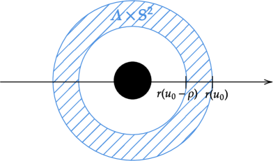
Figure 2. Cross section visualizing the set $\tilde{\Lambda}=\Lambda\times S^{2}$.

In order to compute this in more detail, we will prove that

$$\lim\limits_{\rho\rightarrow\infty}\lim\limits_{\alpha\rightarrow\infty}\frac{1}{f(\alpha)}\lim\limits_{u_{0}\rightarrow-\infty}\operatorname{tr}\Big{(}\eta\big{(}\chi_{\Lambda}(\Pi_{\varepsilon}^{-})_{kn}\chi_{\Lambda}\big{)}-\chi_{\Lambda}\eta\big{(}(\Pi_{\varepsilon}^{-})_{kn}\big{)}\chi_{\Lambda}\Big{)}$$ (4.2)

$$=\lim\limits_{\rho\rightarrow\infty}\lim\limits_{\alpha\rightarrow\infty}\frac{1}{f(\alpha)}\lim\limits_{u_{0}\rightarrow-\infty}\operatorname{tr}\Big{(}\eta\big{(}\chi_{\Lambda}\mathrm{Op}_{\alpha}(\mathfrak{A}_{0})\chi_{\Lambda}\big{)}-\chi_{\Lambda}\eta\big{(}\mathrm{Op}_{\alpha}(\mathfrak{A}_{0})\big{)}\chi_{\Lambda}\Big{)}\>,$$ (4.3)

where

$$\mathfrak{A}_{0}(\xi):=\begin{pmatrix}e^{M\xi}\chi_{(-\infty,0)}(\xi)&0\\ 0&e^{-M\xi}\chi_{(0,\infty)}(\xi)\end{pmatrix}\>.$$ (4.4)

(We will later see that the operators in (4.2) and (4.3) are well-defined and trace class). The notation $\mathfrak{A}_{0}$ is supposed to emphasize the connection to the $\varepsilon\rightarrow 0$ limit of $A_{\varepsilon}$. Since $\mathfrak{A}_{0}$ is diagonal the computation of (4.3) is much easier than the one for (4.2). In fact we have

$$\eqref{Limit Opa(b)}=\sum_{j=1}^{2}\lim\limits_{\rho\rightarrow\infty}\lim\limits_{\alpha\rightarrow\infty}\frac{1}{f(\alpha)}\lim\limits_{u_{0}\rightarrow-\infty}\operatorname{tr}\Big{(}\eta\big{(}\chi_{\Lambda}\mathrm{Op}_{\alpha}(\mathfrak{a}_{0,j})\chi_{\Lambda}\big{)}-\chi_{\Lambda}\eta\big{(}\mathrm{Op}_{\alpha}(\mathfrak{a}_{0,j})\big{)}\chi_{\Lambda}\Big{)}$$

with the scalar functions

$$\mathfrak{a}_{0,1}(\xi):=e^{M\xi}\chi_{(-\infty,0)}(\xi)\qquad\mathrm{and}\quad\mathfrak{a}_{0,2}(\xi):=e^{-M\xi}\chi_{(0,\infty)}(\xi)\>.$$ (4.5)

This reduces the computation of (4.3) to a problem for real-valued symbols for which many results are already established.

5. Properties of Pseudo-Differential Operators

In this section we will establish a few general results for pseudo-differential operators of the form $\mathrm{op}_{\alpha}(a)$ as in (3.10).

Lemma 5.1.

If the symbol $a$ is real-valued, measurable, bounded and only depends on $\xi$ and $\alpha$, i.e. $a(u,u^{\prime},\xi,\alpha)\equiv a(\xi,\alpha)$, then $\mathrm{op}_{\alpha}(a)$ is well-defined and self-adjoint. Moreover, for any Borel function $f$ defined on the spectrum of $\mathrm{op}_{\alpha}(a)$, we have

$$f(\mathrm{op}_{\alpha}(a))=\mathrm{op}_{\alpha}(f(a))\>.$$

Proof.

Note that

$$\mathrm{op}_{\alpha}(a)=\mathcal{F}\mathcal{M}_{a(./\alpha,\alpha)}\mathcal{F}^{-1}\>,$$ (5.1)

where $\mathcal{M}_{a(./\alpha,\alpha)}$ denotes the multiplication operator by $a(./\alpha,\alpha)$ and $\mathcal{F}$ the unitary extension of the Fourier transform on $L^{2}(\mathbb{R}^{d},C^{n})$ (since (5.1) holds for $C^{\infty}_{0}(\mathbb{R}^{d},\mathbb{C}^{n})$-functions and the right hand side defines a continuous operator on $L^{2}(\mathbb{R}^{d},C^{n})$). This also shows, that $\mathrm{op}_{\alpha}(a)$ is bounded (and therefore well-defined) and self-adjoint. Thus by the multiplicative form of the spectral theorem we have

$$f(\mathrm{op}_{\alpha}(a))=\mathcal{F}\mathcal{M}_{f(a(./\alpha,\alpha))}\mathcal{F}^{-1}=\mathrm{op}_{\alpha}(f(a))\>.$$

∎

The next lemma will be needed for consistency reasons when taking the limit $u_{0}\rightarrow-\infty$:

Lemma 5.2.

Let $U,V\subset\mathbb{R}^{d}$ be arbitrary Borel sets and $c\in\mathbb{R}^{d}$ an arbitrary vector. For any $u,u^{\prime},\xi\in\mathbb{R}^{d}$, $\alpha>0$ we transform a given symbol $a$ by

$$T_{c}(a)(u,u^{\prime},\xi,\alpha):=a(u+c,u^{\prime}+c,\xi,\alpha)\>.$$

Then there is a unitary transformation $t_{c}$ on $L^{2}(\mathbb{R}^{d},\mathbb{C}^{n})$ such that

$$t_{c}\>\chi_{U+c}\>\mathrm{op}_{\alpha}\big{(}T_{-c}(a)\big{)}\>\chi_{V+c}\>t_{c}^{-1}=\chi_{U}\>\mathrm{op}_{\alpha}(a)\>\chi_{V}\>.$$

In particular this leads to

$$\operatorname{tr}\Big{(}\chi_{U+c}\>\mathrm{op}_{\alpha}\big{(}T_{-c}(a)\big{)}\>\chi_{V+c}\Big{)}=\operatorname{tr}\big{(}\chi_{U}\>\mathrm{op}_{\alpha}(a)\>\chi_{V}\big{)}\>,$$

as well as for any $q>0$,

$$\big{\|}\chi_{U+c}\>\mathrm{op}_{\alpha}(T_{-c}(a))\>\chi_{V+c}\big{\|}_{q}=\big{\|}\chi_{U}\>\mathrm{op}_{\alpha}(a)\>\chi_{V}\big{\|}_{q}\>,$$

provided that the corresponding norms/traces are well-defined and finite.

Moreover, assuming in addition that $\mathrm{op}_{\alpha}(a)$ is self-adjoint, we conclude that for any Borel function $f$,

$$f\big{(}\chi_{U}\>\mathrm{op}_{\alpha}(a)\>\chi_{U}\big{)}=t_{c}\,f\big{(}\chi_{U+c}\>\mathrm{op}_{\alpha}(T_{-c}(a))\>\chi_{U+c}\big{)}\,t_{c}^{-1}\>,$$ (5.2)

with similar consequences for the trace and Schatten-norms.

Proof.

We will show that the desired unitary operator is given by the translation operator

$$t_{c}:L^{2}(\mathbb{R}^{d})\rightarrow L^{2}(\mathbb{R}^{d}),\quad f\mapsto f(.+c)\>,$$

(which is obviously unitary). Note that for any Borel set $W\subseteq\mathbb{R}^{d}$

$$\chi_{W+c}=t_{-c}\>\chi_{W}\>t_{c}\>,$$

and therefore

$$\chi_{U}\>\mathrm{op}_{\alpha}(a)\>\chi_{V} =t_{c}\>\chi_{U+c}\>t_{-c}\>\mathrm{op}_{\alpha}(a)\>t_{c}\>\chi_{V+c}t_{-c}\>.$$

By a change of coordinates we obtain for arbitrary $\psi\in C^{\infty}_{0}(\mathbb{R}^{d},\mathbb{C}^{n})$

$$\big{(}t_{-c}\>\mathrm{op}_{\alpha}(a)\>t_{c}\psi\big{)}(u)$$

$$=\big{(}\mathrm{op}_{\alpha}(a)\>t_{c}\psi\big{)}(u-c)=\frac{\alpha^{d}}{(2\pi)^{d}}\int d\xi\int du^{\prime}\>e^{-i\alpha\xi(u-c-u^{\prime})}\>a(u-c,u^{\prime},\xi,\alpha)\>\psi(u^{\prime}+c)$$

$$=\frac{\alpha^{d}}{(2\pi)^{d}}\int d\xi\int du^{\prime}\>e^{-i\alpha\xi(u-u^{\prime})}\>a(u-c,u^{\prime}-c,\xi,\alpha)\>\psi(u^{\prime})=\big{(}\mathrm{op}_{\alpha}\big{(}T_{-c}(a)\big{)}\psi\big{)}(x)\>.$$

Then the result follows by the unitary invariance of the trace and the Schatten-norms. For (5.2) we make use the multiplication operator version of the spectral theorem. This provides a unitary transformation $\phi$ and a suitable function $g$ such that

$$\chi_{U}\>\mathrm{op}_{\alpha}(a)\>\chi_{U}=\phi^{-1}\>\mathcal{M}_{g}\>\phi\>.$$

Combined with the previous discussion this implies

$$\chi_{U+c}\>\mathrm{op}_{\alpha}\big{(}T_{-c}(a)\big{)}\>\chi_{U+c}=(\phi\>t_{c})^{-1}\>\mathcal{M}_{g}\>(\phi\>t_{c})\>,$$

which is the multiplication operator representation of $\chi_{U+c}\>\mathrm{op}_{\alpha}\big{(}T_{-c}(a)\big{)}\>\chi_{U+c}$, because $\phi\>t_{c}$ is also a unitary operator. Therefore

$$f\big{(}\chi_{U+c}\>\mathrm{op}_{\alpha}(T_{-c}(a))\>\chi_{U+c}\big{)}=\big{(}\phi\>t_{c}\big{)}^{-1}\>\mathcal{M}_{f\circ g}\;\big{(}\phi\>t_{c}\big{)}=t_{c}^{-1}\>f\big{(}\chi_{U}\>\mathrm{op}_{\alpha}(a)\>\chi_{U}\big{)}\>t_{c}\>,$$

concluding the proof. ∎

Lemma 5.3.

Assume that the symbol $a$ of an operator $\mathrm{op}_{\alpha}(a)$ (restricted to a Borel set $U\subseteq\mathbb{R}^{n}$) satisfies

$$\int_{\mathbb{R}^{d}}d\xi\>\sqrt{\int_{U}du^{\prime}\>\big{\|}a(u,u^{\prime},\xi.\alpha)\big{\|}_{n\times n}^{2}}<\infty\>,\qquad\text{for any }u\in\mathbb{R}^{d}\text{ and }\alpha>0$$

(where $\|.\|_{n\times n}$ is the ordinary sup-norm on the $n\times n$-matrices). Then the integral-representation of $\mathrm{op}_{\alpha}(a)$ may be extended to all $L^{2}(\mathbb{R}^{d},\mathbb{C}^{n})$-functions and the $u^{\prime}$ and the $\xi$ integrations may be interchanged. Thus for any $\psi\in L^{2}(\mathbb{R}^{d},\mathbb{C}^{n})$, $\alpha>0$ and almost any $u\in\mathbb{R}^{d}$, the following equations hold,

$$\Big{(}\mathrm{op}_{\alpha}(a)\,\psi\Big{)}(u)= \Big{(}\frac{\alpha}{2\pi}\Big{)}^{d}\int_{\mathbb{R}^{d}}d\xi\int_{U}du^{\prime}\>e^{-i\alpha\xi\cdot(u-u^{\prime})}\>a(u,u^{\prime},\xi,\alpha)\>\psi(u^{\prime})$$

$$= \Big{(}\frac{\alpha}{2\pi}\Big{)}^{d}\int_{U}du^{\prime}\int_{\mathbb{R}^{d}}d\xi\>e^{-i\alpha\xi\cdot(u-u^{\prime})}\>a(u,u^{\prime},\xi,\alpha)\>\psi(u^{\prime})\>.$$

Proof.

We first show that, applying the Fubini-Tonelli theorem and Hölder’s inequality, the integrations may be interchanged, by estimating

$$\int_{\mathbb{R}^{d}}d\xi\int_{U}du^{\prime}\>\big{|}e^{-i\alpha\xi\cdot(u-u^{\prime})}a(u,u^{\prime},\xi,\alpha)\psi(u^{\prime})\big{|}$$

$$\leq\int_{\mathbb{R}^{d}}d\xi\;\sqrt{\int_{U}du^{\prime}\>\big{\|}a(u,u^{\prime},\xi,\alpha)\psi(u^{\prime})\big{\|}_{n\times n}^{2}}\;\big{\|}\psi\big{\|}_{L^{2}(\mathbb{R}^{d},\mathbb{C}^{n})}<\infty\>.$$

Next, we want to show that we can extend the integral representation to all $L^{2}(\mathbb{R}^{d},\mathbb{C}^{n})$-functions, i.e that the above integral indeed corresponds to $\big{(}\mathrm{op}_{\alpha}(a)\psi\big{)}(u)$. To this end let $(\psi_{n})_{n\in\mathbb{N}}$ be a sequence of $C^{\infty}_{0}(\mathbb{R}^{d},\mathbb{C}^{n})$-functions converging to $\psi$ with respect to the $L^{2}(\mathbb{R}^{d},\mathbb{C}^{n})$-norm. Then $\mathrm{op}_{\alpha}(a)\psi$ is by definition given by

$$\mathrm{op}_{\alpha}(a)\psi=\lim\limits_{n\rightarrow\infty}\mathrm{op}_{\alpha}(a)\psi_{n}\>,$$

where the convergence is with respect to the $L^{2}(\mathbb{R}^{d},\mathbb{C}^{n})$-norm. However, going over to a subsequence we can assume that this convergence also holds pointwise outside of the null set $N\subseteq\mathbb{R}^{d}$. Thus for any $u\in U\setminus N$ and $\alpha>0$ we can compute

$$\bigg{|}\Big{(}\frac{\alpha}{2\pi}\Big{)}^{d}\int_{\mathbb{R}^{d}}d\xi\int_{U}du^{\prime}\>e^{-i\alpha\xi\cdot(u-u^{\prime})}\>a(u,u^{\prime},\xi,\alpha)\>\psi(u^{\prime})-\big{(}\mathrm{op}_{\alpha}(a)\psi_{n}\big{)}(u)\bigg{|}$$

$$=\lim\limits_{n\rightarrow\infty}\bigg{|}\Big{(}\frac{\alpha}{2\pi}\Big{)}^{d}\int_{\mathbb{R}^{d}}d\xi\int_{U}du^{\prime}\>e^{-i\alpha\xi\cdot(u-u^{\prime})}\>a(u,u^{\prime},\xi,\alpha)\;\Delta\psi_{n}(u^{\prime})\bigg{|}$$

$$\leq\Big{(}\frac{\alpha}{2\pi}\Big{)}^{d}\int_{\mathbb{R}^{d}}d\xi\;\sqrt{\int_{\mathbb{R}^{d}}du^{\prime}\>\big{\|}a(u,u^{\prime},\xi,\alpha)\big{\|}_{n\times n}^{2}}\>\lim\limits_{n\rightarrow\infty}\|\Delta\psi_{n}\|^{2}_{L^{2}(\mathbb{R}^{d},\mathbb{C}^{n})}=0\>,$$

with $\Delta\psi_{n}:=\psi-\psi_{n}$. ∎

Remark 5.4.

We want to apply Lemma 5.3 to the operator $\chi_{\Lambda}(\Pi_{\varepsilon}^{-})_{kn}\chi_{\Lambda}$ with $\Lambda=(u_{0}-\rho,u_{0})$. By rescaling as before, we see that this operator is of the form $\mathrm{op}_{\alpha}(a)$ (restricted to $\Lambda$) with

$$a(u,u^{\prime},\xi,\alpha) =2\>\chi_{\Lambda}(u)\>\chi_{\Lambda}(u^{\prime})\>\chi_{(-\infty,0)}(\xi)\>e^{M\xi}$$

$$\quad\>\times\sum_{a,b=1}^{2}t_{ab}^{kn(\alpha\xi)}\begin{pmatrix}X_{a,+}^{kn(\alpha\xi)}(u)\overline{X_{b,+}^{kn(\alpha\xi)}(u^{\prime})}&X_{a,+}^{kn(\alpha\xi)}(u)\overline{X_{b,-}^{kn(\alpha\xi)}(u^{\prime})}\\ X_{a,-}^{kn(\alpha\xi)}(u)\overline{X_{b,+}^{kn(\alpha\xi)}(u^{\prime})}&X_{a,-}^{kn(\alpha\xi)}(u)\overline{X_{b,-}^{kn(\alpha\xi)}(u^{\prime})}\end{pmatrix}\>.$$

Note that, a-priori, the integral representation of this operator is well-defined only for $C^{\infty}_{0}(\mathbb{R})^{2}$-functions with support in $\Lambda$. In order to extend the integral representation to all $L^{2}(\Lambda,\mathbb{C}^{2})$-functions it suffices to verify the condition in Lemma 5.3. To this end we note that, due to Lemma 2.3, for given $u_{2}>u_{0}$, we have

$$|X_{a,i}^{kn(\alpha\xi)}(u)|<1+ce^{du}\>,$$

for any $a\in\{1,2\}$, $i\in\{+,-\}$, $u<u_{2}$ and $\xi\in\mathbb{R}$, where the constants $c,d>0$ are independent of $\xi$. Also using that the transmission coefficients $t_{ab}$ are always bounded by $1/2$, we obtain the estimate

$$\|a(u,u`,\xi,\alpha)\|_{n\times n}\leq C\>e^{M\xi}\>\chi_{(-\infty,0)}(\xi)\>\chi_{\Lambda}(u)\>\chi_{\Lambda}(u^{\prime})$$

for any $\alpha>0$ with $C$ independent of $u$, $u^{\prime}$ and $\xi$. Thus for any $u\in\Lambda$ and $\alpha>0$ we have

$$\int d\xi\;\sqrt{\int du^{\prime}\>\|a(u,u^{\prime},\xi.\alpha)\|_{n\times n}^{2}}=C\int_{-\infty}^{0}d\xi\;\sqrt{\int_{u_{0}-\rho}^{u_{0}}du^{\prime}\>e^{2M\xi}}=C\frac{\sqrt{\rho}}{M}<\infty\>.$$

Clearly, the entire expression vanishes for $u\notin\Lambda$.
This shows that we can indeed apply Lemma 5.3 to $\chi_{\Lambda}(\Pi_{\varepsilon}^{-})_{kn}\chi_{\Lambda}$, meaning that the corresponding integral representation can be applied to any $L^{2}(\Lambda,\mathbb{C}^{2})$ function, and the $u^{\prime}$- and $\xi$-integrations may be interchanged. Moreover, due to the characteristic functions in the symbol, we can even extend the integral representation to all functions in $L^{2}(\mathbb{R},\mathbb{C}^{2})$.   $\Diamond$

Lemma 5.5.

Let $a(u,u^{\prime},\xi,\alpha)=a(u,\xi,\alpha)$ and $b(u,u^{\prime},\xi,\alpha)=b(u^{\prime},\xi,\alpha)$ be symbols such that $\mathrm{Op}_{\alpha}(a)$ and $\mathrm{Op}_{\alpha}(b)$ are well-defined and the following two conditions hold:

• The operator $A$ defined for any $\psi\in L^{2}(\mathbb{R}^{d},\mathbb{C}^{n})$ by

  $$(A\psi)(u):=\int_{\mathbb{R}^{n}}e^{-i\xi u}\>a(u,\xi/\alpha,\alpha)\>\psi(\xi)\>d\xi\>,$$

  is bounded on  $L^{2}(\mathbb{R}^{d},\mathbb{C}^{n})$.

• The operator $B$ defined for any Schwartz function $\psi\in L^{2}(\mathbb{R}^{d},\mathbb{C}^{n})$ by

  $$(B\psi)(\xi):=\frac{1}{(2\pi)^{d}}\int_{\mathbb{R}^{n}}e^{i\xi u^{\prime}}\>b(u^{\prime},\xi/\alpha,\alpha)\>\psi(u^{\prime})\>du^{\prime}\>,$$

  may be continuously extended to $L^{2}(\mathbb{R}^{d},\mathbb{C}^{n})$.

Then

$$\mathrm{Op}_{\alpha}(a)\>\mathrm{Op}_{\alpha}(b)=\mathrm{Op}_{\alpha}(ab)\>.$$

Proof.

We first note that, due to condition (i),

$$\mathrm{Op}_{\alpha}(a)=A\>\mathcal{F}^{-1}\>,$$

as both sides define continuous operators on $L^{2}(\mathbb{R}^{d},\mathbb{C}^{n})$ and agree on the Schwartz functions (where again $\mathcal{F}$ is the continuous extension of the Fourier transform to $L^{2}(\mathbb{R}^{d},\mathbb{C}^{n})$). Similarly, we conclude that

$$\mathrm{Op}_{\alpha}(b)=\mathcal{F}\>B\>.$$

This yields

$$\mathrm{Op}_{\alpha}(a)\>\mathrm{Op}_{\alpha}(b)=A\>B\>,$$

and for any Schwartz function $\psi$ we have

$$\mathrm{Op}_{\alpha}(a)\mathrm{Op}_{\alpha}(b)\psi=AB\psi=\int_{\mathbb{R}^{d}}d\xi\int_{\mathbb{R}^{n}}du^{\prime}\>e^{-i\alpha\xi(u-u^{\prime})}a(u,\xi,\alpha)b(u^{\prime},\xi,\alpha)\psi(u^{\prime})\>.$$

Note that as $\mathrm{Op}_{\alpha}(a)$ and $\mathrm{Op}_{\alpha}(b)$ are bounded operators, so is $\mathrm{Op}_{\alpha}(a)\>\mathrm{Op}_{\alpha}(b)$. This concludes the proof by continuous extension and by the definition of $\mathrm{Op}_{\alpha}(ab)$. ∎

Remark 5.6.

• In what follows we often apply the previous Lemma in the case that

  $$b(u^{\prime},\xi,\alpha)=\chi_{U}(\xi)$$

  for some measurable set $U\subseteq\mathbb{R}^{d}$. Then condition (ii) of Lemma 5.5 is obviously fulfilled, because for any Schwartz function $\psi$ we have

  $$\|B\psi\|=\|\chi_{\alpha U}\>\mathcal{F}^{-1}\psi\|\leq\|\mathcal{F}^{-1}\psi\|=\|\psi\|\>.$$

• Moreover, in the following, the symbol $a$ is sometimes independent of $u$ and bounded by a constant $C>0$, then for any $\psi\in L^{2}(\mathbb{R}^{d},\mathbb{C}^{n})$ it follows that

  $$\|A\psi\|=\|a(./\alpha,\alpha)\>\mathcal{F}\psi\|\leq C\|\psi\|\>.$$

  Therefore, condition (i) in Lemma 5.5 is also fulfilled.

• Another case we will consider later is that $a$ is scalar-valued and continuous with compact support

  $$\operatorname{supp}a\subseteq B_{l}(v)\times B_{r}(\mu)\>.$$

  Then from the following argument we conclude that $A$ also fulfills condition (i) from Lemma 5.5. Take $\psi\in L^{2}(\mathbb{R}^{d})$ arbitrary and consider

  $$\int|A\psi(u)|^{2}\>du$$

  $$=\int_{B_{l}(v)}du\int_{B_{r}(\mu)}d\xi\int_{B_{r}(\mu)}d\xi^{\prime}\>e^{-iu(\xi^{\prime}-\xi)}\>\overline{\psi(\xi)}\>\psi(\xi^{\prime})\>\overline{a(u,\xi/\alpha,\alpha)}\>a(u,\xi^{\prime}/\alpha,\alpha)$$

  Here we may interchange the order of integration due to the Fubini-Tonelli Theorem since

  $$\int_{B_{l}(v)}du\int_{B_{r}(\mu)}d\xi\int_{B_{r}(\mu)}d\xi^{\prime}\>\Big{|}\overline{\psi(\xi)}\>\psi(\xi^{\prime})\>\overline{a(u,\xi/\alpha,\alpha)}\>a(u,\xi^{\prime}/\alpha,\alpha)\Big{|}$$

  $$\leq C^{2}\>\text{vol}(B_{l}(v))\>\|\psi\|_{L^{1}(B_{r}(\mu),\mathbb{C}^{2})}^{2}<\infty\>,$$

  where $C$ is a bound for the absolute value of the continuous and compactly supported function $a$. Note that $L^{2}(B_{r}(\mu),\mathbb{C}^{2})\subseteq L^{1}(B_{r}(\mu),\mathbb{C}^{2})$ since $B_{r}(\mu)$ is bounded. We then obtain

  $$\int|A\psi(u)|^{2}\>du$$

  $$=\int d\xi\>\overline{\psi(\xi)}\int d\xi^{\prime}\>\psi(\xi^{\prime})\underbrace{\int du\>e^{-iu(\xi^{\prime}-\xi)}\>\overline{a(u,\xi/\alpha,\alpha)}\>a(u,\xi^{\prime}/\alpha,\alpha)}_{=:\tilde{a}(\xi,\xi^{\prime})}$$

  $$\leq\|\psi\|\int|\psi(\xi)|\>\|\tilde{a}(\xi,.)\|\>d\xi\leq\|\psi\|^{2}\sqrt{\int d\xi\int d\xi^{\prime}\>|\tilde{a}(\xi,\xi^{\prime})|^{2}}\>,$$

  where the function $\tilde{a}$ is again continuous and compactly supported, which makes the last integral finite. We remark that in the last line we again applied Hölder’s inequality.

  This estimate shows that condition (i) from Lemma 5.5 is again satisfied.   $\Diamond$

6. Trace of the Limiting Operator

In this section we will only consider the operator $\mathrm{Op}_{\alpha}(\mathfrak{a}_{0,1})$ in (4.5). Of course, the same methods apply to $\mathrm{Op}_{\alpha}(\mathfrak{a}_{0,2})$.

Notation 6.1.

In the following it might happen that in the symbol $a$ we can factor out a characteristic function in $\xi$, i.e.

$$a(\xi,u,u^{\prime},\alpha)=\chi_{\Omega}(\xi)\>\tilde{a}(\xi,u,u^{\prime},\alpha)\>.$$

In this case, we will sometimes denote the characteristic function in $\xi$ corresponding to the set $\Omega$ by $I_{\Omega}$. This is to avoid confusion with the characteristic function $\chi_{\Lambda}$ in the variables $u$ or $u^{\prime}$.

Remark 6.2.

Note that, in view of Lemma 5.3, the operator $\mathrm{Op}_{\alpha}(\mathfrak{a}_{0,1})$ is well-defined when restricted to any bounded subset of $\mathbb{R}$. In particular, $\chi_{\Lambda}\mathrm{Op}_{\alpha}(\mathfrak{a}_{0,1})\chi_{\Lambda}$ is well-defined on all of $L^{2}(\mathbb{R})$ and the integral representation also holds on $L^{2}(\mathbb{R})$.

6.1. Idea for Smooth Functions

The general idea is to make use of the following one-dimensional result by Widom [30].

Theorem 6.3.

Let $K,J\subseteq\mathbb{R}$ intervals, $f\in C^{\infty}(\mathbb{R})$ be a smooth function with $f(0)=0$ and $a\in C^{\infty}(\mathbb{R}^{2})$ a complex-valued Schwartz function which we identify with the symbol $a(u,u^{\prime},\xi,\alpha)\equiv a(u,\xi)$ for any $u,u^{\prime},\xi,\alpha\in\mathbb{R}$. Moreover, for any symbol $b$ we denote its symmetric localization by

$$A(b):=\frac{1}{2}\Big{(}\chi_{K}\,\mathrm{Op}_{\alpha}\big{(}I_{J}\,b\big{)}\,\chi_{K}+\big{(}\chi_{K}\mathrm{Op}_{\alpha}\big{(}I_{J}\,b\big{)}\chi_{K}\big{)}^{*}\Big{)}\>,$$ (6.1)

(recall that $I_{J}$ is the characteristic function corresponding to $J\subseteq\mathbb{R}$ with respect to the variable $\xi$). Then

$$\operatorname{tr}\Big{(}f(A(a))-\chi_{K}\>\mathrm{Op}_{\alpha}\big{(}I_{J}\,f(a)\big{)}\>\chi_{K}\Big{)}=\frac{1}{4\pi^{2}}\log(\alpha)\sum_{i}U\big{(}a(v_{i});f\big{)}+\mathcal{O}(1)\>,$$

where $v_{i}$ are the vertices of $K\times J$ (see Figure 3)

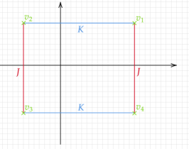
(a) Vertices if $K$ and $J$ are both finite: There are in total four vertices.

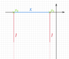
(b) Vertices if $K$ is finite and $J$ is infinite: There are only two vertices.

Figure 3. Illustration with examples of the “vertices” in Theorem 6.3.

and

$$U(\tilde{a};f):=\int_{0}^{1}\frac{1}{t(1-t)}\>\Big{(}f(t\tilde{a})-tf(\tilde{a})\Big{)}\>dt\qquad\text{for any }\tilde{a}\in\mathbb{R}\>.$$

Remark 6.4.

• To be precise, Widom considered operators with kernels

  $$\frac{\alpha}{2\pi}\int dy\int d\xi\>e^{\mathbf{+}i\alpha\xi(u-u^{\prime})}\>a(u,\xi)$$

  but the results can clearly be transferred using the transformation $\xi\rightarrow-\xi$.

• Moreover, Widom considers operators of the form $\mathrm{Op}_{\alpha}(a)$ whose integral representation extends to all of $L^{2}(K)$. We note that, in view of Lemma 5.3, this assumption holds for any operator $\mathrm{Op}_{\alpha}(a)$ with Schwartz symbol $a=a(u,\xi)$, even if, a-priori, the integral representation holds only when inserting Schwartz functions.   $\Diamond$

We want to apply the above theorem with $J=(-\infty,0)$ and $K=(u_{0}-\rho,u_{0})$, where we choose $f$ as a suitable approximation of the function $\eta$ (again with $f(0)=0$) and $a$ an approximation of the diagonal matrix entries $\mathfrak{a}_{0,1/2}$ in (4.4) and (4.5). For ease of notation, we only consider $a\approx\mathfrak{a}_{0,1}$, noting that our methods apply similarly to $\mathfrak{a}_{0,2}$. To be more precise, we first introduce the smooth non-negative cutoff functions $\Psi,\Phi\in C^{\infty}(\mathbb{R})$ with

$$\Psi(\xi)=\begin{cases}1\>,\quad\xi\leq 0\\ 0\>,\quad\xi>1\end{cases}\qquad\text{and}\qquad\Phi(u)=\begin{cases}1\>,\quad u\in[-\rho,0]\\ 0\>,\quad u\notin(-\rho-1,1)\>,\end{cases}$$ (6.2)

and set $\Phi_{u_{0}}(x):=\Phi(x-u_{0})$. Then we may introduce $a$ as the function

$$a(u,\xi):=\Psi(\xi)\>\Phi_{u_{0}}(u)\>e^{M\xi}\>.$$ (6.3)

For a plot of $a$ see Figure 4.

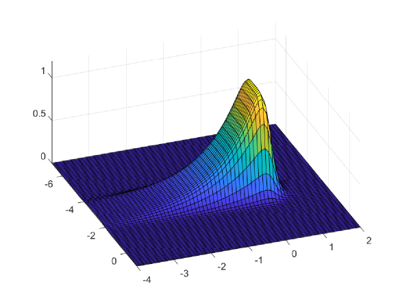
Figure 4. Plot of the function $a$ from (6.3).

Note that then $a$ is a Schwartz function and

$$\chi_{K}\>\mathrm{Op}_{\alpha}(I_{J}\,a)\>\chi_{K}=\chi_{K}\>\mathrm{Op}_{\alpha}(\mathfrak{a}_{0,1})\>\chi_{K}\>.$$

Moreover, the resulting symbol clearly fulfills the condition of Lemma 5.3, so we can extend the corresponding integral representation to all $L^{2}(\mathbb{R},\mathbb{C})$-functions. In addition, the operator is self-adjoint, because of Lemma 5.1. This implies that we can leave out the symmetrization in (6.1), i.e.

$$A(a)=\chi_{K}\>\mathrm{Op}_{\alpha}(I_{J}\>a)\>\chi_{K}=\chi_{K}\>\mathrm{Op}_{\alpha}(\mathfrak{a}_{0,1})\>\chi_{K}\>.$$

Furthermore, due to Lemma 5.1, we may pull out any function $f$ as in the above Theorem  6.3 in the sense that

$$\chi_{K}\>\mathrm{Op}_{\alpha}\big{(}I_{J}\>f(a)\big{)}\>\chi_{K}=\chi_{K}\>\mathrm{Op}_{\alpha}\big{(}f(\mathfrak{a}_{0,1})\big{)}\>\chi_{K}=\chi_{K}\>f(\mathrm{Op}_{\alpha}(\mathfrak{a}_{0,1}))\>\chi_{K}\>,$$

where we used that $\mathfrak{a}_{0,1}$ vanishes outside $J$ and that $f(0)=0$.

In our application the vertices of $K\times J$ are (similar as in Figure 3 (B)) given by

$$v_{1}=(u_{0},0)\qquad\text{and}\qquad v_{2}=(u_{0}-\rho,0)\>,$$

and thus

$$a(v_{i})=1\>,\qquad\text{for any }i=1,2\>,$$

leading to

$$\operatorname{tr}\Big{(}f\big{(}\chi_{K}\mathrm{Op}_{\alpha}(\mathfrak{a}_{0,1})\chi_{K}\big{)}-\chi_{K}f\big{(}\mathrm{Op}_{\alpha}(\mathfrak{a}_{0,1})\big{)}\chi_{K}\Big{)}=\frac{1}{2\pi^{2}}\>\log(\alpha)\>U(1;f)+\mathcal{O}(1)\>,$$ (6.4)

valid for any $f\in C^{\infty}(\mathbb{R})$ with $f(0)=0$.

Note that, using Lemma 5.2 and the fact that $\mathfrak{a}_{0,1}$ does not depend on $u$ or $u^{\prime}$, the $\mathcal{O}(1)$-term does not change when varying $u_{0}$, and therefore the result stays same when we take the limit $u_{0}\rightarrow-\infty$. We need to keep this in mind because we shall take the limit $u_{0}\rightarrow-\infty$ before the limit $\alpha\rightarrow\infty$ (cf. (4.1)).

6.2. A Few More Technical Results

In order to estimate the errors in Theorem 6.3 caused by using a smooth approximation of $\eta$, we need a few more technical results. The first lemma shows that $\mathrm{Op}_{\alpha}(b)$ is bounded with respect to the operator norm uniformly in $\alpha$ as long as $b\in S^{(n,m,k)}(\mathbb{R}^{d})$.

Lemma 6.5.

[24, Lemma 3.9] Let $b\in S^{(k,k,d+1)}(\mathbb{R}^{d})$ a symbol, $k:=\lfloor d/2\rfloor+1$ a parameter, $l_{0}>0$ a constant and $l,r>0$ such that $\alpha lr\geq l_{0}$. Then

$$\|\mathrm{Op}_{\alpha}(b)\|_{\infty}\leq C_{l_{0}}\>N^{(k,k,d+1)}(b;r,l)\>,$$

with $C>0$ only depending on $d$ and $l_{0}$.

Example 6.6.

Lemma 6.5 can be used to estimate the operator norm of $\mathrm{Op}_{\alpha}(\mathfrak{a}_{0,1})$. To this end, we first use Lemma 5.5 together with Remark 5.6 to obtain

$$\mathrm{Op}_{\alpha}(\mathfrak{a}_{0,1})=\mathrm{Op}_{\alpha}(\tilde{a})\>\mathrm{Op}_{\alpha}(\chi_{(0,\infty)})\>,$$

with the symbol $\tilde{a}(u,u^{\prime},\xi)=\tilde{a}(\xi)=\Psi(\xi)e^{M\xi}$ and with the cutoff function $\Psi$ as in (6.2). Since the symbol $\tilde{a}$ is contained in $S^{(1,1,2)}$ we can estimate the operator norm of $\mathrm{Op}_{\alpha}(\tilde{a})$ using Lemma 6.5

$$\|\mathrm{Op}_{\alpha}(\tilde{a})\|_{\infty}\leq C_{l_{0}}\>N^{(1,1,2)}(\tilde{a};1,1)\>.$$

Finally, making use of the fact that $\mathrm{Op}_{\alpha}(\chi_{(-\infty,0)})$ is a projection operator (which follows from Lemma 5.1), we conclude that

$$\|\mathrm{Op}_{\alpha}(\mathfrak{a}_{0,1})\|_{\infty} =\|\mathrm{Op}_{\alpha}(\tilde{a})\>\mathrm{Op}_{\alpha}(\chi_{(0,\infty)})\|_{\infty}\leq\|\mathrm{Op}_{\alpha}(\tilde{a})\|_{\infty}\>\|\mathrm{Op}_{\alpha}(\chi_{(0,\infty)})\|_{\infty}$$

$$\leq C_{l_{0}}\>N^{(1,1,2)}(\tilde{a};1,1)\leq\tilde{C}_{M,l_{0}}$$

for any $\alpha\geq l_{0}$, where the constant $\tilde{C}_{M,l_{0}}$ only depends on $M$, $\Psi$ and $l_{0}$.  $\Diamond$

The next technical lemma will be used to estimate the error term caused by replacing $f$ in Theorem 6.3 by a non-smooth function.

Lemma 6.7.

[26, Cor. 2.11, Cond. 2.9, Thm. 2.10]
Let $q,r>0$ parameters, $n\geq 2$ a natural number and $f\in C^{n}_{0}(-r,r)$. Let $\mathfrak{S}\subset\text{\rm{L}}(\mathfrak{H})$ (with a Hilbert space $\mathfrak{H}$) be a $q$-normed ideal such that there is $\sigma\in(0,1]$ with

$$(n-\sigma)^{-1}<q\leq 1\>.$$

Moreover, consider a self-adjoint operator $A$ on $D(A)\subseteq\mathfrak{H}$ and a projection operator $P$ such that $PD(A)\subseteq D(A)$ and $|PA(\mathds{1}-P)|^{\sigma}\in\mathfrak{S}$ and $PA(\mathds{1}-P)$ extends to a bounded operator. Then

$$\|f(PAP)P-Pf(A)\|_{\mathfrak{S}}\leq C\max_{0\leq k\leq n}\Big{(}r^{k}\|f^{(k)}\|_{L^{\infty}}\Big{)}\>r^{-\sigma}\>\big{\|}|PA(\mathds{1}-P)|^{\sigma}\big{\|}_{\mathfrak{S}}$$

with a constant $C$ independent of $A$, $P$ and $f$.

In order to also estimate the error caused by a non-differentiable function $f$ in Theorem 6.3, we need the next lemma.

Lemma 6.8.

[26, Thm. 2.10 and Cond. 2.3]
Let $n\geq 2$ a natural number, $f\in C^{n}(\mathbb{R}\setminus\{x_{0}\})\cap C(\mathbb{R})$ with $x_{0}\in\mathbb{R}$, such that there exist $\gamma,R>0$ with

$${\,\vrule depth=3.0pt,height=9.0pt}{\vrule depth=3.0pt,height=9.0pt}{\vrule depth=3.0pt,height=9.0pt}{\vrule depth=3.0pt,height=9.0pt}\,f{\,\vrule depth=3.0pt,height=9.0pt}{\vrule depth=3.0pt,height=9.0pt}{\vrule depth=3.0pt,height=9.0pt}{\vrule depth=3.0pt,height=9.0pt}\,_{n}:=\max_{0\leq k\leq n}\sup_{x\neq x_{0}}|f^{(k)}(x)|\cdot|x-x_{0}|^{-\gamma+k}<\infty\>,$$

and $\operatorname{supp}f\subseteq[x_{0}-R,x_{0}+R]$. Let $\mathfrak{S}$, $A$ and $P$ as in Lemma 6.7 with $\sigma<\gamma$, then

$$\big{\|}f(PAP)P-Pf(A)\big{\|}_{\mathfrak{S}}\leq C\>{\,\vrule depth=3.0pt,height=9.0pt}{\vrule depth=3.0pt,height=9.0pt}{\vrule depth=3.0pt,height=9.0pt}{\vrule depth=3.0pt,height=9.0pt}\,f{\,\vrule depth=3.0pt,height=9.0pt}{\vrule depth=3.0pt,height=9.0pt}{\vrule depth=3.0pt,height=9.0pt}{\vrule depth=3.0pt,height=9.0pt}\,_{n}\>R^{\gamma-\sigma}\>\big{\|}|PA(\mathds{1}-P)|^{\sigma}\big{\|}_{\mathfrak{S}}\>.$$

Example 6.9.

Ultimately we want to apply Lemma 6.8 to $\eta$ (times a cutoff function). Therefore we introduce the function

$$f(x):=\eta(x)\,\Psi_{1}(x)\>,\qquad\text{for any }x\in\mathbb{R}\>,$$

with a smooth non-negative function $\Psi_{1}$ such that

$$\operatorname{supp}\Psi_{1}=\Big{[}-\frac{3}{4},\>\frac{3}{4}\Big{]}\qquad\text{and}\qquad\Psi_{1}\big{|}_{\left[-\frac{1}{2},\>\frac{1}{2}\right]}\equiv 1\>.$$

Note that $f$ then satisfies the conditions of Lemma 6.8 for any $n\in\mathbb{N}$, $\gamma<1$ arbitrary, $R=3/4$ and $x_{0}=0$ .

This gives an idea how Lemma 6.8 can be used to estimate the error in Theorem 6.3 caused by functions like $\eta$, which are not differentiable everywhere.   $\Diamond$

Note that later we want to apply the previous lemmas to $A=\mathrm{Op}_{\alpha}(\mathfrak{a}_{0,1})$ and $P=\chi_{\Lambda}$. Moreover, in what follows we will often use the notation

$$P_{\Omega,\alpha}:=\mathrm{Op}_{\alpha}(\chi_{\Omega})$$

for some measurable $\Omega\subseteq\mathbb{R}^{d}$, which emphasizes that this is a projection operator (this and that it is well-defined follows from Lemma 5.1).

In order to complete the error estimates, one finally needs to control the therm $\||PA(\mathds{1}-P)|^{\sigma}\|_{\mathfrak{S}}$. This can be done with the following lemma, which is a modification of Lemma 4.6 from [25].

Lemma 6.10.

Let $u_{0}\in\mathbb{R}$, $\rho\geq 1$ arbitrary numbers, $\Lambda=(u_{0}-\rho,u_{0})$, $\Omega=(-\infty,0)$ intervals and take numbers $q\in(0,1]$, $n=\lfloor q^{-1}\rfloor+1$, $m=\lfloor 2q^{-1}\rfloor+1$, $0<l\leq\rho$ and $\alpha\geq 2$ with $\alpha lr\geq l_{0}\geq 1$. Moreover, let $b\in S^{(n,m)}(\mathbb{R})$ be a symbol with support contained in $B_{l}(v)\times B_{r}(\mu)$ for some $v,\mu\in\mathbb{R}$, then

$$\big{\|}\chi_{\Lambda}\mathrm{Op}_{\alpha}(I_{\Omega}\>b)(1-\chi_{\Lambda})\big{\|}_{q}^{q} \leq C_{q,l_{0}}(\rho,r)^{q}\>\ln(\alpha)\>N^{(1,2)}(b;1,1)^{q}+\tilde{C}_{q,l_{0}}\>N^{(n,m)}(b;l,r)^{q}\>,$$

where all the constants are independent of $u_{0}$.

In order to prove this Lemma we need to make use of Theorem 3.2, Theorem 4.2 and Corollary 4.7 from [25]. Therefore, we first state them (applied to the cases needed):

Theorem 6.11.

[25, Theorem 3.2, (3.5)] (case $t=0$, $d=1$) Let $q\in(0,1]$ and $h_{1}$ and $h_{2}$ be two $L^{\infty}(\mathbb{R})$-functions whose supports have distance at least $R$. Moreover, we choose a symbol $b\in S^{n,m}(\mathbb{R})$ for $m\geq n$ with $\operatorname{supp}b\subseteq B_{l}(v)\times B_{r}(\mu)$ for some $v,\mu\in\mathbb{R}$. Then, for any choice of parameters $q\in[0,1)$, $\alpha lr\geq l_{0}>0$ and $R\geq l$, the following inequality holds,

$$\|h_{1}\mathrm{Op}_{\alpha}(b)h_{2}\|_{q}\leq C_{q,m,l_{0}}\>\|h_{1}\|_{L^{\infty}}\>\|h_{2}\|_{L^{\infty}}\>(\alpha Rr)^{1/q-m}\>N^{(n,m)}(b;l,r)\>.$$

Theorem 6.12.

[25, Theorem 4.2, (2.11), (3.5), Section 4.1](case $d=1$) Let $q=(0,1]$, $\alpha lr\geq l_{0}>0$, $n=\lfloor q^{-1}\rfloor+1$ and $m=\lfloor 2q^{-1}\rfloor+1$. Let again $b\in S^{(n,m)}(\mathbb{R})$ be a symbol with support contained in $B_{l}(v)\times B_{r}(\mu)$ for some $v,\mu\in R$. Then

$$\|\chi_{(-\infty,0)}\>\mathrm{Op}_{\alpha}(b)\>\chi_{(0,\infty)}\|_{q},\|\chi_{(0,\infty)}\mathrm{Op}_{\alpha}(b)\chi_{(-\infty,0)}\|_{q}\leq C_{q,l_{0}}\>N^{(n,m)}(b;l,r)\>$$

$$\|P_{\alpha,(-\infty,0)}\>\mathrm{Op}_{\alpha}(b)\>P_{\alpha,(0,\infty)}\|_{q},\|P_{\alpha,(0,\infty)}\mathrm{Op}_{\alpha}(b)P_{\alpha,(-\infty,0)}\|_{q}\leq C_{q,l_{0}}\>N^{(n,m)}(b;l,r)\>.$$

Corollary 6.13.

[25, Corollary 4.7](case $d=1$) For any two open bounded intervals $K,J$ as well as numbers $q\in(0,1]$ and $\alpha\geq 2$, the following inequality holds,

$$\|\chi_{K}P_{J,\alpha}(1-\chi_{K})\|_{q}\leq C_{q}(K,J)(\ln\alpha)^{1/q}\>.$$

In preparation of the proof of Lemma 6.10 we will first prove the following modified version of Theorem 6.12.

Lemma 6.14.

Let $\Lambda=(u_{0}-\rho,u_{0})$ as before, $q=(0,1]$, $\alpha lr\geq l_{0}\geq 1$ with $0<l\leq\rho$, $n=\lfloor q^{-1}\rfloor+1$ and $m=\lfloor 2q^{-1}\rfloor+1$. Let again $b\in S^{(n,m)}(\mathbb{R})$ be a symbol with support contained in $B_{l}(v)\times B_{r}(\mu)$ for some $v,\mu\in R$. Then

$$\big{\|}\chi_{\Lambda}\>\mathrm{Op}_{\alpha}(b)\>(1-\chi_{\Lambda})\big{\|}_{q}\leq C_{q,m,l_{0}}\>N^{(n,m)}(b;l,r)$$

with $C_{q,m,l_{0}}$ independent of $u_{0}$ and $\rho$.

Proof.

We first note that, due to Lemma 5.2,

$$\big{\|}\chi_{\Lambda}\>\mathrm{Op}_{\alpha}(b)\>(1-\chi_{\Lambda})\big{\|}_{q}=\big{\|}\chi_{(-\rho,0)}\mathrm{Op}_{\alpha}(T_{u_{0}}(b))(1-\chi_{(-\rho,0)})\big{\|}_{q}\>.$$

We take the $q^{\text{th}}$ power and apply the $q$-triangle inequality to obtain

$$\|\chi_{(-\rho,0)}\mathrm{Op}_{\alpha}(T_{u_{0}}(b))(1-\chi_{(-\rho,0)})\|_{q}^{q}=\|\chi_{(-\rho,0)}\mathrm{Op}_{\alpha}(T_{u_{0}}(b))(\chi_{(-\infty,-\rho)}+\chi_{(0,\infty)})\|_{q}^{q}$$

$$\leq C\|\chi_{(-\rho,0)}\mathrm{Op}_{\alpha}(T_{u_{0}}(b))\chi_{(-\infty,-\rho)}\|_{q}^{q}+C\|\chi_{(-\rho,0)}\mathrm{Op}_{\alpha}(T_{u_{0}}(b))\chi_{(0,\infty)}\|_{q}^{q}$$

$$=C\|(\chi_{(-\rho,\infty)}-\chi_{(0,\infty)})\mathrm{Op}_{\alpha}(T_{u_{0}}(b))\chi_{(-\infty,-\rho)}\|_{q}^{q}$$

$$\quad\>+C\|(\chi_{(-\infty,0)}-\chi_{(-\infty,-\rho)})\mathrm{Op}_{\alpha}(T_{u_{0}}(b))\chi_{(0,\infty)}\|_{q}^{q}$$

$$\begin{split}&\leq C\|\chi_{(-\rho,\infty)}\mathrm{Op}_{\alpha}(T_{u_{0}}(b))\chi_{(-\infty,-\rho)}\|_{q}^{q}+C\|\chi_{(0,\infty)}\mathrm{Op}_{\alpha}(T_{u_{0}}(b))\chi_{(-\infty,-\rho)}\|_{q}^{q}\\ &\quad\>+C\|\chi_{(-\infty,0)}\mathrm{Op}_{\alpha}(T_{u_{0}}(b))\chi_{(0,\infty)}\|_{q}^{q}+C\|\chi_{(-\infty,-\rho)}\mathrm{Op}_{\alpha}(T_{u_{0}}(b))\chi_{(0,\infty)}\|_{q}^{q}\end{split}$$ (6.5)

with a constant $C>0$ depending only on $q$. Using again Lemma 5.2, we obtain

$$\|\chi_{(-\rho,\infty)}\mathrm{Op}_{\alpha}(T_{u_{0}}(b))\chi_{(-\infty,-\rho)}\|_{q}^{q}=\|\chi_{(0,\infty)}\mathrm{Op}_{\alpha}(T_{u_{0}-\rho}(b))\chi_{(-\infty,0)}\|_{q}^{q}\>.$$

Using this relation, we can apply Lemma 6.12 to the first and the third term in (LABEL:EstProof4.2Mod),

$$\|\chi_{(-\rho,\infty)}\mathrm{Op}_{\alpha}(T_{u_{0}}(b))\chi_{(-\infty,-\rho)}\|_{q} \leq C_{q,l_{0}}N^{(n,m)}(T_{u_{0}-\rho}(b);l,r)\>,$$

$$\|\chi_{(-\infty,0)}\mathrm{Op}_{\alpha}(T_{u_{0}}(b))\chi_{(0,\infty)}\|_{q} \leq C_{q,l_{0}}N^{(n,m)}(T_{u_{0}}(b);l,r)\>.$$

Note that, by definition of $N^{(n,m)}$, we know that, for any $u\in\mathbb{R}$,

$$N^{(n,m)}(T_{u}(b);l,r)=N^{(n,m)}(b;l,r)\>,$$

which yields that

$$\|\chi_{(-\rho,\infty)}\mathrm{Op}_{\alpha}(T_{u_{0}}(b))\chi_{(-\infty,-\rho)}\|_{q}\>,\>\|\chi_{(-\infty,0)}\mathrm{Op}_{\alpha}(T_{u_{0}}(b))\chi_{(0,\infty)}\|_{q}\leq C_{q,l_{0}}N^{(n,m)}(b;l,r)\>.$$

For the second and fourth term, we apply Theorem 6.11, noting that the numbers $n,m$ in the claim clearly satisfy the corresponding conditions in this theorem. Using the inequalities

$$\frac{1}{q}-m\leq 0$$

and $\alpha r\rho\geq 1$, we obtain the estimate

$$\|\chi_{(-\infty,-\rho)}\mathrm{Op}_{\alpha}(T_{u_{0}}(b))\chi_{(0,\infty)}\|_{q},\|\chi_{(0,\infty)}\mathrm{Op}_{\alpha}(T_{u_{0}}(b))\chi_{(-\infty,-\rho)}\|_{q,m,l_{0}}$$

$$\leq\tilde{C}_{p}N^{(n,m)}(T_{u_{0}}(b);l,r)=\tilde{C}_{q,m,l_{0}}N^{(n,m)}(b;l,r)$$

with a constant $\tilde{C}_{q,m,l_{0}}$ independent of $u_{0}$ and $\rho$. Putting all the estimates together, the claim follows. ∎

After these preparations, we can now prove Lemma 6.10:

Proof of Lemma 6.10.

Without loss of generality we can assume that $0\in B_{r}(\mu)$, because otherwise the product $b(u,\xi)\chi_{(-\infty,0)}(\xi)$ is either zero or equal to $b(u,\xi)$, and the claim follows immediately from Lemma 6.14.

Since $0\in B_{r}(\mu)$, we know that $B_{r}(\mu)\cap(-\infty,0)\subseteq(-2r,0)$. Therefore, for any $u,\xi\in\mathbb{R}$,

$$b(u,\xi)\>\chi_{(-\infty,0)}(\xi)=b(u,\xi)\>\chi_{(-2r,0)}(\xi)\>.$$

Using this identity together with Lemma 5.2, we obtain

$$\big{\|}\chi_{\Lambda}\>\mathrm{Op}_{\alpha}(I_{\Omega}\>b)\>(1-\chi_{\Lambda})\big{\|}_{q}=\big{\|}\chi_{(-\rho,0)}\>\mathrm{Op}_{\alpha}\big{(}I_{(-2r,0)}\>T_{u_{0}}(b)\big{)}\>(1-\chi_{(-\rho,0)})\big{\|}_{q}\>.$$

Then, in view of Lemma 5.5 and Remark 5.6, we can factor out the projection operator $\mathrm{Op}_{\alpha}(I_{(-2r,0)})=P_{\Omega_{0},\alpha}$, i.e.

$$\big{\|}\chi_{\Lambda_{0}}\>\mathrm{Op}_{\alpha}\big{(}I_{\Omega_{0}}\>T_{u_{0}}(b)\big{)}\>(1-\chi_{\Lambda_{0}})\big{\|}_{q}=\big{\|}\chi_{\Lambda_{0}}\>\mathrm{Op}_{\alpha}\big{(}T_{u_{0}}(b)\big{)}\>P_{\Omega_{0},\alpha}\>(1-\chi_{\Lambda_{0}})\big{\|}_{q}$$ (6.6)

with

$$\Lambda_{0}:=(-\rho,0)\>,\quad\Omega_{0}:=(-2r,0)\>.$$

Next, we want to interchange the operators $P_{\Omega_{0},\alpha}$ and $(1-\chi_{\Lambda_{0}})=\chi_{\Lambda_{0}^{c}}$. To this end, note that

$$\chi_{\Lambda_{0}^{c}}\>P_{\Omega_{0},\alpha}-P_{\Omega_{0},\alpha}\>\chi_{\Lambda_{0}^{c}} =\chi_{\Lambda_{0}^{c}}\>P_{\Omega_{0},\alpha}-\chi_{\Lambda_{0}^{c}}\>P_{\Omega_{0},\alpha}\>\chi_{\Lambda_{0}^{c}}+\chi_{\Lambda_{0}^{c}}\>P_{\Omega_{0},\alpha}\>\chi_{\Lambda_{0}^{c}}-P_{\Omega_{0},\alpha}\>\chi_{\Lambda_{0}^{c}}$$

$$=\chi_{\Lambda_{0}^{c}}\>P_{\Omega_{0},\alpha}\>(1-\chi_{\Lambda_{0}^{c}})-(1-\chi_{\Lambda_{0}^{c}})\>P_{\Omega_{0},\alpha}\>\chi_{\Lambda_{0}^{c}}$$

$$=(1-\chi_{\Lambda_{0}})\>P_{\Omega_{0},\alpha}\>\chi_{\Lambda_{0}}-\chi_{\Lambda_{0}}\>P_{\Omega_{0},\alpha}\>(1-\chi_{\Lambda_{0}})\>.$$

Using this identity, the right side of (6.6) can be estimated by

$$\big{\|}\chi_{\Lambda_{0}}\>\mathrm{Op}_{\alpha}\big{(}T_{u_{0}}(b)\big{)}\>P_{\Omega_{0},\alpha}\>(1-\chi_{\Lambda_{0}})\big{\|}_{q}^{q}$$

$$\leq\big{\|}\chi_{\Lambda_{0}}\>\mathrm{Op}_{\alpha}\big{(}T_{u_{0}}(b)\big{)}\>(1-\chi_{\Lambda_{0}})\>P_{\Omega_{0},\alpha}\big{\|}_{q}^{q}$$ (6.7)

$$\quad\>+2\>\big{\|}\chi_{\Lambda_{0}}\>\mathrm{Op}_{\alpha}\big{(}T_{u_{0}}(b)\big{)}\big{\|}_{\infty}^{q}\>\big{\|}\chi_{\Lambda_{0}}\>P_{\Omega_{0},\alpha}\>(1-\chi_{\Lambda_{0}})\big{\|}_{q}^{q}\>,$$ (6.8)

where we also used that

$$\big{(}\chi_{\Lambda_{0}}\>P_{\Omega_{0},\alpha}\>(1-\chi_{\Lambda_{0}})\big{)}^{*}=(1-\chi_{\Lambda_{0}})\>P_{\Omega_{0},\alpha}\>\chi_{\Lambda_{0}}\>,$$

together with the fact that singular values (and therefore the $q$-norm) are invariant under Hermitian conjugation.

We now estimate the factors in (6.7) and (6.8). In (6.7), we can apply Lemma 6.14 (since $P_{\Omega_{0},\alpha}$ is a projection) to obtain

$$\big{\|} \chi_{\Lambda_{0}}\>\mathrm{Op}_{\alpha}\big{(}T_{u_{0}}(b)\big{)}\>(1-\chi_{\Lambda_{0}})\>P_{\Omega_{0},\alpha}\big{\|}_{q}\leq\|P_{\Omega_{0},\alpha}\|_{\infty}\>\big{\|}\chi_{\Lambda_{0}}\>\mathrm{Op}_{\alpha}\big{(}T_{u_{0}}(b)\big{)}\>(1-\chi_{\Lambda_{0}})\big{\|}_{q}$$

$$\leq C_{q,m,l_{0}}\>N^{(n,m)}\big{(}T_{u_{0}}(b);l,r\big{)}=C_{q,m,l_{0}}\>N^{(n,m)}(b;l,r)\>.$$

The first factor in (6.8) can be estimated using Lemma 6.5 (since $\chi_{\Lambda_{0}}$ is also a projection),

$$\|\chi_{\Lambda_{0}}\mathrm{Op}_{\alpha}(T_{u_{0}}(b))\|_{\infty}\leq C_{l_{0}}\>N^{(1,2)}(b;1,1)\>.$$

Finally, the last factor in (6.8) can be estimate with the help of Corollary 6.13.

$$\|\chi_{\Lambda_{0}}P_{\Omega_{0},\alpha}(1-\chi_{\Lambda_{0}})\|_{q}^{q}\leq C_{q}(\Omega_{0},\Lambda_{0})^{q}\>\ln\alpha\>.$$

In total, we obtain

$$\big{\|}\chi_{\Lambda}\>\mathrm{Op}_{\alpha}(I_{\Omega}\>b)\>(1-\chi_{\Lambda})\big{\|}_{q}^{q} \leq C_{q,l_{0}}(\rho,r)^{q}\>\ln(\alpha)\>N^{(1,2)}(b;1,1)^{q}+C_{q,m,l_{0}}\>N^{(n,m)}(b;l,r)^{q}\>.$$

This concludes the proof. ∎

Finally we want to apply Lemma 6.10 to the symbol $a$ from (6.3).

Lemma 6.15.

Let $u_{0}\in\mathbb{R}$ arbitrary, $\Lambda=(u_{0}-\rho,u_{0})$ and $\Omega=(-\infty,0)$. Choose numbers $q\in(0,1]$, $\alpha\geq 2$ and $\rho\geq 2$. Then for the symbol $a$ in (6.3) the inequality

$$\big{\|}\chi_{\Lambda}\>\mathrm{Op}_{\alpha}(a)\>P_{\Omega,\alpha}\>(1-\chi_{\Lambda})\big{\|}^{q}_{q}\leq C_{q,M,\rho}\>\ln\alpha+\tilde{C}_{q,m,\rho}$$

holds with a constants $C_{q,M,\rho}$ and $\tilde{C}_{q,m,\rho}$ depending only on $q$, $M$ and $\rho$.

Proof.

We choose $n=\lfloor q^{-1}\rfloor+1$ and $m=\lfloor 2q^{-1}\rfloor+1$. Let $(\Psi_{j})_{j\in\mathbb{Z}}$ be a partition of unity with  $\Psi_{j}(x)=\Psi_{0}(x-j)$ for all $j\in\mathbb{Z}$ and $\operatorname{supp}\Psi_{0}\subseteq(-1/2,3/2)$. For any $j\in\mathbb{Z}$ we consider the symbol

$$a_{j}(u,\xi):=\Psi_{j}(\xi)\>a(u,\xi)\>.$$

It has the property that

$$\operatorname{supp}a_{j}\subseteq B_{\rho/2+1}(u_{0}-\rho/2)\times B_{1}(j+1/2)\>,$$

leading us to choosing the parameters $l$ and $r$ as

$$l=\rho/2+1\qquad\text{and}\qquad r=1\>.$$

Then, for $l_{0}=2$, the corresponding conditions in Lemma 6.10 are fulfilled, because

$$\alpha lr\geq\rho\geq l_{0}\geq 1\qquad\text{and}\qquad l=\rho/2+1\leq\rho\>.$$

Moreover, we note that for any $j\leq 2$ and numbers $n,m\in\mathbb{N}_{0}$ and $\tilde{l},\tilde{r}>0$,

$$N^{(n,m)}(a_{j};\tilde{l},\tilde{r})\leq C_{M,n,m,\tilde{l},\tilde{r}}\>e^{j/M}\>.$$

On the other hand, in the case $j>2$ we have $a_{j}\equiv 0$ and thus

$$N^{(n,m)}(a_{j};\tilde{l},\tilde{r})=0\>.$$

Therefore, applying Lemma 6.10 we obtain for $n=\lfloor q^{-1}\rfloor+1$ and $m=\lfloor 2q^{-1}\rfloor+1$

$$\big{\|}\chi_{\Lambda}\>\mathrm{Op}_{\alpha}(a)\>P_{\Omega,\alpha}\>(1-\chi_{\Lambda})\big{\|}^{q}_{q}\leq\sum_{j\in\mathbb{Z}}\big{\|}\chi_{\Lambda}\>\mathrm{Op}_{\alpha}(a_{j})\>P_{\Omega,\alpha}\>(1-\chi_{\Lambda})\big{\|}^{q}_{q}$$

$$\leq C_{q,\rho}\>\ln(\alpha)\>\sum_{j\in\mathbb{Z}}N^{(1,2)}(a_{j};1,1)^{q}+\tilde{C}_{q,\rho}\>\sum_{j\in\mathbb{Z}}N^{(n,m)}(a_{j};l,r)^{q}$$

$$\leq\sum_{j\in\mathbb{Z},\;j<2}e^{qj/M}\>\Big{(}C_{q,M,\rho}\>\ln(\alpha)+\tilde{C}_{q,M,\rho}\Big{)}\leq\int_{-\infty}^{1}e^{qx/M}dx\>\Big{(}C_{q,M,\rho}\>\ln(\alpha)+\tilde{C}_{q,M,\rho}\Big{)}$$

$$\leq C^{\prime}_{q,M,\rho}\>\ln(\alpha)+\tilde{C}^{\prime}_{q,M,\rho}\>.$$

This concludes the proof. ∎

6.3. Proof for Non-Differentiable Functions

Now we can finally state and prove the main result of this section.

Theorem 6.16.

Let $\Lambda=(u_{0}-\rho,u_{0})$, $\Omega=(-\infty,0)$ and $\mathfrak{a}_{0,1}(\xi)=e^{M\xi}\>\chi_{(-\infty,0)}(\xi)$ as in (4.5). Moreover, let $g\in C^{2}(\mathbb{R}\setminus\{x_{0},\dots,x_{l}\})\cap C^{0}(\mathbb{R})$ be a function such that in the neighborhood of every $x_{i}$ there are constants $c_{k}>0$, $k=0,1,2$ and $\gamma>0$ satisfying the conditions

$$|g^{(k)}(x)|\leq c_{k}\>|x-x_{i}|^{\gamma-k}\;,$$

and

$$g(0)=g(1)=0\;.$$

Then

$$\lim\limits_{\alpha\rightarrow\infty}\lim\limits_{u_{0}\rightarrow-\infty}\frac{1}{\ln\alpha}\operatorname{tr}D_{\alpha}(g,\Lambda,\mathfrak{a}_{0,1})=\frac{1}{2\pi^{2}}\>U(1;g)\>.$$ (6.9)

We are mainly interested in the case $g=\eta$. Therefore, before entering the proof of this theorem, we now verify in detail that the function $\eta$ satisfies all the conditions of Theorem 6.16.

Lemma 6.17.

Consider the function $\eta$ in (2.1). Then

$$\eta\in C^{2}(\mathbb{R}\setminus\{0,1\})\cap C^{0}(\mathbb{R})\>,$$

and for any $\gamma<1$, $x\in\mathbb{R}$, $k=0,1,2$ and $z\in\{0,1\}$ there are neighborhoods around $z$ and constants $C_{z,k}>0$ such that:

$$|\eta^{(k)}(x)|\leq C_{z,k}|x-z|^{\gamma-k}\>.$$

Proof.

Obviously

$$\eta\in C^{2}(\mathbb{R}\setminus\{0,1\})\cap C^{0}(\mathbb{R})\>,$$

as

$$\lim\limits_{x\rightarrow 0}\big{(}-x\ln(x)-(1-x)\ln(1-x)\big{)}=-\lim\limits_{x\rightarrow 0}\frac{\ln(x)}{x^{-1}}\overset{l^{\prime}H}{=}\lim\limits_{x\rightarrow 0}\frac{x^{-1}}{x^{-2}}=0\>,$$

(where “$l^{\prime}H$” denotes the use of L’Hôpital’s rule) and

$$\lim\limits_{x\rightarrow 1}\big{(}-x\ln(x)-(1-x)\ln(1-x)\big{)}=-\lim\limits_{x\rightarrow 1}\frac{\ln(1-x)}{(1-x)^{-1}}\overset{l^{\prime}H}{=}-\lim\limits_{x\rightarrow 1}\frac{(1-x)^{-1}}{(1-x)^{-2}}=0\>.$$

Moreover, for any $x\in(0,1)$ we have

$$\eta^{\prime}(x) =-\ln(x)+\ln(1-x)\>,$$

$$\eta^{\prime\prime}(x) =-\frac{1}{x}-\frac{1}{1-x}\>,$$

$$\eta^{(n)}(x) =(n-1)!\>\Big{(}\frac{(-1)^{n-1}}{x^{n-1}}-\frac{1}{(1-x)^{n-1}}\Big{)}\>,\quad\mathrm{for\;any\;}2\leq n\in\mathbb{N}\>.$$

Thus, for any $\gamma<1$

$$\lim\limits_{x\searrow 0}\eta(x)x^{-\gamma}= -\lim\limits_{x\searrow 0}\frac{\ln x}{x^{\gamma-1}}-\lim\limits_{x\searrow 0}\frac{\ln(1-x)}{x^{\gamma}}\overset{l^{\prime}H}{=}-\lim\limits_{x\searrow 0}\frac{x^{-1}}{(\gamma-1)x^{\gamma-2}}+\lim\limits_{x\searrow 0}\frac{(1-x)^{-1}}{\gamma x^{\gamma-1}}$$

$$= \lim\limits_{x\searrow 0}\frac{x^{1-\gamma}}{1-\gamma}+\lim\limits_{x\searrow 0}\frac{x^{1-\gamma}}{\gamma(1-x)}=0\>,$$

and obviously

$$\lim\limits_{x\nearrow 0}\eta(x)x^{-\gamma}=0\>.$$

Therefore, there exists a neighborhood $U_{0,0}$ of $z=0$ and a constant $C_{0,0}$ such that for any $x\in U_{0,0}$,

$$|\eta(x)|\leq C_{0,0}|x|^{\gamma}\>.$$

Similarly,

$$\lim\limits_{x\nearrow 1}\eta(x)(x-1)^{-\gamma} =\lim\limits_{x\nearrow 1}\frac{\ln x}{(1-x)^{\gamma}}+\lim\limits_{x\nearrow 1}\frac{\ln(1-x)}{(1-x)^{\gamma-1}}$$

$$\!\overset{l^{\prime}H}{=}\,\lim\limits_{x\nearrow 1}-\frac{x^{-1}}{\gamma(1-x)^{\gamma-1}}+\lim\limits_{x\nearrow 1}\frac{(1-x)^{-1}}{(\gamma-1)(1-x)^{\gamma-2}}=0\>,$$

$$\lim\limits_{x\searrow 1}\eta(x)(x-1)^{-\gamma} =0\>,$$

yielding a neighborhood $U_{1,0}$ of $z=1$ and a constant $C_{1,0}$ such that for any $x\in U_{1,0}$:

$$|\eta(x)|\leq C_{1,0}\>|x-1|^{\gamma}\>.$$

The other estimates follow analogously by computing the limits

$$\lim\limits_{x\searrow 0}\eta^{\prime}(x)x^{1-\gamma}= -\lim\limits_{x\searrow 0}\frac{\ln(x)}{x^{\gamma-1}}\overset{l^{\prime}H}{=}\lim\limits_{x\searrow 0}\frac{x^{-1}}{(1-\gamma)x^{\gamma-2}}=\lim\limits_{x\searrow 0}\frac{x^{1-\gamma}}{1-\gamma}=0\>,$$

$$\lim\limits_{x\nearrow 1}\eta^{\prime}(x)(x-1)^{1-\gamma}= -\lim\limits_{x\nearrow 1}\frac{\ln(1-x)}{(1-x)^{\gamma-1}}\overset{l^{\prime}H}{=}\lim\limits_{x\nearrow 1}\frac{(1-x)^{-1}}{(1-\gamma)(1-x)^{\gamma-2}}$$

$$= \lim\limits_{x\nearrow 1}\frac{(1-x)^{1-\gamma}}{1-\gamma}=0\>,$$

$$\lim\limits_{x\searrow 0}\eta^{\prime\prime}(x)x^{2-\gamma}= -\lim\limits_{x\searrow 0}x^{1-\gamma}=0\>,$$

$$\lim\limits_{x\nearrow 1}\eta^{\prime\prime}(x)(x-1)^{2-\gamma}= -\lim\limits_{x\nearrow 1}(1-x)^{1-\gamma}=0\>,$$

$$\lim\limits_{x\nearrow 0}\eta^{\prime}(x)x^{1-\gamma}= \lim\limits_{x\searrow 1}\eta^{\prime}(x)(x-1)^{1-\gamma}=\lim\limits_{x\nearrow 0}\eta^{\prime\prime}(x)x^{2-\gamma}$$

$$= \lim\limits_{x\searrow 1}\eta^{\prime\prime}(x)(x-1)^{2-\gamma}=0\>.$$

This concludes the proof. ∎

Proof of Theorem 6.16.

Before beginning, we note that the $u_{0}$-limit in (6.9) may be disregarded, because the symbol is translation invariant in position space (see Lemma 5.2, noting that $\mathfrak{a}_{0,1}$ does not depend on $u$ or $u^{\prime}$).

The remainder of the proof is based on the idea of the proof of [26, Theorem 4.4] Let $a$ be the symbol in (6.3). By Lemma 6.5, we can assume that the operator norm of $\mathrm{Op}_{\alpha}(a)$ is uniformly bounded in $\alpha$. We want to apply Lemma 5.5 with $a$ as in (6.3) and $b=I_{\Omega}$. In order to verify the conditions of this lemma, we first note that, Remark 5.6 (i) yields condition (ii), whereas condition (i) follows from the estimate

$$\int du\>\Big{|}\int d\xi\>e^{-i\xi u}\>e^{M\xi}\>\psi(\xi)\>\Psi(\xi)\>\Phi_{u_{0}}(u)\Big{|}^{2}$$

$$\leq\int_{u_{0}-\rho-1}^{u_{0}+1}du\>\Big{(}\int d\xi\>\chi_{(-\infty,1)}(\xi)\>e^{M\xi}\>|\psi(\xi)|\Big{)}^{2}$$

$$\leq\rho\>\|\chi_{(-\infty,1)}\>e^{\cdot/M}\|_{L^{2}(\mathbb{R},\mathbb{C})}^{2}\>\|\psi\|_{L^{2}(\mathbb{R},\mathbb{C})}^{2}=C(M)\>\rho\>\|\psi\|_{L^{2}(\mathbb{R},\mathbb{C})}^{2}\>,$$

(which holds for any $\psi\in L^{2}(\mathbb{R})$). Now Lemma 5.5 yields

$$\mathrm{Op}_{\alpha}(I_{\Omega}\,a)=\mathrm{Op}_{\alpha}(a)\>P_{\alpha,\Omega}\>.$$

Since $P_{\alpha,\Omega}$ is a projection operator, we see that $\|\mathrm{Op}_{\alpha}(I_{\Omega}\,a)\|_{\infty}\leq\|\mathrm{Op}_{\alpha}(a)\|_{\infty}$ for all $\alpha$. In particular, the operator $\mathrm{Op}_{\alpha}(I_{\Omega}\,a)$ is bounded uniformly in $\alpha$. Hence,

$$\|A(a)\|=\big{\|}\chi_{\Lambda}\mathrm{Op}_{\alpha}(\mathfrak{a}_{0,1})\chi_{\Lambda}\big{\|}=\big{\|}\chi_{\Lambda}\>\mathrm{Op}_{\alpha}(I_{\Omega}\,a)\>\chi_{\Lambda}\big{\|}\leq\|\mathrm{Op}_{\alpha}(a)\|_{\infty}=:C_{1}\>,$$

uniformly in $\alpha$ (recall that $A(a)$ is the symmetric localization from Theorem 6.3). Moreover, the sup-norm of the symbol $\mathfrak{a}_{0,1}$ itself is bounded by a constant $C_{2}$. We conclude that we only need to consider the function $g$ on the interval

$$[-\max\{C_{1},C_{2}\},\max\{C_{1},C_{2}\}]\>.$$

Therefore, we may assume that

$$\operatorname{supp}g\subseteq[-C,C]\qquad\text{with}\qquad C:=\max\{C_{1},C_{2}\}+1\>,$$

possibly replacing $g$ by the function

$$\tilde{g}=\Psi_{C}\>g$$

with a smooth cutoff function $\Psi_{C}\geq 0$ such that $\Psi_{C}|_{[-C+1,C-1]}\equiv 1$ and $\operatorname{supp}\Psi_{C}\subseteq[-C,C]$. For ease of notation, we will write $g\equiv\tilde{g}$ in what follows.

We remark that the function $\eta$ which we plan to consider later already satisfies this property by definition with $C=2$. From Lemma 6.8 and Lemma 6.15 we see that $D_{\alpha}(g,\Lambda,\mathfrak{a}_{0,1})$ is indeed trace class. We now compute this trace, proceeding in two steps.

First Step: Proof for $g\in C^{2}(\mathbb{R})$.
To this end, we first apply the Weierstrass approximation theorem as given in [19, Theorem 1.6.2] to obtain a polynomial $g_{\delta}$ such that $f_{\delta}:=g-g_{\delta}$ fulfills

$$\max_{0\leq k\leq 2}\max_{|t|\leq C}\big{|}f_{\delta}^{(k)}(t)\big{|}\leq\delta\>.$$

In order to control the error of the polynomial approximation, we apply Lemma 6.7 with $n=2$, $r=C$, some $\sigma\in(0,1)$, $q=1$ and

$$A=\mathrm{Op}_{\alpha}(\mathfrak{a}_{0,1})\>,\quad P=\chi_{\Lambda}\>,\quad g=\tilde{f}_{\delta}:=f_{\delta}\>\Psi_{C}$$

(note that here $g$ is the function in Lemma 6.7) where $\Psi_{C}$ is the cutoff function from before (the cutoffs and approximation are visualized in Figure 5).

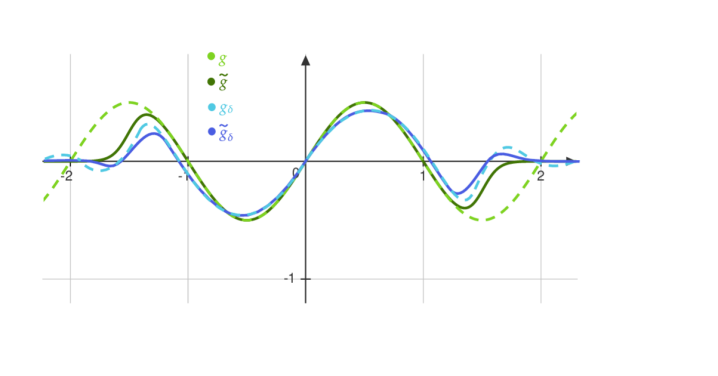
Figure 5. Visualization of the cutoffs and approximations in the first step of the proof of Theorem 6.16 for $C=2$. We start with a function $g$, which is first multiplied by the cutoff-function $\Psi_{C}$, giving $\tilde{g}$. This function is then approximated by a polynomial $g_{\delta}$. Multiplying $g_{\delta}$ by the cutoff function $\Psi_{C}$ results in a function which is here called $\tilde{g}_{\delta}$ (but does not directly appear in the proof). The function $\tilde{f}_{\delta}$ is then given by the difference between $\tilde{g}$ and $\tilde{g}_{\delta}$.

This gives

$$\big{\|}f_{\delta}\big{(}\chi_{\Lambda}\>\mathrm{Op}_{\alpha}(\mathfrak{a}_{0,1}\big{)}\>\chi_{\Lambda}\big{)}-\chi_{\Lambda}\>f_{\delta}\big{(}\mathrm{Op}_{\alpha}(\mathfrak{a}_{0,1})\big{)}\>\chi_{\Lambda}\big{\|}_{1}$$

$$=\big{\|}\tilde{f}_{\delta}\big{(}\chi_{\Lambda}\>\mathrm{Op}_{\alpha}(\mathfrak{a}_{0,1})\>\chi_{\Lambda}\big{)}-\chi_{\Lambda}\>\tilde{f}_{\delta}\big{(}\mathrm{Op}_{\alpha}(\mathfrak{a}_{0,1})\big{)}\>\chi_{\Lambda}\big{\|}_{1}$$

$$\leq c(C)\>\delta\>\big{\|}\chi_{\Lambda}\>\mathrm{Op}_{\alpha}(\mathfrak{a}_{0,1})\>(1-\chi_{\Lambda})\big{\|}_{\sigma}^{\sigma}\>.$$

In order to further estimate the last norm, recall that by definition of the symbol $a$ we have

$$\chi_{\Lambda}\>\mathrm{Op}_{\alpha}(\mathfrak{a}_{0,1})=\chi_{\Lambda}\>\mathrm{Op}_{\alpha}\big{(}I_{\Omega}\,a\big{)}\>.$$

Moreover, using Lemma 5.5 we obtain

$$\chi_{\Lambda}\mathrm{Op}_{\alpha}\big{(}I_{\Omega}\,a\big{)}=\chi_{\Lambda}\mathrm{Op}_{\alpha}(a)\>P_{\Omega,\alpha}\>.$$

Therefore, also applying Lemma 6.15 with $q=\sigma$, we conclude that for $\alpha$ large enough

$$\big{\|}f_{\delta}\big{(}\chi_{\Lambda}\>\mathrm{Op}_{\alpha}(\mathfrak{a}_{0,1})\>\chi_{\Lambda}\big{)}-\chi_{\Lambda}\>f_{\delta}(\mathrm{Op}_{\alpha}(\mathfrak{a}_{0,1}))\>\chi_{\Lambda}\big{\|}_{1}$$

$$\leq c(C)\>\delta\>\big{\|}\chi_{\Lambda}\>\mathrm{Op}_{\alpha}(a)\>P_{\alpha,\Omega}\>(1-\chi_{\Lambda})\big{\|}_{\sigma}^{\sigma}\leq c_{\sigma,M,\rho,C}\>\delta\>\ln\alpha\>,$$

(with a constant $c_{q,M,\rho,C}$ depending on $\sigma,M,\rho$ and $C$). Using this inequality, we can estimate the trace by

$$\operatorname{tr}D_{\alpha}(g,\Lambda,\mathfrak{a}_{0,1})\leq \operatorname{tr}D_{\alpha}(g_{\delta},\Lambda,\mathfrak{a}_{0,1})+\|D_{\alpha}(f_{\delta},\Lambda,\mathfrak{a}_{0,1})\|_{1}$$

$$\leq \operatorname{tr}D_{\alpha}(g_{\delta},\Lambda,\mathfrak{a}_{0,1})+c_{C,\sigma,M,\rho}\>\delta\>\ln\alpha\>.$$

In order to compute the remaining trace, we can again apply Theorem 6.3 (exactly as in the example (6.4)). This gives

$$\operatorname{tr}D_{\alpha}(g_{\delta},\Lambda,\mathfrak{a}_{0,1})=\frac{1}{2\pi^{2}}\ln(\alpha)\>U(1;g_{\delta})+\mathcal{O}(1)\>,$$

and thus

$$\operatorname{tr}D_{\alpha}(g,\Lambda,\mathfrak{a}_{0,1})\leq\frac{1}{2\pi^{2}}\>\ln(\alpha)\>U(1;g_{\delta})+c_{\sigma,M,\rho,C}\>\delta\>\ln\alpha+\mathcal{O}(1)\>,$$

which yields

$$\limsup\limits_{\alpha\rightarrow\infty}\frac{1}{\ln\alpha}\operatorname{tr}D_{\alpha}(g,\Lambda,\mathfrak{a}_{0,1})\leq\frac{1}{2\pi^{2}}U(1;g_{\delta})+c_{\sigma,M,\rho,C}\>\delta\>.$$ (6.10)

In the next step we want to take the limit $\delta\rightarrow 0$. To this end, we need to analyze how the quantity $U(1;g_{\delta})$ behaves in this limit. In particular, we want to show that

$$\lim\limits_{\delta\rightarrow 0}U(1;g_{\delta})=U(1;g)\>.$$

Thus we begin by estimating

$$\big{|}U(1;g_{\delta})-U(1;g)\big{|}=\big{|}U(1;f_{\delta})\big{|}$$

$$\leq\underbrace{\left|\int_{0}^{1/2}\frac{1}{t(1-t)}\big{(}f_{\delta}(t)-tf_{\delta}(1)\big{)}dt\right|}_{\text{(I)}}+\underbrace{\left|\int_{1/2}^{1}\frac{1}{t(1-t)}\big{(}f_{\delta}(t)-tf_{\delta}(1)\big{)}dt\right|}_{\text{(II)}}\>.$$

For the estimate of $(I)$ consider the Taylor expansion for $f_{\delta}$ around $t=0$ keeping in mind that $f_{\delta}(0)=0$:

$$f_{\delta}(t)=tf_{\delta}^{\prime}(0)+\frac{t^{2}}{2}f_{\delta}^{\prime\prime}\big{(}\tilde{t}\big{)}\qquad\text{for suitable~{}$\tilde{t}\in[0,t]$}\>,$$

and therefore

$$\text{(I)}\leq\int_{0}^{1/2}\underbrace{\Big{|}\frac{1}{(1-t)}\Big{|}}_{\leq 2}\Big{(}\underbrace{|f_{\delta}^{\prime}(0)|}_{\leq\delta}+\underbrace{|t/2|}_{\leq 1/4}\underbrace{|f_{\delta}^{\prime\prime}(\tilde{t})|}_{\leq\delta}\Big{)}dt+\int_{0}^{1/2}\underbrace{\Big{|}\frac{1}{(1-t)}\Big{|}}_{\leq 2}\underbrace{|f_{\delta}(1)|}_{\leq\delta}dt\leq\frac{9}{4}\>\delta$$

(note that $\tilde{t}$ is actually a function of $t$, but this is unproblematic because $f_{\delta}^{\prime\prime}$ is uniformly bounded).

Similarly, for the estimate of (II) we use the Taylor expansion of $f_{\delta}$, but now around $t=1$,

$$f_{\delta}(t)=f_{\delta}(1)+(t-1)f_{\delta}^{\prime}(1)+\frac{(t-1)^{2}}{2}f_{\delta}^{\prime\prime}(\tilde{t})\qquad\text{for suitable~{}$\tilde{t}\in[0,t]$}\>.$$

We thus obtain

(II) $$\leq\int_{1/2}^{1}\Big{|}\frac{1}{t(1-t)}\Big{|}\Big{(}|1-t|\>|f_{\delta}(1)|+|1-t|\>|f_{\delta}^{\prime}(1)|+\frac{|1-t|^{2}}{2}|f_{\delta}^{\prime\prime}(\tilde{t})|\Big{)}\>dt$$

$$\leq \int_{1/2}^{1}\underbrace{|1/t|}_{\leq 2}\Big{(}\underbrace{|f_{\delta}(1)|}_{\leq\delta}+\underbrace{|f_{\delta}^{\prime}(1)|}_{\leq\delta}+\underbrace{\frac{|1-t|}{2}}_{\leq 1/4}\underbrace{|f_{\delta}^{\prime\prime}(\tilde{t})|}_{\leq\delta}\Big{)}\>dt\leq\frac{9}{4}\delta\>.$$

Therefore, taking the limit $\delta\rightarrow 0$ in (6.10) gives

$$\limsup\limits_{\alpha\rightarrow\infty}\frac{1}{\ln\alpha}\operatorname{tr}D_{\alpha}(g,\Lambda,\mathfrak{a}_{0,1})\leq\frac{1}{2\pi^{2}}\>U(1;g)\>.$$

Analogously, using

$$\frac{1}{2\pi^{2}}\ln(\alpha)\>U(1;g_{\delta})+\mathcal{O}(1) =\operatorname{tr}D_{\alpha}(g_{\delta},\Lambda,\mathfrak{a}_{0,1})\leq\operatorname{tr}D_{\alpha}(g,\Lambda,\mathfrak{a}_{0,1})+\|D_{\alpha}(f_{\delta},\Lambda,\mathfrak{a}_{0,1})\|_{1}$$

$$\leq\operatorname{tr}D_{\alpha}(g,\Lambda,\mathfrak{a}_{0,1})+c_{q,M,\rho,C}\>\delta\>\ln\alpha\>,$$

we obtain

$$\liminf\limits_{\alpha\rightarrow\infty}\frac{1}{\ln\alpha}\operatorname{tr}D_{\alpha}(g,\Lambda,\mathfrak{a}_{0,1})\geq\frac{1}{2\pi^{2}}\>U(1;g_{\delta})+c_{q,M,\rho,C}\>\delta\>.$$

Now we can take the limit $\delta\rightarrow 0$,

$$\liminf\limits_{\alpha\rightarrow\infty}\frac{1}{\ln\alpha}\operatorname{tr}D_{\alpha}(g,\Lambda,\mathfrak{a}_{0,1})\geq\frac{1}{2\pi^{2}}\>U(1;g)\>.$$

Combining the inequalities for the $\limsup$ and $\liminf$, we conclude that for any $g\in C^{2}(\mathbb{R})$,

$$\lim\limits_{\alpha\rightarrow\infty}\frac{1}{\ln\alpha}\operatorname{tr}D_{\alpha}(g,\Lambda,\mathfrak{a}_{0,1})=\frac{1}{2\pi^{2}}\>U(1;g)\>.$$ (6.11)

Second Step: Proof for $g$ as in claim.
By choosing a suitable partition of unity and making use of linearity, it suffices to consider the case $X=\{z\}$ meaning that $g$ is non-differentiable only at one point $z$. Next we decompose $g$ into two parts with a cutoff function $\xi\in C^{\infty}_{0}(\mathbb{R})$ with the property that

$$\xi(t)=\begin{cases}1,\quad|t|\leq 1/2\\ 0,\quad|t|\geq 1\end{cases}\>.$$

and writing

$$g=g_{R}^{(1)}+g_{R}^{(2)}\>,$$

with

$$\begin{aligned} g_{R}^{(1)}(t)&:=g(t)\>\xi\big{(}(t-z)/R\big{)}\quad&&\Rightarrow\quad\operatorname{supp}g_{R}^{(1)}\subseteq[z-R,z+R]\>,\\ g_{R}^{(2)}(t)&:=g(t)-g_{R}^{(1)}(t)\quad&&\Rightarrow\quad\operatorname{supp}g_{R}^{(2)}\subseteq[-C,C]\>;\end{aligned}$$

see also Figure 6.

Figure 6. Schematic plot of a function $g$ (blue) which is non-differentiable at $z=0$ with the corresponding functions $g^{(1)}_{1/2}$ (red), $g^{(1)}_{1/4}$ (orange) and $g^{(1)}_{1/10}$ (green): They are cutting out the non-differentiable point.

Note that the derivatives of $g_{R}^{(1)}$ satisfy the bounds

$$\Big{(}g_{R}^{(1)}\Big{)}^{(k)}(t)=\sum_{n=0}^{k}\>c(n,k)\>g^{(k-n)}(t)\>\xi^{(n)}\big{(}(t-z)/R\big{)}\>\frac{1}{R^{n}}\>,$$

(with some numerical constants $c(n,k)$) and therefore the norm ${\,\vrule depth=3.0pt,height=9.0pt}{\vrule depth=3.0pt,height=9.0pt}{\vrule depth=3.0pt,height=9.0pt}{\vrule depth=3.0pt,height=9.0pt}\,.{\,\vrule depth=3.0pt,height=9.0pt}{\vrule depth=3.0pt,height=9.0pt}{\vrule depth=3.0pt,height=9.0pt}{\vrule depth=3.0pt,height=9.0pt}\,_{2}$ in Lemma 6.8 can be estimated by

$${\,\vrule depth=3.0pt,height=9.0pt}{\vrule depth=3.0pt,height=9.0pt}{\vrule depth=3.0pt,height=9.0pt}{\vrule depth=3.0pt,height=9.0pt}\,g_{R}^{(1)}{\,\vrule depth=3.0pt,height=9.0pt}{\vrule depth=3.0pt,height=9.0pt}{\vrule depth=3.0pt,height=9.0pt}{\vrule depth=3.0pt,height=9.0pt}\,_{2} =\max_{0\leq k\leq 2}\;\sup_{t\neq z}\bigg{|}\sum_{n=0}^{k}c(n,k)\>g^{(k-n)}(t)\>\xi^{(n)}\big{(}(t-z)/R\big{)}\>\frac{1}{R^{n}}\bigg{|}\cdot|t-z|^{-\gamma+k}$$

$$\leq\max_{0\leq k\leq 2}\;\sup_{t\neq z}\sum_{n=0}^{k}\big{|}c(n,k)\big{|}\>\big{|}g^{(k-n)}(t)\big{|}\>|t-z|^{-\gamma+k-n}\>\big{|}\xi^{(n)}\big{(}(t-z)/R\big{)}\big{|}\>\frac{|t-z|^{n}}{R^{n}}\>.$$

Noting that on the support of $\big{(}g_{R}^{(1)}\big{)}^{(k)}$ we have

$$\frac{|t-z|}{R}\leq 1\>,$$

we conclude that

$${\,\vrule depth=3.0pt,height=9.0pt}{\vrule depth=3.0pt,height=9.0pt}{\vrule depth=3.0pt,height=9.0pt}{\vrule depth=3.0pt,height=9.0pt}\,g_{R}^{(1)}{\,\vrule depth=3.0pt,height=9.0pt}{\vrule depth=3.0pt,height=9.0pt}{\vrule depth=3.0pt,height=9.0pt}{\vrule depth=3.0pt,height=9.0pt}\,_{2}\leq c{\,\vrule depth=3.0pt,height=9.0pt}{\vrule depth=3.0pt,height=9.0pt}{\vrule depth=3.0pt,height=9.0pt}{\vrule depth=3.0pt,height=9.0pt}\,g{\,\vrule depth=3.0pt,height=9.0pt}{\vrule depth=3.0pt,height=9.0pt}{\vrule depth=3.0pt,height=9.0pt}{\vrule depth=3.0pt,height=9.0pt}\,_{2}$$

with $c$ independent of $R$ (also note that ${\,\vrule depth=3.0pt,height=9.0pt}{\vrule depth=3.0pt,height=9.0pt}{\vrule depth=3.0pt,height=9.0pt}{\vrule depth=3.0pt,height=9.0pt}\,g{\,\vrule depth=3.0pt,height=9.0pt}{\vrule depth=3.0pt,height=9.0pt}{\vrule depth=3.0pt,height=9.0pt}{\vrule depth=3.0pt,height=9.0pt}\,_{2}$ is bounded by assumption).

For what follows, it is also useful to keep in mind that

$$0=g_{R}^{(1)}(0)=g_{R}^{(1)}(1)=g_{R}^{(2)}(0)=g_{R}^{(2)}(1)\>.$$

Now we apply (6.11) to the function $g_{R}^{(2)}$ (which clearly is in $C^{(2)}(\mathbb{R})$),

$$\lim\limits_{\alpha\rightarrow\infty}\frac{1}{\ln\alpha}\operatorname{tr}D_{\alpha}(g_{R}^{(2)},\Lambda,\mathfrak{a}_{0,1})=U(1;g_{R}^{(2)})\>.$$

Next, we apply Lemma 6.8 to $g_{R}^{(1)}$ with $A$ and $P$ as before and some $\sigma\in(0,1)$ with $\sigma<\gamma$,

$$\big{\|}D_{\alpha}\big{(}g_{R}{(1)},\Lambda,\mathfrak{a}_{0,1}\big{)}\big{\|}_{1}\leq C_{\sigma}{\,\vrule depth=3.0pt,height=9.0pt}{\vrule depth=3.0pt,height=9.0pt}{\vrule depth=3.0pt,height=9.0pt}{\vrule depth=3.0pt,height=9.0pt}\,g{\,\vrule depth=3.0pt,height=9.0pt}{\vrule depth=3.0pt,height=9.0pt}{\vrule depth=3.0pt,height=9.0pt}{\vrule depth=3.0pt,height=9.0pt}\,_{2}\>R^{\gamma-\sigma}\>\big{\|}\chi_{\Lambda}\>\mathrm{Op}_{\alpha}(a)\>P_{\Omega,\alpha}\>(1-\chi_{\Lambda})\big{\|}_{\sigma}^{\sigma}\>.$$

Applying Lemma 6.15 (for $\alpha$ large enough) with $q=\sigma$ yields

$$\big{\|}D_{\alpha}\big{(}g_{R}{(1)},\Lambda,\mathfrak{a}_{0,1}\big{)}\big{\|}_{1}\leq{\,\vrule depth=3.0pt,height=9.0pt}{\vrule depth=3.0pt,height=9.0pt}{\vrule depth=3.0pt,height=9.0pt}{\vrule depth=3.0pt,height=9.0pt}\,g{\,\vrule depth=3.0pt,height=9.0pt}{\vrule depth=3.0pt,height=9.0pt}{\vrule depth=3.0pt,height=9.0pt}{\vrule depth=3.0pt,height=9.0pt}\,_{2}\>C_{\sigma,M,\rho\>}R^{\gamma-\sigma}\ln\alpha\>.$$

Just as before, it follows that

$$\limsup\limits_{\alpha\rightarrow\infty}\frac{1}{\ln\alpha}\operatorname{tr}D_{\alpha}(g,\Lambda,\mathfrak{a}_{0,1}) \leq U\big{(}1;g_{R}^{(2)}\big{)}+{\,\vrule depth=3.0pt,height=9.0pt}{\vrule depth=3.0pt,height=9.0pt}{\vrule depth=3.0pt,height=9.0pt}{\vrule depth=3.0pt,height=9.0pt}\,g{\,\vrule depth=3.0pt,height=9.0pt}{\vrule depth=3.0pt,height=9.0pt}{\vrule depth=3.0pt,height=9.0pt}{\vrule depth=3.0pt,height=9.0pt}\,_{2}\>C_{\sigma,M,\rho}\>R^{\gamma-\sigma}$$

$$\liminf\limits_{\alpha\rightarrow\infty}\frac{1}{\ln\alpha}\operatorname{tr}D_{\alpha}(g,\Lambda,\mathfrak{a}_{0,1}) \geq U\big{(}1;g_{R}^{(2)}\big{)}+{\,\vrule depth=3.0pt,height=9.0pt}{\vrule depth=3.0pt,height=9.0pt}{\vrule depth=3.0pt,height=9.0pt}{\vrule depth=3.0pt,height=9.0pt}\,g{\,\vrule depth=3.0pt,height=9.0pt}{\vrule depth=3.0pt,height=9.0pt}{\vrule depth=3.0pt,height=9.0pt}{\vrule depth=3.0pt,height=9.0pt}\,_{2}\>C_{\sigma,M,\rho}\>R^{\gamma-\sigma}\>.$$

The end result follows just as before by taking the limit $R\rightarrow 0$, provided that we can show the convergence $U(1;g_{R}^{(2)})\rightarrow U(1;g)$ for $R\rightarrow 0$. To this end we need to estimate the function

$$U\big{(}1;g-g_{R}^{(2)}\big{)}=U(1;g_{R}^{(1)})=\underbrace{\int_{0}^{1/2}\frac{1}{t(1-t)}\>g_{R}^{(1)}(t)\>dt}_{\text{(i)}}+\underbrace{\int_{1/2}^{1}\frac{1}{t(1-t)}\>g_{R}^{(1)}(t)\>dt}_{\text{(ii)}}\>.$$

We first note that, unless $z=0$ or $z=1$, both integrals are bounded by

$$|\text{(i)}|\leq cR\>,\quad|\text{(ii)}|\leq cR\>,$$

for $R$ sufficiently small (more precisely, so small that $g_{R}^{(1)}$ vanishes in neighborhoods around $0$ and $1$; note that the integrand is supported in $[z-R,z+R]$ and bounded uniformly in $R$). These estimates show that $\lim_{R\rightarrow 0}U(1;g-g_{R}^{(2)})=0$ in the case that $z$ is neither $0$ nor $1$. It remains to consider the cases $z=0$ and $z=1$:

• Case $z=0$: First note that

  $$|g_{R}^{(1)}(t)|\leq{\,\vrule depth=3.0pt,height=9.0pt}{\vrule depth=3.0pt,height=9.0pt}{\vrule depth=3.0pt,height=9.0pt}{\vrule depth=3.0pt,height=9.0pt}\,g_{R}^{(1)}{\,\vrule depth=3.0pt,height=9.0pt}{\vrule depth=3.0pt,height=9.0pt}{\vrule depth=3.0pt,height=9.0pt}{\vrule depth=3.0pt,height=9.0pt}\,_{2}|t|^{\gamma}\leq c{\,\vrule depth=3.0pt,height=9.0pt}{\vrule depth=3.0pt,height=9.0pt}{\vrule depth=3.0pt,height=9.0pt}{\vrule depth=3.0pt,height=9.0pt}\,g{\,\vrule depth=3.0pt,height=9.0pt}{\vrule depth=3.0pt,height=9.0pt}{\vrule depth=3.0pt,height=9.0pt}{\vrule depth=3.0pt,height=9.0pt}\,_{2}|t|^{\gamma}\>,$$

  where c is again independent of $R$. This yields for $R\leq 1/2$,

  $$|\text{(i)}| =\Big{|}\int_{0}^{1/2}\frac{1}{t(1-t)}g_{R}^{(1)}(t)dt\Big{|}\leq c\int_{0}^{R}\underbrace{\frac{1}{|1-t|}}_{\leq 1/(1-R)}{\,\vrule depth=3.0pt,height=9.0pt}{\vrule depth=3.0pt,height=9.0pt}{\vrule depth=3.0pt,height=9.0pt}{\vrule depth=3.0pt,height=9.0pt}\,g{\,\vrule depth=3.0pt,height=9.0pt}{\vrule depth=3.0pt,height=9.0pt}{\vrule depth=3.0pt,height=9.0pt}{\vrule depth=3.0pt,height=9.0pt}\,_{2}|t|^{\gamma-1}dt$$

  $$\leq\frac{c}{1-R}{\,\vrule depth=3.0pt,height=9.0pt}{\vrule depth=3.0pt,height=9.0pt}{\vrule depth=3.0pt,height=9.0pt}{\vrule depth=3.0pt,height=9.0pt}\,g{\,\vrule depth=3.0pt,height=9.0pt}{\vrule depth=3.0pt,height=9.0pt}{\vrule depth=3.0pt,height=9.0pt}{\vrule depth=3.0pt,height=9.0pt}\,_{2}\underbrace{\int_{0}^{R}|t|^{\gamma-1}}_{=R^{\gamma}/\gamma}dt\leq c{\,\vrule depth=3.0pt,height=9.0pt}{\vrule depth=3.0pt,height=9.0pt}{\vrule depth=3.0pt,height=9.0pt}{\vrule depth=3.0pt,height=9.0pt}\,g{\,\vrule depth=3.0pt,height=9.0pt}{\vrule depth=3.0pt,height=9.0pt}{\vrule depth=3.0pt,height=9.0pt}{\vrule depth=3.0pt,height=9.0pt}\,_{2}\frac{R^{\gamma}}{\gamma(1-R)}\>,$$

  which vanishes in the limit $R\rightarrow 0$. Moreover, the integral (ii) vanishes for $R<1/2$.

• Case $z=1$: Similarly as in the previous case, we now have

  $$\text{(i)}=0\qquad\text{for~{}$R<1/2$}\>.$$

  Moreover, just as in the previous case, one can estimate

  $$|g_{R}^{(1)}(t)|\leq c{\,\vrule depth=3.0pt,height=9.0pt}{\vrule depth=3.0pt,height=9.0pt}{\vrule depth=3.0pt,height=9.0pt}{\vrule depth=3.0pt,height=9.0pt}\,g{\,\vrule depth=3.0pt,height=9.0pt}{\vrule depth=3.0pt,height=9.0pt}{\vrule depth=3.0pt,height=9.0pt}{\vrule depth=3.0pt,height=9.0pt}\,_{2}|1-t|^{\gamma}\>,$$

  for any $t\in(1/2,1)$ and with $c$ independent of $R$. This yields for $R\leq 1/2$

  $$|\text{(ii)}|\leq c\,{\,\vrule depth=3.0pt,height=9.0pt}{\vrule depth=3.0pt,height=9.0pt}{\vrule depth=3.0pt,height=9.0pt}{\vrule depth=3.0pt,height=9.0pt}\,g{\,\vrule depth=3.0pt,height=9.0pt}{\vrule depth=3.0pt,height=9.0pt}{\vrule depth=3.0pt,height=9.0pt}{\vrule depth=3.0pt,height=9.0pt}\,_{2}\int_{1-R}^{1}\frac{1}{|t|}\>|1-t|^{1-\gamma}\>dt\leq c\,{\,\vrule depth=3.0pt,height=9.0pt}{\vrule depth=3.0pt,height=9.0pt}{\vrule depth=3.0pt,height=9.0pt}{\vrule depth=3.0pt,height=9.0pt}\,g{\,\vrule depth=3.0pt,height=9.0pt}{\vrule depth=3.0pt,height=9.0pt}{\vrule depth=3.0pt,height=9.0pt}{\vrule depth=3.0pt,height=9.0pt}\,_{2}\>\frac{R^{\gamma}}{\gamma(1-R)}\>,$$

  which again vanishes for $R\rightarrow 0$.

This concludes the proof. ∎

We finally apply Theorem 6.16 to the function $\eta$ and the matrix- valued symbol $\mathfrak{A}_{0}$ (see (2.1) and (4.4)).

Corollary 6.18.

For $\eta$, $\Lambda$ and $\mathfrak{A}_{0}$ as before,

$$\lim\limits_{\alpha\rightarrow\infty}\lim\limits_{u_{0}\rightarrow\infty}\frac{1}{\ln\alpha}\operatorname{tr}D_{\alpha}(\eta,\Lambda,\mathfrak{A}_{0})=\frac{1}{3}\>.$$

Proof.

Combining Theorem 6.16 with Lemma 6.17 (and the fact that $\eta(1)=\eta(0)=0$), we obtain

$$\lim\limits_{\alpha\rightarrow\infty}\lim\limits_{u_{0}\rightarrow\infty}\frac{1}{\ln\alpha}\operatorname{tr}D_{\alpha}(\eta,\Lambda,\mathfrak{a}_{0,1})=\frac{1}{2\pi^{2}}U(1;\eta)\>.$$

Evaluating $U(1;\eta)$, an elementary computation yields

$$U(1;\eta)=\int_{0}^{1}\frac{-x\ln(x)-(1-x)\ln(1-x)}{t(1-t)}\>dt=\frac{\pi^{2}}{3}\>,$$

and therefore

$$\lim\limits_{\alpha\rightarrow\infty}\lim\limits_{u_{0}\rightarrow\infty}\frac{1}{\ln\alpha}\operatorname{tr}D_{\alpha}(\eta,\Lambda,\mathfrak{a}_{0,1})=\frac{1}{6}\>.$$

Repeating the procedure analogously for $\mathfrak{a}_{0,2}$ gives

$$\lim\limits_{\alpha\rightarrow\infty}\lim\limits_{u_{0}\rightarrow\infty}\frac{1}{\ln\alpha}\operatorname{tr}D_{\alpha}(\eta,\Lambda,\mathfrak{a}_{0,2})=\frac{1}{6}\>,$$

and therefore

$$\lim\limits_{\alpha\rightarrow\infty}\lim\limits_{u_{0}\rightarrow\infty}\frac{1}{\ln\alpha}\operatorname{tr}D_{\alpha}(\eta,\Lambda,\mathfrak{A}_{0})=\frac{1}{3}\>.$$

This gives the result. ∎

Corollary 6.18 already looks quite similar to Theorem 1.1. The remaining task is to show equality in (4.3). To this end, we need to show that all the correction terms drop out in the limits $u_{0}\rightarrow\infty$ and $\alpha\rightarrow\infty$. The next section is devoted to this task.

7. Estimating the Error Terms

In the previous section, we worked with the simplified kernel (4.4) and computed the corresponding entropy. In this section, we estimate all the errors, thereby proving the equality in (4.3). Our procedure is summarized as follows. Using (3.12), the regularized projection operator $(\Pi_{\varepsilon}^{-})_{kn}$ can be written as

$$(\Pi_{\varepsilon}^{-})_{kn}=\mathrm{op}_{\alpha}\big{(}2\>(A_{\varepsilon}+\mathcal{R}_{\varepsilon,0})\big{)}$$

and $A_{\varepsilon}$ as in (3.13) and the error term

$$\mathcal{R}_{\varepsilon,0}(u,u^{\prime},\xi):=\mathcal{R}_{0}(u,u^{\prime},M\xi/\varepsilon)\>,$$

We denote the corresponding symbol by

$$\big{(}(a_{\mathrm{full}})_{ij}\big{)}_{1\leq i,j\leq 2}:=A_{\mathrm{full}}:=2(A_{\varepsilon}+\mathcal{R}_{\varepsilon,0})\>.$$

In preparation, translate $\Lambda$ to $\Lambda_{0}$ with the help of the unitary operator $T_{u_{0}}$ making use of Lemma 5.2. Moreover, we use that the operators $(\Pi_{\varepsilon}^{-})_{kn}$ and $\mathrm{Op}_{\alpha}(\mathfrak{A}_{0})$ are self-adjoint. We thus obtain

$$d_{\alpha}(\eta,\Lambda,A_{\mathrm{full}})-D_{\alpha}(\eta,\Lambda,\mathfrak{A}_{0})=d_{\alpha}(\eta,\Lambda_{0},T_{u_{0}}(A_{\mathrm{full}}))-D_{\alpha}(\eta,\Lambda_{0},T_{u_{0}}(\mathfrak{A}_{0}))\>,$$

where $\mathfrak{A}_{0}$ is the kernel of the limiting operator from (4.4). Now we can estimate

$$\|d_{\alpha}(\eta,\Lambda_{0},T_{u_{0}}(A_{\mathrm{full}}))-D_{\alpha}(\eta,\Lambda_{0},T_{u_{0}}(\mathfrak{A}_{0}))\|_{1}$$

$$\leq\Big{\|}\eta\big{(}\chi_{\Lambda_{0}}\>\mathrm{Op}_{\alpha}(T_{u_{0}}(A_{\mathrm{full}}))\>\chi_{\Lambda_{0}}\big{)}-\eta\big{(}\chi_{\Lambda_{0}}\>\mathrm{Op}_{\alpha}(T_{u_{0}}(\mathfrak{A}_{0})))\>\chi_{\Lambda_{0}}\big{)}\Big{\|}_{1}$$ (I)

$$\quad\>+\Big{\|}\chi_{\Lambda_{0}}\>\big{(}\eta\left(\mathrm{Op}_{\alpha}\big{(}T_{u_{0}}(A_{\mathrm{full}})\big{)}\right)-\eta\left(\mathrm{Op}_{\alpha}\big{(}T_{u_{0}}(\mathfrak{A}_{0})\big{)}\right)\big{)}\>\chi_{\Lambda_{0}}\Big{\|}_{1}\>.$$ (II)

In the following we will estimate the expressions (I) and (II) separately.

7.1. Estimate of the Error Term (I)

We begin with the following simplified result from [26], which is related to Lemma 6.8.

Theorem 7.1.

[26, Condition 2.3 and Theorem 2.4 (simplified to our needs)] Let $f\in C^{n}(\mathbb{R}\setminus\{x_{0}\})\cap C(\mathbb{R})$ with some $x_{0}\in\mathbb{R}$ and $n\geq 2$ be a function such that $\operatorname{supp}f=[x_{0}-R,x_{0}+R]$ for some $R>0$ and

$${\,\vrule depth=3.0pt,height=9.0pt}{\vrule depth=3.0pt,height=9.0pt}{\vrule depth=3.0pt,height=9.0pt}{\vrule depth=3.0pt,height=9.0pt}\,f{\,\vrule depth=3.0pt,height=9.0pt}{\vrule depth=3.0pt,height=9.0pt}{\vrule depth=3.0pt,height=9.0pt}{\vrule depth=3.0pt,height=9.0pt}\,_{n}=\max_{0\leq k\leq n}\sup_{x\neq x_{0}}\big{|}f^{(k)}(x)\big{|}|x-x_{0}|^{-\gamma+k}<\infty\>,$$

with some $\gamma>0$. Let $\mathfrak{S}$ be a $q$-normed ideal of compact operators on $\mathfrak{H}$ such that there is a $\sigma\in(0,1]$ with $\sigma<\gamma$ and

$$(n-\sigma)^{-1}<q\leq 1\>.$$

Let $A,B$ be two bounded self-adjoint operators on $\mathfrak{H}$. Suppose that $|A-B|^{\sigma}\in\mathfrak{S}$, then

$$\|f(A)-f(B)\|_{\mathfrak{S}}\leq C_{n}\>R^{\gamma-\sigma}\>{\,\vrule depth=3.0pt,height=9.0pt}{\vrule depth=3.0pt,height=9.0pt}{\vrule depth=3.0pt,height=9.0pt}{\vrule depth=3.0pt,height=9.0pt}\,f{\,\vrule depth=3.0pt,height=9.0pt}{\vrule depth=3.0pt,height=9.0pt}{\vrule depth=3.0pt,height=9.0pt}{\vrule depth=3.0pt,height=9.0pt}\,_{n}\>\big{\|}|A-B|^{\sigma}\big{\|}_{\mathfrak{S}}$$

with a positive constant $C_{n}$ independent of $A,B,f$ and $R$.

In order to apply this theorem to the function $\eta$, as in the proof of Theorem 6.16 we use a partition of unity. Similar as in Lemma 6.17, we need to choose $\gamma<1$. This gives rise to the constraint

$$\sigma<1\>.$$

With this in mind, we choose $\sigma$ as a fixed number smaller than but close to one. In particular, it is useful to choose sigma as some fixed number in the range

$$\sigma\in\Big{(}\frac{2}{3}\>,\>1\Big{)}\>.$$

Setting $A=\chi_{\Lambda_{0}}\mathrm{Op}_{\alpha}(T_{u_{0}}(A_{\mathrm{full}}))\chi_{\Lambda_{0}}$ and $B=\chi_{\Lambda_{0}}\mathrm{Op}_{\alpha}(T_{u_{0}}(\mathfrak{A}_{0}))\chi_{\Lambda_{0}}$ (which are clearly bounded and self-adjoint) we obtain

$$\begin{split}&\big{\|}\eta\big{(}\chi_{\Lambda_{0}}\>\mathrm{Op}_{\alpha}\big{(}T_{u_{0}}(A_{\mathrm{full}})\big{)}\>\chi_{\Lambda_{0}}\big{)}-\eta\big{(}\chi_{\Lambda_{0}}\mathrm{Op}_{\alpha}\big{(}T_{u_{0}}(\mathfrak{A}_{0})\big{)}\chi_{\Lambda_{0}}\big{)}\big{\|}_{1}\\ &\leq C\>\big{\|}\chi_{\Lambda_{0}}\>\mathrm{Op}_{\alpha}\big{(}T_{u_{0}}(A_{\mathrm{full}})-T_{u_{0}}(\mathfrak{A}_{0})\big{)}\>\chi_{\Lambda_{0}}\big{\|}_{\sigma}^{\sigma}\end{split}$$ (7.1)

with C independent of $A$ and $B$ (and thus in particular independent of $u_{0}$ and $\alpha$).

For ease of notation, from now on we will denote

$$\big{(}\Delta(a_{ij})_{u_{0}}\big{)}_{1\leq i,j,\leq 2}:=\Delta A_{u_{0}}:=T_{u_{0}}(A_{\mathrm{full}})-T_{u_{0}}(\mathfrak{A}_{0})\>.$$

Note that the symbol of the $\mathrm{Op}_{\alpha}(.)$ in (7.1) is matrix-valued. Since most estimates for such operators have been carried out for scalar-valued symbols, we now show how to reduce our case to a problem with scalar-valued symbols. To this end, we use the $\sigma$-triangle inequality of $\|.\|_{\sigma}$ in the following way,

$$\|\chi_{\Lambda_{0}}\mathrm{Op}_{\alpha}(\Delta A_{u_{0}})\chi_{\Lambda_{0}}\|_{\sigma}^{\sigma}$$

$$\leq C\>\Big{\|}\chi_{\Lambda_{0}}\mathrm{Op}_{\alpha}\left(\begin{pmatrix}\Delta(a_{11})_{u_{0}}&0\\ 0&0\end{pmatrix}\right)\chi_{\Lambda_{0}}\Big{\|}_{\sigma}^{\sigma}+C\>\Big{\|}\chi_{\Lambda_{0}}\mathrm{Op}_{\alpha}\left(\begin{pmatrix}0&\Delta(a_{12})_{u_{0}}\\ 0&0\end{pmatrix}\right)\chi_{\Lambda_{0}}\Big{\|}_{\sigma}^{\sigma}$$

$$\quad\>+C\>\Big{\|}\chi_{\Lambda_{0}}\mathrm{Op}_{\alpha}\left(\begin{pmatrix}0&0\\ \Delta(a_{21})_{u_{0}}&0\end{pmatrix}\right)\chi_{\Lambda_{0}}\Big{\|}_{\sigma}^{\sigma}+C\>\Big{\|}\chi_{\Lambda_{0}}\mathrm{Op}_{\alpha}\left(\begin{pmatrix}0&0\\ 0&\Delta(a_{22})_{u_{0}}\end{pmatrix}\right)\chi_{\Lambda_{0}}\Big{\|}_{\sigma}^{\sigma}\>,$$

with a constant $C>0$ only depending on $\sigma$. For the next step, recall that for any operator $A$ its Schatten-norm $\|A\|_{\sigma}$ only depends on the singular values of $A^{*}A$. Considering a matrix $A$ with only one non-zero entry $a$, the non-zero singular values of $A^{*}A$ are the same as those of $a^{*}a$. Applying this to the estimate from before, we obtain

$$\big{\|}\chi_{\Lambda_{0}}\mathrm{Op}_{\alpha}(\Delta A_{u_{0}})\chi_{\Lambda_{0}}\big{\|}_{\sigma}^{\sigma}\leq C\sum_{i,j=1}^{2}\Big{\|}\chi_{\Lambda_{0}}\>\mathrm{Op}_{\alpha}\big{(}\Delta(a_{ij})_{u_{0}}\big{)}\>\chi_{\Lambda_{0}}\Big{\|}_{\sigma}^{\sigma}\>,$$

with scalar-valued symbols $\Delta(a_{ij})_{u_{0}}$.

We now proceed by estimating the Schatten norms of the operators

$$\chi_{\Lambda_{0}}\>\mathrm{Op}_{\alpha}\big{(}\Delta(a_{ij})_{u_{0}}\big{)}\>\chi_{\Lambda_{0}}\>.$$

This will also show that these operators are well-defined and bounded on $L^{2}(\Lambda_{0},\mathbb{C})$. For the estimates we need the detailed form of the symbols given by

$$(\Delta a_{11})_{u_{0}}(u,u^{\prime},\xi,\alpha) =e^{M\xi}\chi_{(-m\varepsilon/M,0)}(\xi)\Big{(}2|f_{0,1}^{+}|^{2}\Big{(}\frac{M\xi}{\varepsilon}\Big{)}-1\Big{)}$$

$$\phantom{=}+r_{11}\Big{(}u+u_{0},u^{\prime}+u_{0},\frac{M\xi}{\varepsilon}\Big{)}$$ (7.2)

$$(\Delta a_{12})_{u_{0}}(u,u^{\prime},\xi,\alpha) =2e^{-M\xi}e^{2Mi\xi(u+u_{0})/(\varepsilon)}\Big{[}\overline{f_{0,1}^{-}}\Big{(}\frac{-M\xi}{\varepsilon}\Big{)}f_{0,1}^{+}\Big{(}\frac{-M\xi}{\varepsilon}\Big{)}\chi_{(0,m\varepsilon/M)}(\xi)$$

$$\phantom{=}+t_{12}\Big{(}\frac{-M\xi}{\varepsilon}\Big{)}\chi_{(m\varepsilon/M,\infty)}(\xi)\Big{]}+r_{12}\Big{(}u+u_{0},u^{\prime}+u_{0},\frac{M\xi}{\varepsilon}\Big{)}$$ (7.3)

$$(\Delta a_{21})_{u_{0}}(u,u^{\prime},\xi,\alpha) =2e^{M\xi}e^{2Mi\xi(u+u_{0})/\varepsilon}\Big{[}f_{0,1}^{-}\Big{(}\frac{M\xi}{\varepsilon}\Big{)}\overline{f_{0,1}^{+}}\Big{(}\frac{M\xi}{\varepsilon}\Big{)}\chi_{(-m\varepsilon/M,0)}(\xi)$$

$$\phantom{=}+t_{21}\Big{(}\frac{M\xi}{\varepsilon}\Big{)}\chi_{(-\infty,-m\varepsilon/M)}(\xi)\Big{]}+r_{21}\Big{(}u+u_{0},u^{\prime}+u_{0},\frac{M\xi}{\varepsilon}\Big{)}$$ (7.4)

$$(\Delta a_{22})_{u_{0}}(u,u^{\prime},\xi,\alpha) =-e^{-M\xi}\chi_{(0,m\varepsilon/M)}(\xi)\Big{(}2|f_{0,1}^{-}|^{2}\Big{(}\frac{-M\xi}{\varepsilon}\Big{)}-1\Big{)}$$

$$\phantom{=}+r_{22}\Big{(}u+u_{0},u^{\prime}+u_{0},\frac{M\xi}{\varepsilon}\Big{)}\>,$$ (7.5)

with $r_{ij}(u,u^{\prime},\xi)=(\mathcal{R}_{0}(u,u^{\prime},\xi))_{ij}$ for any $1\leq i,j\leq 2$. Note that these equations only hold as long as $u$ is smaller than some fixed $u_{2}$ which we may always assume as we take the limit $u_{0}\rightarrow-\infty$.

One can group the terms in these functions into three classes, each of which will be estimated with different techniques: There are terms which are supported on “small” intervals $[-m\varepsilon/M,0]$ or $[0,m\varepsilon/M]$. There are terms that contain the factor $e^{2Mi\xi(u+u_{0})/\varepsilon}$, which makes them oscillate faster and faster as $u\leq u_{0}\rightarrow-\infty$. And, finally, there are the $r_{ij}$-terms which decay rapidly in $u$ and/or $u^{\prime}$. Due to the $\sigma$-triangle inequality, it will suffice to estimate each of these classes separately.

7.1.1. Error Terms with Small Support

We use this methods for terms which do not depend on $u$ and $u^{\prime}$ and which in $\xi$ are supported in a small neighborhood of the origin. More precisely, these terms are of the form

$$\begin{array}[]{cl}\displaystyle e^{M\xi}\chi_{(-m\varepsilon/M,0)}(\xi)\Big{(}2|f_{0,1}^{+}|^{2}(M\xi/\varepsilon)-1\Big{)}&\quad\text{in~{}$\Delta(a_{11})_{u_{0}}$}\\[8.00003pt] \displaystyle-e^{-M\xi}\chi_{(0,m\varepsilon/M)}(\xi)\Big{(}2|f_{0,1}^{-}|^{2}(-M\xi/\varepsilon)-1\Big{)}&\quad\text{in~{}$\Delta(a_{22})_{u_{0}}$}\>.\end{array}$$

Since these operators are translation invariant, we do not need to apply the translation operator $T_{u_{0}}$. This also shows that the error corresponding to these terms can be estimated independent of $u_{0}$. For the estimate we will use the following result from [24]:

Proposition 7.2.

[24, Proposition 3.8 and p. 17 (with $d=1$)] with reference to [4, Theorem 11.1], [3, Section 5.8] and [23, Theorem 4.5]
For $\sigma\in(0,2)$ and $g\in L^{2}_{\text{\rm{loc}}}(\mathbb{R})$ set

$$|g|_{\sigma}:=\bigg{[}\sum_{z\in\mathbb{Z}}\bigg{(}\int_{z}^{z+1}|g(x)|^{2}\bigg{)}^{\sigma/2}\>\bigg{]}^{1/\sigma}\>.$$

Then, given functions $a,h\in L^{2}_{\text{\rm{loc}}}(\mathbb{R})$ with $|a|_{\sigma},|h|_{\sigma}<\infty$, it follows that $h\,\mathrm{Op}_{\alpha}(a)\in\mathfrak{S}_{\sigma}$ with

$$\big{\|}h\>\mathrm{Op}_{1}(a)\big{\|}_{\sigma}\leq C\>|h|_{\sigma}\>|a|_{\sigma}\>.$$

As an example, consider

$$\tilde{a}_{\alpha}(\omega):=\tilde{a}(\xi,\alpha):=e^{M\xi}\chi_{(-m\varepsilon/M,0)}(\xi)\Big{(}2|f_{0,1}^{+}|^{2}(M\xi/\varepsilon)-1\Big{)}\>,$$

and

$$h:=\chi_{\Lambda}\>,$$

which are both in $L^{2}_{\text{\rm{loc}}}(\mathbb{R})$ because $|f_{0,1}^{+}|$ is bounded. Moreover, applying a coordinate change we obtain:

$$\big{(}\mathrm{Op}_{\alpha}(\tilde{a}_{\alpha})\big{)}(u,u^{\prime}) =\frac{\alpha}{2\pi}\int e^{-i\alpha\xi(u-u^{\prime})}\>\tilde{a}_{\alpha}(\xi)\>d\xi=\frac{1}{2\pi}\int e^{-i\omega(u-u^{\prime})}\>\tilde{a}_{\alpha}(\omega/\alpha)\>d\omega$$

$$=\big{(}\mathrm{Op}_{1}(a_{\alpha})\big{)}(u,u^{\prime})\>,$$

for

$$a_{\alpha}(\xi):=\tilde{a}_{\alpha}(\xi/\alpha)=e^{\varepsilon\omega}\>\chi_{(-m,0)}(\xi)\>\Big{(}2\big{|}f_{0,1}^{+}(\xi)\big{|}^{2}-1\Big{)}\>,$$

which is again in $L^{2}_{\text{\rm{loc}}}(\mathbb{R})$ for the same reasons as $\tilde{a}$. Now we apply Proposition 7.2 to obtain

$$\big{\|}\chi_{\Lambda_{0}}\>\mathrm{Op}_{\alpha}(\tilde{a}_{\alpha})\>\chi_{\Lambda_{0}}\big{\|}_{\sigma}^{\sigma}\leq\|\chi_{\Lambda_{0}}\|_{\infty}^{\sigma}\>\big{\|}\chi_{\Lambda_{0}}\mathrm{Op}_{\alpha}(\tilde{a}_{\alpha})\big{\|}_{\sigma}^{\sigma}\leq\big{\|}\chi_{\Lambda_{0}}\mathrm{Op}_{1}(a_{\alpha})\big{\|}_{\sigma}^{\sigma}\leq C\>|\chi_{\Lambda_{0}}|_{\sigma}^{\sigma}\>|a_{\alpha}|_{\sigma}^{\sigma}\>,$$

where we used property (4) in Definition 2.4. Next, noting that $\Lambda_{0}=(-\rho,0)\subseteq(-\lceil\rho\rceil,0)$, it follows that

$$|\chi_{\Lambda_{0}}|_{\sigma}^{\sigma}\leq\sum_{-\lceil\rho\rceil}^{0}1=\lceil\rho\rceil\>.$$

Similarly, since $|a_{\alpha}(\omega)|$ is bounded by one,

$$|a_{\alpha}|_{\sigma}^{\sigma}\leq\sum_{-\lceil m\rceil}^{0}1\leq\lceil m\rceil\>.$$

Combining the last two inequalities, we conclude that

$$\|\chi_{\Lambda_{0}}\>\mathrm{Op}_{\alpha}(\tilde{a}_{\alpha})\>\chi_{\Lambda_{0}}\|_{\sigma}^{\sigma}\leq C\lceil\rho\rceil\lceil m\rceil\>.$$ (7.6)

Completely similar for

$$\tilde{b}_{\alpha}(\xi):=-e^{-M\xi}\chi_{(0,m\varepsilon/M)}(\xi)\>$$

we obtain

$$\|\chi_{\Lambda_{0}}\>\mathrm{Op}_{\alpha}(\tilde{b}_{\alpha})\>\chi_{\Lambda_{0}}\|_{\sigma}^{\sigma}\leq C\lceil\rho\rceil\lceil m\rceil\>.$$ (7.7)

The estimates (7.6) and (7.7) show that the error terms with small support are bounded uniformly in $u_{0}$ and $\alpha$. Therefore, dividing by $\ln\alpha$ and taking the limit $\alpha\rightarrow\infty$, these error terms drop out.

7.1.2. Rapidly Oscillating Error Terms

After translating the symbol by $u_{0}$, these error terms are of the form

$$a(u,\xi,\alpha) =e^{-M\xi}\>e^{2Mi\xi(u+u_{0})/\varepsilon}\>g(M\xi/\varepsilon)\>\chi_{(0,\infty)}(\xi)\quad\mathrm{or}$$

$$\tilde{a}(u,\xi,\alpha) =e^{M\xi}\>e^{2Mi\xi(u+u_{0})/\varepsilon}\>\tilde{g}(M\xi/\varepsilon)\>\chi_{(-\infty,0)}(\xi)\>,$$

for some functions $g,\tilde{g}$ which are measurable and bounded. They appear in $\Delta(a_{12})_{u_{0}}$ and $\Delta(a_{21})_{u_{0}}$. For simplicity, we restrict attention to the symbols of the form $a$, but all estimates work the same for $\tilde{a}$ in the same way. We will make use of the following results from [5, Theorem 4 on page 273 and p. 254, 263, 273], which adapted and applied to our case of interest can be stated as follows.

Theorem 7.3.

Let $l\in\mathbb{N}_{0}$ and $T$ be an integral operator on $L^{2}(\Lambda_{0})$ (again with $\Lambda_{0}=(-\rho,0)$) with kernel $t$, i.e. for any $\psi\in L^{2}(\Lambda_{0})$:

$$(T\psi)(u)=\int_{\Lambda_{0}}t(u,u^{\prime})\>\psi(u^{\prime})\>du^{\prime}\>.$$

If $t(.,u^{\prime})\in W^{l}_{2}(\Lambda_{0})$ for almost all $u^{\prime}\in\Lambda_{0}$ with

$$\theta_{2}^{2}(t):=\int_{\Lambda_{0}}\big{\|}t(.,u^{\prime})\big{\|}^{2}_{W^{l}_{2}(\Lambda_{0})}\>du^{\prime}<\infty\>,$$

then

$$T\in\mathfrak{S}_{p}\qquad\text{for~{}$p>p^{\prime}=(1/2+l)^{-1}$}$$

and

$$\|T\|_{p}\leq C_{l,p}\>\theta_{2}(t)\>.$$

We want to apply this theorem in the case $p=\sigma$, where $\sigma$ is some (arbitrarily large) number smaller than 1, so it suffices to take $l=1$. Moreover, in view of Lemma 5.3, the integral representation corresponding to $\chi_{\Lambda_{0}}\mathrm{Op}_{\alpha}(a)\chi_{\Lambda_{0}}$ may be extended to all of $L^{2}(\mathbb{R})$ and we may interchange the $d\xi$ and $du^{\prime}$ integrations. Thus we need to estimate the norm $\theta_{2}$ of the kernel of this operator. Thus we consider kernels of the form

$$k_{u_{0},\alpha}(u,u^{\prime}) :=\frac{M}{2\pi\varepsilon}\int_{0}^{\infty}e^{iM\xi(u+u^{\prime}+u_{0})/\varepsilon}\>e^{-M\xi}\>g(M\xi/\varepsilon)\>d\xi$$

$$\phantom{:}=\frac{1}{2\pi}\int_{0}^{\infty}e^{i\omega(u+u^{\prime}+u_{0})}\>e^{-\varepsilon\omega}\>g(\omega)\>d\omega\>.$$

Since $g$ is bounded and the factor $e^{-\varepsilon\omega}$ provides exponential decay, these kernels are always differentiable with

$$\frac{d}{du}k_{u_{0},\alpha}(u,u^{\prime})=\frac{1}{2\pi}\int_{0}^{\infty}i\omega\>e^{i\omega(u+u^{\prime}+u_{0})}\>e^{-\varepsilon\omega}\>g(\omega)\>d\omega\>.$$

Our goal is to show that the limit $u_{0}\rightarrow-\infty$ of $\theta_{2}(k_{u_{0},\alpha})$ is uniformly bounded in $\alpha$. To this end, we first note that

$$k_{u_{0},\alpha}(u,u^{\prime})=\mathcal{F}(h_{1})(-u-u^{\prime}-u_{0})\>,\quad\frac{d}{du}k_{u_{0},\alpha}(u,u^{\prime})=\mathcal{F}(h_{2})(-u-u^{\prime}-u_{0})\>,$$

with

$$h_{1,\alpha}(\omega):=\frac{1}{2\pi}\>e^{-\varepsilon\omega}\>g(\omega)\>\chi_{(0,\infty)}(\omega)\>,\quad h_{2,\alpha}(\omega):=\frac{1}{2\pi}\>i\omega\>e^{-\varepsilon\omega}\>g(\omega)\>\chi_{(0,\infty)}(\omega)\>.$$

Now note that both $h_{1,\alpha}$ and $h_{2,\alpha}$ are in $L^{1}(\mathbb{R})$, so the Riemann-Lebesgue Lemma (see for example [6, Theorem 1]) tells us that for any $\delta>0$ we can find $R>0$ such that

$$\big{|}k_{u_{0},\alpha}(u,u^{\prime})\big{|},\bigg{|}\frac{d}{du}k_{u_{0},\alpha}(u,u^{\prime})\bigg{|}\leq\delta\qquad\mathrm{for}\;|u+u^{\prime}+u_{0}|>R\>.$$

Keeping in mind that

$$|u+u^{\prime}+u_{0}|\geq|u_{0}|-2\rho\qquad\text{for any~{}$u,u^{\prime}\in\Lambda_{0}$}\;,$$

this is satisfied for $u_{0}<-R-2\rho$. This yields

$$\big{\|}k_{u_{0},\alpha}(.,y)\big{\|}^{2}_{W_{2}^{l}(\Lambda_{0})}\leq 2\delta^{2}\rho\>,$$

which in turn leads to

$$\theta_{2}(k_{u_{0},\alpha})\leq\sqrt{2}\delta\rho\>,$$

and so

$$\|\chi_{\Lambda_{0}}\>\mathrm{Op}_{\alpha}(a)\>\chi_{\Lambda}\|_{\sigma}\leq C_{1,\sigma}\>\sqrt{2}\rho\delta\>.$$

As $\delta$ is arbitrary, we conclude that the rapidly oscillating error terms vanish in the limit $u_{0}\rightarrow-\infty$. We note for clarity that, since we take the limit $u_{0}\rightarrow-\infty$ first, we do not need to worry about the dependence of the above estimate on $\varepsilon$.

7.1.3. Rapidly Decaying Error Terms

Finally, we consider the rapidly decaying error terms. In order to determine their detailed form, we first note that the solutions of the radial ODE have the asymptotics as given in Lemma 2.3 with an error term of the form

$$R_{0}(u)=\begin{pmatrix}e^{-i\omega u}R_{+}(u,\omega)\\ e^{-i\omega u}R_{-}(u,\omega)\end{pmatrix}\>,$$

with

$$R_{\pm}(u)=f^{\pm}(u)-f_{0}^{\pm}$$

and $f^{\pm}$ as in (A.1). Using this asymptotics in the integral representation, we conclude that the error terms in (7.2)–(7.5) take the form

$$r_{11}(u,u^{\prime},\omega,\alpha) =\chi_{(-\infty,0)}(\omega)\>e^{\varepsilon\omega}\sum_{a,b=1}^{2}t_{ab}(\omega)$$

$$\quad\times\Big{[}f_{0,a}^{+}(\omega)\>\overline{R_{+,b}(u^{\prime},\omega)}+R_{+,a}(u,\omega)\>\overline{f_{0,b}^{+}(\omega)}+R_{+,a}(u,\omega)\>\overline{R_{+,b}(u^{\prime},\omega)}\Big{]}$$

$$r_{12}(u,u^{\prime},\omega,\alpha) =\chi_{(0,\infty)}(\omega)\>e^{2i\omega u}\>e^{-\varepsilon\omega}\sum_{a,b=1}^{2}t_{ab}(-\omega)$$

$$\times\Big{[}f_{0,a}^{+}(-\omega)\>\overline{R_{-,b}(u^{\prime},-\omega)}+R_{+,a}(u,-\omega)\>\overline{f_{0,b}^{-}(-\omega)}+R_{+,a}(u,-\omega)\>\overline{R_{-,b}(u^{\prime},-\omega)}\Big{]}$$

$$r_{21}(u,u^{\prime},\omega,\alpha) =\chi_{(-\infty,0)}(\omega)\>e^{2i\omega u}\>e^{\varepsilon\omega}\sum_{a,b=1}^{2}t_{ab}(\omega)$$

$$\quad\times\Big{[}f_{0,a}^{-}(\omega)\>\overline{R_{+,b}(u^{\prime},\omega)}+R_{-,a}(u,\omega)\>\overline{f_{0,b}^{+}(\omega)}+R_{-,a}(u,\omega)\>\overline{R_{+,b}(u^{\prime},\omega)}\Big{]}$$

$$r_{22}(u,u^{\prime},\omega,\alpha) =\chi_{(0,\infty)}(\omega)\>e^{-\varepsilon\omega}\sum_{a,b=1}^{2}t_{ab}(-\omega)$$

$$\times\Big{[}f_{0,a}^{-}(-\omega)\>\overline{R_{-,b}(u^{\prime},-\omega)}+R_{-,a}(u,-\omega)\>\overline{f_{0,b}^{-}(-\omega)}+R_{-,a}(u,-\omega)\>\overline{R_{-,b}(u^{\prime},-\omega)}\Big{]}\>.$$

In order to estimate these terms, the idea is to apply Theorem 7.3 (as well as the $\sigma$-triangle inequality) to each of these terms (with $u$ and $u^{\prime}$ shifted by $u_{0}$) and then take the limit $u_{0}\rightarrow-\infty$. We will do this for the first few terms explicitly, noting that the other terms can be estimated similarly.

Given $u_{2}$, we know from Lemma 2.3 that for all $u<u_{2}$,

$$|R_{\pm}(u,\omega)|\leq ce^{du}\>,\quad|\partial_{u}R_{\pm}(u,\omega)|\leq cde^{du}\>,$$ (7.8)

with constants $c,d>0$ that can be chosen independently of $\omega$ (note that we always normalize the solutions by $|f_{0}|=1$). Now for any $a,b\in\{1,2\}$ we consider the symbol

$$\tilde{a}(u,u^{\prime},\xi,\alpha)=\chi_{(-\infty,0)}(\xi)\>e^{M\xi}\>t_{ab}\big{(}M\xi/\varepsilon\big{)}\>f_{0,a}^{+}\big{(}M\xi/\varepsilon\big{)}\>\overline{R_{+,b}\big{(}u^{\prime},M\xi/\varepsilon\big{)}}\>\chi_{\Lambda}(u)\>\chi_{\Lambda}(u^{\prime})\>,$$

which is contributing to $r_{11}$ (note that we again rescaled here in order to get the correct prefactor $e^{-i\alpha\xi(u-u^{\prime})}$). Translating by $u_{0}$ as before gives

$$a(u,u^{\prime},\xi,\alpha)=\tilde{a}(u+u_{0},u^{\prime}+u_{0},\xi,\alpha)$$

$$=\chi_{(-\infty,0)}(\xi)\>e^{M\xi}\>t_{ab}\big{(}M\xi/\varepsilon\big{)}\>f_{0,a}^{+}\big{(}M\xi/\varepsilon\big{)}\>\overline{R_{+,b}\big{(}u^{\prime}+u_{0},M\xi/\varepsilon\big{)}}\>\chi_{\Lambda_{0}}(u)\>\chi_{\Lambda_{0}}(u^{\prime})\>.$$

By Lemma 5.3, the corresponding kernel can be extended to all of $L^{2}(\mathbb{R})$, since $R_{+}$ is bounded uniformly in $\omega$ when restricted to the compact interval $\Lambda_{0}$ due to Lemma 2.3, and the $e^{M\xi}$-factor provides exponential decay in $\omega$. Moreover, Lemma 5.3 again implies that we may interchange the $d\xi$ and $du^{\prime}$ integrations.

In order to estimate the corresponding error term, we apply Theorem 7.3 to the kernel

$$k_{u_{0},\alpha}(u,u^{\prime}):=\frac{1}{2\pi}\int_{-\infty}^{0}e^{-i\omega(u-u^{\prime})}\>e^{\varepsilon\omega}\>t_{ab}(\omega)\>f_{0,a}^{+}(\omega)\>\overline{R_{+,b}(u^{\prime}+u_{0},\omega)}\>d\omega$$

(note that we could leave out the $\chi_{\Lambda_{0}}$-functions because in Theorem 7.3 we consider the operator on $L^{2}(\Lambda_{0})$; moreover, we rescaled back as before). This kernel is differentiable for similar reasons as before and

$$\frac{d}{du}k_{u_{0},\alpha}(u,u^{\prime}):=\frac{1}{2\pi}\int_{-\infty}^{0}(-i\omega)\>e^{-i\omega(u-u^{\prime})}\>e^{\varepsilon\omega}\>t_{ab}(\omega)\>f_{0,a}^{+}(\omega)\>\overline{R_{+,b}(u^{\prime}+u_{0},\omega)}\>d\omega\>.$$

Using again the estimates for $R_{\pm}$ in (7.8) yields for any $u,u^{\prime}\in\Lambda_{0}$:

$$|k_{u_{0},\alpha}(u,u^{\prime})| \leq\frac{ce^{d(u^{\prime}+u_{0})}}{2\pi}\int_{-\infty}^{0}e^{\varepsilon\omega}\>d\omega=\frac{ce^{d(u^{\prime}+u_{0})}}{2\pi\varepsilon}\>,$$

$$\Big{|}\frac{d}{du}k_{u_{0},\alpha}(u,u^{\prime})\Big{|} \leq\frac{ce^{d(u^{\prime}+u_{0})}}{2\pi}\int_{-\infty}^{0}|\omega|\>e^{\varepsilon\omega}\>d\omega=\frac{ce^{d(u^{\prime}+u_{0})}}{2\pi\varepsilon^{2}}\>,$$

where we used that $|t_{ab}|,|f_{0,1/2}^{\pm}|\leq 1$. Therefore,

$$\big{\|}k_{u_{0},\alpha}(.,u^{\prime})\big{\|}_{W_{2}^{1}(\Lambda_{0})}^{2}=\rho\Bigg{(}\frac{c^{2}e^{2d(u^{\prime}+u_{0})}}{4\pi^{2}\varepsilon^{2}}+\frac{c^{2}e^{2d(u^{\prime}+u_{0})}}{4\pi^{2}\varepsilon^{4}}\Bigg{)}$$

and thus

$$\theta_{2}^{2}(k)\leq\frac{\rho^{2}}{\varepsilon^{2}}\>\big{(}C_{1}+C_{2}/\varepsilon^{2}\big{)}\>e^{2du_{0}}\>,$$

which makes clear that the corresponding error term vanishes in the limit $u_{0}\rightarrow-\infty$.

We next consider a $u$-dependent contribution to $r_{11}$ for some $a,b\in\{1,2\}$ whose kernel of the form

$$k_{2}(u,u^{\prime}):=\frac{1}{2\pi}\int_{-\infty}^{0}e^{-i\omega(u-u^{\prime})}\>e^{\varepsilon\omega}\>t_{ab}(\omega)\>R_{+,a}(u+u_{0},\omega)\>\overline{f_{0,b}^{+}(\omega)}\>d\omega\>.$$

Differentiating with respect to $u$ gives

$$\frac{d}{du}k_{2}(u,u^{\prime}):=\frac{1}{2\pi}\int_{-\infty}^{0} e^{-i\omega(u-u^{\prime})}\>e^{\varepsilon\omega}\>t_{ab}(\omega)\>\overline{f_{0,b}^{+}(\omega)}$$

$$\Big{(}\partial_{u}R_{+,a}(u+u_{0},\omega)-i\omega\>R_{+,a}(u+u_{0},\omega)\Big{)}\>d\omega\>,$$

so that, similarly as before,

$$\big{|}k_{2}(u,u^{\prime})\big{|} \leq\frac{ce^{d(u+u_{0})}}{2\pi\varepsilon}\>,$$

$$\bigg{|}\frac{d}{du}k_{2}(u,u^{\prime})\bigg{|} \leq\Big{(}\frac{c}{2\pi\varepsilon^{2}}+\frac{cd}{2\pi\varepsilon}\Big{)}\>e^{d(u+u_{0})}\>.$$

This gives

$$\big{\|}k_{2}(.,u^{\prime})\big{\|}_{W_{2}^{1}(\Lambda_{0})}^{2}\leq\rho\>C(\varepsilon)\>e^{2du_{0}}$$

and thus

$$\theta_{2}(k_{2})^{2}\leq\rho^{2}\>\tilde{C}(\varepsilon)\>e^{2du_{0}}$$

with a constant $C(\varepsilon)$ independent of $u_{0}$. This shows that the corresponding error term again vanishes as $u_{0}\rightarrow\infty$.

All the other error terms contributing to $r_{ij}$ can be treated in the same way: The absolute value of the corresponding kernels (and their first derivatives) can always be estimated by a factor continuous in $u$ and $u^{\prime}$ times a factor exponentially decaying in $u_{0}$ like $e^{du_{0}}$. This makes it possible to estimate $\theta_{2}$ by a function which decays exponentially as $u_{0}\rightarrow-\infty$.

7.2. Estimate of the Error Term (II)

It remains to estimate the error terms (II) on page II. Luckily, in this case we can directly compute $\eta\big{(}(\Pi_{\varepsilon}^{-})_{kn}\big{)}$ and $\eta\big{(}\mathrm{Op}_{\alpha}(\mathfrak{a}_{0})\big{)}$, which simplifies the estimate. As explained before in Lemma 5.1 we have

$$\eta\big{(}\mathrm{Op}_{\alpha}(\mathfrak{a}_{0})\big{)}=\mathrm{Op}_{\alpha}\big{(}\eta(\mathfrak{a}_{0})\big{)}\>.$$

Moreover, from Proposition 3.5 and Corollary 3.7 we conclude that for any $\psi\in C^{\infty}_{0}(\mathbb{R},\mathbb{C}^{2})$,

$$\Big{(}\eta\big{(}(\Pi_{\varepsilon}^{-})_{kn}\big{)}\psi\Big{)}(u)=\frac{1}{\pi}\int_{-\infty}^{0}\>\eta(e^{\varepsilon\omega})\sum_{a,b=1}^{2}t_{ab}(\omega)\>X_{a}(u,\omega)\>\big{\langle}X_{b}(.,\omega)\>\big{|}\>\psi\big{\rangle}\>d\omega\>.$$

So we conclude that the entries of the symbol

$$\Delta\tilde{A}=(\Delta\tilde{a}_{ij})_{i,j}$$

of the operator $\eta\big{(}\mathrm{Op}_{\alpha}(a_{0})\big{)}-\eta\big{(}(\Pi_{\varepsilon}^{-})_{kn}\big{)}$ are given by

$$\Delta\tilde{a}_{11}(u,u^{\prime},\xi,\alpha) =\eta\big{(}e^{M\xi}\big{)}\>e^{-M\xi}\>\Delta a_{11}(\xi)\>,$$

$$\Delta\tilde{a}_{12}(u,u^{\prime},\xi,\alpha) =\eta\big{(}e^{-M\xi}\big{)}\>e^{M\xi}\>\Delta a_{12}(u,\xi)\>,$$

$$\Delta\tilde{a}_{21}(u,u^{\prime},\xi,\alpha) =\eta\big{(}e^{M\xi}\big{)}\>e^{-M\xi}\>\Delta a_{21}(\xi)\>,$$

$$\Delta\tilde{a}_{22}(u,u^{\prime},\xi,\alpha) =\eta\big{(}e^{-M\xi}\big{)}\>e^{M\xi}\>\Delta a_{22}(u,\xi)\>.$$

Thus these error terms are almost the same as before, except that the factor $e^{M\xi}$ has been replaced by $\eta(e^{M\xi})$ etc. Therefore, we can use the same techniques as before if we can show that the functions

$$g_{1}(\omega):=\eta(e^{-\varepsilon\omega})\>\chi_{(0,\infty)}(\omega)\>,\qquad g_{2}(\omega):=\omega\>\eta(e^{-\varepsilon\omega})\>\chi_{(0,\infty)}(\omega)\>,$$

are bounded and in $L^{1}(\mathbb{R})$ (and the same for the functions with $\omega\rightarrow-\omega$, but for simplicity we again omit this case). We first rewrite these functions in more detail as

$$g_{1}(\omega) =\chi_{(0,\infty)}(\omega)\>\Big{(}\varepsilon\omega\>e^{-\varepsilon\omega}+\big{(}e^{-\varepsilon\omega}-1\big{)}\ln\big{(}1-e^{-\varepsilon\omega}\big{)}\Big{)}$$

$$g_{2}(\omega) =\chi_{(0,\infty)}(\omega)\>\omega\>\Big{(}\varepsilon\omega\>e^{-\varepsilon\omega}+\big{(}e^{-\varepsilon\omega}-1\big{)}\ln\big{(}1-e^{-\varepsilon\omega}\big{)}\Big{)}\>.$$

The terms $e^{-\varepsilon\omega}\omega^{k}$ with $k=1,2$ are clearly bounded and in $L^{1}(\mathbb{R})$. Moreover,

$$\lim\limits_{\omega\searrow 0}\Big{(}\big{(}e^{-\varepsilon\omega}-1\big{)}\>\ln\big{(}1-e^{-\varepsilon\omega}\big{)}\Big{)}$$

$$=\lim\limits_{\omega\searrow 0}\frac{\ln\big{(}1-e^{-\varepsilon\omega}\big{)}}{\big{(}e^{-\varepsilon\omega}-1\big{)}^{-1}}\overset{l^{\prime}H}{=}\lim\limits_{\omega\searrow 0}\frac{\varepsilon\>\big{(}1-e^{-\varepsilon\omega}\big{)}^{-1}\>e^{-\varepsilon\omega}}{\varepsilon\>\big{(}e^{-\varepsilon\omega}-1\big{)}^{-2}\>e^{-\varepsilon\omega}}=\lim\limits_{\omega\searrow 0}\big{(}1-e^{-\varepsilon\omega}\big{)}=0\>,$$

(where again “$l^{\prime}H$” denotes the use of L’Hôpital’s rule) showing that these terms are bounded near $\omega=0$. Next,

$$\lim\limits_{\omega\rightarrow\infty}\frac{\ln\big{(}1-e^{-\varepsilon\omega}\big{)}}{e^{-\varepsilon\omega}}\overset{l^{\prime}H}{=}\lim\limits_{\omega\rightarrow\infty}\frac{\varepsilon\>\big{(}1-e^{-\varepsilon\omega}\big{)}^{-1}\>e^{-\varepsilon\omega}}{-\varepsilon\>e^{-\varepsilon\omega}}=\lim\limits_{\omega\rightarrow\infty}\frac{-1}{1-e^{-\varepsilon\omega}}=-1\>,$$

showing that as $\omega\rightarrow\infty$ those terms decay like $e^{-\varepsilon\omega}$. Therefore, these terms are also bounded and in $L^{1}(\mathbb{R})$.

8. Proof of the Main Result

We can now prove our main result.

Proof of Theorem 1.1.

Having estimated all the error terms in trace norm and knowing that the limiting operator is trace class (see the proof of Theorem 6.16), we conclude that the operator

$$\eta\big{(}\chi_{\Lambda}\>(\Pi_{\varepsilon}^{-})_{kn}\>\chi_{\Lambda}\big{)}-\chi_{\Lambda}\>\eta\big{(}(\Pi_{\varepsilon}^{-})_{kn}\big{)}\>\chi_{\Lambda}$$

is trace class. Moreover, we saw that all the error terms vanish after dividing by $\ln\alpha$ and taking the limits $u_{0}\rightarrow-\infty$ and $\alpha\rightarrow\infty$ (in this order). We thus obtain

$$\lim\limits_{\alpha\rightarrow\infty}\lim\limits_{u_{0}\rightarrow-\infty}\frac{1}{\ln\alpha}\Big{(}\eta\big{(}\chi_{\Lambda}\>(\Pi_{\varepsilon}^{-})_{kn}\>\chi_{\Lambda}\big{)}-\chi_{\Lambda}\>\eta\big{(}(\Pi_{\varepsilon}^{-})_{kn}\big{)}\>\chi_{\Lambda}\Big{)}$$

$$=\lim\limits_{\alpha\rightarrow\infty}\lim\limits_{u_{0}\rightarrow-\infty}\frac{1}{\ln\alpha}\operatorname{tr}D_{\alpha}(\eta,\Lambda,\mathfrak{A}_{0})=\frac{1}{3}\>.$$

Recalling that $\alpha=M/\varepsilon$ yields the claim. ∎

9. Conclusions and Outlook

To summarize this article, we introduced the fermionic entanglement entropy of a Schwarzschild black hole horizon based on the Dirac propagator as

$$S_{\text{BH}}=\frac{1}{2}\>\sum_{\mathclap{\begin{subarray}{c}(k,n)\\ \text{occupied}\end{subarray}}}\>\lim\limits_{\varepsilon\searrow 0}\;\lim\limits_{u_{0}\rightarrow-\infty}\frac{1}{\ln(M/\varepsilon)}\operatorname{tr}\Big{(}\>\eta\big{(}\chi_{\Lambda}(\Pi_{\varepsilon}^{-})_{kn}\chi_{\Lambda}\big{)}-\chi_{\Lambda}\eta\big{(}(\Pi_{\varepsilon}^{-})_{kn}\big{)}\chi_{\Lambda}\>\Big{)}\>.$$ (9.1)

We have shown that we may treat each angular mode separately. This transition enables us to disregard the angular coordinates, which makes the problem essentially one-dimensional in space. Furthermore, in the limiting case we were able to replace the symbol of the corresponding pseudo-differential operator by $\mathfrak{A}_{0}$ in (4.4). Since this symbol is diagonal matrix-valued, this reduces the problem to one spin dimension. Moreover, because $\mathfrak{A}_{0}$ is also independent of $\varepsilon$, the trace with the replaced symbol can be computed explicitly. It turns out to be a numerical constant independent of the considered angular mode.

This leads us to the conclusion that the fermionic entaglement entropy of the horizon is proportional to the number of angular modes occupied at the horizon,

$$S_{\text{BH}}=\>\sum_{\mathclap{\begin{subarray}{c}(k,n)\\ \text{occupied}\end{subarray}}}\>S_{kn}=\frac{1}{6}\>\#\big{\{}(k,n)\>\big{|}\>\text{angular mode }(k,n)\text{ occupied}\big{\}}\>.$$

This is comparable to the counting of states in in string theory [27] and loop quantum gravity [1]. Furthermore, assuming that there is a minimal area of order $\varepsilon^{2}$, the number of occupied modes at the horizon were given by $M^{2}/\varepsilon^{2}$, which would lead to

$$S_{\text{BH}}=\frac{1}{6}\>\frac{M^{2}}{\varepsilon^{2}}\>.$$

Bringing the factor $\ln(M/\varepsilon)$ in (9.1) to the other side, this would mean that, up to lower oders in $\varepsilon^{-1}$, we would obtain the enhanced area law

$$\sum_{\mathclap{\begin{subarray}{c}(k,n)\\ \text{occupied}\end{subarray}}}\> \lim\limits_{\varepsilon\searrow 0}\;\lim\limits_{u_{0}\rightarrow-\infty}\operatorname{tr}\Big{(}\>\eta\big{(}\chi_{\Lambda}(\Pi_{\varepsilon}^{-})_{kn}\chi_{\Lambda}\big{)}-\chi_{\Lambda}\eta\big{(}(\Pi_{\varepsilon}^{-})_{kn}\big{)}\chi_{\Lambda}\>\Big{)}$$

$$=\frac{1}{6}\>\frac{M^{2}}{\varepsilon^{2}}\ln(M/\varepsilon)+o\big{(}M^{2}/\varepsilon^{2}\ln(M/\varepsilon)\big{)}\>.$$

An interesting topic for future research would be to determine the number of occupied anuglar momentum modes at the horizon in more detail, for example by considering a collapse model.

Appendix A Proof of Lemma 2.3

Proof.

We follow the proof of [7, Lemma 3.1]. As explained there, employing the ansatz

$$X(u)=\begin{pmatrix}e^{-i\omega u}f^{+}(u)\\ e^{i\omega u}f^{-}(u)\end{pmatrix}\>,$$ (A.1)

the vector-valued function $f$ must satisfy the ODE

$$\frac{d}{du}f=\frac{\sqrt{\Delta}}{r^{2}}\begin{pmatrix}0&e^{2i\omega u}\>(imr-\lambda)\\ e^{-2i\omega u}\>(-imr-\lambda)&0\end{pmatrix}f\>,$$ (A.2)

where $\lambda$ is an eigenvalue of the operator

$$\mathcal{A}:=\begin{pmatrix}0&\frac{d}{d\vartheta}+\frac{\cot\vartheta}{2}+\frac{k+1/2}{\sin\vartheta}\\ -\frac{d}{d\vartheta}-\frac{\cot\vartheta}{2}+\frac{k+1/2}{\sin\vartheta}&0\end{pmatrix}$$

(see [7, Appendix 1]) and thus does not depend on $\omega$ (in contrast to the Kerr-Newman case as explained in [7]). Estimating (A.2) gives

$$\left|\frac{d}{du}f\right|\leq\left|\frac{\sqrt{r-2M}}{r^{3/2}}\right|(mr+|\lambda|)|f|=\sqrt{\frac{r-2M}{r}}\Big{(}m+\frac{|\lambda|}{r}\Big{)}|f|\>.$$

Next, we transform $r-2M$ to the Regge-Wheeler-coordinate,

$$r-2M=2M\>W\big{(}e^{u/(2M)-1}/2M\big{)}\>,$$

where $W$ is the inverse log function, i.e. the inverse function of $x\mapsto xe^{x}$. An elementary estimate shows that $W(x)\leq x$ for any $x\geq 0$ and therefore we can estimate

$$\left|\frac{d}{du}f\right|\leq\frac{e^{u/M-1/2}}{\sqrt{2M}}\Big{(}m+\frac{|\lambda|}{2M}\Big{)}|f|\>,$$ (A.3)

where we also used that $r\geq 2M$. Setting

$$c_{1}:=(2Me)^{-1/2}\Big{(}m+\frac{|\lambda|}{2M}\Big{)}\>,\quad d:=\frac{1}{M}\>,$$

we can proceed just as in [7, Proof of 3.1]:

Without loss of generality we can assume that $|f|$ is nowhere vanishing and divide (A.3) by $|f|$ giving

$$\frac{|d/duf|}{|f|}\leq c_{1}e^{du}\>.$$

This yields

$$\big{|}\log|f|(u_{2})-\log|f|(u)\big{|} =\left|\int^{u_{2}}_{u}\frac{\frac{d}{du}(|f^{+}|^{2}+|f^{-}|^{2})}{|f|^{2}}du^{\prime}\right|\leq 4\int^{u_{2}}_{u}c_{1}\>e^{du^{\prime}}\>du^{\prime}$$

$$=\frac{4c_{1}}{d}\big{(}e^{du_{2}}-e^{du}\big{)}\>.$$

From this we conclude that

$$\log|f|(u)\geq\log|f|(u_{2})-\frac{4c_{1}}{d}\big{(}e^{du_{2}}-e^{du}\big{)}\geq\log|f|(u_{2})-\frac{4c_{1}}{d}e^{du_{2}}$$

$$\log|f|(u)\leq\log|f|(u_{2})+\frac{4c_{1}}{d}\big{(}e^{du_{2}}-e^{du}\big{)}\leq\log|f|(u_{2})+\frac{4c_{1}}{d}e^{du_{2}}\>,$$

which yields

$$|f(u_{2})|\>\exp\Big{(}-\frac{4c_{1}}{d}e^{du_{2}}\Big{)}\leq|f(u)|\leq|f(u_{2})|\>\exp\Big{(}\frac{4c_{1}}{d}e^{du_{2}}\Big{)}\>.$$ (A.4)

Using this inequality in (A.3), we obtain

$$\left|\frac{d}{du}f\right|\leq c_{1}\>|f(u_{2})|\>\exp\Big{(}\frac{4c_{1}}{d}e^{du_{2}}\Big{)}\>e^{du}\>,$$ (A.5)

which shows that $\frac{df}{du}$ is integrable. Moreover, $f(u)$ converges for $u\rightarrow-\infty$ to

$$f_{0}:=\lim\limits_{u\rightarrow-\infty}f(u)\overset{\eqref{f_bounds}}{\neq}0\>.$$

Now integrating (A.5) from $-\infty$ to $u<u_{2}$, we get

$$|f(u)-f_{0}|\leq\frac{c_{1}}{d}\>\big{|}f(u_{2})\big{|}\>\exp\Big{(}\frac{4c_{1}}{d}e^{du_{2}}\Big{)}\>e^{du}\>.$$ (A.6)

Finally, in order to get rid of the factor $|f(u_{2})|$, we make use of (A.4) in the limit $u\rightarrow-\infty$,

$$|f(u_{2})|\leq|f_{0}|\>\exp\Big{(}\frac{4c_{1}}{d}e^{du_{2}}\Big{)}\>.$$ (A.7)

Substituting this in (A.6), we end up with the desired result

$$|f(u)-f_{0}|\leq ce^{du}\>,$$

with

$$c:=\frac{c_{1}}{d}\>|f_{0}|\>\exp\Big{(}\frac{8c_{1}}{d}e^{du_{2}}\Big{)}$$

and

$$g(u):=f(u)-f_{0}\>.$$

Similarly, removing $|f(u_{2})|$ from (A.5) using (A.7) we obtain

$$\left|\frac{d}{du}g\right|\leq dce^{du}\>,$$

which completes the proof. ∎

Appendix B Computing the Symbol of $(\Pi_{\varepsilon}^{-})_{kn}$

In this section, we give a more detailed computation of the symbol of the operator $(\Pi_{\varepsilon}^{-})_{kn}$ for given $k$ and $n$. Recall that $(\Pi_{\varepsilon}^{-})_{kn}$ is for any function $\psi\in C_{0}^{\infty}(\mathbb{R},\mathbb{C}^{2})$ given by,

$$\big{(}(\Pi_{\varepsilon}^{-})_{kn}\psi\big{)}(u)=\frac{1}{\pi}\int d\omega\int du^{\prime}e^{-\varepsilon\omega}\sum_{a,b=1}^{2}t_{a,b}^{\omega}X_{a}(u,\omega)\big{\langle}X_{b}(.,\omega)\>\big{|}\>\psi\big{\rangle}\>.$$

The main task is therefore to determine

$$\sum_{a,b=1}^{2}t_{a,b}^{\omega}X_{a}(u,\omega)X_{b}(u^{\prime},\omega)^{\dagger}=:(*)\>.$$ (B.1)

To this end first note that the details of the coefficients $t_{ab}$ in (2.3) give

$$(*) =\chi_{(-m,0)}(\omega)\>X_{1}(u,\omega)\>X_{1}(u^{\prime},\omega)^{\dagger}$$ (B.2)

$$+\chi_{(-\infty,-m)}(\omega)\>\Big{[}\>\frac{1}{2}\>X_{1}(u,\omega)\>X_{1}(u^{\prime},\omega)^{\dagger}+\frac{1}{2}\>X_{2}(u,\omega)\>X_{2}(u^{\prime},\omega)^{\dagger}$$ (B.3)

$$+t_{12}^{\omega}\>X_{1}(u,\omega)\>X_{2}(u^{\prime},\omega)^{\dagger}+t_{21}^{\omega}\>X_{2}(u,\omega)\>X_{1}(u^{\prime},\omega)^{\dagger}\>\Big{]}\>.$$ (B.4)

Moreover, using the asymptotics of the radial solutions given in Lemma 2.3 the matrix $X_{i}(u,\omega)\>X_{j}(u^{\prime},\omega)^{\dagger}$ can for any $i,j\in\{1,2\}$ be written as

$$X_{i}(u,\omega)\>X_{j}(u^{\prime},\omega)^{\dagger}$$

$$=\begin{pmatrix}f_{0,i}^{+}(\omega)\>\overline{f_{0,j}^{+}(\omega)}\>e^{-i\omega(u-u^{\prime})}&f_{0,i}^{+}(\omega)\>\overline{f_{0,j}^{-}(\omega)}\>e^{-i\omega(u+u^{\prime})}\\ f_{0,i}^{-}(\omega)\overline{f_{0,j}^{+}(\omega)}\>e^{i\omega(u+u^{\prime})}&f_{0,i}^{-}(\omega)\>\overline{f_{0,j}^{-}(\omega)}\>e^{i\omega(u-u^{\prime})}\end{pmatrix}$$ (B.5)

$$+R_{0,i}(u,\omega)\begin{pmatrix}\>f_{0,j}^{+}(\omega)\>e^{-i\omega u^{\prime}}\\ f_{0,j}^{-}(\omega)\>e^{i\omega u^{\prime}}\end{pmatrix}^{\dagger}+\begin{pmatrix}f_{0,i}^{+}(\omega)\>e^{-i\omega u}\\ f_{0,i}^{-}(\omega)\>e^{i\omega u}\end{pmatrix}R_{0,j}(u^{\prime},\omega)^{\dagger}$$ (B.6)

$$+R_{0,i}(u,\omega)\>R_{0,j}(u^{\prime},\omega)^{\dagger}\>.$$ (B.7)

The terms in (B.6)-(B.7) will result in the error matrix $\mathcal{R}_{0}$ and will be computed in Section 7.1.3. Here we are mainly interested in the terms in (B.5).

Combining our choices of $f_{0}$ from Section 2.3.4 with (B.5) and (B.2)-(B.4), we obtain

$$(*) =\chi_{(-m,0)}(\omega)\begin{pmatrix}|f_{0,1}^{+}(\omega)|^{2}\>e^{-i\omega(u-u^{\prime})}&f_{0,1}^{+}(\omega)\>\overline{f_{0,1}^{-}(\omega)}\>e^{-i\omega(u+u^{\prime})}\\ f_{0,1}^{-}(\omega)\overline{f_{0,1}^{+}(\omega)}\>e^{i\omega(u+u^{\prime})}&|f_{0,1}^{-}(\omega)|^{2}\>e^{i\omega(u-u^{\prime})}\end{pmatrix}$$

$$+\chi_{(-\infty,-m)}(\omega)\begin{pmatrix}\frac{1}{2}\>e^{-i\omega(u-u^{\prime})}&t_{12}^{\omega}\>e^{-i\omega(u+u^{\prime})}\\ t_{21}^{\omega}\>e^{i\omega(u+u^{\prime})}&\frac{1}{2}\>e^{i\omega(u-u^{\prime})}\end{pmatrix}+\tilde{\mathcal{R}}_{0}(u,u^{\prime},\omega)\>,$$

where $\tilde{\mathcal{R}}_{0}(u,u^{\prime},\omega)$ consists of the terms (B.6)-(B.7) inserted in the sum (B.1).

In order to rewrite $(\Pi_{\varepsilon}^{-})_{kn}$ as a pseudo-differential operator, we need a prefactor of the form $e^{-i\omega(u-u^{\prime})}$ before the symbol. The matrix components in $(*)$ indeed involve such plane waves. However, the $(2,2)$-components oscillate with the wrong sign. In order to circumvent this issue, we can use the freedom of coordinate change $\omega\rightarrow-\omega$ in the $d\omega$ integration of the $(2,2)$ and $(1,2)$ components. This yields (3.11).

Acknowledgments: We are grateful to Erik Curiel, José Isidro, Claudio Paganini, Alexander Sobolev and Wolfgang Spitzer for helpful discussions. M.L. gratefully acknowledges support by the Studienstiftung des deutschen Volkes and the Marianne-Plehn-Programm.

References

- [1] A. Ashtekar, J.C. Baez, and K. Krasnov, Quantum geometry of isolated horizons and black hole entropy, arXiv:gr-qc/0005126, Adv. Theor. Math. Phys. 4 (2000), no. 1, 1–94.
- [2] J.D. Bekenstein, Statistical black hole thermodynamics, Phys.Rev. D12 (1975), 3077–3085.
- [3] M.Sh. Birman, G.E. Karadzhov, and M.Z. Solomjak, Boundedness conditions and spectrum estimates for the operators and their analogs, Estimates and asymptotics for discrete spectra of integral and differential equations (Leningrad, 1989–90), Adv. Soviet Math., vol. 7, Amer. Math. Soc., Providence, RI, 1991, pp. 85–106.
- [4] M.Sh. Birman and M.Z. Solomjak, Estimates for the singular numbers of integral operators, Uspehi Mat. Nauk 32 (1977), no. 1(193), 17–84, 271.
- [5] by same author, Spectral theory of selfadjoint operators in Hilbert space, Mathematics and its Applications (Soviet Series), D. Reidel Publishing Co., Dordrecht, 1987, Translated from the 1980 Russian original by S. Khrushchëv and V. Peller. MR 1192782
- [6] S. Bochner and K. Chandrasekharan, Fourier Transforms, Annals of Mathematics Studies, No. 19, Princeton University Press, Princeton, N. J.; Oxford University Press, London, 1949.
- [7] F. Finster, N. Kamran, J. Smoller, and S.-T. Yau, The long-time dynamics of Dirac particles in the Kerr-Newman black hole geometry, arXiv:gr-qc/0005088, Adv. Theor. Math. Phys. 7 (2003), no. 1, 25–52.
- [8] F. Finster and M. Reintjes, A non-perturbative construction of the fermionic projector on globally hyperbolic manifolds I – Space-times of finite lifetime, arXiv:1301.5420 [math-ph], Adv. Theor. Math. Phys. 19 (2015), no. 4, 761–803.
- [9] F. Finster and C. Röken, The fermionic signature operator in the exterior Schwarzschild geometry, arXiv:1812.02010 [math-ph], Ann. Henri Poincaré 20 (2019), no. 10, 3389–3418.
- [10] J.N. Goldberg, A.J. Macfarlane, E.T. Newman, F. Rohrlich, and E.C.G. Sudarshan, Spin- spherical harmonics and , J. Math. Phys. 8 (1967), 2155–2161.
- [11] S.W. Hawking, Black hole explosions, Nature 248 (1974), 30–31.
- [12] by same author, Particle creation by black holes, Commun. Math. Phys. 43 (1975), no. 3, 199–220.
- [13] by same author, Black holes and thermodynamics, Phys.Rev. D13 (1976), 191–197.
- [14] by same author, Breakdown of Predictability in Gravitational Collapse, Phys.Rev. D14 (1976), 2460–2473.
- [15] R. Helling, H. Leschke, and W. Spitzer, A special case of a conjecture by Widom with implications to fermionic entanglement entropy, arXiv:0906.4946 [math-ph], Int. Math. Res. Not. IMRN (2011), no. 7, 1451–1482.
- [16] S. Hollands and K. Sanders, Entanglement Measures and their Properties in Quantum Field Theory, arXiv:1702.04924 [quant-ph], SpringerBriefs in Mathematical Physics, vol. 34, Springer, Cham, 2018.
- [17] H. Leschke, A.V. Sobolev, and W. Spitzer, Large-scale behaviour of local and entanglement entropy of the free Fermi gas at any temperature, arXiv:1501.03412 [quant-ph], J. Phys. A 49 (2016), no. 30, 30LT04, 9.
- [18] by same author, Trace formulas for Wiener-Hopf operators with applications to entropies of free fermionic equilibrium states, arXiv:1605.04429 [math.SP], J. Funct. Anal. 273 (2017), no. 3, 1049–1094.
- [19] R. Narasimhan, Analysis on real and complex manifolds, second ed., Advanced Studies in Pure Mathematics, Vol. 1, Masson & Cie, Éditeurs, Paris; North-Holland Publishing Co., Amsterdam-London; American Elsevier Publishing Co., Inc., New York, 1973.
- [20] M. Rangamani and T. Takayanagi, Holographic Entanglement Entropy, arXiv:1609.01287 [hep-th], Lecture Notes in Physics, vol. 931, Springer, Cham, 2017.
- [21] S.Ju. Rotfel’d, Remarks on the singular values of a sum of completely continuous operators, Funkcional. Anal. i Priložen 1 (1967), no. 3, 95–96.
- [22] W. Rudin, Real and Complex Analysis, third ed., McGraw-Hill Book Co., New York, 1987.
- [23] B. Simon, Trace ideals and their applications, second ed., Mathematical Surveys and Monographs, vol. 120, American Mathematical Society, Providence, RI, 2005.
- [24] A.V. Sobolev, Pseudo-differential operators with discontinuous symbols: Widom’s conjecture, arXiv:1004.2576 [math.SP], Mem. Amer. Math. Soc. 222 (2013), no. 1043, vi+104.
- [25] by same author, On the Schatten-von Neumann properties of some pseudo-differential operators, arXiv:1310.2083 [math.SP], J. Funct. Anal. 266 (2014), no. 9, 5886–5911.
- [26] by same author, Functions of self-adjoint operators in ideals of compact operators, arXiv:1504.07261 [math.SP], J. Lond. Math. Soc. (2) 95 (2017), no. 1, 157–176.
- [27] A. Strominger and C. Vafa, Microscopic origin of the Bekenstein-Hawking entropy, arXiv:hep-th/9601029, Phys. Lett. B 379 (1996), no. 1-4, 99–104.
- [28] L. Susskind, String theory and the principles of black hole complementarity, Phys.Rev.Lett. 71 (1993), 2367–2368.
- [29] G. ’t Hooft, The Holographic principle, hep-th/0003004, Basics and Highlights in Fundamental Physics (2001), 72–100.
- [30] H. Widom, On a class of integral operators with discontinuous symbol, Toeplitz centennial (Tel Aviv, 1981), Operator Theory: Advances and Applications, vol. 4, Birkhäuser, Basel-Boston, Mass., 1982, pp. 477–500.