$\mathcal{L}_{1}$Quad: $\mathcal{L}_{1}$ Adaptive Augmentation of Geometric Control for Agile Quadrotors with Performance Guarantees

Abstract

Quadrotors that can operate safely in the presence of imperfect model knowledge and external disturbances are crucial in safety-critical applications. We present $\mathcal{L}_{1}$Quad, a control architecture for quadrotors based on the $\mathcal{L}_{1}$ adaptive control. $\mathcal{L}_{1}$Quad enables safe tubes centered around a desired trajectory that the quadrotor is always guaranteed to remain inside. Our design applies to both the rotational and the translational dynamics of the quadrotor. We lump various types of uncertainties and disturbances as unknown nonlinear (time- and state-dependent) forces and moments. Without assuming or enforcing parametric structures, $\mathcal{L}_{1}$Quad can accurately estimate and compensate for these unknown forces and moments. Extensive experimental results demonstrate that $\mathcal{L}_{1}$Quad is able to significantly outperform baseline controllers under a variety of uncertainties with consistently small tracking errors.

SUPPLEMENTARY MATERIAL

Video: https://youtu.be/18-2OqTRJ50

I INTRODUCTION

In recent years, unmanned aerial vehicles have seen an increased use across a wide range of applications. The quadrotor platform, in particular, has garnered interest due to its low cost, relatively simple mechanical structure, and dynamic capabilities. Controller synthesis for quadrotors is a challenging problem due to the unstable and underactuated nature of the dynamics. The challenges are exacerbated further due to uncertainties and disturbances (e.g., wind, payload sloshing, and degradation of system capabilities), potentially leading to a loss of predictability and even stability.

To handle uncertainties and disturbances, robust and adaptive control methods have been used to safely operate systems subject to uncertainties [1]. However, synthesizing such controllers often relies on simplifying assumptions like linear known (nominal) models and apriori known structured parametric uncertainties that can lead to overly conservative operations [2, 3]. Since the linearized models are only valid around the hover state, the quadrotor cannot track aggressive trajectories. Nonlinear dynamics of the quadrotor have been considered [4, 5, 6, 7] for the adaptive control design, albeit the adaptive schemes were developed under the assumption of static/constant uncertainties—an assumption that does not reflect the true time-varying and state-dependent nature of the uncertainties. Parametric uncertainties were addressed in [8], where an apriori known structure of the uncertainties was assumed. Other approaches relying on backstepping and sliding-mode techniques have also been developed [9]. However, the switching nature of the sliding-mode control causes chattering problems that may excite high-frequency unmodelled dynamics. The chattering behavior has been addressed in [10], where the controller is based on Euler angles that suffer from singularities preventing aggressive rotational maneuvers.

Figure 1: The framework of geometric control with $\mathcal{L}_{1}$ adaptive augmentation for quadrotors. The $\mathcal{L}_{1}$ adaptive controller is highlighted in blue.

Machine learning (ML) tools like deep neural networks (DNNs) and Gaussian process regression (GPR) can accurately learn functions using only the input-output data without requiring a priori knowledge of the parametric structure. Thus, ML-based control methodologies have been investigated in the literature for quadrotors. Early trials have investigated using DNNs to represent the quadrotor dynamics and then used the learned models to synthesize linear quadratic regulator (LQR) [11] or model predictive controllers (MPC) [12]. Although ML-based methods can accurately approximate dynamics up to the training data, they might fail to react to uncertainties and disturbances (e.g., changes to the quadrotor dynamics or/and the flying environment) when they are far beyond the scenarios represented in the training data. Therefore, ML tools have recently been integrated with conventional control methods to enable more agility and flexibility. Towards this end, ML tools have been frequently used to learn the residual dynamics, which were integrated with adaptive control (linear reference model) [13, 14], nonlinear control [15, 16, 17], or MPC [18, 19]. Despite the improved performance achieved by the integrated schemes, the data collection and the training process form a significant overhead before the system with ML tools in the loop can be deployed. Furthermore, when ML-based control methodologies are used, it is hard to establish theoretical guarantees on the performance of the system without placing conservative assumptions.

In light of the considerations mentioned above, we propose a control scheme for quadrotors that uses the $\mathcal{L}_{1}$ adaptive control [20] as an augmentation to compensate for the uncertainties. The use of $\mathcal{L}_{1}$ adaptive control is motivated by its capability of compensating for uncertainties at an arbitrarily high rate of adaptation limited only by the hardware capabilities. A critical property of the $\mathcal{L}_{1}$ control is the decoupling of the estimation loop from the control loop, which allows the use of arbitrarily fast adaptation without sacrificing the robustness of the closed-loop system [20]. The $\mathcal{L}_{1}$ adaptive control has been successfully validated on NASA’s AirStar $5.5\%$ subscale generic transport aircraft model [21, 22], Calspan’s Learjet [23, 24], and unmanned aerial vehicles [25, 26, 27]. The $\mathcal{L}_{1}$ adaptive controller design for quadrotors has been studied in [28, 29], where Euler angles were used to model the dynamics. To avoid the singularities in Euler-angle representation, the authors of [30] have proposed an $\mathcal{L}_{1}$ adaptive control augmentation of the geometric controller that applies to the rotational dynamics only, which cannot compensate for any uncertainties in the translational dynamics.

We present an approach that augments a geometric controller [31] with an $\mathcal{L}_{1}$ adaptive controller for both rotational and translational dynamics. All the unmodelled terms not presented in the nominal uncertainty-free dynamics (e.g., external disturbances, actuation-induced uncertainties, and model mismatch) are lumped as uncertain forces and moments. Thus, there is no need to model the uncertainties explicitly, where the models vary case by case and require experiments to identify model parameters. Intuitively, the $\mathcal{L}_{1}$ adaptive control estimates the lumped uncertainties using a state predictor and a piecewise-constant adaptation law. Using the estimates, we compensate for uncertainties within the bandwidth of the low-pass filter. Our piecewise-constant adaptation law does not rely on the projection operator or optimization procedure, which makes it quickly computable with minimum computation power.

The $\mathcal{L}_{1}$ adaptive control can handle both parametric and non-parametric uncertainties, and the uncertainties can be both state- and time-dependent. Furthermore, the $\mathcal{L}_{1}$ adaptive control guarantees transient performance and robustness while the geometric controller ensures exponential stability for trajectory tracking using the nominal dynamics [31]. Specifically, the states of the closed-loop system are guaranteed to remain inside a tube centered around a desired trajectory with a given radius. Two parameters of the $\mathcal{L}_{1}$ adaptive control can be used as tuning knobs to adjust the radius of the tube. Our control architecture is designed for ease of implementation. The state predictor, adaptation law, and low-pass filter are easily implementable following a systematic approach for tuning.

We implement the proposed controller design on a quadrotor controlled by a Pixhawk with customized Ardupilot firmware. To demonstrate the uncertainty compensation capability, we test the proposed controller in experiments with various uncertainties, including injected uncertainty, slosh payload, chipped propeller, mixed propellers, ground effect, voltage drop, downwash, tunnel, and hanging off-center weights. The $\mathcal{L}_{1}$ adaptive control demonstrates consistently smaller tracking errors than the baseline controller. In extreme cases, $\mathcal{L}_{1}$ can keep the quadrotor tracking the desired trajectory while the baseline controller cannot stabilize the quadrotor, eventually leading to a crash. We also conduct benchmark experiments with uncertainties of gradually changing magnitudes at different flying speeds to systematically demonstrate the consistent performance of the $\mathcal{L}_{1}$ adaptive control in handling uncertainties at gradually changing magnitudes. It is worth noting that only one set of parameters of $\mathcal{L}_{1}$ adaptive control is used for all the experiments above: no re-tuning is needed.

Our contributions are summarized as follows: i) We provide a novel architecture for $\mathcal{L}_{1}$ adaptive augmentation of a geometric controller for both the rotational and translational dynamics of a quadrotor. Our method can handle a wide spectrum of disturbances and uncertainties that are non-parametric and both time- and state-dependent. ii) We establish the performance guarantees for the proposed control architecture in the sense that the states of the closed-loop system always remain bounded around the desired trajectory in the presence of uncertainties and disturbances. Furthermore, our method uses a fast estimation scheme based on a piecewise-constant adaptation law, which shows that the uncertainty estimation error can be arbitrarily reduced by reducing the sampling time. iii) We test and validate the proposed control architecture on a real quadrotor platform. The $\mathcal{L}_{1}$ adaptive control’s fast transient response and consistently smaller tracking error are demonstrated through comparisons with other (adaptive) control methods under various types of uncertainties.

This article is an extension of our previous conference paper [32], in which we show preliminary results experimented on a Parrot Mambo quadrotor. In this article, we additionally establish performance guarantees for the proposed controller with tunable bounds. Moreover, the experiments are conducted on a custom-built quadrotor platform with a Pixhawk flight controller. The new platform enables us to validate the proposed controller under a wider spectrum of uncertainties and disturbances, resulting in a more comprehensive evaluation of the proposed control architecture.

The remainder of the paper is organized as follows: Section II reviews the related work. Section III introduces the background on the quadrotor dynamics and the geometric controller design. Section V shows the $\mathcal{L}_{1}$ adaptive augmentation of the geometric controller. Section VI provides performance guarantees on the proposed control framework. Section VII shows the experimental results conducted on a custom-built quadrotor. Finally, Section VIII summarizes the paper and discusses future work.

The following notations are used throughout the paper: We denote the vectorization of a matrix $A$ by $\operatorname{vec}(A)$, which is obtained by stacking the columns of the matrix $A$ on top of one another. We use $\mathbb{N}$ and $\mathbb{R}$ to represent natural and real numbers, respectively. The wedge operator $\cdot^{\wedge}:\mathbb{R}^{3}\rightarrow\mathfrak{so}(3)$ denotes the mapping to the space of skew-symmetric matrices. The vee operator $\cdot^{\vee}$ is the inverse of the wedge operator which maps $\mathfrak{so}(3)$ to $\mathbb{R}^{3}$. We use $\text{tr}(A)$ to denote the trace of a matrix $A$. We use $(v)_{i}$ to represent the $i^{th}$ element of a vector $v$. The largest and smallest eigenvalue for a square matrix $A$ is denoted by $\lambda_{M}(A)$ and $\lambda_{m}(A)$, respectively. The notation $A\succ 0$ means a square matrix $A$ is positive definite. We use $\text{diag}(A,\dots,B)$ to denote the block diagonal matrix comprising of matrices $A,\dots,B$.

II Related Work

In this section, we review the related approaches that handle the uncertainties and disturbances for quadrotors. We divide the related literature into two categories: conventional control-theoretic approaches and learning-enabled approaches.

II-A Conventional control-theoretic approaches

Robust adaptive control methods have been implemented to cope with uncertainties and disturbances throughout the operation of quadrotors. Early trials used the linearized quadrotor model near the hovering point to design an adaptive controller. In [2], the authors designed direct and indirect model reference adaptive controllers to compensate for parametric uncertainties. To expand the limited operating region near the hover point, the authors of [3] proposed a state feedback output tracking design, which adapts to the system parameter change at different operating points. To truly mitigate the limitations in linearization, nonlinear dynamics have been considered for adaptive controller design. In [5], a nonlinear adaptive state feedback controller is proposed, which can asymptotically stabilize the system subject to constant force disturbances. The authors of [4] designed an adaptive trajectory tracking control law to handle constant external forces and moments and the uncertainty of the parameters of the dynamic model. Following the geometric control [31] that directly applies to nonlinear dynamics on SE(3), the authors of [6] presented a PID controller design that uses the integral term to guarantee almost global asymptotic stability, subject to constant translational and rotational disturbances. However, these nonlinear adaptive control designs are all based on the assumption of constant uncertainties and disturbances, which do not reflect the true time-varying and state-dependent nature. In [8], state-dependent uncertainties are formulated in a parametric form, and an adaptive control scheme is designed to estimate the coefficients of the uncertainties that are spanned by given basis functions (features). Compared to these adaptive controller designs, our approach also applies to nonlinear dynamics and can cope with state- and time-dependent uncertainties of both parametric and non-parametric forms.

In addition to robust and adaptive control, other (nonlinear) control design methods have been investigated. The controller designs using backstepping and sliding-mode control (SMC) are compared in [9]. The chattering issue of SMC has been reported, which further introduces high frequency, low amplitude vibrations causing sensor drift. The chattering issue has been addressed in [10], where the inner attitude loop and the outer position loop are both designed using backstepping and SMC. These two control methods have been used together with a disturbance observer in [33] to establish a controller design to deal with ground effect and propeller damage. The SMC has only been applied in the attitude control to compensate for the rotational uncertainties due to the sensitivity to the chattering of the position loop. The position loop uses the disturbance observer to estimate the translational disturbances and compensate for those by augmenting the desired force. The disturbance observer has also been applied in designing an attitude tracking controller in [34], where the Coriolis term and external moment disturbances are estimated and compensated for. In [35], incremental nonlinear dynamic inversion (INDI) control has been applied to compensate for aerodynamic drag in the high-speed flight of quadrotors without requiring modeling or estimation of aerodynamic drag parameters. However, accurate rotor speed measurements are needed in this approach, which requires the installation of extra sensors that are uncommon to typical quadrotor hardware.

II-B Learning-enabled control approaches

ML tools are usually used to approximate the dynamics or residual dynamics owing to their powerful function approximation ability and data-driven nature. Due to the lack of interpretability of end-to-end policies (e.g.,  [36]), the majority of the ML tools are used together with conventional control methods, like adaptive control or MPC. When used with adaptive control, DNNs can be used to form a basis that spans the space of uncertainties. In [16] and [15], the authors use DNNs to predict the uncertainties resulting from ground effect (in takeoff and landing) and aerodynamic interaction forces (of quadrotors flying in close proximity), respectively. In [17], the authors propose to use domain adversarially invariant meta-learning to learn the shared representation of the aerodynamic effects in different wind conditions, which enables fast adaptation by adjusting the linear weights to a specific wind condition. In [7], two neural networks are used to approximate the translational and rotational uncertainties subject to wind disturbance. The weighting matrices of the input and output layers are updated using a projection-based adaptation law. In [14], only the last layer of a DNN is updated with the projection-based adaptation law onboard, whereas the previous layers are updated at a slower rate off-board, leading to an asynchronous update of the DNN parameters. A similar adaptive control design is applied in [37] that augments the control input generated by a tube-based MPC.

When the ML tools are used with MPC, the former is typically used to provide a more accurate model than the latter for enhanced trajectory tracking, since the performance of MPC relies heavily on the model’s quality [38]. In [39], the authors use a DNN to approximate the full dynamics of a quadrotor and solve the MPC with a DNN-represented dynamics for control actions. The authors of [19] model aerodynamic effects using GPR, which are then augmented to the nominal dynamics in an MPC as constraints. A similar approach has been explored in [18], where a DNN is used to approximate the residual dynamics.

III Quadrotor Dynamics and Geometric controller

Figure 2: The quadrotor and reference frames.

We choose an inertial frame and a body-fixed frame, which are spanned by unit vectors $\{i_{1},i_{2},i_{3}\}$ and $\{b_{1},b_{2},b_{3}\}$ in north-east-down directions, respectively, shown in Figure 2. The origin of the body-fixed frame is located at the center of mass (COM) of the quadrotor, which is assumed to be its geometric center due to its symmetric mechanical configuration.

The configuration space of the quadrotor is defined by the location of its COM and the attitude with respect to the inertial frame, i.e., the configuration manifold is the special Euclidean group $SE(3)$: the Cartesian product of $\mathbb{R}^{3}$ and the special orthogonal group $SO(3)={\{R\in\mathbb{R}^{3\times 3}|R^{\top}R=I,\ \text{det}(R)=1\}}$. By the definition of the rotation matrix $R\in SO(3)$, the direction of the $i$th body-fixed axis $b_{i}$ is given by $Re_{i}$ in the inertial frame, where $e_{i}$ is the unit vector with the $i$th element being 1 for $i\in\{1,2,3\}$.

The equations of motion of a quadrotor without uncertainty [31] are

$$\dot{p}= v,$$ (1a)

$$\dot{v}= ge_{3}-\frac{f_{b}}{m}Re_{3},$$ (1b)

$$\dot{R}= R\Omega^{\wedge},$$ (1c)

$$\dot{\Omega}= J^{-1}(M_{b}-\Omega\times J\Omega),$$ (1d)

where $p\in\mathbb{R}^{3}$ and $v\in\mathbb{R}^{3}$ are the position and velocity of the quadrotor’s COM in the inertial frame, respectively, ${\Omega\in\mathbb{R}^{3}}$ is the angular velocity in the body-fixed frame, $g$ is the gravitational acceleration, $m$ is the vehicle mass, $J\in\mathbb{R}^{3\times 3}$ is the moment of inertia matrix calculated in the body-fixed frame, $f_{b}$ is the collective thrust, and $M_{b}\in\mathbb{R}^{3}$ is the moment in the body-fixed frame. Note that we suppress temporal dependencies to maintain clarity of exposition unless required.

We do not consider the motor dynamics and the propellers’ aerodynamic effects. Therefore, the thrust $f_{b}$ and moment $M_{b}$ are assumed to be linear in the squared motor speeds [40]. We choose $f_{b}$ and $M_{b}$ as the control in (1), and they are achieved via motor mixing (see [40] for details in computation). The design of the geometric controller follows [31, 40], where the goal is to have the quadrotor follow prescribed trajectory $p_{d}(t)\in\mathbb{R}^{3}$ and yaw $\psi_{d}(t)$ for time $t$ in a prescribed interval $[0,t_{f}]$. Towards this end, the translational motion is controlled by the desired thrust $f_{b}$:

$$f_{b}=-F_{d}\cdot(Re_{3}),$$ (2)

which is obtained by projecting the desired force $F_{d}$ to the body-fixed $z$-axis $Re_{3}$. The desired force $F_{d}\in\mathbb{R}^{3}$ is computed via $F_{d}=-K_{p}e_{p}-K_{v}e_{v}-mge_{3}+m\ddot{p}_{d}$ for $K_{p},K_{v}\in\mathbb{R}^{3\times 3}$ being user-selected positive-definite gain matrices and $e_{p}=p-p_{d}$ and $e_{v}=\dot{p}-\dot{p}_{d}$ standing for the position and velocity errors, respectively. The rotational motion is controlled by the desired moment

$$M_{b}= -K_{R}e_{R}-K_{\Omega}e_{\Omega}+\Omega\times J\Omega$$

$$-J(\Omega^{\wedge}R^{\top}R_{d}\Omega_{d}-R^{\top}R_{d}\dot{\Omega}_{d}),$$ (3)

where $K_{R},K_{\Omega}\in\mathbb{R}^{3\times 3}$ are user-selected positive-definite gain matrices; $R_{d}$, $\Omega_{d}$, and $\dot{\Omega}_{d}$ are the desired rotation matrix, desired angular velocity, and desired angular velocity derivative, respectively; $e_{R}=(R_{d}^{\top}R-R^{\top}R_{d})^{\vee}/2$ and $e_{\Omega}=\Omega-R^{\top}R_{d}\Omega_{d}$ are the rotation error and angular velocity error, respectively. The derivations of $R_{d}$, $\Omega_{d}$, and $\dot{\Omega}_{d}$ are omitted for simplicity; see [41] for details.

IV Uncertainty Modelling

The nominal dynamics (1) provide a description of a quadrotor’s motion in an ideal case. However, in reality, a quadrotor’s motion is affected by uncertainties and disturbances, such as propellers’ aerodynamic effects, ground effect, and wind, for which establishing precise models is expensive with only marginal practical benefits. Our approach lumps the uncertainties induced from various sources into uncertain forces and moments. We start by introducing the uncertainties to the state-space representation of the system. Define the state $x\in\mathbb{R}^{3}\times\mathbb{R}^{3}\times SO(3)\times\mathbb{R}^{3}$ by $x=(p,v,R,\Omega)$. The state-space form of (1) is

$$\dot{x}(t)=f_{F}(x(t))+B_{F}(R(t))u_{b}(t),$$ (4)

where

$$f_{F}(x)=\begin{bmatrix}v\\ ge_{3}\\ \operatorname{vec}(R\Omega^{\wedge})\\ -J^{-1}\Omega\times J\Omega\end{bmatrix},\ B_{F}(R)=\begin{bmatrix}0_{3\times 1}&0_{3\times 3}\\ -m^{-1}Re_{3}&0_{3\times 3}\\ 0_{9\times 1}&0_{9\times 3}\\ 0_{3\times 1}&J^{-1}\end{bmatrix},$$

and $u_{b}^{\top}=[f_{b}\ M_{b}^{\top}]$ is the baseline geometric controller. Note that when the state $x$ is used in state-space dynamics, e.g., equation (4), it takes the vector form $x^{\top}=[p^{\top}\ v^{\top}\ \operatorname{vec}(R)^{\top}\ \Omega^{\top}]$.

The uncertainties enter the system (1) through the dynamics via (1b) and (1d) (the kinematics (1a) and (1c) are integrators and thus uncertainty-free), which results in the uncertain dynamics:

$$\dot{x}(t)= f_{F}(x(t))+B_{F}(R(t))(u_{b}(t)+\sigma_{m}(t,x(t)))$$

$$+B_{F}^{\bot}(R(t))\sigma_{um}(t,x(t)),$$ (5)

where $\sigma_{m}\in\mathbb{R}^{4}$, $\sigma_{um}\in\mathbb{R}^{2}$ stand for the matched and unmatched uncertainties, respectively, and

$$B_{F}^{\bot}(R)=\begin{bmatrix}0_{3\times 1}&0_{3\times 1}\\ m^{-1}Re_{1}&m^{-1}Re_{2}\\ 0_{12\times 1}&0_{12\times 1}\end{bmatrix}.$$

The matched uncertainty $\sigma_{m}$ enters the system in the same channel as the baseline control input $u_{b}$ (through $B_{F}(R)$) and, hence, can be directly compensated for, whereas the unmatched one $\sigma_{um}$ enters the system through $B^{\bot}_{F}(R)$ whose columns are perpendicular to those of $B_{F}(R)$.

Our formulation with $\sigma_{m}$ and $\sigma_{um}$ in (IV) can characterize various types of uncertainties and disturbances which can be categorized into three groups: i) external disturbances, ii) actuation-induced uncertainties, and iii) model mismatch. External disturbances (e.g., wind, gust, and ground effect), apply to the quadrotor’s dynamics in the form of unknown force $F_{0}\in\mathbb{R}^{3}$ and moment $M_{0}\in\mathbb{R}^{3}$. The matched uncertainty $\sigma_{m}$ contains $F_{0}$’s projection onto the body-$z$ axis and $M_{0}$ (i.e., $\sigma_{m}^{\top}=[F_{0}\cdot Re_{3}\ M_{0}^{\top}]$), whereas the unmatched uncertainty $\sigma_{um}$ contains $F_{0}$’s projection onto the body-$xy$ plane (i.e., $\sigma_{um}^{\top}=[F_{0}\cdot Re_{1}\ F_{0}\cdot Re_{2}]$). The actuation-induced uncertainties (e.g., battery voltage drop and damaged propellers) will cause scaled actual thrust $f_{real}$ and moment $M_{real}$ that deviate from the commanded thrust $f_{b}$ and moment $M_{b}$. The deviation can be captured by $\sigma_{m}^{\top}=[f_{real}\ M_{real}^{\top}]-[f_{b}\ M_{b}^{\top}]$. For the model mismatch, consider the case where the mass of the quadrotor in design is $m$ while the true value of the mass is $m_{real}$. The effect of this mismatch on the quadrotor’s translational dynamics is reflected by

$$\dot{v}=ge_{3}-\frac{f_{b}}{m_{real}}Re_{3}=ge_{3}-\frac{f_{b}}{m}Re_{3}-\frac{(m-m_{real})f_{b}}{m_{real}m}Re_{3}.$$

Based on the state-space form in (IV), we can use $\sigma_{m}$ to describe this effect where $(\sigma_{m})_{1}=(m-m_{real})f_{b}/m_{real}$.

Notice that both types of uncertainties, $\sigma_{m}(t,x(t))$ and $\sigma_{um}(t,x(t))$, are modeled as non-parametric uncertainties, i.e., they are not necessarily parameterized with a finite number of parameters [42] (in the form of $\xi W(x)$ for $\xi$ being unknown parameters and $W(x)$ being known vector-valued nonlinear functions of $x$). Another important feature is that both uncertainties are time- and state-dependent, which applies to a broad class of uncertainties in practice.

V $\mathcal{L}_{1}$ Adaptive Augmentation

In this section, we describe the $\mathcal{L}_{1}$ adaptive augmentation to the quadrotor control system. $\mathcal{L}_{1}$ control input $u_{ad}=[f_{ad}\\ M_{ad}^{\top}]^{\top}\in\mathbb{R}^{4}$ enters the system in the same channel as the baseline control input $u_{b}$. As a result, we have

$$\dot{x}(t)= f_{F}(x(t))+B_{F}(R(t))(u_{b}(t)+u_{ad}(t)+\sigma_{m}(t,x(t)))$$

$$+B_{F}^{\bot}(R(t))\sigma_{um}(t,x(t)).$$ (6)

Since the kinematics (1a) and (1c) are uncertainty-free, we design the $\mathcal{L}_{1}$ adaptive controller only using the dynamics of the partial state defined as $z=[v^{\top}\ \Omega^{\top}]^{\top}\in\mathbb{R}^{6}$ that are directly affected by the uncertainties. The state-space equation of (V) with partial state $z$ is

$$\dot{z}(t)= f(z(t))+B(R(t))\left(u_{b}(t)+u_{ad}(t)+\sigma_{m}(t,x(t))\right)$$

$$+B^{\bot}(R(t))\sigma_{um}(t,x(t)),$$ (7)

where $f(z)=\left[\begin{smallmatrix}ge_{3}\\ -J^{-1}\Omega\times J\Omega\end{smallmatrix}\right]$, $B(R)=\left[\begin{smallmatrix}-m^{-1}Re_{3}&0_{3\times 3}\\ 0_{3\times 1}&J^{-1}\end{smallmatrix}\right]$, and $B^{\bot}(R)=\left[\begin{smallmatrix}m^{-1}Re_{1}&m^{-1}Re_{2}\\ 0_{3\times 1}&0_{3\times 1}\end{smallmatrix}\right]$.

The $\mathcal{L}_{1}$ adaptive controller includes a state predictor, an adaptation law, and a low-pass filter (LPF) as shown in Figure 1. The state predictor is

$$\dot{\hat{z}}(t)= f(z(t))+B(R(t))(u_{b}(t)+u_{ad}(t)+\hat{\sigma}_{m}(t))$$

$$+B^{\bot}(R(t))\hat{\sigma}_{um}(t)+A_{s}\tilde{z}(t),$$ (8)

where $\tilde{z}=\hat{z}-z$ is the prediction error and $A_{s}\in\mathbb{R}^{6\times 6}$ is a user-selected diagonal Hurwitz matrix. The state predictor (V) replicates the systems’ structure in (V), with the unknown uncertainties $\sigma_{m}$ and $\sigma_{um}$ being replaced by their estimates $\hat{\sigma}_{m}$ and $\hat{\sigma}_{um}$, respectively. The state predictor helps to verify if the estimated uncertainties are correct. If the uncertainty estimation by the adaptation law is accurate, then the prediction error $\tilde{z}$ should be zero. Note that the state predictor is not an estimator/observer of the state; instead, it predicts a future state based on the knowledge of $z$ and $R$ at the current time.

We use the piecewise-constant adaptation law to compute the estimated uncertainty such that for $t\in[iT_{s},(i+1)T_{s})$,

$$\hat{\sigma}(t)=\hat{\sigma}(iT_{s})=-\bar{B}(iT_{s})^{-1}\Phi^{-1}\mu(iT_{s}),$$ (9)

where $\hat{\sigma}^{\top}=[\hat{\sigma}_{m}^{\top}\ \hat{\sigma}_{um}^{\top}]$, $T_{s}$ is the sampling time, $\bar{B}(iT_{s})=[B(R(iT_{s}))\ B^{\bot}(R(iT_{s}))]$, $\Phi=A_{s}^{-1}(\exp(A_{s}T_{s})-I)$, and $\mu(iT_{s})=\exp(A_{s}T_{s})\tilde{z}(iT_{s})$ for $i\in\mathbb{N}$. Note that the square matrix $\bar{B}\in\mathbb{R}^{6\times 6}$ is invertible. Moreover, the inverse $\bar{B}^{-1}$ has an explicit expression, which enables fast computation without resorting to numerical procedures. To see how the piecewise-constant adaptation law works, consider the state prediction error via subtracting (V) from (V):

$$\dot{\tilde{z}}(t)=A_{s}\tilde{z}(t)+\bar{B}(t)(\hat{\sigma}(t)-\sigma(t)),$$ (10)

where $\sigma^{\top}=[{\sigma}_{m}^{\top}\ {\sigma}_{um}^{\top}]$. Without loss of generality, assume that the prediction error at the beginning of a sample interval is nonzero, i.e., $\tilde{z}(iT_{s})\neq 0$. The closed-form solution for (10) at the next sampling time $(i+1)T_{s}$ is

$$\tilde{z}\left((i+1)T_{s}\right)$$

$$= \exp(A_{s}T_{s})\tilde{z}(iT_{s})+\left(\exp(A_{s}T_{s})-I\right)A_{s}^{-1}\bar{B}(iT_{s})\hat{\sigma}(iT_{s})$$

$$-\textstyle\int_{iT_{s}}^{(i+1)T_{s}}\exp(A_{s}((i+1)T_{s}-t))\bar{B}(t)\sigma(t)\text{d}t$$

$$\begin{aligned} +\textstyle\int_{iT_{s}}^{(i+1)T_{s}}\exp(A_{s}((i+1)&T_{s}-t))\\ &(\bar{B}(t)-\bar{B}(iT_{s}))\hat{\sigma}(iT_{s})\text{d}t,\end{aligned}$$ (11)

due to (10)’s linear-system form and $\hat{\sigma}(t)$ assuming constant values for $t\in[iT_{s},(i+1)T_{s})$. Using the adaptation law in (9) and plugging $\hat{\sigma}(iT_{s})$ in (V), the prediction error takes the form $\tilde{z}\left((i+1)T_{s}\right)=-\textstyle\int_{iT_{s}}^{(i+1)T_{s}}\text{exp}(((i+1)T_{s}-t)A_{s})\bar{B}(t)\sigma(t)\text{d}t+\textstyle\int_{iT_{s}}^{(i+1)T_{s}}\exp(A_{s}((i+1)T_{s}-t))(\bar{B}(t)-\bar{B}(iT_{s}))\hat{\sigma}(iT_{s})\text{d}t$, where the initial error $\tilde{z}(iT_{s})$ does not show up. Moreover, the error $\tilde{z}\left((i+1)T_{s}\right)$ will be eliminated in $\tilde{z}\left((i+2)T_{s}\right)$ following the same logic.

By setting the sampling time $T_{s}$ small enough (up to the hardware limit), one can keep $\left\|\tilde{z}\right\|$ small and achieve arbitrary accurate uncertainty estimation. Note that small $T_{s}$ leads to high adaptation gain $\Phi^{-1}\exp(A_{s}T_{s})$ in (9). Simultaneously, the high adaptation gain will introduce high-frequency components in the estimates. Therefore, we filter the uncertainty estimates to prevent the high-frequency components from entering the control channel (as we will introduce next), which decouples the fast estimation from the control channel and protects the robustness of the system. The $\mathcal{L}_{1}$ control law $u_{ad}$ only compensates for the matched uncertainty $\sigma_{m}$ within the bandwidth $\omega$ of the LPF with transfer function $C(s)$:

$$u_{ad}(s)=-C(s)\hat{\sigma}_{m}(s),$$ (12)

where the signals are posed in the Laplacian domain.

We summarize the implementation of the $\mathcal{L}_{1}$ adaptive control in Alg. 1, where we use a first-order low-pass filter with transfer function $C(s)=\omega/(s+\omega)$ as an example. To implement $\mathcal{L}_{1}$ adaptive control, we recommend constructing it in the sequence of state predictor, adaptation law, and low-pass filter. When tuning the state predictor and the adaptation law, we suggest disconnecting the $u_{ad}$ from the control loop. If the state predictor and the adaptation law are constructed correctly, the predicted partial state $\hat{z}$ should closely track the partial state $z$. Subsequently, one can connect $u_{ad}$ into the control loop and tune the low-pass filter. We suggest beginning with a small bandwidth and slowly increasing the bandwidth to balance the performance and the robustness.

Algorithm 1 $\mathcal{L}_{1}$ adaptive control (in discrete-time notation with $k-1$ and $k$ indicating previous and current steps, respectively)

0:  Hurwitz matrix $A_{s}$, sampling time $T_{s}$, and cutoff frequency $\omega$ of a first-order low-pass filter.

0:  $R(k)$, $z(k)$, $u_{b}(k-1)$, $z(k-1)$, $R(k-1)$, $\hat{z}(k-1)$, $\hat{\sigma}_{m}(k-1)$, $\hat{\sigma}_{um}(k-1)$, $u_{ad}(k-1)$.

1:  Update state predictor: $\hat{z}(k)=\hat{z}(k-1)+T_{s}[f(z(t))+B(R(t))\left(u_{b}(t)+u_{ad}(t)+\hat{\sigma}_{m}(t)\right)+B^{\bot}(R(t))\hat{\sigma}_{um}(t)+A_{s}\tilde{z}(t)]_{t=k-1}$;

2:  Update state prediction error: $\tilde{z}(k)=\hat{z}(k)-z(k)$.

3:  Estimate the uncertainty with piecewise-constant adaptation law: $\left[\begin{smallmatrix}\hat{\sigma}_{m}(k)\\ \hat{\sigma}_{um}(k)\end{smallmatrix}\right]=\hat{\sigma}(k)=-\bar{B}(R(k))^{-1}(\exp(A_{s}T_{s})-I)^{-1}A_{s}\exp(A_{s}T_{s})\tilde{z}(k)$.

4:  Filter the matched uncertainty estimate to obtain $\mathcal{L}_{1}$ control: $u_{ad}(k)=-e^{-\omega T_{s}}u_{ad}(k-1)-(1-e^{-\omega T_{s}})\hat{\sigma}_{m}(k)$.

5:  return  $\mathcal{L}_{1}$ adaptive control $u_{ad}(k)$.

VI Performance Analysis

In this section, we first revisit the performance analysis of the geometric control for an uncertainty-free system introduced in Section III. Building on this result, we analyze the performance with the $\mathcal{L}_{1}$ adaptive control under disturbances and uncertainties. We show that with the help of $\mathcal{L}_{1}$ adaptive control, the tracking error of the uncertain system is uniformly bounded with tunable bound size. Note that in this section, we consider $C(s)$ to be a first-order low-pass filter of the form $C(s)=\omega/(s+\omega)$. The results can be generalized with higher-order filters.

We start by revisiting the performance analysis of the geometric controller. Recall that the objective of the geometric controller is to design thrust $f_{b}$ and moment vector $M_{b}$ such that the quadrotor nominal state $x=(p,v,R,\Omega)$ in (1) tracks the desired state $x_{d}=(p_{d},v_{d},R_{d},\Omega_{d})$. Below we define the distance between the desired trajectory $x_{d}(t)$ and the actual trajectory $x(t)$ in Definition 1. The performance guarantees of the geometric controller will be stated in Proposition 1, which is based on [31, Proposition 3].

Definition 1

Define the distance between desired trajectory $x_{d}(t)$ and the real trajectory $x(t)$ to be the Euclidean norm of the state error:

$$d(x(t),x_{d}(t))\triangleq\left\|\begin{bmatrix}e_{p}(t)^{\top}&e_{v}(t)^{\top}&e_{R}(t)^{\top}&e_{\Omega}(t)^{\top}\end{bmatrix}^{\top}\right\|,$$

where $e_{p}(t),e_{v}(t),e_{R}(t)$, and $e_{\Omega}(t)$ are error terms defined in Section III.

Proposition 1

[31, Proposition 3] Consider the thrust magnitude $f_{b}$ and moment vector $M_{b}$ defined by equations (2) and (III), respectively. Suppose the initial condition $x(0)=\left(p(0),v(0),R(0),\Omega(0)\right)$ satisfies

$$\Psi(R(0),R_{d}(0))<1$$ (13)

for $\Psi(R,R_{d})\triangleq\text{tr}(I-R_{d}^{\top}R)/2$ being the rotation error function. Define $W_{1}$, $W_{12}$, $W_{2}\in\mathbb{R}^{2\times 2}$ as follows:

$$W_{1}=\left[\begin{smallmatrix}\frac{c_{1}K_{p}}{m}(1-\alpha)&-\frac{c_{1}K_{v}}{2m}(1+\alpha)-\frac{K_{p}\alpha}{2}\\ -\frac{c_{1}K_{v}}{2m}(1+\alpha)-\frac{K_{p}\alpha}{2}&(K_{v}(1-\alpha)-c_{1})\end{smallmatrix}\right],$$

$$W_{12}=\left[\begin{smallmatrix}\frac{c_{1}}{m}H&0\\ B&0\end{smallmatrix}\right],\quad W_{2}=\left[\begin{smallmatrix}\frac{c_{2}K_{R}}{\lambda_{M}(J)}&-\frac{c_{2}K_{\Omega}}{2\lambda_{m}(J)}\\ -\frac{c_{2}K_{\Omega}}{2\lambda_{m}(J)}&K_{\Omega}-c_{2}\end{smallmatrix}\right],$$

and define $M_{11},M_{12},M_{21},M_{22}\in\mathbb{R}^{2\times 2}$ as

$$M_{11}= \frac{1}{2}\begin{bmatrix}Kp&-c_{1}\\ -c_{1}&m\end{bmatrix}, M_{12}= \frac{1}{2}\begin{bmatrix}Kp&c_{1}\\ c_{1}&m\end{bmatrix},$$

$$M_{21}= \frac{1}{2}\begin{bmatrix}K_{R}&-c_{2}\\ -c_{2}&\lambda_{m}(J)\end{bmatrix}, M_{22}= \frac{1}{2}\begin{bmatrix}\frac{2K_{R}}{2-\psi_{1}}&c_{2}\\ c_{2}&\lambda_{M}(J)\end{bmatrix},$$

where $\psi_{1}$ is such that $\Psi\left(R(0),R_{d}(0)\right)<\psi_{1}<1$, $H>\left\|-mge_{3}+m\ddot{x}_{d}\right\|$, and $\alpha=\sqrt{\psi_{1}(2-\psi_{1})}$. If we choose positive constants $K_{p}$, $K_{v}$, $K_{\Omega}$, $K_{R}$, $c_{1}$, $c_{2}$ such that $M_{11}$, $M_{21}$, $M_{12}$, $M_{22}$, $W_{1}$, $W_{2}$ are positive definite matrices, and

$$W=\begin{bmatrix}W_{1}&-\frac{W_{12}}{2}\\ -\frac{W_{12}^{\top}}{2}&W_{2}\end{bmatrix}\succ 0,$$ (14)

then the zero equilibrium of the closed-loop tracking errors $\left(e_{p},e_{v},e_{R},e_{\Omega}\right)=\left(0,0,0,0\right)$ is exponentially stable. A region of attraction is characterized by (13), and

$$\left\|e_{\Omega}(0)\right\|^{2}<\frac{2}{\lambda_{M}(J)}K_{R}(\psi_{1}-\Psi(R(0),R_{d}(0))).$$ (15)

Particularly, the positive function

$$V (e_{p}(t),e_{v}(t),e_{R}(t),e_{\Omega}(t))$$

$$= \frac{1}{2}K_{p}\left\|e_{p}(t)\right\|^{2}+\frac{1}{2}m\left\|e_{v}(t)\right\|^{2}+c_{1}e_{p}(t)\cdot e_{v}(t)$$

$$+\frac{1}{2}e_{\Omega}(t)\cdot Je_{\Omega}(t)+K_{R}\Psi(R(t),R_{d}(t))+c_{2}e_{R}(t)\cdot e_{\Omega}(t)$$ (16)

is the Lyapunov function of the system in (1), and it satisfies

$$\dot{V}\leq-\beta V,$$ (17)

and

$$\underline{\gamma}d(x,x_{d})^{2}\leq V\leq\overline{\gamma}d(x,x_{d})^{2},$$ (18)

where

$$\beta\leq \frac{\lambda_{m}(W)}{\lambda_{M}\left(\text{diag}(M_{12},M_{22})\right)},$$ (19)

$$\underline{\gamma}\triangleq \min(\lambda_{m}(M_{11}),\lambda_{m}(M_{21})),$$ (20)

$$\overline{\gamma}\triangleq \max\left(\lambda_{M}(M_{12}\right),\lambda_{M}\left(M_{22})\right).$$ (21)

Proof:

See Appendix A. ∎

We proceed to analyze the performance of the system with the $\mathcal{L}_{1}$ adaptive augmentation. Due to the appearance of the uncertainties in (IV), the tracking performance will degrade. The objective of $\mathcal{L}_{1}$ control is to design $u_{ad}$ to compensate for uncertainties such that the state of the perturbed system $x$ in (IV) remains close to the desired trajectory $x_{d}$.

Using Definition 1, we can introduce a tube around the desired trajectory $x_{d}$ as follows:

Definition 2

At an arbitrary time $t$, given a positive scalar $\rho$ and the desired state trajectory $x_{d}(t)=\left(p_{d}(t),v_{d}(t),R_{d}(t),\Omega_{d}(t)\right)$, denote by $\mathcal{O}(x_{d}(t),\rho)$ the set centered at $x_{d}(t)$ with radius $\rho$, i.e., $\mathcal{O}(x_{d}(t),\rho)=\{x(t)\in\mathbb{R}^{3}\times\mathbb{R}^{3}\times SO(3)\times\mathbb{R}^{3}|d(x(t),x_{d}(t))\leq\rho\}$. Clearly $\mathcal{O}(x_{d}(t),\rho)$ induces a tube centered around $x_{d}(t)$ for all $t>0$, where the tube is defined as

$$\mathcal{T}(\rho)\triangleq\cup_{t\geq 0}\mathcal{O}(x_{d}(t),\rho).$$ (22)

The problem under consideration can now be stated as follows: Given the desired state trajectory $x_{d}(t)$ and a positive scalar $\rho$, design a control input $u_{ad}(t)$ such that the state of the uncertain system (V) satisfies:

$$x(t)\in\mathcal{O}(x_{d}(t),\rho),\quad\forall t\geq 0.$$

To derive the main results, we place the following assumptions.

Assumption 1

The uncertainty $\sigma(t,x(t))^{\top}=[\sigma_{m}(t,x(t))^{\top},\sigma_{um}(t,x(t))^{\top}]$ is bounded and is Lipschitz continuous with respect to both $x$ and $t$, i.e.,

$$\left\|\sigma(t,x(t))\right\|\leq \Delta_{\sigma},$$ (23)

$$\left\|\sigma_{um}(t,x(t))\right\|\leq \Delta_{\sigma_{um}},$$

$$\left\|\sigma_{m}(t,x(t))\right\|\leq \Delta_{\sigma_{m}},$$

$$\left\|\sigma(t_{1},x(t_{1}))-\sigma(t_{2},x(t_{2}))\right\|\leq L_{\sigma_{t}}\lvert t_{1}-t_{2}\rvert$$

$$+L_{\sigma_{x}}\left\|x(t_{1})-x(t_{2})\right\|,$$

$$\left\|\sigma_{m}(t_{1},x(t_{1}))-\sigma_{m}(t_{2},x(t_{2}))\right\|\leq L_{\sigma_{m_{t}}}\lvert t_{1}-t_{2}\rvert$$

$$+L_{\sigma_{m_{x}}}\left\|x(t_{1})-x(t_{2})\right\|,$$

for all $x\in\mathcal{T}(\rho)$.

Proposition 2

Define ​$\bar{B}_{F}(R(t))\!\triangleq\![B_{F}(R(t))\ B^{\bot}_{F}(R(t))]$. The functions $B(R(t))$, $\bar{B}(R(t))$, $\bar{B}^{-1}(R(t))$, $B_{F}(R(t))$, and $\bar{B}_{F}(R(t))$ are bounded such that there exist constants $\Delta_{B}$, $\Delta_{\bar{B}}$, $\Delta_{\bar{B}^{-1}}$, $\Delta_{B_{F}}$, and $\Delta_{\bar{B}_{F}}$ satisfying

$$\left\|B(R(t))\right\|\leq \Delta_{B}, \left\|\bar{B}(R(t))\right\|\leq \Delta_{\bar{B}},$$ (24)

$$\left\|\bar{B}^{-1}(R(t))\right\|\leq \Delta_{\bar{B}^{-1}}, \left\|B_{F}(R(t))\right\|\leq \Delta_{B_{F}},$$

$$\left\|\bar{B}_{F}(R(t))\right\|\leq \Delta_{\bar{B}_{F}},$$

for all $t\geq 0$.

Proof:

Since $\det(R)=1$ and $J$ is a constant matrix, the five bounds in (24) hold for all $R(t)$ (and hence all $x(t)$) for $t\geq 0$. ∎

Proposition 3

Define

$$P_{1}(t) \triangleq\begin{bmatrix}-R(t)e_{3}\cdot\left(\frac{c_{1}}{m}e_{x}(t)+e_{v}(t)\right)\\ e_{\Omega}(t)+c_{2}J^{-1}e_{R}(t)\end{bmatrix}^{\top},$$ (25)

$$P_{2}(t) \triangleq\frac{c_{1}}{m}e_{x}(t)+e_{v}(t).$$

There exist constants $c_{3}$, $c_{4}$, $\Delta_{f}$, $\Delta_{u_{b}}$, $\Delta_{u_{ad}}$ such that the following bounds hold for all $x(t)\in\mathcal{O}(x_{d}(t),\rho)$ and $t\geq 0$,

$$\left\|P_{1}\right\|\leq c_{3}\rho,\ \left\|P_{2}\right\|\leq c_{4}\rho,\ \left\|f(x(t))\right\|\leq\Delta_{f},$$ (26)

$$\left\|u_{b}\right\|\leq\Delta_{u_{b}},\quad\left\|u_{ad}\right\|\leq\Delta_{u_{ad}}.$$ (27)

Proof:

See Appendix B. ∎

Define

$$\phi_{1}\triangleq \Delta_{f}+\Delta_{\bar{B}}\Delta_{\sigma}+\Delta_{B_{F}}(\Delta_{u_{b}}+\Delta_{\hat{\sigma}}),$$ (28)

$$\zeta_{1}(\omega)\triangleq \frac{\Delta_{\sigma_{m}}}{\lvert\beta-\omega\rvert}+\frac{L_{\sigma_{m_{t}}}+L_{\sigma_{m_{x}}}\phi_{1}}{\beta\omega},$$ (29)

$$\zeta_{2}(A_{s})\triangleq 2\sqrt{6}\Delta_{\bar{B}}\Delta_{\bar{B}^{-1}}\left(\phi_{1}L_{\sigma_{x}}+L_{\sigma_{t}}\right)$$

$$+2\sqrt{6}\Delta_{\bar{B}^{-1}}L_{B}\Delta_{\hat{\sigma}}$$

$$+\sqrt{6}\Delta_{\bar{B}^{-1}}\left(2L_{B}+\lvert\lambda_{m}(A_{s})\rvert\Delta_{\bar{B}}\right)\Delta_{\sigma},$$ (30)

$$\zeta_{3}(\omega)\triangleq \Delta_{\sigma}\omega,$$ (31)

$$\zeta_{4}(A_{s},\omega)\triangleq \zeta_{2}(A_{s})+\zeta_{3}(\omega),$$ (32)

$$\rho\triangleq d(x(0),x_{d}(0))\sqrt{\overline{\gamma}/\underline{\gamma}}+\epsilon,$$ (33)

where $\epsilon$ is an arbitrary small number.

Assumption 2

The bound of unmatched uncertainty satisfies

$$\Delta_{\sigma_{um}}\leq\frac{\underline{\gamma}\rho^{2}-V_{0}-\epsilon}{c_{4}\rho}$$

for all $x\in\mathcal{T}(\rho)$, where $\epsilon$ is an arbitrary small number, and $V_{0}=V(e_{p}(0),e_{v}(0),e_{R}(0),e_{\Omega}(0))$.

Remark 1

In Assumptions 1 and 2, we only assume the bounds hold for any $x\in\mathcal{T}(\rho)$. We do not assume $x(t)\in\mathcal{T}(\rho)$ for any $t\geq 0$.

The sampling time $T_{s}$ and the bandwidth $\omega$ of the low-pass filter $C(s)$ need to satisfy the following conditions:

$$\underline{\gamma}\rho^{2}> c_{3}\rho\zeta_{1}(\omega)+c_{4}\rho\Delta_{\sigma_{um}}+V_{0},$$ (34)

$$T_{s}\leq \frac{\underline{\gamma}\rho^{2}-c_{3}\rho\zeta_{1}(\omega)-c_{4}\rho\Delta_{\sigma_{um}}-V_{0}}{\zeta_{4}(A_{s},\omega)}.$$ (35)

Remark 2

Based on the definition of $\rho$ in (33) and the bounds of the Lyapunov function in (18), the inequality $\underline{\gamma}\rho^{2}>V_{0}$ holds. Furthermore, since $\zeta_{1}(\omega)$ converges to zero as $\omega$ increases, under Assumption 2, conditions (34) and (35) can always be satisfied by choosing a sufficiently large $\omega$ and a sufficiently small $T_{s}$.

Now we introduce the estimation error bound.

Proposition 4

Let Assumption 1 hold. If the state $x(t)$ of the uncertain system in (V) satisfies $x(t)\in\mathcal{O}(x_{d}(t),\rho)$ for all $t$, then the error between the estimated uncertainty $\hat{\sigma}$ and the real uncertainty $\sigma$ is bounded as

$$\left\|\sigma(t,x(t))-\hat{\sigma}(t,x(t))\right\|\leq\left\{\begin{aligned} &\Delta_{\sigma},&&\forall 0\leq t<T_{s},\\ &\zeta_{2}(A_{s})T_{s},&&\forall t\geq T_{s}.\end{aligned}\right.$$ (36)

Proof:

See Appendix C. ∎

Remark 3

Notice that for $t\geq T_{s}$, the estimation error converges to zero as the sampling time $T_{s}$ goes to zero. We can make the uncertainty estimation arbitrarily accurate for $t\geq T_{s}$ by reducing $T_{s}$.

Finally, we are ready to state our main theorem.

Theorem 1

Suppose that Assumptions 1 and 2 and the conditions in (34) and (35) hold. Consider a desired state trajectory $x_{d}(t)$ and the state $x(t)$ of the $\mathcal{L}_{1}$ closed-loop system in (V) Then using the geometric control law in (2) and (III) and the $\mathcal{L}_{1}$ adaptive control law in (12), we have

$$x(t)\in\mathcal{O}(x_{d}(t),\rho),\quad\forall t\geq 0.$$ (37)

Moreover, the closed-loop system’s state $x(t)$ in (V) is uniformly ultimately bounded, i.e., for any $t_{1}>0$, we have

$$x(t)\in\mathcal{O}\left(x_{d}(t),\mu(\omega,T_{s},t_{1})\right)\subset\mathcal{O}(x_{d}(t),\rho),\quad\forall t\geq t_{1}>0,$$ (38)

where the ultimate bound is defined as

$$\mu (\omega,T_{s},t_{1})\triangleq$$

$$\sqrt{\frac{e^{-\beta t_{1}}V_{0}+c_{3}\rho\zeta_{1}(\omega)+\zeta_{4}(A_{s},\omega)T_{s}+c_{4}\rho\Delta_{\sigma_{um}}}{\underline{\gamma}}}.$$ (39)

Proof:

See Appendix D. ∎

Remark 4

For the uniform bound $\rho$ in (37) in Theorem 1, it is evident that $\rho$ is lower bounded by the initial distance $d(x(0),x_{d}(0))$ and the positive scalars $\underline{\gamma}$ and $\overline{\gamma}$ (associated with the Lyapunov function of the nominal dynamics) from the definition in (33). Unless one redesigns the Lyapunov function that can tighten the bound in (18), the only way this bound $\rho$ can be further reduced is when the planner (which provides the desired state $x_{d}(0)$) can reduce $d(x(0),x_{d}(0))$.

Remark 5

Theorem 1 provides a uniform ultimate bound $\mu(\omega,T_{s},t_{1})$ as shown in (1). Since $e^{-\beta t_{1}}V_{0}$ decreases exponentially and $\zeta_{1}(\omega)$ (defined in (29)) converges to zero as $\omega$ approaches infinity, if we do not consider the unmatched uncertainty (i.e., $\Delta_{\sigma_{um}}=0$), then the bound $\mu(\omega,T_{s},t_{1})$ can be rendered arbitrarily small in finite time $0<t_{1}\leq t<\infty$ with a large $\omega$ and a small $T_{s}$. This feature is critical in controlling quadrotors through tight and cluttered environments: the bandwidth $\omega$ of $C(s)$ is the tuning knob of the trade-off between the performance and the robustness, while how small $T_{s}$ can be is subject to hardware limitations. The role of the low-pass filter $C(s)$ in the $\mathcal{L}_{1}$ adaptive control architecture is to decouple the control loop from the estimation loop [20]. Thus, increasing the bandwidth $\omega$ to get a tighter bound will lead to $u_{ad}$ behaving as a high-gain signal, possibly sacrificing desired robustness levels [43]. Therefore, this trade-off must always be taken into account when designing the low-pass filter.

VII Experimental results

We demonstrate the performance of $\mathcal{L}_{1}$Quad on a custom-built quadrotor shown in Figure 2. The quadrotor weighs 0.63 kg with a 0.22 m diagonal motor-to-motor distance. We use four T-Motor F60 2550KV BLDC motors with T5150 tri-blade propellers. The motors are driven by a Lumenier Elite 60A 4-in-1 ESC and a 4S Lipo battery. The quadrotor is controlled by a Pixhawk 4 mini flight controller running the ArduPilot firmware. We modify the firmware to enable the geometric controller and the $\mathcal{L}_{1}$ adaptive control, which both run at 400 Hz on the Pixhawk. Position feedback is provided by 9 Vicon V16 cameras, covering a motion capture volume of $7\times 5\times 3$ m³. A ground station routes the Vicon measurements to the Pixhawk through Wifi telemetry at 50 Hz. We use ArduPilot’s EKF to fuse the Vicon measurements with IMU readings onboard. A list of parameters in the experiments is shown in Table I. Note that all the experimental results shown below use the same parameters for the geometric controller and the $\mathcal{L}_{1}$ adaptive control. We use the terms “$\mathcal{L}_{1}$ on” and “$\mathcal{L}_{1}$ off” to indicate that the system is controlled with and without the $\mathcal{L}_{1}$ adaptive control, respectively.

TABLE I: Parameters in experiments.

param.	value		param.	value
$m$	0.62 kg		$J$	$10^{-3}\text{diag}(3.0,1.8,3.2)$ kgm2
g	9.81 m/s2		$K_{p}$	$\text{diag}(14,15,15)$
$T_{s}$	0.0025 s		$K_{v}$	$\text{diag}(1.5,0.9,1.1)$
$\omega_{c}$ ($f$)	30 rad/s		$K_{R}$	$10^{-1}\text{diag}(5.5,3.5,1.5)$
$\omega_{c}$ ($M$)	5, 15 rad/s		$K_{\Omega}$	$10^{-2}\text{diag}(3.5,3,0.4)$
			$A_{s}$	$-\text{diag}(5,5,5,10,10,10)$

VII-A Uncertainty estimation and compensation

We illustrate the $\mathcal{L}_{1}$ adaptive control’s capability of estimating and compensating for uncertainties by injecting signals into the control channel. The injected signals, denoted by $\sigma_{inj}\in\mathbb{R}^{4}$, serve as the ground truth to be compared with the total (matched) uncertainty $\sigma_{m}$ which is the sum of the pre-existing uncertainties in the system and the injected uncertainty $\sigma_{inj}$. The adaptation law estimates ${\sigma}_{m}$ by $\hat{\sigma}_{m}$, and we filter $\hat{\sigma}_{m}$ by a LPF to obtain the compensation $u_{ad}$. We inject the signal to the thrust channel by setting the first element of $\sigma_{inj}(t)$ to $0.6\sin(2\pi t)+0.6\sin(\pi t)$ for $t\in[0,16]$ s and the other elements to 0. We hover the quadrotor at 1 m altitude to limit the existing uncertainties in the system (e.g., excluding aerodynamic drags induced by aggressive motions) so that $\sigma_{inj}$ is the major uncertainty experienced by the system. The result is shown in Figure 3(a). We shift the compensation $u_{ad}$ vertically for a clear comparison with the injected uncertainty $\sigma_{inj}$. Timely compensation for the injected uncertainty is indicated since $u_{ad}$ keeps close track of $\sigma_{inj}$. The unshifted $u_{ad}$ and uncertainty estimate $\hat{\sigma}_{m}$ are also displayed.

Figure 3(b) shows the tracking error of the system with the $\mathcal{L}_{1}$ adaptive control on and off, where the former can keep a consistent tracking error owing to the fast adaptation to the uncertainties. We also compare the performance of geometric PID control [6] and nonlinear adaptive control [8], both offering uncertainty compensation by design. These two controllers use the same values of $K_{p}$, $K_{v}$, $K_{R}$, and $K_{\Omega}$ of the geometric controller in Table I. The PID controller uses parameters $k_{i}=3$, $c_{1}=2.5$, $k_{I}=0.2$, and $c_{2}=2$ following the notation in [6]. For the adaptive controller, uncertainties are captured using a parameterized approach, e.g., the uncertainties on the translational dynamics are parameterized by $\mathbb{W}\theta$ for $\mathbb{W}$ being the collection of basis functions (feature) and $\theta$ being the weights. The uncertainties on the rotational dynamics are not considered since the injected uncertainty is dominant and on the thrust channel only. Note that choosing the basis functions in $\mathbb{W}$ is a challenging design problem. In this experiment, we select $\mathbb{W}\in\mathbb{R}^{3\times 4}$ in the following form:

$$\mathbb{W}=\begin{bmatrix}1&&&\\ &1&&\\ &&1&\mathcal{B}\end{bmatrix},$$ (40)

where the first three columns capture the constant uncertainties on the $x$-, $y$-, and $z$-axis, and the last column has function $\mathcal{B}$ to capture the time-varying ones on the $z$-axis. Specifically, we test three basis functions $\mathcal{B}_{1}$, $\mathcal{B}_{2}$, and $\mathcal{B}_{3}$ for adaptive controllers named Adaptive 1, Adaptive 2, and Adaptive 3, respectively, in Figure 3(b): $\mathcal{B}_{1}=\sin(2\pi t)+\sin(\pi t)$ is the basis function with perfect information about the injected uncertainty; $\mathcal{B}_{2}=\sin(6t)+\sin(3t)$ is the basis function with frequency off (by 4.5%); and $\mathcal{B}_{3}=\sin(2\pi t+\pi/8)+\sin(\pi t+\pi/8)$ is the basis function with phase off. Adaptive 1 achieves the smallest tracking error with the precise basis function $\mathcal{B}_{1}$ matching the injected uncertainty. Note that the precise basis function (with identical frequency and phase to the uncertainties) is unrealistic in practice. The imprecise basis functions $\mathcal{B}_{2}$ and $\mathcal{B}_{3}$ lead to worse tracking performance than $\mathcal{B}_{1}$. The degraded performance illustrates the challenges in choosing the appropriate basis functions of the nonlinear adaptive control: a small deviation on frequency or phase to the true uncertainty leads to significant performance degradation. Overall, the compared adaptive controller performs better than the PID controller, whose performance is close to that of the geometric controller ($\mathcal{L}_{1}$ off). The integral term in PID takes effect after sufficiently integrating the uncertainty-induced tracking error, which performs poorly in this case with the fast-changing injected uncertainty.

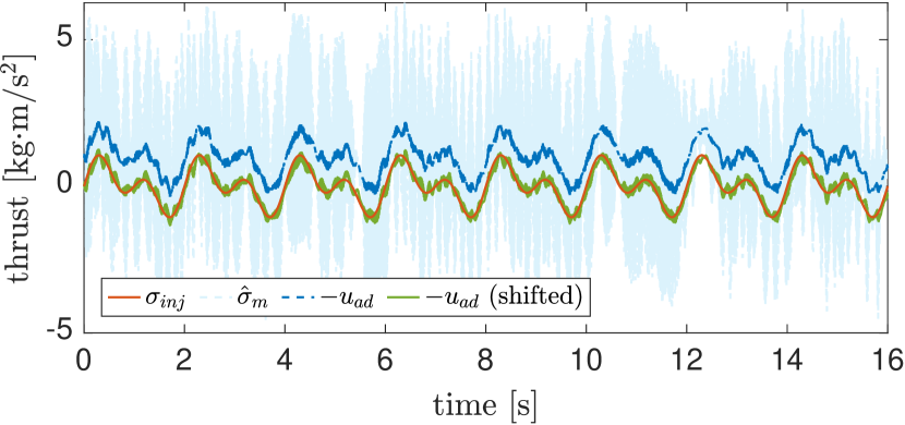
(a) Injected uncertainty $\sigma_{inj}$ with estimation $\hat{\sigma}_{m}$ and compensation $u_{ad}$, all on the thrust channel.

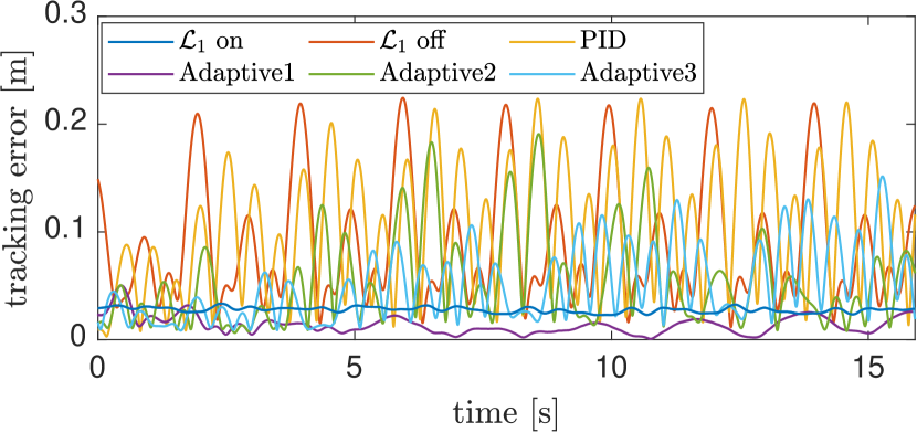
(b) Comparison on the tracking error of the system.

Figure 3: Results for the experiments with injected uncertainties on the thrust channel.

VII-B Slosh payload

Slosh payload is a challenging scenario for the quadrotor’s tracking control: the sloshing liquid constantly changes its distribution within the container, causing constant changes in the vehicle’s center of mass and moment of inertia. Due to the high dimensions of the fluid dynamics, modeling the liquid distribution as a function of the quadrotor’s state is forbidden for real-time computation. In this experiment, we attach a bottle to the bottom of the quadrotor (with the bottle’s longitudinal direction aligned with the quadrotor’s body-$x$ direction) and fill the bottle half-full. The total added weight is 0.317 kg, approximately 50% of the quadrotor’s weight. We command the quadrotor to track a circular trajectory with a 1 m radius and 2.5 m/s linear speed. To track such a trajectory, the quadrotor needs to tilt on the roll or pitch axis for a maximum of 45 degrees, leading to drastic sloshing of the liquid payload, as can be seen in Figure 4(a). The tracking error comparison between the $\mathcal{L}_{1}$ on and off is shown in Figure 4(b). Notably, since the slosh motion majorly happens on the $x$-axis of the quadrotor, there is an apparent improvement in tracking performance on the $x$-axis by the $\mathcal{L}_{1}$ adaptive control. For the total position tracking error, the $\mathcal{L}_{1}$ adaptive control maintains a consistently smaller tracking error than when it is off.

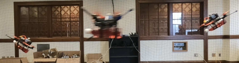
(a) Snapshots of the quadrotor during the slosh payload test. Notice the tilted liquid surface when the quadrotor is at the left and right positions.

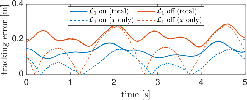
(b) Position tracking error with the slosh payload for $\mathcal{L}_{1}$ on and off. The plots correspond to two rounds of the circular trajectory.

Figure 4: Slosh payload experiment.

VII-C Chipped propeller

In this experiment, we chipped the tip of one propeller (shown in Figure 5(a)). We removed 1/4 of the propeller, which reduces the generated thrust from this propeller.

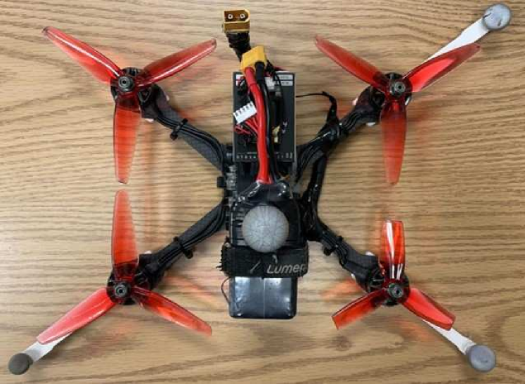
(a)

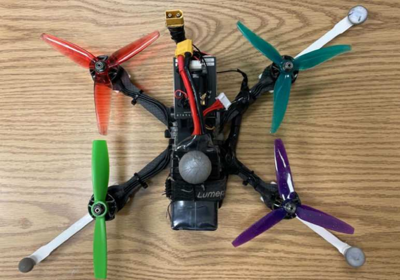
(b)

Figure 5: Quadrotors with (a) a chipped propeller and (b) mixed propellers. The mixed propellers are T-Motor T5150 Tri-Blade Propeller (upper left), HQProp 5$\times$4.5RG Bullnose Propeller (lower left), Gemfan 51466 V2 Tri-Blade Propeller (upper right), and Gemfan 513D Tri-Blade 3D Propeller (bottom right).

The quadrotor takes off to 1 m altitude from $-3.8$ to $-2$ s, during which the $\mathcal{L}_{1}$ adaptive control is turned off. The quadrotor is supposed to hover after $-2$ s. However, due to the thrust loss at the chipped propeller, the quadrotor cannot stabilize itself in the hovering position. This is reflected by the diverging oscillation from $-2$ to $0$ s in Figure 6(a). At 0 s, we turn the $\mathcal{L}_{1}$ adaptive control on. Consequently, the quadrotor can stabilize itself to hover owing to $\mathcal{L}_{1}$’s compensation to the thrust generated by the chipped propeller. We further conduct the test that transitioned the quadrotor from $\mathcal{L}_{1}$ on to $\mathcal{L}_{1}$ off, with results shown in Figure 6(b). The $\mathcal{L}_{1}$ adaptive control is turned off at 0 s, from which moment the quadrotor enters the diverging oscillation, where the wave packet of tracking error grows on all three axes.

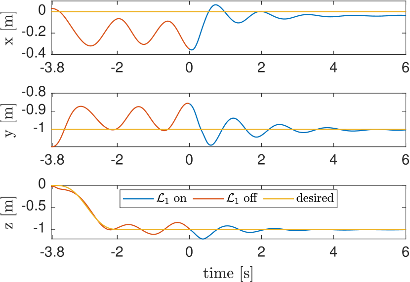
(a) Switching $\mathcal{L}_{1}$ off to $\mathcal{L}_{1}$ on during hover.

(b) Switching $\mathcal{L}_{1}$ on to $\mathcal{L}_{1}$ off during hover.

Figure 6: Transient tracking performance when switching between $\mathcal{L}_{1}$ on and off with one chipped propeller.

We further conduct the experiment to have the quadrotor (with the chipped propeller) follow a circular trajectory with a 1 m radius and 0.5 m/s linear speed. We keep the $\mathcal{L}_{1}$ adaptive control on in this experiment to avoid the divergent oscillation when $\mathcal{L}_{1}$ is off. The actual trajectory is compared to the desired trajectory, as shown in Figure 7(a). The RMSE is 0.045 m. We further show the commanded PWM for each motor in Figure 7(b), where motor 4 (with the chipped propeller) counteracts the thrust loss by commanding a higher PWM than the other motors.

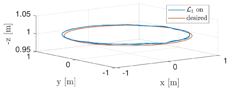
(a) Comparison between the real trajectory and desired trajectory.

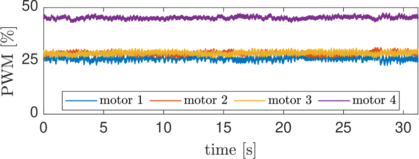
(b) Pulse-width modulation (PWM) for the four motors.

Figure 7: Results for the quadrotor with a chipped propeller circulating at 0.5 m/s with 1 m radius.

VII-D Mixed propellers

In this experiment, we apply four different propellers on the quadrotor (inspired by the experiment in [39]). Figure 5(b) shows the propeller configuration. Since each propeller has its own thrust coefficient, the mixed propellers lead to unbalanced scaling of thrust from each propeller. We command the quadrotor to hover, and the tracking performance is shown in Figure 8. We start with $\mathcal{L}_{1}$ on. When the $\mathcal{L}_{1}$ is turned off at 5 s, the tracking performance deteriorates instantly, and the quadrotor turns into divergent oscillation as time goes on (growing wave packets on all three $x$-, $y$-, and $z$-axis are clear). We switch $\mathcal{L}_{1}$ back on at 26 s, and the $\mathcal{L}_{1}$ adaptive control resumes the stable hover with fast transient and small tracking error just like at the beginning of the experiment.

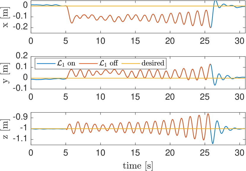
Figure 8: Tracking performance of the quadrotor with mixed propellers.

VII-E Ground effect

The ground effect refers to the aerodynamic effect when the quadrotor flies close to the ground or a surface beneath it. In this experiment, we place a gym mat beneath the quadrotor’s path. The top surface of the mat is at 0.95 m, whereas the desired trajectory’s altitude is 1 m (see Figure 9 for the illustration of the setup). This mat induces the ground effect when the quadrotor flies on top of the mat: we name the area above the mat by “ground effect zone.” The quadrotor’s altitude tracking is majorly impacted due to the reflected downwash when the quadrotor flies through the ground effect zone. Figure 10(a) shows the comparison of altitude tracking between $\mathcal{L}_{1}$ on and off, where the quadrotor enters and leaves the ground effect zone at 1.55 and 4.86 s, respectively. In the case of $\mathcal{L}_{1}$ on, the quadrotor closely tracks the desired altitude despite small perturbations when entering and leaving the ground effect region, with a maximum deviation to be within 1 cm. Since the geometric controller ($\mathcal{L}_{1}$ off) admits a steady-state error, it results in the quadrotor flying at a higher altitude than the case with $\mathcal{L}_{1}$ on. This behavior leads to the quadrotor with $\mathcal{L}_{1}$ off suffering less from the ground effect than the one with $\mathcal{L}_{1}$ on. Despite this fact, the amplitude of perturbation with $\mathcal{L}_{1}$ on is kept smaller than in the case of $\mathcal{L}_{1}$ off.

We show the thrust commands in the cases of $\mathcal{L}_{1}$ on and off in Figure 10(b). It can be seen that the total thrust command (baseline plus $\mathcal{L}_{1}$ adaptive control) is reduced in the ground effect zone when $\mathcal{L}_{1}$ is on, which compensates for the reflected downwash. Additionally, the $\mathcal{L}_{1}$ adaptive control applies a constant offset to compensate for the extra thrust (shown in green in Figure 10(b)) commanded by the geometric controller (which results in the steady-state error if not compensated for). The thrust command in the case of $\mathcal{L}_{1}$ off is also reduced when the quadrotor flies through the ground effect zone. However, the reason for the thrust reduction with $\mathcal{L}_{1}$ off is fundamentally different from the one discussed above when $\mathcal{L}_{1}$ is on. The quadrotor was lifted by the ground effect, which causes a bigger altitude tracking error in the ground effect zone, as shown in Figure 10(a). The lifted altitude leads to reductions in the commanded thrusts as the baseline controller reduces the thrusts to lower the altitude for smaller tracking errors.

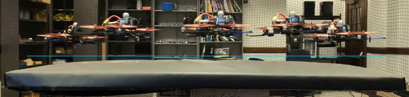
(a) $\mathcal{L}_{1}$ off

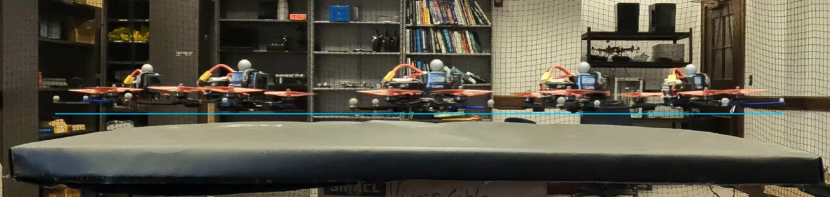
(b) $\mathcal{L}_{1}$ on

Figure 9: The quadrotor flies over the ground effect zone. A blue line is supplied for comparing the altitude tracking performance.

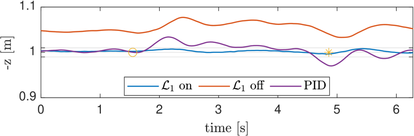
(a) Altitude tracking in the ground effect zone. The desired altitude is 1 m. The circle and star indicate the time of entering and leaving the zone, respectively.

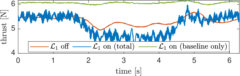
(b) Thrust commands in the ground effect zone for $\mathcal{L}_{1}$ on and off.

Figure 10: Results for the ground effect experiment

VII-F Voltage drop

In this experiment, we test the influence of the battery’s voltage drop on the tracking performance. Voltage drop is a common issue for quadrotors, as the ubiquitously used Lithium polymer (LiPo) battery’s voltage drops from 4.2 V (fully charged) to 3.2 V (minimum voltage for healthy battery) for each cell when discharged. The varying voltage during the quadrotor’s flight will affect the generated thrust on each rotor if not compensated. Specifically, the thrust reduces quadratically to the drop in battery voltage when the duty cycle command remains the same. We command the quadrotor to hover at 1 m while carrying a 0.5 kg payload. The extra payload is used to expedite the battery discharging process. For the altitude tracking, as shown in Figure 11(a), the altitude with $\mathcal{L}_{1}$ on stays steady on 1 m, whereas the altitude with $\mathcal{L}_{1}$ off drops as the voltage drops. It is worth noting that an initial altitude tracking error exists, which is caused by the extra payload and steady-state error of a geometric controller ($\mathcal{L}_{1}$ off). Figure 11(b) shows the voltage drop with $\mathcal{L}_{1}$ on and off. The voltage drop is almost identical in these two cases.

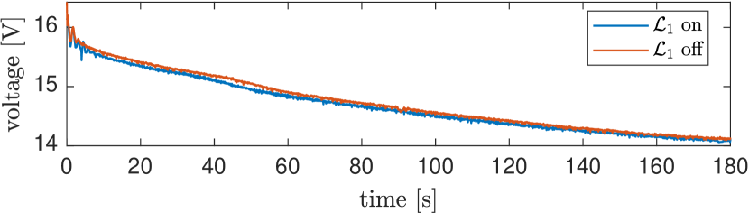
(a) Battery voltage during hover.

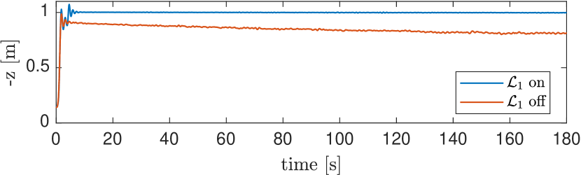
(b) Altitude of the quadrotor.

Figure 11: Results for the compensation of battery voltage drop by the $\mathcal{L}_{1}$ adaptive control.

VII-G Downwash

In this experiment, we test the trajectory tracking performance subject to downwash. Downwash is the complex disturbance generated by one rotorcraft on top of another vehicle, which severely degrades the attitude and position tracking of the latter. It is generally difficult to establish an accurate model based on the relative motion between two vehicles. Hence, adaptive control methods are preferred. We command a heavier quadrotor (1.4 kg) to hover at 1.6 m altitude, right on top of one point on the trajectory of the tested quadrotor. The comparison on the altitude tracking performance between $\mathcal{L}_{1}$ on, $\mathcal{L}_{1}$ off, and PID are shown in Figure 13, with the downwash starting to affect the tested quadrotor around 1.5 s. The altitude tracking displayed in Figure 13 indicates that the $\mathcal{L}_{1}$ adaptive control can quickly capture the effect of downwash and compensate for it, resulting in fast transient response, whereas the quadrotor without compensation ($\mathcal{L}_{1}$ off) experienced instant deviation from the desired altitude by around 0.3 m. The PID controller performs poorly with a similar amount of deviation as in the case with $\mathcal{L}_{1}$ off. The analysis of the poor performance of the PID controller is similar to the injected uncertainty case in Section VII-A: the fast-changing downwash leads to insufficient integration on the integral term to counteract the downwash timely.

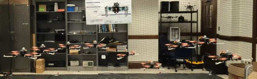
(a) $\mathcal{L}_{1}$ off

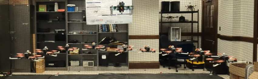
(b) $\mathcal{L}_{1}$ on

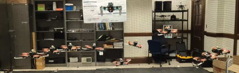
(c) PID

Figure 12: Snapshots of the downwash experiment. The snapshots are taken from 0 s to 3.14 s corresponding to Figure 13 with equal time intervals.

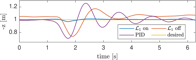
Figure 13: Altitude tracking in the experiments with downwash. The downwash starts to influence the quadrotor around 1.5 s. The heavier quadrotor that generates the downwash drifted around the desired hover position by 0.1 m, which leads to the different start time of downwash of the tested quadrotor.

VII-H Tunnel

In this experiment, we command the quadrotor to fly through a tunnel with 0.6 m (H) $\times$ 0.6 m (W) $\times$ 1.2 m (D). The tunnel is built to mimic the flying condition in confined space, e.g., a cave or mine passageway, where the quadrotor itself induces and therefore experiences complex airflow. We use Acrylic sheets for their transparency, which permits Vicon localization inside the tunnel. As shown in Figure 14(a). the quadrotor flies from left to right following the trajectory $-1.2\cos(1/1.2t)$ with altitude of 0.3 m. Comparison of the tracking errors of $\mathcal{L}_{1}$ on, $\mathcal{L}_{1}$ off, and PID is shown in Figure 14(b). With $\mathcal{L}_{1}$ on, the quadrotor achieves the minimum tracking error (within 0.03 m) while staying consistently smaller than with $\mathcal{L}_{1}$ off or PID. The latter two cases have the maximum tracking error that triples the one with $\mathcal{L}_{1}$ on, favoring $\mathcal{L}_{1}$ adaptive control in the environment with confined space.

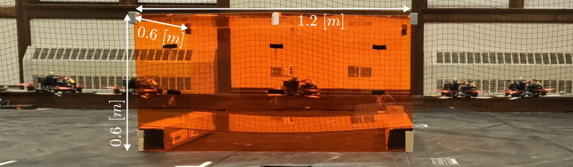
(a) Snapshot of the tunnel experiment with $\mathcal{L}_{1}$ on.

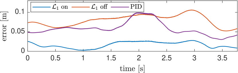
(b) Tracking error of the compared controllers. The quadrotor enters and leaves the tunnel at around 1.26 s and 2.51 s, respectively.

Figure 14: Results for the tunnel experiment.

VII-I Hanging off-center weights

In this experiment, we hang weights to the quadrotor amid hovering. Specifically, the weights are hung right beneath the front-left motor, which is off the quadrotor’s center of gravity. This experiment is a simplified scenario of delivery drones that picks up a package, albeit at an off-center location. We exaggerate the case by extending the off-center location to be under one motor. The weights will introduce force and moment to the quadrotor in this setting, adding the complexity of stabilizing the quadrotor. We hang weights of 100, 200, and 300 g in the experiments. The tracking errors in these three cases are shown in Figure 15. We compare three controller cases: $\mathcal{L}_{1}$ off, $\mathcal{L}_{1}$ on, and PID. As the weight increases, the tracking error increases for all cases. $\mathcal{L}_{1}$ off shows the worst tracking performance and eventually crashes the quadrotor once the 300 g weight is hung. $\mathcal{L}_{1}$ on and PID demonstrate similar performance, with $\mathcal{L}_{1}$ on having a slight advantage in fast transient and smaller steady-state error.

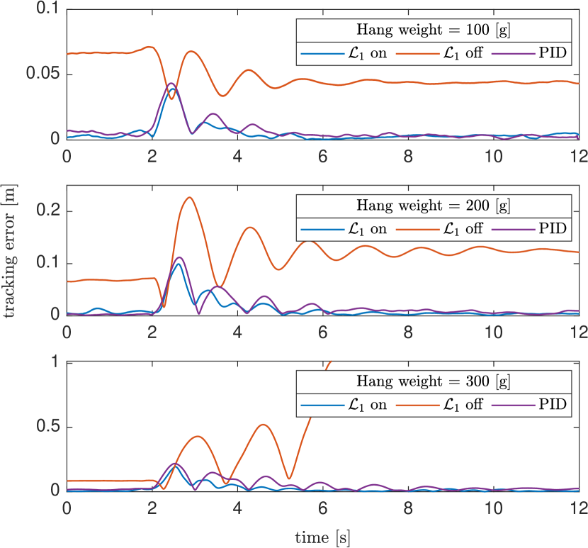
Figure 15: Tracking error of the quadrotor when hanging off-center weights in it starting at 2 s.

VII-J Benchmark experiments with added weights and slung weights

We would like to know the systematic performance improvement by the $\mathcal{L}_{1}$ adaptive control in addition to the case-by-case scenarios in the experimental results shown above. For the systematic experiment, we attach weights to the bottom of the quadrotor, where the weights range from 100 to 500 g with 100 g increments. We refer to this case as “added weights.” We also include the “slung weights,” where the weights are hung by a cord with 0.4 m length. For both types of weights, we command the quadrotor to fly two trajectories: 1) a 1 m radius circular trajectory with linear speed ranging from 0 (hover) to 2.5 m/s with a 0.5 m/s increment and 2) a figure 8 trajectory with the maximum speed ranging from 0 (hover) to 3 m/s with a 1 m/s increment. The comparisons on the tracking error among $\mathcal{L}_{1}$ off, $\mathcal{L}_{1}$ on, and PID are shown in Figure 16 (circular trajectory) and Figure 17 (figure 8 trajectory). For each case, data within 5 s (4000 data points in total) are used to make the box plots.

On the one hand, the tracking errors with $\mathcal{L}_{1}$ on are significantly smaller than with $\mathcal{L}_{1}$ off with the same trajectory, speed, and type of weights. On the other hand, with the same trajectory and speed, the tracking error with $\mathcal{L}_{1}$ on stays consistent despite the gradually increased weights. This consistency does not show up when $\mathcal{L}_{1}$ is off, since the tracking errors grow as the weights increase. PID performs considerably better than $\mathcal{L}_{1}$ off, with similar (and sometimes smaller) errors to that of $\mathcal{L}_{1}$ off. However, in extreme cases with relatively large weights and high speeds, PID cannot stabilize the quadrotor and eventually crashes the vehicle, as indicated by the red crosses in Figure 17(b). This happens, again, due to the incapability of PID in handling fast-changing uncertainties: in this case, the uncertainties come from the swing of the slung weights during the figure-8 maneuver. The RMSE comparisons are shown in Tables II and III for the circle trajectory and Tables IV and V for the figure 8 trajectory in Appendix -E.

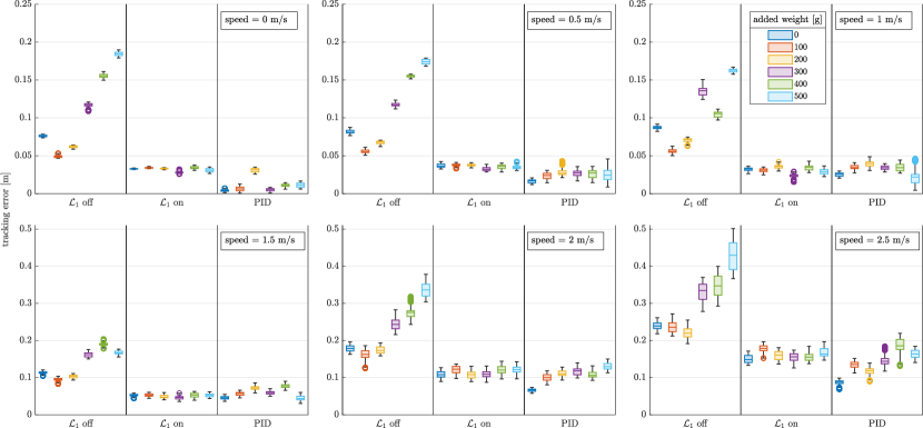
(a) Added weights

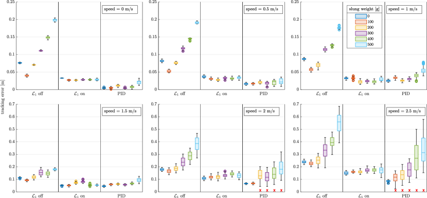
(b) Slung weights

Figure 16: Tracking errors of the quadrotor when following a circular trajectory. The red crosses indicate that the trials crashed.

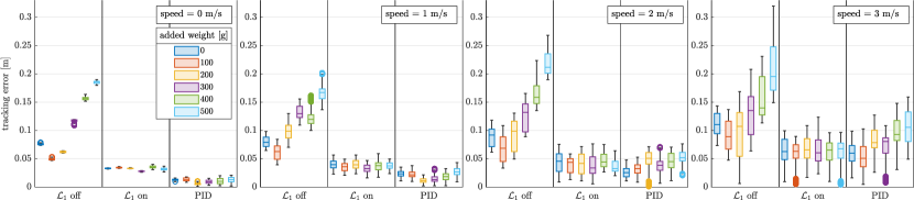
(a) Added weights

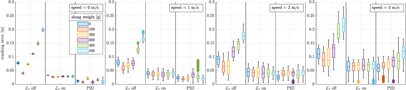
(b) Slung weights

Figure 17: Tracking errors of the quadrotor when following a figure 8 trajectory.

VIII Conclusion

In this paper, we present $\mathcal{L}_{1}$Quad, an $\mathcal{L}_{1}$ adaptive control design for quadrotors. Our design augments a geometric controller with an $\mathcal{L}_{1}$ adaptive controller for both rotational and translational dynamics. We lump the uncertainties as unknown forces and moments, which can be quickly estimated and compensated for by the $\mathcal{L}_{1}$ adaptive control. No case-by-case modeling of the uncertainties is required, which makes the architecture applicable to uncertainties in a wide spectrum of applications.

Theoretically, we prove that the piecewise-constant adaptation law can estimate uncertainties with the error proportional to the sampling time, which can be made arbitrarily small subject only to hardware limitations. With the fast and accurate uncertainty estimation, $\mathcal{L}_{1}$Quad enables computable uniform and uniform ultimate bounds, which guarantees the tracking performance of the quadrotor. Furthermore, the width of the ultimate bound can be adjusted by tuning the filter bandwidth of the low-pass filter and the sampling time.

Experimentally, we validate our approach on a custom-built quadrotor through extensive experiments with various types of uncertainties. The superior performance of $\mathcal{L}_{1}$Quad is illustrated by its consistently smaller tracking error when compared with other controllers in all the experiments, where only one set of controller parameters is used in $\mathcal{L}_{1}$Quad.

Future work includes incorporating the current bounds in the safe feedback motion planning architecture [44] and applying learning techniques (e.g., [45]) to better characterize the uncertainties using data. Learned information could be incorporated into the proposed control framework, which alleviates the workload for $\mathcal{L}_{1}$ adaptive controller and achieves better performance without sacrificing the robustness of the system.

-A Proof of Proposition 1

The original proof in [41, Appendix D, Section (c)] restricts the stability analysis to a compact domain. We rewrite the proof in [41, Appendix D Part (c) and Part (d)] (starting from [41, (79)]) and avoid this restriction.

Proof:

Consider the following Lyapunov function candidate for the translation dynamics:

$$V_{1}=\frac{1}{2}K_{p}\left\|e_{p}\right\|^{2}+\frac{1}{2}m\left\|e_{v}\right\|^{2}+c_{1}e_{p}\cdot e_{v}$$ (41)

with $c_{1}$ being a positive constant. The time derivative of $V_{1}$ is

$$\dot{V}_{1}= K_{p}e_{p}\cdot e_{v}+e_{v}\cdot\left(-K_{p}e_{p}-K_{v}e_{v}-X\right)+c_{1}e_{v}\cdot e_{v}$$

$$+\frac{c_{1}}{m}e_{p}\cdot\left(-K_{p}e_{p}-K_{v}e_{v}-X\right),$$

where we applied the equality $m\dot{e}_{v}=-K_{p}e_{p}-K_{v}e_{v}-X$ with

$$X=\frac{f}{e_{3}^{\top}R_{d}^{\top}Re_{3}}\left((e_{3}^{\top}R_{d}^{\top}Re_{3})Re_{3}-R_{d}e_{3}\right).$$

Rearranging the equation above, we obtain

$$\dot{V}_{1}= -(K_{v}-c_{1})\left\|e_{v}\right\|^{2}-\frac{c_{1}K_{p}}{m}\left\|e_{p}\right\|^{2}$$

$$-\frac{c_{1}K_{v}}{m}e_{p}\cdot e_{v}+X\cdot\left(-\frac{c_{1}}{m}e_{p}-e_{v}\right).$$

Since $X$ is bounded $\left\|X\right\|\leq\left(K_{p}\left\|e_{p}\right\|+K_{v}\left\|e_{v}\right\|+H\right)\left\|e_{R}\right\|$ [41, (81)], and $H>\left\|-mg+m\ddot{x}_{d}\right\|$ [41, (25)], using Cauchy-Schwarz inequality, we have

$$\dot{V}_{1}\leq -(K_{v}-c_{1})\left\|e_{v}\right\|^{2}-\frac{c_{1}K_{p}}{m}\left\|e_{p}\right\|^{2}-\frac{c_{1}K_{v}}{m}e_{p}\cdot e_{v}$$

$$+\left(K_{p}\left\|e_{p}\right\|+K_{v}\left\|e_{v}\right\|+H\right)\left\|e_{R}\right\|\left(\frac{c_{1}}{m}\left\|e_{p}\right\|+\left\|e_{v}\right\|\right).$$ (42)

Our proof will deviate from the original proof now. Define $\alpha>0$ such that $\left\|e_{R}\right\|\leq\alpha<1$ [41, Before (81)]. Plugging $\alpha$ in the inequality above, we have

$$\dot{V}_{1}\leq -(K_{v}(-\alpha+1)-c_{1})\left\|e_{v}\right\|^{2}-\frac{c_{1}K_{p}}{m}(1-\alpha)\left\|e_{p}\right\|^{2}$$

$$+\left(\frac{c_{1}K_{v}}{m}(1+\alpha)+K_{p}\alpha\right)\left\|e_{p}\right\|\left\|e_{v}\right\|$$

$$+\left\|e_{R}\right\|\left(\frac{c_{1}}{m}H\left\|e_{p}\right\|+H\left\|e_{v}\right\|\right).$$ (43)

We define the Lyapunov candidate $V_{2}$ for the rotational dynamics in the same way as in [41, (57)]:

$$V_{2}=\frac{1}{2}e_{\Omega}\cdot Je_{\Omega}+K_{R}\Psi(R,R_{d})+c_{2}e_{R}\cdot e_{\Omega},$$

with a positive constant $c_{2}$. The Lyapunov candidate for the complete dynamics is $V=V_{1}+V_{2}$ where $V$ is defined in (1). Using the bound $\frac{1}{2}\left\|e_{R}\right\|^{2}\leq\Psi(R,R_{d})\leq\frac{1}{2-\psi_{1}}\left\|e_{R}\right\|^{2}$ in [41, Equ 73], the Lyapunov candidate is bounded by

$$z_{1}^{\top}M_{11}z_{1}+z_{2}^{\top}M_{21}z_{2}\leq V\leq z_{1}^{\top}M_{12}z_{1}+z_{2}^{\top}M_{22}z_{2},$$ (44)

where $z_{1}=[\left\|e_{p}\right\|,\left\|e_{v}\right\|]^{\top}$, $z_{2}=[\left\|e_{R}\right\|,\left\|e_{\Omega}\right\|]^{\top}$, and the matrices $M_{11}$, $M_{12}$, $M_{21}$, and $M_{22}$ are defined in Section VI. Furthermore,

$$\lambda_{m}(M_{11})\left\|z_{1}\right\|^{2}+\lambda_{m}(M_{21})\left\|z_{2}\right\|^{2}\leq V\\ \leq\lambda_{M}(M_{12})\left\|z_{1}\right\|^{2}+\lambda_{M}(M_{22})\left\|z_{2}\right\|^{2}.$$ (45)

Next, we derive the bound on $\dot{V}=\dot{V}_{1}+\dot{V}_{2}$. The bound on $\dot{V}_{1}$ is shown in (-A). For $\dot{V}_{2}$, we follow the derivation in [41, (58)]

$$\dot{V}_{2}= -K_{\Omega}\left\|e_{\Omega}\right\|^{2}-c_{2}K_{R}e_{R}\cdot J^{-1}e_{R}+c_{2}C(R_{d}^{\top}R)e_{\Omega}\cdot e_{\Omega}$$

$$-c_{2}K_{\Omega}e_{R}\cdot J^{-1}e_{\Omega},$$ (46)

where $C(R_{d}^{\top}R)=\left(\text{tr}(R^{\top}R_{d})I-R^{\top}R_{d}\right)/2$, and $\left\|C(R_{d}^{\top}R)\right\|_{2}\leq 1$ [41, (54)]. The derivative $\dot{V}$ is bounded by

$$\dot{V}\leq-z_{1}^{\top}W_{1}z_{1}+z_{1}^{\top}W_{12}z_{2}-z_{2}^{\top}W_{2}z_{2},$$ (47)

where $W_{1}$, $W_{12}$, $W_{2}$ are defined in Section VI. We choose positive constants $K_{p}$, $K_{v}$, $K_{\Omega}$, $K_{R}$, $c_{1}$, and $c_{2}$ such that $M_{11}$, $M_{21}$, $M_{12}$, $M_{22}$, $W_{1}$, and $W_{2}$ are positive definite matrices, and $W\succ 0$ where $W$ is defined in (14). Therefore, $\dot{V}$ is negative-definite, and the zero equilibrium of the closed-loop tracking errors $(\left\|e_{p}\right\|,\left\|e_{v}\right\|,\left\|e_{R}\right\|,\left\|e_{\omega}\right\|)$ is exponentially stable. Specifically, we have

$$\dot{V}\leq-\beta V,$$ (48)

where $\beta$ is defined in (19). Also, using Definition 2 and (44), we have

$$\underline{\gamma}d(x,x_{d})^{2}\leq V\leq\overline{\gamma}d(x,x_{d})^{2},$$ (49)

where $\underline{\gamma}$ and $\overline{\gamma}$ are defined in (20) and (21), respectively. Without loss of generality, we consider $K_{p}$, $K_{v}$, $K_{R}$, $K_{\Omega}$ to be scalars for simplicity. However, the extension to the diagonal 3-by-3 matrices is straightforward, where maximum or minimum eigenvalues of these matrices will be used in the derived bounds when appropriate. ∎

-B Proof of Proposition 3

Proof:

Since $x(t)\in\mathcal{O}(x_{d}(t),\rho)$, we have $\left\|e_{p}\right\|$, $\left\|e_{v}\right\|,$ $\left\|e_{\Omega}\right\|$, and $\left\|e_{R}\right\|$ upper bounded by $\rho$ (following the definition of $\mathcal{O}(x_{d}(t),\rho)$ in Definition 2). Considering that $c_{1}$ and $m$ are constants and $\left\|Re_{3}\right\|=1$ by the definition of the rotation matrix, we can conclude that all three bounds in (26) hold. Furthermore, following the control law in (2) and (III), we conclude $\left\|u_{b}\right\|$ is also bounded. Define $\Delta_{u_{b}}$ such that $\left\|u_{b}\right\|\leq\Delta_{u_{b}}$.

In order to prove that $\left\|u_{ad}\right\|$ is bounded, we need to show $\left\|\hat{\sigma}(iT_{s})\right\|$ is bounded for all $i\in\mathbb{N}$. We use proof by induction. When $t=0$, $\left\|\hat{\sigma}(0)\right\|=0$. Assume that $\left\|\hat{\sigma}(iT_{s})\right\|$ is bounded for an arbitrary $i\geq 1$. Since $A_{s}$ is a Hurwitz matrix, the prediction error dynamics in (10) is bounded-input, bounded-output stable. Using the bounds on $\sigma(t)$ and $\bar{B}(t)$ for $t\in[iT_{s},(i+1)T_{s})$ in Assumption 1 and (24), respectively, we conclude $\tilde{z}((i+1)T_{s})$ is bounded. Consider the adaptation law in (9) and the bound on $\bar{B}^{-1}(iT_{s})$ in (24); then we conclude $\hat{\sigma}((i+1)T_{s})$ is bounded. Thus, $\left\|\hat{\sigma}(iT_{s})\right\|$ is bounded for all $i\in\mathbb{N}$. Define $\Delta_{\hat{\sigma}}$ such that

$$\left\|\hat{\sigma}(iT_{s})\right\|\leq\Delta_{\hat{\sigma}}$$ (50)

for all $i\in\mathbb{N}$. Since $C(s)=\omega/\left(s+\omega\right)$ with DC gain equal to 1, we have $\left\|C(s)\right\|_{\mathcal{L}_{1}}=1$. Following [20, Lemma A.7.1], we obtain $\left\|u_{ad}(t)\right\|\leq\left\|C(s)\right\|_{\mathcal{L}_{1}}\left\|\hat{\sigma}(t)\right\|_{\mathcal{L}_{\infty}}\leq\Delta_{\hat{\sigma}}$. ∎

-C Proof of Proposition 4

Before proving Proposition 4, we first introduce the following proposition.

Proposition 5

If the state $x(t)$ of the uncertain system in (V) satisfies $x(t)\in\mathcal{O}(x_{d}(t),\rho)$ for all $t\in[0,\tau]$ with some $\tau>0$, then the following inequality holds

$$\left\|\dot{x}\right\|_{\mathcal{L}_{\infty}}^{[0,\tau]}\leq\Delta_{f}+\Delta_{\bar{B}}\Delta_{\sigma}+\Delta_{B_{F}}(\Delta_{u_{b}}+\Delta_{\hat{\sigma}}).$$ (51)

Proof:

Using the dynamics of the uncertain system in (V), we obtain

$$\left\|\dot{x}(t)\right\|\leq \left\|f(x(t))\right\|+\left\|\bar{B}_{F}(R(t))\right\|\left\|\sigma(t,x(t))\right\|$$

$$+\left\|B_{F}(R(t))\right\|\left\|u_{b}(t)+u_{ad}(t)\right\|.$$ (52)

With the help of the bounds in Assumption 1, (24), (26), and (27), we can conclude that

$$\left\|\dot{x}\right\|_{\mathcal{L}_{\infty}}^{[0,\tau]}\leq\Delta_{f}+\Delta_{\bar{B}}\Delta_{\sigma}+\Delta_{B_{F}}(\Delta_{u_{b}}+\Delta_{\hat{\sigma}})=\phi_{1},$$

where $\phi_{1}$ is defined in (28). ∎

We now move to prove Proposition 4.

Proof:

We first derive the bound on $\left\|\hat{\sigma}(t,x(t))-\sigma(t,x(t))\right\|$ for any $t\in[(i+1)T_{s},(i+2)T_{s})$, where $i\in\mathbb{N}$. The bound on $\left\|\hat{\sigma}(t,x(t))-\sigma(t,x(t))\right\|$ for $t\in[0,T_{s})$ will be discussed at the end of this section. Substituting the adaptation law (9) for $\hat{\sigma}(iT_{s})$ in (V), we can compute the prediction error:

$$\tilde{z}((i+1)T_{s})=-\textstyle\int_{iT_{s}}^{(i+1)T_{s}}\exp(A_{s}((i+1)T_{s}-\tau))\\ \bar{B}(\tau)\sigma(\tau)\text{d}\tau+\Phi_{0}((i+1)T_{s}),$$ (53)

where

$$\Phi_{0}((i+1)T_{s})\triangleq\textstyle\int_{iT_{s}}^{(i+1)T_{s}}\exp(A_{s}((i+1)T_{s}-\tau))\\ (\bar{B}(\tau)-\bar{B}(iT_{s}))\hat{\sigma}(iT_{s})\text{d}\tau.$$ (54)

Since $z(t)$ and $\bar{B}(t)$ are continuous and $\sigma(t)$ is continuous by Assumption 1, considering that every diagonal element in $\exp(A_{s}((i+1)T_{s}-\tau))$ is positive, we apply the mean value theorem in an element-wise manner to the first integral on the right-hand side of (53), which leads to

$$-\textstyle\int_{iT_{s}}^{(i+1)T_{s}}\exp(A_{s}((i+1)T_{s}-\tau))\bar{B}(\tau)\sigma(\tau)\text{d}\tau$$

$$= -\textstyle\int_{iT_{s}}^{(i+1)T_{s}}\exp(A_{s}((i+1)T_{s}-\tau))\text{d}\tau\bar{B}^{\ast}\sigma^{\ast}$$

$$= A_{s}^{-1}(I-\exp(A_{s}T_{s}))\bar{B}^{\ast}\sigma^{\ast},$$ (55)

where

$$(\bar{B}^{\ast}\sigma^{\ast})_{i}\triangleq(\bar{B}(\tau_{i})\sigma(\tau_{i}))_{i}$$

for $i=1,\dots,6$ and $\tau_{1},\dots,\tau_{6}\in[iT_{s},(i+1)T_{s})$. Applying the mean value theorem in an element-wise manner to $\Phi_{0}$, we obtain

$$\Phi_{0}((i+1)T_{s})=-A_{s}^{-1}(I-\exp(A_{s}T_{s}))\bar{B}^{\#}\hat{\sigma}^{\#},$$ (56)

where

$$(\bar{B}^{\#}\hat{\sigma}^{\#})_{i}\triangleq\left((\bar{B}(\beta_{i})-\bar{B}(iT_{s}))\hat{\sigma}(iT_{s})\right)_{i}$$

for $i=1,\dots,6$ and $\beta_{1},\dots,\beta_{6}\in[iT_{s},(i+1)T_{s})$. Plugging (56) and (-C) in (53), we have

$$\tilde{z}((i+1)T_{s})=A_{s}^{-1}(I-\exp(A_{s}T_{s}))\left(\bar{B}^{\ast}\sigma^{\ast}-\bar{B}^{\#}\hat{\sigma}^{\#}\right).$$ (57)

To compute the uncertainty estimates, plug in the prediction error in (57) to (9) for $t\in[(i+1)T_{s},(i+2)T_{s})$; then we have

$$\hat{\sigma}\left((i+1)T_{s}\right)= \bar{B}((i+1)T_{s})^{-1}\exp(A_{s}T_{s})\left(\bar{B}^{\ast}\sigma^{\ast}\right.$$

$$-\left.\bar{B}^{\#}\hat{\sigma}^{\#}\right).$$ (58)

The results from Proposition 5 imply that for $\tau_{j}\in[iT_{s},(i+1)T_{s})$ and $t\in[(i+1)T_{s},(i+2)T_{s})$

$$\left\|x(t)-x(\tau_{j})\right\|\leq\textstyle\int_{\tau^{\ast}}^{t}\left\|\dot{x}(\tau)\right\|\text{d}\tau\leq 2T_{s}\phi_{1}.$$

Now we are ready to compute $\left\|\sigma(t)-\hat{\sigma}(t)\right\|$ for $t\in[(i+1)T_{s},(i+2)T_{s})$, which is shown in (59).

Using (-C), we have

$$\left\|\sigma(t)-\hat{\sigma}(t)\right\|= \left\|\sigma(t)-\bar{B}((i+1)T_{s})^{-1}\exp(A_{s}T_{s})\left(\bar{B}^{\ast}\sigma^{\ast}-\bar{B}^{\#}\hat{\sigma}^{\#}\right)\right\|$$

$$\leq \left\|\bar{B}((i+1)T_{s})^{-1}(\bar{B}((i+1)T_{s}))\sigma(t)-\exp(A_{s}T_{s})\bar{B}^{\ast}\sigma^{\ast})\right\|+\left\|\bar{B}((i+1)T_{s})^{-1}\exp(A_{s}T_{s})\bar{B}^{\#}\hat{\sigma}^{\#}\right\|$$

$$\leq \sqrt{6}\left\|\bar{B}((i+1)T_{s})^{-1}\right\|\left\|\bar{B}((i+1)T_{s}))\sigma(t)-\exp(A_{s}T_{s})\bar{B}^{\ast}\sigma^{\ast}\right\|_{\infty}+\sqrt{6}\left\|\bar{B}((i+1)T_{s})^{-1}\right\|\left\|\exp(A_{s}T_{s})\bar{B}^{\#}\hat{\sigma}^{\#}\right\|_{\infty}$$

$$= \sqrt{6}\left\|\bar{B}((i+1)T_{s})^{-1}\right\|\left|(\bar{B}((i+1)T_{s}))\sigma(t)-\exp(A_{s}T_{s})\bar{B}^{\ast}\sigma^{\ast})_{j}\right|+\sqrt{6}\left\|\bar{B}((i+1)T_{s})^{-1}\right\|\left|(\exp(A_{s}T_{s})\bar{B}^{\#}\hat{\sigma}^{\#})_{k}\right|$$

$$\leq \sqrt{6}\left\|\bar{B}((i+1)T_{s})^{-1}\right\|\left\|\bar{B}((i+1)T_{s}))\sigma(t)-\exp(A_{s}T_{s})\bar{B}(\tau_{j})\sigma(\tau_{j})\right\|$$

$$+\sqrt{6}\left\|\bar{B}((i+1)T_{s})^{-1}\right\|\left\|\exp(A_{s}T_{s})\left(\bar{B}(\beta_{k})-\bar{B}(iT_{s})\right)\hat{\sigma}(iT_{s})\right\|,$$ (59)

where $j\triangleq\arg\max_{j\in\{1,\dots,6\}}\left|(\bar{B}((i+1)T_{s}))\sigma(t)-\exp(A_{s}T_{s})\bar{B}^{\ast}\sigma^{\ast})_{j}\right|$, and $k\triangleq\arg\max_{k\in\{1,\dots,6\}}\left|(\exp(A_{s}T_{s})\bar{B}^{\#}\hat{\sigma}^{\#})_{k}\right|$.

Following equation (59), we have

$$\left\|\sigma(t)-\hat{\sigma}(t)\right\|\leq \sqrt{6}\left\|\bar{B}((i+1)T_{s})^{-1}\right\|\left\|\bar{B}((i+1)T_{s}))\sigma(t)-\exp(A_{s}T_{s})\bar{B}(\tau_{j})\sigma(\tau_{j})\right\|$$

$$+\sqrt{6}\left\|\bar{B}((i+1)T_{s})^{-1}\right\|\left\|\exp(A_{s}T_{s})\left(\bar{B}(\beta_{k})-\bar{B}(iT_{s})\right)\hat{\sigma}(iT_{s})\right\|$$

$$\leq \sqrt{6}\left\|\bar{B}((i+1)T_{s})^{-1}\right\|\left(\left\|\bar{B}((i+1)T_{s})\right\|\left\|\sigma(t)-\sigma(\tau_{j})\right\|+\left\|\bar{B}((i+1)T_{s})\sigma(\tau_{j})-\exp(A_{s}T_{s})\bar{B}(\tau_{j})\sigma(\tau_{j})\right\|\right)$$

$$+\sqrt{6}\left\|\bar{B}((i+1)T_{s})^{-1}\right\|\left\|\exp(A_{s}T_{s})\left(\bar{B}(\beta_{k})-\bar{B}(iT_{s})\right)\hat{\sigma}(iT_{s})\right\|$$

$$\leq \sqrt{6}\left\|\bar{B}((i+1)T_{s})^{-1}\right\|\left(\left\|\bar{B}((i+1)T_{s})\right\|\left\|\sigma(t)-\sigma(\tau_{j})\right\|+\left\|\exp(A_{s}T_{s})\left(\bar{B}(\beta_{k})-\bar{B}(iT_{s})\right)\hat{\sigma}(iT_{s})\right\|\right)$$

$$+\sqrt{6}\left\|\bar{B}((i+1)T_{s})^{-1}\right\|\left(\left\|\bar{B}((i+1)T_{s})-\bar{B}(\tau_{j})\right\|+\left\|(I-\exp(A_{s}T_{s})\bar{B}(\tau_{j}))\right\|\right)\left\|\sigma(\tau_{j})\right\|$$

$$= \Phi_{1}(t)+\Phi_{2}(t)+\Phi_{3}(t),$$ (60)

where

$$\Phi_{1}(t)\triangleq \sqrt{6}\left\|\bar{B}((i+1)T_{s})^{-1}\right\|\left\|\bar{B}((i+1)T_{s})\right\|\left\|\sigma(t)-\sigma(\tau_{j})\right\|,$$

$$\Phi_{2}(t)\triangleq \sqrt{6}\left\|\bar{B}((i+1)T_{s})^{-1}\right\|\left\|\bar{B}((i+1)T_{s})-\bar{B}(\tau_{j})\right\|\left\|\sigma(\tau_{j})\right\|+\sqrt{6}\left\|\bar{B}((i+1)T_{s})^{-1}\right\|\left\|(I-\exp(A_{s}T_{s}))\bar{B}(\tau_{j})\right\|\left\|\sigma(\tau_{j})\right\|,$$

$$\Phi_{3}(t)\triangleq \sqrt{6}\left\|\bar{B}((i+1)T_{s})^{-1}\right\|\left\|\exp(A_{s}T_{s})\left(\bar{B}(\beta_{k})-\bar{B}(iT_{s})\right)\hat{\sigma}(iT_{s})\right\|,$$

with $\tau_{j}$ and $\beta_{k}\in[iT_{s},(i+1)T_{s})$.

To compute the estimation error bound, we compute the bound on $\Phi_{1}$, $\Phi_{2}$, and $\Phi_{3}$ in (-C) separately. We first derive the bound on $\Phi_{1}$. Since $\sigma(t,x(t))$ is Lipschitz due to Assumption 1, using the bounds of $\left\|\bar{B}\right\|$ and $\left\|\bar{B}^{-1}\right\|$ in (24), we have

$$\left\|\Phi_{1}\right\|\leq 2\sqrt{6}T_{s}\Delta_{\bar{B}}\Delta_{\bar{B}^{-1}}\left(\phi_{1}L_{\sigma_{x}}+L_{\sigma_{t}}\right),$$ (61)

where $L_{\sigma_{x}}$ and $L_{\sigma_{t}}$ are the Lipschitz constants of $\sigma(t,x(t))$ with respect to the state $x$ and time $t$, respectively. Next, we derive the bound on $\Phi_{2}$. Notice that $\bar{B}(t)=\bar{B}(R(t))=\left[B(R(t))\ B^{\bot}(R(t))\right]=\left[\begin{smallmatrix}-m^{-1}R(t)e_{3}&0_{3\times 3}&m^{-1}R(t)e_{1}&m^{-1}R(t)e_{2}\\ 0_{3\times 1}&J^{-1}&0_{3\times 1}&0_{3\times 1}\end{smallmatrix}\right]$, since we assumed $x(t)\in\mathcal{O}(x_{d}(t),\rho)$, $\left\|\Omega\right\|$ is bounded. Thus, $\dot{R}$ is bounded because $\dot{R}=R\Omega^{\wedge}$ from (1c). We then conclude that $\left\|\dot{\bar{B}}(t)\right\|$ is bounded and define $L_{B}$ such that $\left\|\dot{\bar{B}}(t)\right\|\leq L_{B}$. With the help of $L_{B}$, we have

$$\left\|\bar{B}((i+1)T_{s})-\bar{B}(\tau_{j})\right\|\leq 2L_{B}T_{s}.$$ (62)

Using the inequality in (62) and the bound of $\left\|\bar{B}^{-1}\right\|$, $\left\|\bar{B}\right\|$ in (24), we have

$$\left\|\Phi_{2}\right\|\leq \sqrt{6}\Delta_{\bar{B}^{-1}}\left(2L_{B}T_{s}+\left\|I-\exp(A_{s}T_{s})\right\|\Delta_{\bar{B}}\right)\Delta_{\sigma}$$ (63)

$$\leq \sqrt{6}\Delta_{\bar{B}^{-1}}T_{s}\left(2L_{B}+\left|\lambda_{m}(A_{s})\right|\Delta_{\bar{B}}\right)\Delta_{\sigma}.$$

Finally, using (62), the bound of $\left\|\bar{B}^{-1}\right\|$ in (24), and the bound of $\hat{\sigma}$ in (50), we have

$$\left\|\Phi_{3}\right\|\leq 2\sqrt{6}\Delta_{\bar{B}^{-1}}\Delta_{\hat{\sigma}}L_{B}T_{s}.$$ (64)

Plugging in (61), (63) and (64) to (-C), we obtain

$$\left\|\sigma(t)-\hat{\sigma}(t)\right\|$$

$$\leq 2\sqrt{6}T_{s}\Delta_{\bar{B}}\Delta_{\bar{B}^{-1}}\left(\phi_{1}L_{\sigma_{x}}+L_{\sigma_{t}}\right)+2\sqrt{6}\Delta_{\bar{B}^{-1}}\Delta_{\hat{\sigma}}L_{B}T_{s}$$

$$+\sqrt{6}\Delta_{\bar{B}^{-1}}T_{s}\left(2L_{B}+\left|\lambda_{m}(A_{s})\right|\Delta_{\bar{B}}\right)\Delta_{\sigma}$$

$$= \zeta_{2}(A_{s})T_{s}$$ (65)

for $t\in[(i+1)T_{s},(i+2)T_{s})$, where $\zeta_{2}(A_{s})$ is defined in (30). Note that since $i\in\mathbb{N}$, the bound $\left\|\sigma(t)-\hat{\sigma}(t)\right\|\leq\zeta_{2}(A_{s})T_{s}$ holds for any $t\geq T_{s}$. When $t=0$, the prediction error $\tilde{z}(0)=0$, which leads to $\hat{\sigma}(t)=0$ for $t\in[0,T_{s})$ according to (9). Thus, the estimation error is bounded as $\left\|\sigma(t)-\hat{\sigma}(t)\right\|=\left\|\sigma(t)\right\|\leq\Delta_{\sigma}$ for $t\in[0,T_{s})$ by Assumption 1. ∎

-D Proof of Theorem 1

In this section, we first derive the time-derivative of the Lyapunov candidate in (1) with respect to the uncertain partial dynamics. Then we complete the proof of Theorem 1.

Decomposing the state-space form of the uncertain partial dynamics in (V), we have

$$m\dot{v} =mge_{3}-fRe_{3}-\sigma_{f}Re_{3}+[Re_{1}\ Re_{2}]\sigma_{um},$$ (66)

$$J\dot{\Omega} =M+\sigma_{M}-\Omega\times J\Omega,$$ (67)

where the matched uncertainties $\sigma_{m}=[\sigma_{f}\ \sigma_{M}^{\top}]^{\top}$ are partitioned into components on the thrust $\sigma_{f}\in\mathbb{R}$ and on the moment $\sigma_{M}\in\mathbb{R}^{3}$. The control inputs $f$ and $M$ consist of baseline control and adaptive control such that $f=f_{b}+f_{ad}$ and $M=M_{b}+M_{ad}$. The time derivative of the Lyapunov function in (1) is:

$$\dot{V}= K_{x}e_{x}\cdot e_{v}+e_{v}\cdot m\dot{e}_{v}+c_{1}e_{v}\cdot e_{v}+\frac{c_{1}}{m}e_{x}\cdot m\dot{e}_{v}$$

$$+e_{\Omega}\cdot J\dot{e}_{\Omega}+K_{R}e_{R}\cdot e_{\Omega}+c_{2}\dot{e}_{R}\cdot e_{\Omega}+c_{2}e_{R}\cdot\dot{e}_{\Omega}$$ (68)

Now we compute $m\dot{e}_{v}$ and $J\dot{e}_{\Omega}$ with respect to the uncertain partial dynamics (66). The time derivative of the velocity error is given by

$$m\dot{e}_{v}= m\dot{v}-m\dot{v}_{d}$$

$$= mge_{3}-fRe_{3}-\sigma_{f}Re_{3}+[Re_{1}\ Re_{2}]\sigma_{um}-m\ddot{x}_{d}.$$

Then we plug in $f=f_{b}+f_{ad}$, and add and subtract $\frac{f_{b}}{e_{3}^{\top}R_{d}^{\top}Re_{3}}R_{d}e_{3}$ to get

$$m\dot{e}_{v}= mge_{3}-m\ddot{x}_{d}-\frac{f_{b}}{e_{3}^{\top}R_{d}^{\top}Re_{3}}R_{d}e_{3}-X$$

$$-(f_{ad}+\sigma_{f})Re_{3}+[Re_{1}\ Re_{2}]\sigma_{um},$$

where $X=\left((e_{3}^{\top}R_{d}^{\top}Re_{3})Re_{3}-R_{d}e_{3}\right)\left(f_{b}/(e_{3}^{\top}R_{d}^{\top}Re_{3})\right)$. By (1b) and the following equality in [41, After (77)]

$$-\frac{f_{b}}{e_{3}^{\top}R_{d}^{\top}Re_{3}}R_{d}e_{3}=-K_{x}e_{x}-K_{v}e_{v}-mge_{3}+m\ddot{x}_{d},$$

we have the time-derivative of the velocity error:

$$m\dot{e}_{v}=-K_{x}e_{x}-K_{v}e_{v}-X-(f_{ad}+\sigma_{f})Re_{3}+[Re_{1}\ Re_{2}]\sigma_{um}.$$ (69)

The time-derivative of the angular rate error is given by [41, After Equ 55] such that $\dot{e}_{\Omega}=\dot{\Omega}+\hat{\Omega}R^{\top}R^{\top}_{d}\Omega_{d}-R^{\top}R_{d}\dot{\Omega}_{d}$. Multiplying $J$ on both sides and plugging in $J\dot{\Omega}$ from (67), we have

$$J\dot{e}_{\Omega}= -K_{R}e_{R}-K_{\Omega}e_{\Omega}+\Omega\times J\Omega$$

$$-J(\hat{\Omega}R^{\top}R_{d}\Omega_{d}-R^{\top}R_{d}\dot{\Omega}_{d})+M_{ad}+\sigma_{M}$$

$$-\Omega\times J\Omega+J(\hat{\Omega}R^{\top}R_{d}\Omega_{d}-R^{\top}R_{d}\dot{\Omega}_{d})$$

$$= -K_{R}e_{R}-K_{\Omega}e_{\Omega}+M_{ad}+\sigma_{M},$$ (70)

where we use the baseline control for $M_{b}$ in (III). Substituting (69) and (-D) into (-D), we have

$$\dot{V}= -(K_{v}-c_{1})\left\|e_{v}\right\|^{2}-\frac{c_{1}K_{x}}{m}\left\|e_{x}\right\|^{2}-\frac{c_{1}K_{v}}{m}e_{x}\cdot e_{v}$$

$$-X\cdot\left(\frac{c_{1}}{m}e_{x}+e_{v}\right)-(f_{ad}+\sigma_{f})Re_{3}\cdot\left(\frac{c_{1}}{m}e_{x}+e_{v}\right)$$

$$+([Re_{1}\ Re_{2}]\sigma_{um})\cdot\left(\frac{c_{1}}{m}e_{x}+e_{v}\right)-K_{\Omega}\left\|e_{\Omega}\right\|^{2}$$

$$-c_{2}K_{R}e_{R}\cdot J^{-1}e_{R}+c_{2}C(R_{d}^{\top}R)e_{\Omega}\cdot e_{\Omega}$$

$$-c_{2}K_{\Omega}e_{R}\cdot J^{-1}e_{\Omega}+(e_{\Omega}^{\top}+c_{2}e_{R}^{\top}J^{-1})(M_{ad}+\sigma_{M}).$$

By (17), we have

$$\dot{V}\leq -\beta V+\left([Re_{1}\ Re_{2}]\sigma_{um}\right)\cdot\left(\frac{c_{1}}{m}e_{x}+e_{v}\right)$$

$$+\begin{bmatrix}-R(t)e_{3}\cdot\left(\frac{c_{1}}{m}e_{x}(t)+e_{v}(t)\right)\\ e_{\Omega}(t)+c_{2}J^{-1}e_{R}(t)\end{bmatrix}^{\top}\begin{bmatrix}f_{ad}+\sigma_{f}\\ M_{ad}+\sigma_{M}\end{bmatrix}.$$ (71)

Define $\eta_{m}(s)\triangleq C(s)\mathcal{L}\left[\sigma_{m}(t,x(t))\right]$, and $\hat{\eta}_{m}(s)\triangleq C(s)\mathcal{L}\left[\hat{\sigma}_{m}(t,x(t))\right]$. Adding and subtracting $P_{1}\eta_{m}$ in (-D), using $u_{ad}=[f_{ad}\ M_{ad}^{\top}]^{\top}$ and (12), we have

$$\dot{V}\leq -\beta V+P_{1}(\sigma_{m}-\eta_{m})+P_{1}(\eta_{m}-\hat{\eta}_{m})$$

$$+([Re_{1}\ Re_{2}]\sigma_{um})\cdot P_{2},$$ (72)

where $P_{1}$ and $P_{2}$ are defined in (25).

We are now ready to prove Theorem 1.

Proof:

We prove this Theorem by contradiction: assume that $d(x(t),x_{d}(t))\geq\rho$ for some $t>0$. Since $d(x(0),x_{d}(0))<\rho$, there exist $\tau^{\ast}>0$ such that

$$d(x(t),x_{d}(t))< \rho,\quad t\in[0,\tau^{\ast}).$$

$$d(x(\tau^{\ast}),x_{d}(\tau^{\ast}))= \rho.$$

Following the differential inequality in (-D), we have

$$V(t)\leq e^{-\beta t}V_{0}+\Phi_{4}(t)+\Phi_{5}(t)+\Phi_{6}(t),$$ (73)

where

$$\Phi_{4}(t) \triangleq\textstyle\int^{t}_{0}e^{-\beta(t-\tau)}P_{1}(\tau)(\sigma_{m}(\tau)-\eta_{m}(\tau))\text{d}\tau,$$

$$\Phi_{5}(t) \triangleq\textstyle\int^{t}_{0}e^{-\beta(t-\tau)}P_{1}(\tau)\tilde{\eta}_{m}(\tau)\text{d}\tau,$$

$$\Phi_{6}(t) \triangleq\textstyle\int^{t}_{0}e^{-\beta(t-\tau)}([Re_{1}\ Re_{2}]\sigma_{um})\cdot P_{2}\text{d}\tau,$$

and $\tilde{\eta}_{m}(t)=\eta_{m}(t)-\hat{\eta}_{m}(t)$. Using the bounds in (26), we first derive the bound on $\Phi_{4}$. The integral $\Phi_{4}$ can be expressed as the solution to the following virtual scalar system

$$\dot{y}(t)= -2\beta y(t)+P_{1}(t)\xi(t),\quad y(0)=0,$$ (74a)

$$\xi(s)= (1-C(s))\mathcal{L}\left[\sigma_{m}(t,x(t)\right].$$ (74b)

From Assumption 1 and Proposition 5, the following bound holds for all $x(t)\in\mathcal{O}(x_{d}(t),\rho)$ and all $t\in[0,\tau^{\ast}]$:

$$\left\|\dot{\sigma}_{m}(t,x(t))\right\|= \left\|\frac{\partial\sigma_{m}(t,x(t))}{\partial t}+\frac{\partial\sigma_{m}(t,x(t))}{\partial x}\dot{x}(t)\right\|$$

$$\leq L_{\sigma_{m_{t}}}+L_{\sigma_{m_{x}}}\phi_{1}.$$

By [44, Lemma A.1], the solution of the linear system (74) satisfies the following norm bound:

$$\left\|y(t)\right\|\leq\left\|P_{1}\right\|\left(\frac{\left\|\sigma_{m}(0)\right\|}{\lvert\beta-\omega\rvert}+\frac{\left\|\dot{\sigma}_{m}(t,x(t))\right\|}{\beta\omega}\right).$$

Since $y(t)=\Phi_{1}(t)$, we have

$$\left\|\Phi_{4}\right\|\leq c_{3}\rho\left(\frac{\Delta_{\sigma_{m}}}{\lvert\beta-\omega\rvert}+\frac{L_{\sigma_{m_{t}}}+L_{\sigma_{m_{x}}}\phi_{1}}{\beta\omega}\right)=c_{3}\rho\zeta_{1}(\omega).$$ (75)

Note that we consider a first-order low-pass filter of the form $C(s)=\omega/\left(s+\omega\right)$. The results can be generalized to higher-order low-pass filters. We now derive the bound on $\Phi_{5}$. As an intermediate step, we will derive $\left\|\tilde{\eta}\right\|^{[0,T_{s})}_{\mathcal{L}_{\infty}}$ and $\left\|\tilde{\eta}\right\|^{[T_{s},\tau^{\ast}]}_{\mathcal{L}_{\infty}}$ individually, where $\tilde{\eta}(s)=C(s)\left(\mathcal{L}[\sigma(t,x(t))]-\mathcal{L}[\hat{\sigma}(t,x(t))]\right)$. We first show the bound for $\left\|\tilde{\eta}(t)\right\|$ for $t\in[0,T_{s})$. Since the prediction error at $t=0$ is $0$, the uncertainty estimates $\hat{\sigma}(t)$ for $t\in[0,T_{s})$ is $0$. As a result, $\tilde{\eta}(s)=(\sigma(s)-0)\omega/\left(s+\omega\right)$. Take the inverse Laplace transform,and we get

$$\dot{\tilde{\eta}}(t)=-\omega\tilde{\eta}(t)+\omega\sigma(t).$$

Solving the above differential equation, we have

$$\tilde{\eta}(t) =\textstyle\int_{0}^{t}\exp(-w(t-\tau))\omega\sigma(\tau)\text{d}\tau$$ (76)

$$\leq\textstyle\int_{0}^{t}\exp(-w(t-\tau))\text{d}\tau\omega\Delta_{\sigma}$$

$$=\Delta_{\sigma}(1-\exp(-\omega t))\leq\Delta_{\sigma}\omega t=\zeta_{3}(\omega)t.$$

As a result, we get

$$\left\|\tilde{\eta}\right\|_{\mathcal{L}_{\infty}}^{[0,T_{s}]}\leq\zeta_{3}(\omega)T_{s},$$ (77)

and

$$\left\|\tilde{\eta}_{m}\right\|_{\mathcal{L}_{\infty}}^{[0,T_{s}]}\leq\left\|\tilde{\eta}\right\|_{\mathcal{L}_{\infty}}^{[0,T_{s}]}\leq\zeta_{3}(\omega)T_{s}.$$ (78)

Next we show the bound for $\left\|\tilde{\eta}(t)\right\|$ for $t\geq T_{s}$. Following the same idea as above, we obtain

$$\dot{\tilde{\eta}}(t)=-\omega\tilde{\eta}(t)+\omega(\sigma(t)-\hat{\sigma}(t))$$

for $t\geq T_{s}$. Solving the above differential equation, we have

$$\tilde{\eta}(t)= \exp(A_{s}(t-T_{s}))\tilde{\eta}(T_{s})$$

$$+\textstyle\int_{T_{s}}^{t}\exp(-\omega(t-\tau))\omega(\sigma(\tau)-\hat{\sigma}(\tau))\text{d}\tau.$$

Using the result from Proposition 4 where $\left\|\sigma(t)-\hat{\sigma}(t)\right\|_{\mathcal{L}_{\infty}}^{[T_{s},t]}\leq\zeta_{2}(A_{s})T_{s}$ and (77), we have

$$\left\|\tilde{\eta}(t)\right\|_{\mathcal{L}_{\infty}}^{[T_{s},t]}\leq \left\|\exp(A_{s}(t-T_{s}))\right\|\zeta_{3}(\omega)T_{s}$$

$$+\left\|(1-\exp(-\omega(t-T_{s})))\right\|\omega\zeta_{2}(A_{s})T_{s}.$$

Since $A_{s}$ is Hurwitz and $\omega$ is positive, it is easy to conclude $\left\|\tilde{\eta}\right\|_{\mathcal{L}_{\infty}}^{[T_{s},t]}\leq(\zeta_{2}(A_{s})\omega+\zeta_{3}(\omega))T_{s}$. Since $\left\|\tilde{\eta}_{m}\right\|^{[T_{s},t]}_{\mathcal{L}_{\infty}}\leq\left\|\tilde{\eta}\right\|^{[T_{s},t]}_{\mathcal{L}_{\infty}}$, we obtain

$$\left\|\tilde{\eta}_{m}\right\|^{[T_{s},t]}_{\mathcal{L}_{\infty}}\leq(\zeta_{2}(A_{s})\omega+\zeta_{3}(\omega))T_{s}.$$ (79)

Without loss of generality, considering the case of $t>T_{s}$, with the bound on $\left\|\tilde{\eta}_{m}(t)\right\|$ from (78), (79) and the bound $\left\|P_{1}\right\|\leq c_{3}\rho$, we can show that

$$\left\|\Phi_{5}\right\|\leq c_{3}\rho\left(\textstyle\int_{0}^{T_{s}}e^{-\beta(T_{s}-\tau)}\left\|\tilde{\eta}_{m}(\tau)\right\|\text{d}\tau\right.$$

$$+\left.\textstyle\int_{T_{s}}^{t}e^{-\beta(t-\tau)}\left\|\tilde{\eta}_{m}(\tau)\right\|\text{d}\tau\right)$$

$$\leq \frac{c_{3}\rho}{\beta}(\zeta_{3}(\omega)+\zeta_{2}(A_{s}))T_{s}=\zeta_{4}(A_{s},w)T_{s}.$$ (80)

We now derive the bound on $\Phi_{6}$. Since $\left\|Re_{1}\right\|=\left\|Re_{2}\right\|=1$ by the definition of the rotation matrix and $\left\|P_{2}\right\|\leq c_{4}\rho$, we have

$$\left\|\Phi_{6}\right\|\leq c_{4}\rho\Delta_{\sigma_{um}}.$$ (81)

Finally, plugging in the results in (75), (-D), and (81) to (73), we obtain

$$V\leq e^{-\beta t}V_{0}+c_{3}\rho\zeta_{1}(\omega)+\zeta_{4}(A_{s},\omega)T_{s}+c_{4}\rho\Delta_{\sigma_{um}}$$ (82)

for all $t\in[0,\tau^{\ast}]$. Recall from the assumption that $d\left(x(\tau^{\ast}),x_{d}(\tau^{\ast})\right)=\rho$. Using (18), we have

$$\underline{\gamma}\rho^{2}<V_{0}+c_{3}\rho\zeta_{1}(\omega)+\zeta_{4}(A_{s},\omega)T_{s}+c_{4}\rho\Delta_{\sigma_{um}}.$$

Moving $T_{s}$ to the left side, we have

$$T_{s}>\frac{\underline{\gamma}\rho^{2}-c_{3}\rho\zeta_{1}(\omega)-c_{4}\rho\Delta_{\sigma_{um}}-V_{0}}{\zeta_{4}(A_{s},\omega)},$$

which contradicts (35). Therefore, we conclude $d(x(t),x_{d}(t))<\rho$ for all $t$. Moreover, since $d(x(t),x_{d}(t))<\rho$, using (82) and (18), we can obtain the following uniform ultimate bound, i.e., for any $t_{1}>0$

$$d (x(t),x_{d}(t))<\mu(\omega,T_{s},t_{1})\triangleq$$ (83)

$$\sqrt{\frac{e^{-\beta t_{1}}V_{0}+c_{3}\rho\zeta_{1}(\omega)+\zeta_{4}(A_{s},\omega)T_{s}+c_{4}\rho\Delta_{\sigma_{um}}}{\underline{\gamma}}}$$

holds for all $t\geq t_{1}$. ∎

-E RMSEs in the benchmark experiment

We supplement the RMSEs in the benchmark experiments in Tables II–V.

TABLE II: RMSEs in the added weight benchmark with the circular trajectory.

Speed [m/s]		0				0.5				1				1.5				2				2.5
Weight [g]		$\mathcal{L}_{1}$off	$\mathcal{L}_{1}$on	PID		$\mathcal{L}_{1}$off	$\mathcal{L}_{1}$on	PID		$\mathcal{L}_{1}$off	$\mathcal{L}_{1}$on	PID		$\mathcal{L}_{1}$off	$\mathcal{L}_{1}$on	PID		$\mathcal{L}_{1}$off	$\mathcal{L}_{1}$on	PID		$\mathcal{L}_{1}$off	$\mathcal{L}_{1}$on	PID
0		0.08	0.03	0.01		0.08	0.04	0.02		0.09	0.03	0.03		0.11	0.05	0.05		0.18	0.11	0.07		0.24	0.15	0.09
100		0.05	0.03	0.01		0.06	0.04	0.02		0.06	0.03	0.03		0.09	0.05	0.06		0.16	0.12	0.10		0.24	0.18	0.13
200		0.06	0.03	0.03		0.07	0.04	0.03		0.07	0.04	0.04		0.10	0.05	0.07		0.17	0.11	0.11		0.22	0.16	0.12
300		0.12	0.03	0.01		0.12	0.03	0.03		0.14	0.02	0.03		0.16	0.05	0.06		0.24	0.11	0.12		0.33	0.15	0.15
400		0.16	0.03	0.01		0.16	0.04	0.03		0.10	0.03	0.03		0.19	0.05	0.08		0.28	0.12	0.11		0.35	0.16	0.19
500		0.18	0.03	0.01		0.17	0.04	0.03		0.16	0.03	0.02		0.17	0.05	0.05		0.34	0.12	0.13		0.43	0.17	0.16

TABLE III: RMSEs in the slung weight benchmark with the circular trajectory. The strikethrough data indicate crash in the end.

Speed [m/s]		0				0.5				1				1.5				2				2.5
Weight [g]		$\mathcal{L}_{1}$off	$\mathcal{L}_{1}$on	PID		$\mathcal{L}_{1}$off	$\mathcal{L}_{1}$on	PID		$\mathcal{L}_{1}$off	$\mathcal{L}_{1}$on	PID		$\mathcal{L}_{1}$off	$\mathcal{L}_{1}$on	PID		$\mathcal{L}_{1}$off	$\mathcal{L}_{1}$on	PID		$\mathcal{L}_{1}$off	$\mathcal{L}_{1}$on	PID
0		0.08	0.03	0.01		0.08	0.04	0.02		0.09	0.03	0.03		0.11	0.05	0.05		0.18	0.11	0.07		0.24	0.15	0.09
100		0.04	0.03	0.01		0.05	0.03	0.02		0.06	0.03	0.03		0.09	0.05	0.06		0.17	0.12	0.07		0.23	0.16	0.12
200		0.07	0.03	0.01		0.08	0.03	0.02		0.07	0.02	0.03		0.12	0.07	0.06		0.19	0.12	0.14		0.25	0.16	0.14
300		0.11	0.03	0.01		0.12	0.03	0.02		0.11	0.02	0.03		0.16	0.08	0.06		0.24	0.13	0.13		0.33	0.17	0.18
400		0.15	0.03	0.01		0.15	0.03	0.02		0.13	0.02	0.04		0.15	0.05	0.07		0.29	0.14	0.16		0.40	0.18	0.30
500		0.20	0.03	0.02		0.19	0.03	0.02		0.18	0.03	0.06		0.18	0.05	0.10		0.38	0.13	0.20		0.56	0.17	0.36

TABLE IV: RMSEs in the added weight benchmark with figure 8 trajectory.

Speed [m/s]		0				1				2				3
Weight [g]		$\mathcal{L}_{1}$off	$\mathcal{L}_{1}$on	PID		$\mathcal{L}_{1}$off	$\mathcal{L}_{1}$on	PID		$\mathcal{L}_{1}$off	$\mathcal{L}_{1}$on	PID		$\mathcal{L}_{1}$off	$\mathcal{L}_{1}$on	PID
0		0.08	0.03	0.01		0.08	0.04	0.02		0.09	0.05	0.03		0.11	0.07	0.06
100		0.05	0.03	0.01		0.06	0.04	0.02		0.07	0.04	0.03		0.09	0.06	0.06
200		0.06	0.03	0.01		0.10	0.04	0.01		0.10	0.05	0.05		0.10	0.07	0.08
300		0.12	0.03	0.01		0.13	0.03	0.02		0.13	0.04	0.04		0.13	0.07	0.08
400		0.16	0.04	0.01		0.12	0.04	0.02		0.17	0.05	0.05		0.16	0.07	0.10
500		0.19	0.03	0.01		0.17	0.04	0.03		0.22	0.04	0.05		0.22	0.07	0.11

TABLE V: RMSEs in the slung weight benchmark with figure 8 trajectory.

Speed [m/s]		0				1				2				3
Weight [g]		$\mathcal{L}_{1}$off	$\mathcal{L}_{1}$on	PID		$\mathcal{L}_{1}$off	$\mathcal{L}_{1}$on	PID		$\mathcal{L}_{1}$off	$\mathcal{L}_{1}$on	PID		$\mathcal{L}_{1}$off	$\mathcal{L}_{1}$on	PID
0		0.08	0.03	0.01		0.08	0.04	0.02		0.09	0.05	0.03		0.11	0.07	0.06
100		0.04	0.03	0.01		0.06	0.04	0.02		0.07	0.04	0.04		0.09	0.07	0.07
200		0.07	0.03	0.02		0.07	0.04	0.02		0.07	0.05	0.04		0.10	0.07	0.08
300		0.11	0.03	0.01		0.08	0.04	0.04		0.12	0.05	0.04		0.13	0.08	0.09
400		0.15	0.03	0.02		0.13	0.04	0.03		0.14	0.04	0.04		0.19	0.07	0.09
500		0.20	0.03	0.01		0.17	0.04	0.02		0.18	0.04	0.04		0.22	0.07	0.12

References

• [1] B. J. Emran and H. Najjaran, “A review of quadrotor: An underactuated mechanical system,” Annual Reviews in Control, vol. 46, pp. 165–180, 2018.
• [2] Z. T. Dydek, A. M. Annaswamy, and E. Lavretsky, “Adaptive control of quadrotor UAVs: A design trade study with flight evaluations,” IEEE Transactions on Control Systems Technology, vol. 21, no. 4, pp. 1400–1406, 2012.
• [3] J. M. Selfridge and G. Tao, “A multivariable adaptive controller for a quadrotor with guaranteed matching conditions,” Systems Science & Control Engineering, vol. 2, no. 1, pp. 24–33, 2014.
• [4] G. Antonelli, E. Cataldi, F. Arrichiello, P. R. Giordano, S. Chiaverini, and A. Franchi, “Adaptive trajectory tracking for quadrotor MAVs in presence of parameter uncertainties and external disturbances,” IEEE Transactions on Control Systems Technology, vol. 26, no. 1, pp. 248–254, 2017.
• [5] D. Cabecinhas, R. Cunha, and C. Silvestre, “A nonlinear quadrotor trajectory tracking controller with disturbance rejection,” Control Engineering Practice, vol. 26, pp. 1–10, 2014.
• [6] F. Goodarzi, D. Lee, and T. Lee, “Geometric nonlinear PID control of a quadrotor UAV on SE(3),” in 2013 European Control Conference (ECC).   IEEE, 2013, pp. 3845–3850.
• [7] M. Bisheban and T. Lee, “Geometric adaptive control with neural networks for a quadrotor in wind fields,” IEEE Transactions on Control Systems Technology, vol. 29, no. 4, pp. 1533–1548, 2020.
• [8] F. A. Goodarzi, D. Lee, and T. Lee, “Geometric adaptive tracking control of a quadrotor unmanned aerial vehicle on SE(3) for agile maneuvers,” Journal of Dynamic Systems, Measurement, and Control, vol. 137, no. 9, p. 091007, 2015.
• [9] S. Bouabdallah and R. Siegwart, “Backstepping and sliding-mode techniques applied to an indoor micro quadrotor,” in Proceedings of IEEE International Conference on Robotics and Automation, Barcelona, Spain, 2005, pp. 2247–2252.
• [10] M. Labbadi and M. Cherkaoui, “Robust adaptive backstepping fast terminal sliding mode controller for uncertain quadrotor UAV,” Aerospace Science and Technology, vol. 93, p. 105306, 2019.
• [11] S. Bansal, A. K. Akametalu, F. J. Jiang, F. Laine, and C. J. Tomlin, “Learning quadrotor dynamics using neural network for flight control,” in 2016 IEEE 55th Conference on Decision and Control (CDC).   IEEE, 2016, pp. 4653–4660.
• [12] N. O. Lambert, D. S. Drew, J. Yaconelli, S. Levine, R. Calandra, and K. S. Pister, “Low-level control of a quadrotor with deep model-based reinforcement learning,” IEEE Robotics and Automation Letters, vol. 4, no. 4, pp. 4224–4230, 2019.
• [13] S. Zhou, K. Pereida, W. Zhao, and A. P. Schoellig, “Bridging the model-reality gap with Lipschitz network adaptation,” IEEE Robotics and Automation Letters, vol. 7, no. 1, pp. 642–649, 2021.
• [14] G. Joshi, J. Virdi, and G. Chowdhary, “Asynchronous deep model reference adaptive control,” in Proceedings of the Conference on Robot Learning, Virtual Conference, 2021, pp. 984–1000.
• [15] G. Shi, W. Hönig, X. Shi, Y. Yue, and S.-J. Chung, “Neural-swarm2: Planning and control of heterogeneous multirotor swarms using learned interactions,” IEEE Transactions on Robotics, vol. 38, no. 2, pp. 1063–1079, 2021.
• [16] G. Shi, X. Shi, M. O’Connell, R. Yu, K. Azizzadenesheli, A. Anandkumar, Y. Yue, and S.-J. Chung, “Neural lander: Stable drone landing control using learned dynamics,” in 2019 International Conference on Robotics and Automation (ICRA).   IEEE, 2019, pp. 9784–9790.
• [17] M. O’Connell, G. Shi, X. Shi, K. Azizzadenesheli, A. Anandkumar, Y. Yue, and S.-J. Chung, “Neural-fly enables rapid learning for agile flight in strong winds,” Science Robotics, vol. 7, no. 66, p. eabm6597, 2022.
• [18] K. Y. Chee, T. Z. Jiahao, and M. A. Hsieh, “KNODE-MPC: A knowledge-based data-driven predictive control framework for aerial robots,” IEEE Robotics and Automation Letters, vol. 7, no. 2, pp. 2819–2826, 2022.
• [19] G. Torrente, E. Kaufmann, P. Föhn, and D. Scaramuzza, “Data-driven MPC for quadrotors,” IEEE Robotics and Automation Letters, vol. 6, no. 2, pp. 3769–3776, 2021.
• [20] N. Hovakimyan and C. Cao, $\mathcal{L}_{1}$ Adaptive Control Theory: Guaranteed Robustness with Fast Adaptation.   Philadelphia, PA, USA: SIAM, 2010.
• [21] I. Gregory, C. Cao, E. Xargay, N. Hovakimyan, and X. Zou, “$\mathcal{L}_{1}$ adaptive control design for NASA AirSTAR flight test vehicle,” in Proceedings of AIAA Guidance, Navigation, and Control Conference, Chicago, IL, USA, 2009, p. 5738.
• [22] I. Gregory, E. Xargay, C. Cao, and N. Hovakimyan, “Flight test of an $\mathcal{L}_{1}$ adaptive controller on the NASA AirSTAR flight test vehicle,” in Proceedings of AIAA Guidance, Navigation, and Control Conference, Toronto, Ontario, Canada, 2010, p. 8015.
• [23] K. Ackerman, E. Xargay, R. Choe, N. Hovakimyan, M. C. Cotting, R. B. Jeffrey, M. P. Blackstun, T. P. Fulkerson, T. R. Lau, and S. S. Stephens, “$\mathcal{L}_{1}$ stability augmentation system for Calspan’s variable-stability Learjet,” in Proceedings of AIAA Guidance, Navigation, and Control Conference, San Diego, CA, USA, 2016, p. 0631.
• [24] K. A. Ackerman, E. Xargay, R. Choe, N. Hovakimyan, M. C. Cotting, R. B. Jeffrey, M. P. Blackstun, T. P. Fulkerson, T. R. Lau, and S. S. Stephens, “Evaluation of an $\mathcal{L}_{1}$ adaptive flight control law on Calspan’s Variable-Stability Learjet,” AIAA Journal of Guidance, Control, and Dynamics, vol. 40, no. 4, pp. 1051–1060, 2017.
• [25] I. Kaminer, A. Pascoal, E. Xargay, N. Hovakimyan, C. Cao, and V. Dobrokhodov, “Path following for small unmanned aerial vehicles using $\mathcal{L}_{1}$ adaptive augmentation of commercial autopilots,” AIAA Journal of Guidance, Control, and Dynamics, vol. 33, no. 2, pp. 550–564, 2010.
• [26] I. Kaminer, E. Xargay, V. Cichella, N. Hovakimyan, A. M. Pascoal, A. P. Aguiar, V. Dobrokhodov, and R. Ghabcheloo, “Time-critical cooperative path following of multiple UAVs: Case studies,” in Itzhack Y. Bar-Itzhack Memorial Symposium on Estimation, Navigation, and Spacecraft Control.   Berlin, Germany: Springer, 2012, pp. 209–233.
• [27] H. Jafarnejadsani, D. Sun, H. Lee, and N. Hovakimyan, “Optimized $\mathcal{L}_{1}$ adaptive controller for trajectory tracking of an indoor quadrotor,” Journal of Guidance, Control, and Dynamics, vol. 40, no. 6, pp. 1415–1427, 2017.
• [28] Z. Zuo and P. Ru, “Augmented $\mathcal{L}_{1}$ adaptive tracking control of quad-rotor unmanned aircrafts,” IEEE Transactions on Aerospace and Electronic Systems, vol. 50, no. 4, pp. 3090–3101, 2014.
• [29] M. Q. Huynh, W. Zhao, and L. Xie, “$\mathcal{L}_{1}$ adaptive control for quadcopter: Design and implementation,” in Proceedings of the 13th International Conference on Control Automation Robotics & Vision.   Singapore: IEEE, 2014, pp. 1496–1501.
• [30] P. Kotaru, R. Edmonson, and K. Sreenath, “Geometric $\mathcal{L}_{1}$ adaptive attitude control for a quadrotor unmanned aerial vehicle,” Journal of Dynamic Systems, Measurement, and Control, vol. 142, no. 3, p. 031003, 2020.
• [31] T. Lee, M. Leok, and N. H. McClamroch, “Geometric tracking control of a quadrotor UAV on SE(3),” in Proceedings of the 49th IEEE Conference on Decision and Control, Atlanta, GA, USA, 2010, pp. 5420–5425.
• [32] Z. Wu, S. Cheng, K. A. Ackerman, A. Gahlawat, A. Lakshmanan, P. Zhao, and N. Hovakimyan, “$\mathcal{L}_{1}$ adaptive augmentation for geometric tracking control of quadrotors,” in Proceedings of the International Conference on Robotics and Automation, Philadelphia, PA, USA, 2022, pp. 1329–1336.
• [33] K. Guo, W. Zhang, Y. Zhu, J. Jia, X. Yu, and Y. Zhang, “Safety control for quadrotor UAV against ground effect and blade damage,” IEEE Transactions on Industrial Electronics, 2022.
• [34] A. Castillo, R. Sanz, P. Garcia, W. Qiu, H. Wang, and C. Xu, “Disturbance observer-based quadrotor attitude tracking control for aggressive maneuvers,” Control Engineering Practice, vol. 82, pp. 14–23, 2019.
• [35] E. Tal and S. Karaman, “Accurate tracking of aggressive quadrotor trajectories using incremental nonlinear dynamic inversion and differential flatness,” IEEE Transactions on Control Systems Technology, vol. 29, no. 3, pp. 1203–1218, 2020.
• [36] T. Zhang, G. Kahn, S. Levine, and P. Abbeel, “Learning deep control policies for autonomous aerial vehicles with MPC-guided policy search,” in 2016 IEEE International Conference on Robotics and Automation (ICRA).   IEEE, 2016, pp. 528–535.
• [37] P. K. Mishra, M. V. Gasparino, A. E. Velsasquez, and G. Chowdhary, “Deep model predictive control with stability guarantees,” arXiv preprint arXiv:2104.07171, 2021.
• [38] T. Salzmann, E. Kaufmann, M. Pavone, D. Scaramuzza, and M. Ryll, “Neural-MPC: Deep learning model predictive control for quadrotors and agile robotic platforms,” arXiv preprint arXiv:2203.07747, 2022.
• [39] A. Saviolo, J. Frey, A. Rathod, M. Diehl, and G. Loianno, “Active learning of discrete-time dynamics for uncertainty-aware model predictive control,” arXiv preprint arXiv:2210.12583, 2022.
• [40] D. Mellinger and V. Kumar, “Minimum snap trajectory generation and control for quadrotors,” in Proceedings of IEEE International Conference on Robotics and Automation, Shanghai, China, 2011, pp. 2520–2525.
• [41] T. Lee, M. Leok, and N. H. McClamroch, “Control of complex maneuvers for quadrotor UAV using geometric methods on SE(3),” arXiv:1003.2005, 2010.
• [42] S. Boyd, “A note on parametric and nonparametric uncertainties in control systems,” in Proceedings of American Control Conference.   Seattle, WA, USA: IEEE, 1986, pp. 1847–1849.
• [43] C. Cao and N. Hovakimyan, “Stability margins of $\mathcal{L}_{1}$ adaptive control architecture,” IEEE Transactions on Automatic Control, vol. 55, no. 2, pp. 480–487, 2010.
• [44] A. Lakshmanan, A. Gahlawat, and N. Hovakimyan, “Safe feedback motion planning: A contraction theory and $\mathcal{L}_{1}$-adaptive control based approach,” in Proceedings of the 59th IEEE Conference on Decision and Control.   Jeju, Korea: IEEE, 2020, pp. 1578–1583.
• [45] A. Gahlawat, A. Lakshmanan, L. Song, A. Patterson, Z. Wu, N. Hovakimyan, and E. A. Theodorou, “Contraction $\mathcal{L}_{1}$-adaptive control using Gaussian processes,” in Proceedings of the 3rd Learning for Dynamics & Control.   Virtual Conference: PMLR, 2021, pp. 1027–1040.