Dark top partner

Abstract

Composite Higgs models with extended symmetries can feature mesonic dark matter candidates. In fundamental CHMs, the origin of dark parity can be explained in the UV theory. Combined with top partial compositeness, this leads to non-chiral Yukawa interaction connecting mesonic DM with one dark top partner and one SM top. We examine the DM phenomenology in SU(6)/SO(6) and SU(6)/Sp(6) CHMs with the presence of dark top partners. Phenomenological constraints require the mass of top partner in even parity to be of the multi-TeV order.

1 Introduction

With the discovery of the Higgs boson at a mass of 125 GeV at the Large Hadron Collider, the particle content predicted by the Standard Model (SM) is complete. Yet, this does not close the door to the presence of New Physics. Arguably, the presence of a Dark Matter (DM) component in the present-day universe is the most compelling evidence for new physics Bertone:2018krk , as no part of the SM can provide a particle candidate for it.

Models of new physics based on a strong confining dynamics can explain both the naturalness of the Higgs mass and the presence of Dark Matter. In fact, both the Higgs and a set of stable new particles may emerge as composite states. The naturalness of the scale is related to its dynamical origin, in the same spirit as the QCD scale. Composite models applied to the electroweak (EW) scale are as old as the SM itself Weinberg:1975gm , where the Higgs boson can be associated to a light pseudo-Nambu-Goldstone boson (pNGB) via vacuum misalignment Kaplan:1983fs . Finally, an attractive mechanism to generate the top quark mass may be related to the presence of spin-1/2 operators with linear couplings to the elementary top fields in the SM. This leads to the idea of top partial compositeness Kaplan:1991dc . This old idea has been revamped in the 2000’s thanks to the discovery of holography Contino:2003ve , based on the idea of walking dynamics Holdom:1981rm . Realistic models have been constructed based on underlying gauge-fermion theories, leading to a limited number of combinations of gauge groups and fermion representations Barnard:2013zea ; Ferretti:2013kya . In such scenarios, a DM candidate can emerge as an additional pNGB that accompanies the Higgs boson Frigerio:2012uc . In this direction, many symmetry breaking patterns have been examined in the literature Ballesteros:2017xeg ; Balkin:2017aep ; Balkin:2018tma ; Cai:2018tet ; Cacciapaglia:2019ixa ; Ramos:2019qqa ; Chala:2021ukp ; Cacciapaglia:2021aex .

Fundamental composite dynamics models Cacciapaglia:2014uja ; Cacciapaglia:2020kgq , based on gauge-fermion underlying theories, however, limits the symmetry breaking patterns that can be realised. Depending on the nature of the fermions representations under the confining groups, we have: SU($N$)²/SU($N$) for complex representations, with minimal $N=4$; SU($2N$)/Sp($2N$) for pseudo-real, with minimal $N=2$; SU($N$)/SO($N$) for real, with minimal $N=5$. In the SU(4)/Sp(4) and SU(5)/SO(5) CHMs, although the Higgs is accompanied by additional pNGBs, the CP-odd one decays via the topological anomaly Wess:1971yu ; Witten:1983tw . For the last two types of cosets, DM candidates emerge in the extensions of SU(6)/Sp(6) Cai:2018tet and SU(6)/SO(6) Cacciapaglia:2019ixa ; Cai:2020njb . As discussed in this paper, in the real and pseudo-real realizations the dark parity of composite states naturally originate from a $\mathbb{Z}_{2}$ parity carried by additional fundamental fermions.

In this work, we will reexamine these two cases by including the effect of top partners in the properties of the DM candidates. Hence, the results presented here complete and complement the literature. For the first time, we give the explicit embeddings of top partners in two SU(6) CHMs. In particular, we discuss the effect of non-chiral Yukawa interaction from the dark top partners on the DM relic density and the direct detection constraints. The models we consider are predictive as the possible choices of partial compositeness couplings is strongly limited by the requirement of preserving the dark parity, which keep the DM pNGBs stable. The dark top partners can also be produced at hadron colliders, like the LHC, as they will typically decay into a top quark plus a DM candidate, leading to missing transverse energy signatures. It has been shown that searches for supersymmetric tops effectively cover this signature Kraml:2016eti , with the limits on the dark top partners mainly stemming from the larger production rates as compared to the stops.

The article is organized as follows: after discussing the basic features of the models and the origin of the dark parity in Section 2, we present the dark top partners in Section 3. In Section 4 we discuss the limits on the models stemming from electroweak precision tests, before discussing the impact on DM in Section 5. Finally, we present our conclusions in Section 6.

2 Dark parity in Fundamental Composite Higgs Models

In models with a fundamental composite dynamics, the global symmetry is broken due to the phase transition of a strong gauge dynamics. The condensation of Hyper-Color fermions leads to composite pNGBs and top partners. For the HC fermions $\psi$ in the pseudo-real and real representations, no dark matter candidates are allowed in the minimal cosets of SU(4)/Sp(4) and SU(5)/SO(5) respectively. For these two types of realizations, a dark matter candidate can be generated by extending the content of HC fermions. We will consider here models containing the minimal set of fermions to generate a pNGB Higgs, and enlarge with necessary number of dark fermions. As the dark fermions are not compositions of the pNGB Higgs, they can be odd under a $\mathbb{Z}_{2}$ parity. With an appropriate embedding, the $\mathbb{Z}_{2}$ symmetry will be preserved after the HC fermion condensation, as long as the spurions of the electroweak gauge and Yukawa interactions are invariant under this parity. Therefore, this dark parity emerging as an EFT symmetry is in fact associated to the HC fermions in the UV theory.

In particular, the dark parity is conserved in the Wess-Zumino-Witten (WZW) topological term Wess:1971yu ; Witten:1983tw in the EFT. We start with the pNGBs embedded in the coset of $\mathcal{G}/\mathcal{H}$:

$$U_{\Pi}=e^{\left(i\frac{\sqrt{2}}{f}~{}\Pi\right)},~{}~{}\text{with}~{}~{}\Pi=\sum_{i=1}^{dim(\mathcal{G}/\mathcal{H})}\pi_{i}U_{\alpha}X^{i}U_{\alpha}^{-1}\,,$$ (1)

where $U_{\alpha}=\exp(i\sqrt{2}\alpha X_{h})$ with $X_{h}$ being Higgs generator is the rotation matrix that misaligns the vacuum and the generators are normalized as $\mbox{Tr}\;X^{i}X^{j}=\delta^{ij}$ (real) and $\mbox{Tr}\;X^{i}X^{j}=\frac{1}{2}\delta^{ij}$ (pseudo-real). However unlike QCD, there is a misalignment effect in the composite sector. Here we will focus on the real and pseudo-real types of realizations, where the vaccum along the EW symmetry breaking direction is defined as $\Sigma_{\alpha}=U_{\alpha}\Sigma_{EW}U_{\alpha}^{T}$. And in these two cases, using the differential form approach Kaymakcalan:1983qq , the WZW Lagrangian can be derived to be:

$$\mathcal{L}_{WZW} \supset \frac{g_{a}g_{b}\,d_{\psi}}{48\sqrt{2}\pi^{2}f}\epsilon^{\mu\nu\alpha\beta}V_{\mu\nu}^{a}V^{b}_{\alpha\beta}\,\Big{(}\mbox{Tr}\;\left[2\left(T^{a}\,T^{b}+T^{b}\,T^{a}\right)\Pi\right]$$ (2)

$$\quad-\mbox{Tr}\;\left[T^{a}\,\Pi\,\Sigma_{\alpha}\,(T^{b})^{T}\Sigma^{\dagger}_{\alpha}+(T^{a})^{T}\Sigma^{\dagger}_{\alpha}\,\Pi\,T^{b}\,\Sigma_{\alpha}\right]\Big{)}$$

with $V_{\mu\nu}^{a}=\partial_{\mu}V^{a}_{\nu}-\partial_{\nu}V^{a}_{\mu}$, $V_{\mu}^{a}=W_{\mu}^{i}(i=1,2,3),B_{\mu}$ and $g_{a}$ being the corresponding gauge couplings. The $d_{\psi}$ is the representation dimension of HC fermion $\psi$ in the UV gauge theory. And the exact coefficients for anomaly terms in $SU(6)/SO(6)$ CHM were first calculated in Cacciapaglia:2019ixa . Note that the dark parity needs to be a good symmetry after the vacuum misalignment, i.e. $\Omega_{DM}U_{\alpha}\Omega_{DM}=U_{\alpha}$. Hence under the $\mathbb{Z}_{2}$ parity operation, the rotated $\Pi$ matrix transforms as $\Omega_{DM}\Pi(\pi_{odd})\Omega_{DM}=\Pi(-\pi_{odd})$, where only the odd parity pNGBs change to be in the opposite sign. In addition, because the $W_{\mu}^{i},B_{\mu}$ gauge bosons are even fields under this parity, the dark parity will prevent the odd parity pNGB from decaying via WZW terms.

For the complex realization of CHM, in principal one can also define the dark parity in terms of the HC fermion operators. While we can understand the $\mathbb{Z}_{2}$ parity for the breaking pattern $SU(N)_{l}\times SU(N)_{r}/SU(N)_{v}$ from an EFT perspective. In this scenario, the dark parity is equivalent to exchange the flavor groups $SU(N)_{l}\leftrightarrow SU(N)_{r}$. Defining $X^{i}$ as the SU(N) generators, the parity with the property of $\Omega_{DM}X^{i,T}\Omega_{DM}^{\dagger}=\pm X^{i}$ is in fact the EW preserving vacuum that breaks SU(N) $\to$ SO(N) or Sp(N). As a concrete example, the odd parity pNGBs in $SU(5)^{2}/SU(5)$ CHM decompose as $(2,2)\oplus(1,3)\oplus(3,1)$ under the EW $SU(2)_{L}\times SU(2)_{R}$ symmetry. Due to this parity, the WZW term structure in $SU(N)^{2}/SU(N)$ is the same as in SU(N)/SO(N) or SU(N)/Sp(N). In the following, we will mainly illustrate the features of the resulting two minimal models with dark matter: SU(6)/SO(6) and SU(6)/Sp(6).

2.1 SU(6)/SO(6)

The minimal set of fundamental fermions consists of two doublets with opposite hypercharge and a singlet. Hence, we include a second singlet, odd under the dark parity. The fermion content is illustrated in Table 1.

Real	SU(2)L	U(1)Y	SU(2)R	$\mathbb{Z}_{2}$
$\psi_{D1}$	$\bf 2$	$\bf 1/2$	$2$	$+$
$\psi_{D2}$	$\bf 2$	$\bf-1/2$		$+$
$\psi_{S1}$	$\bf 1$	$\bf 0$	$1$	$+$
$\psi_{S2}$	$\bf 1$	$\bf 0$	$1$	$-$

Table 1: Hyper-Color fermions in the case of real realization, and their quantum numbers. The two fermions $\psi_{D1}$ and $\psi_{D2}$ transform as bi-doublet under the $SU(2)_{L}\times SU(2)_{R}$ with $U(1)_{Y}\subset SU(2)_{R}$.The last two columns indicate the global symmetries, i.e. the custodial SU(2)_R and the dark parity.

Upon condensation, the symmetry breaking pattern SU(6)/SO(6) emerges, leading to 20 pNGBs. A subset of them will be odd under the dark $\mathbb{Z}_{2}$, hence playing the role of Dark Matter candidates Cacciapaglia:2019ixa ; Cai:2020njb . We summarise here their main features, in preparation for the inclusion of top partners. The $SU(2)_{L}\times SU(2)_{R}$ generators that are invariant under $\mathbb{Z}_{2}$ are:

$$S_{L}^{1,2,3}=\frac{1}{2}\left(\begin{array}[]{c|c}\mathbbm{1}_{2}\otimes\sigma_{i}&\\ \hline\cr&0_{2}\end{array}\right)\,,\qquad S_{R}^{1,2,3}=\frac{1}{2}\left(\begin{array}[]{c|c}\sigma_{i}\otimes\mathbbm{1}_{2}&\\ \hline\cr&0_{2}\end{array}\right)$$ (7)

that satisfy the condition $S_{L/R}^{i}\Sigma_{EW}+\Sigma_{EW}S_{L/R}^{iT}=0$, with the EW preserving vacuum to be:

$$\Sigma_{\rm EW}=\left(\begin{array}[]{cc|cc}&i\sigma_{2}&\\ -i\sigma_{2}&&\\ \hline\cr&&\mathbbm{1}_{2}\end{array}\right)\,.$$ (11)

The $\Pi$ matrix in the SU(6)/SO(6) CHM can be written as

$$2~{}\Pi=\left(\begin{array}[]{cccc}\varphi+\frac{\eta_{1}}{\sqrt{3}}\mathbbm{1}_{2}&\Lambda&\sqrt{2}{H}_{1}&\sqrt{2}{H}_{2}\\ \Lambda^{\dagger}&-\varphi+\frac{\eta_{1}}{\sqrt{3}}\mathbbm{1}_{2}&-\sqrt{2}\widetilde{{H}_{1}}&-\sqrt{2}\widetilde{{H}_{2}}\\ \sqrt{2}{H}_{1}^{\dagger}&-\sqrt{2}\widetilde{{H}_{1}}^{\dagger}&2\left(\frac{\eta_{3}}{\sqrt{2}}-\frac{\eta_{1}}{\sqrt{3}}\right)&\sqrt{2}\eta_{2}\\ \sqrt{2}{H}_{2}^{\dagger}&-\sqrt{2}\widetilde{{H}_{2}}^{\dagger}&\sqrt{2}\eta_{2}&-2\left(\frac{\eta_{3}}{\sqrt{2}}+\frac{\eta_{1}}{\sqrt{3}}\right)\\ \end{array}\right)\,,$$ (16)

where the columns and rows correspond to the fermions in Table 1. We can see that the first doublet $H_{1}$ is composed of HC fermions $(\psi_{D1},\psi_{D2})$ and $\psi_{S1}$ in even parity. The matrices $\varphi$ and $\Lambda$ represent the triplets, transforming as a bi-triplet of the custodial SU(2)${}_{L}\times$SU(2)_R symmetry, like in the SU(5)/SO(5) model Agugliaro:2018vsu . The two Higgs doublets read:

$$H_{1}=\frac{1}{\sqrt{2}}\left(\begin{array}[]{c}G_{2}+iG_{1}\\ h-iG_{3}\end{array}\right)\,,\qquad H_{2}=\left(\begin{array}[]{c}H_{+}\\ \frac{H_{0}+iA_{0}}{\sqrt{2}}\end{array}\right)\,,\qquad\widetilde{H}_{1,2}=i\sigma_{2}H_{1,2}^{*}\,,$$ (21)

where the second doublet stems from $(\psi_{D1},\psi_{D2})$ and the odd parity singlet $\psi_{S2}$, while $\eta_{i},i=1,2,3$ are gauge singlets. Note that the Goldstone bosons $G_{1,2,3}$ inside the first doublet $H_{1}$ are eaten by $W^{1,2}_{\mu}$ and $Z_{\mu}$ respectively .

Following the Hyper-Color fermions in Table 1, the dark parity in the EFT is defined as

$$\Omega_{\rm DM}=\left(\begin{array}[]{ccc}\mathbbm{1}_{2}&&\\ &\mathbbm{1}_{2}&\\ &&\sigma_{3}\\ \end{array}\right)\,.$$ (25)

that acts on the pNGB matrix $\Sigma=U_{\Pi}\Sigma_{\alpha}U^{T}_{\Pi}$ in the following way Cacciapaglia:2019ixa :

$$\Omega_{\rm DM}\Sigma(H_{2},\eta_{2})\Omega_{\rm DM}=\Sigma(-H_{2},-\eta_{2})\,,$$ (26)

hence the $\mathbb{Z}_{2}$–odd pNGBs are the second doublet $H_{2}$ and the singlet $\eta_{2}$. We will discuss the dark parity of the top partners of this model in the next section. Since the top partners normally are much heavier than the pNGBs, they mainly participate in the pNGB DM production as calculated in Section 5.

2.2 SU(6)/Sp(6)

For pseudo-real realization, the minimal HC fermion content consists of one $SU(2)_{L}$ doublet $\psi_{L}$ and two singlets with opposite hypercharge, forming a doublet of the global SU(2)_R1. When one extends this type of model, the dark sector needs to consist of two additional $\mathbb{Z}_{2}$–odd fermions. In order to avoid pNGBs with semi-integer charges and gauge anomalies, these states must have opposite semi-integer hypercharges. Here, we follow the minimal choice as shown in Table 2. The odd and even singlets can be organized as doublets of two custodial SU(2)_R symmetries, where the first acts on the SM-like Higgs, while the second acts on the odd doublet.

Pseudo-real	SU(2)1	U(1)Y	SU(2)R1	SU(2)R2	$\mathbb{Z}_{2}$
$\psi_{L}$	$\bf 2$	$\bf 0$	$1$	$1$	$+$
$\psi_{R1}$	$\bf 1$	$\bf\mp 1/2$	$2$	$1$	$+$
$\psi_{R2}$	$\bf 1$	$\bf\mp 1/2$	$1$	$2$	$-$

Table 2: Hyper-Color fermions in the case of pseudo-real realization, and their quantum numbers. The last two columns indicate the global symmetries, i.e. the two custodial SU(2)${}_{R1}\times$SU(2)_R2 and the dark parity.

The pNGB in the $SU(6)/Sp(6)$ CHM was investigated in Cai:2018tet and the generators of $SU(2)_{1}\times SU(2)_{R1}\times SU(2)_{R2}$ are:

$$S^{1,2,3}=\frac{1}{2}\begin{pmatrix}\sigma_{i}&0&0\\ 0&0&0\\ 0&0&0\end{pmatrix}\,,\quad S^{4,5,6}=\frac{1}{2}\begin{pmatrix}0&0&0\\ 0&-\sigma_{i}^{T}&0\\ 0&0&0\end{pmatrix}\,,\quad S^{7,8,9}=\frac{1}{2}\begin{pmatrix}0&0&0\\ 0&0&0\\ 0&0&-\sigma_{i}^{T}\end{pmatrix}\,.$$ (27)

They are left unbroken by the condensate

$$\Sigma_{EW}=\left(\begin{array}[]{ccc}i\sigma_{2}&0&0\\ 0&-i\sigma_{2}&0\\ 0&0&-i\sigma_{2}\\ \end{array}\right)$$ (31)

that obviously preserves the dark parity. In Table 2, the gauged $SU(2)_{L}$ group is the first flavor $SU(2)_{1}$ subgroup and the gauged hypercharge $U(1)_{Y}$ is defined as :

$$Y=T^{3}_{R1}+T^{3}_{R2}\,,$$ (32)

i.e. the sum of the two diagonal generators of the global SU(2)_R symmetries. Note, however, that the abelian gauging still leaves two U(1) global symmetries unbroken, U(1)${}_{R1}\times$U(1)_R2. The first is broken by the Higgs vacuum expectation value, while the second remains unbroken. Hence for the EW gauge group embedding in Table 2, the discrete $\mathbb{Z}_{2}$ parity is actually enhanced to a dark U(1) symmetry protecting the DM.

The model in Table 2 generates the coset SU(6)/Sp(6), which has 14 pNGBs, which can be expressed as in Eq. (1), with

$$2\,\Pi=\left(\begin{array}[]{cccc}\frac{1}{\sqrt{6}}\left(\sqrt{3}\eta_{1}+\eta_{2}\right)\mathbbm{1}_{2}&H_{1}&H_{2}\\ H_{1}^{\dagger}&-\frac{1}{\sqrt{6}}\left(\sqrt{3}\eta_{1}-\eta_{2}\right)\mathbbm{1}_{2}&\Phi\\ H_{2}^{\dagger}&\Phi^{\dagger}&-\sqrt{\frac{2}{3}}\eta_{2}\end{array}\right)\,.$$ (36)

with the bi-doublets explicitly to be

$$H_{1}=\left(\begin{array}[]{cc}\frac{-G_{1}+iG_{2}}{\sqrt{2}}&\frac{G_{3}-ih}{\sqrt{2}}\\ \frac{G_{3}+ih}{\sqrt{2}}&\frac{G_{1}+iG_{2}}{\sqrt{2}}\end{array}\right)\,,~{}~{}H_{2}=\left(\begin{array}[]{cc}H_{+}&\frac{A_{0}-iH_{0}}{\sqrt{2}}\\ \frac{A_{0}+iH_{0}}{\sqrt{2}}&-H_{-}\end{array}\right)\,,~{}~{}\Phi=\left(\begin{array}[]{cc}\frac{\eta_{4}+i\eta_{3}}{\sqrt{2}}&\eta_{-}\\ -\eta_{+}&\frac{\eta_{4}-i\eta_{3}}{\sqrt{2}}\end{array}\right).$$ (43)

Here we can recognize the components of the SM Higgs doublet $H_{1}$ and of a second doublet $H_{2}$, like in the previous model. Furthermore, $\big{(}\eta_{\pm}\,,\frac{\eta_{3}+i\eta_{4}}{\sqrt{2}}\big{)}$ in $\Phi$ are singlets that form a bi-doublet of SU(2)${}_{R1}\times$SU(2)_R2. Finally, $\eta_{1}$ and $\eta_{2}$ are singlets. Note that in terms of the HC fermions condensation, $H_{2}$ is from $\psi_{L}\psi_{R_{2}}$ and $\Phi$ is from $\psi_{R1}\psi_{R2}$. Hence in the EFT, the dark parity reads:

$$\Omega_{DM}=\left(\begin{array}[]{c c}\mathbbm{1}_{4}&0\\ 0&-\mathbbm{1}_{2}\end{array}\right)\,,$$ (46)

under which the odd states are the second doublet $H_{2}$ and the singlets $\eta_{\pm},\frac{1}{\sqrt{2}}(\eta_{3}+i\eta_{4})$, i.e. the only pNGBs that transform as doublets under SU(2)_R2. Due to the enhanced $U(1)$ symmetry, the $\frac{1}{\sqrt{2}}(\eta_{3}+i\eta_{4})$ will be a complex DM. And like in the previous case, $\Omega_{DM}$ will also be used to classify the top partners as discussed in Section 3.

3 Dark top partners and partial compositeness

Top partners are spin-1/2 composite state that generate the top mass via linear mixing with the elementary top fields Kaplan:1991dc ; Contino:2006nn . Hence, the mass eigenstate corresponding to the physical top is a mixture of elementary and composite states. This mixing plays a crucial role in determining both the vacuum misalignment and the properties of the Higgs boson and preserve dark parity in the extended models. Here we will study the compositions of top partners as condensation of HC fermions and provide their embeddings in the effective Lagrangian. In particular, the properties of the odd top partners are investigated, which were not considered before.

In fundamental composite models, the top partners are determined by the microscopic dynamics of the confining interactions. In general terms, top partners are resonances associated to some spin-1/2 operators made of the HC fermions. As such, they transform coherently under the unbroken global symmetry in the confined sector. In the models of Refs Barnard:2013zea ; Ferretti:2013kya ; Ferretti:2016upr , such operators are built of two species of fermions: the electroweak ones $\psi$, which we introduced in the previous section, and a new species $\chi$, which carries QCD charges and the appropriate hypercharges. The $\chi$ sector will be extended in order to accommodate the top partners and we will follow the nomenclature of models introduced in Ref. Belyaev:2016ftv .

For the two SU(6) CHMs, the top partners correspond to the operators of $\psi\psi\chi$, $\bar{\psi}\bar{\psi}\chi$ and $\psi\bar{\psi}\bar{\chi}$ that are singlets under the HC gauge group. In Table 3, the top partners are classified according to their transformation property under the unbroken flavor groups of $SO(6)\times SO(6)$ or $Sp(6)\times SO(6)$, with the second flavor group related to the QCD sector. Depending on $\mathcal{G_{HC}}$, the first two $\psi\psi\chi$, $\bar{\psi}\bar{\psi}\chi$ will either be in the 2-index symmetric $S_{2}$ or antisymmetric $A_{2}$ representations of the flavor group SU(6). While the third composition $\psi\bar{\psi}\bar{\chi}$ contains the adjoint and singlet representations of the global SU(6). Under the unbroken group, the adjoint decomposes into $S_{2}$ and $A_{2}$ of the SO(6) or Sp(6) global symmetries in the EW sector. In the following we will study top partners belonging to the anti-symmetric, $\Psi_{A}$, leaving the others for future studies. We only accompany a singlet $\Psi_{1}$ with $\Psi_{A}$ in the $SU(6)/Sp(6)$ model, as $\not d\Psi_{1}$ is symmetric in SU(N)/SO(N). Their effective Lagrangian can be written as Cai:2022zqu :

$$\mathcal{L}_{\rm composite} = tr\left[\bar{\Psi}_{A}\ i\not{D}\Psi_{A}\right]-M_{A}\ tr\left[\bar{\Psi}_{A}\Psi_{A}\right]+tr\left[\bar{\Psi}_{1}\ i\not{D}\ \Psi_{1}\right]-M_{1}\ tr\left[\bar{\Psi}_{1}\Psi_{1}\right]$$ (47)

$$+ \kappa^{\prime}\,tr\left[\bar{\Psi}_{A}\not{d}\ \Psi_{A}\right]+\kappa\,\left(tr\left[\bar{\Psi}_{A}\not{d}\ \Psi_{1}\right]+\mbox{h.c.}\right)\,.$$

where the two masses $M_{A}$ and $M_{1}$ are naturally expected to be a few times the pNGB decay constant $f$. The covariant derivative reads

$$D_{\mu}=(\partial_{\mu}-iE_{\mu}-ig_{1}XB_{\mu}-ig_{s}G^{a}_{\mu}\lambda_{a})\,.$$ (48)

with $X$ to be the hypercharge carried by the $\chi$ and including the misalignment effect,

$$E_{\mu} = \sum_{i}^{3}\left(g_{2}W_{\mu}^{i}T_{L}^{i}+g_{1}B_{\mu}(T_{R1}^{3}+T_{R2}^{3})\right)-s^{2}_{\frac{\alpha}{2}}\sum_{i}^{3}\left(g_{2}W_{\mu}^{i}-g_{1}B_{\mu}\delta^{i3}\right)\left(T_{L}^{i}-T_{R1}^{i}\right)+\cdots\,,$$ (49)

The dots indicate higher order terms with the presence of pNGBs. The $\kappa$ terms contain the Maurer-Cartan form aligned with the broken generators, which reads

$$d_{\mu} = -\frac{\sqrt{2}}{f}\partial_{\mu}\Pi+\frac{s_{\alpha}}{\sqrt{2}}\sum_{i=1}^{3}(g_{2}W^{i}_{\mu}-g_{1}B_{\mu}\delta^{i3})X_{G}^{i}+\cdots.\,,$$ (50)

with $X_{G}^{i}$ being the generators for the eaten Goldstone bosons shown in Eq.(21) and Eq.(43). As discussed in Cai:2022zqu , the CCWZ forms $E_{\mu}$ and $d_{\mu}$ are universal at the leading order for a generic CHM. The covariant derivative and the $\kappa$ terms parameterize the $1/f$ suppressed interactions with the pNGBs, as well as corrections to the EW gauge couplings due to misalignment. The effect of the latter on EW precision tests has been first discussed in Ref. Cai:2022zqu in a minimal model. Note that the self-conjugate $\kappa^{\prime}$ term only appears in the extended models thanks to the unbroken SO(6) or Sp(6) symmetries, but it is absent in the minimal models.

The linear mixing with the elementary top fields crucially depends on the properties of the composite operator generating the top partners. While the elementary fields need to be embedded in an incomplete representation of SU(6). In this paper we choose the spurions to be in the adjoint. The matching is performed by dressing the pNGB matrix $U_{\Pi}$ in Eq. (1), leading to the terms of partial compositeness (PC):

$$\mathcal{L}_{\rm mix} = y_{L}f\ tr\left[D_{L}^{\dagger}\gamma_{0}U_{\Pi}\Psi_{A}\Sigma_{\alpha}^{*}U_{\Pi}^{\dagger}\right]+y_{R}f\ tr\left[D_{R}^{\dagger}\gamma_{0}U_{\Pi}\Psi_{A}\Sigma_{\alpha}^{*}U_{\Pi}^{\dagger}\right]+\text{h.c.}\,$$ (51)

where $\Sigma_{\alpha}$ is the misaligned vacuum, and $D_{L}$ and $D_{R}$ are the spurions of the left-handed doublet and the right-handed top, respectively. Their explicit form depends on the model and will be discussed below. Finally, $y_{L}$ and $y_{R}$ parameterize the strength of the linear mixing of the top partners with the elementary fields. The Lagrangian in Eq.(51) gives rise to the mass matrix of spin-1/2 states and determine the Yukawa couplings at the higher order, that connect the top partners to one SM field and one pNGB. The couplings involving the dark top partners relevant to DM production are listed in Appendix B.

	SO(6)$\times$SO(6)		Sp(6)$\times$SO(6)
$\mathcal{G}_{HC}$	SO(7)	SO(9)	SO(11)	Sp(4)
$\psi\psi\chi$ or $\bar{\psi}\bar{\psi}\chi$	$(\bf{15},\bf{6})$	$(\bf{1},\bf{6})$	$(\bf{21},\bf{6})$	$(\bf{1},\bf{6})$
		$(\bf{20},\bf{6})$		$(\bf{14},\bf{6})$
$\psi\bar{\psi}\bar{\chi}$	$(\bf{1},\bf{6})$		$(\bf{1},\bf{6})$
$\psi\bar{\psi}\bar{\chi}$	$(\bf{15},\bf{6})\oplus(\bf{20},\bf{6})$		$(\bf{14},\bf{6})\oplus(\bf{21},\bf{6})$

Table 3: Top partners in two SU(6) CHMs are classified with respect to the unbroken flavor subgroups and $\mathcal{G}_{HC}$ is the Hyper-Color gauge group.

3.1 SU(6)/SO(6)

For the SU(6)/SO(6) coset, the desired top partners are obtained for models with confining gauge groups SO(7) and SO(9), where the $\psi$ fermions are in the spinorial and the $\chi$ fermions in the fundamental representation Belyaev:2016ftv . In Table 3, the combination $\psi\psi$ (or $\bar{\psi}\bar{\psi}$) inside a top partner $\psi\psi\chi$ (or $\bar{\psi}\bar{\psi}\chi$) is a fundamental representation in SO(7) or SO(9) with specific symmetry as a decomposition of tensor square.

For $\mathcal{G}_{HC}=SO(7)$, the $\psi\psi\chi$ gives rise to a two-index anti-symmetric representation $\bf 15$ in SO(6). Under the custodial SU(2)${}_{L}\times$SU(2)_R, it decomposes as

$${\mathbf{1}5} \to (2,2)\oplus(2,2)\oplus(1,3)\oplus(3,1)\oplus(1,1)\,.$$ (52)

The top partners carrying a single $\mathbb{Z}_{2}$-odd HC fermion will be odd under the operation of dark parity. Hence, the top partner field can be written as

$$\Psi_{15} = \Psi_{(3,1)}+\Psi_{(1,3)}+\Psi_{(2,2)}+\tilde{\Psi}_{(2,2)}+\tilde{\Psi}_{(1,1)}\,,$$ (53)

where the various components are expressed in the following form:

$$\Psi_{(3,1)}=i\left(\begin{array}[]{cccccc}0&0&-\frac{X_{\frac{5}{3}}}{\sqrt{2}}&\frac{X_{\frac{2}{3}}}{2}&0&0\\ 0&0&\frac{X_{\frac{2}{3}}}{2}&\frac{X_{-\frac{1}{3}}}{\sqrt{2}}&0&0\\ \frac{X_{\frac{5}{3}}}{\sqrt{2}}&-\frac{X_{\frac{2}{3}}}{2}&0&0&0&0\\ -\frac{X_{\frac{2}{3}}}{2}&-\frac{X_{-\frac{1}{3}}}{\sqrt{2}}&0&0&0&0\\ 0&0&0&0&0&0\\ 0&0&0&0&0&0\\ \end{array}\right)\,,\quad\Psi_{(1,3)}=i\left(\begin{array}[]{cccccc}0&-\frac{Y_{\frac{5}{3}}}{\sqrt{2}}&0&\frac{Y_{\frac{2}{3}}}{2}&0&0\\ \frac{Y_{\frac{5}{3}}}{\sqrt{2}}&0&-\frac{Y_{\frac{2}{3}}}{2}&0&0&0\\ 0&\frac{Y_{\frac{2}{3}}}{2}&0&\frac{Y_{-\frac{1}{3}}}{\sqrt{2}}&0&0\\ -\frac{Y_{\frac{2}{3}}}{2}&0&-\frac{Y_{-\frac{1}{3}}}{\sqrt{2}}&0&0&0\\ 0&0&0&0&0&0\\ 0&0&0&0&0&0\\ \end{array}\right)\,,$$ (66)

$$\Psi_{(2,2)}=\frac{1}{\sqrt{2}}\left(\begin{array}[]{cccccc}0&0&0&0&X&0\\ 0&0&0&0&T_{X}&0\\ 0&0&0&0&T&0\\ 0&0&0&0&B&0\\ -X&-T_{X}&-T&-B&0&0\\ 0&0&0&0&0&0\\ \end{array}\right)\,,\quad\tilde{\Psi}_{(2,2)}=\frac{1}{\sqrt{2}}\left(\begin{array}[]{cccccc}0&0&0&0&0&\tilde{X}\\ 0&0&0&0&0&\tilde{T}_{X}\\ 0&0&0&0&0&\tilde{T}\\ 0&0&0&0&0&\tilde{B}\\ 0&0&0&0&0&0\\ -\tilde{X}&-\tilde{T}_{X}&-\tilde{T}&-\tilde{B}&0&0\\ \end{array}\right)\,,$$ (79)

$$\tilde{\Psi}_{(1,1)}=\frac{\tilde{T}_{1}}{\sqrt{2}}\left(\begin{array}[]{ccc}0_{2}&&\\ &0_{2}&\\ &&-\sigma_{2}\\ \end{array}\right)\,,$$ (83)

where the tilde fields satisfy $\Omega_{DM}\,\tilde{\Psi}\,\Omega_{DM}=-\tilde{\Psi}$, i.e. the bi-doublet $(\tilde{T},\tilde{B},\tilde{T}_{X},\tilde{X})$ and the singlet $\tilde{T}_{1}$ are $Z_{2}$-odd. And the other even states can mix with the top fields, according to the chosen SM spurions.

In order to conserve the DM parity, the elementary top spurions needs to be even under the DM parity $\Omega_{DM}\,D_{L,R}\,\Omega_{DM}=D_{L,R}$. Under this condition, the adjoint representation of SU(6) allows 2 possibilities for the left-handed doublet and 3 for the right-handed singlet:

$$\begin{array}[]{ccc}D_{L,A}^{1}=\left(\begin{array}[]{cccc|cc}&&&&0&0\\ &&&&0&0\\ &&&&\frac{t_{L}}{\sqrt{2}}&0\\ &&&&\frac{b_{L}}{\sqrt{2}}&0\\ \hline\cr-\frac{b_{L}}{\sqrt{2}}&\frac{t_{L}}{\sqrt{2}}&0&0&&\\ 0&0&0&0&&\end{array}\right)\,,&\phantom{xx}&D_{L,S}^{2}=\left(\begin{array}[]{cccc|cc}&&&&0&0\\ &&&&0&0\\ &&&&\frac{t_{L}}{\sqrt{2}}&0\\ &&&&\frac{b_{L}}{\sqrt{2}}&0\\ \hline\cr\frac{b_{L}}{\sqrt{2}}&-\frac{t_{L}}{\sqrt{2}}&0&0&&\\ 0&0&0&0&&\end{array}\right)\,,\end{array}$$ (84)

and

$$\begin{array}[]{c}D_{R,S}^{1}=\frac{i}{2\sqrt{3}}t_{R}\left(\begin{array}[]{ccc}\mathbbm{1}_{2}&&\\ &\mathbbm{1}_{2}&\\ &&-2\mathbbm{1}_{2}\end{array}\right)\,,\\ \phantom{xx}\\ D_{R,S}^{2}=\frac{i}{\sqrt{2}}t_{R}\left(\begin{array}[]{ccc}0_{2}&&\\ &0_{2}&\\ &&\sigma_{3}\end{array}\right)\,,\qquad D_{R,A}^{3}=\frac{i}{2}t_{R}\left(\begin{array}[]{ccc}\mathbbm{1}_{2}&&\\ &-\mathbbm{1}_{2}&\\ &&0_{2}\end{array}\right)\,.\\ \end{array}$$ (85)

In the above, the “A” and “S” subscript indicate if the spurion is in the anti-symmetric or symmetric part. Therefore the top and bottom spurions appearing in Eq. (51) are:

$$D_{L} = Q_{A1}D_{L,A}^{1}+Q_{S2}D_{L,S}^{2}\,,$$ (86)

$$D_{R} = R_{S1}D_{R,S}^{1}+R_{S2}D_{R,S}^{2}+R_{A3}D_{A,S}^{3}\,.$$ (87)

Another constraint stems from avoiding tadpoles for the pNGBs other than $h_{0}$, as their presence would lead to a spontaneous violation of custodial symmetry. The following conditions need to be satisfied Cacciapaglia:2019ixa :

$$Q_{A1}Q_{S2}^{*}-Q_{S2}Q_{A1}^{*}=0\,,\quad Q_{A1}Q_{S2}^{*}+Q_{S2}Q_{A1}^{*}=0$$

$$R_{A3}(\sqrt{3}R_{S1}-\sqrt{2}R_{S2})^{*}+R_{A3}^{*}(\sqrt{3}R_{S1}-\sqrt{2}R_{S2})=0\,.$$ (88)

that will be satisfied given that $t_{L}$ and $t_{R}$ are paired in opposite parts (A-S or S-A) of spurions. In fact, the adjoint is a realistic choice to allow for a tadpole free potential. Expanding (51) to the leading order, we obtain in the gauge basis:

$$\mathcal{L}_{mix} = \frac{y_{L}f}{\sqrt{2}}\bar{t}_{L}\left(Q_{A1}\left(\cos(2\alpha)\left(T-T_{X}\right)+\cos(\alpha)\left(T_{X}+T\right)\right)-\sin(\alpha)Q_{S2}\left(X_{\frac{2}{3}}-Y_{\frac{2}{3}}\right)\right)$$ (89)

$$+ \frac{y_{R}f}{4}\bar{t}_{R}\left(4R_{A3}\left(X_{\frac{2}{3}}\sin^{2}\frac{\alpha}{2}+Y_{\frac{2}{3}}\cos^{2}\frac{\alpha}{2}\right)+\sin(2\alpha)\left(T-T_{X}\right)\left(\sqrt{3}R_{S1}-\sqrt{2}R_{S2}\right)\right)$$

$$+ y_{L}f\bar{b}_{L}\left(\sqrt{2}B\cos(\alpha)Q_{A1}-\sin(\alpha)Q_{S2}\left(X_{-\frac{1}{3}}-Y_{-\frac{1}{3}}\right)\right)+\cdots$$

Note that the spurion choice fixes the structure of DM Yukawa interaction (ref Appendix B) and the mixing pattern for the even states that has impact on the EW precision observables. Diagonalizing the resulting mass matrix, the top quark mass is given by:

$$m_{t}=-\frac{f^{2}M\sin\alpha\left(\sqrt{2}Q_{S2}R_{A3}+Q_{A1}\left(\sqrt{6}R_{S1}-2R_{S2}\right)\right)y_{L}y_{R}}{2\sqrt{M^{2}+2f^{2}Q_{A1}^{2}y_{L}^{2}}\sqrt{M^{2}+f^{2}R_{A3}^{2}y_{R}^{2}}}\,.$$ (90)

3.2 SU(6)/Sp(6)

A similar analysis can be conducted for the pseudo-real case. This scenario is realized by the confining gauge symmetry Sp(4) with $\psi$ in the fundamental and $\chi$ in the two-index anti-symmetric and with SO(11) with $\psi$ in the spinorial and $\chi$ in the fundamental Belyaev:2016ftv .

For $\mathcal{G}_{HC}=Sp(4)$, the traceless part of $\psi\psi\chi$ corresponds to a two-index anti-symmetric $\bf 14$ in $Sp(6)$, which decompose under SU(2)${}_{L}\times$SU(2)${}_{R1}\times$SU(2)_R2 as:

$${\bf 14}\rightarrow(2,2,1)\oplus(2,1,2)\oplus(1,2,2)\oplus(1,1,1)\oplus(1,1,1)\,.$$ (91)

Explicitly, the top partners can be written in the following form

$$\Psi_{14}=\left(\begin{array}[]{ccc}\frac{i\sigma_{2}}{2}(T_{1}+\frac{1}{\sqrt{3}}T_{2})&\psi_{(2,2,1)}&\tilde{\psi}_{(2,1,2)}\\ -\psi_{(2,2,1)}^{T}&\frac{i\sigma_{2}}{2}(T_{1}-\frac{1}{\sqrt{3}}T_{2})&\tilde{\psi}_{(1,2,2)}\\ -\tilde{\psi}^{T}_{(2,1,2)}&-\tilde{\psi}^{T}_{(1,2,2)}&\frac{i\sigma_{2}}{\sqrt{3}}T_{2}\end{array}\right)\,,$$ (95)

with $T_{1}$ and $T_{2}$ being singlets, and three bi-doublets under the global symmetry $SU(2)^{3}$,

$$\psi_{(2,2,1)}=\frac{1}{\sqrt{2}}\left(\begin{array}[]{cc}T&X\\ B&T_{X}\end{array}\right)\,,~{}\tilde{\psi}_{(2,1,2)}=\frac{1}{\sqrt{2}}\left(\begin{array}[]{cc}\tilde{T}&\tilde{X}\\ \tilde{B}&\tilde{T}_{X}\end{array}\right)\,,~{}\tilde{\psi}_{(1,2,2)}=\frac{1}{\sqrt{2}}\left(\begin{array}[]{cc}\tilde{X}_{-1/3}&\tilde{X}_{2/3}\\ \tilde{Y}_{2/3}&\tilde{X}_{5/3}\end{array}\right)$$ (102)

where $\tilde{\psi}_{(2,1,2)}$ and $\tilde{\psi}_{(1,2,2)}$, that contain one $\psi_{R2}$ in the condensations, are $\Omega_{DM}$-odd. And the singlet top partner involving in the interaction of $Tr[\Psi_{14}\not d\Psi_{1}]$ is:

$$\Psi_{1}=\frac{T_{3}}{\sqrt{6}}\left(\begin{array}[]{ccc}i\sigma_{2}&0&0\\ 0&-i\sigma_{2}&0\\ 0&0&-i\sigma_{2}\\ \end{array}\right)\,.$$ (106)

The elementary $(t,b)$ are embedded in the spurions even under the DM parity. We can write down the options for the left-handed fields:

$$D_{L,A}^{1}=\left(\begin{array}[]{cccc|cc}0&0&0&\frac{t_{L}}{\sqrt{2}}&\phantom{0}&\phantom{0}\\ 0&0&0&\frac{b_{L}}{\sqrt{2}}&&\\ -\frac{b_{L}}{\sqrt{2}}&\frac{t_{L}}{\sqrt{2}}&0&0&&\\ 0&0&0&0&&\\ \hline\cr&&&&&\\ &&&&&\\ \end{array}\right)\,,\quad D_{L,S}^{2}=\left(\begin{array}[]{cccc|cc}0&0&0&\frac{t_{L}}{\sqrt{2}}&\phantom{0}&\phantom{0}\\ 0&0&0&\frac{b_{L}}{\sqrt{2}}&&\\ \frac{b_{L}}{\sqrt{2}}&-\frac{t_{L}}{\sqrt{2}}&0&0&&\\ 0&0&0&0&&\\ \hline\cr&&&&&\\ &&&&&\\ \end{array}\right)\,,$$ (119)

and for the right-handed top:

$$D_{R,A}^{1}=\frac{t_{R}}{2}\begin{pmatrix}\mathbbm{1}_{2}&0&0\\ 0&-\mathbbm{1}_{2}&0\\ 0&0&0\end{pmatrix}\,,~{}~{}D_{R,A}^{2}=\frac{t_{R}}{2\sqrt{3}}\begin{pmatrix}\mathbbm{1}_{2}&0&0\\ 0&\mathbbm{1}_{2}&0\\ 0&0&-2\mathbbm{1}_{2}\end{pmatrix}\,,~{}~{}D_{R,S}^{3}=\frac{t_{R}}{\sqrt{2}}\left(\begin{array}[]{ccc}0&0&0\\ 0&\sigma_{3}&0\\ 0&0&0\end{array}\right)\,.$$ (123)

The general spurions are the linear combinations:

$$D_{L} = Q_{A1}D_{L,A}^{1}+Q_{S2}D_{L,S}^{2}\,,$$ (124)

$$D_{R} = R_{A1}D_{R,A}^{1}+R_{A2}D_{R,A}^{2}+R_{S3}D_{R,S}^{3}\,.$$ (125)

Due to the DM parity, there is no tadpole for $H^{0},A^{0}$ and $\eta_{3,4}$. To avoid the tadpole for $\eta_{1}$, we need to impose the condition:

$$Q_{S2}^{*}Q_{A1}-Q_{S2}Q_{A1}^{*}=0\,.$$ (126)

Hence expanding Eq. (51) for the $SU(6)/Sp(6)$ model, we obtain:

$$\mathcal{L}_{mix} = \frac{1}{2}y_{L}f\bar{t}_{L}\left(\sqrt{2}Q_{S2}T_{1}\sin(\alpha)-Q_{A1}\left(\cos(\alpha)\left(T-T_{X}\right)+T_{X}+T\right)\right)$$ (127)

$$- \frac{1}{2}y_{R}f\bar{t}_{R}\left(2R_{A1}T_{1}\cos(\alpha)+2R_{A2}T_{2}+\sin(\alpha)R_{S3}\left(T-T_{X}\right)\right)$$

$$- y_{L}f\cos\alpha\bar{b}_{L}Q_{A1}+\dots$$

And the top quark mass is derived to be:

$$m_{t}=\frac{f^{2}M\sin\alpha\left(\sqrt{2}Q_{S2}R_{A1}-Q_{A1}R_{S3}\right)y_{L}y_{R}}{2\sqrt{M^{2}+f^{2}Q_{A1}^{2}y_{L}^{2}}\sqrt{M^{2}+f^{2}(R_{A1}^{2}+R_{A2}^{2})y_{R}^{2}}}$$ (128)

4 Electroweak precision observables

Before discussing the DM property, we investigated the impact of the EW precision observables (EWPO) on the parameter space of the models. The leading effects can be encoded in the Peskin-Takeuchi parameters Peskin:1990zt ; Peskin:1991sw , in particular the $S$ and $T$ parameters, which are typically modified in all composite Higgs models by various sources.

Firstly, the vacuum misalignment via the reduced Higgs coupling to $W,Z$ gauge bosons leads to the well-known logarithmic contribution:

$$\Delta T_{h} = -\frac{3}{8\pi\cos^{2}\theta_{W}}\left(\sin^{2}\alpha\log\frac{\Lambda}{m_{h}}+\log\frac{m_{h}}{m_{h,ref}}\right)\,,$$ (129)

$$\Delta S_{h} = \frac{1}{6\pi}\left(\sin^{2}\alpha\log\frac{\Lambda}{m_{h}}+\log\frac{m_{h}}{m_{h,ref}}\right)\,,$$ (130)

with $\Lambda=4\pi f$. The EW triplets and inert doublet also contribute to $S$ and $T$ at one loop level. The $S$ parameter from the scalars is relatively small, while the $T$ parameter can be relatively large if there is a large mass splitting in the component fields. Both the SU(6)/SO(6) and SU(6)/Sp(6) models feature an inert Higgs doublet, whose contribution to $T$ can be estimated as Barbieri:2006dq :

$$\Delta T_{H} = \frac{\delta m^{2}}{24\pi\sin^{2}\theta_{W}M_{W}^{2}}\,,\quad\delta m^{2}=\left(m_{H^{\pm}}-m_{A}\right)\left(m_{H^{\pm}}-m_{H^{0}}\right)\,.$$ (131)

In these CHMs, a characteristic property is that the mass splitting inside each $SU(2)_{L}$ multiplet is of the order of a few GeV. For example, $\delta m^{2}\sim 10~{}\mbox{GeV}^{2}$ leads to $\Delta T_{H}\sim 9.0\times 10^{-5}$, that is negligible compared with the $\Delta T_{h}$ in the case of $\sin\alpha\sim 0.1$. This also applies to the contribution from the triplet pNGB.

Another important source to EWPO comes from the top sector. First of all, all the top partners that are odd under the DM parity will not contribute to $S$ and $T$. As pointed out in Cai:2022zqu , two effects in the top sector are relevant: One stems from the rotation to the mass eigenstates, and it is usually included in the literature; The other emerges from the misalignment effect inherited in the CCWZ objects $d_{\mu}$ and $E_{\mu}$, as first considered in Ref. Cai:2022zqu . Both effects arise at the $\sin^{2}\alpha$ order. In particular, the misalignment violates the unitarity and will mix the top partners in two different multiplets. Following Cai:2022zqu , we can simply consider a scenario where a single multiplet of top partners is involved in the partial compositeness mixing. Hence, the contribution from the basis rotation decouples from the misalignment one at the $\mathcal{O}(\sin^{2}\alpha)$, so that two effects can be separately computed.

We investigated two mixing patterns for the top quark mass generation via partial compositeness, i.e. the bi-doublet scenario common to both SU(6) models, and the triplet $(3,1)+(1,3)$ scenario in SU(6)/SO(6). For the latter, a large negative contribution $\Delta T\lesssim-0.18$ from the basis rotation pushes the top partner masses to $\mathcal{O}(10)$ TeV for small mass splitting in the inert doublet. Henceforth, we relegated the full results of this scenario to the Appendix C. Interestingly, the bi-doublet scenario permits masses of a few TeV order. We will first discuss the rotation effect in the bi-doublet scenario. At the zeroth order, the mixing from Eqs (89) and (127) gives:

$$m_{T}^{(0)}=m_{B}^{(0)}=\frac{M}{\cos\phi_{L}}$$ (132)

with the mass of other top partners to be $M$ at the leading order. As the custodial symmetry is conserved up to $\mathcal{O}(\sin^{2}\alpha)$ for the bi-doublet mixing, the $T$ parameter received very small contributions $\Delta T_{\rm mix}=\mathcal{O}(\sin^{4}\alpha)$. Instead, the mixing contribution to $S$ from a bi-doublet can be written in the universal form as follows:

$$\Delta S_{\rm mix} = \frac{N_{c}}{2\pi}\Big{[}\frac{m_{t}^{2}}{m_{T}^{2}}\Big{(}\frac{\cos^{2}\phi_{L}}{\sin^{2}\phi_{L}}\bar{\psi}_{+}(y_{t},y_{T})+\frac{4}{\sin^{2}2\phi_{L}}{\bar{\psi}}_{+}(y_{T_{X}},y_{t})-\frac{\cos^{2}\phi_{L}}{\sin^{2}\phi_{L}}\chi_{+}(y_{t},y_{T})$$ (133)

$$- \frac{4}{\sin^{2}2\phi_{L}}\chi_{+}(y_{T_{X}},y_{t})\Big{)}+2\bar{\psi}_{+}(y_{T},y_{B})+2\bar{\psi}_{+}(y_{X},y_{T_{X}})\Big{]}\,,$$

where the variable is $y_{q}=\frac{m_{q}^{2}}{m_{Z}^{2}}$ and the explicit expressions of $\chi_{\pm}$ along with other well-known functions $\psi_{\pm},\theta_{\pm}$ are presented in Appendix C. The $\bar{\psi}_{+}$ is a new function defined in Cai:2022zqu :

$$\bar{\psi}_{+}(y_{i},y_{j})=\frac{2}{3}\left(Y_{L}^{i}-Y_{L}^{j}\right)-\frac{2}{3}Y^{vq}\log\left(\frac{y_{i}}{y_{j}}\right)\,,$$ (134)

with $Y^{vq}$ being the hyper-charge of the vector-like quark. In Eq. (133), the coefficients of the first four terms are proportional to $\frac{m_{t}^{2}}{m_{T}^{2}}\sim\sin^{2}\alpha$ that comes from the rotation of gauge couplings, while the remaining two terms encode the contribution from the mass splitting within one representation. For the SU(6)/SO(6) coset, we find that:

$$m_{T}-m_{B}=\frac{\cos^{2}\phi_{L}}{2\sin^{2}\phi_{L}}\frac{m_{t}^{2}}{m_{T}^{(0)}}-\frac{3\sin^{2}\alpha\sin^{2}\phi_{L}}{4}m_{T}^{(0)}\,,~{}~{}~{}m_{T_{X}}-m_{X}=\frac{2\cos\phi_{L}}{\sin^{2}2\phi_{L}}\frac{m_{t}^{2}}{m_{T}^{(0)}}\,.$$ (135)

Instead, for the SU(6)/Sp(6) coset, only the mass difference among $(T,B)$ changes:

$$m_{T}-m_{B}=\frac{\cos^{2}\phi_{L}}{2\sin^{2}\phi_{L}}\frac{m_{t}^{2}}{m_{T}^{(0)}}+\frac{\sin^{2}\alpha\sin^{2}\phi_{L}}{4}m_{T}^{(0)}\,,~{}~{}~{}m_{T_{X}}-m_{X}=\frac{2\cos\phi_{L}}{\sin^{2}2\phi_{L}}\frac{m_{t}^{2}}{m_{T}^{(0)}}\,.$$ (136)

The misalignment effect will modify the gauge couplings as well. In contrast to the rotation effect, the $S,T$ parameters from the misalignment receive divergent contributions in the low energy effective theory, as the consequence of unitarity violation. In the following we will focus on this effect in the bi-doublet mixing scenario.

4.1 SU(6)/SO(6)

In the $SU(6)/SO(6)$ CHM, the misalignment is encoded in Eq.(161-162). Note that the $d_{\mu}$ term will generate gauge interactions connecting the bi-doublet with the triplets. Substituting the zeroth order rotation of $(t,T)$ and $(b,B)$ into Eq. (47), the custodial symmetry is broken at $\mathcal{O}(\sin^{2}\alpha)$, and we can derive the misalignment contribution to $T$:

$$\Delta T_{\rm mis} = \frac{N_{c}\sin^{2}\phi_{L}}{16\pi\sin^{2}\theta_{W}\cos^{2}\theta_{W}}\Big{[}\frac{\kappa^{\prime 2}}{8}\sin^{2}\alpha\left[\theta_{+}(y_{t},y_{M})-\theta_{+}(y_{M},y_{b})\right]-2\sin^{2}\frac{\alpha}{2}\theta_{+}(y_{t},y_{b})$$ (137)

$$+ \left(2\sin^{2}\frac{\alpha}{2}+\frac{\kappa^{\prime 2}}{8}\sin^{2}\alpha\right)\Big{[}(y_{t}-y_{b})\left(\log\frac{\Lambda^{2}}{m^{2}_{Z}}-\frac{1}{2}\right)-2(y_{t}\log y_{t}-y_{b}\log y_{b})\Big{]}\,,$$

where the second line is related to the divergence $(y_{t}-y_{b})\left(\log\frac{\Lambda^{2}}{m^{2}_{Z}}-\frac{1}{2}\right)$. Differently from the bi-doublet case of the minimal SU(4)/Sp(4) coset, the coefficient of divergent term is definite positive for $\sin\alpha\neq 0$. Using the same approach from Ref. Cai:2022zqu , the $\Delta S_{mis}$ turns out to be:

$$\Delta S_{mis} = \Delta S_{div}-\frac{N_{c}}{2\pi}\frac{\kappa^{\prime 2}}{8}\sin^{2}\alpha\Big{[}\sin^{2}\phi_{L}\left(\chi_{+}(y_{t},y_{M})+2\chi_{+}(y_{b},y_{M})\right)$$ (138)

$$+ 3\left(\cos^{2}\phi_{R}+1\right)\chi_{+}(y_{T},y_{M})+6\cos\phi_{R}\left[\chi_{-}(y_{T},y_{M})-\psi_{-}(y_{T},y_{M})\right]\Big{]}\,,$$

with $y_{M}=\frac{M^{2}}{m_{Z}^{2}}$ standing for any top partner other than $(T,B)$ and $\Delta S_{div}$ including all logarithmic terms:

$$\Delta S_{div} = \frac{N_{c}}{2\pi}\Big{[}\sin^{2}\phi_{L}\Big{[}\left(\frac{2}{3}\sin^{2}\frac{\alpha}{2}-\frac{\kappa^{\prime 2}}{16}\sin^{2}\alpha\right)\left(\frac{1}{3}-\frac{1}{3}\log y_{t}^{2}\right)-\frac{2}{3}\sin^{2}\frac{\alpha}{2}\Big{]}$$ (139)

$$+ (\cos^{2}\phi_{L}+1)\left(\frac{2}{3}\sin^{2}\frac{\alpha}{2}-\frac{3\kappa^{\prime 2}}{16}\sin^{2}\alpha\right)\left(\frac{1}{3}-\frac{1}{3}\log y_{T}^{2}\right)$$

$$+ 2\left(\frac{34}{3}\sin^{2}\frac{\alpha}{2}-\frac{9}{16}\kappa^{\prime 2}\sin^{2}\alpha\right)\left(\frac{1}{3}-\frac{1}{3}\log y_{M}^{2}\right)$$

$$+ \frac{\kappa^{2}}{4}\sin^{2}\alpha-\frac{\kappa^{\prime 2}}{8}\sin^{2}\alpha\sin^{2}\phi_{L}\left(\frac{1}{3}-\frac{1}{3}\log y_{b}^{2}\right)$$

$$+ \left(16\sin^{2}\frac{\alpha}{2}-\kappa^{\prime 2}\sin^{2}\alpha\right)\left(\log\frac{\Lambda^{2}}{m^{2}_{Z}}-\frac{7}{6}\right)\Big{]}\,.$$

In the limit of $\sin\phi_{L}=0$ ( $y_{T}=y_{M}$), similarly to the minimal SU(4)/Sp(4) case, the misalignment contribution can be largely simplified to:

$$\Delta S_{mis} = \frac{N_{c}}{2\pi}\left(16\sin^{2}\frac{\alpha}{2}-\kappa^{\prime 2}\sin^{2}\alpha\right)\left(\log\frac{\Lambda^{2}}{m^{2}_{T}}-\frac{2}{3}\right)$$ (140)

that vanishes for $\kappa^{\prime}\simeq 2/\cos\frac{\alpha}{2}$.

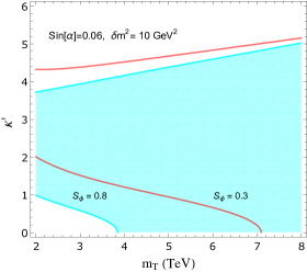
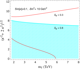
Figure 1: Regions satisfying the $S,T$ precision constraints at $99\%$ C.L. for the bi-doublet mixing scenario, with the left one for $SU(6)/SO(6)$ and the right one for $SU(6)/Sp(6)$. The cyan region is for $\sin\phi_{L}=0.8$ and the region between the two red lines are for $\sin\phi_{L}=0.3$.

4.2 SU(6)/Sp(6)

As we can see from Eq.(165-166), the $\kappa$ and $\kappa^{\prime}$ terms in the SU(6)/Sp(6) case generate the same interactions between the components fields in the bi-doublet and one singlet $T_{2}$ (in $\psi_{A}$) or $T_{3}$ (in $\psi_{1}$). For simplicity, we take the degenerate limit $m_{T_{2}}=m_{T_{3}}=M$, which gives:

$$\Delta T_{\rm mis} = \frac{N_{c}\sin^{2}\phi_{L}}{16\pi\sin^{2}\theta_{W}\cos^{2}\theta_{W}}\left[\frac{\kappa^{\prime 2}+2\kappa^{2}}{24}\sin^{2}\alpha\Big{[}\theta_{+}(y_{M},y_{b})-\theta_{+}(y_{M},y_{t})\Big{]}\right.$$ (141)

$$- \left.2\sin^{2}\frac{\alpha}{2}\theta_{+}(y_{t},y_{b})+\left(2\sin^{2}\frac{\alpha}{2}-\frac{\kappa^{\prime 2}+2\kappa^{2}}{24}\sin^{2}\alpha\right)\right.$$

$$\times \left.\Big{[}(y_{t}-y_{b})\left(\log\frac{\Lambda^{2}}{m^{2}_{Z}}-\frac{1}{2}\right)-2(y_{t}\log y_{t}-y_{b}\log y_{b})\Big{]}\right]\,.$$

This contribution enjoys the same structure as in the minimal SU(4)/Sp(4). For $\Delta S_{\rm mis}$, we obtain:

$$\Delta S_{\rm mis} = \Delta S_{div}-\frac{N_{c}\sin^{2}\alpha}{2\pi}\Big{[}\frac{\kappa^{\prime 2}+2\kappa^{2}}{24}\left[\sin^{2}\phi_{L}\chi_{+}(y_{t},y_{M})+(\cos^{2}\phi_{L}+1)\chi_{+}(y_{T},y_{M})\right]$$ (142)

$$+ \frac{\kappa^{\prime 2}+2\kappa^{2}}{12}\cos\phi_{L}\left[\chi_{-}(y_{T},y_{M})-\psi_{-}(y_{T},y_{M})\right]$$

with

$$\Delta S_{div} = \frac{N_{c}}{2\pi}\Big{[}\frac{8}{3}(2\sin^{2}\frac{\alpha}{2}-\frac{\kappa^{\prime 2}+2\kappa^{2}}{24}\sin^{2}\alpha)\left(\log\frac{\Lambda^{2}}{m^{2}_{Z}}-\frac{7}{6}\right)+\frac{\kappa^{\prime 2}+2\kappa^{2}}{36}\sin^{2}\alpha$$ (143)

$$+ \sin^{2}\phi_{L}\Big{[}\left(\frac{2}{3}\sin^{2}\frac{\alpha}{2}-\frac{\kappa^{\prime 2}+2\kappa^{2}}{48}\sin^{2}\alpha\right)\left(\frac{1}{3}-\frac{1}{3}\log y_{t}^{2}\right)-\frac{2}{3}\sin^{2}\frac{\alpha}{2}\Big{]}$$

$$+ \left(\cos^{2}\phi_{L}+1\right)\left(\frac{2}{3}\sin^{2}\frac{\alpha}{2}-\frac{\kappa^{\prime 2}+2\kappa^{2}}{48}\sin^{2}\alpha\right)\left(\frac{1}{3}-\frac{1}{3}\log y_{T}^{2}\right)$$

$$+ 2\left(\frac{10}{3}\sin^{2}\frac{\alpha}{2}-\frac{\kappa^{\prime 2}+2\kappa^{2}}{16}\sin^{2}\alpha\right)\left(\frac{1}{3}-\frac{1}{3}\log y_{M}^{2}\right)\Big{]}\,.$$

In analogy to the SU(6)/SO(6) case, $\Delta S_{\rm mis}$ can be estimated in the limit of $\sin\phi_{L}=0$ as:

$$\Delta S_{mis} = \frac{4N_{c}}{3\pi}\left(2\sin^{2}\frac{\alpha}{2}-\frac{\kappa^{\prime 2}+2\kappa^{2}}{24}\sin^{2}\alpha\right)\left(\log\frac{\Lambda^{2}}{m^{2}_{T}}-\frac{2}{3}\right)\,,$$ (144)

which is consistent with Eq. (140) with the coefficient difference originating from the representation of the top partners. Note that the divergence of $\Delta T_{\rm mis}$ and $\Delta S_{\rm mis}$ simultaneously vanish at the point $\sqrt{\kappa^{\prime 2}+2\kappa^{2}}=2\sqrt{3}/\cos\frac{\alpha}{2}$.

4.3 EWPT bounds

We performed a $\chi^{2}$ analysis for the parameter space spanned by $(\kappa,\kappa^{\prime},m_{T},\sin\phi_{L},\sin\alpha)$ in the two SU(6) models, using the EW precision data provided in the Particle Data Group (2022) Workman:2022ynf . In the bi-doublet mixing scenario, the positive contribution from $\Delta T_{mis}$ can be large enough to compensate the negative one from $\Delta T_{h}$. The plots in Figure 1 display the regions permitted by the $S$ and $T$ bounds by assuming $U=0$. The cyan band for $\sin\phi_{L}=0.8$ and the region between the two red lines for $\sin\phi_{L}=0.3$ are allowed by EWPO at $99\%$ C.L.. In fact, the patterns in two plots are mainly determined by $\Delta T_{mis}$ as the $\kappa^{\prime 2}$ and $(\kappa^{\prime 2}+2\kappa^{2})$ contributions have opposite signs in the two models. We find that, in order to allow $\kappa^{\prime}=0$ in the region of $m_{T}\sim$ a few TeV, a small symmetry breaking angle is preferred for the SU(6)/SO(6) model. Instead, in the SU(6)/Sp(6) model, the $\sin\alpha$ can be of order $0.1$ and smaller under the EWPO constraint. In Figure 1, we projected the EW bounds either on the $(\kappa^{\prime},m_{T})$ plane (left panel) or on the $(\sqrt{\kappa^{\prime 2}+2\kappa^{2}},m_{T})$ plane (right panel). Both plots show that with a larger $\sin\phi_{L}\sim 0.8$, the lower bound for the top partner can be relieved.

5 pNGB Dark Matter

Model	DM	Partner	$\tilde{y}_{L}$	$\tilde{y}_{R}$	$\lambda_{t}$	$a_{V}$
A	$\eta_{2}$	$\tilde{T}_{1}$	$i\frac{m_{T}}{2\sqrt{2}f}\sin 2\phi_{L}\sin 2\alpha$	$-iy_{d}\frac{m_{t}}{v}\frac{1}{\sin\phi_{L}}$	$\frac{1}{2}(1+\cos^{2}\phi_{L})$	$\frac{1}{2}\sin^{2}\alpha$
B	$\frac{\eta_{3}+i\eta_{4}}{\sqrt{2}}$	$\tilde{X}_{\frac{2}{3}}$	$\frac{m_{T}}{4\sqrt{2}f}\sin 2\phi_{L}\sin\alpha$	$\frac{\sqrt{2}m_{t}}{v}\frac{1}{\sin\phi_{L}}$	$\frac{1}{4}\cos^{2}\phi_{L}$	$3\sin^{2}\left(\frac{\alpha}{2}\right)$
	$\frac{\eta_{3}-i\eta_{4}}{\sqrt{2}}$	$\tilde{Y}_{\frac{2}{3}}$	$-\frac{m_{T}}{4\sqrt{2}f}\sin 2\phi_{L}\sin\alpha$	$-\frac{\sqrt{2}m_{t}}{v}\frac{1}{\sin\phi_{L}}$

Table 4: The couplings relevant to DM annihilation in Model A ($SU(6)/SO(6)$ CHM) and Model B ($SU(6)/Sp(6)$ CHM) for the bi-doublet mixing scenario, with $y_{d}=\frac{4R_{S2}}{\sqrt{3}R_{S1}-\sqrt{2}R_{S2}}$. In the 3rd row, the partner is a $Z_{2}$-odd heavy quark that mediates the interaction with a scalar DM and SM tops.

Due to the existence of a dark parity, the odd pNGBs $(S,H_{2})$ and the top partners $\tilde{T}$ in the composite inert Higgs model constitute the dark sector. In this paper, we consider the scenario of $m_{\tilde{T}}\gg m_{H_{2}}>m_{S}$, so that the singlet $S$ is the DM candidate. The rationale is the inert odd $H_{2}$ would most likely be excluded by direct detection bounds, due to a large Z boson coupling. The parity-odd scalars $H_{2}$ and $S$ were kept in a thermal equilibrium with the SM particles in the early universe and froze out as the temperature drops to $T_{f}\sim m_{S}/25$. When the mass difference between the doublet $H_{2}$ and singlet $S$ is large enough, the co-annihilation effect will be suppressed by $e^{-(m_{H_{2}}-m_{S})/T_{f}}$. Hence for $m_{H_{2}}>1.2\,m_{S}$, it is adequate to consider just the singlet annihilation. The Lagrangian relevant to the DM phenomenology is:

$$\mathcal{L}\supset - C_{hS}\,hS^{\dagger}S-a_{t}\frac{m_{t}}{v}\,h\bar{t}t-\tilde{y}_{L}\,\bar{t}_{L}\tilde{T}_{R}S-\tilde{y}_{R}\,\bar{t}_{R}\tilde{T}_{L}S+\lambda_{t}\frac{m_{t}}{f^{2}}S^{\dagger}S\bar{t}_{L}t_{R}+{\rm h.c.}$$ (145)

$$+ \frac{2m_{W}^{2}}{v}\left(h\cos\alpha-\frac{a_{V}}{v}S^{\dagger}S\right)\left(W^{+\mu}W^{-}_{\mu}+\frac{Z^{\mu}Z_{\mu}}{2\cos^{2}\theta_{W}}\right)$$

$$+ \frac{g_{2}}{4\cos\theta_{W}}\left(1-\cos\alpha\right)Z_{\mu}S^{\dagger}i\overset{\leftrightarrow}{\partial^{\mu}}S+Z_{\mu}\bar{q}\gamma^{\mu}\left(g_{v,q}-g_{a,q}\gamma_{5}\right)q\,,$$

with $a_{t}\simeq 1-\mathcal{O}(\sin^{2}\alpha)$, $g_{v,q}=\frac{g_{2}}{2\cos\theta_{W}}\left(T_{L}^{3}-2Q_{q}\sin^{2}\theta_{W}\right)$ and $g_{a,q}=\frac{g_{2}}{2\cos\theta_{W}}T_{L}^{3}$. Note that the DM is a real scalar singlet $S=\eta_{2}$ in SU(6)/SO(6) and a complex one $S=\frac{1}{\sqrt{2}}(\eta_{3}+i\eta_{4})$ in SU(6)/Sp(6). The $Z$ coupling to DM only exists for the complex singlet, and it is proportional to $(1-\cos\alpha)$ via the EW misalignment effect. The $S^{\dagger}S\bar{t}t$ term is connected to the generation of top quark mass and derived by expanding the trace part in Eq.(51) till the $1/f^{2}$ order. In the mass basis, the coefficient of this quartic term can be expressed in the form of $\lambda_{t}\frac{m_{t}}{f^{2}}$, that matches the structure derived from an EFT approach in Cai:2020njb . In fact we can comprehend this operator as the effect of integrating out the even top partners in $\Psi_{A}$ that mix with SM tops. In Table 4, we report the dark Yukawa couplings $\tilde{y}_{L,R}$ from the bi-doublet mixing scenario and the quartic couplings $(\lambda_{t},a_{V})$ in the two models. For the right-handed top spurion in SU(6)/SO(6), we set $R_{S1}=0,R_{S2}=1$ for a $\tilde{y}_{R}$ of $\mathcal{O}(1)$. Since $m_{t}$ is generated collectively by the left and right handed pre-Yukawa spurions, two couplings $\tilde{y}_{L,R}$ are present in the Lagrangian to couple the DM with the dark top partners. This feature extends the simplified vector-like quark portal DM model, where only one chiral (either left or right) Yukawa coupling is taken into account Giacchino:2013bta ; Cai:2018upp ; Colucci:2018vxz .

The Higgs portal coupling $C_{hS}$ is generated by the effective potential for the pNGBs and it depends on all the parameters in the underlying theory that break the global symmetries of the strong sector. In principle, the numerical values of this coupling need to be consistent with the non-tachyon condition (i.e. $m^{2}_{\rm pNGB}>0$) and with the stability of the dark parity (i.e. the absence of a VEV for the dark pNGBs) Cacciapaglia:2019ixa ; Cai:2020njb . As this exercise is strongly dependent on the details of the model, general and assumption-free bounds cannot be obtained and we will consider $C_{hS}$ as a free positive parameter with a reminder that over large or small values may be unphysical. Assuming the shift symmetry is dominantly broken with dark top partners running in the loop, one would expect $C_{hS}$ to be of the same order of the Higgs quartic times its VEV, i.e. $C_{hS}\sim\lambda_{h^{4}}v\sim 20$ GeV, as the Higgs mass is generated by the same spurions. However, this value should not be too large to conflict with DM direct detection bounds. Nevertheless, the DM candidate is not strictly correlated to the Higgs dynamics. With the cancellation from different contributions, values of $C_{hS}$ can be in a few GeV and even smaller in corners of the parameter space, that agrees with Ref. Balkin:2017aep for instance.

In this paper we will consider the DM annihilation $S^{\dagger}S\to\bar{t}t,W^{+}W^{-},ZZ$, that is justified when the mass region of interest is $2m_{S}<m_{t}+m_{T}$. The main focus of this work is on the $\bar{t}t$ channel, where the top partners directly contribute. The $WW$ and $ZZ$ channels are included as a comparison and to prove that the $tt$ channel dominates. The $hh$ channel is expected to contribute at the same order as $WW$ and $ZZ$ ones, however it receives model-dependent contributions from the pNGB potential. Hence, to keep the focus on the top partners, we do not include it explicitly and consider its effect as an $\mathcal{O}(1)$ uncertainty on the $WW+ZZ$ channels. Note that the $(\kappa,\kappa^{\prime})$ terms are neglected as well because they only entail the derivative couplings of DM at the leading order. But non-zero $(\kappa,\kappa^{\prime})$ can make the parameter space more natural under the EWPO constraint and have impact on the fractions of DM annihilation into $\bar{t}t$ and di-bosons.

5.1 Relic density computation

The DM relic density is determined by the thermal average of the annihilation cross section times the velocity $\langle\sigma v\rangle$, expanded in terms of $v_{rel}$. We can first calculate the un-averaged $\sigma v$ by summing over all the kinematically allowed channels:

$$\sigma v=\sum_{i,j}\frac{k_{ij}}{32\pi^{2}s}\frac{1}{S_{ij}}\int d\Omega|{\cal{M}}_{ij}|^{2}\,,$$ (146)

with $$k_{ij}=\left[1-\frac{(m_{i}+m_{j})^{2}}{s}\right]^{1/2}\left[1-\frac{(m_{i}-m_{j})^{2}}{s}\right]^{1/2}\,,$$ (147)

where $S_{ij}$ is a symmetric factor for identical final states and $s=E_{tot}^{2}$ is the Mandelstam variable, with $E_{tot}$ being the total energy in the center of mass frame. Due to the derivative coupling of $Z$-$S^{\dagger}$-$S$, its cross section is proportional to $(p_{S^{\dagger}}-p_{S})^{2}=-(s-4m_{S}^{2})$. Hence in the s-wave limit, the Z-portal interaction does not contribute to relic density. We will focus on the top Yukawa and Higgs mediating channels. Under the s-wave approximation, the thermal average of $\langle\sigma v\rangle_{\bar{t}t}$ in the two SU(6) models is:

$$\langle\sigma v\rangle_{\bar{t}t} = \frac{3M^{2}}{4\pi\left(M^{2}+m_{S}^{2}-m_{t}^{2}\right)^{2}}\left(1-\frac{m_{t}^{2}}{m_{S}^{2}}\right)^{\frac{3}{2}}\Big{[}2\tilde{y}_{L}\tilde{y}_{R}^{*}+\frac{m_{t}}{M}\Big{[}|\tilde{y}_{L}|^{2}+|\tilde{y}_{R}|^{2}$$ (148)

$$+ \beta_{S}\Big{(}\lambda_{t}\frac{4m_{S}^{2}-m_{h}^{2}}{f^{2}}-\frac{C_{hS}}{v}\Big{)}\frac{M^{2}+m_{S}^{2}-m_{t}^{2}}{4m_{S}^{2}-m_{h}^{2}}\Big{]}\Big{]}^{2}\,,$$

with $\beta_{S}=2$ for a real scalar ($S^{\dagger}=S$) and $\beta_{S}=1$ for a complex scalar, where the difference shows up in the Higgs mediating channel. From Table 4 we can see that $\tilde{y}_{L}\tilde{y}_{R}^{*}$ can be of the same order as $\frac{m_{t}}{M}|\tilde{y}_{R}|^{2}$, while the $\frac{m_{t}}{M}|\tilde{y}_{L}|^{2}$ term is negligible. Note that for $C_{hS}=0$ and in the limit of $M\gg m_{S}\gg m_{f}$, our results agree with the calculation in Ref. Boehm:2003hm . In particular, two dark top partners ($\tilde{X}_{\frac{2}{3}}$, $\tilde{Y}_{\frac{2}{3}}$) participate in the annihilation of the complex scalar DM in SU(6)/Sp(6), which is equivalent to the $t$ and $u$ channels for the real scalar DM in SU(6)/SO(6). Thus in our models, there is no $\frac{1}{4}$ factor difference among the real and complex cases in the top partner mediating cross section as pointed out by Boehm:2003hm .

Similarly for the di-boson annihilation channels, at the leading order, the thermal average of $\langle\sigma v\rangle_{VV}$ with $V=W,Z$ is:

$$\langle\sigma v\rangle_{WW} = \frac{\pi\alpha_{E}^{2}\left(4\frac{m_{S}^{4}}{m_{W}^{4}}-4\frac{m_{S}^{2}}{m_{W}^{2}}+3\right)\beta_{S}^{2}}{8m_{S}^{2}s_{W}^{4}\left(4m_{S}^{2}-m_{h}^{2}\right)^{2}}\sqrt{1-\frac{m_{W}^{2}}{m_{S}^{2}}}$$ (149)

$$\times \left(a_{V}\left(4m_{S}^{2}-m_{h}^{2}\right)-C_{hS}\,v\cos(\alpha)\right)^{2}\,,$$

and

$$\langle\sigma v\rangle_{ZZ} = \frac{\pi\alpha_{E}^{2}\left(4\frac{m_{S}^{4}}{m_{Z}^{4}}-4\frac{m_{S}^{2}}{m_{Z}^{2}}+3\right)\beta_{S}^{2}}{16m_{S}^{2}s_{W}^{4}c_{W}^{4}\left(4m_{S}^{2}-m_{h}^{2}\right)^{2}}\sqrt{1-\frac{m_{Z}^{2}}{m_{S}^{2}}}$$ (150)

$$\times \left(a_{V}\left(4m_{S}^{2}-m_{h}^{2}\right)-C_{hS}\,v\cos(\alpha)\right)^{2}\,.$$

Without the Higgs portal interaction, the di-boson annihilation rate is roughly proportional to $m_{S}^{2}$ and becomes larger for heavier DM. Assuming $C_{hS}=0$ and $m_{S}\sim 200$ GeV, we obtain $\langle\sigma v\rangle_{WW}+\langle\sigma v\rangle_{ZZ}\sim a_{V}^{2}\beta_{S}^{2}\times 2.0\times 10^{-23}\mbox{cm}^{3}/s$. For a light DM and $a_{V}<10^{-2}$, the di-boson channel alone can not saturate the relic density.

From the perspective of the Boltzmann equation, the freeze-out epoch is fixed by the condition that the DM particles stop to track the equilibrium distribution. By defining $x_{f}=\frac{m_{S}}{T_{f}}$, this freeze-out temperature is determined as:

$$x_{f}=\log\left[0.038c(c+2)\langle\sigma v_{\rm tot}\rangle\frac{g_{S}m_{S}M_{\rm PL}}{\sqrt{g_{*}x_{f}}}\right]$$ (151)

with $c=\sqrt{2}-1$, $M_{PL}=1.22\times 10^{19}$ GeV and $g_{*}\sim 100$. Since $g_{S}$ counts the internal DM degrees of freedom, we set $g_{S}=2$ for a complex scalar and $g_{S}=1$ for a real scalar. For a total cross section $\langle\sigma v\rangle_{\rm tot}\sim 2\times 10^{-26}cm^{3}/s$ and $m_{S}\sim 10^{2}-10^{3}$GeV, the freeze-out condition gives $x_{f}\simeq 20-25$. The relic density can be estimated using the following formula:

$$\Omega h^{2}\approx g_{S}\frac{1.07\times 10^{9}~{}\rm{GeV}^{-1}}{\sqrt{g_{*}(x_{f})}M_{\rm PL}\langle\sigma v_{\rm tot}\rangle/x_{f}}\,.$$ (152)

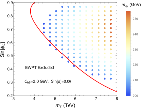
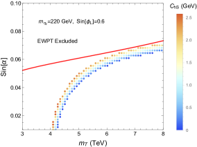
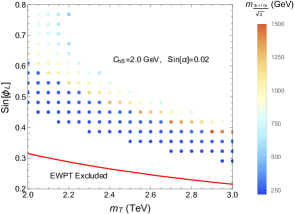
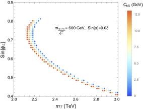
Figure 2: The colored regions provide the correct relic density $\Omega h^{2}=0.12\pm 0.002$, and satisfy the direct detection constraint, with the upper panels for SU(6)/SO(6) and the lower panels for SU(6)/Sp(6). The red line is the EWPO bound at $99\%$ C.L. with $\kappa=\kappa^{\prime}=0$.

5.2 Direct detection constraint

To evaluate the spin-independent DM-nucleon scattering, we can start with the effective Lagrangian in terms of gluons and quarks:

$$\mathcal{L}_{eff} = C_{q}\sum\limits_{q=u,d,s}\,m_{q}S^{\dagger}S\bar{q}q+\frac{\alpha_{s}}{4\pi}\left(4\,C_{S}^{g}-C_{q}-\frac{\lambda_{t}}{3f^{2}}\right)S^{\dagger}SG^{A\mu\nu}G^{A}_{\mu\nu}$$ (153)

$$+ \sum\limits_{q=u,d}C_{Z}^{q}S^{\dagger}i\overset{\leftrightarrow}{\partial_{\mu}}S\bar{q}\gamma^{\mu}q\,,$$

where the vector interaction term is obtained by integrating out the $Z$ gauge boson with

$$C_{Z}^{q}=\frac{g_{2}\,g_{v,q}}{4m_{Z}^{2}\cos\theta_{W}}\left(1-\cos\alpha\right)\,,$$ (154)

and the vector-axial interaction is not listed as its contribution to the spin-independent cross section is velocity suppressed. For the gluon operator in the first line of Eq.(153), the $C_{q}$ term is generated from the Higgs portal triangle diagram with heavy quarks $(c,t,b)$ running in the loop, while $C_{S}^{g}$ comes from the top partner box diagram. These Wilson coefficients in the first line are given by Hisano:2010ct ; Cheng:2012qr ; Hisano:2015bma :

$$C_{q}=\frac{C_{hS}}{vm_{h}^{2}}\,,\quad C_{S}^{g}=-\frac{1}{24\beta_{S}}\left[\frac{\left(\tilde{y}_{L}^{2}+\tilde{y}_{R}^{2}\right)m_{S}^{2}}{(M^{2}-m_{S}^{2})^{2}}+\frac{4\tilde{y}_{L}\tilde{y}_{R}M}{(M^{2}-m_{S}^{2})m_{t}}\right]\,,$$ (155)

where $\beta_{S}$ takes into account the difference of mediators in two SU(6) models. Then the coupling $f_{p,n}$ for DM interacting with protons or neutrons are factorized as the Wilson coefficients in Eq.(153) times the nucleon matrix elements. Expanding in the non-relativistic limit, the spinor structures inside $\langle N|\bar{q}\gamma^{\mu}q|N\rangle$, $\langle N|\bar{q}q|N\rangle$ and $\langle N|G^{A}_{\mu\nu}G^{A\mu\nu}|N\rangle$ are the same. Hence the operators from Eq.(153) contribute to $f_{p,n}$ in an interference way:

$$f_{p,n}=\sum\limits_{q=u,d,s}C_{q}\,f^{(p,n)}_{q}+\frac{2}{9}\,\left(C_{q}+\frac{\lambda_{t}}{3f^{2}}-4\,C_{S}^{g}\right)f_{TG}^{(p,n)}\pm\frac{2m_{S}}{m_{N}}C_{Z}^{(p,n)}\,,$$ (156)

where the last term is from the $Z$ portal in the complex scalar DM scenario, with the sign $\pm$ standing for the scattering of a particle or anti-particle DM. Note that $m_{N}$ is the nucleon mass and the form factors are $C_{Z}^{p}=2C_{Z}^{u}+C_{Z}^{d}$, $C_{Z}^{n}=C_{Z}^{u}+2C_{Z}^{d}$. For $C_{S}^{g}=C_{Z}^{(p,n)}=0$, Eq.(156) goes back to the pure Higgs portal scenario Cai:2020njb . And the matrix elements related to Higgs portal are defined by Drees:1993bu :

$$f_{q}^{(p,n)}=\frac{m_{q}}{m_{N}}\langle N|\bar{q}q|N\rangle\,,\quad f_{TG}^{p,n}=-\frac{9}{8\,m_{N}}\langle N|\frac{\alpha_{s}}{\pi}G^{A}_{\mu\nu}G^{A\mu\nu}|N\rangle$$ (157)

Operating the nucleon states on the trace of the stress energy tensor gives the following relation Shifman:1978zn :

$$f_{TG}^{(p,n)}=\left(1-\sum\limits_{q=u,d,s}f_{q}^{(p,n)}\right)\,.$$ (158)

where $f_{q}^{(p,n)}$ is the quark mass fraction that can be calculated by lattice simulation or chiral perturbation theory, and we will use the values listed in Hisano:2015bma . Finally, the spin-independent cross section is

$$\sigma_{\rm SI}=\frac{m_{N}^{2}\beta_{S}^{2}}{4\pi m_{S}^{2}}\left(\frac{m_{N}m_{S}}{m_{N}+m_{S}}\right)^{2}\frac{(Zf_{p}+(A-Z)f_{n})^{2}}{A^{2}}\,.$$ (159)

As indicated in Eq.(156), the Z-portal interaction of particle and anti-particle DMs is either constructive or deconstructive with the Higgs portal one in the DM-nucleon coupling $f_{p,n}$. For the complex DM in SU(6)/Sp(6) CHM, we need to average over this two effects, i.e. $\sigma_{\rm SI}^{tot}=\frac{1}{2}\left(\sigma_{\rm SI}+\bar{\sigma}_{\rm SI}\right)$. The measurement of $\sigma_{\rm SI}$ at the underground detectors XENON:2018voc ; Cui:2017nnn ; Akerib:2016vxi ; PandaX-4T:2021bab ; LZ:2022ufs will impose constraint on $(m_{S},f_{p,n})$. With $m_{T}>2$ TeV and $m_{S}\in(0.2,1.5)$ TeV, the dark top partner induced $\sigma_{\rm SI}$ normally is $<10^{-48}\,\mbox{cm}^{2}$, several orders of magnitude smaller than the upper limit. Hence, the direct detection mainly constrains the parameters related to the Higgs or Z-portal interactions, i.e. $(C_{hS},m_{S})$ in SU(6)/SO(6) CHM and $(C_{hS},m_{S},\sin\alpha)$ in SU(6)/Sp(6) CHM. For the complex DM, the Z-portal interaction places a stringent upper bound on $\sin\alpha$. Using the latest LUX-ZEPLIN measurement LZ:2022ufs , we find with $C_{hS}=0$ and $m_{S}\in(0.2,1.5)$TeV, the upper limit of $\sin\alpha$ in SU(6)/Sp(6) CHM falls in the range of $(0.024,0.04)$. Adding the Higgs coupling $C_{hS}$ will further reduce the allowed $\sin\alpha$ value. The benefit to include odd top partners is that the dark Yukawa interaction brings in sufficient additional annihilation rate that compensates the smallness of Higgs portal one, while is not sensitive to the direct detection in the preferred $(m_{T},m_{S})$ parameter space. Therefore, the dark top partners in fact relieve the tension in a Higgs portal DM model.

5.3 Combined analysis

There are 5 independent parameters in our DM models, i.e. $(C_{hS},m_{S},m_{T},\sin\alpha,\sin\phi_{L})$, where the last 3 ones are related to EWPOs. A comprehensive analysis is conducted to find the viable parameter space. However we will not include the bound from indirect detection, e.g. the gamma rays observed in dwarf spheroidal galaxies or the Galactic Center. The signals normally impose constraint on the low DM mass scenario ($\lesssim 100$ GeV) Ackermann:2015zua ; Hoof:2018hyn . A recent interpolation pushed up the bounds near several hundred GeV for the $\bar{b}b$, $WW$, $ZZ$ channels, but lack of $\bar{t}t$ information Abazajian:2020tww . Note that our analyses in both CHMs are restricted to a small $\sin\alpha$ and this results in $SS\to\bar{t}t$ playing a dominant role with more than $90\%$ contribution to the DM annihilation. For the DM mass in $(0.2,1.5)$ TeV, the upper limit on $\langle\sigma v\rangle_{\bar{t}t}$ is around $5.0\times 10^{-26}\rm{cm}^{3}s^{-1}$ from the 11 years of Fermi-LAT observations Hoof:2018hyn , with almost no constraint on the parameter space.

In Figure 2, we require the scalar DM to accommodate the correct relic density $0.118<\Omega h^{2}<0.122$ Aghanim:2018eyx and simultaneously satisfy the constraints from the direct detection and EWPOs. In addition, collider experiments impose direct constraints on the dark top partners and the $(T_{X},X)$ in the $Z_{2}$-even bi-doublet ATLAS:2018ziw ; ATLAS:2018alq ; CMS:2018zkf . Henceforth, the points in the plots need to satisfy $M=m_{T}\cos\phi_{L}>1.3$ TeV. The upper panels refer to SU(6)/SO(6): In Figure 2(a), we set $C_{hS}=2$ GeV, and the relic density dominantly comes from the top partner channel. We can see that the DM mass is constrained to be $200\lesssim m_{\eta_{2}}\lesssim 255$ GeV for $m_{T}\leq 8$ TeV. A lower DM mass from this region will demand for smaller $\sin\phi_{L}$ and $m_{T}$, thus is excluded by EWPOs. Corresponding results for SU(6)/Sp(6) are displayed in the lower panels. For this case, the allowed value of $\sin\alpha$ derived from the direct detection strictly constrains the lower limit of DM mass, while the bound from EWPO is relatively loose. In Figure 2(c) with $C_{hS}=2$ GeV, $\sin\alpha=0.02$, the DM mass populates in a wide range $200\lesssim m_{\frac{\eta_{3}+i\eta_{4}}{\sqrt{2}}}\lesssim 1500$ GeV. Increasing $\sin\alpha$ will cut off the lower mass region. The impacts of $C_{hS}$ for two models are visualized in Figure 2(b) and 2(d), with its value limited by the direct detection bound. From Eq.(148), we find that a positive $C_{hS}$ makes the Higgs portal deconstructive with the top partner channel, hence requires a lighter top partner. The narrow bands from the variation of $C_{hS}$ indicate that the Higgs portal only offers a subleading contribution.

6 Conclusion

Extending the global symmetries of composite Higgs models allow to accommodate for stable pNGBs, which can play the role of Dark Matter. In fundamental CHMs with real and pseudo-real realizations, this amounts to add the HC fermions that are odd under a $\mathbb{Z}_{2}$ dark parity. In return, odd resonances as condensations of HC fermions appear in all sectors of the theory. However for the complex realization of CHM, a simple $\mathbb{Z}_{2}$ for the HC fermions is not adequate as the conjugate operation plus internal flavor rotation might be involved.

Partial compositeness for the top quark mass generation plays a crucial role in this class of models. On one hand, the couplings of the elementary top fields must preserve the dark parity, hence imposing non-trivial constraints on the UV completions of the models. On the other hand, the presence of odd top partners relieves the tension of Higgs portal coupling with the direct detection.

We have considered in detail the role played by the dark top partners in two models based on fundamental dynamics, where the composite Higgs boson and Dark Matter stem from the cosets SU(6)/SO(6) and SU(6)/Sp(6). Following Ref. Cai:2022zqu , we considered the impact of electroweak constraints on the models. Furthermore, we studied the properties of the pNGB DM in the presence of the dark top partners. They enter as mediators for the annihilation of the DM candidate in the early Universe and at direct detection experiments. This effect can dominate over the Higgs mediated processes, with non-trivial interference effects taken into account. As a result, phenomenological constraints require the mass of the even top partner to be in the multi TeV regime, with viable masses above 4 TeV for SU(6)/SO(6) and lower to 2 TeV for SU(6)/Sp(6). These masses can only be directly probed at future high-energy hadronic colliders.

Appendix A EW gauge interaction

We will write down the EW gauge interactions with the top partners not rotated into the mass basis. In the $SU(6)/SO(6)$ CHM, the $\Psi_{A}$ gauge interaction includes a standard part:

$$Tr\left[\bar{\psi}_{A}\gamma^{\mu}\left(V_{\mu}\psi_{A}+\psi_{A}V_{\mu}^{T}\right)+g_{1}B_{\mu}^{0}\hat{X}\bar{\psi}_{A}\gamma^{\mu}\psi_{A}\right]$$ (160)

$$= \frac{g_{2}W^{+}_{\mu}}{\sqrt{2}}\left[\overline{\tilde{T}}\gamma^{\mu}\tilde{B}+\overline{\tilde{X}}\gamma^{\mu}\tilde{T}_{X}+\bar{T}\gamma^{\mu}B+\bar{X}\gamma^{\mu}T_{X}+\sqrt{2}\left(\bar{X}_{\frac{2}{3}}\gamma^{\mu}X_{-\frac{1}{3}}-\bar{X}_{\frac{5}{3}}\gamma^{\mu}X_{\frac{2}{3}}\right)\right]+h.c.$$

$$+ \frac{g_{2}W^{3}_{\mu}}{2}\Big{[}\overline{\tilde{T}}\gamma^{\mu}\tilde{T}-\overline{\tilde{B}}\gamma^{\mu}\tilde{B}+\overline{\tilde{X}}\gamma^{\mu}\tilde{X}-\overline{\tilde{T}}_{X}\gamma^{\mu}\tilde{T}_{X}+\bar{T}\gamma^{\mu}T-\bar{B}\gamma^{\mu}B+\bar{X}\gamma^{\mu}X-\bar{T}_{X}\gamma^{\mu}T_{X}$$

$$- 2\bar{X}_{-\frac{1}{3}}\gamma^{\mu}X_{-\frac{1}{3}}+2\bar{X}_{\frac{5}{3}}\gamma^{\mu}X_{\frac{5}{3}}\Big{]}+g_{1}B_{\mu}^{0}\Big{[}\frac{1}{6}\left(\overline{\tilde{T}}\gamma^{\mu}\tilde{T}+\overline{\tilde{B}}\gamma^{\mu}\tilde{B}+\bar{T}\gamma^{\mu}T+\bar{B}\gamma^{\mu}B\right)$$

$$+ \frac{7}{6}\left(\overline{\tilde{X}}\gamma^{\mu}\tilde{X}+\overline{\tilde{T}}_{X}\gamma^{\mu}\tilde{T}_{X}+\bar{X}\gamma^{\mu}X+\bar{T}_{X}\gamma^{\mu}T_{X}\right)+\frac{2}{3}\left(\bar{X}_{-\frac{1}{3}}\gamma^{\mu}X_{-\frac{1}{3}}+\bar{X}_{\frac{2}{3}}\gamma^{\mu}X_{\frac{2}{3}}+\bar{X}_{\frac{5}{3}}\gamma^{\mu}X_{\frac{5}{3}}\right)$$

$$- \frac{1}{3}\bar{Y}_{-\frac{1}{3}}\gamma^{\mu}Y_{-\frac{1}{3}}+\frac{2}{3}\bar{Y}_{\frac{2}{3}}\gamma^{\mu}Y_{\frac{2}{3}}+\frac{5}{3}\bar{Y}_{\frac{5}{3}}\gamma^{\mu}Y_{\frac{5}{3}}\Big{]}$$

with $V_{\mu}=g_{2}W_{\mu}^{i}T^{i}_{L}+g_{1}B_{\mu}^{0}T^{3}_{R}$. And the misaligned effect is separately encoded in $\delta E_{\mu}=E_{\mu}-V_{\mu}$. We can expand the relevant Lagrangian to obtain at the leading order:

$$Tr\left[\bar{\psi}_{A}\gamma^{\mu}\left(\delta E_{\mu}\psi_{A}+\psi_{A}\delta E_{\mu}^{T}\right)\right]\supset$$ (161)

$$-\frac{g_{2}\sin^{2}\left(\frac{\alpha}{2}\right)}{2}\Big{[}W_{\mu}^{1}\Big{[}\left(\overline{\tilde{B}}-\overline{\tilde{X}}\right)\gamma^{\mu}\left(\tilde{T}-\tilde{T}_{X}\right)+\left(\bar{B}-\bar{X}\right)\gamma^{\mu}\left(T-T_{X}\right)$$

$$-\sqrt{2}\left(\bar{X}_{\frac{2}{3}}\gamma^{\mu}\left(X_{\frac{5}{3}}-X_{-\frac{1}{3}}\right)+\bar{Y}_{\frac{2}{3}}\gamma^{\mu}\left(Y_{-\frac{1}{3}}-Y_{\frac{5}{3}}\right)\right)\Big{]}$$

$$+iW_{\mu}^{2}\Big{[}\left(\overline{\tilde{B}}+\overline{\tilde{X}}\right)\gamma^{\mu}\left(\tilde{T}-\tilde{T}_{X}\right)+\left(\bar{B}+\bar{X}\right)\gamma^{\mu}\left(T-T_{X}\right)$$

$$-\sqrt{2}\left(\bar{X}_{\frac{2}{3}}\gamma^{\mu}\left(X_{-\frac{1}{3}}+X_{\frac{5}{3}}\right)-\bar{Y}_{\frac{2}{3}}\gamma^{\mu}\left(Y_{-\frac{1}{3}}+Y_{\frac{5}{3}}\right)\right)\Big{]}$$

$$+ 2\Big{(}W_{\mu}^{3}-B_{\mu}^{0}\tan(\text{$\theta$w})\Big{)}\Big{[}\overline{\tilde{T}}\gamma^{\mu}\tilde{T}-\overline{\tilde{T}}_{X}\gamma^{\mu}\tilde{T}_{X}+\bar{T}\gamma^{\mu}T-\bar{T}_{X}\gamma^{\mu}T_{X}$$

$$-\bar{X}_{-\frac{1}{3}}\gamma^{\mu}X_{-\frac{1}{3}}+\bar{X}_{\frac{5}{3}}\gamma^{\mu}X_{\frac{5}{3}}+\bar{Y}_{-\frac{1}{3}}\gamma^{\mu}Y_{-\frac{1}{3}}-\bar{Y}_{\frac{5}{3}}\gamma^{\mu}Y_{\frac{5}{3}}\Big{]}\Big{]}\,,$$

The $\kappa^{\prime}$ term in Eq.(47) will also modify the gauge interactions:

$$Tr[\bar{\psi}_{A}d_{\mu}\gamma^{\mu}\psi_{A}]\supset$$ (162)

$$\frac{1}{8}g_{2}W_{1}^{\mu}\sin(\alpha)\left(\sqrt{2}\left(\overline{\tilde{B}}-\overline{\tilde{X}}\right)\gamma_{\mu}\tilde{T}_{1}-\left(\bar{B}+\bar{X}\right)\gamma_{\mu}\left(X_{\frac{2}{3}}+Y_{\frac{2}{3}}\right)\right.$$

$$+ \left.\sqrt{2}\bar{T}\gamma_{\mu}\left(X_{\frac{5}{3}}-Y_{-\frac{1}{3}}\right)+\sqrt{2}\bar{T}_{X}\gamma_{\mu}\left(Y_{\frac{5}{3}}-X_{-\frac{1}{3}}\right)\right)$$

$$+ \frac{i}{8}g_{2}W_{2}^{\mu}\sin(\alpha)\left(\sqrt{2}\left(\overline{\tilde{B}}+\overline{\tilde{X}}\right)\gamma_{\mu}\tilde{T}_{1}-\left(\bar{B}-\bar{X}\right)\gamma_{\mu}\left(X_{\frac{2}{3}}+Y_{\frac{2}{3}}\right)\right.$$

$$+ \left.\sqrt{2}\bar{T}\gamma_{\mu}\left(X_{\frac{5}{3}}+Y_{-\frac{1}{3}}\right)+\sqrt{2}\bar{T}_{X}\gamma_{\mu}\left(X_{-\frac{1}{3}}+Y_{\frac{5}{3}}\right)\right)$$

$$+ \frac{1}{8}g_{2}\left(W_{3}^{\mu}-B_{0}^{\mu}\tan(\text{$\theta$w})\right)\sin(\alpha)\left(\sqrt{2}\left(\overline{\tilde{T}}+\overline{\tilde{T}}_{X}\right)\gamma_{\mu}\tilde{T}_{1}+\sqrt{2}\bar{B}\gamma_{\mu}\left(X_{-\frac{1}{3}}+Y_{-\frac{1}{3}}\right)\right.$$

$$+ \left.\left(\bar{T}-\bar{T}_{X}\right)\gamma_{\mu}\left(X_{\frac{2}{3}}-Y_{\frac{2}{3}}\right)+\sqrt{2}\bar{X}\gamma_{\mu}\left(X_{\frac{5}{3}}+Y_{\frac{5}{3}}\right)\right)+h.c.\,$$

Note that because the charge operator $Q$ is conserved, only $W_{\mu}^{\pm}$ and $Z_{\mu}$ couplings are misaligned by the $\sin\alpha$ corrections.

Similarly for the $SU(6)/Sp(6)$ CHM, the Lagrangian of the covariant gauge interaction can split into the SM part plus the misalignment one as following:

$$Tr\left[\bar{\psi}_{A}\gamma^{\mu}\left(V_{\mu}\psi_{A}+\psi_{A}V_{\mu}^{T}\right)+g_{1}B_{\mu}^{0}\hat{X}\bar{\psi}_{A}\gamma^{\mu}\psi_{A}\right]$$ (163)

$$= \frac{g_{2}W^{+}_{\mu}}{\sqrt{2}}\left[\overline{\tilde{T}}\gamma^{\mu}\tilde{B}+\overline{\tilde{X}}\gamma^{\mu}\tilde{T}_{X}+\bar{T}\gamma^{\mu}B+\bar{X}\gamma^{\mu}T_{X}\right]+h.c.$$

$$+ \frac{g_{2}W^{3}_{\mu}}{2}\Big{[}\overline{\tilde{T}}\gamma^{\mu}\tilde{T}-\overline{\tilde{B}}\gamma^{\mu}\tilde{B}+\overline{\tilde{X}}\gamma^{\mu}\tilde{X}-\overline{\tilde{T}}_{X}\gamma^{\mu}\tilde{T}_{X}+\bar{T}\gamma^{\mu}T-\bar{B}\gamma^{\mu}B$$

$$+ \bar{X}\gamma^{\mu}X-\bar{T}_{X}\gamma^{\mu}T_{X}\Big{]}++g_{1}B_{\mu}^{0}\Big{[}\frac{1}{6}\left(\overline{\tilde{T}}\gamma^{\mu}\tilde{T}+\overline{\tilde{B}}\gamma^{\mu}\tilde{B}+\bar{T}\gamma^{\mu}T+\bar{B}\gamma^{\mu}B\right)$$

$$+ \frac{7}{6}\left(\overline{\tilde{X}}\gamma^{\mu}\tilde{X}+\overline{\tilde{T}}_{X}\gamma^{\mu}\tilde{T}_{X}+\bar{X}\gamma^{\mu}X+\bar{T}_{X}\gamma^{\mu}T_{X}\right)-\frac{1}{3}\bar{X}_{-\frac{1}{3}}\gamma^{\mu}X_{-\frac{1}{3}}+\frac{5}{3}\bar{X}_{\frac{5}{3}}\gamma^{\mu}X_{\frac{5}{3}}$$

$$+ \frac{2}{3}\left(\bar{X}_{\frac{2}{3}}\gamma^{\mu}X_{\frac{2}{3}}+\bar{Y}_{\frac{2}{3}}\gamma^{\mu}Y_{\frac{2}{3}}+\bar{T}_{1}\gamma^{\mu}T_{1}+\bar{T}_{2}\gamma^{\mu}T_{2}\right)$$

$$Tr\left[\bar{\psi}_{A}\gamma^{\mu}\left(\delta E_{\mu}\psi_{A}+\psi_{A}\delta E_{\mu}^{T}\right)\right]\supset$$ (164)

$$-\frac{g_{2}\sin^{2}\left(\frac{\alpha}{2}\right)}{2}\Big{[}\left(W_{\mu}^{1}-iW_{\mu}^{2}\right)\Big{[}\overline{\tilde{T}}\gamma^{\mu}\tilde{B}+\overline{\tilde{X}}\gamma^{\mu}\tilde{T}_{X}+\overline{\tilde{Y}}_{\frac{2}{3}}\gamma^{\mu}\tilde{X}_{-\frac{1}{3}}+\overline{\tilde{X}}_{\frac{5}{3}}\gamma^{\mu}\tilde{X}_{\frac{2}{3}}\Big{]}$$

$$+ \Big{[}W_{\mu}^{1}\left(\bar{B}+\bar{X}\right)\gamma^{\mu}\left(T_{X}+T\right)+iW_{\mu}^{2}\left(\bar{B}-\bar{X}\right)\gamma^{\mu}\left(T_{X}+T\right)\Big{]}+h.c.$$

$$+ \Big{(}W_{\mu}^{3}-B_{\mu}^{0}\tan(\text{$\theta$w})\Big{)}\Big{[}\overline{\tilde{T}}\gamma^{\mu}\tilde{T}-\overline{\tilde{B}}\gamma^{\mu}\tilde{B}+\overline{\tilde{X}}\gamma^{\mu}\tilde{X}-\overline{\tilde{T}}_{X}\gamma^{\mu}\tilde{T}_{X}+\overline{\tilde{X}}_{-\frac{1}{3}}\gamma^{\mu}\tilde{X}_{-\frac{1}{3}}$$

$$+ \overline{\tilde{X}}_{\frac{2}{3}}\gamma^{\mu}\tilde{X}_{\frac{2}{3}}-\overline{\tilde{X}}_{\frac{5}{3}}\gamma^{\mu}\tilde{X}_{\frac{5}{3}}-\overline{\tilde{Y}}_{\frac{2}{3}}\gamma^{\mu}\tilde{Y}_{\frac{2}{3}}-2\bar{T}_{X}\gamma^{\mu}T_{X}+2\bar{T}\gamma^{\mu}T\Big{]}\Big{]}$$

Finally the $\kappa^{\prime},\kappa$ terms in Eq.(47) from the CCWZ formalism can be expanded as:

$$Tr\left[\bar{\psi}_{A}\not{d}\ \psi_{A}\right]\supset$$ (165)

$$\frac{g_{2}\sin(\alpha)}{8\sqrt{3}}\Big{[}\sqrt{3}\left(W_{\mu}^{1}-iW_{\mu}^{2}\right)\left(\overline{\tilde{Y}}_{\frac{2}{3}}\gamma^{\mu}\tilde{B}+\overline{\tilde{X}}_{\frac{5}{3}}\gamma^{\mu}\tilde{T}_{X}-\overline{\tilde{T}}\gamma^{\mu}\tilde{X}_{-\frac{1}{3}}-\overline{\tilde{X}}\gamma^{\mu}\tilde{X}_{\frac{2}{3}}\right)$$

$$+ \sqrt{2}\Big{(}W_{\mu}^{1}\left(\bar{B}+\bar{X}\right)\gamma^{\mu}T_{2}+iW_{\mu}^{2}\left(\bar{B}-\bar{X}\right)\gamma^{\mu}T_{2}\Big{)}$$

$$+ \left(W_{\mu}^{3}-B_{\mu}\tan(\text{$\theta$w})\right)\Big{(}\sqrt{3}\Big{(}\overline{\tilde{B}}\gamma^{\mu}\tilde{X}_{-\frac{1}{3}}+\overline{\tilde{T}}_{X}\gamma^{\mu}\tilde{X}_{\frac{2}{3}}$$

$$+ \overline{\tilde{T}}\gamma^{\mu}\tilde{Y}_{\frac{2}{3}}+\overline{\tilde{X}}_{\frac{5}{3}}\gamma^{\mu}\tilde{X}\Big{)}+\sqrt{2}\left(\bar{T}-\bar{T}_{X}\right)\gamma^{\mu}T_{2}\Big{)}+h.c.\,$$

$$Tr[\bar{\psi}_{A}d_{\mu}\gamma^{\mu}\psi_{1}]+h.c. \supset \frac{g_{2}\sin(\alpha)}{4\sqrt{3}}\Big{[}W^{1}_{\mu}\left(\bar{B}+\bar{X}\right)\gamma^{\mu}T_{3}+iW^{2}_{\mu}\left(\bar{B}-\bar{X}\right)\gamma^{\mu}T_{3}$$ (166)

$$+ \left(W^{3}_{\mu}-B^{0}_{\mu}\tan(\text{$\theta$w})\right)\left(\bar{T}-\bar{T}_{X}\right)\gamma^{\mu}T_{3}\Big{]}+h.c.\,$$

Appendix B DM Yukawa interaction

We will derive the couplings between the odd pNGB and dark top partners generated from the partial compositeness in Eq.(51). For the $SU(6)/SO(6)$ CHM, we find that:

$$\mathcal{L}_{\eta_{2}} = -i\eta_{2}y_{L}\bar{t}_{L}\left(\sin 2\alpha Q_{A1}\tilde{T}_{1}+\sqrt{2}Q_{S2}\left(\tilde{T}\cos^{2}\frac{\alpha}{2}-\tilde{T}_{X}\sin^{2}\frac{\alpha}{2}\right)\right)$$ (167)

$$+ \frac{i}{2}\eta_{2}y_{R}\bar{t}_{R}\left(\sin\alpha R_{A4}\left(\tilde{T}_{X}+\tilde{T}\right)-\tilde{T}_{1}\left(\sin^{2}\alpha(\sqrt{6}R_{S1}-2R_{S2})+4R_{S2}\right)\right)$$

$$- i\eta_{2}y_{L}\bar{b}_{L}\tilde{B}\sqrt{2}\cos\alpha Q_{S2}+h.c.$$

$$\mathcal{L}_{H_{0}/A_{0}} = -\frac{1}{2}H_{0}y_{L}\bar{t}_{L}\left(\sqrt{2}Q_{A1}\left(\sin 2\alpha\left(\tilde{T}-\tilde{T}_{X}\right)+\sin\alpha\left(\tilde{T}_{X}+\tilde{T}\right)\right)+2Q_{S2}\tilde{T}_{1}\right)$$ (168)

$$+ \frac{1}{2}H_{0}y_{R}\bar{t}_{R}\left(\cos^{2}\alpha(\sqrt{3}R_{S1}-\sqrt{2}R_{S2})+2\sqrt{2}R_{S2}\right)\left(\tilde{T}-\tilde{T}_{X}\right)$$

$$+ \frac{i}{2}A_{0}y_{L}\bar{t}_{L}\left(\sqrt{2}\sin\alpha Q_{A1}\left(\tilde{T}-\tilde{T}_{X}\right)+2\cos\alpha Q_{S2}\tilde{T}_{1}\right)$$

$$- \frac{i}{2}A_{0}y_{R}\bar{t}_{R}\left(\sqrt{2}\sin\alpha R_{A4}\tilde{T}_{1}-\left(\sqrt{3}R_{S1}+\sqrt{2}R_{S2}\right)\left(\tilde{T}_{X}+\tilde{T}\right)\right)$$

$$- \sqrt{2}H_{0}y_{L}\bar{b}_{L}\tilde{B}\sin\alpha Q_{A1}+h.c.$$

In the $SU(6)/Sp(6)$ CHM, due to the remaining global $U(1)$ symmetry, the parity odd PNGB are complex scalars. The relevant couplings are:

$$\mathcal{L}_{\eta_{3}+i\eta_{4}} = \frac{1}{4}y_{L}\bar{t}_{L}\sin\alpha Q_{A1}\left(\left(\eta_{3}+i\eta_{4}\right)\tilde{X}_{\frac{2}{3}}-\left(\eta_{3}-i\eta_{4}\right)\tilde{Y}_{\frac{2}{3}}\right)$$ (169)

$$- \frac{1}{2}y_{L}\bar{t}_{L}Q_{S2}\left(\left(\eta_{3}-i\eta_{4}\right)\tilde{T}\cos^{2}\frac{\alpha}{2}+\left(\eta_{3}+i\eta_{4}\right)\tilde{T}_{X}\sin^{2}\frac{\alpha}{2}\right)$$

$$+ \frac{1}{2\sqrt{2}}y_{R}\bar{t}_{R}\sin\alpha R_{A1}\left((\eta_{3}+i\eta_{4})\tilde{T}_{X}-(\eta_{3}-i\eta_{4})\tilde{T}\right)$$

$$- \frac{1}{2}y_{R}\bar{t}_{R}\cos^{2}\frac{\alpha}{2}R_{S3}\left(\left(\eta_{3}+i\eta_{4}\right)\tilde{X}_{\frac{2}{3}}-\left(\eta_{3}-i\eta_{4}\right)\tilde{Y}_{\frac{2}{3}}\right)$$

$$- \frac{1}{2}\left(\eta_{3}-i\eta_{4}\right)y_{L}\bar{b}_{L}\left(\tilde{B}Q_{S2}-\tilde{X}_{-\frac{1}{3}}\sin\alpha Q_{\text{A1}}\right)+h.c.$$

$$\mathcal{L}_{H_{0}+iA_{0}} = \frac{1}{4}\left(H_{0}-iA_{0}\right)y_{L}\bar{t}_{L}\left(\tilde{T}\sin\alpha Q_{A1}+2\tilde{Y}_{\frac{2}{3}}\sin^{2}\frac{\alpha}{2}Q_{S2}\right)$$ (170)

$$+ \frac{1}{4}\left(H_{0}+iA_{0}\right)y_{L}\bar{t}_{L}\left(2\tilde{X}_{\frac{2}{3}}\cos^{2}\left(\frac{\alpha}{2}\right)Q_{S2}-\tilde{T}_{X}\sin\alpha Q_{A1}\right)$$

$$- \frac{1}{4}\left(H_{0}-iA_{0}\right)y_{R}\bar{t}_{R}\left(\sqrt{2}\tilde{Y}_{\frac{2}{3}}\sin\alpha R_{A1}-2\tilde{T}\sin^{2}\frac{\alpha}{2}R_{S3}\right)$$

$$+ \frac{1}{4}\left(H_{0}+iA_{0}\right)y_{R}\bar{t}_{R}\left(\sqrt{2}\tilde{X}_{\frac{2}{3}}\sin\alpha R_{A1}-2\tilde{T}_{X}\sin^{2}\frac{\alpha}{2}R_{S3}\right)$$

$$+ \frac{1}{2}\left(H_{0}-iA_{0}\right)y_{L}\bar{b}_{L}\left(\tilde{B}\sin\alpha Q_{A1}-\tilde{X}_{-\frac{1}{3}}Q_{S2}\right)+h.c.$$

Appendix C Mixing with $(3,1)+(1,3)$ top partners

The calculation of oblique parameters in the bi-doublet mixing scenario is given in Cai:2022zqu . Here we will show the relevant detail for the triplet mixing scenario. When the top quark mass is generated by the mixing among the SM $(t_{L},b_{L})$ and $t_{R}$ and top partners in $(3,1)+(1,3)$ representations, the fermions can be arranged into up and down sectors:

$$\mathcal{U}\equiv\left(t,X_{2/3},Y_{2/3}\right)^{T}\,\quad\mathcal{D}\equiv\left(b,X_{-1/3},Y_{-1/3}\right)^{T}$$ (171)

$$M_{2/3}=\left(\begin{array}[]{ccc}0&-\frac{y_{L}Q_{S2}}{\sqrt{2}}f\sin\alpha&\frac{y_{L}Q_{S2}}{\sqrt{2}}f\sin\alpha\\ y_{R}R_{A4}f\sin^{2}\frac{\alpha}{2}&M&0\\ y_{R}R_{A4}f\cos^{2}\frac{\alpha}{2}&0&M\end{array}\right)$$ (175)

$$M_{-1/3}=\left(\begin{array}[]{ccc}0&-y_{L}Q_{S2}f\sin\alpha&y_{L}Q_{S2}f\sin\alpha\\ 0&M&0\\ 0&0&M\\ \end{array}\right)$$ (179)

where we can rescale $y_{L}Q_{S2}\to y_{L}$ and $y_{R}R_{A4}\to y_{R}$ without losing generality. The up and down masses are diagonalized by the basis rotation, i.e. $\Omega^{\dagger}_{L}M_{2/3}\Omega_{R}=M_{2/3}^{diag}$ and $\Omega^{d{\dagger}}_{L}M_{-1/3}\Omega_{R}^{d}=M_{-1/3}^{diag}$. And the rotation matrices for the triplet scenario at $\mathcal{O}(\epsilon^{2})$ ($\epsilon\equiv\sin\alpha$) are:

$$\Omega_{L}=\left(\begin{array}[]{ccc}\frac{f^{2}\epsilon^{2}\left(-\frac{M^{4}}{\left(M^{2}+f^{2}y_{R}^{2}\right){}^{2}}-1\right)y_{L}^{2}}{4M^{2}}+1&-\frac{f\epsilon y_{L}}{\sqrt{2}M}&\frac{fM\epsilon y_{L}}{\sqrt{2}\left(M^{2}+f^{2}y_{R}^{2}\right)}\\ \frac{f\epsilon y_{L}}{\sqrt{2}M}&1-\frac{f^{2}\epsilon^{2}y_{L}^{2}}{4M^{2}}&\epsilon^{2}\left(\frac{1}{4}-\frac{M^{2}y_{L}^{2}}{2f^{2}y_{R}^{4}+2M^{2}y_{R}^{2}}\right)\\ -\frac{fM\epsilon y_{L}}{\sqrt{2}\left(M^{2}+f^{2}y_{R}^{2}\right)}&\epsilon^{2}\left(\frac{y_{L}^{2}}{2y_{R}^{2}}-\frac{1}{4}\right)&1-\frac{f^{2}M^{2}\epsilon^{2}y_{L}^{2}}{4\left(M^{2}+f^{2}y_{R}^{2}\right){}^{2}}\\ \end{array}\right)$$ (183)

$$\Omega_{R} = \left(\begin{array}[]{ccc}\frac{M}{\sqrt{M^{2}+f^{2}y_{R}^{2}}}&0&\frac{fy_{R}}{\sqrt{M^{2}+f^{2}y_{R}^{2}}}\\ 0&1&0\\ -\frac{fy_{R}}{\sqrt{M^{2}+f^{2}y_{R}^{2}}}&0&\frac{M}{\sqrt{M^{2}+f^{2}y_{R}^{2}}}\\ \end{array}\right)$$ (187)

$$+ \epsilon^{2}\left(\begin{array}[]{ccc}\frac{f^{2}My_{R}^{2}\left(M^{2}+f^{2}(2y_{L}^{2}+y_{R}^{2})\right)}{4\left(M^{2}+f^{2}y_{R}^{2}\right)^{5/2}}&\frac{fy_{L}^{2}}{2My_{R}}&-\frac{fM^{2}y_{R}\left(M^{2}+f^{2}(2y_{L}^{2}+y_{R}^{2})\right)}{4\left(M^{2}+f^{2}y_{R}^{2}\right)^{5/2}}\\ -\frac{\left(M^{2}+2f^{2}y_{L}^{2}\right)}{4M^{2}\sqrt{\frac{M^{2}}{f^{2}y_{R}^{2}}+1}}&0&\frac{M\left(y_{R}^{2}-2y_{L}^{2}\right)}{4y_{R}^{2}\sqrt{M^{2}+f^{2}y_{R}^{2}}}\\ \frac{M^{2}\left(M^{2}+f^{2}(2y_{L}^{2}+y_{R}^{2})\right)}{4\sqrt{\frac{M^{2}}{f^{2}y_{R}^{2}}+1}\left(M^{2}+f^{2}y_{R}^{2}\right)^{2}}&\frac{y_{L}^{2}}{2}\left(\frac{1}{y_{R}^{2}}-\frac{f^{2}}{M^{2}}\right)-\frac{1}{4}&\frac{f^{2}My_{R}^{2}\left(M^{2}+f^{2}(2y_{L}^{2}+y_{R}^{2})\right)}{4\left(M^{2}+f^{2}y_{R}^{2}\right)^{5/2}}\\ \end{array}\right)$$ (191)

$$\Omega_{L}^{d}=\left(\begin{array}[]{ccc}1-\frac{f^{2}\epsilon^{2}y_{L}^{2}}{M^{2}}&0&-\frac{\sqrt{2}f\epsilon y_{L}}{M}\\ \frac{f\epsilon y_{L}}{M}&\frac{1}{\sqrt{2}}&\frac{M^{2}-f^{2}\epsilon^{2}y_{L}^{2}}{\sqrt{2}M^{2}}\\ -\frac{f\epsilon y_{L}}{M}&\frac{1}{\sqrt{2}}&\frac{f^{2}\epsilon^{2}y_{L}^{2}-M^{2}}{\sqrt{2}M^{2}}\\ \end{array}\right)\,,\quad\Omega_{R}^{d}=\left(\begin{array}[]{ccc}1&0&0\\ 0&\frac{1}{\sqrt{2}}&\frac{1}{\sqrt{2}}\\ 0&\frac{1}{\sqrt{2}}&-\frac{1}{\sqrt{2}}\\ \end{array}\right)$$ (198)

which observe $\Omega_{L}^{\dagger}\Omega_{L}=\Omega_{L}^{d{\dagger}}\Omega_{L}^{d}=\Omega_{R}\Omega_{R}^{\dagger}=1+\mathcal{O}(\epsilon^{3})$. Note that the unitarity will ensure the contribution to $S,T$ from the rotation effect to be finite. For the triplet mixing, the fermion masses are determined to be:

$$m_{t}=\frac{f^{2}y_{L}y_{R}\sin\alpha}{\sqrt{2}\sqrt{M^{2}+f^{2}y_{R}^{2}}}\,,\quad m_{X_{2/3}}=M+\frac{1}{4M}f^{2}y_{L}^{2}\sin^{2}\alpha$$

$$m_{Y_{2/3}}=\sqrt{M^{2}+f^{2}y_{R}^{2}}-\frac{f^{2}\sin^{2}\alpha\left(f^{2}y_{R}^{4}+M^{2}\left(y_{R}^{2}-y_{L}^{2}\right)\right)}{4\left(f^{2}y_{R}^{2}+M^{2}\right)^{3/2}}$$

$$m_{X_{-1/3}}=M+\frac{1}{M}f^{2}y_{L}^{2}\sin^{2}\alpha\,,\quad m_{Y_{-1/3}}=m_{X_{5/3}}=M$$ (199)

In the SU(6)/SO(6) model, the basis rotation contribution to oblique parameters is:

$$\Delta T_{mix} = \frac{N_{c}}{16\pi s^{2}_{W}c^{2}_{W}}\frac{m_{t}^{2}}{m^{2}_{Y_{2/3}}}\Big{[}\frac{1}{\sin^{2}\phi_{R}\cos^{2}\phi_{R}}\Big{(}3\theta_{+}(y_{t},y_{M})-3\theta_{+}(y_{b},y_{M})-\theta_{+}(y_{t},y_{b})\Big{)}$$ (200)

$$+ \frac{\cos^{2}\phi_{R}}{\sin^{2}\phi_{R}}\Big{(}\theta_{+}(y_{Y_{\frac{2}{3}}},y_{b})-\theta_{+}(y_{t},y_{Y_{\frac{2}{3}}})-\theta_{+}(y_{t},y_{b})\Big{)}\Big{]}$$

$$\Delta S_{mix} = -\frac{N_{c}}{2\pi}\left[\frac{m_{t}^{2}}{m^{2}_{Y_{2/3}}}\left[\frac{4}{\sin^{2}2\phi_{R}}\Big{(}\chi_{+}(y_{t},y_{X_{\frac{2}{3}}})+4\chi_{+}(y_{b},y_{Y_{-\frac{1}{3}}})\Big{)}+\frac{\cos^{2}\phi_{R}}{\sin^{2}\phi_{R}}\chi_{+}(y_{t},y_{Y_{\frac{2}{3}}})\right]\right.$$ (201)

$$- \left.\Big{[}\frac{8}{9}\log\frac{y_{X_{-\frac{1}{3}}}}{y_{X_{\frac{5}{3}}}}+\frac{1}{9}\frac{m_{t}^{2}}{m^{2}_{Y_{2/3}}}\frac{1}{\cos^{2}\phi_{R}\sin^{2}\phi_{R}^{2}}\log\frac{y_{t}}{y_{X_{\frac{2}{3}}}}+\frac{1}{9}\frac{m_{t}^{2}}{m^{2}_{Y_{2/3}}}\frac{\cos^{2}\phi_{R}}{\sin^{2}\phi_{R}}\log\frac{y_{t}}{y_{Y_{\frac{2}{3}}}}\right.$$

$$+ \left.\frac{4}{3}\frac{m_{t}^{2}}{m^{2}_{Y_{2/3}}}\frac{1}{\cos^{2}\phi_{R}\sin^{2}\phi_{R}^{2}}\left(1-\log\frac{y_{Y_{-\frac{1}{3}}}}{y_{b}}\right)\Big{]}\right]$$

where the first term in the second line is also in $\mathcal{O}(\sin^{2}\alpha)$ because the mass splitting inside the triplet is

$$m_{X_{-1/3}}-m_{X_{5/3}}=\frac{8\cos\phi_{R}}{\sin^{2}2\phi_{R}}\frac{m_{t}^{2}}{m^{2}_{Y_{2/3}}}\,,\quad\sin\phi_{R}=\frac{fy_{R}}{\sqrt{M^{2}+f^{2}y_{R}^{2}}}\,.$$ (202)

However as the misalignment connects the bi-doublet with the triplets, for its contribution to $S$ and $T$, we need to include the interactions of all top partners in $\Psi_{A}$. In the triplet mixing scenario, the custodial symmetry is conserved at $\mathcal{O}(\sin^{2}\alpha)$. Hence we derive the corresponding $S$ parameter to be:

$$\Delta S_{mis} = \Delta S_{div}-\frac{N_{c}}{2\pi}\frac{\kappa^{\prime 2}}{8}\sin^{2}\alpha\Big{[}\sin^{2}\phi_{R}\chi_{+}(y_{t},y_{M})+\left(\cos^{2}\phi_{R}+1\right)\chi_{+}(y_{Y_{\frac{2}{3}}},y_{M})$$ (203)

$$+ 2\cos\phi_{R}\left[\chi_{-}(y_{Y_{\frac{2}{3}}},y_{M})-\psi_{-}(y_{Y_{\frac{2}{3}}},y_{M})\right]\Big{]}$$

with the divergent term included in:

$$\Delta S_{div} = \frac{N_{c}}{2\pi}\Big{[}-\frac{\kappa^{\prime 2}}{16}\sin^{2}\alpha\Big{[}\sin^{2}\phi_{R}\left(\frac{1}{3}-\frac{1}{3}\log y_{t}^{2}\right)+(\cos^{2}\phi_{R}+1)\left(\frac{1}{3}-\frac{1}{3}\log y_{Y_{\frac{2}{3}}}^{2}\right)\Big{]}$$ (204)

$$+ \left(24\sin^{2}\frac{\alpha}{2}-\frac{11}{8}\kappa^{\prime 2}\sin^{2}\alpha\right)\left(\frac{1}{3}-\frac{1}{3}\log y_{M}^{2}\right)+\frac{\kappa^{\prime 2}}{12}\sin^{2}\alpha$$

$$+ \left(16\sin^{2}\frac{\alpha}{2}-\kappa^{\prime 2}\sin^{2}\alpha\right)\left(\log\frac{\Lambda^{2}}{m^{2}_{Z}}-\frac{7}{6}\right)\Big{]}$$

which will recover Eq.(140) for $\sin\phi_{R}=0$, just like the bi-doublet mixing scenario. Note that the loop functions we used in the oblique parameters are defined in Lavoura:1992np :

$$\theta_{+}(y_{1},y_{2}) = y_{1}+y_{2}-\frac{2y_{1}y_{2}\log\left(\frac{y_{1}}{y_{2}}\right)}{y_{1}-y_{2}}$$ (205)

$$\theta_{-}(y_{1},y_{2}) = 2\sqrt{y_{1}y_{2}}\left(\frac{(y_{1}+y_{2})\log\left(\frac{y_{1}}{y_{2}}\right)}{y_{1}-y_{2}}-2\right)$$ (206)

$$\chi_{+}(y_{1},y_{2}) = \frac{\left(3y_{1}y_{2}(y_{1}+y_{2})-y_{1}^{3}-y_{2}^{3}\right)\log\left(\frac{y_{1}}{y_{2}}\right)}{3(y_{1}-y_{2})^{3}}+\frac{5\left(y_{1}^{2}+y_{2}^{2}\right)-22y_{1}y_{2}}{9(y_{1}-y_{2})^{2}}$$ (207)

$$\chi_{-}(y_{1},y_{2}) = -\sqrt{y_{1}y_{2}}\left(\frac{y_{1}+y_{2}}{6y_{1}y_{2}}-\frac{y_{1}+y_{2}}{(y_{1}-y_{2})^{2}}+\frac{2y_{1}y_{2}\log\left(\frac{y_{1}}{y_{2}}\right)}{(y_{1}-y_{2})^{3}}\right)$$ (208)

$$\psi_{-}(y_{1},y_{2}) = -\frac{y_{1}+y_{2}}{6\sqrt{y_{1}y_{2}}}$$ (209)

Another loop function can appear in the $S$ parameter originating from a pure rotation effect:

$$\psi_{+}(y_{a},y_{b}) = \frac{1}{3}\left(Q_{a}-Q_{b}\right)-\frac{1}{3}\left(Q_{a}+Q_{b}\right)\log\left(\frac{y_{a}}{y_{b}}\right)$$ (210)

that is generalized for the VLQ in a non-standard doublet or triplet representation Cai:2022zqu .

References

- (1) G. Bertone and T. Tait, M. P., A new era in the search for dark matter, Nature 562 (2018) 51 [1810.01668].
- (2) S. Weinberg, Implications of Dynamical Symmetry Breaking, Phys. Rev. D 13 (1976) 974.
- (3) D. B. Kaplan and H. Georgi, SU(2) x U(1) Breaking by Vacuum Misalignment, Phys. Lett. B 136 (1984) 183.
- (4) D. B. Kaplan, Flavor at SSC energies: A New mechanism for dynamically generated fermion masses, Nucl. Phys. B 365 (1991) 259.
- (5) R. Contino, Y. Nomura and A. Pomarol, Higgs as a holographic pseudoGoldstone boson, Nucl. Phys. B 671 (2003) 148 [hep-ph/0306259].
- (6) B. Holdom, Raising the Sideways Scale, Phys. Rev. D 24 (1981) 1441.
- (7) J. Barnard, T. Gherghetta and T. S. Ray, UV descriptions of composite Higgs models without elementary scalars, JHEP 02 (2014) 002 [1311.6562].
- (8) G. Ferretti and D. Karateev, Fermionic UV completions of Composite Higgs models, JHEP 03 (2014) 077 [1312.5330].
- (9) M. Frigerio, A. Pomarol, F. Riva and A. Urbano, Composite Scalar Dark Matter, JHEP 07 (2012) 015 [1204.2808].
- (10) G. Ballesteros, A. Carmona and M. Chala, Exceptional Composite Dark Matter, Eur. Phys. J. C 77 (2017) 468 [1704.07388].
- (11) R. Balkin, M. Ruhdorfer, E. Salvioni and A. Weiler, Charged Composite Scalar Dark Matter, JHEP 11 (2017) 094 [1707.07685].
- (12) R. Balkin, M. Ruhdorfer, E. Salvioni and A. Weiler, Dark matter shifts away from direct detection, JCAP 11 (2018) 050 [1809.09106].
- (13) C. Cai, G. Cacciapaglia and H.-H. Zhang, Vacuum alignment in a composite 2HDM, JHEP 01 (2019) 130 [1805.07619].
- (14) G. Cacciapaglia, H. Cai, A. Deandrea and A. Kushwaha, Composite Higgs and Dark Matter Model in SU(6)/SO(6), JHEP 10 (2019) 035 [1904.09301].
- (15) M. Ramos, Composite dark matter phenomenology in the presence of lighter degrees of freedom, JHEP 07 (2020) 128 [1912.11061].
- (16) M. Chala, Review on Goldstone dark matter, Eur. Phys. J. ST 231 (2022) 1315.
- (17) G. Cacciapaglia, M. T. Frandsen, W.-C. Huang, M. Rosenlyst and P. Sørensen, Techni-composite Higgs models with symmetric and asymmetric dark matter candidates, Phys. Rev. D 106 (2022) 075022 [2111.09319].
- (18) G. Cacciapaglia and F. Sannino, Fundamental Composite (Goldstone) Higgs Dynamics, JHEP 04 (2014) 111 [1402.0233].
- (19) G. Cacciapaglia, C. Pica and F. Sannino, Fundamental Composite Dynamics: A Review, Phys. Rept. 877 (2020) 1 [2002.04914].
- (20) J. Wess and B. Zumino, Consequences of anomalous Ward identities, Phys. Lett. B 37 (1971) 95.
- (21) E. Witten, Global Aspects of Current Algebra, Nucl. Phys. B 223 (1983) 422.
- (22) H. Cai and G. Cacciapaglia, Singlet dark matter in the SU(6)/SO(6) composite Higgs model, Phys. Rev. D 103 (2021) 055002 [2007.04338].
- (23) S. Kraml, U. Laa, L. Panizzi and H. Prager, Scalar versus fermionic top partner interpretations of searches at the LHC, JHEP 11 (2016) 107 [1607.02050].
- (24) O. Kaymakcalan, S. Rajeev and J. Schechter, Nonabelian Anomaly and Vector Meson Decays, Phys. Rev. D 30 (1984) 594.
- (25) A. Agugliaro, G. Cacciapaglia, A. Deandrea and S. De Curtis, Vacuum misalignment and pattern of scalar masses in the SU(5)/SO(5) composite Higgs model, JHEP 02 (2019) 089 [1808.10175].
- (26) R. Contino, T. Kramer, M. Son and R. Sundrum, Warped/composite phenomenology simplified, JHEP 05 (2007) 074 [hep-ph/0612180].
- (27) G. Ferretti, Gauge theories of Partial Compositeness: Scenarios for Run-II of the LHC, JHEP 06 (2016) 107 [1604.06467].
- (28) A. Belyaev, G. Cacciapaglia, H. Cai, G. Ferretti, T. Flacke, A. Parolini et al., Di-boson signatures as Standard Candles for Partial Compositeness, JHEP 01 (2017) 094 [1610.06591].
- (29) H. Cai and G. Cacciapaglia, Partial compositeness under precision scrutiny, JHEP 12 (2022) 104 [2208.04290].
- (30) M. E. Peskin and T. Takeuchi, A New constraint on a strongly interacting Higgs sector, Phys. Rev. Lett. 65 (1990) 964.
- (31) M. E. Peskin and T. Takeuchi, Estimation of oblique electroweak corrections, Phys. Rev. D 46 (1992) 381.
- (32) R. Barbieri, L. J. Hall and V. S. Rychkov, Improved naturalness with a heavy Higgs: An Alternative road to LHC physics, Phys. Rev. D 74 (2006) 015007 [hep-ph/0603188].
- (33) Particle Data Group collaboration, R. L. Workman and Others, Review of Particle Physics, PTEP 2022 (2022) 083C01.
- (34) F. Giacchino, L. Lopez-Honorez and M. H. G. Tytgat, Scalar Dark Matter Models with Significant Internal Bremsstrahlung, JCAP 10 (2013) 025 [1307.6480].
- (35) H. Cai, T. Nomura and H. Okada, A neutrino mass model with hidden gauge symmetry, Nucl. Phys. B 949 (2019) 114802 [1812.01240].
- (36) S. Colucci, B. Fuks, F. Giacchino, L. Lopez Honorez, M. H. G. Tytgat and J. Vandecasteele, Top-philic Vector-Like Portal to Scalar Dark Matter, Phys. Rev. D 98 (2018) 035002 [1804.05068].
- (37) C. Boehm and P. Fayet, Scalar dark matter candidates, Nucl. Phys. B 683 (2004) 219 [hep-ph/0305261].
- (38) J. Hisano, K. Ishiwata and N. Nagata, Gluon contribution to the dark matter direct detection, Phys. Rev. D 82 (2010) 115007 [1007.2601].
- (39) H.-Y. Cheng and C.-W. Chiang, Revisiting Scalar and Pseudoscalar Couplings with Nucleons, JHEP 07 (2012) 009 [1202.1292].
- (40) J. Hisano, R. Nagai and N. Nagata, Effective Theories for Dark Matter Nucleon Scattering, JHEP 05 (2015) 037 [1502.02244].
- (41) M. Drees and M. Nojiri, Neutralino - nucleon scattering revisited, Phys. Rev. D 48 (1993) 3483 [hep-ph/9307208].
- (42) M. A. Shifman, A. I. Vainshtein and V. I. Zakharov, Remarks on Higgs Boson Interactions with Nucleons, Phys. Lett. B 78 (1978) 443.
- (43) XENON collaboration, E. Aprile et al., Dark Matter Search Results from a One Ton-Year Exposure of XENON1T, Phys. Rev. Lett. 121 (2018) 111302 [1805.12562].
- (44) PandaX-II collaboration, X. Cui et al., Dark Matter Results From 54-Ton-Day Exposure of PandaX-II Experiment, Phys. Rev. Lett. 119 (2017) 181302 [1708.06917].
- (45) LUX collaboration, D. Akerib et al., Results from a search for dark matter in the complete LUX exposure, Phys. Rev. Lett. 118 (2017) 021303 [1608.07648].
- (46) PandaX-4T collaboration, Y. Meng et al., Dark Matter Search Results from the PandaX-4T Commissioning Run, Phys. Rev. Lett. 127 (2021) 261802 [2107.13438].
- (47) LZ collaboration, J. Aalbers et al., First Dark Matter Search Results from the LUX-ZEPLIN (LZ) Experiment, 2207.03764.
- (48) Fermi-LAT collaboration, M. Ackermann et al., Searching for Dark Matter Annihilation from Milky Way Dwarf Spheroidal Galaxies with Six Years of Fermi Large Area Telescope Data, Phys. Rev. Lett. 115 (2015) 231301 [1503.02641].
- (49) S. Hoof, A. Geringer-Sameth and R. Trotta, A Global Analysis of Dark Matter Signals from 27 Dwarf Spheroidal Galaxies using 11 Years of Fermi-LAT Observations, JCAP 02 (2020) 012 [1812.06986].
- (50) K. N. Abazajian, S. Horiuchi, M. Kaplinghat, R. E. Keeley and O. Macias, Strong constraints on thermal relic dark matter from Fermi-LAT observations of the Galactic Center, Phys. Rev. D 102 (2020) 043012 [2003.10416].
- (51) Planck collaboration, N. Aghanim et al., Planck 2018 results. VI. Cosmological parameters, 1807.06209.
- (52) ATLAS collaboration, M. Aaboud et al., Combination of the searches for pair-produced vector-like partners of the third-generation quarks at 13 TeV with the ATLAS detector, Phys. Rev. Lett. 121 (2018) 211801 [1808.02343].
- (53) ATLAS collaboration, M. Aaboud et al., Search for new phenomena in events with same-charge leptons and -jets in collisions at TeV with the ATLAS detector, JHEP 12 (2018) 039 [1807.11883].
- (54) CMS collaboration, A. M. Sirunyan et al., Search for vector-like T and B quark pairs in final states with leptons at 13 TeV, JHEP 08 (2018) 177 [1805.04758].
- (55) L. Lavoura and J. P. Silva, The Oblique corrections from vector - like singlet and doublet quarks, Phys. Rev. D 47 (1993) 2046.