Visibility-Aware Pixelwise View Selection for Multi-View Stereo Matching

Abstract

The performance of PatchMatch-based multi-view stereo algorithms depends heavily on the source views selected for computing matching costs. Instead of modeling the visibility of different views, most existing approaches handle occlusions in an ad-hoc manner. To address this issue, we propose a novel visibility-guided pixelwise view selection scheme in this paper. It progressively refines the set of source views to be used for each pixel in the reference view based on visibility information provided by already validated solutions. In addition, the Artificial Multi-Bee Colony (AMBC) algorithm is employed to search for optimal solutions for different pixels in parallel. Inter-colony communication is performed both within the same image and among different images. Fitness rewards are added to validated and propagated solutions, effectively enforcing the smoothness of neighboring pixels and allowing better handling of textureless areas. Experimental results on the DTU dataset show our method achieves state-of-the-art performance among non-learning-based methods and retrieves more details in occluded and low-textured regions.

1 Introduction

Multi-view stereo (MVS), which estimates dense 3D point clouds from a set of calibrated input images, is an important research topic and supports many downstream applications, such as autonomous driving, 3D reconstruction, and virtual reality. Even though much progress has been made in recent years [7, 28, 38, 4], reconstructing accurate and complete 3D point cloud models remains challenging due to obstacles caused by low texture, reflections, occlusions, and repetitive patterns.

Inspired by the success of MVSNet [47], numerous learning-based methods [21, 48, 10, 39, 26] had been proposed in recent years and shown outstanding performances. They had been ranked on the top of various MVS datasets [1, 49, 17]. However, it is questionable how well these learning-based methods can adapt to scenes underrepresented in the training dataset and how much time these models take for training and fine-tuning on a new dataset.

Recently, PatchMatch-based methods [8, 44, 45, 28] also show excellent capability in depth map estimation. Following [3], these methods generally have a four-step pipeline: random initialization, propagation, view selection, and refinement. View selection is an important factor here because correct matches can only be found from nearby unoccluded views, and occlusions are common under the MVS setting. Yet, existing approaches often resort to ad-hoc view selection methods (e.g. top-n views with the lowest matching cost [8]) without considering visibility constraints. Therefore, a motivating question is whether we can make the view selection process visibility-aware and how much benefit we can gain from such enhancement.

To this end, we develop a pixelwise view selection approach, which progressively updates the source views used for each pixel. The selected views will be used for both matching cost calculation and depth/normal consistency check, which leads to a set of validated solutions. These validated solutions are used to guide future view selections through visibility checks; see Figure 1.

Even with a proper set of source views selected, searching the optimal depth and normal for each pixel is still a challenging problem. We address this issue using three strategies: 1) A swarm-based optimization framework (the Artificial Multi-Bee Colony algorithm [41]) is utilized to avoid being trapped into local optimum; 2) Both intra-image and inter-image solution propagation are employed to speed up the convergence; 3) A smoothness term is added into intra-image propagation to handle low texture areas better.

Figure 1: Overview of the proposed algorithm, which iteratively performs view selection, normal and depth optimization, and geometry consistency check. Once the process converges, 3D point clouds estimated from different views are fused together to produce the final model.

2 Related Work

Related works in the MVS field can be mainly divided into two aspects, learning-based and non-learning-based (traditional MVS).

Learning-based Shape Reconstruction.

The huge success of deep neural networks in image classification has sparked interest in introducing learning to other domains. For the 3D shape reconstruction problem, a natural path for applying the standard convolutional neural network (CNN) architecture is to estimate a 2.5D depth map for each input image or to operate on 3D voxels. Depth map based approaches are proposed to infer per-pixel depth either from single image[20] or to use visual cues extracted from stereo pairs [9, 50]. Additional processing is then needed to consolidate multiple depth maps into a single 3D point cloud[43, 22]. Voxel-based methods[6, 36] utilize 3D convolution operators to encode and decode geometric features in discretized 3D space directly but are limited to the relatively low voxel resolution. To address these limitations, 3D point cloud based[37, 46] and implicit surface based[5, 24, 32] approaches are also proposed. Latter research finds that implicit surfaces can be approximated by fully connected networks[25], which leads to reconstruction using neural implicit representation[42].

Non-learning-based Multi-view Stereo.

Non-learning-based MVS computes the matching cost of rectified image patches by different methods, such as the Sum of Absolute Differences (SAD), Sum of Squared Distances (SSD), or Normalized Cross-Correlation (NCC). According to[29], generally, there are four types of methods used to represent scene: volumetric based[18, 30], point cloud based[7, 19], mesh based[34, 35], and depth map based[8, 44]. Recently, due to parallel ability and high performance, PatchMatch[8, 44] is widely used in this field. The core idea of Patchmatch[2] is to minimize the matching cost of every pixel and the plane in disparity space and then effectively estimate depth maps for every image. [28] estimates depth maps and pixelwise view selection jointly.

Depth Map Fusion.

There are two main types of Multi-view Stereo approaches categorized according to the scene representation: volumetric-based methods and depth map-based methods [40]. The depth map representation provides pixel-wise depth information for every viewpoint. The 3D reconstruction represented by the point cloud can be recovered by applying 3D fusion techniques to all the depth maps. Unlike depth map-based approaches, which construct the scene indirectly, volumetric representation depicts the scene based on volume occupancy in 3D space. [31] proposed a graph cuts-based reconstruction that generates multi-resolution volumetric meshes.

Artificial Multi-Bee-Colony Algorithm.

Artificial Bee Colony (ABC) algorithm[15] and its variants[51] are used to handle constrained and unconstrained optimization problems[14]. Compared with other population-based algorithms, the ABC algorithm can achieve equal or better performance with fewer parameters. Thus, the ABC algorithm has been used in many applications such as feature selection[11] and data clustering[33].

Artificial Multi-Bee-Colony (AMBC) algorithm[41] searches k-nearest matches via dedicated bee colonies. The communication in colonies can propagate proper matches to escape local optima. AMBC is also able for parallel processing as it makes no assumption about the neighbor or direction.

Our work leverages the idea proposed by AMBC to build the MVS framework. We not only apply the between-colony communication idea for propagating solutions between different pixels of the same image but also for propagation among different images. In addition, rewards are added to validated intra-image solution propagation, which allows simple yet effective enforcement of smoothness constraint.

3 Overview

Given a set of input 2D images $I=\{I_{i}|i=1\cdots N\}$ with known camera parameters $C=\{C_{i}|i=1\cdots N\}$, the goal of MVS is to estimate pixel-wise depth maps $d=\{d_{i}|i=1\cdots N\}$ for every view and fuse them into a 3D point cloud. Specifically, when processing a reference image $I_{\mathit{ref}}$, MVS algorithms normally estimate a local fitting plane $P$ for each pixel $x$ in $I_{\mathit{ref}}$’s local coordinates, using some of the remaining views as source images $I_{src}\in\{I\}-I_{\mathit{ref}}$. The plane $P$ depicts both the depth and normal information of the local geometry, which are denoted as $d_{\mathit{ref}}(x)$ and $\vec{n}_{\mathit{ref}}(x)$, respectively.

Figure 1 illustrates an overview of our method. We construct a three-phased process that evolves over cycles. An initial set of source views is selected for each pixel in each reference image based on only camera parameters $C$. These source views are used to compute matching costs, based on which an AMBC algorithm is used to search for the optimal solution (depth and normal) for each pixel. A geometry consistency check is then performed by projecting the optimal solution found for a given pixel to all of its source views. The solution is considered validated if both depth and normal are consistent with the corresponding pixels in these source views. Validated solutions are further used for: 1) guiding the future source view selection process as some source views may be determined as occluded; 2) communicating both among pixels in the same image and among different images; and 3) fusing into the final point cloud.

4 Pixelwise View Selection

The selection of source views for matching cost calculation strongly impacts the quality of reconstruction results. Previous work has proposed to use triangulation angle, incident angle, and image resolution-based geometric priors to perform pixelwise view selection [28]. While we acknowledge the importance of resolution-based geometric prior in handling large-scale scenes, its benefit for reconstructing a small set of objects is limited since all input images have similar resolutions. Hence, we removed this term in our implementation for simplicity. Instead, we add a visibility-based term, which handles occlusions based on geometric information instead of heuristics.

The actual terms used for view selection are based on available information. At the beginning of the process, we have yet to gain prior knowledge of scene geometry. Therefore, when processing image $I_{i}$ as the reference view, only the triangulation angle term is used for view selection. All nearby views whose triangulation angle with $I_{i}$ is between $[10^{\circ},30^{\circ}]$ are selected into the source view set $\{I_{src}\}$; see Figure 2(a). It is worth noting that the same set of views is used for all pixels in $I_{i}$.

Once the depth $d_{i}(x)$ and normal $\vec{n}_{i}(x)$ for each pixel $x$ in $I_{i}$ are estimated, the incident angle term will be used. If a given view $I_{j}$ has a poor incident angle, i.e. the angle between $\vec{n}_{i}(x)$ and the viewing vector of $I_{j}$ is greater than $80^{\circ}$, $I_{j}$ will be removed from the source view set $\{I_{src}\}$; see Figure 2(b). As a result, the set $\{I_{src}\}$ will be adaptively determined for different pixels in $I_{i}$.

Finally, once validated depth and normal are found for different views (details on solution validation will be discussed in Sec. 6), the visibility term will be introduced. That is, for a given pixel $x$ in reference view $I_{i}$, we will first backproject $x$ to a 3D scene point $X$ using the estimated depth $d_{i}(x)$. The 3D point $X$ is then projected to each view $I_{j}$ in set $\{I_{src}\}$. Without losing generality, here we assume the projection of $X$ on image $I_{j}$ is pixel $y$. We consider the $X$ is occluded in $I_{j}$ if and only if a validated solution is found at pixel $y$ and the depth $d_{j}(y)$ is smaller than the distance to 3D point $X$. $I_{j}$ will be removed from source view set $\{I_{src}\}$ if $X$ is occluded in $I_{j}$; see Figure 2(c).

Figure 2: Illustration for the progressive view selection process: (a) initially, only source views with poor triangulation angle ($C_{5}$) will be filtered out from the set; (b) once the normal for $x$ is estimated, views with poor incident angles ($C_{1}$) will be removed from the source view set; and (c) validated solutions are used to further remove occluded views ($C_{4}$) from the source view set.

(a) COLMAP [28]

(b) Gipuma [8]

(c) Ours

(d) Ground Truth

Figure 3: Comparison of the reconstructed point cloud on DTU dataset. Our approach outperform in less-textured regions, thanks to the added smoothness reward term.

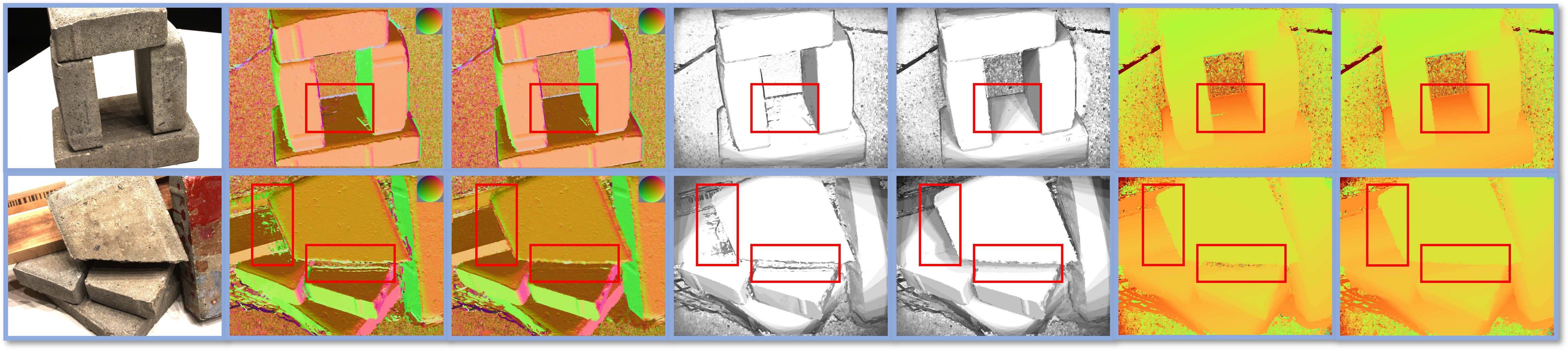
Figure 4: An illustration on the effect of Pixelwise View Selection (PVS). From left to right: input image, normal map without/with PVS, source view set map without/with PVS (brightness indicates the number of views in the source view set), depth map without/with PVS. Challenging areas are marked in red boxes.

5 Artificial Multi-Bee Colony Algorithm

The original Artificial Bee Colony algorithm is a bio-inspired optimization approach proposed by Karaboga [15]. Wang et al. [41] later employ multiple bee colonies to optimize solutions for different pixels and use inter-colony scout bees to facilitate solution propagation.

In MVS context, each solution has four parameters: three for the normal vector and one for the depth value. By representing each solution as a food source, the optimal results are searched by sending out three kinds of bees: employed bees, onlooker bees, and scout bees. The parameterization is conducted in the Euclidean scene space as Gipuma [8] does. Compared to the disparity space, parameterization in scene space avoids the epipolar rectification, and it could generate dense normals in the scene, which could be used for further point cloud fusion [16].

In the Euclidean scene space, the plane equation for 3D object points $\textbf{X}=[X,Y,Z]^{\top}$ would be $\vec{n}^{\top}\textbf{X}=-D$, where $\vec{n}$ is the normal vector and $D$ is the distance to the origin. By placing the reference camera at the origin, the depth $d$ at the pixel $x$ could be inferred with the plane parameters and the camera intrinsic parameters:

$$d=\frac{Df_{x}}{[x-u,f_{x}/f_{y}(y-v),f_{x}]\cdot\vec{n}}$$ (1)

In this equation, $c_{x},c_{y}$ represent the optical center, and $f_{x},f_{y}$ represent the focal length of the camera in pixels which are parameters from camera intrinsic matrix $K$. Under this context, each solution contains four parameters: three for $n$ and one for $d$. Then the pixel $x$ in the reference image $K[I|0]$ is related to the corresponding point $x^{\prime}$ in the source image $K^{\prime}[R|t]$ based on the plane-induced homography [12]:

$$H_{\pi}=K^{\prime}(R-\frac{1}{D}t\vec{n}^{\top})K^{-1}$$ (2)

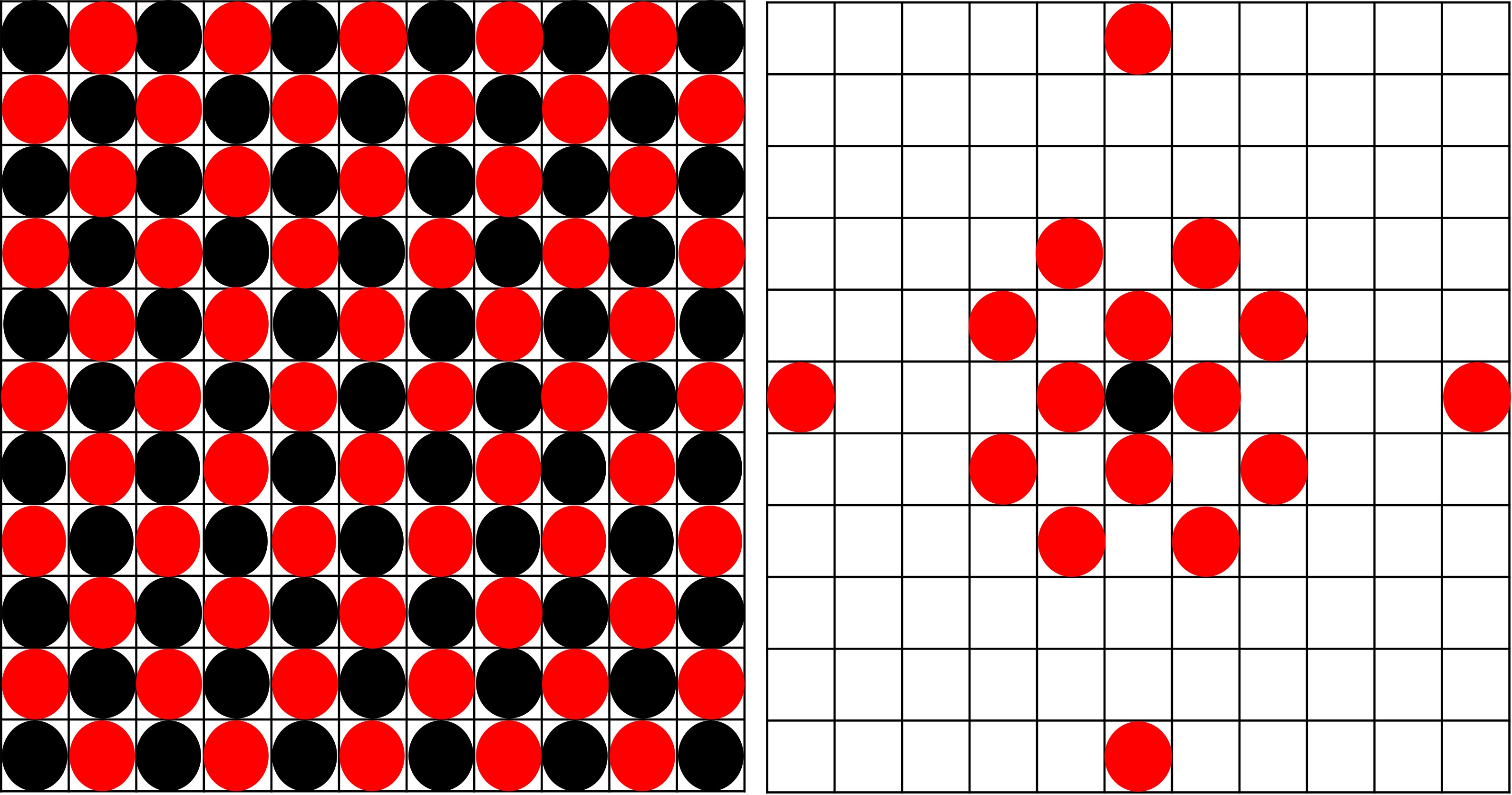
Figure 5: Left: red-black checkerboard pattern. Each block represents a pixel in the image. The pixels in the same color are processed parallelly. Right: the sample space (red) of a center pixel (black).

5.1 Random Initialization

We first randomly generate the same number of hypotheses as preset $\mathit{FoodNumber}$ for each pixel. Each hypothesis contains three parameters for the normal vector $\vec{n}$, and one parameter for plane depth $D$. We follow [23] to uniformly sample the normal vector over the visible hemisphere. Note that since plane depth $D$ is used here, the solutions of pixels on the same plane will have the same set of parameters. Scene depth $d$ could be obtained via equation 1 when needed.

5.2 Matching Cost Evaluation

The similarity between two patches related via plane-induced homography defines whether the hypothesis depicts the scene correctly. In the two-view stereo, the matching cost is straightforward. When extending to multi-view stereo, we adopt the following equation to aggregate the matching cost of hypothesis $\langle d_{i}(x),\vec{n}_{i}(x)\rangle$ in pixel $x$ of the reference image $i$:

$$C(d_{i}(x),\vec{n}_{i}(x))=\begin{dcases}\frac{\sum\limits_{j\in\{S_{src}\}}m(i,j)}{|\{S_{src}\}|-1},&\text{if }|\{S_{src}\}|>1\\ +\infty,&\text{otherwise}\end{dcases}$$ (3)

where $m(i,j)$ represents the matching cost between two patches from reference view $i$ and source view $j$, and $\{S_{src}\}$ is the set of suitable source views for pixel $x$. In this paper, we adopt bilaterally weighted Normalized Cross-Correlation [28] as our matching cost function.

In Equation 3, the aggregation cost is divided by $|\{S_{src}\}|-1$ rather than $|\{S_{src}\}|$ because we expect the results to be an unbiased sample estimate that prefers a larger $\{S_{src}\}$ set. Which is more likely to capture the true normal and depth information than a small set where only several views produce the best results and the rest are invalid (e.g. out of image boundaries).

In addition, we adopt a fitness value to each plane hypothesis:

$$F(d_{i}(x),\vec{n}_{i}(x))=\frac{1}{1+C(d_{i}(x),\vec{n}_{i}(x))}$$ (4)

The fitness for a hypothesis is higher if the aggregation matching cost is lower. The trial count $T(d_{i}(x),\vec{n}_{i}(x))$ is added and set to zero for all food sources in the initialization. It is designed to track whether each food source is updated through iterations.

5.3 Employed Bees

The task for employed bees is to perform a search within the local colonies by randomly perturbing each food source. For each food source, the perturbed food source $y^{\prime}_{x}$ is generated by:

$$y^{\prime}_{x}=y_{x}+R(-1,1)(y_{n}-y_{x})$$ (5)

where $R(-1,1)$ returns a value uniformly distributed between -1 and 1, and $y_{n}$ is another food source randomly selected within the colony. The fitness of the perturbed hypothesis is then evaluated based on the combination of Equation 3 and 4. If the fitness of perturbed food source $F(y^{\prime}_{x})$ is greater than $F(y_{x})$, then $y_{x}$ is replaced by $y^{\prime}_{x}$. Otherwise, set the trial count $T(x)=T(x)+1$.

5.4 Onlooker Bees

The task for onlooker bees is to perform searching in neighboring colonies. Following [8], we adopt a red-black checkerboard pattern for sampling. It divides the image into red and black groups. Pixels in the same color group can be processed in parallel without interfering with others. Figure 5 shows a center pixel’s pattern and sample space.

For every food source $y_{x}$ with a black label, randomly select a colony with a red label following the pattern in Figure 5, and vice versa. Then select the food source $y_{n}$ with the highest fitness value, and evaluate the fitness of the food source $F(y_{n})$ in the current colony. If $F(y_{n})$ is greater than $F(y_{x})$, then $y_{x}$ is replaced by $y_{n}$. Otherwise, set the trial count $T(y_{x})=T(y_{x})+1$.

5.5 Scout Bees

After several iterations after the initialization, the colony’s food sources will converge to a relatively small range. Since employed bees and onlooker bees only perturb or copy the existing solutions, the task for scout bees is to perform global searching and avoid potential local optimum. In this paper, we only want to perform the global searching for $\mathit{FoodNumber}-1$ food sources. The reason is that the food source with the highest fitness value should always be kept in the colony. Therefore, for the rest of the food source, if their trial count $T(y_{x})$ exceeds a preset threshold (it is empirically set to 10), then it is replaced by a randomly generated food source. The idea behind this is that when a food source has not been updated for certain iterations and is not the best in the colony, it may have been stuck in the local optimum. The new food source is evaluated via Equation 4, and the new trial count is set to 0.

6 Geometric Consistency Check

Due to noise and/or deviation from Lambertian property, mismatches sometimes have lower matching costs (or higher fitness scores) than correct matches. To filter out these mismatches, the consistency check is often applied. As shown in Figure 1, our approach alternates between the depth/normal estimation stage and the consistency check stage until the whole process converges. That is, once normal and depth map calculation is completed for all views, the algorithm will cross-check the obtained depth/normal among these views. The solutions that pass the check will be marked as validated for the next calculation cycle. It is worth noting that validated and unvalidated solutions are continued to be refined in future optimizations. Unlike unvalidated solutions, validated ones are used for: 1) enforcing smoothness constraint during intra-image solution propagation; 2) propagating solutions among different views; 3) providing visibility information during future source view selection.

Ideally, if a solution $\langle d_{i}(x),\vec{n}_{i}(x)\rangle$ for pixel $x$ in image $I_{i}$ is correct, it should be consistent with all corresponding solutions in the source views used for pixel $x$. That is, after applying homography transform $H^{ij}$ between view $I_{i}$ and one of the source view $I_{j}$ for pixel $x$, we should have $H^{ij}(d_{i}(x))=d_{j}(H^{ij}(x))$ and $H^{ij}(\vec{n}_{i}(x))=\vec{n}_{j}(H^{ij}(x))$. In practice, we consider solution $\langle d_{i}(x),\vec{n}_{i}(x)\rangle$ is consistent with source view $I_{j}$ if the following two criteria hold:

$$|H^{ij}(d_{i}(x))-d_{j}(H^{ij}(x))| < {\mathit{T}}_{depth},$$ (6)

$$\arccos(H^{ij}(\vec{n}_{i}(x))\cdot\vec{n}_{j}(H^{ij}(x))) < {\mathit{T}}_{normal}$$

where ${\mathit{T}}_{depth}$ and ${\mathit{T}}_{normal}$ are two preset thresholds (it is set to 0.01 mm and 30 degrees in practice). In addition, instead of requiring all source views used for pixel $x$ to be consistent with $\langle d_{i}(x),\vec{n}_{i}(x)\rangle$, we relax the constraint by allowing a small percentage of these views do not satisfy the above conditions. That is, $\langle d_{i}(x),\vec{n}_{i}(x)\rangle$ is labeled as verified if it is consistent with 70% or more of the source views $\{I_{src}\}$ selected for pixel $x$.

6.1 Propagation Between Views

Initially, solution propagation only appears in neighboring colonies within the same image (referred as intra-image propagation) via onlooker bees. It is one of the vital concepts in PatchMatch-based multi-view stereo. In this paper, we propose inter-image propagation as well, which enables the solution to propagate between pixels in different images related by consistency check. Figure 6 shows an example of propagation between views. The key concept is to propagate each solution that is consistent with at least one other source view to views that do not have validated solutions at the corresponding locations. This helps to speed up the convergence and prevent potential local optimum.

6.2 Smoothness Constraint

Not being able to handle textureless areas properly is a significant limitation for the PatchMatch-based methods [27]. In binocular stereo, this problem is often addressed by introducing an additional smoothness term, which converts per-pixel optimization into global optimization. Solving global optimization under the MVS setting can be highly computationally expensive. Hence, we applied a simple yet effective approach, which adds fitness reward to solutions propagated by onlooker bees. The key observation is that the fitness values for the correct match and mismatches are similar in textureless areas. Adding a small reward to the validated solutions propagated by onlooker bees effectively encourages the same fitting plane being selected at the current solution. The smoothness is therefore enforced, and flat textureless surfaces can be properly modeled. For areas with distinct textures, the small reward will not affect the search for optimal solutions.

7 Fusion

Follows [8, 28], after obtaining all the depth and normal maps, we fuse them into a single point cloud. More specifically, for $N$ images in the scene, we consequently select each image as the reference image and convert its depth map to 3D points in the world coordinate, then project them to the rest $N-1$ views. If the relative depth difference is less than 0.01 mm, and the angle between normals is smaller than 30 degrees, then it is counted as a consistent view. If there exist more than three consistent views, then the point will be accepted in the result. Finally, the points that are related by the depth and normal estimates are averaged into a 3D point in the result point cloud.

Method	Acc.(mm)	Comp.(mm)	Overall
Furukawa [7]	0.605	0.842	0.724
Tola [38]	0.307	1.097	0.702
COLMAP [28]	0.400	0.532	0.664
Campbell [4]	0.753	0.540	0.647
Gipuma [8]	0.273	0.687	0.480
Ours	0.385	0.388	0.386

Table 1: Quantitative results for non-learning-based approaches on full DTU dataset. Lower is better. Our method ranks first in terms of Completeness and Overall metrics.

Method	Acc.(mm)	Comp.(mm)	Overall
Non-Learning-based
Furukawa [7]	0.613	0.941	0.777
Tola [38]	0.342	1.190	0.766
Campbell [4]	0.835	0.554	0.695
Gipuma [8]	0.283	0.873	0.578
COLMAP [28]	0.411	0.657	0.534
Ours	0.405	0.381	0.393
Learning-based
SurfaceNet [13]	0.450	1.040	0.745
MVSNet [47]	0.396	0.527	0.462
P-MVSNet [21]	0.406	0.434	0.420
R-MVSNet [48]	0.383	0.452	0.417
CasMVSNet [10]	0.325	0.385	0.355
PatchMatchNet [39]	0.427	0.277	0.352
UniMVSNet [26]	0.352	0.278	0.315

Table 2: Quantitative results on DTU evaluation set. Both learning-based and non-learning-based approaches are listed for impartial comparison.

8 Experiments

We evaluate our method on the DTU Robot Image dataset [1]. In this section, we present the dataset details, evaluation results, ablation study for key components, and implementation details. Noted that $\mathit{FoodNum}$ is set to 10 in our experiments.

8.1 DTU Robot Image Dataset

As our main testing dataset, the DTU dataset contains 124 different scenes captured by a structured light scanner mounted on an industrial robot arm. Each scene has been taken from 49 or 64 positions with seven different lighting conditions. In this paper, we select the most diffuse set. The image resolution is $1600\times 1200$, and the camera calibration parameters are provided.

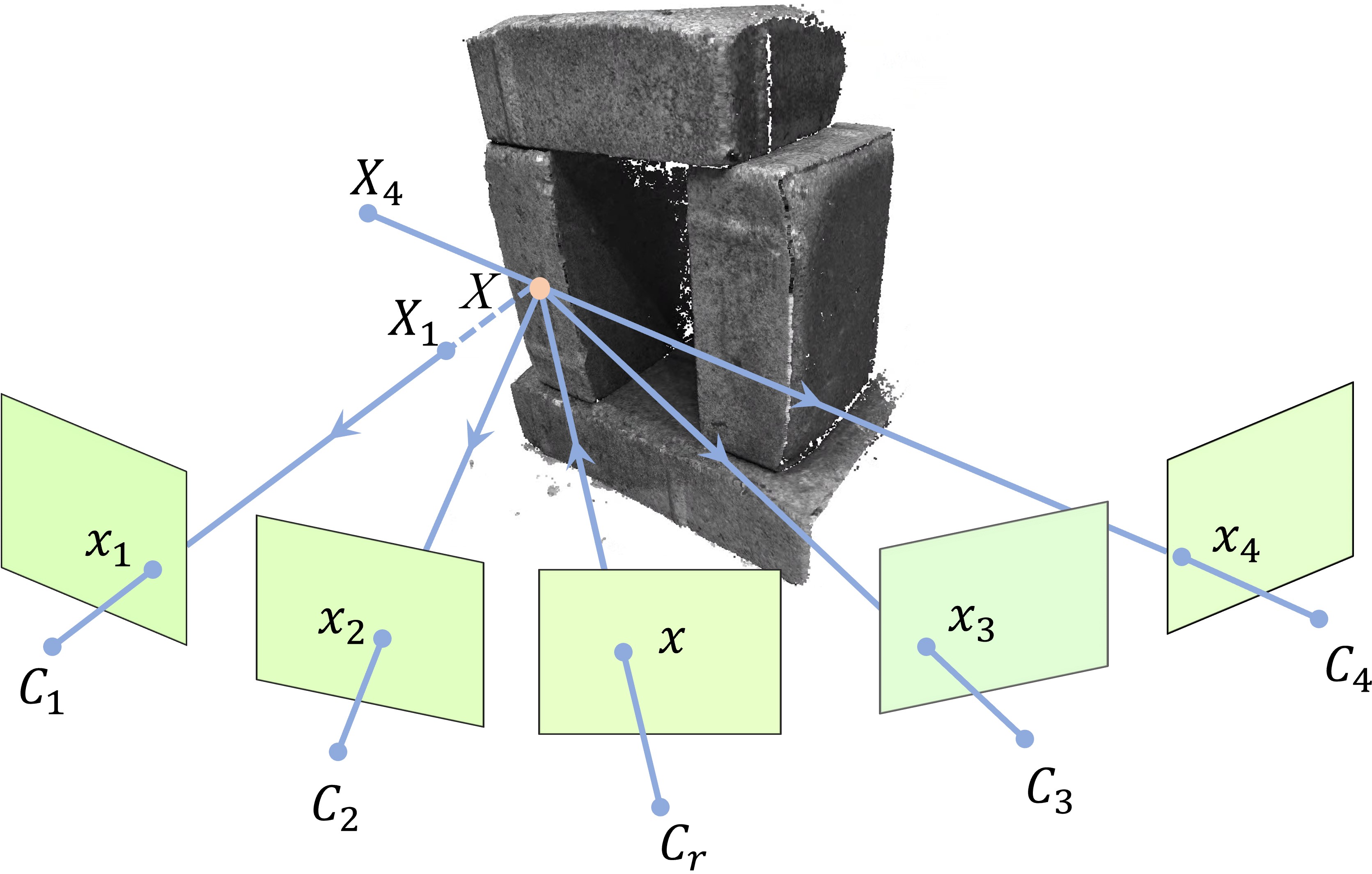
Figure 6: Illustration of the Propagation Between Views. The solution in reference view $C_{r}$ is consistent with two of its neighboring views: $C_{2},C_{3}$. While the rest of the two are not consistent with $C_{r}$. Then the solution will be propagated to $x_{1},x_{4}$ to check whether it is a better solution to replace existing ones.

Figure 7: Visualization results of the proposed method in scene 11, 95 and 100 in DTU dataset. From left to right: Tola [38], Furukawa [7], Campbell [4], point cloud without Smoothness Constraint, point cloud with Smoothness Constraint, ground truth.

Figure 8: Illustration on the effect of the Smoothness Constraint (SC) and Pixelwise View Selection (PVS). From top to bottom: scene 19, 59, 100 from the DTU dataset. From left to right: input image, normal map without SC & PVS, normal map with SC, normal map with SC & PVS, depth map without SC & PVS, depth map with SC, depth map with SC & PVS. Challenging areas are marked in red boxes.

8.2 Point Cloud Evaluation

Accuracy is measured as the distance from the reconstruction point cloud to the structured light reference. Completeness is measured from the structured light reference to the reconstruction point cloud. The overall score is computed by averaging the accuracy and completeness. Note that the reconstruction point cloud is downsampled to ensure unbiased evaluation since strongly textured regions generally have dense 3D points. The evaluation program is provided by the authors.

For this dataset, we present two versions of quantitative results: one for comparison of the non-learning-based methods and the other for comparison of both the learning-based and non-learning-based methods. For non-learning-based method evaluation, we follow the protocol specified by the authors of the dataset by testing 80 different scenes. For Learning-based method evaluation, we follow [47] by using the validation set containing 22 different scenes for impartial comparison. In Table 1, we present the quantitative results for non-learning-based approaches on the full DTU dataset. Our approach performs the best in both completeness and overall metrics. In Table 2, we present the quantitative results for both learning-based and non-learning-based methods on the DTU evaluation set. Our method shows competitive performance to the learning-based methods.

8.3 Ablation Study

We here present the ablation study of the proposed method. The baseline method is generated using AMBC with all three types of bees: employed bees, onlooker bees, and scout bees. Our proposed baseline method with smoothness constraint, pixelwise view selection, and propagation between views shows the best performance. Note that propagation between views only speeds up the convergence because it does not modify the solution space. Therefore it does not have a significant impact on result accuracy.

Figure 4 demonstrates the effect of the pixelwise view selection in occluded regions. The pixel-wise view selection could handle the occluded regions and generate correct normal and depth estimation. Figure 7 shows a comparison of the point clouds on scene 11, 95, and 100 in the DTU dataset. The proposed method with smoothness constraint clearly outperforms in low-textured areas. In addition, only a few noisy/incorrect points are introduced along the edges of the surfaces. Figure 8 illustrates the effect of the combination of smoothness constraint and pixelwise view selection. The best results are obtained by applying both of them. The numerical results of the ablation study are provided in Supplementary Materials.

9 Conclusion

In this paper, we present a visibility-aware pixelwise view selection method for PatchMatch-based multi-view stereo. View selection is progressively improved for individual pixels as more knowledge of scene geometry is obtained. Selected views are used for both matching cost evaluation and consistency check. When applying Artificial Multi-Bee Colony (AMBC) to search optimal solutions for different pixels in parallel, between-colony onlooker bees are used for intra-image and inter-image solution propagation. To tackle the lack of photometric cues at low-textured regions, fitness rewards are introduced on those solutions verified by consistency check. Experiments on the DTU dataset demonstrate that our method achieves state-of-the-art performance among the non-learning-based methods. Ablation study shows that our two main components, visibility-aware pixelwise view selection, and smoothness rewards, can notably improve the handling of occluded and low-textured areas. The source code will be released after the acceptance of the paper.

References

- [1] Henrik Aanæs, Rasmus Ramsbøl Jensen, George Vogiatzis, Engin Tola, and Anders Bjorholm Dahl. Large-scale data for multiple-view stereopsis. International Journal of Computer Vision, pages 1–16, 2016.
- [2] Connelly Barnes, Eli Shechtman, Adam Finkelstein, and Dan B Goldman. Patchmatch: A randomized correspondence algorithm for structural image editing. ACM Trans. Graph., 28(3):24, 2009.
- [3] Michael Bleyer, Christoph Rhemann, and Carsten Rother. Patchmatch stereo-stereo matching with slanted support windows. In The British Machine Vision Conference (BMVC), volume 11, pages 1–11, 2011.
- [4] Neill DF Campbell, George Vogiatzis, Carlos Hernández, and Roberto Cipolla. Using multiple hypotheses to improve depth-maps for multi-view stereo. In European Conference on Computer Vision, pages 766–779. Springer, 2008.
- [5] Zhiqin Chen and Hao Zhang. Learning implicit fields for generative shape modeling. In Proceedings of the IEEE/CVF Conference on Computer Vision and Pattern Recognition, pages 5939–5948, 2019.
- [6] Christopher B Choy, Danfei Xu, JunYoung Gwak, Kevin Chen, and Silvio Savarese. 3d-r2n2: A unified approach for single and multi-view 3d object reconstruction. In European Conference on Computer Vision, pages 628–644. Springer, 2016.
- [7] Yasutaka Furukawa and Jean Ponce. Accurate, dense, and robust multiview stereopsis. IEEE Transactions on Pattern Analysis and Machine Intelligence, 32(8):1362–1376, 2009.
- [8] Silvano Galliani, Katrin Lasinger, and Konrad Schindler. Massively parallel multiview stereopsis by surface normal diffusion. In Proceedings of the IEEE International Conference on Computer Vision, pages 873–881, 2015.
- [9] Clément Godard, Oisin Mac Aodha, and Gabriel J Brostow. Unsupervised monocular depth estimation with left-right consistency. In Proceedings of the IEEE Conference on Computer Vision and Pattern Recognition, pages 270–279, 2017.
- [10] Xiaodong Gu, Zhiwen Fan, Siyu Zhu, Zuozhuo Dai, Feitong Tan, and Ping Tan. Cascade cost volume for high-resolution multi-view stereo and stereo matching. In Proceedings of the IEEE/CVF Conference on Computer Vision and Pattern Recognition, pages 2495–2504, 2020.
- [11] Emrah Hancer, Bing Xue, Dervis Karaboga, and Mengjie Zhang. A binary abc algorithm based on advanced similarity scheme for feature selection. Applied Soft Computing, 36:334–348, 2015.
- [12] Richard Hartley and Andrew Zisserman. Multiple view geometry in computer vision. Cambridge university press, 2003.
- [13] Mengqi Ji, Juergen Gall, Haitian Zheng, Yebin Liu, and Lu Fang. Surfacenet: An end-to-end 3d neural network for multiview stereopsis. In Proceedings of the IEEE International Conference on Computer Vision, pages 2307–2315, 2017.
- [14] Dervis Karaboga and Bahriye Basturk. Artificial bee colony (abc) optimization algorithm for solving constrained optimization problems. In International Fuzzy Systems Association World Congress, pages 789–798. Springer, 2007.
- [15] Dervis Karaboga et al. An idea based on honey bee swarm for numerical optimization. Technical report, Technical Report-tr06, Erciyes University, Engineering Faculty, Computer …, 2005.
- [16] Michael Kazhdan and Hugues Hoppe. Screened poisson surface reconstruction. ACM Transactions on Graphics (ToG), 32(3):1–13, 2013.
- [17] Arno Knapitsch, Jaesik Park, Qian-Yi Zhou, and Vladlen Koltun. Tanks and temples: Benchmarking large-scale scene reconstruction. ACM Transactions on Graphics (ToG), 36(4):1–13, 2017.
- [18] Kiriakos N Kutulakos and Steven M Seitz. A theory of shape by space carving. International Journal of Computer Vision, 38(3):199–218, 2000.
- [19] Maxime Lhuillier and Long Quan. A quasi-dense approach to surface reconstruction from uncalibrated images. IEEE Transactions on Pattern Analysis and Machine Intelligence, 27(3):418–433, 2005.
- [20] Fayao Liu, Chunhua Shen, Guosheng Lin, and Ian Reid. Learning depth from single monocular images using deep convolutional neural fields. IEEE Transactions on Pattern Analysis and Machine Intelligence, 38(10):2024–2039, 2015.
- [21] Keyang Luo, Tao Guan, Lili Ju, Haipeng Huang, and Yawei Luo. P-mvsnet: Learning patch-wise matching confidence aggregation for multi-view stereo. In Proceedings of the IEEE/CVF International Conference on Computer Vision, pages 10452–10461, 2019.
- [22] Wendong Mao, Mingjie Wang, Hui Huang, and Minglun Gong. A robust framework for multi-view stereopsis. The Visual Computer, 38(5):1539–1551, 2022.
- [23] George Marsaglia. Choosing a point from the surface of a sphere. The Annals of Mathematical Statistics, 43(2):645–646, 1972.
- [24] Lars Mescheder, Michael Oechsle, Michael Niemeyer, Sebastian Nowozin, and Andreas Geiger. Occupancy networks: Learning 3d reconstruction in function space. In Proceedings of the IEEE/CVF Conference on Computer Vision and Pattern Recognition, pages 4460–4470, 2019.
- [25] Michael Niemeyer, Lars Mescheder, Michael Oechsle, and Andreas Geiger. Differentiable volumetric rendering: Learning implicit 3d representations without 3d supervision. In Proceedings of the IEEE/CVF Conference on Computer Vision and Pattern Recognition, pages 3504–3515, 2020.
- [26] Rui Peng, Rongjie Wang, Zhenyu Wang, Yawen Lai, and Ronggang Wang. Rethinking depth estimation for multi-view stereo: A unified representation. In Proceedings of the IEEE/CVF Conference on Computer Vision and Pattern Recognition, pages 8645–8654, 2022.
- [27] Andrea Romanoni and Matteo Matteucci. Tapa-mvs: Textureless-aware patchmatch multi-view stereo. In Proceedings of the IEEE/CVF International Conference on Computer Vision, pages 10413–10422, 2019.
- [28] Johannes L Schönberger, Enliang Zheng, Jan-Michael Frahm, and Marc Pollefeys. Pixelwise view selection for unstructured multi-view stereo. In European Conference on Computer Vision, pages 501–518. Springer, 2016.
- [29] Steven M Seitz, Brian Curless, James Diebel, Daniel Scharstein, and Richard Szeliski. A comparison and evaluation of multi-view stereo reconstruction algorithms. In 2006 IEEE Computer Society Conference on Computer Vision and Pattern Recognition (CVPR’06), volume 1, pages 519–528. IEEE, 2006.
- [30] Steven M Seitz and Charles R Dyer. Photorealistic scene reconstruction by voxel coloring. International Journal of Computer Vision, 35(2):151–173, 1999.
- [31] Sudipta N Sinha, Philippos Mordohai, and Marc Pollefeys. Multi-view stereo via graph cuts on the dual of an adaptive tetrahedral mesh. In 2007 IEEE 11th International Conference on Computer Vision, pages 1–8. IEEE, 2007.
- [32] Vincent Sitzmann, Eric Chan, Richard Tucker, Noah Snavely, and Gordon Wetzstein. Metasdf: Meta-learning signed distance functions. Advances in Neural Information Processing Systems, 33:10136–10147, 2020.
- [33] Qiuhang Tan, Hejun Wu, Biao Hu, and Xingcheng Liu. An improved artificial bee colony algorithm for clustering. In Proceedings of the Companion Publication of the 2014 Annual Conference on Genetic and Evolutionary Computation, pages 19–20, 2014.
- [34] Jiapeng Tang, Xiaoguang Han, Junyi Pan, Kui Jia, and Xin Tong. A skeleton-bridged deep learning approach for generating meshes of complex topologies from single rgb images. In Proceedings of the IEEE/CVF Conference on Computer Vision and Pattern Recognition, pages 4541–4550, 2019.
- [35] Jiapeng Tang, Xiaoguang Han, Mingkui Tan, Xin Tong, and Kui Jia. Skeletonnet: A topology-preserving solution for learning mesh reconstruction of object surfaces from rgb images. IEEE Transactions on Pattern Analysis and Machine Intelligence, 2021.
- [36] Maxim Tatarchenko, Alexey Dosovitskiy, and Thomas Brox. Octree generating networks: Efficient convolutional architectures for high-resolution 3d outputs. In Proceedings of the IEEE International Conference on Computer Vision, pages 2088–2096, 2017.
- [37] Hugues Thomas, Charles R Qi, Jean-Emmanuel Deschaud, Beatriz Marcotegui, François Goulette, and Leonidas J Guibas. Kpconv: Flexible and deformable convolution for point clouds. In Proceedings of the IEEE/CVF International Conference on Computer Vision, pages 6411–6420, 2019.
- [38] Engin Tola, Vincent Lepetit, and Pascal Fua. Daisy: An efficient dense descriptor applied to wide-baseline stereo. IEEE Transactions on Pattern Analysis and Machine Intelligence, 32(5):815–830, 2009.
- [39] Fangjinhua Wang, Silvano Galliani, Christoph Vogel, Pablo Speciale, and Marc Pollefeys. Patchmatchnet: Learned multi-view patchmatch stereo. In Proceedings of the IEEE/CVF Conference on Computer Vision and Pattern Recognition, pages 14194–14203, 2021.
- [40] Xiang Wang, Chen Wang, Bing Liu, Xiaoqing Zhou, Liang Zhang, Jin Zheng, and Xiao Bai. Multi-view stereo in the deep learning era: A comprehensive review. Displays, 70:102102, 2021.
- [41] Yunhai Wang, Yiming Qian, Yang Li, Minglun Gong, and Wolfgang Banzhaf. Artificial multi-bee-colony algorithm for k-nearest-neighbor fields search. In Proceedings of the Genetic and Evolutionary Computation Conference 2016, pages 1037–1044, 2016.
- [42] Yi Wei, Shaohui Liu, Yongming Rao, Wang Zhao, Jiwen Lu, and Jie Zhou. Nerfingmvs: Guided optimization of neural radiance fields for indoor multi-view stereo. In Proceedings of the IEEE/CVF International Conference on Computer Vision, pages 5610–5619, 2021.
- [43] Shihao Wu, Peter Bertholet, Hui Huang, Daniel Cohen-Or, Minglun Gong, and Matthias Zwicker. Structure-aware data consolidation. IEEE Transactions on Pattern Analysis and Machine Intelligence, 40(10):2529–2537, 2017.
- [44] Qingshan Xu and Wenbing Tao. Multi-scale geometric consistency guided multi-view stereo. In Proceedings of the IEEE/CVF Conference on Computer Vision and Pattern Recognition, pages 5483–5492, 2019.
- [45] Qingshan Xu and Wenbing Tao. Planar prior assisted patchmatch multi-view stereo. In Proceedings of the AAAI Conference on Artificial Intelligence, volume 34, pages 12516–12523, 2020.
- [46] Guandao Yang, Xun Huang, Zekun Hao, Ming-Yu Liu, Serge Belongie, and Bharath Hariharan. Pointflow: 3d point cloud generation with continuous normalizing flows. In Proceedings of the IEEE/CVF International Conference on Computer Vision, pages 4541–4550, 2019.
- [47] Yao Yao, Zixin Luo, Shiwei Li, Tian Fang, and Long Quan. Mvsnet: Depth inference for unstructured multi-view stereo. In Proceedings of the European Conference on Computer Vision (ECCV), pages 767–783, 2018.
- [48] Yao Yao, Zixin Luo, Shiwei Li, Tianwei Shen, Tian Fang, and Long Quan. Recurrent mvsnet for high-resolution multi-view stereo depth inference. In Proceedings of the IEEE/CVF Conference on Computer Vision and Pattern Recognition, pages 5525–5534, 2019.
- [49] Yao Yao, Zixin Luo, Shiwei Li, Jingyang Zhang, Yufan Ren, Lei Zhou, Tian Fang, and Long Quan. Blendedmvs: A large-scale dataset for generalized multi-view stereo networks. In Proceedings of the IEEE/CVF Conference on Computer Vision and Pattern Recognition, pages 1790–1799, 2020.
- [50] Zhichao Yin and Jianping Shi. Geonet: Unsupervised learning of dense depth, optical flow and camera pose. In Proceedings of the IEEE Conference on Computer Vision and Pattern Recognition, pages 1983–1992, 2018.
- [51] Guopu Zhu and Sam Kwong. Gbest-guided artificial bee colony algorithm for numerical function optimization. Applied Mathematics and Computation, 217(7):3166–3173, 2010.