Joint Probability Trees

Abstract

We introduce Joint Probability Trees (JPT), a novel approach that makes learning of and reasoning about joint probability distributions tractable for practical applications. JPTs support both symbolic and subsymbolic variables in a single hybrid model, and they do not rely on prior knowledge about variable dependencies or families of distributions. JPT representations build on tree structures that partition the problem space into relevant subregions that are elicited from the training data instead of postulating a rigid dependency model prior to learning. Learning and reasoning scale linearly in JPTs, and the tree structure allows white-box reasoning about any posterior probability $P(Q|E)$, such that interpretable explanations can be provided for any inference result. Our experiments showcase the practical applicability of JPTs in high-dimensional heterogeneous probability spaces with millions of training samples, making it a promising alternative to classic probabilistic graphical models.

in not Null &and or yield each

1 Introduction

Joint probability distributions offer a wide range of high-potential applications in engineering, science, and technology (Chater et al., 2006; Griffiths et al., 2008; Knill & Pouget, 2004). Besides families of continuous distributions, probabilistic graphical models (PGMs), such as Bayesian networks and Markov random fields (Koller & Friedman, 2009), are the de-facto standard in probabilistic knowledge representation. They provide graph-based languages to model dependencies and independencies of variables, and local joint or conditional distributions that quantify the statistical dependencies. However, the practical applicability of PGMs suffers from the representational and computational complexity of learning and reasoning. Exponential runtime for learning and reasoning often can only be avoided by introducing strong independence assumptions that must be known prior to learning and may turn out to be too great simplifications of a model to be of practical use (Besag, 1975; Jain, 2012). As a simple example, consider a probability space $\langle X,Y,C\rangle$ of two numeric variables, $X$ and $Y$, and one symbolic variable $C$, $\textit{dom}(C)=\{\textit{Red},\textit{Blue}\}$ as illustrated in Figures 1(a) and 1(b). Let the symbolic values Red and Blue demaracate two clusters that are approximately normally distributed. Classic methods for density estimation postulate a mathematical model and apply the maximum likelihood and expectation/maximization principles in order to find the model parameters that fit the data best. However, this learning process is expensive since the unconstrained parameter space is huge and most learning methods do not exploit the structure of the training data and their underlying distribution.

(a) The ground truth distribution

(b) Scatterplot of the sample data

(c) The marginal $P(X,Y)$
represented by the JPT in (d)

(d) The tree structure of the corresponding JPT

Figure 1: Example of a joint probability distribution of two numeric variables $(X,Y)$ and one symbolic variable (color). Enlarged versions of the figures can be found in the supplementary material.

In this paper, we introduce Joint Probability Trees (JPT), a novel approach to represent, learn, and reason about uncertain knowlegde acquired from data. JPTs are model-free shallow deterministic probabilistic circuits and they exploit the structure of the data to be learnt from in a greedy fashion in order to construct a tree structure that partitions the problem space recursively into subspaces. In its leaves, marginal distributions, represented by cumulative distribution functions (CDFs) over all variables in the respective subspace are maintained, which can be superimposed in order to obtain a sound and globally consistent posterior belief. As opposed to most PGMs, dependencies among variables in JPTs do not need to be known at design time and only very mild assumptions about models are required. Figure 1(d) shows such a tree structure that has been learnt from the data in Figure 1(b), and the marginal distribution in Figure 1(c) shows indeed close resemblance to the ground truth distribution in Figure 1(a). JPTs allow the computation of any posterior distribution in a transparent and explainable way, such that the rationale for any inference result can be provided in a human-interpretable form.

The contributions of this paper are the following. First, we formally introduce the concept of Joint Probability Trees as a novel framework for knowledge representation and reasoning in probabilistic hybrid domains and we present algorithms for the learning of and reasoning about JPTs. Second, we adapt the concept of quantile-parameterized distributions for the efficient learning of univariate continuous distributions without prior assumptions about their functional forms, and third, we investigate and showcase the performance of JPTs empirically on publicly available datasets.

2 Joint Probability Trees

In this section, we introduce the concept of Joint Probability Trees (JPTs) more formally. Let us denote the $D$-dimensional problem space under consideration as $X=\langle X_{1},\ldots,X_{D}\rangle$, where $X$ is a vector of random variables $X_{i}$, whose domains we denote by $\textit{dom}(X_{i})$. The set of possible worlds, i.e. all possible complete variable assignments, is denoted by $\mathcal{X}$, and a specific assignment to all variables in $X$, by $x=\langle x_{1},\ldots,x_{D}\rangle$, where $x\in\mathcal{X}$. As a representational formalism, JPTs make use of tree-like structures like classification and regression trees (Breiman et al., 2017b). Trees have a couple of desirable properties that put themselves forward to be used as a knowledge representation formalism. Most notably, they (1) are simple to understand and interpret, (2) can be thought of as white box models that foster explainable decision making, (3) are compact and sparse representations that allow efficient learning and reasoning. These features are leveraged through the model structures implementing a recursive partition of the problem space under consideration. Let $T:\mathcal{X}\mapsto\Lambda$ be a tree-like structure that associates an input sample $x\in\mathcal{X}$ with one of its leaves $\Lambda=\{\lambda_{1},\ldots,\lambda_{N}\}$. The recursive partitioning through a tree structure guarantees that $T$ is exhaustive and mutually exclusive.

As a consequence, the result of the application of $T$, $T(x)$, can be treated as a random variable that indicates which leaf $\lambda$ an arbitrary sample $x$ will be associated with. We thus introduce an auxiliary variable $L$, $\textit{dom}(L)=\Lambda$, that extends the problem space $X$ by $L$ and hence forms a new probability space $X^{\prime}=\left\langle X,L\right\rangle$. Applying the law of total probability, we can marginalize the prior probabilities of $X$ over $X^{\prime}$ by

$$P(X=x)=\sum_{\lambda\in\Lambda}P\!\left(\!\begin{array}[]{c|c}\begin{array}[]{c}X\end{array}&\begin{array}[]{c}L=\lambda\end{array}\end{array}\!\right)P\!\left(L=\lambda\right).$$ (4)

The leaf priors $P\!\left(L=\lambda\right)$ can be easily obtained from the portions of training data that are covered by the respective leaf during training and can be permanently stored in the leaf data structure. The leaf-conditional distributions $P\!\left(\!\begin{array}[]{c|c}\begin{array}[]{c}X_{1},\ldots,X_{D}\end{array}&\begin{array}[]{c}L=\lambda\end{array}\end{array}\!\right)$, however, are more difficult to represent as they still comprise the joint distributions over $X$. Here, we introduce the naïve Bayes assumption that postulates conditional independence among all $X_{i}$, once $L$ is known. This assumption is reasonable as the leaves in $T$ represent contiguous subregions in $\mathcal{X}$ that are formed during learning by minimizing the mutual information of variables (or maximizing information gain, respectively), which can be proven equivalent to statistical dependence (Murphy, 2022). Assuming independence of variables in the leaf nodes in turn allows to represent the priors over $X_{i}$ conditioned by the respective subspace in every leaf node of $T$ in an extremely compact way:

$$P(X=x)=\sum_{\lambda\in\Lambda}P\!\left(L=\lambda\right)\prod_{i}P\!\left(\!\begin{array}[]{c|c}\begin{array}[]{c}X_{i}=x_{i}\end{array}&\begin{array}[]{c}L=\lambda\end{array}\end{array}\!\right).$$ (8)

We call (8) the JPT distribution, which can be used in order to compute the marginal probability of a possible world $x\in\mathcal{X}$. It can be regarded as a mixture model, whose mixing coefficients are represented by the leaf priors, and the local distributions are given by the priors in the respective leaves.

2.1 Reasoning in Joint Probability Trees

Computing the marginalization over the tree leaves in (8) may seem like unnecessary effort as, once $x$ is known, $\lambda$ is fully determined by $T$. However, mixing the leaf distributions becomes inevitable if the values of only a fraction of variables $E\subset X$ are known in advance and the posterior probability of a subset $Q\subseteq X$, $P\!\left(\!\begin{array}[]{c|c}\begin{array}[]{c}Q\end{array}&\begin{array}[]{c}E\end{array}\end{array}\!\right)$, needs to be computed. Extending (8) to canonical posterior inference can be achieved in a straightforward way by introducing background evidence to the JPT distribution:

$$P\!\left(\!\begin{array}[]{c|c}\begin{array}[]{c}q\end{array}&\begin{array}[]{c}e\end{array}\end{array}\!\right)=\sum_{\lambda\in\Lambda}P\!\left(\!\begin{array}[]{c|c}\begin{array}[]{c}\lambda\end{array}&\begin{array}[]{c}e\end{array}\end{array}\!\right)\prod_{i}P\!\left(\!\begin{array}[]{c|c}\begin{array}[]{c}q_{i}\end{array}&\begin{array}[]{c}\lambda,e_{i}\end{array}\end{array}\!\right),$$ (18)

where $q=\langle q_{1},\ldots,q_{D}\rangle$ is a vector of values of the query variables and $e=\langle e_{1},\ldots,e_{D}\rangle$ is a vector of constraints $e_{i}$ for the variables $X_{i}$. Note that, because of the naïve Bayes assumption, $q_{i}$ only depends on the constraints on the respective same variable $X_{i}$, i.e. $e_{i}$, instead of the entire vector $e$. The most interesting part of the posterior in (18) is the factor $P\!\left(\!\begin{array}[]{c|c}\begin{array}[]{c}\lambda\end{array}&\begin{array}[]{c}e\end{array}\end{array}\!\right)$, the probability that a sample satisfying the constraints $e$ will be associated with leaf $\lambda$. While the pure leaf priors $P\!\left(\lambda\right)$ can be obtained from their associated data portions, the conditional $P\!\left(\!\begin{array}[]{c|c}\begin{array}[]{c}\lambda\end{array}&\begin{array}[]{c}e\end{array}\end{array}\!\right)$ is slightly more complex to compute. However, the tree structure of $T$ can be exploited as an efficient approximation as follows. According to Bayes’ theorem, $P\!\left(\!\begin{array}[]{c|c}\begin{array}[]{c}\lambda\end{array}&\begin{array}[]{c}e\end{array}\end{array}\!\right)\propto P\!\left(\!\begin{array}[]{c|c}\begin{array}[]{c}e\end{array}&\begin{array}[]{c}\lambda\end{array}\end{array}\!\right)\cdot P\!\left(\lambda\right)$ holds. We can thus compute the distribution $P\!\left(\!\begin{array}[]{c|c}\begin{array}[]{c}L\end{array}&\begin{array}[]{c}e\end{array}\end{array}\!\right)$ by evaluating $P\!\left(\!\begin{array}[]{c|c}\begin{array}[]{c}e\end{array}&\begin{array}[]{c}\lambda\end{array}\end{array}\!\right)\cdot P\!\left(\lambda\right)$ for every $\lambda$ and normalizing the results to form a proper distribution. $P\!\left(\!\begin{array}[]{c|c}\begin{array}[]{c}e\end{array}&\begin{array}[]{c}\lambda\end{array}\end{array}\!\right)$ can in turn be factorized according to $\prod_{i}P\!\left(\!\begin{array}[]{c|c}\begin{array}[]{c}e_{i}\end{array}&\begin{array}[]{c}\lambda\end{array}\end{array}\!\right)$ due to the conditional independence assumption, which corresponds to the prior distributions stored in every leaf of $T$. A significant performance gain can be achieved by testing both $q$ and $e$ against the path conditions of every leaf $\lambda$. If either of the two violates a path condition, the entire subtree can be pruned for a specific reasoning problem.

2.2 Learning of Joint Probability Trees

In order to learn a JPT from data, we propose a variant of the popular and well-known tree learning methods, which we introduce in this section. C4.5 (Quinlan, 1993) and CART (Breiman et al., 1984) are very successful variants of induction algorithms for classification and regression trees. Essentially, a tree is being built by splitting the input data into subsets constituting the input data for the successor children. The splitting consists of a variable or a variable/value pair that marks a pivot position in the observable feature space optimizing some criterion of impurity with respect to the split data sets. The split constitutes the root node of the tree and the process is repeated on each of the child subsets recursively and terminates when the impurity with respect to the target variables within a subset at a node is minimal or when splitting no longer reduces the impurity. The result of the procedure is a tree structure $T$, whose inner nodes represent decision nodes at which a single input vector $x$ is evaluated according to the pivot variable attached to the respective node and the subsequent child node to proceed with is determined by the value of that variable. If the child node does not have any further children, a terminal node is reached in which the predictive values of the target variables are stored, which constitutes the return value $T(x)$ of the tree. For a more detailed discussion of tree learning we refer to (Loh, 2014).

Generative learning

Ordinary classification and regression tree learning is defined over dedicated feature (input) and target (output) variables of the problem space and therefore it is also called a discriminative learning setting. In each node, the best possible split of the remaining data is looked for in the set of feature variables and their domains, and every possible split is evaluated with respect to its potential to reduce the impurity of the target variables. Although discriminative learning of JPTs is also possible, we focus here on the generative learning case. In contrast to discriminative CART learning, in JPTs, the entire set of variables $X$ functions both as feature and as target variables. This means that in every decision node during the learning process, the node impurity is evaluated with respect to all available variables $X_{i}$, and all variables $X_{i}$ are considered as potential split candidates.

As JPTs support both symbolic and numeric variables, a measure of impurity is needed to account for this hybrid character of the model. Here, the difficulty arises that typical error measures for numerical data, e.g. the mean squared error (MSE) and impurity measures for symbolic data, e.g. entropy, reside in different and incompatible value ranges. In order to harmonize the two worlds of symbolic and subsymbolic impurity, we propose a combined measure of normalized, relative impurity improvement as follows. For a distribution over a symbolic random variable $X$, its entropy is defined by $H(P(X))=-\sum_{x\in\textit{dom}(X)}P(x)\log P(x)$. In CART learning, a possible split is considered better the more it reduces the expected entropy over the children induced by the split. As a multinomial variable has its highest entropy in the uniform distribution, we can normalize the entropy with respect to the maximal entropy a distribution of the same domain size can have, i.e., $H(\mathcal{U}(X))$, where $\mathcal{U}(X)$ denotes the uniform distribution over $X$. We can thus define the relative entropy of a distribution over $X$ as $H_{\text{rel}}(P(X))=H(P(X))/H(\mathcal{U}(X))$. Likewise, the impurity of a numeric variable, typically measured by the MSE within a population, can be normalized through the percentage by which the MSE would be reduced by a split, which we denote by $\textit{MSE}_{\text{rel}}(X)$. The two measures of impurity improvement of symbolic and subsymbolic variables are combined by a weighted average to form the total impurity improvement $I$ over a data set $\mathcal{D}$ when the split of the data is performed on the variable $X_{i}$,

$$I(\mathcal{D},X_{i})= \frac{1}{|X_{\text{sym}}|^{2}}\sum_{X_{j}\in X_{\text{sym}}}H_{\text{rel}}(P_{\mathcal{D},X_{i}}(X_{j}))$$ (19)

$$+\frac{1}{|X_{\text{num}}|^{2}}\sum_{X_{j}\in X_{\text{num}}}\textit{MSE}_{\text{rel}}(P_{\mathcal{D},X_{i}}(X_{j})),$$ (20)

where $X_{\text{num}}$ and $X_{\text{sym}}$ denote the sets of numeric and symbolic variables in $X$, respectively, and $P_{\mathcal{D},X_{i}}(X_{j})$ denotes the distribution over $X_{j}$ induced by the data set $\mathcal{D}$ when split at variable $X_{i}$.

When the splitting criterion does not lead to an improvement of the impurity within a node or some learning threshold is reached, a terminal node is generated by the learning algorithm. Terminal nodes in JPTs hold the marginal univariate distributions over all variables in $X$ that can be induced by the data in the current node. In the next section, we will discuss in greater detail how these distributions can be represented and learnt efficiently.

Discriminative learning

JPTs can also be learnt in a discriminative fashion. Discriminative learning can be advantageous, when it is possible to commit to dedicated sets of input and output variables. In such cases, the learning process can be more efficient and the learnt model can be more compact and more accurate than its generative counterpart. The JPT learning algorithm reduces to ordinary CART learning, when the set of variables is split into dedicated feature and target variables.

Structure learning

In ordinary PGMs like Bayesian or Markov networks, learning the structure of the graphs, i.e. the dependency model of the variables under consideration, represents a difficult learning problem on its own. As most of the learning methods in PGMs make strong assumptions about a fixed graphical model, learning the network structure is typically a problem even harder than learning the model parameters alone (Koller & Friedman, 2009). It is important to note that, in JPTs, the model structure $T$ is elicited from the data distribution during the learning process and thus $T$ encodes the dependencies among the variables. This entails two essential benefits: First, no additional computational effort needs to be carried out in order to obtain the graphical model, and second, no prior knowledge about the domain of discourse must be incorporated prior to learning. In particular, in data mining and knowledge discovery applications, this is a highly desirable property of a learning algorithm.

2.3 Example

Let us illustrate the concept of JPTs by means of the example we already presented in the Introduction, see Figure 1. The JPT that has been acquired from these data is shown in Figure 1(d). Every leaf in the tree structure corresponds to one rectangular subregion in the partition of the problem space in Figure 1(b). Although the JPT learning does not make any assumptions about the functional form of the distribution, the two clusters in the distribution are represented reasonably well. Every leaf has also attached the prior distributions over all three variables in the respective subregion. Visualizations of the distributions are shown as CDF plots for the distributions over the two numeric variables and as histograms for the distributions over the symbolic variable. For better readability, we put an enlarged version of each of the images into the supplementary material accompanying this paper.

3 Learning & Reasoning in Continuous Domains

Committing oneself to a specific functional form of the probability density function (PDF) beforehand and hence to its respective model-tailored learning procedures (e.g. a normal distribution with its mean and covariance) as required by many state-of-the-art methods, may be subject to misrepresent the underlying data. More complex models to represent more sophisticated distributions, as provided by Gaussian Mixture Models or kernel-based methods tackle this problem but typically require iterative methods like expectation maximization (EM) as they cannot be optimized in a closed form.

3.1 Quantile-parameterized Distributions

(Keelin & Powley, 2011) introduce the concept of quantile-parameterized distributions (QPD), which we adapt in this paper for the purpose of representing and acquiring continuous univariate probability distributions. In QPDs, the cumulative distribution function (CDF) is represented and learned instead of the PDF. The CDF, in turn, is the integral over the PDF and represents the $\gamma$-quantile probabilities, $P\!\left(X\leq x_{\gamma}\right)$, of the distribution. The principal advantage of learning the CDF over learning the PDF is that any CDF can be easily learnt from data as follows. Let $\mathcal{D}=\left\{d_{1},\ldots,d_{N}\mid i<j\Rightarrow d_{i}\leq d_{j}\right\}$ denote the sorted, indexed set of 1-dimensional data samples from the continuous domain under consideration. We can then construct a dataset $\widetilde{\mathcal{D}}=\left\{\langle d_{i},\gamma_{i}\rangle\right\}$ where $\gamma_{i}=\frac{1}{\left|\mathcal{D}\right|}\left|\left\{d\mid d\in\mathcal{D},d\leq d_{i}\right\}\right|=\frac{i}{\left|\mathcal{D}\right|}$ is the $\gamma_{i}$-quantile of the data set $\mathcal{D}$. $\widetilde{\mathcal{D}}$ serves as training data for a supervised regression task, the result of which corresponds to the CDF $F(x)$ of the desired probability distribution. In principle, any regression model can be used to fit and represent the CDF. In order to approximate the CDF of a distribution, we propose the use of piecewise linear functions (PLF). A PLF $f(x)$ is a function defined on a finite number of intervals in $\mathds{R}$, each of which has a linear function $f_{i}$ attached. The set of intervals partition the domain of the function. The function value of $f$ at a particular point $\widehat{x}$ is given by the value of the function $f_{i}$ whose attached interval encompasses $\widehat{x}$.

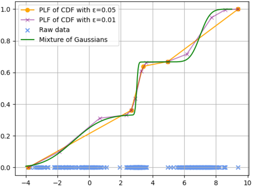
Figure 2: Samples (blue) drawn from a mixture of three Gaussian CDFs (green, log-likelihood of $-640.18$), the CDF approximated by a PLF with $\epsilon=0.05$ (orange, log-likelihood of $-685.91$) and the CDF approximated by a PLF with $\epsilon=0.01$. (purple, log-likelihood of $-624.49$) The hinges of the PLF are marked by orange dots and purple crosses.

For several reasons the use of a PLF as a regressor of the CDF of a probability distribution is appealing. (1) the concatenation of linear functions is very general, so that a PLF is capable of approximating functions of arbitrary shape and precision, and thus the resulting CDF can be considered free of model assumptions. (2) computations, manipulations and interpretations are intuitive and simple, and (3), there are efficient algorithms to acquire PLFs, such as MARS (Friedman, 1991). And (4) individual pieces can be learnt independently on partitions of the data and composed afterwards to form the final distribution. Figure 2 shows an example of a mixture of three Gaussian distributions and the approximation of its CDF in the form of a PLF that has been acquired from samples drawn. The Figure shows that the PLF is not only similar to the CDF of the three Gaussian distributions, but also competitive in terms of the likelihood.

3.2 Efficient Learning of Cumulative Distributions

In this section, we introduce an efficient algorithm for fitting CDFs in the form of PLFs. It is based on recursive partitioning of the data set $\widetilde{\mathcal{D}}$ and inspired by regression tree learning (Breiman et al., 2017a). Starting with $\widetilde{\mathcal{D}}$, a point $\left<d_{i^{*}},\gamma_{i^{*}}\right>\in\widetilde{\mathcal{D}}$ is determined, which minimizes the mean squared error (MSE) of a PLF of the form

$$f(d)=\left\{\begin{array}[]{ll}f_{1}(d)&\text{ if }d_{1}\leq d\leq d_{i^{*}}\\ f_{2}(d)&\text{ if }d_{i^{*}}\leq d\leq d_{N}\end{array}\right.,$$ (23)

for all $d\in\widetilde{\mathcal{D}}$. This process is recursively repeated on the subsets $\widetilde{\mathcal{D}}_{1}=\left\{d_{1},\ldots,d_{i^{*}}\right\}$ and $\widetilde{\mathcal{D}}_{2}=\left\{d_{i^{*}},\ldots,d_{N}\right\}$ until an error bound $\varepsilon$ is being undercut. Note that, if $\varepsilon=0$, the process will terminate when all points in $\widetilde{\mathcal{D}}$ have been selected as an optimal split point once. In this case, the learnt PLF reaches the highest possible likelihood, where every point is perfectly matched. The set of all points represents the interval boundaries of the PLF. The CDF-Learn algorithm is listed in Algorithm 1. MSE$(\mathcal{D})$ determines a function that returns the MSE of all points in $\mathcal{D}$ applied to a linear function through the minimal and maximal points in $\mathcal{D}$. The CDF-Learn pass yields the hinge points in $\widetilde{\mathcal{D}}$ that can be connected to form a linear spline of the CDF. The CDF is constantly 0 for all $d<\min\mathcal{D}$ and constantly 1 for all $d\geq\max\mathcal{D}$.

Algorithm 1 CDF-Learn

$\widetilde{\mathcal{D}}=\left\{\langle d_{i},\gamma_{i}\rangle\right\}$, a sorted set of $\gamma_{i}$-quantiles a set of hinge points of a PLF MSE$(\widetilde{\mathcal{D}})<\varepsilon$$\emptyset$Determine $\widetilde{\mathcal{D}}^{i^{*}}=\left\langle\widetilde{\mathcal{D}}_{1}^{i^{*}},\widetilde{\mathcal{D}}_{2}^{i^{*}}\right\rangle$, with

$$\widetilde{\mathcal{D}}_{1}^{i^{*}}=\left\{d_{1},\ldots,d_{i^{*}}\right\},\widetilde{\mathcal{D}}_{2}^{i^{*}}=\left\{d_{i^{*}},\ldots,d_{N}\right\},$$

such that ${i^{*}}=\operatorname*{\text{arg}\,\text{min}}_{i}{\mathds{E}\left(\text{MSE}\left(\widetilde{\mathcal{D}}^{i^{*}}\right)\right)}$$\{i^{*}\}\cup\textsc{CDF-Learn}(\widetilde{\mathcal{D}}_{1}^{i^{*}})\cup\textsc{CDF-Learn}(\widetilde{\mathcal{D}}_{2}^{i^{*}})$

3.3 Reasoning about Cumulative Distributions

A-priori reasoning In the previous section we introduced QPDs as a model-free representation of probability distributions and outlined the advantages of learning the respective CDF. Representing the CDF $F$ directly is advantageous over using the PDF, as marginal probabilities $P\!\left(X\leq x_{0}\right)$ and $P\!\left(X>x_{0}\right)$ can be obtained directly by evaluating $F$ without the computationally expensive step of integrating the PDF. Prior probabilities over intervals $[x_{l},x_{u}]$ can be computed by $P\!\left(x_{l}\leq X\leq x_{u}\right)=F(x_{u})-F(x_{l})$.

A-posteriori reasoning The calculation of a posterior $P\!\left(\!\begin{array}[]{c|c}\begin{array}[]{c}X\end{array}&\begin{array}[]{c}x_{l}\leq X\leq x_{u}\end{array}\end{array}\!\right)$ can be implemented in a similarly straightforward fashion. By decomposing the piecewise linear CDFs according to the posteriors’ condition, the distribution now represents only the required interval $[x_{l},x_{u}]$. Simply cropping and extracting a part of the function at the interval boundaries would leave us with an invalid QPD, since in most cases it will not represent probabilities ranging from $0.0$ to $1.0$. To normalize the distribution, the cropped part of the function is shifted to the base axis and stretched such that the properties of a valid distribution function are restored, i.e. $F(x_{l})$ and $F(x_{u})$ will evaluate to $0.0$ and $1.0$, respectively.

Confidence-rated output In many practical applications, obtaining a mere predictive value of a target variable is insufficient. Especially in safety-critical applications, it is crucial that predictions can have a confidence value attached expressing their dependability. For example, it is useful to report a confidence interval that encompasses the expectation of a variable $X$, $\mathds{E}(X)$, with a certain probability – the confidence level. In order to compute such a confidence interval $[x_{l},x_{u}]$ given a confidence level $\vartheta$, the inverse of the CDF, also called percent point function (PPF) can be used,

$$F^{-1}\left(F\left(\mathds{E}(X)\right)-\frac{\vartheta}{2}\right)\leq\mathds{E}(X)\leq F^{-1}\left(F\left(\mathds{E}(X)\right)+\frac{\vartheta}{2}\right).$$ (24)

In the case of PLFs, inverting the CDF is cheap and involves only the inversion of every linear component of the CDF. In the Experiments section, we present an example of confidence-rated outputs in JPTs.

3.4 Learning and Reasoning in Symbolic Domains

Probability distributions over symbolic variables are represented by histograms over the domains of the respective variables. If a path from the root of the tree to a leaf node contains a decision node constraining a symbolic variable, it is superfluous to store prior distributions over the respective variables in the leaves of the respective subtree, the impurity (entropy) of the variable is minimal already. In order to compute the leaf-conditionals $P\!\left(\!\begin{array}[]{c|c}\begin{array}[]{c}q_{i}\end{array}&\begin{array}[]{c}\lambda,e_{i}\end{array}\end{array}\!\right)$ in Eq. 18 for all symbolic variables $X_{i}$, it is sufficient to eliminate the inadmissible values of $X_{i}$ from the respective domain and re-normalize the histogram distribution.

4 Experiments

Figure 3: Expectations $\mathds{E}(X_{1}),\ldots,\mathds{E}(X_{64})$ over the probability distributions in the 14 leaf nodes of a learnt JPT (minimum 100 samples in each leaf). The clusters represented by the images in the leaf nodes reasonably match the associated class labels, which are displayed above the upper row and below the bottom row.

In recent years, various approaches for representing and learning probability distributions have been proposed, each of which is based on a specific set of constraints and assumptions (cf. Section Related Work). It is therefore difficult if not impossible to provide reasonable and robust evaluation criteria for comparing the predictive performance of a joint distribution learnt with different models.

Likelihood, on the one hand, is a well-known measure for a model’s ability to fit a data set. However, computing the exact likelihood in most previous works strongly depends on the model assumptions made and the preprocessing of the data sets. As – to the best of our knowledge – JPTs are the first approach that allows for hybrid symbolic/continuous model-free, joint probability distributions without prior assumptions, a direct comparison with previous works (Gens & Pedro, 2013; Dang et al., 2020; Vergari et al., 2021) is difficult if not impossible.

We additionally evaluate JPTs by comparing their predictive performance with respect to each variable in an experiment to a discriminative approach that has been trained on the respective variable exclusively with the same representational complexity (e.g. the number of samples in a leaf node). This is a relatively hard setup, because the single JPT model is to compete with specialized discriminative models, which are allowed to tailor their representational resources to one particular variable.

MNIST Data Set

Another popular dataset for ML model evaluation is known as MNIST (LeCun & Cortes, 2010). This dataset contains images of the digits 0 to 9, as written by various people. The images’ dimensions are 8$\times$8 and have grayscale values in the range 0-255. Traditionally, the task in this dataset is to correctly assign one of the labels 0-9 to every image in the collection, which is a discriminative problem statement. In this experiment, we demonstrate that JPTs can perform both discriminative classification tasks and generative sample generation. The learnt JPT comprises 14 leaves, whose expectation over the 65 variables are shown in Figure 3. It can be seen that the expected value over the pixel values reasonably matches the expectation over the class labels. A visualization of the tree structure itself can be found in the appendix.

Regression

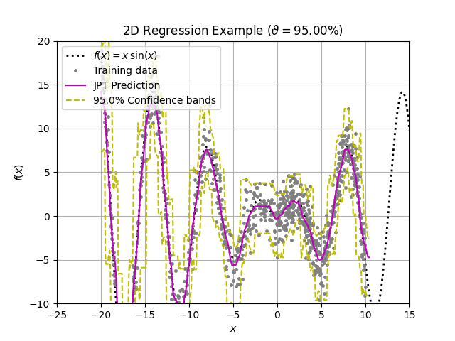
Figure 4: Regression fitting the function $f(x)=x\sin x$: The ground truth function $f(x)$ is shown in dotted gray, the training samples with Gaussian noise as gray dots, the prediction $\mathds{E}(y\!\mid\!x,\vartheta\!=\!.95)$ given by the learnt JPT in purple, and the yellow dashed lines represent the upper and lower percentiles of the prediction.

In this experiment, we demonstrate that JPTs can be used to accurately perform non-linear regression analyses, for which traditionally popular methods like ordinary least squares (OLS), regression trees (RT), or neural network models are chosen. We chose as ground truth regressor function $f(x)=x\sin x$, from which we sampled 1000 data points uniformly distributed with additive Gaussian noise. Regression analysis with joint distributions in JPTs can be achieved by evaluating the expected value of $y$ given the value of $x$, $\mathds{E}(y\!\mid\!x,\vartheta)$, as an estimate of $f(x)$, where $\vartheta$ is a confidence level that is used to calculate the confidence bounds of the answer as described in Section 3.3. Figure 4 shows the ground thruth, the sampled training data, the JPT prediciton as well as its upper and lower confidence bands. A quantitative comparison to CART is shown in Table 1.

# samples.	JPT	CART
20.0%	3.0041032	4.821578
10.0%	2.1888970	4.0494846
5.00%	1.6213786	2.3802814
2.00%	1.2783260	1.3080680
1.00%	0.7854674	0.9564107

Table 1: MAE (lower is better) for predictions in the regression experiment using JPT and CART with different learning parameters. ‘# samples’ denotes the fraction of available data samples that need to be covered by every leaf node.

Airline Departure Delay

JPTs can efficiently be learnt even with very large datasets. As an example, we are using the publicly available Airlines Departure Delay Prediction dataset provided by OpenML (Vanschoren et al., 2013). This dataset is particularly of interest, as it comprises 10 million instances each of which consists of 7 mixed-type feature values (3 nominal, 4 numeric). There are no missing values in that dataset. The results in Table 2 show that even though the JPT model represents all variables as opposed to the specialized CART models each of which only represents one variable, the JPT performs comparably well on all of the 7 variables and even outperforms the CART models in three of them. This is remarkable, because it shows, that JPTs can compete with specialized discriminative models.

Num. Variable	JPT	(+/-)	CART	(+/-)
DayOfWeek	1.89726	0.0118047	1.70767	0.00376937
CRSDepTime	144.518	0.615262	163.463	0.550986
Distance	293.35	2.82525	397.128	2.83425
CRSArrTime	139.678	0.825618	172.927	0.6609

Sym. Variable	JPT	(+/-)	CART	(+/-)
UniqueCarrier	0.178936	0.000313542	0.200474	0.000179531
Origin	0.0639007	3.28761e-05	0.0967244	1.47472e-05
Dest	0.0629808	1.9464e-05	0.0966721	1.41371e-05

Table 2: Experimental results on the Airline dataset: MAE (lower is better) and deviations of the numeric variables of JPT and CART (top) and F-score (higher is better) and deviation of the symbolic variables (bottom).

Empirical Evaluation

We conducted an extensive evaluation of JPTs on eight popular datasets from the UCI machine learning repository (Dua & Graff, 2017), in which we learnt JPTs with different hyperparameters and determined the size of the resulting models as well as the likelihoods they achieve. As a hyperparameter for learning, we varied the minimum number of samples in each leaf node to different portions of the available training data to induce different levels of model complexity. The evaluation has been conducted on test sets created by randomly sampling 10% of the data. Our experiments show that, with increasing complexity (i.e. decreasing minimum number of samples per leaf), the achieved likelihood of the learnt models reliably increases significantly both in the training set and in the test set. The detailed experimental results are listed in Table 3 in the appendix. The rightmost column contains the number of test samples with 0 likelihood. This typically happens in model-free distributions where test samples may lie outside the convex hull of the training data and the CDF-Learn algorithm assigns 0 probability mass to these regions.

5 Discussion

Joint probability distributions have great potential to serve as powerful problem-solving tools for machine learning applications. As opposed to most methods in the field of ML, joint distributions do not rely on dedicated input and output variables but can be queried for any aspect contained in the model given any evidence. Most existing methods, however, require strong assumptions that all variables are either symbolic or numeric or that their distributions have the same functional form. This makes the accompanying methods tailored to the specific densities. However, in many real-world problems, the semantics of variables calls for support of heterogeneous modalities of both numeric and categorical variables in a single model. JPTs meet this requirement of hybrid symbolic and subsymbolic reasoning, which has also been identified as one of the key demands of future AI applications (Marcus & Davis, 2019). A further significant advantage of JPTs over state-of-the-art PGMs is that JPTs do not rely on assumptions about dependencies or families of distributions at all. The variable dependencies are represented by the model structure that is generated as a byproduct of the learning procedure and the use of piecewise linear functions to approximate the CDFs of numeric variables allows highest flexibility with minimal model assumptions. The tree structure itself consists of conjunctions of variable constraints, each of which describes a specific subregion in the problem space. This makes the model structure interpretable and understandable for humans, and, as a consequence, its allows transparent reasoning and more robust, more traceable, and more explainable decision making (Goebel et al., 2018). The practical applicability of classic PGM is impeded by their representational and computational complexity that the models typically imply. The inferential complexity is $\#P$-complete in the general case (Koller & Friedman, 2009) and learning is intractable since it involves inference. To circumvent these computational challenges, strong assumptions about variable independence and approximate inference mechanisms have to be adduced. In JPTs, inference is exact and can be performed in linear time with respect to the model size, i.e. the number of leaves in the tree. In addition, it is easy to limit the complexity of the model by, for instance, the computational resources that are available. This makes JPTs extremely flexible, scalable and parallelizable. To the best of our knowledge, JPTs are the only shallow deterministic probablistic circuit, such that the circuit remains tractable for MPE inference.

In summary, we argue that JPTs address a selection of properties of machine learning methods that have been identified as pivotal challenges of AI and ML in the literature of recent years. In this section, we reviewed a selection thereof and discussed in a qualitative manner, in which way JPTs are capable of addressing these desiderata. For a more detailed discussion of activities and methods in a typical lifecycle of ML models we refer to the survey by (Ashmore et al., 2021).

6 Related Work

The field of probabilistic learning and reasoning is an important and actively investigated field of AI, and many works have been presented in the past years, which aim at making probabilistic models more tractable. (Poon & Domingos, 2011) represent the partition function of PGMs by introducing multiple layers of hidden variables by a deep architecture called sum-product networks (SPN). SPNs are rooted directed acyclic graphs, whose root values represent an unnormalized probability distribution and can be learnt recursively by either splitting it into a product of SPNs over independent sets of variables or into a sum of SPNs learned from subsets of the instance, if they cannot be found. SPNs perform approximate inference in the case of cyclic dependencies. Otherwise cycles have to be replaced by multivariate distributions whose representation is generally untractable (Gens & Pedro, 2013). As opposed to SPNs, JPTs do not rely on a dependency model prior to learning and support explainable reasoning in both symbolic and continuous variable domains. Contrasted with probabilistic circuits (PC), JPTs’ dependency model is learnt automatically from data and can express distributions without any model assumptions (Shah et al., 2021). In general, all PGMs postulate a rigid dependecy model that must be known before learning the model parameters and learning the structure of such a model imposes an additional NP-hard problem. In JPTs, the dependency model is automatically learned from the data while no model needs to be specified in advance. Like JPTs, cutset networks (Rahman et al., 2014) do recursive partitioning, but fit arbitrary Bayesian networks in the partitions. Cutset networks, however, are bound by the complexity of the Bayesian networks in the leaves and lack the ability to generally represent continuous variables. JPTs thus can be considered generalizations of both SPNs, PCs and CNs without the necessity to pre-define the model structure. (Bishop, 1994) introduces Mixture Density Networks (MDNs), which combine conventional neural networks with mixture density models. MDNs provide a general framework modeling conditional probability densities of the output variables, thus enabling a multi-valued mapping. Similarly to JPTs, MDNs are mixture models representing distributions over symbolic and subsymbolic variables. However, in contrast to MDNs, JPTs are generative models representing joint distributions over all variables instead of conditional probability densities of the output variables, which limits MDNs to be discriminative. Additionally, JPTs profit from the benefits of white-box tree structures that are intuitively interpretable, offer explainable decisions and allow efficient learning and reasoning. (Bishop & Svensén, 2012) use variational inference on Hierarchical Mixture of Experts (HME) to provide a Bayesian treatment of the model. It can be used to solve multi-dimensional regression problems and is expected to also work on binary classification problems. The HMEs often find local maxima which are not necessarily good solutions which the authors try to overcome by using multiple runs to select the best optima. However, this may be infeasible for large datasets. For a more detailed review of mixture-of-expert models we refer to in Yuksel et al. (2012).

7 Conclusions

We introduced Joint Probability Trees (JPT), which are tree-based representations that allow the compact representation and efficient learning of and reasoning about joint probability distributions. As opposed to PGMs, JPTs support learning and reasoning in hybrid domains, i.e. they allow to coalesce numeric and symbolic variables in one single model in a sound and consistent way. A key feature of JPTs is that the dependencies among variables are represented in a tree structure, whose leaves maintain univariate prior distributions over all variables. For numeric variables, we propose quantile-parameterized distributions, which can be regarded as model-free representations of arbitrary numeric distributions. Our experiments show that JPTs are able to accurately learn and represent complex interactions between many variables, while keeping interpretability and scalability. We argue that the challenges that we address with JPTs will be key in making the transition from narrow, specialized expert systems to hybrid, high performance AI systems and in pushing todays computer systems towards more generally intelligent and more robust and reliable decision making.

8 Appendix

8.1 Empirical Evaluation

Dataset	Min samples per leaf	Model Size	Average Train Log-Likelihood	Average Test Log-Likelihood	0-likelihood Test Samples
IRIS Dataset Examples: 150 Variables: 5	90%	23	-5.45	-5.63	-
	40%	46	-3.54	-3.33	-
	20%	94	-2.16	-2.66	20%
	10%	184	-1.37	-1.91	27%
	5%	353	-0.18	-1.2	67%
	1%	679	6.11	-	100%
Adult Dataset Examples: 32561 Variables: 15	90%	1472557	-55.46	-54.98	49%
	40%	2945118	-53.79	-53.07	58%
	20%	5890233	-52.96	-52.45	64%
	10%	11780477	-51.17	-50.18	70%
	5%	22088384	-50.13	-50.25	81%
	1%	94243769	-41.57	-42.96	93%
Dry Bean Dataset Examples: 13611 Variables: 17	90%	476858	-17.49	-16.98	95%
	40%	953709	-12.13	-13.23	95%
	20%	1430565	-9.80	-10.68	95%
	10%	3814841	-4.91	-6.75	95%
	5%	7629662	-2.31	-4.11	95%
	1%	36717612	2.41	0.85	96%
Wine Dataset Examples: 178 Variables: 13	90%	1550	-18.97	-19.83	56%
	40%	3101	-17.06	-18.69	83%
	20%	6197	-13.42	-14.9	94%
	10%	12417	-10.98	-12.46	94%
	5%	24824	-6.74	-	100%
	1%	207028	41.22	-	100%
Wine Quality Dataset Examples: 6497 Variables: 13	90%	67	-9.50	-9.8	-
	40%	138	-8.10	-8.34	1%
	20%	204	-7.60	-7.68	1%
	10%	479	-6.48	-6.57	2%
	5%	1072	-5.67	-5.85	4%
	1%	5307	-3.08	-3.82	12%
Bank and Marketing Dataset Examples: 45211 Variables: 17	90%	116433	-34.60	-34.64	07%
	40%	232866	-34.50	-34.54	8%
	20%	465732	-34.31	-34.32	12%
	10%	815031	-33.00	-32.77	20%
	5%	1630062	-32.43	-32.08	32%
	1%	7335279	-30.46	-29.45	73%
Car evaluation Dataset Examples: 1728 Variables: 6	90%	21	-6.89	-7.03	-
	40%	21	-6.89	-7.03	-
	20%	63	-6.52	-6.62	-
	10%	147	-6.48	-6.61	-
	5%	231	-6.45	-6.59	-
	1%	1249	-6.38	-6.66	-
Abalone Dataset Examples: 4177 Variables: 9	90%	64	0.09	-0.04	-
	40%	134	3.65	3.66	-
	20%	208	5.34	5.11	-
	10%	482	8.14	8.05	2%
	5%	1034	9.32	9.28	3%
	1%	5502	11.34	10.74	18%

Table 3: Results of the evaluation of JPTs on eight benchmark data sets of the UCI machine learning repository (Dua & Graff, 2017) for different hyperparameters. “Min samples per leaf” means that at least the respective percentage of data points available for training must be represented by any leaf of the tree. “Min samples per leaf”=90% thus results in a JPT with only one leaf, i.e. a set of independent prior distributions over all variables considered. “0-likelihood test samples” determines the percentage of test samples with 0 likelihood. This may happen to samples lying outside the convex hull of the training data, where 0 probability mass is assigned by the CDF-Learn algorithm.

8.2 JPT Example - Tree

Figure 5: The ground truth distribution of the toy data set in Section 2.3.

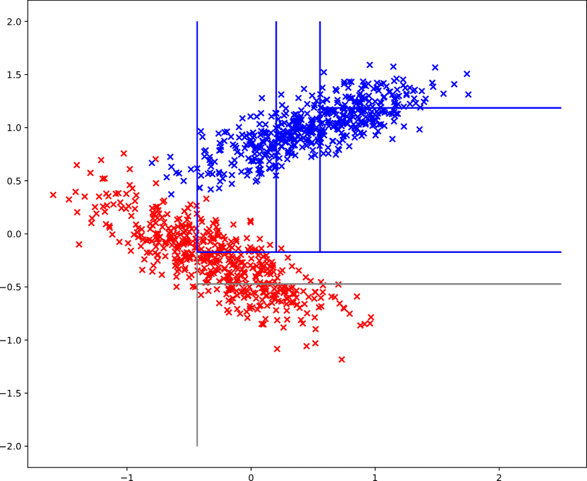
Figure 6: The scatterplot of the underlying toy data set in Section 2.3.

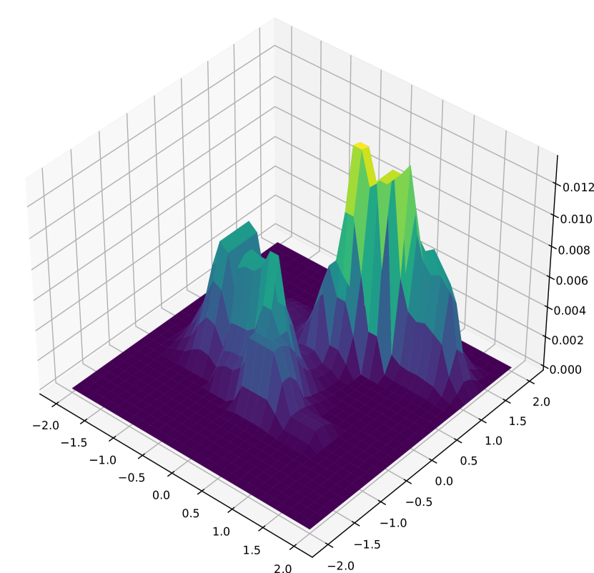
Figure 7: The plot of the marginal joint distribution $P(X,Y)$ of the toy data set in Section 2.3.

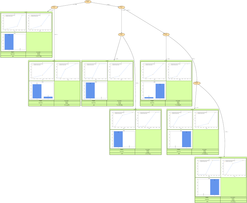
Figure 8: The JPT structure learnt using the toy data set in Section 2.3.

8.3 MNIST - Tree

Figure 9: The JPT structure learnt using the MNIST data set.

References

- Ashmore et al. (2021) Ashmore, R., Calinescu, R., and Paterson, C. Assuring the machine learning lifecycle: Desiderata, methods, and challenges. ACM Computing Surveys (CSUR), 54(5):1–39, 2021.
- Besag (1975) Besag, J. Statistical analysis of non-lattice data. Journal of the Royal Statistical Society: Series D (The Statistician), 24(3):179–195, 1975.
- Bishop (1994) Bishop, C. M. Mixture density networks. 1994.
- Bishop & Svensén (2012) Bishop, C. M. and Svensén, M. Bayesian hierarchical mixtures of experts. arXiv preprint arXiv:1212.2447, 2012.
- Breiman et al. (1984) Breiman, L., Friedman, J., Olshen, R., and Stone, C. Cart. Classification and Regression Trees; Wadsworth and Brooks/Cole: Monterey, CA, USA, 1984.
- Breiman et al. (2017a) Breiman, L., Friedman, J. H., Olshen, R. A., and Stone, C. J. Classification and regression trees. Routledge, 2017a.
- Breiman et al. (2017b) Breiman, L., Friedman, J. H., Olshen, R. A., and Stone, C. J. Classification and regression trees. Routledge, 2017b.
- Chater et al. (2006) Chater, N., Tenenbaum, J. B., and Yuille, A. Probabilistic Models of Cognition: Conceptual Foundations. Trends in Cognitive Sciences, Special Issue: Probabilistic Models of Cognition, 10(7), 2006.
- Dang et al. (2020) Dang, M., Vergari, A., and Broeck, G. Strudel: Learning structured-decomposable probabilistic circuits. In International Conference on Probabilistic Graphical Models, pp. 137–148. PMLR, 2020.
- Dua & Graff (2017) Dua, D. and Graff, C. UCI machine learning repository, 2017. URL http://archive.ics.uci.edu/ml.
- Friedman (1991) Friedman, J. H. Multivariate adaptive regression splines. Ann. Statist, 1991.
- Gens & Pedro (2013) Gens, R. and Pedro, D. Learning the structure of sum-product networks. In International conference on machine learning, pp. 873–880. PMLR, 2013.
- Goebel et al. (2018) Goebel, R., Chander, A., Holzinger, K., Lecue, F., Akata, Z., Stumpf, S., Kieseberg, P., and Holzinger, A. Explainable ai: The new 42? In Holzinger, A., Kieseberg, P., Tjoa, A. M., and Weippl, E. (eds.), Machine Learning and Knowledge Extraction, pp. 295–303, Cham, 2018. Springer International Publishing. ISBN 978-3-319-99740-7.
- Griffiths et al. (2008) Griffiths, T. L., Kemp, C., and Tenenbaum, J. B. The Cambridge Handbook of Computational Cognitive Modeling, chapter Bayesian Models of Cognition. Cambridge University Press, 2008.
- Jain (2012) Jain, D. Probabilistic Cognition for Technical Systems: Statistical Relational Models for High-Level Knowledge Representation, Learning and Reasoning. PhD thesis, Technische Universität München, 2012. URL http://mediatum.ub.tum.de/node?id=1096684&change_language=en.
- Keelin & Powley (2011) Keelin, T. W. and Powley, B. W. Quantile-parameterized distributions. Decision Analysis, 8(3):206–219, September 2011. ISSN 1545-8490. doi: 10.1287/deca.1110.0213. URL https://doi.org/10.1287/deca.1110.0213.
- Knill & Pouget (2004) Knill, D. C. and Pouget, A. The Bayesian Brain: The Role of Uncertainty in Neural Coding and Computation. Trends in Neurosciences, 27(12), 2004.
- Koller & Friedman (2009) Koller, D. and Friedman, N. Probabilistic Graphical Models: Principles and Techniques. Adaptive computation and machine learning. MIT Press, 2009. ISBN 9780262013192. URL https://books.google.de/books?id=7dzpHCHzNQ4C.
- LeCun & Cortes (2010) LeCun, Y. and Cortes, C. MNIST handwritten digit database. 2010. URL http://yann.lecun.com/exdb/mnist/.
- Loh (2014) Loh, W.-Y. Fifty years of classification and regression trees. International Statistical Review, 82(3):329–348, 2014.
- Marcus & Davis (2019) Marcus, G. and Davis, E. Rebooting AI – Building Artificial Intelligence we can trust. Pantheon, 2019.
- Murphy (2022) Murphy, K. P. Probabilistic Machine Learning: An introduction. MIT Press, 2022. URL probml.ai.
- Poon & Domingos (2011) Poon, H. and Domingos, P. Sum-product networks: A new deep architecture. In 2011 IEEE International Conference on Computer Vision Workshops (ICCV Workshops), pp. 689–690. IEEE, 2011.
- Quinlan (1993) Quinlan, R. C4. 5. Programs for machine learning, 1993.
- Rahman et al. (2014) Rahman, T., Kothalkar, P., and Gogate, V. Cutset networks: A simple, tractable, and scalable approach for improving the accuracy of chow-liu trees. In Joint European conference on machine learning and knowledge discovery in databases, pp. 630–645. Springer, 2014.
- Shah et al. (2021) Shah, N., Olascoaga, L. I. G., Zhao, S., Meert, W., and Verhelst, M. Piu: A 248gops/w stream-based processor for irregular probabilistic inference networks using precision-scalable posit arithmetic in 28nm. In 2021 IEEE International Solid- State Circuits Conference (ISSCC), volume 64, pp. 150–152, 2021. doi: 10.1109/ISSCC42613.2021.9366061.
- Vanschoren et al. (2013) Vanschoren, J., van Rijn, J. N., Bischl, B., and Torgo, L. Openml: Networked science in machine learning. SIGKDD Explorations, 15(2):49–60, 2013. doi: 10.1145/2641190.2641198. URL http://doi.acm.org/10.1145/2641190.2641198.
- Vergari et al. (2021) Vergari, A., Choi, Y., Liu, A., Teso, S., and Van den Broeck, G. A compositional atlas of tractable circuit operations for probabilistic inference. Advances in Neural Information Processing Systems, 34:13189–13201, 2021.
- Yuksel et al. (2012) Yuksel, S. E., Wilson, J. N., and Gader, P. D. Twenty years of mixture of experts. IEEE transactions on neural networks and learning systems, 23(8):1177–1193, 2012.