Abstract

The CDF collaboration has released a new measurement of the $W$ boson mass using their complete data set with 8.8 fb^-1 in $p\bar{p}$ collisions. This result deviates from the Standard Model prediction by around 7$\sigma$. We explain how the two Higgs doublet model (2HDM) with vector-like quarks is affected by the recently discovered W boson mass. In our study, we include both theoretical constraints such as perturbative unitarity and vacuum stability as well as a number of experimental constraints. We also look into how the effective mixing angle, measured by the SLD collaboration in addition to the CDF W-boson mass, is used to determine the $S$ and $T$ parameters. In the alignment limit, we investigate the case where the lighter CP-even neutral Higgs boson of the 2HDM is the one found at the LHC and demonstrate how the parameter space of the 2HDM type II in the presence of vector-like quarks is constrained. It is found that in most cases, there is a cancellation between the 2HDM and vector-like quarks contributions, which enlarges the parameter space of both models.

1 Introduction

Since the advent of the precise measurement programs at SLD, LEP, and Tevatron, ElectroWeak Precision Observables (EWPOs), such as the W boson mass, the effective mixing angle $\sin^{2}\theta_{eff}$, and the Z boson width, among others, have been used to precisely assess the viability of the Standard Model (SM) of particle physics. It turns out that some Beyond SM (BSM) extensions can be severely constrained by these EWPOs. Using their whole data set of 8.8 fb^-1 in $p\bar{p}$ collisions at CDF detector, the CDF collaboration recently released a new measurement of the $W$ boson mass (Fermilab Tevatron) [1]:

$$M^{\mathrm{CDF}}_{W}=80.4335\pm 0.0094~{}\mathrm{GeV}$$ (1)

This measurement is more precise than all prior measures put together, and it is highly accurate. In addition, the new CDF value agrees with some previous W mass measurements, but there are also some discrepancies [2]. Based on complex SM radiative correction calculations that relate the W mass to other SM particles such as the Higgs boson and the top masses, the SM prediction for the W mass at the per mille level is given by [2]:

$$M_{W}^{\mathrm{SM}}=80.357\pm 0.006\mathrm{GeV}$$ (2)

It is clear that the above CDF measurement depicts a remarkable 7$\sigma$ disagreement with the SM prediction. Several analyses have been presented in this direction, including those involving the 2HDM [3], the triplet Higgs model [4] and other SM extensions [5].

In the past, during the LEP era, it was well known that the global fit of SM predictions to LEP data was used to predict the existence of a heavy top quark and a relatively light Higgs boson well before their discovery at the Tevatron and LHC, respectively. Although the CDF measurement needs to be confirmed, it is quite likely that the difference between the experimental value and the expected SM value is due to a non-decoupled new interactions or new particles. If this is the case and if the scale of the new interaction is not too high, there is a chance that these new particles will show up in future experiments.

The SM of particle physics has been highly successful in explaining all observed phenomena at LEP and the LHC. However, there are several indications that the SM is only an effective theory of a more fundamental and complete theory that addresses its weaknesses, such as the dark matter puzzle, the need for additional sources of CP violation to explain the baryon asymmetry in the universe, and the issues with neutrino mass and mixing. Most BSM models predict additional vector-like fermions (quarks and leptons) and/or additional Higgs bosons in their spectrum [6, 7]. It is now well established that SM-like chiral fermions(a fourth generation of quarks) have been excluded by high precision measurements of Higgs production rates at the LHC [10, 9]. In the present study, we focus on new states of matter that are spin 1/2 particles and transform as triplets under color. However, unlike SM quarks, their left- and right-handed couplings have the same Electro-Weak (EW) quantum numbers, called Vector-Like Quarks (VLQs) [11, 7, 6, 12, 13, 14, 15, 16, 17, 18, 19, 20, 21, 22, 23, 24, 25, 26]. This class of models is well motivated since they show up in many composite Higgs models [27, 28, 30, 29, 31, 32] as well as in various little Higgs models [33, 34, 35]. We will also consider an extension of the SM that includes both VLQs and an additional Higgs doublet (as stated in reference [7]).
Several searches for VLQs have been carried out by the ATLAS and CMS collaborations, both from single production via an electroweak interaction and from pair production through the strong interaction. No significant deviation from the expected background of the SM has been observed, and exclusion limits have been set on the masses of the VLQs. Both the ATLAS and CMS experiments have searched $T$ and $B$ production at $\sqrt{s}=8$ TeV and $\sqrt{13}$ TeV, spanning practically all production and decay channels. With an integrated luminosity of 138 $fb^{-1}$, CMS presented a search [36] for $T\bar{T}$ and $B\bar{B}$ pair production of VLQs, excluding masses up to 1.54 TeV (1.56 TeV) for vector-like T and B quarks, respectively, at a 95% confidence level, depending on their branching ratio scenarios. For vector-like T quarks, masses below 1.48 TeV are excluded in any branching fraction scenario, i.e. decay to the final states tZ, bW, and th, where h is the SM Higgs boson. Analogous exclusion limits by ATLAS [37] at $95\%$ confidence level have been set on the VLQs masses up to 1030 (1210) GeV for singlet (doublet) vector-like T quark and 1010 (1140) GeV for singlet (doublet) vector-like B quark. It is important to note that all these search limits are given with the assumption that VLQs decay only to third generation SM particles, and they can be lowered if the VLQs have a non-negligible coupling with the first and second generation SM quarks. Besides, if we consider 2HDM+VLQs, in this case, we will have the possibility for other new decay modes of VLQs to BSM Higgs bosons, such as the decay of vector-like T quark to $tH,tA$, and $bH^{\pm}$, and hence the previous exclusion limits can be further weakened down [7] where $A$, $H$ and $H^{\pm}$ are extra Higgs bosons predicted by the 2HDM.

The oblique parameters $S$, $T$ and $U$ represent important tools at the TeV scale that indicate the level of violation of the custodial isospin symmetry. They contribute significantly to electroweak radiative corrections. It is very well known that in the SM, $S=T=U=0$ at a reference point where the top quark and Higgs boson masses are fixed. Beyond the SM, these parameters are sensitive to new physics and hence measure their effects. The exact calculations of S, T and U oblique parameters are tedious and prone to error, with the help of public codes such as FeynArts, FormCalc, and LoopTools, an automated code has been introduced to improve the reliability of the calculations. In the current work, we present to the best of our knowledge, the first exact calculations of electroweak oblique parameters $S$ and $T$ in the 2HDM type II in the presence of singlets, doublets, and triplets vector-like quarks scenarios in the context of CP conserving case. Our results are given using the well-known scalar Passarino-Veltman functions [8]. We examine in detail the conditions that may affect the oblique parameters in our model, then study the impact of the new CDF result on the extra new quarks. The 2HDM+VLQs is a good candidate for analyzing the oblique parameters formalism because the model has new quarks and their couplings to gauge bosons are model-dependent.
This paper is organized as follows: In Section 2, we give a brief review of VLQs and 2HDM in terms of particle content and their mass. We also present how the W boson mass can be parameterized in terms of the oblique parameters $S$, $T$ and $U$. In Section 3, we show our numerical analysis within the 2HDM type II augmented by VLQs. We conclude in Section 4. Finally, in the appendix we present the contributions of the vector-like quarks to $S$, $T$ and $U$ parameters and we give the relevant couplings to our study and explain the CDF-II W-boson mass anomaly within the SM extended with VLQs.

2 Models description

2.1 VLQs

In this section, we introduce our parametrization and notation for VLQs . As low energy physics measurements severely limit the mixing of VLQs with the first and second generations, we only consider the scenario where the VLQs couple to the third-generation SM quarks. There are seven distinct possibilities of Vector-like $SU(2)_{L}$ multiplets with renormalizable couplings that are allowed to mix through Yukawa couplings with the SM quarks, i.e we have two electroweak singlets, three electroweak doublets and two electroweak triplets as indicated below:

$$T_{L,R}^{0}\,,\quad B_{L,R}^{0} \text{(singlets)}\,,$$

$$(T^{0}\,B^{0})_{L,R}\,,\quad(X^{0}\,T^{0})_{L,R}\,,\quad(B^{0}\,Y^{0})_{L,R} \text{(doublets)}\,,$$

$$(X^{0}\,T^{0}\,B^{0})_{L,R}\,,\quad(T^{0}\,B^{0}\,Y^{0})_{L,R} \text{(triplets)}\,.$$ (3)

Where the heavy quarks have the following electric charges: $Q_{T}=\frac{2}{3},Q_{B}=-\frac{1}{3},Q_{X}=\frac{5}{3}$, and $Q_{Y}=-\frac{4}{3}$. In the Higgs basis, the Yukawa Lagrangian may be expressed as:

$$-\mathcal{L}\,\,\supset\,\,y^{u}\bar{Q}^{0}_{L}\tilde{H}_{2}U^{0}_{R}+y^{d}\bar{Q}^{0}_{L}H_{1}D^{0}_{R}+M^{0}_{u}\bar{U}^{0}_{L}U^{0}_{R}+M^{0}_{d}\bar{D}^{0}_{L}D^{0}_{R}+\rm{h.c}.$$ (4)

where, $U_{R}\equiv(u_{R},c_{R},t_{R},T_{R})$ and $D_{R}\equiv(d_{R},s_{R},b_{R},B_{R})$ while $y^{u,d}$ are 3$\times$4 Yukawa matrices. In the scenario where the new heavy quarks couple to third generation, the physical mass eigenstates fields $(t,T)$ and $(b,B)$ can be obtained by rotating the gauge eigenstates through four unitary mixing matrices $U_{L,R}^{u}$ and $U_{L,R}^{d}$, which are parametrized as follows:

$$\left(\!\begin{array}[]{c}t_{L,R}\\ T_{L,R}\end{array}\!\right)=U_{L,R}^{u}\left(\!\begin{array}[]{c}t^{0}_{L,R}\\ T^{0}_{L,R}\end{array}\!\right)=\left(\!\begin{array}[]{cc}\cos\theta_{L,R}^{u}&-\sin\theta_{L,R}^{u}\\ \sin\theta_{L,R}^{u}e^{-i\phi_{u}}&\cos\theta_{L,R}^{u}\end{array}\!\right)\left(\!\begin{array}[]{c}t^{0}_{L,R}\\ T^{0}_{L,R}\end{array}\!\right)\,.$$ (5)

$$\left(\!\begin{array}[]{c}b_{L,R}\\ B_{L,R}\end{array}\!\right)=U_{L,R}^{d}\left(\!\begin{array}[]{c}b^{0}_{L,R}\\ B^{0}_{L,R}\end{array}\!\right)=\left(\!\begin{array}[]{cc}\cos\theta_{L,R}^{d}&-\sin\theta_{L,R}^{d}\\ \sin\theta_{L,R}^{d}e^{-i\phi_{d}}&\cos\theta_{L,R}^{d}\end{array}\!\right)\left(\!\begin{array}[]{c}b^{0}_{L,R}\\ B^{0}_{L,R}\end{array}\!\right)\,.$$ (6)

In the weak eigenstate basis, the mass terms for the top and bottom quarks and the VLQs can be extracted from

$$\mathcal{L}_{\text{mass}} = -\left(\!\begin{array}[]{cc}\bar{t}_{L}^{0}&\bar{T}_{L}^{0}\end{array}\!\right)\left(\!\begin{array}[]{cc}y_{33}^{u}\frac{v}{\sqrt{2}}&y_{34}^{u}\frac{v}{\sqrt{2}}\\ y_{43}^{u}\frac{v}{\sqrt{2}}&M^{0}\end{array}\!\right)\left(\!\begin{array}[]{c}t^{0}_{R}\\ T^{0}_{R}\end{array}\!\right)$$ (18)

$$-\left(\!\begin{array}[]{cc}\bar{b}_{L}^{0}&\bar{B}_{L}^{0}\end{array}\!\right)\left(\!\begin{array}[]{cc}y_{33}^{d}\frac{v}{\sqrt{2}}&y_{34}^{d}\frac{v}{\sqrt{2}}\\ y_{43}^{d}\frac{v}{\sqrt{2}}&M^{0}\end{array}\!\right)\left(\!\begin{array}[]{c}b^{0}_{R}\\ B^{0}_{R}\end{array}\!\right)+\text{h.c.},$$

Where $y_{ij}$ are the Yukawa couplings and $M^{0}$ is a bare mass term. For singlets and triplets, $y_{43}=0$, while for doublets, $y_{34}=0$. The unitary matrices will be specified in the case where the mass matrices are diagonal in the mass eigenstate basis.

$$U_{L}\,\mathcal{M}\,(U_{R})^{\dagger}=\mathcal{M}^{q}_{\text{diag}}\,,$$ (19)

with $\mathcal{M}$ are the mass matrices in Eq. (18) and $\mathcal{M}^{q}_{\text{diag}}$ are the diagonalized matrices given by.

$$\mathcal{M}^{t}_{\text{diag}}=\left(\!\begin{array}[]{cc}m_{t}&0\\ 0&m_{T}\end{array}\!\right)\quad\text{and}\quad\mathcal{M}^{b}_{\text{diag}}=\left(\!\begin{array}[]{cc}m_{b}&0\\ 0&m_{B}\end{array}\!\right)$$ (20)

Note that the two mixing angles $\theta_{L}$ and $\theta_{R}$ are not independent parameters. By using Eq. (19), and depending on the representation of the VLQs, one can find that:

$$\tan\theta_{R}^{q} = \frac{m_{q}}{m_{Q}}\tan\theta_{L}^{q}\quad\text{(singlets, triplets)}\,,$$

$$\tan\theta_{L}^{q} = \frac{m_{q}}{m_{Q}}\tan\theta_{R}^{q}\quad\text{(doublets)}\,,$$ (21)

with $(q,m_{q},m_{Q})=(u,m_{t},m_{T})$ and $(d,m_{b},m_{B})$.
Additionally, there are relationships between the mass eigenstates and angles that depend on the representation of the VLQs [6]

$${Doublets:} (T\,B): m_{T}^{2}(c_{R}^{u})^{2}+m_{t}^{2}(s_{R}^{u})^{2}=m_{B}^{2}(c_{R}^{d})^{2}+m_{b}^{2}(s_{R}^{d})^{2}$$ (22)

$$(X\,T): m_{X}^{2}=m_{T}^{2}(c_{R}^{u})^{2}+m_{t}^{2}(s_{R}^{u})^{2}$$

$$(B\,Y): m_{Y}^{2}=m_{B}^{2}(c_{R}^{d})^{2}+m_{b}^{2}(s_{R}^{d})^{2}$$

$${Triplets:} (X\,T\,B): m_{X}^{2}=m_{T}^{2}(c_{L}^{u})^{2}+m_{t}^{2}(s_{L}^{u})^{2}$$ (23)

$$\phantom{m_{X}^{2}}=m_{B}^{2}(c_{L}^{d})^{2}+m_{b}^{2}(s_{L}^{d})^{2}$$

From the above equations, it is easy to derive the following relationships:

$${m_{B}^{2}}=\frac{1}{2}\sin^{2}\left(2\theta^{u}_{L}\right)\frac{m_{T}^{2}-m_{t}^{2}}{m_{X}^{2}-m_{b}^{2}}+m_{X}^{2}$$

$$\sin(2\theta_{L}^{d})=\sqrt{2}\frac{m_{T}^{2}-m_{t}^{2}}{(m_{B}^{2}-m_{b}^{2})}\sin(2\theta_{L}^{u})$$ (24)

Similarly for the $(T\,B\,Y)$ triplet, we have:

$$m_{Y}^{2}=m_{B}^{2}(c_{L}^{d})^{2}+m_{b}^{2}(s_{L}^{d})^{2}$$

$$\phantom{m_{Y}^{2}}=m_{T}^{2}(c_{L}^{u})^{2}+m_{t}^{2}(s_{L}^{u})^{2}$$ (25)

We may therefore deduce the following relations:

$${m_{B}^{2}}=\frac{1}{8}\sin^{2}\left(2\theta^{u}_{L}\right)\frac{m_{T}^{2}-m_{t}^{2}}{m_{Y}^{2}-m_{b}^{2}}+m_{Y}^{2}$$

$$\sin(2\theta_{L}^{d})=\frac{m_{T}^{2}-m_{t}^{2}}{\sqrt{2}(m_{B}^{2}-m_{b}^{2})}\sin(2\theta_{L}^{u})$$ (26)

where the mixing between the top-quark and down-quark vector-like fermions is described by $c_{L,R}^{u,d}=\cos\,\theta_{L,R}^{u,d}$ and $s_{L,R}^{u,d}=\sin\,\theta_{L,R}^{u,d}$.
It can be easily inferred that all representations of the VLQs can be characterized by only two parameters, except for the $(T,B)$ top partner doublet model which requires three parameters. In our numerical analysis, the following input parameters will be used:

Representations Singlets Doublets Triplets $T$ $B$ $T\,B$ $X\,T$ $B\,Y$ $X\,T\,B$ $T\,B\,Y$ Parameters $m_{T},s_{L}^{u}$ $m_{B},s_{L}^{d}$ $m_{T},s_{R}^{u},s_{R}^{d}$ $m_{T},s_{R}^{u}$ $m_{B},s_{R}^{d}$ $m_{T},s_{L}^{u}$ $m_{T},s_{L}^{u}$

2.2 2HDM

One of the simplest extensions of the SM’s Higgs sector is the two Higgs doublet model (2HDM) which consist of adding a new Higgs doublet to the existing one in the SM. The most general scalar potential which is invariant under $SU_{L}(2)\times U_{Y}(1)$ and satisfy a discrete $Z_{2}$ symmetry $\phi_{1}\rightarrow+\phi_{1}$ and $\phi_{2}\rightarrow-\phi_{2}$, can be written as [38]

$$V(\phi_{1},\phi_{2}) = m_{11}^{2}(\phi_{1}^{\dagger}\phi_{1})+m_{22}^{2}(\phi_{2}^{\dagger}\phi_{2})-[m_{12}^{2}(\phi_{1}^{\dagger}\phi_{2})+\text{h.c.}]$$ (27)

$$+ \frac{1}{2}\lambda_{1}(\phi_{1}^{\dagger}\phi_{1})^{2}+\frac{1}{2}\lambda_{2}(\phi_{2}^{\dagger}\phi_{2})^{2}+\lambda_{3}(\phi_{1}^{\dagger}\phi_{1})(\phi_{2}^{\dagger}\phi_{2})~{}$$

$$+ \lambda_{4}(\phi_{1}^{\dagger}\phi_{2})(\phi_{2}^{\dagger}\phi_{1})+\frac{1}{2}\left[\lambda_{5}(\phi_{1}^{\dagger}\phi_{2})^{2}+\rm{h.c.}\right],$$

where $\lambda_{1,2,3,4,5}$ as well as $m_{11,22,12}^{2}$ are chosen to be real ensuring that the potential is CP conserving. If both Higgses $\phi_{1}$ and $\phi_{2}$ interact with all SM fermions, like in the SM, we end up with Flavour Changing Neutral Currents (FCNCs) at the tree-level in the Yukawa sector. For this purpose, a discrete $Z_{2}$ symmetry has been introduced to prevent the occurrence of large tree-level FCNCs [39, 38]. Moreover, based on the $Z_{2}$ symmetry assignment, there are four possible types of Yukawa sector. In this study, we concentrate on 2HDM Type II, where one doublet couples to down-type quarks and leptons, while the other couples to up-type quarks.

After EWSB takes place, we are left with five physical Higgs bosons: two CP-even $h$ and $H$ with $m_{h}<m_{H}$, one CP-odd $A$, and a pair of charged Higgs $H^{\pm}$. In our study, we assume that the light CP-even Higgs $h$ will be identified as the Higgs boson observed at the LHC, and we assume $m_{h}\approx 125$ GeV. The other parameters of the model are:

• $\tan\beta=v_{2}/v_{1}$ which is the ratio of the vevs.

• $\sin(\beta-\alpha)$ , where $\alpha$ is the mixing angle between the CP-even components of the Higgs fields

• $m_{12}^{2}$: $Z_{2}$ soft breaking term

• $m_{H,A,H^{\pm}}$: the physical masses of the extra Higgs bosons.

2.3 $W$ mass and ($S$, $T$, $U$) parameters

The $W$-boson mass $M_{W}$ is one of the significant EWPOs due to its precise experimental measurements. It can be calculated as a function of the oblique parameters $S$, $T$ and $U$ [41, 40]. The oblique parameters in 2HDM differ from those in the SM because of the additional contributions from the Higgs boson loops and the modified couplings of the SM-type Higgs bosons.

The W-boson mass can be calculated from the oblique parameters, which can be expressed as follows [42]:

$$\left.M_{W}^{2}=M_{W}^{2}\right\rvert^{SM}{}\left[1+\frac{\alpha(M_{Z})}{\left(c_{W}^{2}-s_{W}^{2}\right)}\left(-\frac{1}{2}S+c_{W}^{2}T+\frac{c_{W}^{2}-s_{W}^{2}}{4s_{W}^{2}}U\right)\right].$$ (28)

Where $c_{W}=\cos\theta_{W}$ and $s_{w}=\sin\theta_{W}$, $\theta_{W}$ is Weimberg angle. When compared to the contributions from $S$ and $T$, the contribution from the oblique parameter U is expected to be negligible in many new physics models. Hence, we present the results for $S$ and $T$ assuming $U=0$.
Additionally, it is possible to assess the impact of changes in the $W$-boson mass on the effective weak mixing angle $\sin^{2}\theta_{\mathrm{eff}}$, which is calculated as described in [43]:

$$\sin^{2}\theta_{eff}=\left.\sin^{2}\theta_{\mathrm{eff}}\right\rvert^{SM}{}-\alpha\frac{c_{W}^{2}s_{W}^{2}}{c_{W}^{2}-s_{W}^{2}}(T-\frac{s_{W}^{2}}{c_{W}^{2}}S+\frac{1}{2}U)$$ (29)

with the SM values $\left.M_{W}\right\rvert^{SM}{}=80.357$ GeV and $\left.\sin^{2}\theta_{\mathrm{eff}}\right\rvert^{SM}{}=0.231532$.
In the framework of 2HDM with VLQs, the oblique parameters $S$ and $T$ have two separate contributions: one from the VLQs and the other from the Higgs bosons in the 2HDM:

$$S_{SM+VLQs}=S_{SM}+S_{VLQs},\quad\ T_{SM+VLQs}=S_{SM}+S_{VLQs}$$

$$S_{2HDM+VLQs}=S_{2HDM}+S_{VLQs},\quad\ T_{2HDM+VLQs}=S_{2HDM}+S_{VLQs}$$ (30)

The detailed analytical formulations for $S_{2HDM,VLQs}$ and $T_{2HDM,VLQs}$ in terms of the Passarino-Veltman functions can be found in Appendix Acknowledgments. With the help of LoopTools [44, 45], the numerical evaluations of the scalar functions are carried out.

We compared our analytical expression for the contributions of 2HDM to $S$ and $T$ to those in [15] and [46] and found good agreement. In the case of singlet and doublet representations, the VLQs contributions can be computed with the use of Ref. [16]. This has been used for a number of VLQ models, as mentioned in Ref. [17]. We used dimensional regularization to compute the $S$ and $T$ parameters for each of the different VLQs under examination using FeynArts and FormCalc packages [47, 48]. We made sure that our calculations for $S$ and $T$ were UV finite and independent of the renormalization scale, both analytically and numerically. In the case of the $T$ parameter, we compared our findings to those in Refs.[16, 17] and found good agreement for the singlet and doublet cases, but our results diverged from those in Ref. [17] for the triplets XTB and TBY. However, our findings for the $S$ parameter also differed from those in Ref. [17]. In reality, Ref.[17] merely applied the findings from Ref.[16] for singlet and doublet situations to the triplet case. The author of Ref.[18] used the method described in Ref. [16] to derive the correct equation for $S$ and $T$ in the case of an XTB triplet model. We calculated both $S$ and $T$ parameters as functions of the standard Passarino-Veltman functions for the XTB and TBY triplet models and took into account the gauge bosons external momentum. This is a major point of contention with Ref.[17], which adopts a crude approximation that ignores the gauge bosons’ external momentum for the $S$ parameter. We further cross-checked our results with new computations in Refs. [19, 18] and found good agreement for the $T$ parameter. However, we should note that for the $S$ parameter, we used the full analytic calculation and did not omit any external momentum, as is typically the case in Ref [19].

3 Numerical Results

Before presenting our results, we will describe how the theoretical requirements and experimental measurements were used to constrain the parameter space of the 2HDM + VLQs models.
From a theoretical perspective, the perturbativity, vacuum stability, and unitarity constraints are enforced as the following:

• Unitarity: A variety of scattering processes are required to be unitary  [49, 50, 51].

• Perturbativity: The quartic couplings of the scalar potential should obey the following conditions:$|\lambda_{i}|<8\pi$ for each $i=1,..5$  [38].

• Vacuum stability: The scalar potential must be bounded from below and positive in any direction of the fields $\Phi_{i}$. As a consequence, the parameter space must satisfy the following conditions [52, 53]:

  $$\lambda_{1}>0,\quad\lambda_{2}>0,\quad\lambda_{3}>-\sqrt{\lambda_{1}\lambda_{2}},$$

  $$\lambda_{3}+\lambda_{4}-|\lambda_{5}|>-\sqrt{\lambda_{1}\lambda_{2}}.\hskip 14.22636pt$$ (31)

  The experimental constraints used in our analysis include:

• SM-like Higgs boson discovery: Compatibility of the SM-like scalar with the observed Higgs boson. We require that the relevant quantities, calculated with HiggsSignals-2.6.1 [54, 55, 56, 57, 58, 59, 60, 61], satisfy measurements at 95% C.L.

• BSM Higgs boson exclusions: Exclusion limits at 95% C.L. from direct Higgs boson searches at LEP, Tevatron and LHC are enforced via HiggsBounds-5.10.1  [54, 55, 56, 57, 58, 59, 60, 61]

We then performed a systematic scan over the following physical parameters using the public code 2HDMC-1.8.0.

• The SM parameters : $m_{t}$ = 173.40 GeV, $m_{b}$ =4.2 GeV, $m_{Z}$=91.1876 GeV, $m_{h}$=125 GeV and $\alpha$=1/137.036.

• The 2HDM parameters : $m_{h}$ = 125 GeV, $m_{H,A}\in[300,900]$ GeV, $m_{H^{\pm}}\in[600,900]$ GeV, $\tan\beta\in[1,15]$ and $\sin(\beta-\alpha)$=1. Where we have assumed that the charged Higgs boson is heavier than 600 GeV in order to comply with $B_{S}\to X_{s}\gamma$ measurement.

• The VLQs masses : $m_{T}\in[700,2000]$ GeV and $m_{B}\in[700,2000]$ GeV.

• The VLQs mixing angles are chosen in the range [-0.5,0.5].

It should be noted that, in order to select points within the 2$\sigma$ ranges of the new CDF measurement, we only consider points that satisfy $\chi^{2}_{M_{W}^{\mathrm{CDF-II}}}\leq 4$ where:

$$\chi^{2}_{M_{W}^{\mathrm{CDF-II}}}=\frac{\left(M_{W}^{\mathrm{2HDM+VLQ}}-M_{W}^{\mathrm{CDF-II}}\right)^{2}}{\left(\Delta M_{W}^{\mathrm{CDF-II}}\right)^{2}}$$ (32)

3.1 2HDM + VLQs

In this subsection, we will illustrate results for the seven VLQ models studied in this analysis. We start with the singlets, and then move to the doublets and finish with the triplets.

3.1.1 2HDM+T

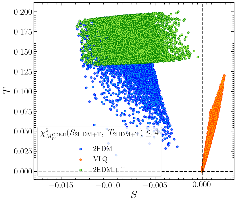
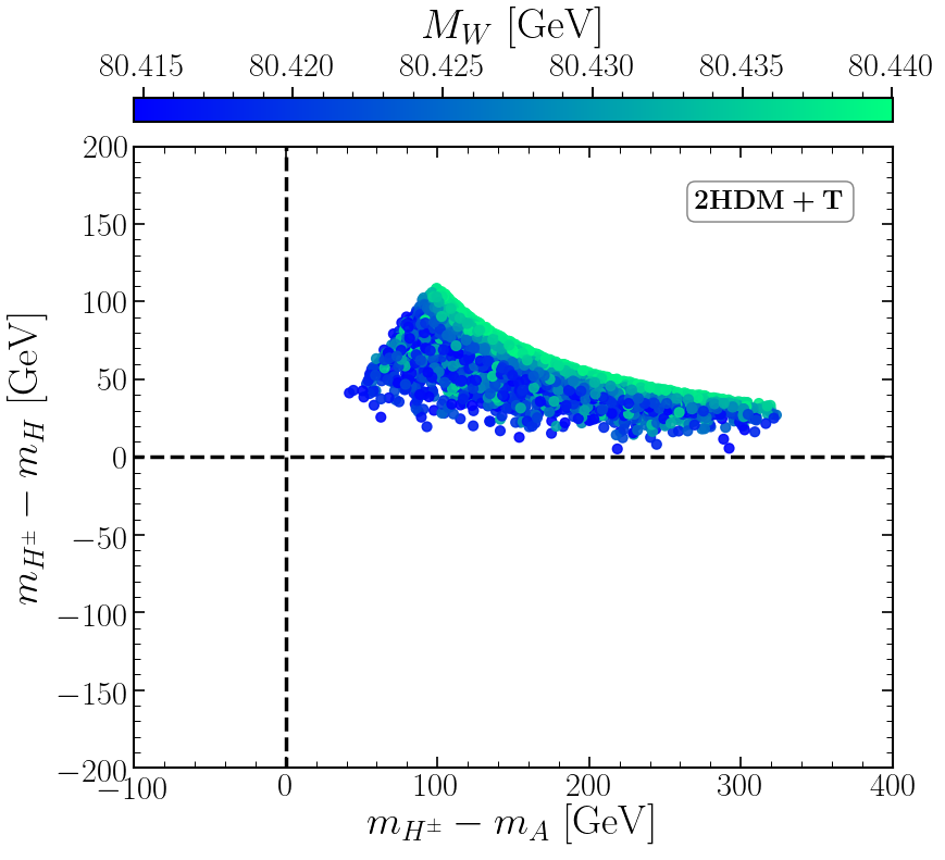
Figure 1: Left: Scan results of the 2HDM+T singlet in the $(S,~{}T)$ plane. The blue points indicate the 2HDM, while the VLQ are indicated by orange points. The combination of the 2HDM and VLQ is illustrated by green points. Right: the same data points are displayed in the $(m_{H^{\pm}}-m_{A},m_{H^{\pm}}-m_{H})$ plane, with the color code representing the value of $M_{W}$.

In Fig. 1 (left panel), we present the results of our analysis in the $(S,T)$ plane, with each contribution displayed separately. The results from the two Higgs doublet model (2HDM) are represented in blue, the VLQ in orange, and the combination of the 2HDM and VLQ are shown in green. The plot illustrates that the $T$ parameter is consistently positive for both the 2HDM and VLQ. On the other hand, the $S$ parameter is positive in the VLQ, and negative in the 2HDM. Furthermore, it is noteworthy that the cancellation between the 2HDM and VLQ leads to the $S$ parameter consistently assuming negative values in this representation. In the right panel of Fig. 1, we show the allowed parameter space in the $(m_{H^{\pm}}-m_{A},m_{H^{\pm}}-m_{H})$ plane within the 2HDM+T singlet top partner model. The color coding indicates the value of the W boson mass. One can observe that the CDF $M_{W}$ measurement value can only be reached in the case where $m_{H^{\pm}}>m_{H},m_{A}$. Like in the 2HDM, the degenerate case $m_{H^{\pm}}=m_{A}=m_{H}$ is strongly disfavored here by the CDF-II data. Morever, it can also be seen that the mass splitting between the charged Higgs boson and the CP-even Higgs $H$ can go up to 100 GeV, while the mass splitting between $H^{\pm}$ and the CP-odd Higgs boson $A$ can be at most of the order of 40 GeV to 320 GeV.

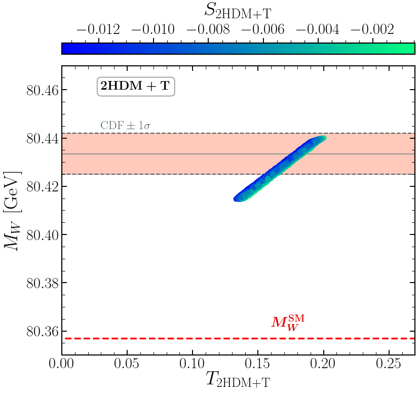
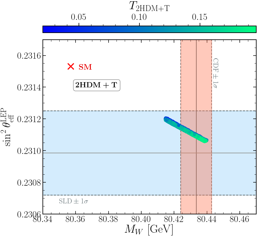
Figure 2: Scan result of the 2HDM+T singlet in the $(T,M_{W})$ plane left and $(M_{W},\sin^{2}\theta^{\mathrm{LEP}}_{\mathrm{eff}})$ right. The light red band indicates the $M_{W}$ value with the associated 1$\sigma$ uncertainty measured recently by the CDF collaboration, while the light green band shows the result of $\sin^{2}\theta_{\mathrm{eff}}$ and its associated 1$\sigma$ uncertainty measured by the SLD collaboration.

In the left panel of Fig. 2, we display the allowed parameters space of our scan with the predicted values for $M_{W}$ as a function of the $T$ parameter within the 2HDM+T singlet top partner model. The color coding of the points represents the values of the $S$ parameter. The red-dashed line shows the SM prediction for the W boson mass, and the light red region indicates the new CDF measurement at a level of $\pm 1\sigma$. It is evident from this plot that there is a positive correlation between $M_{W}^{2HDM+T}$ and the $T$ parameter as demanded by Eq. (28). The values of the $S$ parameter in the 2HDM+T singlet top partner model preferred by the CDF-II measurement of $M_{W}$ are in the range between -0.012 and -0.002. In the right panel of Fig. 2, we display the parameter points of the 2HDM+T singlet in the $(M_{W},\sin^{2}\theta^{\mathrm{LEP}}_{\mathrm{eff}})$ plane. The color coding shows the size of $T$ parameter. The light green region indicates the measurements of $\sin^{2}\theta_{\mathrm{eff}}$ within $\pm 1\sigma$ confidence level reported by the SLD collaboration, while the light red band shows the W boson mass value at $\pm 1\sigma$ recently measured by the CDF. At first sight, one can see that there is good agreement between the preferred parameter space of the CDF $M_{W}$ measurement and the value measured by the SLD experiment. Furthermore, It can be observed that there is an obvious strong negative correlation between $\sin^{2}\theta^{\mathrm{LEP}}_{\mathrm{eff}}$ and $M_{W}$ since in the $T$ parameter dominant case, a positive contribution to the W boson mass prediction corresponds to a negative contribution to the effective weak mixing angle. We find that the parameter $T$ within the 2HDM+T singlet top partner model takes values in the range between 0.05 and 0.25.

3.1.2 2HDM+B

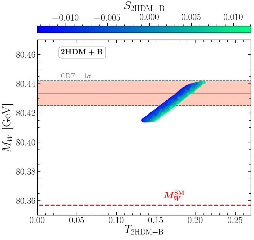
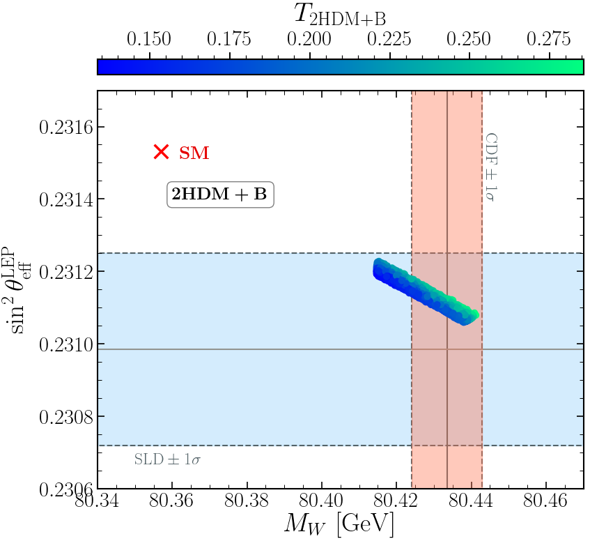
Figure 3: Scan result of the 2HDM+B singlet in the $(T,M_{W})$ plane left and $(M_{W},\sin^{2}\theta^{\mathrm{LEP}}_{\mathrm{eff}})$ right. The light red band indicates the $M_{W}$ value with the associated 1$\sigma$ uncertainty measured recently by the CDF collaboration, while the light green band shows the result of $\sin^{2}\theta_{\mathrm{eff}}$ and its associated 1$\sigma$ uncertainty measured by the SLD collaboration.

We depict the allowed parameter points in the left panel of Fig. 3. The predicted values for the W boson mass, $M_{W}$, are displayed as a function of the $T$ parameter within the 2HDM+B singlet bottom partner model. The color coding of the points represents the values of the $S$ parameter and indicates that values of S between $-0.01$ and 0.01 are preferred by the CDF’s measurement of $M_{W}$. In the right panel, we show the predictions for $M_{W}$ and $\sin^{2}\theta^{\mathrm{LEP}}_{\mathrm{eff}}$, with the color code indicating the values of the $T$ parameter. We can see that the points preferred by the CDF’s measurement of $M_{W}$ are consistent with the values of $\sin^{2}\theta^{\mathrm{LEP}}_{\mathrm{eff}}$ measured by the SLD experiment. Moreover, the $T$ parameter in the 2HDM+B singlet bottom partner model is found to be in the range between 0.14 and 0.26.

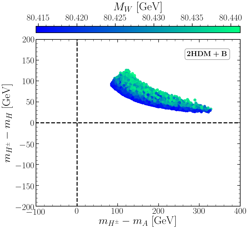
Figure 4: Scan results of the 2HDM + B singlet in the $(m_{H^{\pm}}-m_{A},m_{H^{\pm}}-m_{H})$ plane , with the colour code indicating $M_{W}$ GeV.

In Fig. 4, we plot the allowed parameter space in the $(m_{H^{\pm}}-m_{A},m_{H^{\pm}}-m_{H})$ plane in the 2HDM+B singlet bottom partner model. The color code represents the value of the W boson mass. We can see that there is only one mass hierarchy and, similarly to the behavior shown in the 2HDM+T singlet top partner model, the CDF $M_{W}$ measurement value can be explained only when $m_{H^{\pm}}>m_{H},m_{A}$. Furthermore, it can be observed that the mass splitting between the charged Higgs boson and the CP-even Higgs $H$ can be as high as 140 GeV, while the mass difference between $H^{\pm}$ and the CP-odd Higgs boson $A$ can reach 320 GeV.

3.1.3 2HDM + TB

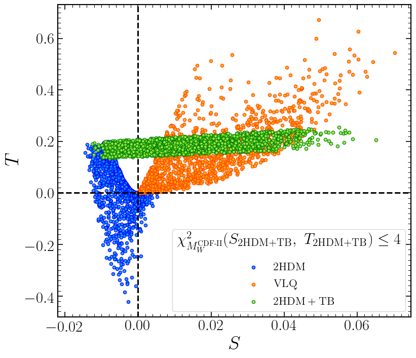
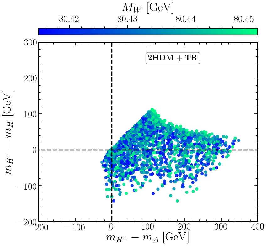
Figure 5: Left: Scan results of the 2HDM+TB doublet in the $(S,T)$ plane. The blue points indicate the 2HDM, while the VLQ are indicated by orange points. The combination of the 2HDM and VLQ is illustrated by green points. Right: the same data points are displayed in the $(m_{H^{\pm}}-m_{A},m_{H^{\pm}}-m_{H})$ plane, with the color code representing the value of $M_{W}$.

In Fig. 5 (left panel), we present the results of our analysis of the 2HDM+TB doublet scenario in the $(S,T)$ plane. The contributions of the 2HDM and the VLQs are depicted separately in blue and orange, respectively, while the combination of both models is shown in green. The plot indicates that the $T$ parameter has both positive and negative values in the 2HDM, while it is solely positive in the doublet VLQs. Similarly, the $S$ parameter displays similar behavior, with positive values in the doublet VLQs and both positive and negative values in the 2HDM. Moreover, the cancellation between the 2HDM and VLQs in this scenario results in a consistent positive value for the $T$ parameter and a combination of positive and negative values for the $S$ parameter.

In the right panel of Fig. 5, we present the allowed parameter space in the $(m_{H^{\pm}}-m_{H})$ versus $(m_{H^{\pm}}-m_{A})$ plane for the 2HDM+TB doublet. The color code represents the value of the W boson mass. It has been previously demonstrated in 2HDM studies [3] that the charged Higgs boson mass $m_{H^{\pm}}$ must be non-degenerate with the masses of the two neutral Higgs boson $m_{H}$ and $m_{A}$ in order to explain the current anomaly in the W boson mass. However, the degenerate scenario, where $m_{H^{\pm}}=m_{A}=m_{H}$, is still allowed in the 2HDM+TB top partner doublet model. Additionally, the CDF-II $M_{W}$ measurement value can also be explained in the case where $(m_{H^{\pm}}-m_{A})(m_{H^{\pm}}-m_{H})>0$ and also it is interesting to observe that the case where $m_{A}<m_{H^{\pm}}<m_{H}$ is not excluded. Note that, in the 2HDM this mass splitting region is not allowed because the $T$ parameter is negative but here the presence of the top partner doublet $TB$ pushed it to the preferred positive values required by the $M_{W}$ mass anomaly. Furthermore, we see that the mass splitting between the charged Higgs boson and the CP-odd Higgs boson can reach up to 360 GeV, while the mass difference between the charged Higgs boson and the CP-even Higgs boson $H$ can be at most 100 GeV. The large mass gap between $m_{H^{\pm}}$ and $m_{A}$ can guarantee the dominant decay mode of $H^{\pm}\rightarrow AW^{\pm}$ which is just gauge coupling and have no mixing suppression. Future experimental searches for this decay mode would be able to confirm or rule out the explanation of the recent $M_{W}$ mass anomaly within this model.

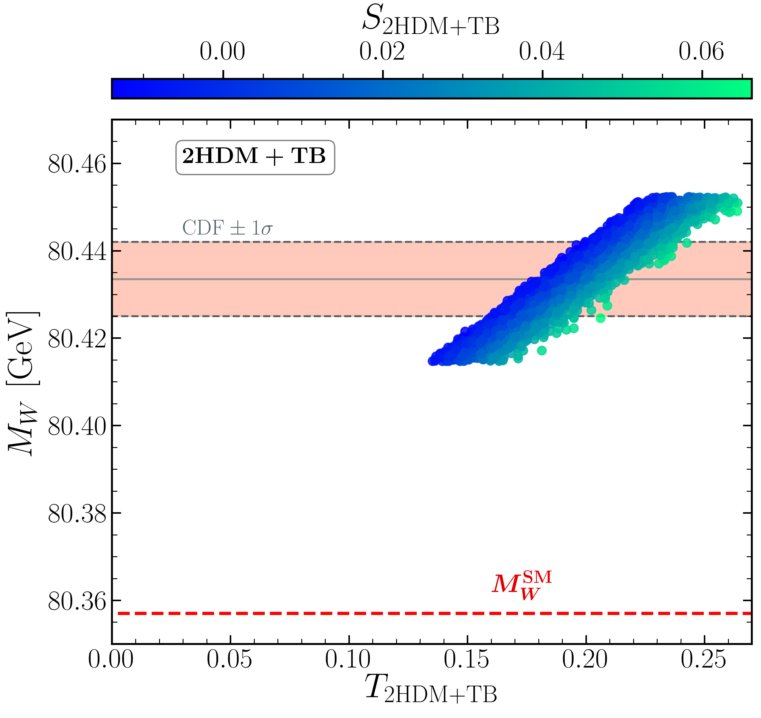
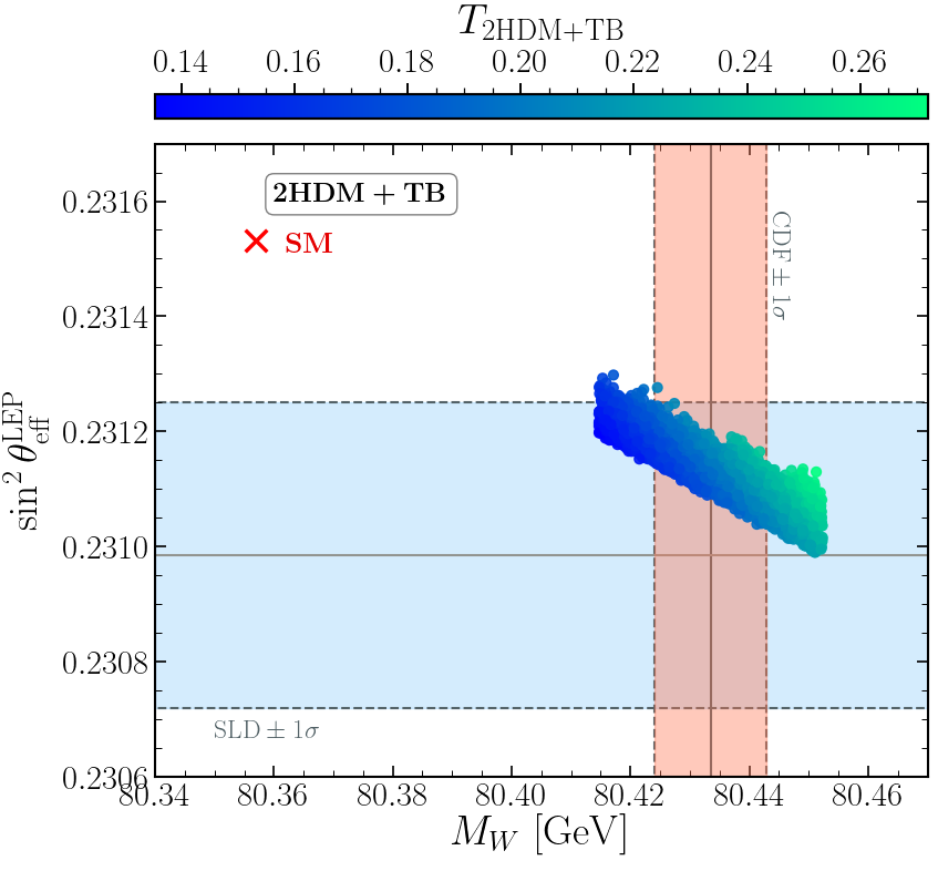
Figure 6: Scan result of the 2HDM+TB doublet in the $(T,M_{W})$ plane left and $(M_{W},\sin^{2}\theta^{\mathrm{LEP}}_{\mathrm{eff}})$ right. The light red band indicates the $M_{W}$ value with the associated 1$\sigma$ uncertainty measured recently by the CDF collaboration, while the light green band shows the result of $\sin^{2}\theta_{\mathrm{eff}}$ and its associated 1$\sigma$ uncertainty measured by the SLD collaboration.

We display in the left panel of Fig. 6 the allowed parameters points in the plane of $M_{W}$ versus $T$ within the 2HDM+TB top partner doublet model. The points are color-coded to show the values of the $S$ parameter. The red dashed line indicates the SM prediction for the W boson mass and the light red region shows the new CDF-II measurement at $\pm 1\sigma$ CL. It can seen that $M_{W}^{2HDM+TB}$ is a linear function of the $T$ parameter. Furthermore, the regions consistent with CDF-II measurement of $M_{W}$ require the values of the $S$ parameter to be in the range between 0 and 0.06. In the right panel of Fig. 6, we visualize our results within the 2HDM+TB top partner doublet model in the $\sin^{2}\theta_{\mathrm{eff}}$ versus $M_{W}$ plane. The color-coding indicates the allowed values of the $T$ parameter. It is interesting to see that full agreement is achieved between the SLD measurement of the weak mixing angle and the favored parameter space required by the CDF-II data. Also, we see that the preferred range for the $T$ parameter is almost entirely positive and varies between 0.14 and 0.26.

3.1.4 2HDM+BY or 2HDM+XT

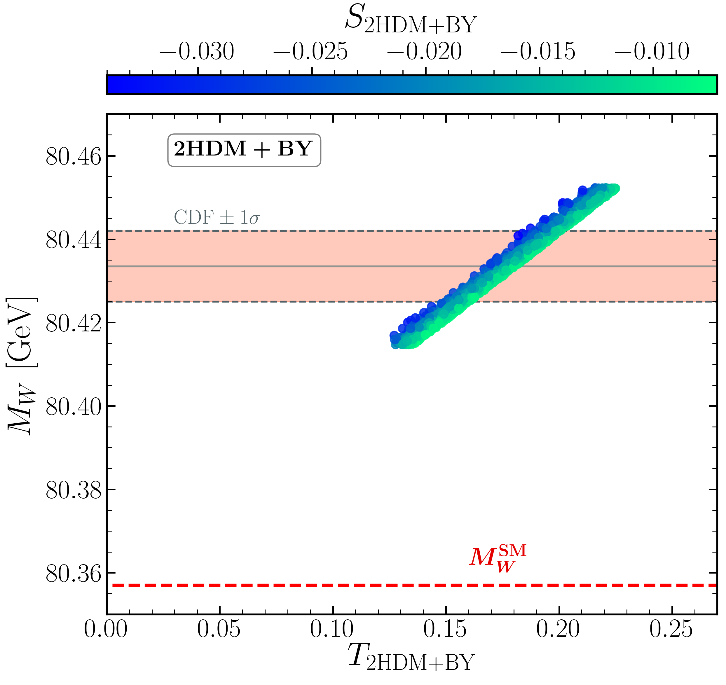
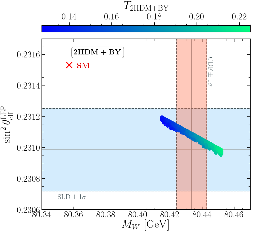
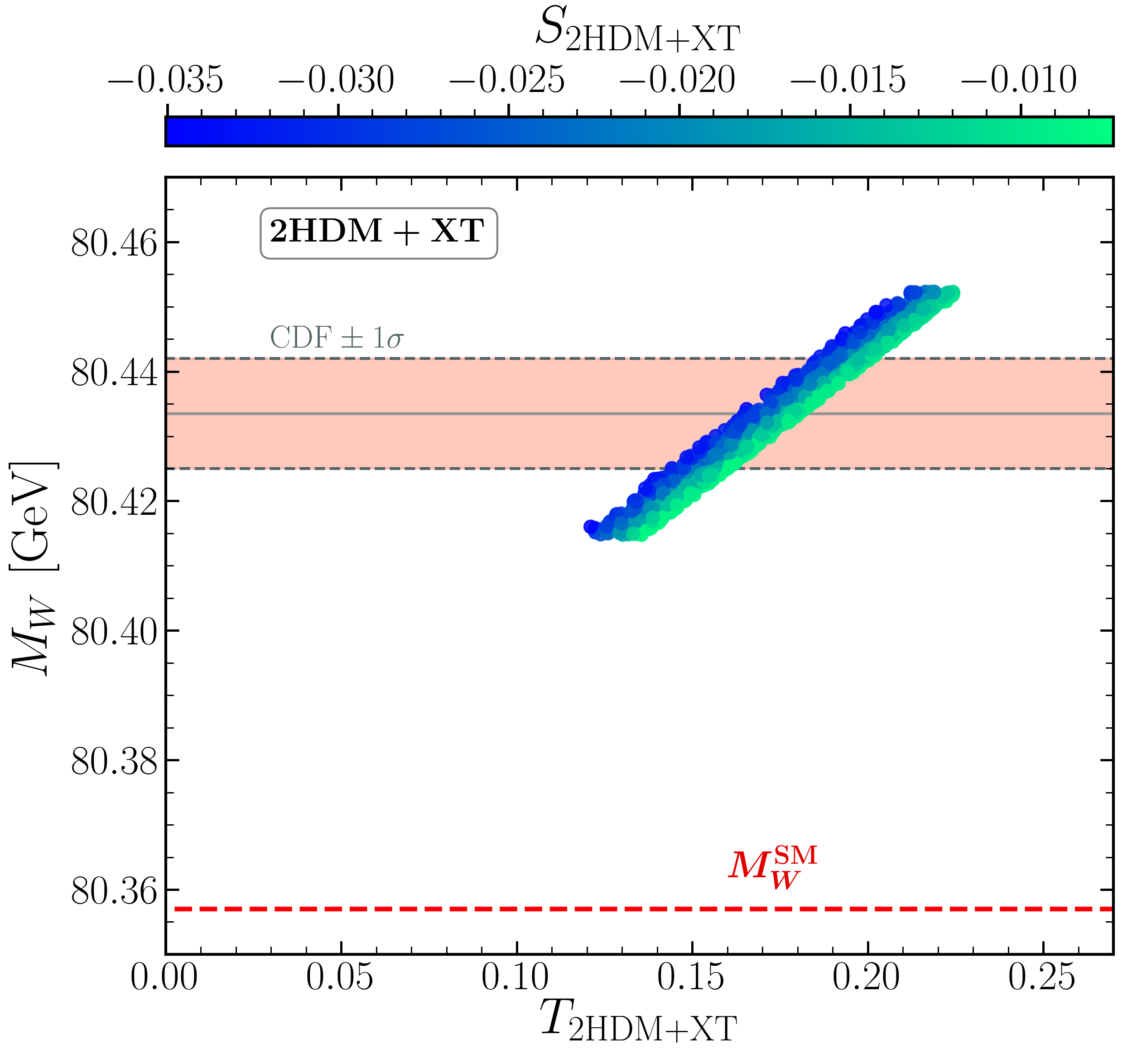
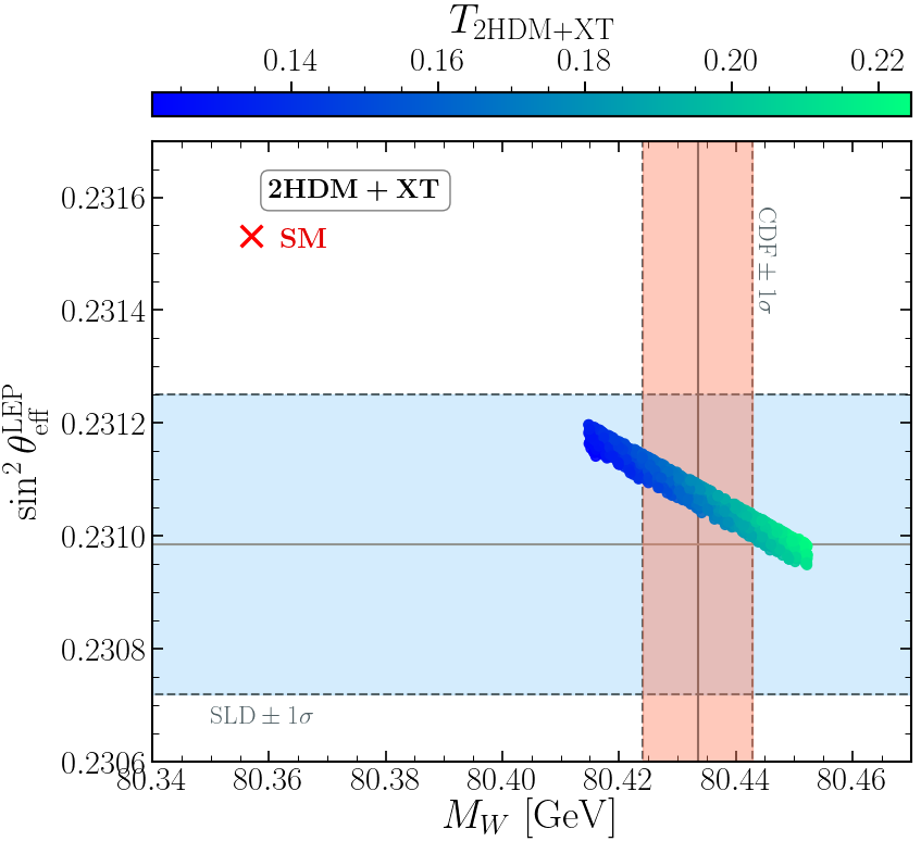
Figure 7: Scan result of the 2HDM+BY (2HDM+XT in the $T$ versus $M_{W}$ plane in the upper left panel (lower left panel) and in the $M_{W}$ versus $\sin^{2}\theta^{\mathrm{LEP}}_{\mathrm{eff}}$ plane in the upper right panel (lower right panel). The light red band indicates the $M_{W}$ value with the associated 1$\sigma$ uncertainty measured recently by the CDF collaboration, while the light green band shows the result of $\sin^{2}\theta_{\mathrm{eff}}$ and its associated 1$\sigma$ uncertainty measured by the SLD collaboration.

We display in the upper left and lower left panels of Fig. 7 the allowed parameter points in the $M_{W}$ versus $T$ plane in the frameworks of the 2HDM+BY and 2HDM+XT models, respectively. The color coding of the points shows the allowed values of $S$ parameter. The red-dashed line indicates the SM prediction for the W boson mass and the light red region displays the new CDF-II measurement at the level of $\pm 1\sigma$. One can observe that the regions consistent with CDF-II measurement of $M_{W}$ require the values of the $S$ parameter to be in the range between -0.030 and -0.01 in the 2HDM+BY model, while the favored values of the $S$ parameter in the 2HMD+XT model are still negative and range between -0.035 and -0.01. In the upper right and lower right panels of Fig. 7 we visualize our results in the $\sin^{2}\theta_{\mathrm{eff}}$ versus $M_{W}$ plane within the 2HDM+BY and 2HDM+XT models, respectively. The color code indicates the allowed values taken by the $T$ parameter. It is interesting to see that a full agreement is achieved between the weak mixing angle measured by the SLD collaboration and the favored parameters space required by the CDF-II data. Also, we see that the preferred range for the $T$ parameter for both models needed to explain the anomaly is almost entirely positive and varies between 0.14 and 0.22.

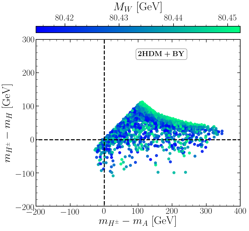
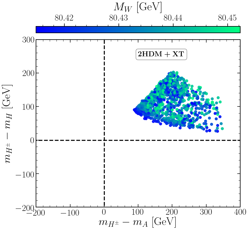
Figure 8: The points from the parameter scan of the 2HDM+BY (2HDM+XT)models in the $m_{H^{\pm}}-m_{A}$ versus $m_{H^{\pm}}-m_{H}$ plane in the left panel (right panel), with the color code indicating the W-boson mass $M_{W}$. All points have $\chi^{2}_{M_{W}^{\mathrm{CDF-II}}}\leq 4$.

In the left panel of Fig. 8, we show the allowed parameter points in the $(m_{H^{\pm}}-m_{H})$ versus $(m_{H^{\pm}}-m_{A})$ plane within the 2HDM+BY model. The color code indicates the value of the W boson mass. It is interesting to see that within this model the charged Higgs boson mass $m_{H^{\pm}}$ can be degenerate with the two neutral BSM Higgs boson masses $m_{H}$ and $m_{A}$ to accommodate the CDF-II W-boson mass. Additionally, the recent anomaly can also be explained in the case where $(m_{H^{\pm}}-m_{A})(m_{H^{\pm}}-m_{H})>0$ and again it is interesting to observe that the case where $m_{A}<m_{H^{\pm}}<m_{H}$ is not excluded due to the presence of (B,Y) doublet which gives the favored large positive values of the $T$ parameter required to accommodate the W-mass reported by the CDF-II collaboration. Furthermore, we see that the mass splitting between the charged Higgs boson and CP-odd Higgs boson can go up to 360 GeV whilst the mass splitting between $H^{\pm}$ and CP-even Higgs boson $H$ can at most be of the order of 100 GeV. In the right panel of Fig. 8 we present the allowed parameter points within the 2HDM+XT doublet model. One can observe that both splittings $m_{H^{\pm}}-m_{H}$ and $m_{H^{\pm}}-m_{A}$ are required to be simultaneously positive and always non-zero in order to be consistent with the CDF-II data. The maximum mass splitting between the charged Higgs boson and the CP-even Higgs $H$ can reach 200 GeV, while the maximum splitting between $H^{\pm}$ and the CP-odd Higgs boson $A$ can go up to 340 GeV. It should be noted that, in this model, the degenerate case where $m_{H^{\pm}}=m_{A}=m_{H}$ is ruled out by the direct Higgs boson searches at colliders, as computed by HiggsBounds-5.

3.1.5 2HDM+TBY or 2HDM+XTB

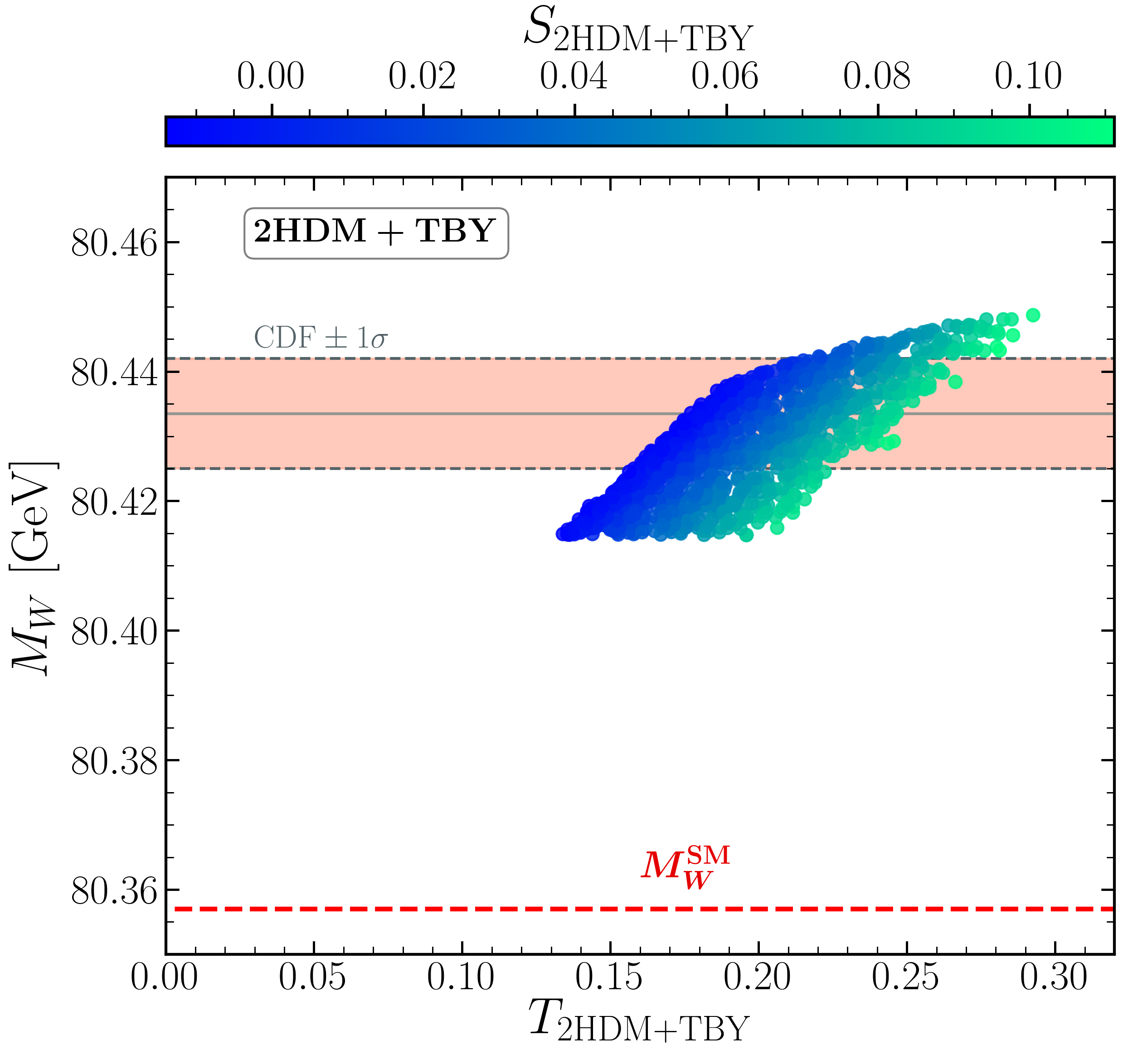
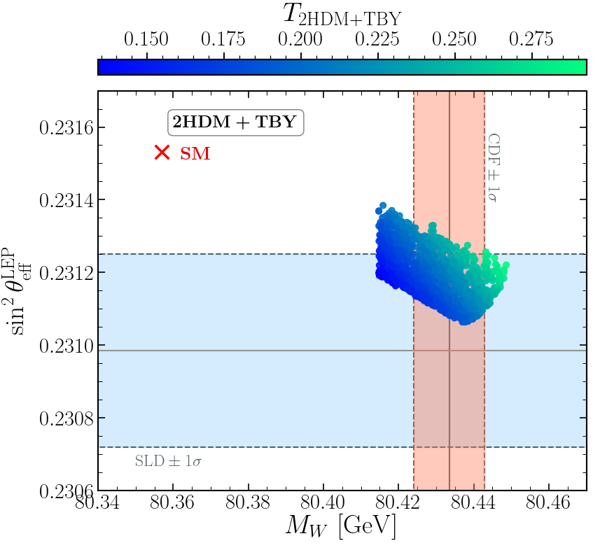
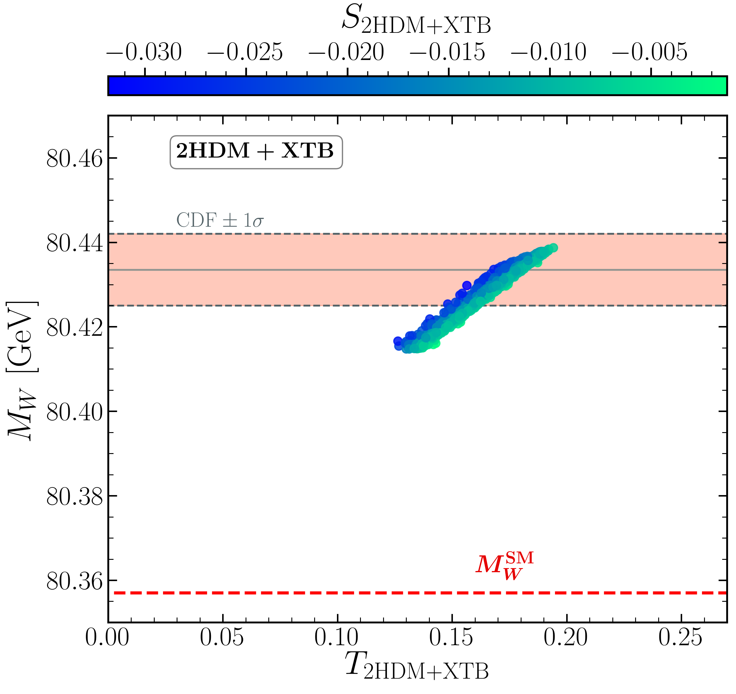
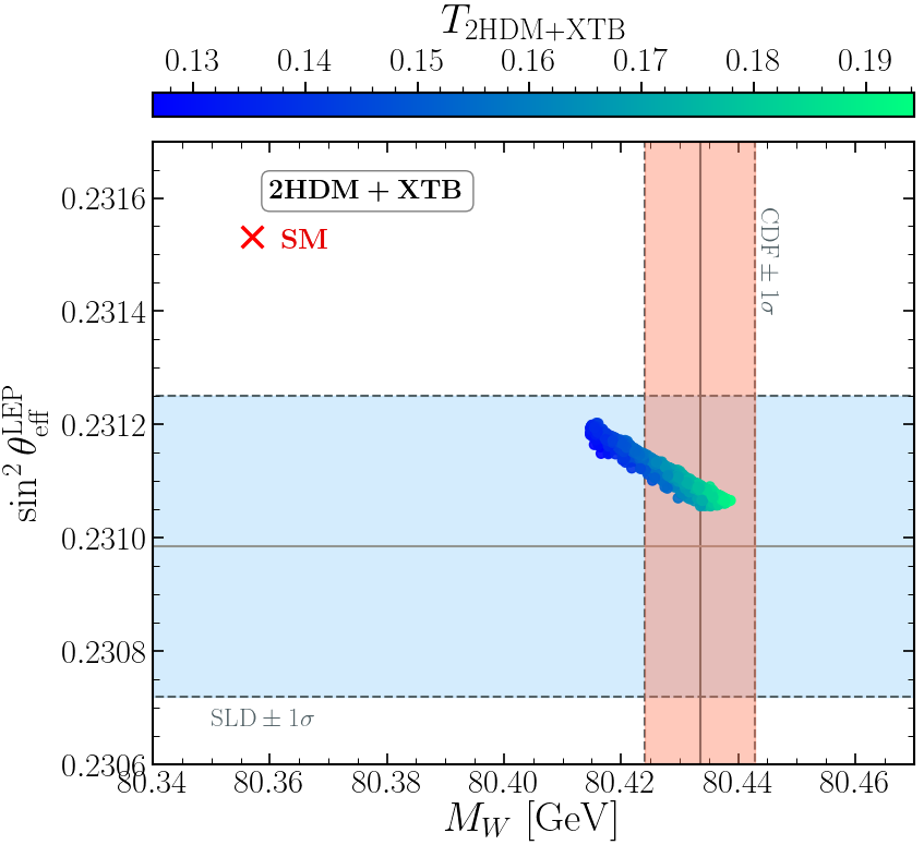
Figure 9: Scan result of the 2HDM+TBY (upper panels) and (2HDM+XTB) (lower panels) in the $T$ versus $M_{W}$ plane in the upper left panel (lower left panel) and in the $M_{W}$ versus $\sin^{2}\theta^{\mathrm{LEP}}_{\mathrm{eff}}$ plane in the upper right panel (lower right panel). The light red band indicates the $M_{W}$ value with the associated 1$\sigma$ uncertainty measured recently by the CDF collaboration, while the light green band shows the result of $\sin^{2}\theta_{\mathrm{eff}}$ and its associated 1$\sigma$ uncertainty measured by the SLD collaboration.

We present in the upper-left and lower-left panels of Fig.9 the allowed points from the parameter scan in the $M_{W}$ versus $T$ plane in the framework of the 2HDM+TBY and 2HDM+XTB triplet models, respectively. The color coding of the points indicates the allowed values of the $S$ parameter. The red-dashed line shows the SM prediction for the W-boson mass, and the light red region displays the new CDF-II measurement at the $\pm 1\sigma$ level. We can see that the regions consistent with the new CDF measurement require the values of the $S$ parameter to be in the range between -0.014 and 0.11 in the 2HDM+TBY model, while a negative $S$ parameter contribution is required to accommodate the anomaly in the 2HDM+XTB model, with favored values of the $S$ parameter ranging between -0.032 and -0.0012. In the upper-right and lower-right panels of Fig.9, we visualize, respectively, our results within the 2HDM+TBY and 2HDM+XTB models in the $\sin^{2}\theta_{\mathrm{eff}}$ versus $M_{W}$ plane. The color code indicates the allowed values taken by the $T$ parameter. Besides the fact that $M_{W}$ is anti-correlated with the weak mixing angle $\sin^{2}\theta^{\mathrm{LEP}}_{\mathrm{eff}}$, it is interesting to note that in both models there is full agreement between the weak mixing angle measured by the SLD collaboration and the points from the parameter space preferred by the CDF-II data. Also, we see that the favored range for the $T$ parameter within the 2HDM+TBY model that is required to explain the anomaly is almost entirely positive and varies between 0.13 and 0.3, while it ranges between 0.13 and 0.19 in the framework of the 2HDM+XTB model.

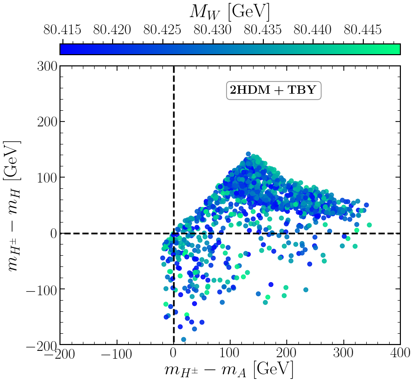
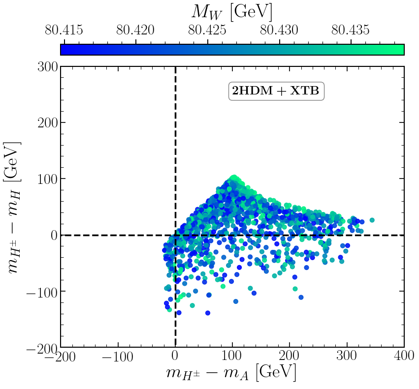
Figure 10: The points from the parameter scan of the 2HDM+TBY (2HDM+XTB) models in the $m_{H^{\pm}}-m_{A}$ versus $m_{H^{\pm}}-m_{H}$ plane in the left panel (right panel), with the color code indicating the W-boson mass $M_{W}$.

In the left panel of Fig. 10, we present the allowed parameter points in the $(m_{H^{\pm}}-m_{H})$ versus $(m_{H^{\pm}}-m_{A})$ plane within the 2HDM+TBY triplet model. The color code indicates the value of the W boson mass. At a glance, it is evident that the CDF value of $M_{W}$ can be reproduced in the scenario where the three BSM scalars are mass-degenerate, i.e., $m_{H^{\pm}}=m_{A}=m_{H}$. Additionally, the CDF-II $M_{W}$ measurement can also be explained in the case where $(m_{H^{\pm}}-m_{A})(m_{H^{\pm}}-m_{H})>0$. It is worth noting that the scenario with $m_{H}<m_{H^{\pm}}<m_{A}$ is still allowed and can accommodate the anomaly. Besides, we see that the mass splitting between the charged Higgs boson and the CP-odd Higgs can reach up to 160 GeV, while the mass splitting between $H^{\pm}$ and the CP-even Higgs $H$ can go up to 350 GeV.
In the right panel of Fig. 10, the allowed parameter space within the 2HDM+XTB model is presented. It can be seen that the degenerate scenario, in which the masses of the charged Higgs boson ($m_{H^{\pm}}$), the CP-even Higgs ($m_{H}$), and the CP-odd Higgs ($m_{A}$) are equal, cannot explain the CDF value of the W boson mass. Furthermore, it is shown that the mass difference between the charged Higgs boson and the CP-even Higgs $H$ is restricted to a range of 150 GeV to 110 GeV, while the mass difference between the charged Higgs boson and the CP-odd Higgs $A$ is limited to a range between -10 GeV and 350 GeV.

4 Conclusion

The very recent measurement result of the W-boson mass $M_{W}$ reported by the CDF collaboration deviates from the SM prediction by about 7$\sigma$. If the CDF-II result is correct, it would indicate the need for new physics beyond the Standard Model to explain the observed mass of the W boson that matches the CDF-II data. In this paper, we consider the implications of the recent W boson mass anomaly in the framework of 2HDM type II augmented by vector-like quarks. We studied all seven distinct possibilities of vector-like $SU(2)_{L}$ multiplets including singlets, doublets, and triplets. We computed the electroweak precision observables S and T using the standard scalar Passarino-Veltman functions and provided the generic analytic expressions for $S$ and $T$ and listed the couplings used for specific models such us the singlet, doublet and triplet VLQs models. In order to explain the CDF measurement we need a positive $T$ and this is possible if we consider VLQs alone, which is all time positive. In the case of the 2HDM augmented with VLQs, both $S$ and $T$ contributions are split into two separate contributions, one from VLQs and one from 2HDM which do not mix. We found that in most cases, there is a cancellation between VLQs and 2HDM contributions, which enlarges the parameter space of both models. After this observation we performed a $\chi^{2}$ analysis and found that it is possible to solve the tension between the new CDF $M_{W}$ measurement and the SM prediction. We also noticed that the scenario with 2HDM alone with a degenerate spectrum that is ruled out by the CDF measurement could survive if we include both 2HDM and VLQs. We also discussed the consequences of the 2HDM augmented with VLQs on the effective mixing angle $\sin^{2}\theta_{\text{eff}}$.

Appendix A VLQs contributions to the oblique parameters S, T and U

In this appendix we give the analytical expressions for S, T and U in the 2HDM as well as in the generic expression in the VLQ models as a function of the well-known scalar Passarino-Veltman functions.

A.1 Passarino-Veltman functions

The Passarino-Veltman functions are defined as follow:

$$A_{0}(m_{1}^{2}) = \frac{(2\pi\mu)^{4-D}}{i\pi^{2}}\int{d^{D}q\frac{1}{d_{1}}},$$ (33)

$$B_{0};B^{\mu};B^{\mu\nu}(p_{1}^{2},m_{1}^{2},m_{2}^{2}) = \frac{(2\pi\mu)^{4-D}}{i\pi^{2}}\int{d^{D}q\frac{1;q^{\mu};q^{\mu}q^{\nu}}{d_{1}d_{2}}}$$ (34)

With the denominators $d_{i}$ are defined by $d_{1}=q^{2}-m_{1}^{2}$ and $d_{2}=(q+p_{1})^{2}-m_{2}^{2}$ and $\mu$ is the renormalization scale. $p_{1}$ is the external momentum and $q$ is the internal momentum which is integrated out.

The functions $B^{\mu}$ and $B^{\mu\nu}$ can be decomposed as,

$$B^{\mu} = p_{1}^{\mu}B_{1},\quad\ B^{\mu\nu}=g^{\mu\nu}B_{00}+p_{1}^{\mu}p_{1}^{\nu}B_{11}.$$ (35)

Thus, the functions $B_{00}$ and $B_{1}$ can be calculated by contracting $B^{\mu}$ and $B^{\mu\nu}$ with $p_{1}$ and $g_{\mu\nu}$ respectively,

$$B_{1}(p^{2},m_{1}^{2},m_{2}^{2}) = \frac{1}{2}\left[A_{0}(m_{1}^{2})-A_{0}(m_{2}^{2})-\left(p^{2}+m_{1}^{2}-m_{2}^{2}\right)B_{0}(p^{2},m_{1}^{2},m_{2}^{2})\right]$$ (36)

$$B_{00}(p^{2},m_{1}^{2},m_{2}^{2}) = -\frac{p^{2}-3(m_{1}^{2}+m_{2}^{2})}{18}+\frac{m_{1}^{2}B_{0}(p^{2},m_{1}^{2},m_{2}^{2})}{3}$$ (37)

$$+\frac{A_{0}(m_{2}^{2})+(p^{2}+m_{1}^{2}-m_{2}^{2})B_{1}(p^{2},m_{1}^{2},m_{2}^{2})}{6}$$

A.2 $S$, $T$ and $U$ parameters

The oblique parameters can be parameterized in terms of the gauge bosons two-point functions as follows:

$$S = \frac{4s_{W}^{2}c_{W}^{2}}{\alpha}\Re e\Bigg{[}\frac{\Pi_{\gamma\gamma}(m_{Z}^{2})}{m_{Z}^{2}}-\frac{\Pi_{ZZ}(m_{Z}^{2})-\Pi_{ZZ}(0)}{m_{Z}^{2}}-\Big{(}\frac{c_{W}^{2}-s_{W}^{2}}{c_{W}s_{W}}\Big{)}\Big{(}\frac{\Pi_{Z\gamma}(m_{Z}^{2})+\Pi_{Z\gamma}(0)}{m_{Z}^{2}}\Big{)}\Bigg{]}$$

$$T = \frac{1}{\alpha}\Re e\left[\frac{\Pi_{ZZ}(0)}{m_{Z}^{2}}-\frac{\Pi_{WW}(0)}{m_{W}^{2}}-\frac{2s_{W}}{c_{W}}\frac{\Pi_{Z\gamma}(0)}{m_{Z}^{2}}\right]$$ (39)

$$U = \frac{4s_{W}^{2}}{\alpha}\Re e\Bigg{[}\frac{\Pi_{WW}(0)-\Pi_{WW}(m_{W}^{2})}{m_{W}^{2}}-c_{W}^{2}\frac{\Pi_{ZZ}(0)-\Pi_{ZZ}(m_{Z}^{2})}{m_{Z}^{2}}-2s_{W}c_{W}\frac{\Pi_{\gamma Z}(0)-\Pi_{\gamma Z}(m_{Z}^{2})}{m_{Z}^{2}}+$$ (40)

$$s_{W}^{2}\frac{\Pi_{\gamma\gamma}(m_{Z}^{2})}{m_{Z}^{2}}\Bigg{]}$$

Where $\alpha$ is the fine-structure constant and $c_{w}$ ($s_{w}$) denotes the cosine (sine) of the Weinberg angle.

A.3 $S$, $T$ and $U$ parameters in 2HDM

The contributions of the 2HDM to the oblique parameters S, T and U can be given as follows:

$$\Delta S = \frac{c_{W}^{2}}{\pi m_{W}^{2}}\Bigg{\{}c_{\beta-\alpha}^{2}\bigg{[}m_{Z}^{2}\Big{(}-B_{0}(0,m_{h}^{2},m_{Z}^{2})+B_{0}(m_{Z}^{2},m_{h}^{2},m_{Z}^{2})+B_{0}(0,m_{H}^{2},m_{Z}^{2})$$ (41)

$$-B_{0}(m_{Z}^{2},m_{H}^{2},m_{Z}^{2})\Big{)}+B_{00}(m_{Z}^{2},m_{h}^{2},m_{A}^{2})-B_{00}(0,m_{h}^{2},m_{A}^{2})+B_{00}(0,m_{h}^{2},m_{Z}^{2})$$

$$-B_{00}(m_{Z}^{2},m_{h}^{2},m_{Z}^{2})-B_{00}(0,m_{H}^{2},m_{Z}^{2})+B_{00}(m_{Z}^{2},m_{H}^{2},m_{Z}^{2})\bigg{]}$$

$$+s_{\beta-\alpha}^{2}\bigg{[}B_{00}(m_{Z}^{2},m_{H}^{2},m_{A}^{2})-B_{00}(0,m_{H}^{2},m_{A}^{2})\bigg{]}-B_{00}(m_{Z}^{2},m_{H^{\pm}}^{2},m_{H^{\pm}}^{2})$$

$$+(c_{W}^{2}-s_{W}^{2})^{2}B_{00}(0,m_{H^{\pm}}^{2},m_{H^{\pm}}^{2})+2A_{0}(m_{H^{\pm}}^{2})s_{W}^{2}c_{W}^{2}\Bigg{\}}$$

$$\Delta T= \frac{1}{4m_{W}^{2}\pi s_{W}^{2}}\Big{\{}m_{W}^{2}c^{2}_{\beta-\alpha}B_{0}(0,m_{h}^{2},m_{W}^{2})+s^{2}_{\beta-\alpha}B_{00}(0,m_{h}^{2},m_{W}^{2})$$

$$-c^{2}_{\beta-\alpha}\left[m_{Z}^{2}B_{0}(0,m_{h}^{2},m_{Z}^{2})-B_{00}(0,m_{h}^{2},m_{Z}^{2})\right]$$

$$-c^{2}_{\beta-\alpha}\left[m_{W}^{2}B_{0}(0,m_{H}^{2},m_{W}^{2})-B_{00}(0,m_{H}^{2},m_{W}^{2})\right]+c^{2}_{\beta-\alpha}\left[m_{Z}^{2}B_{0}(0,m_{H}^{2},m_{Z}^{2})-B_{00}(0,m_{H}^{2},m_{Z}^{2})\right]$$

$$-2m_{H^{\pm}}^{2}s_{W}^{4}B_{0}(0,m_{H^{\pm}}^{2},m_{H^{\pm}}^{2})+(4s_{W}^{4}-1)B_{00}(0,m_{H^{\pm}}^{2},m_{H^{\pm}}^{2})$$

$$-c^{2}_{\beta-\alpha}\left[B_{00}(0,m_{h}^{2},m_{A}^{2})-B_{00}(0,m_{h}^{2},m_{H^{\pm}}^{2})\right]$$

$$-s^{2}_{\beta-\alpha}\left[B_{00}(0,m_{H}^{2},m_{A}^{2})-B_{00}(0,m_{H}^{2},m_{H^{\pm}}^{2})\right]+B_{00}(0,m_{A}^{2},m_{H^{\pm}}^{2})-B_{00}(0,m_{W}^{2},m_{h}^{2})$$

$$-B_{00}(0,m_{W}^{2},m_{Z}^{2})+B_{00}(0,m_{Z}^{2},m_{W}^{2})-2m_{H^{\pm}}^{2}s_{W}^{4}\Big{\}}$$ (42)

$$\Delta U = \frac{1}{\pi m_{W}^{2}}\Bigg{\{}c_{\beta-\alpha}\Big{[}m_{Z}^{2}c_{W}^{2}B_{0}(0,m_{h}^{2},m_{Z}^{2})-m_{Z}^{2}c_{W}^{2}B_{0}(0,m_{h}^{2},m_{W}^{2})$$ (43)

$$-m_{Z}^{2}c_{W}^{2}B_{0}(m_{Z}^{2},m_{h}^{2},m_{Z}^{2})+m_{Z}^{2}c_{W}^{2}B_{0}(m_{W}^{2},m_{h}^{2},m_{W}^{2})-m_{Z}^{2}c_{W}^{2}B_{0}(0,m_{H}^{2},m_{Z}^{2})$$

$$+m_{Z}^{2}c_{W}^{2}B_{0}(0,m_{H}^{2},m_{W}^{2})+m_{Z}^{2}c_{W}^{2}B_{0}(m_{Z}^{2},m_{H}^{2},m_{Z}^{2})-m_{Z}^{2}c_{W}^{2}B_{0}(m_{W}^{2},m_{H}^{2},m_{W}^{2})$$

$$-c_{W}^{2}B_{00}(m_{Z}^{2},m_{h}^{2},m_{A}^{2})+c_{W}^{2}B_{00}(0,m_{h}^{2},m_{A}^{2})-c_{W}^{2}B_{00}(0,m_{h}^{2},m_{Z}^{2})$$

$$+c_{W}^{2}B_{00}(m_{Z}^{2},m_{h}^{2},m_{Z}^{2})+c_{W}^{2}B_{00}(0,m_{H}^{2},m_{Z}^{2})-c_{W}^{2}B_{00}(m_{Z}^{2},m_{H}^{2},m_{Z}^{2})$$

$$+B_{00}(m_{W}^{2},m_{h}^{2},m_{H^{\pm}}^{2})-B_{00}(0,m_{h}^{2},m_{H^{\pm}}^{2})-B_{00}(0,m_{H}^{2},m_{W}^{2})$$

$$+B_{00}(m_{W}^{2},m_{H}^{2},m_{W}^{2})\Big{]}-s_{\beta-\alpha}\Big{[}c_{W}^{2}B_{00}(m_{Z}^{2},m_{H}^{2},m_{A}^{2})+c_{W}^{2}B_{00}(0,m_{H}^{2},m_{A}^{2})$$

$$-B_{00}(0,m_{h}^{2},m_{W}^{2})+B_{00}(m_{W}^{2},m_{h}^{2},m_{W}^{2})+B_{00}(m_{W}^{2},m_{H}^{2},m_{H^{\pm}}^{2})-B_{00}(0,m_{H}^{2},m_{H^{\pm}}^{2})\Big{]}$$

$$+B_{00}(m_{W}^{2},m_{A}^{2},m_{H^{\pm}}^{2})-B_{00}(0,m_{A}^{2},m_{H^{\pm}}^{2})+B_{00}(0,m_{W}^{2},m_{h}^{2})-B_{00}(m_{W}^{2},m_{W}^{2},m_{h}^{2})$$

$$-c_{W}^{2}B_{00}(m_{Z}^{2},m_{H^{\pm}}^{2},m_{H^{\pm}}^{2})-\frac{1}{2}c_{W}^{2}(-4c_{2W}+c_{4W}+1)B_{00}(0,m_{H^{\pm}}^{2},m_{H^{\pm}}^{2})-B_{00}(0,m_{Z}^{2},m_{W}^{2})$$

$$+B_{00}(0,m_{W}^{2},m_{Z}^{2})+B_{00}(m_{W}^{2},m_{Z}^{2},m_{W}^{2})-B_{00}(m_{W}^{2},m_{W}^{2},m_{Z}^{2})+2A_{0}(m_{H^{\pm}}^{2})s_{W}^{4}c_{W}^{2}\Bigg{\}}$$

It is understood that in the above expressions for $\Delta S$, $\Delta T$, and $\Delta U$, the SM bosonic contribution has been subtracted from the 2HDM contribution.

A.4 $S$, $T$ and $U$ parameters in VLQs

We use FeynArts/FormCalc public codes to calculate the analytical expressions of the self-energy of the gauge bosons, presented in equations (LABEL:eq:S_expression) and (39), in a scenario where VLQs interact only with third generation SM quarks. By taking into account only the contribution of those heavy quarks (both SM top and bottom as well as the new VLQs) to the self-energy, as the other contributions are the same as in the SM, the expressions of the electroweak gauge boson self-energies can be written as:

$$-\Pi_{\gamma Z}(q^{2}) = \sum_{f}{g_{\gamma z}(c_{Zff}^{L},c_{Zff}^{R},Q_{f},m_{f}^{2},q^{2})}$$ (44)

$$-\Pi_{\gamma\gamma}(q^{2}) = \sum_{f}{g_{vv}(Q_{f},Q_{f},m_{f}^{2},m_{f}^{2},q^{2})}$$ (45)

$$-\Pi_{ZZ}(q^{2}) = 2\sum_{f_{i}\neq f_{j}}{\delta_{0}{(|Q_{f_{i}}-Q_{f_{j}}|)}g_{vv}\left(c_{Zf_{i}f_{j}}^{L},c_{Zf_{i}f_{j}}^{R},m_{f_{i}}^{2},m_{f_{j}}^{2},q^{2}\right)}$$ (46)

$$+\sum_{f}{g_{vv}\left(c_{Zff}^{L},c_{Zff}^{R},m_{f}^{2},m_{f}^{2},q^{2}\right)}$$

$$-\Pi_{WW}(q^{2}) = \sum_{f_{i}\neq f_{j}}{\delta_{1}{(|Q_{f_{i}}-Q_{f_{j}}|)}g_{vv}\left(c_{Wf_{i}f_{j}}^{L},c_{Wf_{i}f_{j}}^{R},m_{f_{i}}^{2},m_{f_{j}}^{2},q^{2}\right)}$$ (47)

Where $c_{Vff}$ are the couplings between the gauge boson Z or W and two fermions ($f=t,b,T,X,B,Y$) given in App. B , $\delta_{d}$ is the Dirac function with a non-null value at d, and the functions $g_{ab}$ are defined as,

$g_{vv}$ and $g_{Z\gamma}$ are given by:

$$g_{vv}\left(x,y,m_{1}^{2},m_{2}^{2},k^{2}\right) = \frac{N_{c}}{8\pi^{2}}\Big{[}(x^{2}+y^{2})\big{(}A_{0}(m_{2}^{2})-2B_{00}(k^{2},m_{1}^{2},m_{2}^{2})+k^{2}B_{1}(k^{2},m_{1}^{2},m_{2}^{2})\big{)}$$ (48)

$$+\big{(}(x^{2}+y^{2})m_{1}^{2}-2xym_{1}m_{2}\big{)}B_{0}(k^{2},m_{1}^{2},m_{2}^{2})\Big{]}$$

$$g_{\gamma z}\left(x,y,Q,m^{2},k^{2}\right) = \frac{-N_{c}}{8\pi^{2}}\Big{[}(x+y)Q\big{(}A_{0}(m^{2})-2B_{00}(k^{2},m^{2},m^{2})$$ (49)

$$+k^{2}B_{1}(k^{2},m^{2},m^{2})\big{)}\Big{]}$$

Where the $N_{c}$ is the color factor with $N_{c}=3$ for quarks. $A_{0}$, $B_{0}$, $B_{00}$ and $B_{1}$ are the usual Passarino-Veltman functions.

The SM contribution to S and T is calculated by considering the exchange of only top and bottom quarks in the self-energies of the gauge bosons, and the SM couplings used are given by Eq.(67).

After computing the expressions of the $S$, $T$ and $U$ parameters for both the SM and the SM augmented with VLQs, it is necessary to perform a subtraction to extract the contribution of new physics to the oblique parameters.

$$\Delta S=S_{SM+VLQs}-S_{SM},\ \Delta T=T_{SM+VLQs}-T_{SM},\ \Delta U=U_{SM+VLQs}-U_{SM}$$ (50)

It is important to note that we checked that both S, T and U are UV finite and renormalization scale $\mu$ independent in all the aforementioned models.

The oblique parameters of the extensions with VLQs have been studied in many works [19, 6, 17, 16]. In our analysis, we have compared our results numerically with some of those papers and found the following conclusions:

• Our expressions for the oblique parameter $T$ are in agreement with all the previously mentioned papers in all extensions, except in the SM+XTB case where there is a disagreement with those of the Ref. [17].

• The approximation proposed in Eqs.(25),(26),(27), and (28) of [16] can lead to large deviations in the evaluation of the oblique parameter $S$ in the SM +$B$, $XT$, $BY$ extension, but when using the general terms proposed in Eqs. (17), (18), (22), and (23) of [16], these deviations disappear in the case of large $s^{d}_{R}$ in the SM +$TB$ extension.

• The expression for the $S$ parameter in the triplet extensions cannot be obtained in the same manner as in [17] where they extended the formulations from Ref.[16] to calculate this oblique parameter. This can be problematic, as demonstrated in Ref.[18].

Appendix B Gauge interactions of the vector-like quarks

The neutral and charged currents are modified by the presence of VLQs, the couplings between the exotic heavy quarks to the SM third generation quarks and the electroweak massive gauge bosons can be parametrized as follows:

$$Zq^{\prime}q = \frac{e}{2s_{w}c_{w}}\gamma^{\mu}(\lambda^{L}_{Zq^{\prime}q}\mathbb{L}+\lambda^{R}_{Zq^{\prime}q}\mathbb{R}),$$

$$Wq^{\prime}q = \frac{e}{\sqrt{2}s_{w}}\gamma^{\mu}(\lambda^{L}_{Wq^{\prime}q}\mathbb{L}+\lambda^{R}_{Wq^{\prime}q}\mathbb{R})$$ (51)

Where $\lambda_{Vq^{\prime}q}^{L,R}$ are the components for both left- and right-handed couplings of the Z and W bosons. Note that these couplings depend on the chosen representations of VLQs as follows:

B.1 Vector-like singlet T

In the $SU(2)_{L}$ vector-like singlet T scenario, the left and right handed charged current couplings $\lambda_{Wq^{\prime}q}^{L,R}$ are given by:

$$\lambda_{Wtb}^{L} = c_{L}^{u},\quad\lambda_{Wtb}^{R}=0,$$

$$\lambda_{WTb}^{L} = s_{L}^{u},\quad\lambda_{WTb}^{R}=0.$$ (52)

the left and right handed neutral current couplings $\lambda^{L,R}_{Zq^{\prime}q}$ are given by:

$$\lambda_{Ztt}^{L} = (c_{L}^{u})^{2}-\frac{4}{3}s_{W}^{2},\quad\lambda_{Ztt}^{R}=-\frac{4}{3}s_{W}^{2},$$

$$\lambda_{Zbb}^{L} = -1+\frac{2}{3}s_{W}^{2},\quad\lambda_{Zbb}^{R}=\frac{2}{3}s_{W}^{2},$$

$$\lambda_{ZTT}^{L} = (s_{L}^{u})^{2}-\frac{4}{3}s_{W}^{2},\quad\lambda_{ZTT}^{R}=-\frac{4}{3}s_{W}^{2},$$

$$\lambda_{ZtT}^{L} = s_{L}^{u}c_{L}^{u},\quad\lambda_{ZtT}^{R}=0.$$ (53)

B.2 Vector-like singlet B

In the $SU(2)_{L}$ vector-like B singlet scenario, the left and right-handed quarks-W boson couplings $\lambda_{Wq^{\prime}q}^{L,R}$ are given by:

$$\lambda_{Wtb}^{L} = c_{L}^{d},\quad\lambda_{Wtb}^{R}=0,$$

$$\lambda_{WtB}^{L} = s_{L}^{d}\ ,\quad\lambda_{WtB}^{R}=0.$$ (54)

While the neutral current couplings to the Z boson are given by:

$$\lambda_{Ztt}^{L} = 1-\frac{4}{3}s_{W}^{2},\quad\lambda_{Ztt}^{R}=-\frac{4}{3}s_{W}^{2},$$

$$\lambda_{Zbb}^{L} = -(c_{L}^{d})^{2}+\frac{2}{3}s_{W}^{2},\quad\lambda_{Zbb}^{R}=\frac{2}{3}s_{W}^{2},$$

$$\lambda_{ZBB}^{L} = -(s_{L}^{d})^{2}+\frac{2}{3}s_{W}^{2},\quad\lambda_{ZBB}^{R}=\frac{2}{3}s_{W}^{2},$$

$$\lambda_{ZbB}^{L} = -s_{L}^{d}c_{L}^{d},\quad\lambda_{ZbB}^{R}=0.$$ (55)

B.3 Vector-like doublet TB

In the case of the $TB$ doublet model, the couplings between T , B and the SM third generation quarks with the W-boson are given by:

$$\lambda_{Wtb}^{L} = c_{L}^{u}c_{L}^{d}+s_{L}^{u}s_{L}^{d},\quad\lambda_{Wtb}^{R}=s_{R}^{u}s_{R}^{d},$$

$$\lambda_{WTB}^{L} = c_{L}^{u}c_{L}^{d}+s_{L}^{u}s_{L}^{d},\quad\lambda_{WTB}^{R}=c_{R}^{u}c_{R}^{d},$$

$$\lambda_{WTb}^{L} = s_{L}^{u}c_{L}^{d}-c_{L}^{u}s_{L}^{d},\quad\lambda_{WTb}^{R}=-c_{R}^{u}s_{R}^{d},$$

$$\lambda_{WtB}^{L} = c_{L}^{u}s_{L}^{d}-s_{L}^{u}c_{L}^{d},\quad\lambda_{WtB}^{R}=-s_{R}^{u}c_{R}^{d}.$$ (56)

The left and right-handed neutral current couplings to the Z boson are given by:

$$\lambda_{Ztt}^{L} = 1-\frac{4}{3}s_{W}^{2},\quad\lambda_{Ztt}^{R}=(s_{R}^{u})^{2}-\frac{4}{3}s_{W}^{2},$$

$$\lambda_{Zbb}^{L} = -1+\frac{2}{3}s_{W}^{2},\quad\lambda_{Zbb}^{R}=-(s_{R}^{d})^{2}+\frac{2}{3}s_{W}^{2},$$

$$\lambda_{ZTT}^{L} = 1-\frac{4}{3}s_{W}^{2},\quad\lambda_{ZTT}^{R}=(c_{R}^{u})^{2}-\frac{4}{3}s_{W}^{2},$$

$$\lambda_{ZBB}^{L} = -1+\frac{2}{3}s_{W}^{2},\quad\lambda_{ZBB}^{R}=-(c_{R}^{d})^{2}+\frac{2}{3}s_{W}^{2},$$

$$\lambda_{ZtT}^{L} = 0,\quad\quad\lambda_{ZtT}^{R}=-s_{R}^{u}c_{R}^{u},$$

$$\lambda_{ZbB}^{L} = 0,\quad\quad\lambda_{ZbB}^{R}=s_{R}^{d}c_{R}^{d}.$$ (57)

B.4 Vector-like doublet XT

For the XT doublet model, the couplings between the X and T heavy quarks and the third generation SM quarks with the W boson are defined as:

$$\lambda_{Wtb}^{L} = c_{L}^{u},\quad\lambda_{Wtb}^{R}=0,$$

$$\lambda_{WTb}^{L} = s_{L}^{u},\quad\lambda_{WTb}^{R}=0,$$

$$\lambda_{WtX}^{L} = -s_{L}^{u},\quad\lambda_{WtX}^{R}=-s_{R}^{u},$$

$$\lambda_{WXT}^{L} = c_{L}^{u},\quad\lambda_{WXT}^{R}=c_{R}^{u}.$$ (58)

the left- and right-handed neutral current couplings to the Z boson $\lambda^{L,R}_{Zq^{\prime}q}$ are defined as:

$$\lambda_{Ztt}^{L} = 1-2(s_{L}^{u})^{2}-\frac{4}{3}s_{W}^{2},\quad\lambda_{Ztt}^{R}=-(s_{R}^{u})^{2}-\frac{4}{3}s_{W}^{2},$$

$$\lambda_{Zbb}^{L} = -1+\frac{2}{3}s_{W}^{2},\quad\lambda_{Zbb}^{R}=\frac{2}{3}s_{W}^{2},$$

$$\lambda_{ZTT}^{L} = 1-2(c_{L}^{u})^{2}-\frac{4}{3}s_{W}^{2},\quad\lambda_{ZTT}^{R}=-(c_{R}^{u})^{2}-\frac{4}{3}s_{W}^{2},$$

$$\lambda_{ZXX}^{L} = 1-\frac{10}{3}s_{W}^{2},\quad\lambda_{ZXX}^{R}=1-\frac{10}{3}s_{W}^{2},$$

$$\lambda_{ZtT}^{L} = 2s_{L}^{u}c_{L}^{u},\quad\lambda_{ZtT}^{R}=c_{R}^{u}s_{R}^{u}.$$ (59)

B.5 Vector-like doublet BY

In the case of the BY doublet model, the interaction of vector-like B and Y quarks and the third generation SM quarks with the W boson are defined as:

$$\lambda_{Wtb}^{L} = c_{L}^{d},\quad\lambda_{Wtb}^{R}=0,$$

$$\lambda_{WtB}^{L} = s_{L}^{d},\quad\lambda_{WtB}^{R}=0,$$

$$\lambda_{WbY}^{L} = -s_{L}^{d},\quad\lambda_{WbY}^{R}=-s_{R}^{d},$$

$$\lambda_{WBY}^{L} = c_{L}^{d},\quad\lambda_{WBY}^{R}=c_{R}^{d}.$$ (60)

The neutral current couplings to the Z boson for both the left- and right-handed states are given by:

$$\lambda_{Ztt}^{L} = 1-\frac{4}{3}s_{W}^{2},\quad\lambda_{Ztt}^{R}=-\frac{4}{3}s_{W}^{2},$$

$$\lambda_{Zbb}^{L} = -1+2(s_{L}^{d})^{2}+\frac{2}{3}s_{W}^{2},\quad\lambda_{Zbb}^{R}=(s_{R}^{d})^{2}+\frac{2}{3}s_{W}^{2},$$

$$\lambda_{ZBB}^{L} = -1+2(c_{L}^{d})^{2}+\frac{2}{3}s_{W}^{2},\quad\lambda_{ZBB}^{R}=(c_{R}^{d})^{2}+\frac{2}{3}s_{W}^{2},$$

$$\lambda_{ZYY}^{L} = -1+\frac{8}{3}s_{W}^{2},\quad\lambda_{ZYY}^{R}=-1+\frac{8}{3}s_{W}^{2},$$

$$\lambda_{ZbB}^{L} = -2s_{L}^{d}c_{L}^{d},\quad\quad\lambda_{ZbB}^{R}=-s_{R}^{d}c_{R}^{d}.$$ (61)

B.6 Vector-like triplet XTB

In the framework of the XTB triplet model, the left- and right-handed charged current couplings $\lambda_{Wq^{\prime}q}^{L,R}$ are expressed as follows:

$$\lambda_{Wtb}^{L} = c_{L}^{u}c_{L}^{d}+\sqrt{2}s_{L}^{u}s_{L}^{d},\quad\lambda_{Wtb}^{R}=\sqrt{2}s_{R}^{u}s_{R}^{d},$$

$$\lambda_{WTB}^{L} = s_{L}^{u}s_{L}^{d}+\sqrt{2}c_{L}^{u}c_{L}^{d},\quad\lambda_{WTB}^{R}=\sqrt{2}c_{R}^{u}c_{R}^{d},$$

$$\lambda_{WtB}^{L} = c_{L}^{u}s_{L}^{d}-\sqrt{2}s_{L}^{u}c_{L}^{d},\quad\lambda_{WtB}^{R}=-\sqrt{2}s_{R}^{u}c_{R}^{d},$$

$$\lambda_{WTb}^{L} = s_{L}^{u}c_{L}^{d}-\sqrt{2}c_{L}^{u}s_{L}^{d},\quad\lambda_{WTb}^{R}=-\sqrt{2}c_{R}^{u}s_{R}^{d},$$

$$\lambda_{WtX}^{L} = -\sqrt{2}s_{L}^{u},\quad\lambda_{WtX}^{R}=-\sqrt{2}s_{R}^{u},$$

$$\lambda_{WXT}^{L} = \sqrt{2}c_{L}^{u},\quad\lambda_{WXT}^{R}=\sqrt{2}c_{R}^{u}.$$ (62)

While, the left- and right-handed neutral current couplings $\lambda^{L,R}_{Zf^{\prime}f}$ are defined as

$$\lambda_{Ztt}^{L} = (c_{L}^{u})^{2}-\frac{4}{3}s_{W}^{2},\quad\lambda_{Ztt}^{R}=-\frac{4}{3}s_{W}^{2},$$

$$\lambda_{Zbb}^{L} = -1-(s_{L}^{d})^{2}+\frac{2}{3}s_{W}^{2},\quad\lambda_{Zbb}^{R}=-2(s_{R}^{d})^{2}+\frac{2}{3}s_{W}^{2},$$

$$\lambda_{ZTT}^{L} = (s_{L}^{u})^{2}-\frac{4}{3}s_{W}^{2},\quad\lambda_{ZTT}^{R}=-\frac{4}{3}s_{W}^{2},$$

$$\lambda_{ZBB}^{L} = -1-(c_{L}^{d})^{2}+\frac{2}{3}s_{W}^{2},\quad\lambda_{ZBB}^{R}=-2(c_{R}^{d})^{2}+\frac{2}{3}s_{W}^{2},$$

$$\lambda_{ZXX}^{L} = 2-+\frac{10}{3}s_{W}^{2},\quad\lambda_{ZXX}^{R}=2-+\frac{10}{3}s_{W}^{2},$$

$$\lambda_{ZtT}^{L} = s_{L}^{u}c_{L}^{u},\quad\quad\lambda_{ZtT}^{R}=0,$$

$$\lambda_{ZbB}^{L} = s_{L}^{d}c_{L}^{d},\quad\quad\lambda_{ZbB}^{R}=2s_{R}^{d}c_{R}^{d}.$$ (63)

B.7 Vector-like triplet TBY

In the TBY triplet model, the interactions between the vector-like T, B, and Y quarks, as well as the third generation SM quarks, with the W boson are defined as:

$$\lambda_{Wtb}^{L} = c_{L}^{u}c_{L}^{d}+\sqrt{2}s_{L}^{u}s_{L}^{d},\quad\lambda_{Wtb}^{R}=\sqrt{2}s_{R}^{u}s_{R}^{d},$$

$$\lambda_{WTB}^{L} = s_{L}^{u}s_{L}^{d}+\sqrt{2}c_{L}^{u}c_{L}^{d},\quad\lambda_{WTB}^{R}=\sqrt{2}c_{R}^{u}c_{R}^{d},$$

$$\lambda_{WtB}^{L} = c_{L}^{u}s_{L}^{d}-\sqrt{2}s_{L}^{u}c_{L}^{d},\quad\lambda_{WtB}^{R}=-\sqrt{2}s_{R}^{u}c_{R}^{d},$$

$$\lambda_{WTb}^{L} = s_{L}^{u}c_{L}^{d}-\sqrt{2}c_{L}^{u}s_{L}^{d},\quad\lambda_{WTb}^{R}=-\sqrt{2}c_{R}^{u}s_{R}^{d},$$

$$\lambda_{WbY}^{L} = -\sqrt{2}s_{L}^{d},\quad\lambda_{WbY}^{R}=-\sqrt{2}s_{R}^{d},$$

$$\lambda_{WBY}^{L} = \sqrt{2}c_{L}^{d},\quad\lambda_{WBY}^{R}=\sqrt{2}c_{R}^{d}.$$ (64)

The left- and right-handed neutral current couplings $\lambda^{L,R}_{Zf^{\prime}f}$ in this model are given by:

$$\lambda_{Ztt}^{L} = 1+(s_{L}^{u})^{2}-\frac{4}{3}s_{W}^{2},\quad\lambda_{Ztt}^{R}=2(s_{R}^{u})^{2}-\frac{4}{3}s_{W}^{2},$$

$$\lambda_{Zbb}^{L} = -(c_{L}^{d})^{2}+\frac{2}{3}s_{W}^{2},\quad\lambda_{Zbb}^{R}=\frac{2}{3}s_{W}^{2},$$

$$\lambda_{ZTT}^{L} = 1+(c_{L}^{u})^{2}-\frac{4}{3}s_{W}^{2},\quad\lambda_{ZTT}^{R}=2(c_{R}^{u})^{2}-\frac{4}{3}s_{W}^{2},$$

$$\lambda_{ZBB}^{L} = -(s_{L}^{d})^{2}+\frac{2}{3}s_{W}^{2},\quad\lambda_{ZBB}^{R}=\frac{2}{3}s_{W}^{2},$$

$$\lambda_{ZYY}^{L} = -2+\frac{8}{3}s_{W}^{2},\quad\lambda_{ZYY}^{R}=-2+\frac{8}{3}s_{W}^{2},$$

$$\lambda_{ZtT}^{L} = -s_{L}^{u}c_{L}^{u},\quad\quad\lambda_{ZtT}^{R}=-2s_{R}^{u}c_{R}^{u},$$

$$\lambda_{ZbB}^{L} = -s_{L}^{d}c_{L}^{d},\quad\quad\lambda_{ZbB}^{R}=0.$$ (65)

For simplification purposes and avoiding repetition of the global quantities of the $(Vf^{\prime}f)$ couplings during the manipulation of the expressions for the oblique parameters. We introduce a new definition coupling given by:

$$c^{L,R}_{Zf^{\prime}f}=\frac{e}{2c_{W}s_{W}}\lambda^{L,R}_{Zf^{\prime}f},\text{ and }c^{L,R}_{Wf^{\prime}f}=\frac{e}{\sqrt{2}s_{W}}\lambda^{L,R}_{Wf^{\prime}f}.$$ (66)

Additionally, the couplings in the SM framework are given as

$$c_{Wtb}^{L} = \frac{e}{\sqrt{2}s_{w}},\quad c_{Wtb}^{R}=0,$$

$$c_{Ztt}^{L} = \frac{e}{2s_{w}c_{w}}(1-\frac{4}{3}s_{w}^{2}),\quad c_{Ztt}^{R}=-\frac{2es_{w}}{3c_{w}},$$

$$c_{Zbb}^{L} = \frac{e}{2s_{w}c_{w}}(-1+\frac{2}{3}s_{w}^{2}),\quad c_{Zbb}^{R}=\frac{es_{w}}{3c_{w}}.$$ (67)

Appendix C The CDF-II W-boson mass anomaly within the SM+VLQs

In the following, we will emphasize the impact of the new heavy quarks on the $W$-boson mass in the SM +VLQs models.

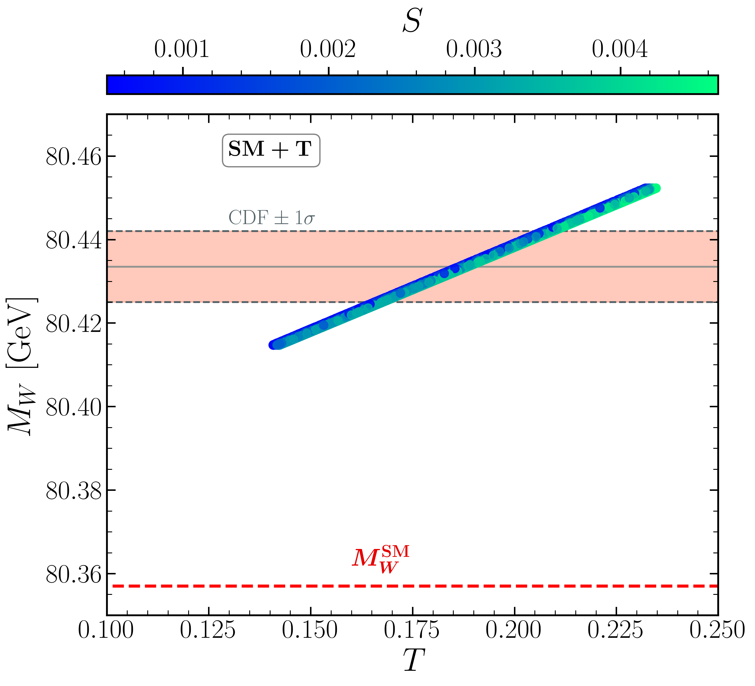
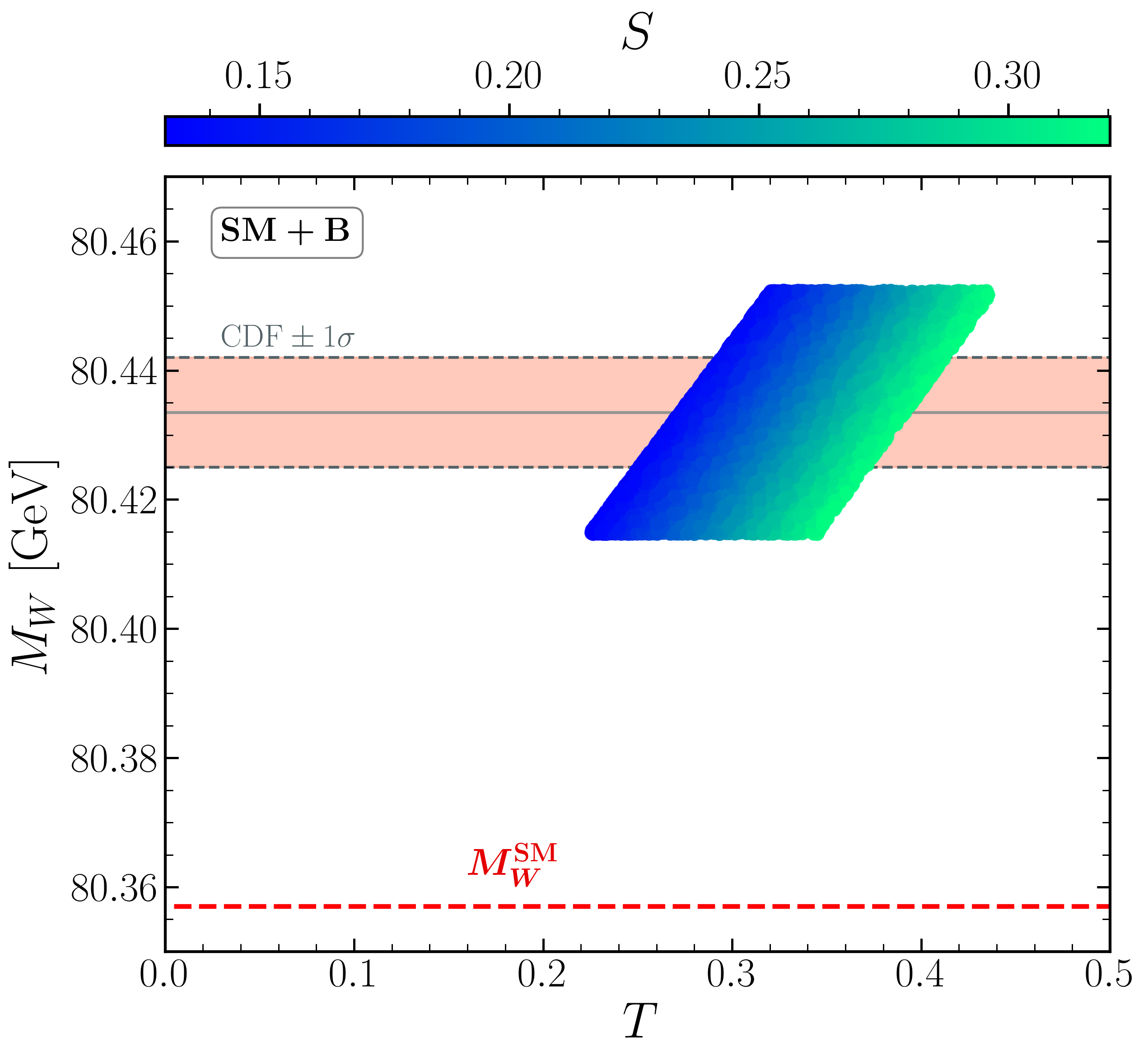
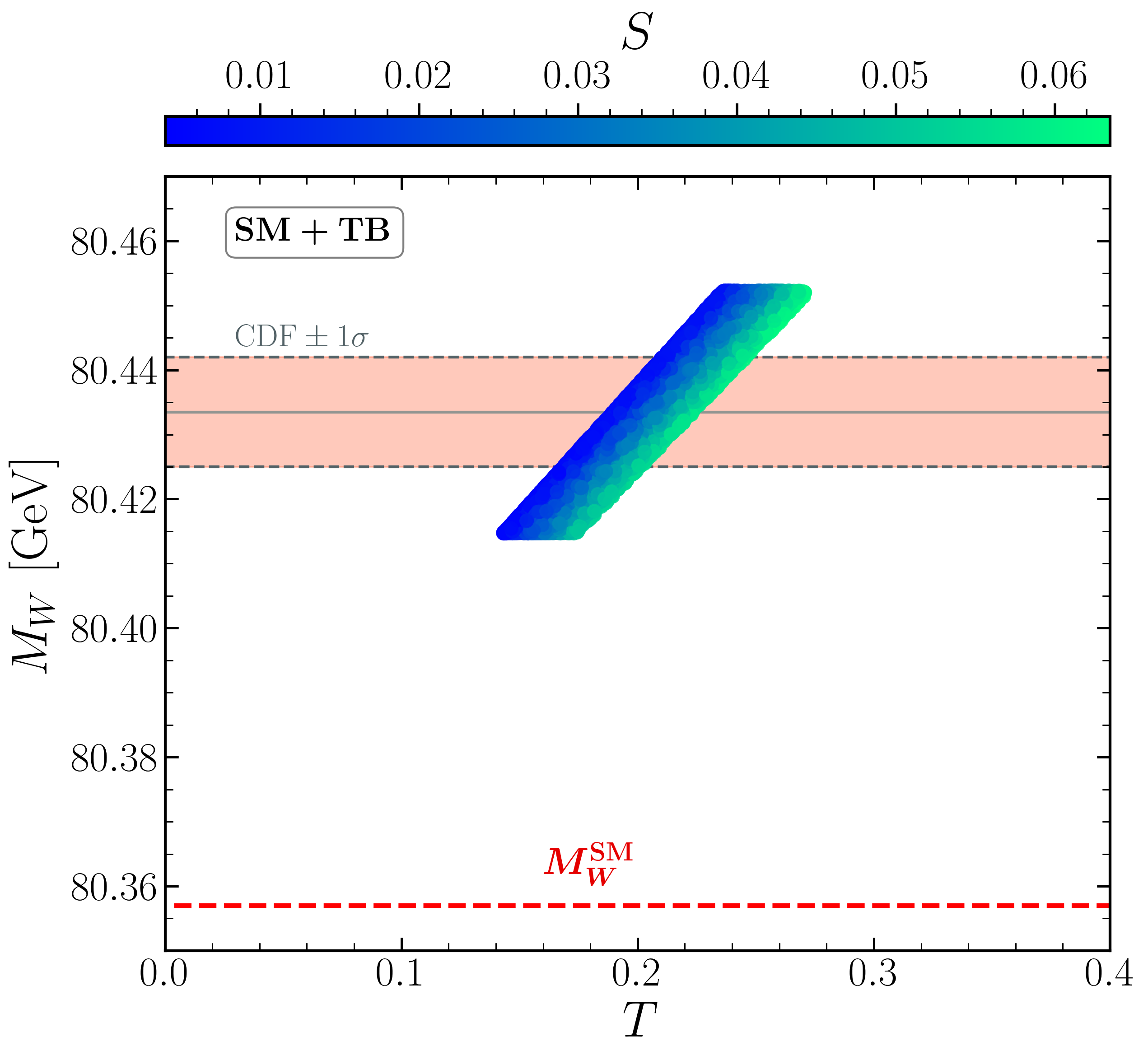
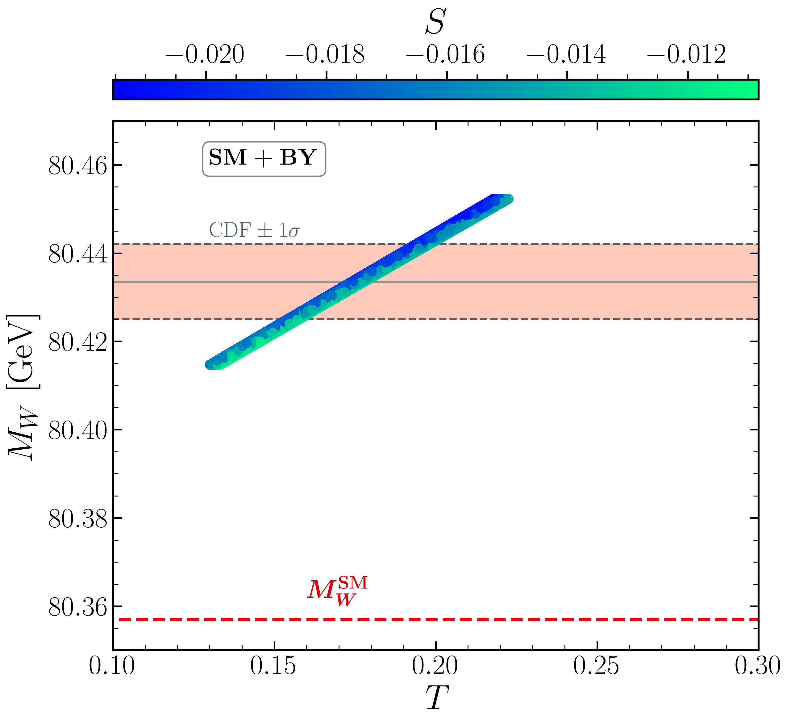
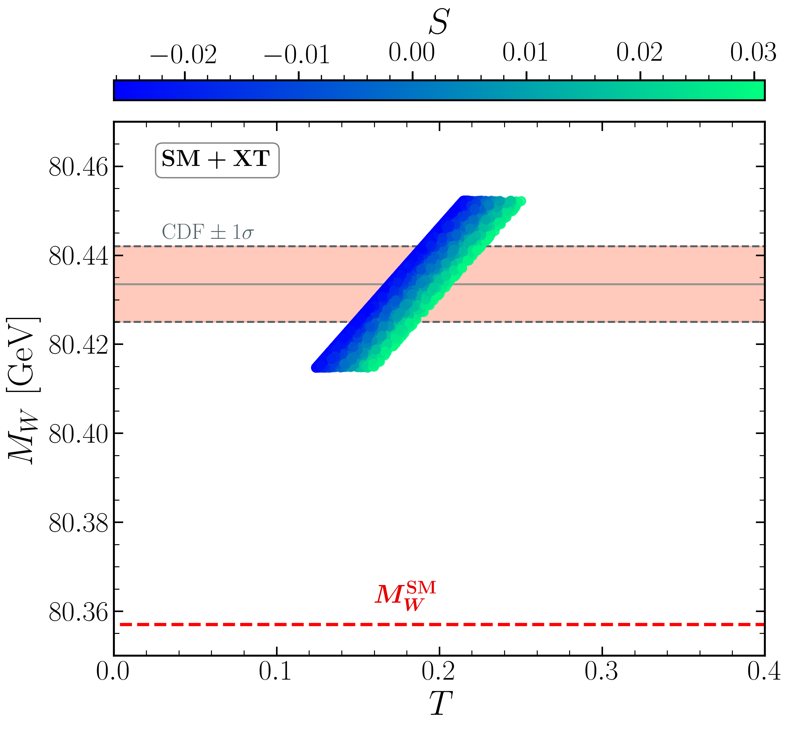
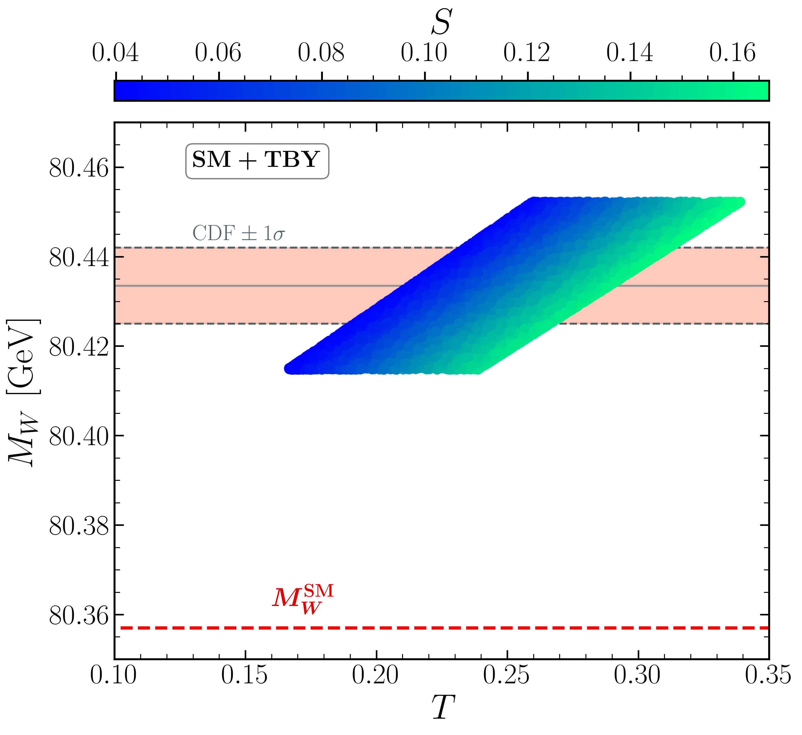
Figure 11: Scan result of the SM + (VLQs) in the $(T,M_{W})$. The light red band indicates the $M_{W}$ value with the associated 1$\sigma$ uncertainty measured recently by the CDF collaboration, while the light green band shows the result of $\sin^{2}\theta_{\mathrm{eff}}$ and its associated 1$\sigma$ uncertainty measured by the SLD collaboration.

In Fig. 11, we depict the $W$ mass calculated using Eq.28 as a function of the T parameter in the context of the SM + VLQs extensions. The oblique parameter $S$ is displayed on the color map. The orange band represents the new $M_{W}$ value measured by the CDF collaboration, along with its $1\sigma$ uncertainty. In all VLQs representations, the contribution of the T parameter required to explain the CDF’s newly measured W-boson mass is positive. While the $S$ parameter is only positively restricted in the SM + T,B,TB and TBY extension, it is negative in the SM + BY and XTB extension, and takes on both positive and negative values in the SM + XT extension.

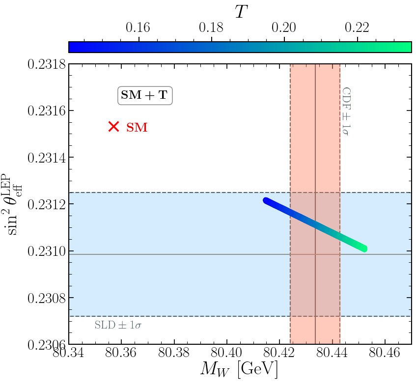
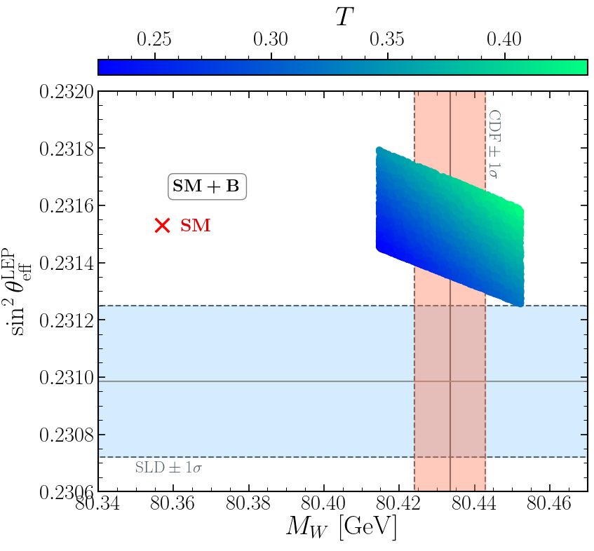
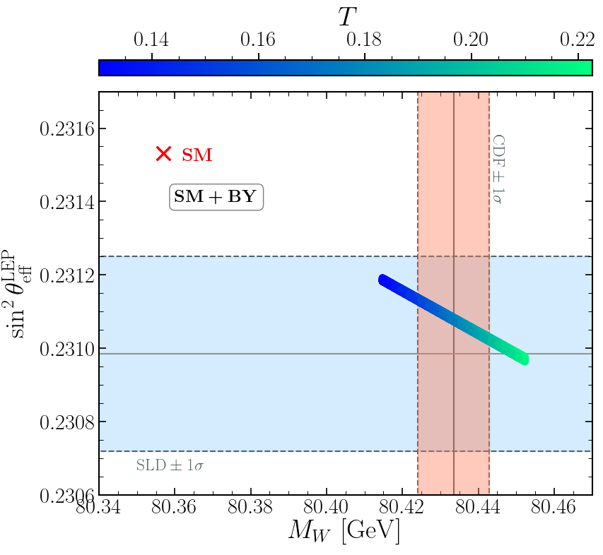
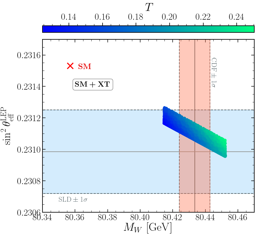
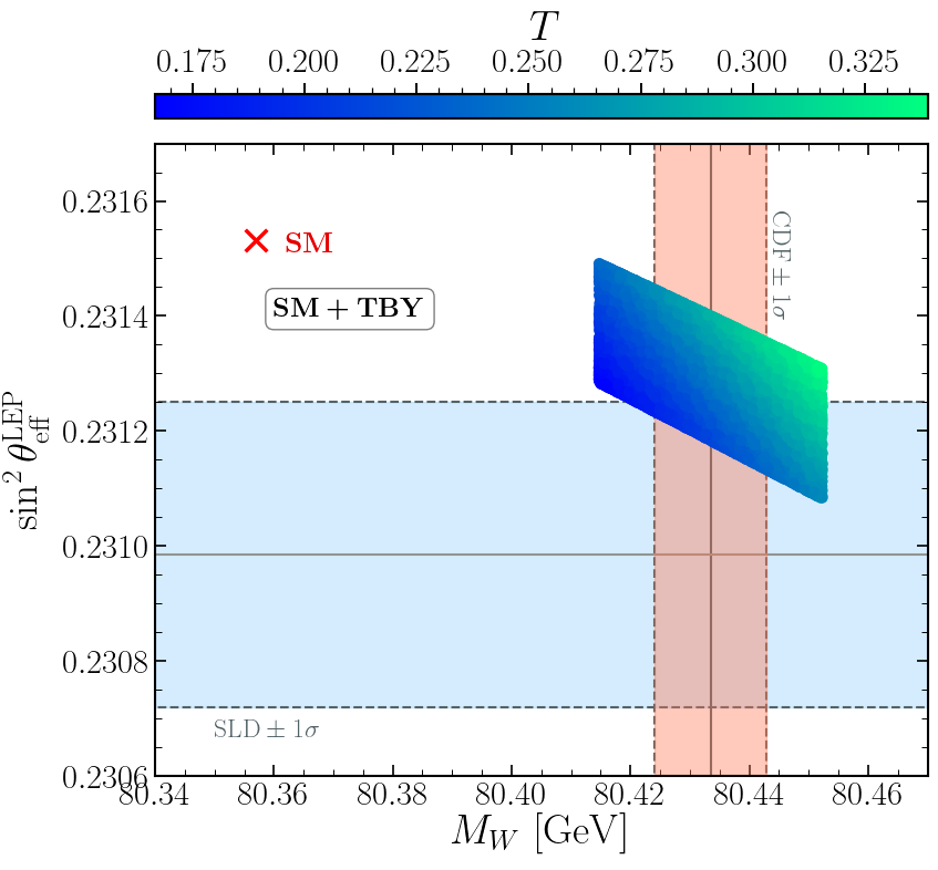
Figure 12: Scan result of the SM + (VLQs) in the $(M_{W},\sin^{2}\theta^{\mathrm{LEP}}_{\mathrm{eff}})$ plane. The light red band indicates the $M_{W}$ value with the associated 1$\sigma$ uncertainty measured recently by the CDF collaboration, while the light green band shows the result of $\sin^{2}\theta_{\mathrm{eff}}$ and its associated 1$\sigma$ uncertainty measured by the SLD collaboration.

In Fig. 12 we present the same points in the $(M_{W},\sin^{2}\theta^{\mathrm{LEP}}_{\mathrm{eff}})$ plane with the T parameter in the color bar. The light blue band represents the measurement of the SLD collaboration for $\sin^{2}\theta_{eff}$ within the $\pm 1\sigma$. It is interesting to see that the points satisfying the CDF-II data are in good agreement with the data points preferred by the SLD measurement of the $\sin^{2}\theta_{eff}$ within 1 $\sigma$ uncertainty in the case of SM+(T, BY and XTB) while the SM+(TB, XT and TBY) are only partially within the bands. Furthermore, it can be seen that within the SM+B singlet, there is a significant tension between the points preferred by the CDF-II data and the SLD measurement.

References

- [1] T. Aaltonen et al. [CDF], “High-precision measurement of the W boson mass with the CDF II detector” Science 376 (2022) no.6589, 170-176.
- [2] P. A. Zyla et al. [Particle Data Group],“Review of Particle Physics”, PTEP 2020 (2020) no.8, 083C01.
- [3] C. T. Lu, L. Wu, Y. Wu and B. Zhu, arXiv:1409.3199 [hep-ph],A. Broggio, E. J. Chun, M. Passera, K. M. Patel and S. K. Vempati, arXiv:2204.03796 [hep-ph],Y. Z. Fan, T. P. Tang, Y. L. S. Tsai and L. Wu, arXiv:2204.03693 [hep-ph], H. Song, W. Su and M. Zhang, arXiv:2204.05085 [hep-ph], H. Bahl, J. Braathen and G. Weiglein, arXiv:2204.05269 [hep-ph], K. S. Babu, S. Jana and V. P. K., arXiv:2204.05303 [hep-ph], T. Biekötter, S. Heinemeyer and G. Weiglein, arXiv:2204.05975 [hep-ph], X. F. Han, F. Wang, L. Wang, J. M. Yang and Y. Zhang, arXiv:2204.06505 [hep-ph], Y. Heo, D. W. Jung and J. S. Lee, arXiv:2204.05728 [hep-ph], Y. H. Ahn, S. K. Kang and R. Ramos, arXiv:2204.06485 [hep-ph],R. Benbrik, M. Boukidi and B. Manaut, arXiv:2204.11755 [hep-ph], H. Abouabid, A. Arhrib, R. Benbrik, M. Krab and M. Ouchemhou, arXiv:2204.12018 [hep-ph], G. Arcadi and A. Djouadi, arXiv:2204.08406 [hep-ph], K. Ghorbani and P. Ghorbani, arXiv:2204.09001 [hep-ph] , S. Lee, K. Cheung, J. Kim, C. T. Lu and J. Song, arXiv:2204.10338 [hep-ph], J. Kim, arXiv:2205.01437 [hep-ph], S. Hessenberger and W. Hollik, arXiv:2207.03845 [hep-ph], O. Atkinson, M. Black, C. Englert, A. Lenz and A. Rusov, arXiv:2207.02789 [hep-ph].
- [4] X. K. Du, Z. Li, F. Wang and Y. K. Zhang, arXiv:2204.05760 [hep-ph], A. Ghoshal, N. Okada, S. Okada, D. Raut, Q. Shafi and A. Thapa, arXiv:2204.07138 [hep-ph], S. Kanemura and K. Yagyu, arXiv:2204.07511 [hep-ph], A. Addazi, A. Marciano, A. P. Morais, R. Pasechnik and H. Yang, arXiv:2204.10315 [hep-ph], Y. Cheng, X. G. He, F. Huang, J. Sun and Z. P. Xing, arXiv:2208.06760 [hep-ph], H. Bahl, W. H. Chiu, C. Gao, L. T. Wang and Y. M. Zhong, arXiv:2207.04059 [hep-ph].
- [5] J. M. Yang and Y. Zhang, arXiv:2204.04202 [hep-ph] ,A. Strumia, arXiv:2204.04191 [hep-ph] ,K. Sakurai, F. Takahashi and W. Yin, arXiv:2204.04770 [hep-ph] ,X. Liu, S. Y. Guo, B. Zhu and Y. Li, arXiv:2204.04834 [hep-ph] ,L. Di Luzio, R. Gröber and P. Paradisi, arXiv:2204.05284 [hep-ph] ,P. Asadi, C. Cesarotti, K. Fraser, S. Homiller and A. Parikh, arXiv:2204.05283 [hep-ph] ,J. J. Heckman, arXiv:2204.05302 [hep-ph] ,E. Bagnaschi, J. Ellis, M. Madigan, K. Mimasu, V. Sanz and T. You, arXiv:2204.05260 [hep-ph] ,A. Paul and M. Valli, arXiv:2204.05267 [hep-ph] ,R. Balkin, E. Madge, T. Menzo, G. Perez, Y. Soreq and J. Zupan, arXiv:2204.05992 [hep-ph] ,M. Endo and S. Mishima, arXiv:2204.05965 [hep-ph] ,M. D. Zheng, F. Z. Chen and H. H. Zhang, arXiv:2204.06541 [hep-ph] ,L. M. Carpenter, T. Murphy and M. J. Smylie, arXiv:2204.08546 [hep-ph] ,O. Popov and R. Srivastava, arXiv:2204.08568 [hep-ph] ,T. A. Chowdhury, J. Heeck, S. Saad and A. Thapa, arXiv:2204.08390 [hep-ph] ,V. Cirigliano, W. Dekens, J. de Vries, E. Mereghetti and T. Tong, arXiv:2204.08440 [hep-ph] ,A. Bhaskar, A. A. Madathil, T. Mandal and S. Mitra, arXiv:2204.09031 [hep-ph] ,S. Baek, arXiv:2204.09585 [hep-ph]. ,J. Cao, L. Meng, L. Shang, S. Wang and B. Yang, arXiv:2204.09477 [hep-ph] ,J. Kawamura, S. Okawa and Y. Omura, arXiv:2204.07022 [hep-ph] ,K. I. Nagao, T. Nomura and H. Okada, arXiv:2204.07411 [hep-ph] ,K. Y. Zhang and W. Z. Feng, arXiv:2204.08067 [hep-ph] ,D. Borah, S. Mahapatra and N. Sahu, arXiv:2204.09671 [hep-ph] , A. Batra, S. K. A, S. Mandal and R. Srivastava, arXiv:2204.09376 [hep-ph], Q. Zhou and X. F. Han, arXiv:2204.13027 [hep-ph], J. W. Wang, X. J. Bi, P. F. Yin and Z. H. Yu, arXiv:2205.00783 [hep-ph], B. Barman, A. Das and S. Sengupta, arXiv:2205.01699 [hep-ph], R. Dcruz and A. Thapa, arXiv:2205.02217 [hep-ph], T. A. Chowdhury and S. Saad, arXiv:2205.03917 [hep-ph], J. Gao, D. Liu and K. Xie, arXiv:2205.03942 [hep-ph], G. Lazarides, R. Maji, R. Roshan and Q. Shafi, arXiv:2205.04824 [hep-ph], T. Li, J. Pei, X. Yin and B. Zhu, arXiv:2205.08215 [hep-ph], J. Kawamura and S. Raby, arXiv:2205.10480 [hep-ph], D. Van Loi and P. Van Dong, arXiv:2206.10100 [hep-ph], H. Song, X. Wan and J. H. Yu, arXiv:2211.01543 [hep-ph], A. L. Cherchiglia and O. L. G. Peres, arXiv:2209.12063 [hep-ph], V. Barger, C. Hauptmann, P. Huang and W. Y. Keung, arXiv:2208.06422 [hep-ph], W. Abdallah, R. Gandhi and S. Roy, arXiv:2208.02264 [hep-ph],K. I. Nagao, T. Nomura and H. Okada, arXiv:2206.15256 [hep-ph], B. A. Ouazghour, R. Benbrik, E. Ghourmin, M. Ouchemhou and L. Rahili, arXiv:2302.01641 [hep-ph], J. Wu, D. Huang and C. Q. Geng, arXiv:2212.14553 [hep-ph], N. Chakrabarty, I. Chakraborty, D. K. Ghosh and G. Saha, arXiv:2212.14458[hep-ph], S. Chai, J. Gu and L. T. Wang, arXiv:2212.09253 [hep-ph], D. W. Jung, Y. Heo and J. S. Lee, arXiv:2212.07620 [hep-ph].
- [6] J. A. Aguilar-Saavedra, R. Benbrik, S. Heinemeyer and M. Pérez-Victoria, Handbook of vectorlike quarks: Mixing and single production, Phys.Rev. D88, no. 9 (2013) 094010, arXiv:1306.0572[hep-ph].
- [7] A. Arhrib, R. Benbrik, S. J. D. King, B. Manaut, S. Moretti and C. S. Un, Phenomenology of 2HDM with vectorlike quarks, Phys.Rev. D97, no. 9 (2018) 095015, arXiv:1607.08517 [hep-ph].
- [8] G. Passarino and M. J. G. Veltman, ‘‘One Loop Corrections for e+ e- Annihilation Into mu+ mu- in the Weinberg Model’’, Nucl. Phys. B160 (1979), 151-20.
- [9] C. Anastasiou, C. Duhr, F. Dulat, E. Furlan, T. Gehrmann, F. Herzog, A. Lazopoulos and B. Mistlberger, ‘‘High precision determination of the gluon fusion Higgs boson cross-section at the LHC’’, JHEP 05 (2016), 058, arXiv:1602.00695 [hep-ph].
- [10] C. Anastasiou, S. Buehler, E. Furlan, F. Herzog and A. Lazopoulos, ‘‘Higgs production cross-section in a Standard Model with four generations at the LHC’’, Phys. Lett. B702 (2011), 224-227, arXiv:1103.3645 [hep-ph].
- [11] R. Benbrik, C. H. Chen and T. Nomura, Higgs singlet boson as a di-photon resonance in a vectorlike quark model, Phys.Rev. D93, no. 5 (2016) 055034, arXiv:1512.06028[hep-ph].
- [12] A. Angelescu, A. Djouadi and G. Moreau, Scenarii for interpretations of the LHC di-photon excess: two Higgs doublets and VLQs and leptons, Phys.Lett. B756 (2016) 126, arXiv:1512.04921[hep-ph].
- [13] J. A. Aguilar-Saavedra, Identifying top partners at LHC, JHEP 11 (2009) 030, [arXiv:0907.3155].
- [14] A. De Simone, O. Matsedonskyi, R. Rattazzi and A. Wulzer, A First Top Partner Hunter’s Guide, JHEP 04 (2013) 004, arXiv:1211.5663[hep-ph].
- [15] S. Kanemura, M. Kikuchi and K. Yagyu, Fingerprinting the extended Higgs sector using one-loop corrected Higgs boson couplings and future precision measurements, Nucl.Phys. B896 (2015) 80, arXiv:1502.07716[hep-ph].
- [16] L. Lavoura and J. P. Silva, The Oblique corrections from vector - like singlet and doublet quarks, Phys.Rev. D47, 2046 (1993).
- [17] C. Y. Chen, S. Dawson and E. Furlan, Vectorlike fermions and Higgs effective field theory revisited, Phys.Rev. D96 (2017) no.1, 015006, arXiv:1703.06134[hep-ph].
- [18] S. P. He, ‘‘A leptoquark and vector-like quark extended model for the simultaneous explanation of the boson mass and muon anomalies’’ , arXiv:2205.02088 [hep-ph].
- [19] J. Cao, L. Meng, L. Shang, S. Wang and B. Yang, ‘‘Interpreting the W-mass anomaly in vectorlike quark models’’, Phys.Rev. D106 (2022) no.5, 055042, arXiv:2204.09477 [hep-ph].
- [20] A. Carvalho, S. Moretti, D. O’Brien, L. Panizzi and H. Prager, Single production of vectorlike quarks with large width at the Large Hadron Collider, Phys.Rev. D98 (2018) no.1, 015029, arXiv:1805.06402[hep-ph].
- [21] S. Moretti, D. O’Brien, L. Panizzi and H. Prager, Production of extra quarks at the Large Hadron Collider beyond the Narrow Width Approximation, Phys.Rev. D96 (2017) no.7, 075035, arXiv:1603.09237[hep-ph].
- [22] H. Prager, S. Moretti, D. O’Brien and L. Panizzi, Large width effects in processes of production of extra quarks decaying to Dark Matter at the LHC, PoS DIS 2017 (2018) 300, arXiv:1706.04007[hep-ph].
- [23] H. Prager, S. Moretti, D. O’Brien and L. Panizzi, Extra Quarks Decaying to Dark Matter Beyond the Narrow Width Approximation, arXiv:1706.04001[hep-ph].
- [24] S. Moretti, D. O’Brien, L. Panizzi and H. Prager, Production of extra quarks decaying to Dark Matter beyond the Narrow Width Approximation at the LHC, Phys.Rev. D96 (2017) no.3, 035033, arXiv:1705.07675[hep-ph].
- [25] A. Deandrea and A.M. Iyer, Vector-like quarks and heavy coloured bosons at the LHC, Phys.Rev.D97, no. 5 (2018) 055002, [arXiv:1710.01515[hep-ph]].
- [26] J. A. Aguilar-Saavedra, D. E. López-Fogliani and C. Muoz, Novel signatures for VLQs, JHEP 06 (2017) 095, [arXiv:1705.02526[hep-ph]].
- [27] C. Anastasiou, E. Furlan and J. Santiago, ‘‘Realistic Composite Higgs Models’’, Phys.Rev. D79 (2009), 075003, arXiv:0901.2117 [hep-ph].
- [28] R. Contino, ‘‘The Higgs as a Composite Nambu-Goldstone Boson’’, arXiv:1005.4269 [hep-ph].
- [29] K. Agashe and R. Contino, ‘‘The Minimal composite Higgs model and electroweak precision tests’’, Nucl. Phys. B742 (2006), 59-85, arXiv:hep-ph/0510164 [hep-ph].
- [30] G. Panico and A. Wulzer, ‘‘The Composite Nambu-Goldstone Higgs’’, Lect. Notes Phys. 913 (2016), pp.1-316, arXiv:1506.01961 [hep-ph].
- [31] M. Gillioz, R. Grober, C. Grojean, M. Muhlleitner and E. Salvioni, ‘‘Higgs Low-Energy Theorem (and its corrections) in Composite Models’’, JHEP 10 (2012), 004, arXiv:1206.7120 [hep-ph].
- [32] R. Benbrik, M. Boukidi and S. Moretti, ‘‘Probing Light Charged Higgs Bosons in the 2-Higgs Doublet Model Type-II with Vector-Like Quarks’’, arXiv:2211.07259 [hep-ph].
- [33] N. Arkani-Hamed, A. G. Cohen, E. Katz and A. E. Nelson, ‘‘The Littlest Higgs’’, JHEP 07 (2002), 034, arXiv:hep-ph/0206021 [hep-ph].
- [34] J. Hubisz and P. Meade, ‘‘Phenomenology of the littlest Higgs with T-parity’’, Phys.Rev. D71 (2005), 035016t, arXiv:hep-ph/0411264 [hep-ph].
- [35] T. Han, H. E. Logan, B. McElrath and L. T. Wang, ‘‘Phenomenology of the little Higgs model’’, Phys.Rev. D67 (2003), 095004, arXiv:hep-ph/0301040 [hep-ph].
- [36] CMS, ‘‘Search for pair production of vector-like quarks in leptonic final states in proton-proton collisions at = 13 TeV’’, arXiv:2209.07327 [hep-ex].
- [37] ATLAS, T. Vale, ‘‘Search for pair-production of vector-like quarks in final states with at least one boson decaying into a pair of electrons or muons in collision data collected with the ATLAS detector at = 13 TeV’’, arXiv:1812.02112 [hep-ex].
- [38] G. C. Branco, P. M. Ferreira, L. Lavoura, M. N. Rebelo, M. Sher and J. P. Silva, ‘‘Theory and phenomenology of two-Higgs-doublet models’’, Phys. Rept. 516 (2012), 1-102xt, arXiv:1106.0034 [hep-ph].
- [39] S. L. Glashow and S. Weinberg, ‘‘Natural Conservation Laws for Neutral Currents’’, Phys. Rev D15 (1977), 1958.
- [40] M. E. Peskin and T. Takeuchi,‘‘A New constraint on a strongly interacting Higgs sector’’ Phys. Rev. Lett. 65 (1990), 964-967.
- [41] M. E. Peskin and T. Takeuchi,‘‘Estimation of oblique electroweak corrections’’, Phys. Rev. D46 (1992), 381-409.
- [42] W. Grimus, L. Lavoura, O. M. Ogreid and P. Osland,‘‘The Oblique parameters in multi-Higgs-doublet models’’, Nucl. Phys. B801 (2008),arXiv:0802.4353 [hep-ph]. [43]28
- [43] T. Biekötter, S. Heinemeyer and G. Weiglein, ‘‘Excesses in the low-mass Higgs-boson search and the W-boson mass measurement’’, arXiv:2204.05975 [hep-ph].
- [44] T. Hahn, ‘‘Loop calculations with FeynArts, FormCalc, and LoopTools’’, Acta Phys. Polon. B30 (1999), 3469-3475, arXiv:hep-ph/9910227 [hep-ph].
- [45] T. Hahn, ‘‘Feynman Diagram Calculations with FeynArts, FormCalc, and LoopTools’’, PoS ACAT2010 (2010), 078, arXiv:1006.2231 [hep-ph].
- [46] D. Eriksson, J. Rathsman and O. Stal, ‘‘2HDMC: Two-Higgs-Doublet Model Calculator Physics and Manual,’’ Comput. Phys. Commun. 181 (2010) 189-205, arXiv:0902.0851 [hep-ph].
- [47] T. Hahn, Generating Feynman diagrams and amplitudes with FeynArts 3, Comput. Phys. Commun. 140 (2001) 418, [arXiv:0012260[hep-ph]].
- [48] T. Hahn and C. Schappacher, The Implementation of the minimal supersymmetric standard model in FeynArts and FormCalc, Comput. Phys. Commun. 143 (2002) 54, [arXiv:hep-ph/0105349 [hep-ph]].
- [49] S. Kanemura, T. Kubota and E. Takasugi, ‘‘Lee-Quigg-Thacker bounds for Higgs boson masses in a two doublet model’’, Phys. Lett. B313 (1993) 155-160, arXiv:hep-ph/9303263 [hep-ph].
- [50] A. G. Akeroyd, A. Arhrib and E. M. Naimi, ‘‘Note on tree level unitarity in the general two Higgs doublet model’’, Phys. Lett. B490 (2000) 119-124, arXiv:hep-ph/0006035 [hep-ph].
- [51] A. Arhrib, ‘‘Unitarity constraints on scalar parameters of the standard and two Higgs doublets model’’, arXiv:hep-ph/0012353 [hep-ph].
- [52] A. Barroso, P. M. Ferreira, I. P. Ivanov and R. Santos, ‘‘Metastability bounds on the two Higgs doublet model’’, JHEP 06 (2013), 045, arXiv:1303.5098 [hep-ph].
- [53] N. G. Deshpande and E. Ma, ‘‘Pattern of Symmetry Breaking with Two Higgs Doublets’’, Phys. Rev. D18 (1978) 2574.
- [54] P. Bechtle, O. Brein, S. Heinemeyer, G. Weiglein and K. E. Williams, HiggsBounds: Confronting Arbitrary Higgs Sectors with Exclusion Bounds from LEP and the Tevatron, Comput. Phys. Commun. 181 (2010), arXiv:0811.4169 [hep-ph].
- [55] P. Bechtle, O. Brein, S. Heinemeyer, G. Weiglein and K. E. Williams, HiggsBounds 2.0.0: Confronting Neutral and Charged Higgs Sector Predictions with Exclusion Bounds from LEP and the Tevatron, Comput. Phys. Commun. 182 (2011), 2605-2631, arXiv:1102.1898 [hep-ph].
- [56] P. Bechtle, O. Brein, S. Heinemeyer, O. Stål, T. Stefaniak, G. Weiglein and K. E. Williams, HiggsBounds-4: Improved Tests of Extended Higgs Sectors against Exclusion Bounds from LEP, the Tevatron and the LHC, Eur. Phys. J. C74 (2014) no.3, 2693, arXiv:1311.0055 [hep-ph].
- [57] P. Bechtle, S. Heinemeyer, O. Stål, T. Stefaniak and G. Weiglein, Probing the Standard Model with Higgs signal rates from the Tevatron, the LHC and a future ILC, JHEP 11 (2014), 039, [arXiv:1403.1582 [hep-ph]].
- [58] P. Bechtle, S. Heinemeyer, O. Stal, T. Stefaniak and G. Weiglein, Applying Exclusion Likelihoods from LHC Searches to Extended Higgs Sectors, Eur. Phys. J. C75 (2015) no.9, 421, [1507.06706].
- [59] P. Bechtle, D. Dercks, S. Heinemeyer, T. Klingl, T. Stefaniak, G. Weiglein and J. Wittbrodt, HiggsBounds-5: Testing Higgs Sectors in the LHC 13 TeV Era, Eur. Phys. J. C80 (2020) 1211, [arXiv:2006.06007 [hep-ph]].
- [60] P. Bechtle, S. Heinemeyer, O. Stål, T. Stefaniak and G. Weiglein, =HiggsSignals: Confronting arbitrary Higgs sectors with measurements at the Tevatron and the LHC, Eur. Phys. J. C74 (2014) no.2, 2711, [arXiv:1305.1933 [hep-ph]].
- [61] P. Bechtle, S. Heinemeyer, T. Klingl, T. Stefaniak, G. Weiglein and J. Wittbrodt, HiggsSignals-2: Probing new physics with precision Higgs measurements in the LHC 13 TeV era, Eur. Phys. J. C81 (2021) 145, [arXiv:2012.09197 [hep-ph]].
- [62] F. Mahmoudi, ‘‘SuperIso v2.3: A Program for calculating flavor physics observables in Supersymmetry’’, Comput. Phys. Commun. 180 (2009) 1579-1613, arXiv:0808.3144 [hep-ph].
- [63] Y. Amhis et al. [HFLAV], ‘‘Averages of -hadron, -hadron, and -lepton properties as of summer 2016’’, Eur. Phys. J. C77 (2017) no.12, 895 , arXiv:1612.07233 [hep-ex].
- [64] R. Aaij et al. [LHCb], ‘‘Measurement of the branching fraction and effective lifetime and search for decays’’, Phys. Rev. Lett. 118 (2017) no.19, 191801, arXiv:1703.05747 [hep-ex].
- [65] W. Grimus, L. Lavoura, O. M. Ogreid and P. Osland, ‘‘A Precision constraint on multi-Higgs-doublet models’’, J. Phys. G35 (2008), 075001, arXiv:0711.4022 [hep-ph].
- [66] W. Grimus, L. Lavoura, O. M. Ogreid and P. Osland, ‘‘The Oblique parameters in multi-Higgs-doublet models’’, Nucl. Phys. B801 (2008) 81-96, arXiv:0802.4353 [hep-ph].
- [67] J. Haller, A. Hoecker, R. Kogler, K. Mönig, T. Peiffer and J. Stelzer, ‘‘Update of the global electroweak fit and constraints on two-Higgs-doublet models’’, Eur. Phys. J. C78 (2018) no.8, 675, arXiv:1803.01853 [hep-ph].
- [68] Particle Data Group Collaboration, P. Zyla et al., ‘‘Review of Particle Physics’’, Progress of Theoretical and Experimental Physics 2020 no. 8 (2020) 083C01.
- [69] T. Hahn, S. Paßehr and C. Schappacher, ‘FormCalc 9 and Extensions’’, PoS LL2016 (2016), 068, arXiv:1604.04611 [hep-ph].
- [70] J. Kublbeck, M. Bohm and A. Denner, Feyn Arts: Computer Algebraic Generation of Feynman Graphs and Amplitudes, Comput. Phys. Commun. 60 (1990), 165-180.
- [71] T. Hahn and M. Perez-Victoria, Automatized one loop calculations in four-dimensions and D-dimensions, Comput. Phys. Commun. 118 (1999) 153, [arXiv:hep-ph/9807565 [hep-ph]].
- [72] S. Schael et al. [ALEPH, DELPHI, L3, OPAL, SLD, LEP Electroweak Working Group, SLD Electroweak Group and SLD Heavy Flavour Group], ‘‘Precision electroweak measurements on the resonance’’, Phys. Rept. 427 (2006), 257-454, arXiv:hep-ex/0509008 [hep-ex].