Kinetic Axion Dark Matter in String Corrected $f(R)$ Gravity

Abstract

Under the main assumption that the axion scalar field mainly composes the dark matter in the Universe, in this paper we shall extend the formalism of kinetic axion $R^{2}$ gravity to include Gauss-Bonnet terms non-minimally coupled to the axion field. As we demonstrate, this non-trivial Gauss-Bonnet term has dramatic effects on the inflationary phenomenology and on the kinetic axion scenario. Specifically, in the context of our formalism, the kinetic axion ceases to be kinetically dominated at the end of the inflationary era, since the condition $\dot{\phi}\simeq 0$ naturally emerges in the theory. Thus, unlike the case of kinetic axion $R^{2}$ gravity, the Gauss-Bonnet corrected kinetic axion $R^{2}$ gravity leads to an inflationary era which is not further extended and the reheating era commences right after the inflationary era, driven by the $R^{2}$ fluctuations.

I Introduction

Dark matter is still mysterious to date, since no evidence of this elusive dark component of our Universe has been found to date. The particle nature of dark matter is very well motivated, since evidence of dark matter halos around spiral galaxies, and cosmic events like the bullet cluster point to a particle nature of dark matter. In the past, many candidate particle were proposed to describe particle dark matter [1, 2, 3, 4, 5, 6], to date no evidence for a dark matter particle has ever been found. This is probably because earlier studies and experiments focused to Weakly Interacting Massive Particles (WIMPs), with masses ranging from 100 MeV to hundreds GeV. Thus currently the interest of cosmologists is turned to light dark matter particle candidates. The prominent candidate for a large amount of phenomenological reasons is the axion, see Refs. [7, 8, 9, 10, 11, 12, 13, 14, 15, 16, 17, 18, 19, 20, 21, 22, 23, 24, 25, 26, 27, 28, 29, 30, 31, 32, 33, 34, 35, 36, 37, 38, 39, 40, 41, 42, 43, 44, 45, 46, 47, 48, 49, 50, 51, 52, 53, 54, 55, 56, 57, 58, 59, 60, 61, 62, 63, 64, 65, 66, 67, 68, 69, 70, 71, 72, 73, 74, 75, 76, 77, 78, 79, 80, 81, 82, 83, 84], for an important stream of articles and reviews, and also [85, 11] for some recent updated reviews. Some interesting simulations can also be found in [86] which predict a mass for the axion of the $\mu$eV order and in [87] an experimental proposal was introduced. Furthermore, an interesting explanation of the recent Gamma ray bursts observations [88, 89] can be provided by axion-like particles with masses of the order $m_{a}\sim\mathcal{O}(10^{-10})\,$eV. Among axion models, the most important and phenomenologically appealing are the ones that have their primordial Peccei-Quinn $U(1)$ symmetry broken during inflation, unlike in the QCD axion. These belong to the class of misalignment axion models, with two characteristic candidates, the canonical misalignment model [10] and the kinetic axion model [17, 18, 19]. In both models, the axion is misaligned from the minimum of its potential, however in the canonical misalignment has no initial kinetic energy, while in the kinetic misalignment it possesses a large kinetic energy. Hence, this excess in the kinetic energy delays the axion oscillations which start when the axion reaches its minimum and when the axion mass $m_{a}$ becomes of the same order as the Hubble rate, that is $m_{a}\sim H$.

In a previous work [71] we studied the effects of the kinetic axion on the $R^{2}$ inflation theory. As we showed, although the axion effects are insignificant during the inflationary era, the kinetic axion dominates the early post-inflationary era, dominating over the $\langle R^{2}\rangle$ fluctuations, which effectively destabilize the quasi-de Sitter vacuum $R^{2}$ attractor. Thus post-inflationary the Universe experiences a short stiff era controlled by the axion, before the latter settles in the minimum of its potential, starting its oscillations and having an energy density redshifting as dark matter. In this article, we aim to study the effects of string corrections in the kinetic axion $R^{2}$ Lagrangian, in the form of Einstein-Gauss-Bonnet corrections. The motivation to have a scalar field and considering modified gravity corrections of the form of higher curvature invariants comes from the fact that the standard four dimensional vacuum configuration scalar field Lagrangian,

$$\mathcal{S}_{\varphi}=\int d^{4}x\sqrt{-g}\left(\frac{1}{2}Z(\varphi)g^{\mu\nu}\partial_{\mu}\varphi\partial_{\nu}\varphi+\mathcal{V}(\varphi)+h(\varphi)\mathcal{R}\right)\,,$$ (1)

in which the scalar field must be either conformally or minimally coupled, receives the following one loop quantum corrections [90, 91]

$$\mathcal{S}_{eff}=\int d^{4}x\sqrt{-g}\Big{(}\Lambda_{1}+\Lambda_{2}\mathcal{R}+\Lambda_{3}\mathcal{R}^{2}+\Lambda_{4}\mathcal{R}_{\mu\nu}\mathcal{R}^{\mu\nu}+\Lambda_{5}\mathcal{R}_{\mu\nu\alpha\beta}\mathcal{R}^{\mu\nu\alpha\beta}+\Lambda_{6}\square\mathcal{R}$$ (2)

$$+\Lambda_{7}\mathcal{R}\square\mathcal{R}+\Lambda_{8}\mathcal{R}_{\mu\nu}\square\mathcal{R}^{\mu\nu}+\Lambda_{9}\mathcal{R}^{3}+\mathcal{O}(\partial^{8})+...\Big{)}\,,$$

with the parameters $\Lambda_{i}$, $i=1,2,...,6$ being some dimensionful constants, see also the interesting Ref. [92] for extra Chern-Simons corrections on the quantum action. The above corrections contain fourth order derivatives and the action is compatible with diffeomorphism invariance. Apparently, in our case the axion scalar field during inflation is described by $Z(\varphi)=-1$ and $h(\varphi)=1$ in the action (1). Having modified gravity in its various forms [93, 94, 95, 96, 97] driving inflation and possibly the dark energy era, a viable framework is offered in which inflation and the dark energy era may be described by the same theory [98, 99, 100, 101, 102, 103, 104, 68, 105]. Before we proceed, it should be stated that throughout this paper, a homogeneous and isotropic background shall be considered with the line element being,

$$\centering ds^{2}=-dt^{2}+a^{2}(t)\delta_{ij}dx^{i}dx^{j}\,,\@add@centering$$ (3)

where $a(t)$ stands for the scale factor. In turn, the axion field is assumed to be homogeneous as well therefore hereafter, $\phi=\phi(t)$. This simplifies a lot the subsequent calculations and it is a well motivated assumption.

II kinetic axion $f(R)$ gravity with string corrective terms

In the literature, the axion dynamics have been investigated for a plethora of models, since it is a prominent candidate for non-thermal dark matter. In this paper, based on this assumption, we shall investigate the inflationary phenomenology of the kinetic axion model in the presence of higher order curvature invariants. In particular, we shall make use of an $f(R)$ model which is known for producing viable inflationary phenomenology, while furthermore a non-minimal coupling between the axion and the Gauss-Bonnet density shall be considered, in order to explicitly have a coupling between the scalar field and curvature. Hence, in order to study the primordial era of our Universe, the following gravitational action is proposed,

$$\centering\mathcal{S}=\int d^{4}x\sqrt{-g}\bigg{(}\frac{f(R)}{2\kappa^{2}}-\frac{1}{2}g^{\mu\nu}\nabla_{\mu}\phi\nabla_{\nu}\phi-V(\phi)-\xi(\phi)\mathcal{G}\bigg{)}\,,\@add@centering$$ (4)

where $R$ is the Ricci scalar, $\kappa=\frac{1}{M_{P}}$ with $M_{P}=1/\sqrt{8\pi G}$ being the reduced Planck mass, $\frac{1}{2}g^{\mu\nu}\nabla_{\mu}\phi\nabla_{\nu}\phi$ and $V(\phi)$ stand for the kinetic term and the canonical scalar field potential, while $\xi(\phi)$ is the arbitrary for the time being scalar coupling function of the axion to the Gauss-Bonnet invariant, which shall be specified subsequently and $\mathcal{G}=R^{\mu\nu\rho\sigma}R_{\mu\nu\rho\sigma}-4R^{\mu\nu}R_{\mu\nu}+R^{2}$ is the Gauss-Bonnet invariant with $R_{\mu\nu}$ and $R_{\mu\nu\rho\sigma}$ being the Ricci and Riemann tensor respectively. In this model, there are two tensor degrees of freedom, and an additional scalar mode coming from the $f(R)$ gravity. Here, it should be stated that in order to have a direct impact of the Gauss-Bonnet density in the overall phenomenology, a non-trivial coupling is required due to the fact that the model is studied in $D=4$, hence the reason why the arbitrary function $\xi(\phi)$ is introduced. This inclusion has a major impact on the overall phenomenology as we shall showcase explicitly. It should also be stated that recently, an additional approach has been considered where by working initially in $D$ dimensions and introducing the Gauss-Bonnet density in the gravitational action without a non-trivial coupling but with a constant factor scaling as $\frac{\alpha}{D-4}$, it is possible to keep such contribution in the limit $D\to 4$ as it was shown in Ref. [106], however this approach, although worthy of being mentioned, shall not be considered here. This is because the non-minimal coupling between the scalar field and the Gauss-Bonnet density in this case affects the continuity equation of the scalar field compared to the case of [71], and thus a completely new territory is explored. Before we proceed with the equations of motion and the inflationary phenomenology, a quick statement on the Gauss-Bonnet term and its impact on tensor perturbations should be made.

By including the Gauss-Bonnet density in Eq. (4), the continuity equation of the scalar field, and in consequence the scalar perturbations, are not the only objects that are affected. This inclusion is known for being a subclass of Horndeski’s theory and thus the propagation velocity of tensor perturbations is also influenced by such term. According to Ref. [107], one can show that the deviation of the propagation speed of tensor perturbations from the speed of light is quantified by the following expression,

$$\centering c_{\mathcal{T}}^{2}=1-\frac{Q_{f}}{Q_{t}}\,,\@add@centering$$ (5)

where $Q_{f}=8(\ddot{\xi}-H\dot{\xi})$ and $Q_{t}=\frac{1}{\kappa^{2}}\frac{df}{dR}-8\dot{\xi}H$ are auxiliary parameters. Recently, the GW170817 event indicated explicitly that gravitational waves propagate throughout spacetime with the velocity of light, therefore theories which predict a different result have been excluded. In this case however, one can postulate that the arbitrary Gauss-Bonnet scalar coupling function is not so arbitrary but it needs to satisfy the differential equation,

$$\centering\ddot{\xi}=H\dot{\xi}\,,\@add@centering$$ (6)

which in turn implies that the auxiliary parameter $Q_{f}$ in Eq. (5) vanishes identically. As a result, the Gauss-Bonnet models that respect this constraint can actually be in agreement with the latest observations. At this point, one may argue that the constraint is not necessarily needed because the behavior of $\phi$, and in consequence $\xi(\phi)$ differs between early and late-time. It could be the case that while primordially the scalar field has a dynamical evolution that in consequence predicts $c_{\mathcal{T}}^{2}<1$, the scalar field freezes at late times, resulting in the conditions $\dot{\xi}=0=\ddot{\xi}$ and thus being in agreement with the GW170817 event in the late-time era only. But it hard to see how this statement could be realized in the standard cosmological evolution of the Universe post-inflationary. There is no fundamental reasoning emanating from particle physics that could allow the graviton to be massive initially and only at late times it becomes massless. Thus in the present article we shall avoid this argument and focus solely on the inflationary phenomenology of the constrained Gauss-Bonnet model. The Gauss-Bonnet model is a string inspired model and serves as a low-energy effective theory, so during and after inflation, the gravitons should be massless. Hence our massless graviton approach is well justified. Thus the constraint on the velocity of tensor perturbations shall be implemented in order to predict massless gravitons throughout the evolution of the Universe. Therefore, the constraint (6) will have a major impact on the continuity equation and in turn, it will influence the evolution of the scalar field. In Ref. [108], it was proved that the constraint decreases the overall degrees of freedom and one can treat the continuity equation of the scalar field as a differential equation from which a scalar function, either the potential or the Gauss-Bonnet scalar coupling function, are specified. Here, since we know the behaviour of the kinetic axion model, the usual approach shall be considered where the derivative of the scalar field is specified from the continuity equation once the Gauss-Bonnet scalar coupling function is designated. This is possible due to the fact that Eq. (6) can be rewritten by making use of the chain rule $\dot{\xi}=\xi^{\prime}\dot{\phi}$ as,

$$\centering\ddot{\phi}=H\dot{\phi}\bigg{[}1-\frac{\xi^{\prime\prime}}{H\xi^{\prime}}\dot{\phi}\bigg{]}\,,\@add@centering$$ (7)

where for simplicity, differentiation with respect to the scalar field is denoted with the “prime”. This equation is of paramount importance, since not only does it facilitate the derivation of $\dot{\phi}$ from the continuity equation, but it is also connected to one of the slow-roll indices that we are interested in, as we shall showcase in the following. Now at this stage, a few comments on the kinetic axion and canonical misalignment axion models should be made. We shall mainly focus on the kinetic axion model, but it is worth presenting both the kinetic and canonical misalignment axion models for completeness. Both the canonical misalignment and kinetic axion models belong to the class of misalignment axion models [10, 17], in which case the pre-inflationary Peccei-Quinn $U(1)$ symmetry is basically broken during the inflationary era and the axion field has an initial misalignment from the minimum of its potential. In this misalignment position, its vacuum expectation value is quite large $\phi_{i}\sim\theta f_{a}$, with $f_{a}$ being the axion decay constant, with $f_{a}>10^{9}\,$GeV, and $\theta$ is the misalignment angle, taking values in the range $0<\theta<1$. The general axion potential, after the breaking of the primordial Peccei-Quinn $U(1)$ symmetry has the form,

$$V_{a}(\phi)=m_{a}^{2}f_{a}^{2}\left(1-\cos\left(\frac{\phi}{f_{a}}\right)\right)\,.$$ (8)

When $\phi/f_{a}<1$, we can approximate the misalignment axion potential in the following way,

$$V_{a}(\phi)\simeq\frac{1}{2}m_{a}^{2}\phi^{2}\,.$$ (9)

Now regarding the initial kinetic energy of the axion, there are two mainstream models, the canonical misalignment axion [10] and the kinetic axion model [17]. In the former case, the axion rolls from its misalignment position towards the minimum of the potential with zero kinetic energy, and in the latter scenario the axion has a large kinetic energy. In the canonical misalignment model, when the axion reaches the potential minimum, and exactly when the Hubble rate satisfies $H\sim m_{a}$, the axion commences oscillations and its energy density $\rho_{a}$ redshifts as cold dark matter $\rho_{a}\sim a^{-3}$. In the kinetic axion case, the oscillations era starts at a much more later time compared to the canonical misalignment because the kinetic energy of the axion allows it to surpass the potential minimum and climbs up the potential, as it is shown in Fig. 1. In this case, the inflationary era lasts for more $e$-foldings [71, 70] and the reheating temperature must be smaller compared to the canonical misalignment one.

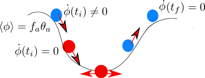
Figure 1: The canonical and kinetic misalignment models.

Since the constraint on the propagation velocity of gravitational waves and the mechanism for the kinetic axion have been briefly discussed, let us proceed with the inflationary phenomenology. According to the gravitational action (4) and the constraint (6), the equations of motion read,

$$\centering\frac{3FH^{2}}{\kappa^{2}}=\frac{1}{2}\dot{\phi}^{2}+V+24\dot{\xi}H^{3}+\frac{FR-f}{2\kappa^{2}}-\frac{3H\dot{F}}{\kappa^{2}}\,,\@add@centering$$ (10)

$$\centering-\frac{2F\dot{H}}{\kappa^{2}}=\dot{\phi}^{2}-16\dot{\xi}H\dot{H}+\frac{\ddot{F}-H\dot{F}}{\kappa^{2}}\,,\@add@centering$$ (11)

$$\centering\ddot{\phi}+3H\dot{\phi}+V^{\prime}+\xi^{\prime}\mathcal{G}=0\,,\@add@centering$$ (12)

where for simplicity we introduced the notation, $F=\frac{df}{dR}$. In order to simplify the analysis, we introduce two dimensionless auxiliary variables $x=\frac{\kappa^{2}\dot{\phi}^{2}}{6FH^{2}}$ and $y=-\frac{4\kappa^{2}\dot{\xi}H}{F}$ which participate in the first two equations. In order to proceed, and by following [71], the aforementioned parameters have a negligible contribution compared to the rest terms and, due to the fact that the axion mass is quite small and the potential and kinetic terms of the axion are inferior to the modified gravity terms. Thus, one finds that the background field equations can be approximated as,

$$\centering 3FH^{2}\simeq\frac{FR-f}{2}-3H\dot{F}\,,\@add@centering$$ (13)

$$\centering-2F\dot{H}\simeq\ddot{F}-H\dot{F}\,,\@add@centering$$ (14)

$$\centering\ddot{\phi}+3H\dot{\phi}+24\xi^{\prime}H^{4}\bigg{(}1+\frac{\dot{H}}{H^{2}}\bigg{)}\simeq 0\,.\@add@centering$$ (15)

In order to proceed, the $f(R)$ gravity shall be chosen to be a popular model, namely the well-known $R^{2}$ model,

$$\centering f(R)=R+\frac{R^{2}}{6M^{2}}\,,\@add@centering$$ (16)

where $M$ is an arbitrary mass scale determined by standard phenomenology to be $M=1.5\times 10^{-5}\left(\frac{N}{50}\right)^{-1}M_{P}$ [109], therefore for $N\sim 60$, $M$ is of the order $M\simeq 3.04375\times 10^{22}$eV. The above simplifications in the background field equations are well justified, since, $\langle\phi\rangle=f_{a}\simeq\mathcal{O}(10^{9})$GeV and we shall take approximately $m_{a}\simeq\mathcal{O}(10^{-10})$eV. Thus, the potential term is of the order $\kappa^{2}V(\phi_{i})\sim\mathcal{O}(8.41897\times 10^{-30})$eV², and the terms $R$ and $R^{2}$ are of the order, $R\sim 1.2\times\mathcal{O}(10^{45})$eV² and also $R^{2}/M^{2}\sim\mathcal{O}(1.55\times 10^{45})$eV² for a low-scale inflationary scenario $H_{I}\sim\mathcal{O}(10^{13})\,$GeV. As the Friedmann and Raychaudhuri equations suggest, the $f(R)$ gravity term dominate and thus these determine the Hubble rate. Additional inclusions that dominate in the limit $R\to 0$, and thus unify both early and late time, are also plausible scenarios [68] but we shall not consider these here. In consequence, the Hubble rate expansion, due to the fact that inflation is described by a quasi-de Sitter expansion, it should scale linearly with time and thus the Hubble rate reads,

$$\centering H(t)=H_{I}-\frac{M^{2}}{6}t\,,\@add@centering$$ (17)

where $H_{I}$ is the dominant part of the Hubble rate, the scale of inflation basically, and is assumed to be of order $H_{I}\sim\mathcal{O}(10^{13})\,$GeV, so we assume a low-scale inflationary scenario. Concerning the scalar field, it becomes clear that its evolution is affected by the Gauss-Bonnet density. Let us see how one can study inflation. We define the slow-roll indices [107],

$$\centering\epsilon_{1}\@add@centering =-\frac{\dot{H}}{H^{2}}\,, \epsilon_{2} =\frac{\ddot{\phi}}{H\dot{\phi}}\,, \epsilon_{3} =\frac{\dot{F}}{2HF}\,, \epsilon_{4} =\frac{\dot{E}}{2HE}\,, \epsilon_{5} =\frac{\dot{Q}_{t}}{2HQ_{t}}\,,$$ (18)

where $E=\frac{F}{\kappa^{2}}\bigg{[}1+\frac{3(\dot{F}+\kappa^{2}Q_{a})^{2}}{2\kappa^{4}Q_{t}\dot{\phi}^{2}}\bigg{]}$, $Q_{a}=-8\dot{\xi}H$ and $Q_{t}=\frac{F}{\kappa^{2}}+\frac{Q_{a}}{H}$ are auxiliary parameters. In principle, the aforementioned indices should not be labelled as slow-roll indices given that their numerical value is not necessarily of order $\mathcal{O}(10^{-3})$ and below. As an example, consider the case of a linear Gauss-Bonnet scalar coupling function [110]. By imposing the constraint on the propagation velocity of tensor perturbations (6), it can easily be inferred that the second index becomes identically equal to unity. In a sense, the large value is not an issue, provided that compatible with the observations results can indeed be extracted. Now obviously, one can see that indices $\epsilon_{1}$ and $\epsilon_{3}$ are affected solely by the $f(R)$ part whereas the rest carry information about string corrections. Indeed, by following the standard approach for the $R^{2}$ model, one can easily see that during the first horizon crossing in which we are interested in,

$$\centering\epsilon_{1}\@add@centering =\frac{1}{2N+1}\,, \epsilon_{3} =-\epsilon_{1}+3\epsilon_{1}^{2}\,,$$ (19)

where $N$ denotes the $e$-foldings number and is considered to be near $N\sim 60$. For the second index, by combining equations (7) and (15), it turns out that,

$$\centering\epsilon_{2}=-1+2\sqrt{1+6\xi^{\prime\prime}H^{2}(1-\epsilon_{1})}\,,\@add@centering$$ (20)

where we can see that it depends both on the $f(R)$ part, due to the fact that the Hubble rate expansion carries information about the mass scale $M$, and also on the choice of the Gauss-Bonnet scalar coupling function. Furthermore, while the aforementioned index has no issue with the choice of the linear coupling, this does not apply to the solution of $\dot{\phi}$ which in this case reads,

$$\centering\dot{\phi}=\frac{2H\xi^{\prime}}{\xi^{\prime\prime}}\bigg{[}1-\sqrt{1+6\xi^{\prime\prime}H^{2}(1-\epsilon_{1})}\bigg{]}\,.\@add@centering$$ (21)

The linear coupling is a special case and will be studied on its own in the following however no matter the coupling, the gravitational wave constraint reduces the degrees of freedom and now the continuity equation is altered to a first order differential equation. This expression is quite interesting in the kinetic axion model as it implies that at the end of the inflationary era, $\dot{\phi}=0$ regardless of the coupling which is used, therefore the axion dynamics are greatly affected. Regarding the rest indices, one can easily show that without performing any approximations, they can be written with respect to the previously defined parameters $x=\frac{\kappa^{2}\dot{\phi}^{2}}{6FH^{2}}$ and $y=\frac{\kappa^{2}Q_{a}}{2FH}$ as well as the rest indices as,

$$\centering\epsilon_{4}=\epsilon_{3}+\bigg{[}1-\frac{x(1+2y)}{x(1+2y)+(\epsilon_{3}+y)^{2}}\bigg{]}\bigg{[}\frac{-\epsilon_{1}\epsilon_{3}+y(1-2\epsilon_{1})}{\epsilon_{3}+y}-\epsilon_{2}-\epsilon_{5}\bigg{]}\,,\@add@centering$$ (22)

and,

$$\centering\epsilon_{5}=\frac{\epsilon_{3}+y(1-\epsilon_{1})}{1+2y}\,.\@add@centering$$ (23)

As a check, one can show that in the limit of $y\to 0$, meaning that when string corrections are neglected, the respective expressions match the results of Ref [71]. As a final note, we mention that the observed indices that we are interested in, namely the scalar and tensor spectral indices of primordial curvature perturbations along with the tensor-to-scalar ratio, they can be computed by making use of the numerical value of the $\epsilon_{i}$ indices during the first horizon crossing. In the end, we find that from their definition [107], the observed indices can be written as,

$$\centering n_{\mathcal{S}}\@add@centering =1-\frac{2(2\epsilon_{1}+\epsilon_{2}-\epsilon_{3}+\epsilon_{4})}{1-\epsilon_{1}}\,, r =16\bigg{|}\bigg{(}3\epsilon_{1}+2y\bigg{)}\frac{\epsilon_{1}c_{\mathcal{A}}^{3}}{1+2y}\bigg{|}\,, n_{\mathcal{T}} =-\frac{2(\epsilon_{1}+\epsilon_{5})}{1-\epsilon_{1}}\,,$$ (24)

where $c_{\mathcal{A}}$ stands for the propagation velocity of scalar perturbations and in this approach is equal to,

$$\centering c_{\mathcal{A}}^{2}=1-\frac{4y\epsilon_{1}(\epsilon_{3}+y)}{3(x(1+2y)+(\epsilon_{3}+y)^{2})}\,,\@add@centering$$ (25)

where due to the fact that $\epsilon_{1}\ll 1$, $\epsilon_{3}\ll 1$ and $y\ll 1$, it is expected that the sound wave velocity is approximately equal to unity. Here, due to the fact that index $\epsilon_{5}$ participates in the tensor spectral index, it could be possible to obtain a blue-tilted tensor spectral index once the condition $\epsilon_{5}<-\epsilon_{1}$ is satisfied. In reality, this is impossible for the model at hand due to the fact that index $\epsilon_{5}$ carries information about strings through the dimensionless parameter $y$. Such parameter was already encountered in the background equations (10)-(11) where, by making the assumption that is inferior compared to the $f(R)$ contribution, it was neglected. In turn, this implies that the overall phenomenology is viable if $y\ll\epsilon_{3}$ but if that is the case, then no matter the choice of Gauss-Bonnet coupling, the tensor spectral index and the tensor-to-scalar ratio should be identical to the results of the vacuum $R^{2}$. Hence, the kinetic axion model in the presence of a Gauss-Bonnet term can only affect the scalar spectral index at best provided that the second index is of order $\mathcal{O}(1)$. Indeed we shall showcase this explicitly in the following models. In total, a blue tilted tensor spectral index could be generated if the following conditions are met,

$$\centering y\@add@centering \leq-\frac{3\epsilon_{1}^{2}}{1+\epsilon_{1}}\,, 1+2y >0\,,$$ (26)

but the dominance of the $f(R)$ will never allow this conditions to be true since $F$ suppresses $y$. This is because for $N\sim 60$, $3\epsilon_{1}^{2}\sim\mathcal{O}(10^{-4})$ however if $1>-y>\mathcal{O}(10^{-4})$, it should participate in the simplified background equations (13)-(14) therefore, in this context, a viable inflationary era manages to manifest only red-tilted tensor spectral indices. If however, the scalar field were to be more dominant than the $f(R)$ part, something which may be feasible for quite large mass scales $M$, then the results could differ. This case shall not be studied here.

As a final note regarding the expressions of the spectral indices, one may argue that having quite large values for the indices $\epsilon_{2}$ and in turn $\epsilon_{4}$ may be an issue with these expressions, since they were derived by making certain assumptions. While this is indeed the case, the above expressions can be used without any problem, because in order to derive such formulas, the following inequalities must be respected,

$$\centering-\epsilon_{1}-2(\epsilon_{2}-\epsilon_{3}+\epsilon_{4})\@add@centering \leq 3\,, \epsilon_{1}-2\epsilon_{3} \leq 3\,,$$ (27)

which, due to the fact that $\epsilon_{2}+\epsilon_{4}$ is quite small and $\epsilon_{1}$, $\epsilon_{3}$ scale with $\frac{1}{N}$, the inequalities are indeed respected. Another issue that needs to be addressed is the condition $\dot{\epsilon}_{i}=0$ which was assumed in order to derive the spectral indices. While the second index satisfies this identically in the case of a linear Gauss-Bonnet scalar coupling function, since in this case $\epsilon_{2}=1$, the rest indices evolve dynamically. In Ref. [111] it was shown that the condition $\dot{\epsilon}_{i}=0$ is not actually needed but it is required so that the derivative varies slowly, something which is indeed the case since $\frac{\dot{\epsilon}_{1}}{H\epsilon_{1}}=2\epsilon_{1}$ and the rest can be derived based on this. This applies to the case of an arbitrary Gauss-Bonnet scalar coupling function as well.

III Inflationary Phenomenology and Cosmological Viability of Specific Models

In this section we shall briefly showcase the results that are produced for two models of interest. The reason why these models were selected is because in the absence of an $f(R)$ gravity, it was explicitly shown that the constraint on the propagation velocity of tensor perturbations and these models, are at variance as the results produced were not in agreement with observations. Therefore, it is reasonable to return to these models and try to see whether these can be rectified by the inclusion of an $R^{2}$ term that dominates the cosmic evolution.

III.1 The Choice of a Linear non-minimal Gauss-Bonnet Coupling Function

We commence by studying the inflationary dynamics of the linear non-minimal Gauss-Bonnet coupling,

$$\centering\xi(\phi)=\frac{\phi}{f}\,,\@add@centering$$ (28)

where $f$ is an arbitrary parameter with eV mass dimensions, not to be confused with the axion decay constant. As mentioned before, this is an interesting model, due to the fact that it predicts that under the assumption $c_{\mathcal{T}}^{2}=1$, the constant-roll condition $\epsilon_{2}=1$ emerges naturally. In Ref. [110], it was shown that the constant-roll condition is in fact so dominant that it spoils the viability of the scalar spectral index, however in the present context, the inclusion of the $f(R)$ gravity results in a smooth cancellation of the dominant $\epsilon_{2}$ terms, thus rendering the model viable. Now for a linear coupling, Eq. (15) suggests that,

$$\centering\dot{\phi}=-\frac{6H^{3}(1-\epsilon_{1})}{f}\,.\@add@centering$$ (29)

This is the general solution assuming that the contribution from the scalar potential is subleading. It is interesting to note that while the axion has a superior kinetic term at first, when inflation ceases and $\epsilon_{1}$ becomes equal to unity, it can easily be inferred that $\dot{\phi}=0$. Now this implies that the potential dominates and therefore, due to the inclusion of the Gauss-Bonnet density, no stiff matter is predicted. This is a major outcome of the present work because the stiff kination era present in the kinetic $f(R)$ gravity case, is absent once the non-minimal string originating Gauss-Bonnet term is absent.

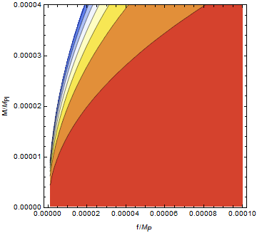
Figure 2: Scalar spectral index as a function parameter $f$ and mass scale $M$.

In fact, even if one were to keep the potential, the contribution at $\epsilon_{1}=1$ would be $\dot{\phi}=-\frac{m_{\alpha}^{2}\phi}{4H}$ and since $H\gg m_{\alpha}$ initially, the kinetic term becomes inferior at that point. This is in the antipode of the result obtained in Ref. [71], and this behavior occurs only because the continuity equation can be solved algebraically with respect to $\dot{\phi}$ in the case at hand, due to the inclusion of the Gauss-Bonnet density and the constraint (6). We shall leave this issue for the time being and focus on the inflationary era only.

Since $\dot{\phi}$ has been extracted, a simple designation of the free parameters of the model suffices in order to derive results. In particular, since the Hubble rate expansion in the first horizon crossing is given by the relation,

$$\centering H=\frac{M}{\sqrt{6}}\sqrt{2N+1}\,,\@add@centering$$ (30)

we find that,

$$\centering\dot{\phi}=-\frac{2M^{3}(N+\frac{1}{2})^{\frac{3}{2}}}{f\sqrt{3}}\,,\@add@centering$$ (31)

therefore parameters $x$ $y$, $\epsilon_{i}$ and in consequence the observed indices are completely specified by $N$, $f$ and $M$. From a numerical standpoint, for $N=60$, $M=1.25\times 10^{-5}M_{P}$ and $f=10^{-5}M_{P}$, one finds that $n_{\mathcal{S}}=0.96686$, $n_{\mathcal{T}}=-0.000413283$ and $r=0.00327847$ which is in agreement with the latest Planck data [112]. As expected, the results do not differ so much from the vacuum $R^{2}$ model exactly because string corrections and the scalar field were assumed to be inferior to the $f(R)$ part. This can also be seen in Fig. 3 where we confront the linear model at hand with the latest Planck likelihood curves and the pure $R^{2}$ model results are also included.

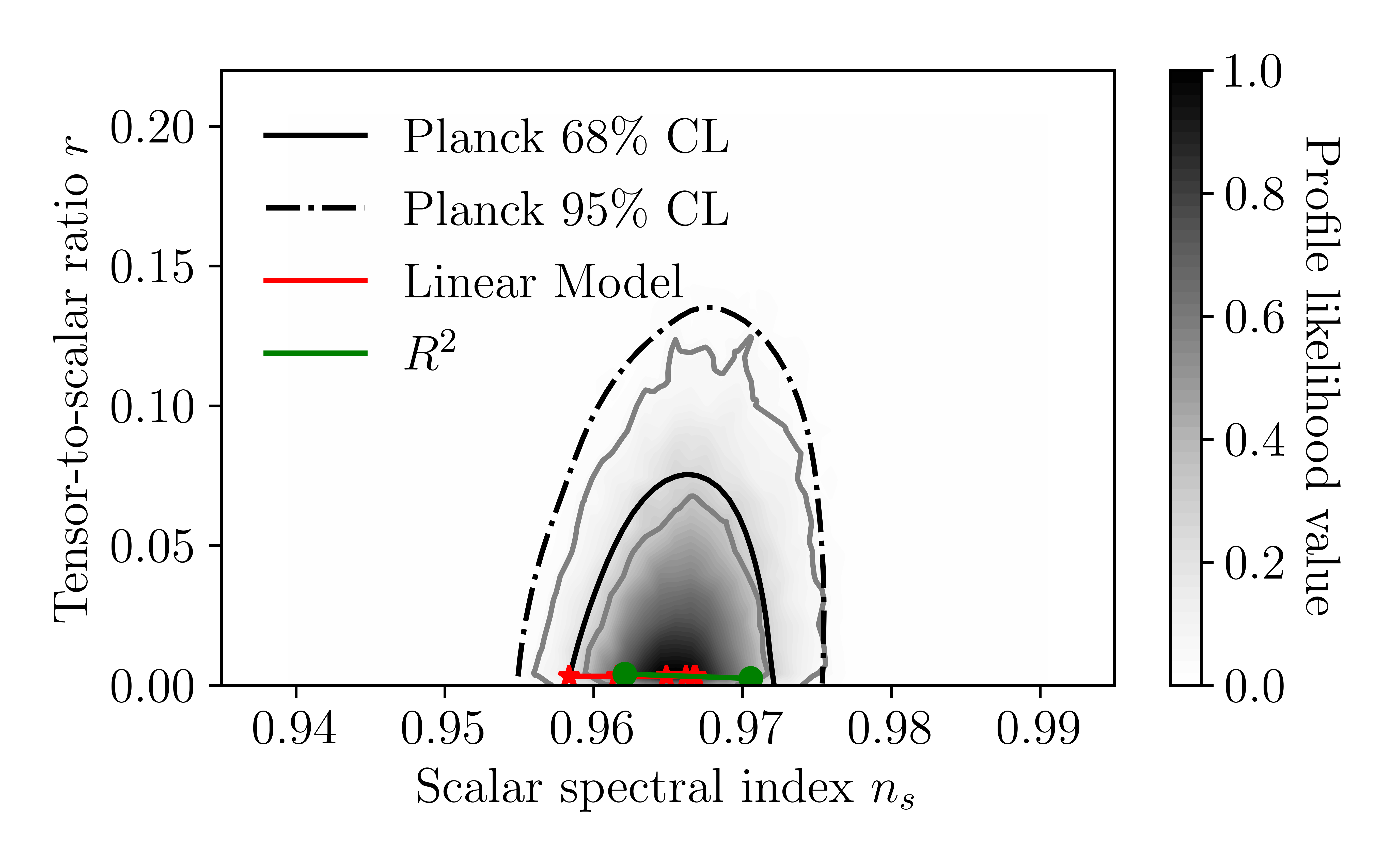
Figure 3: Comparison of the linear non-minimal Gauss-Bonnet coupling model to the $R^{2}$ model and the latest Planck likelihood curves.

This can be inferred from the numerical values of $x$ and $y$ which read $7\times 10^{-9}$ and $3\times 10^{-8}$ respectively, therefore neglecting the kinetic term and the string corrections in the background equations, this is justified. It is also interesting to mention that the above results are independent of the initial value $\phi_{i}$ of the scalar field, and thus the results are valid for a plethora of values for $\phi_{i}$ and $f_{\alpha}$. The only condition in order for the approximation in (9) to be valid is to demand that $\phi_{i}\leq\frac{f_{\alpha}}{10}$, therefore if $f$ in the above model is identified as the axion decay constant such that $f_{\alpha}\sim\mathcal{O}(10^{13})$GeV then $\phi_{i}\leq\mathcal{O}(10^{12})$GeV. According to Fig. 2, $f$ cannot be decreased any further since the scalar spectral index becomes incompatible with observations.

As a final note, it should be mentioned that the constant-roll condition for the scalar field $\ddot{\phi}=H\dot{\phi}$, due to the constraint on the propagation velocity of tensor perturbations, is connected to the production of scalar non-Gaussianities in the CMB. In principle, a detailed analysis should be made however, due to the fact that the $f(R)$ part dominates, one can expect that no matter the numerical value of index $\epsilon_{2}$ during the first horizon crossing where $k=Ha$, the equilateral nonlinear term $f_{NL}^{eq}$ should be at leading order approximately equal to [113]

$$\centering f_{NL}^{eq}=\frac{5}{12}(1-n_{\mathcal{S}})\,,\@add@centering$$ (32)

where according to the previous results, it should be approximately of order $\mathcal{O}(10^{-2})$. Overall, the kinetic axion scalar field cannot enhance the vacuum $R^{2}$ result, as it is subleading.

Now the novel outcome of this model is that the kinetic axion mechanism for the string-corrected $R^{2}$ gravity model does not produce a kination era after the end of inflation. As we showed, the condition $\dot{\phi}\sim 0$ is imposed by the physics of the problem in the case at hand, therefore at the end of inflation, the effective equation of state of the axion is basically a nearly de-Sitter slightly turned to quintessential one. Now the physics in this scenario could be interesting, since the Universe may be overwhelmed by an early dark energy era caused by the kinetic axion which behaves as a slow-roll scalar at the end of inflation. This behavior is entirely caused by the extra Gauss-Bonnet term. One thing is certain for sure, the axion oscillations must be significantly delayed in this model, since the condition $\dot{\phi}\simeq 0$ clearly indicates that the evolution of the axion down to the minimum of its potential is delayed, and the axion slowly-rolls down to its minimum in a modulated way controlled by the Gauss-Bonnet coupling. The axion in this scenario is not driving the initial inflationary era, but it seems that it may control the post-$f(R)$ gravity inflation cosmological era. The vacuum fluctuations of the $R^{2}$ term may not be able to initiate the reheating era. Therefore, what we may are facing in this case is basically a second short slow-roll era controlled by the axion prior the Hubble rate reaches the value $m_{a}\sim H$. It is thus a physical situation where the $R^{2}$ fluctuations are competing a slow-roll axion, but there is a caveat in this scenario, mainly the fact that the energy density of the axion $\rho_{a}\sim a^{-3(1+w)}$ for a nearly de-Sitter era is almost constant $\rho_{a}\sim\mathrm{const}$, while in the kinetic axion case $\rho_{a}\sim a^{-6}$ and for a purely matter dominated post-inflationary era $\rho_{a}\sim a^{-3}$. Hence, it is apparent that the contribution of the axion to the $R^{2}$ reheating process is comparable to $\kappa^{2}\rho_{a}\sim\kappa^{2}$ thus the standard $R^{2}$ reheating occurs. In this case however, the axion oscillations are somewhat delayed, but slightly.

III.2 The Choice of an Exponential non-minimal Gauss-Bonnet Coupling Function

The second model that shall be discussed is the case in which the Gauss-Bonnet coupling has an exponential form,

$$\centering\xi(\phi)=\mathrm{e}^{-\frac{\phi}{f}}\,.\@add@centering$$ (33)

This model was studied in Ref. [108] and as it was shown, the exponential model resulted, depending on the value of $f$, to either eternal or no inflation at all. Therefore, it is intriguing to study the exponential model in this case in order to examine under which circumstances it can result to a viable inflationary era. Now, since the Gauss-Bonnet coupling is not linear, the following set of equations need to be used,

$$\centering\dot{\phi}\@add@centering =\frac{2H\xi^{\prime}}{\xi^{\prime\prime}}\bigg{[}1-\sqrt{1+6\xi^{\prime\prime}H^{2}(1-\epsilon_{1})}\bigg{]}\,, \epsilon_{2} =-1+2\sqrt{1+6\xi^{\prime\prime}H^{2}(1-\epsilon_{1})}\,,$$ (34)

where due to the fact that the factor $1-\epsilon_{1}$ appears, the time derivative at the end of inflation is identically equal to zero. Similarly as in the previous case, this outcome suggests that the kinetic term is not dominant compared to the potential, therefore the intermediate stiff matter era that emerged in Ref. [71] is avoided in this model too. In other words, the inclusion of the Gauss-Bonnet density in Eq. (4) suggests that it cannot result in a reduction of the tensor-to-scalar ratio due to the fact that the inflationary era cannot be prolonged any further. Even if the potential is present in the continuity equation, then the solution of (12) accounting for the constraint (6) suggests that,

$$\centering\dot{\phi}=\frac{2H\xi^{\prime}}{\xi^{\prime\prime}}\bigg{[}1-\sqrt{1+6H^{2}\xi^{\prime\prime}(1-\epsilon_{1})+\frac{V^{\prime}\xi^{\prime\prime}}{4\xi^{\prime}H^{2}}}\bigg{]}\,,\@add@centering$$ (35)

therefore for $\epsilon_{1}=1$, one can see that the ratio between the kinetic term and the scalar potential of the axion is,

$$\centering\frac{\dot{\phi}^{2}}{2V}=\bigg{(}\frac{2\xi^{\prime}}{\xi^{\prime\prime}\phi}\bigg{)}^{2}\bigg{(}\frac{H}{m_{\alpha}}\bigg{)}^{2}\bigg{[}1-\sqrt{1+\frac{\phi\xi^{\prime\prime}}{4\xi^{\prime}}\bigg{(}\frac{m_{\alpha}}{H}\bigg{)}^{2}}\bigg{]}^{2}\,.\@add@centering$$ (36)

Provided that at the end of inflation, $\frac{H}{m_{\alpha}}\gg 1$, then by performing a Taylor expansion one finds that,

$$\centering\frac{\dot{\phi}^{2}}{2V}\simeq\bigg{(}\frac{m_{\alpha}}{4H}\bigg{)}^{2}\,,\@add@centering$$ (37)

and thus, the kinetic term is inferior therefore the model does not predict any increase in the duration of inflation, exactly as was the case with the linear Gauss-Bonnet coupling. Therefore, this result is the same regardless of the coupling chosen.

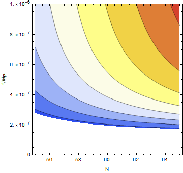
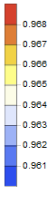
Figure 4: Spectral index $n_{\mathcal{S}}$ depending on parameters $f$ and $N$ on the left and $f$ and $M$ on the right.

Let us now proceed with the numerical results of the model at hand. By using similar values as in the linear coupling such as $N=60$ and $M=1.25\times 10^{-5}M_{P}$, for the case of $f=10^{-6}M_{P}$ and $\phi_{i}=10^{-10}M_{P}$ one finds that $n_{\mathcal{S}}=0.965791$, $n_{\mathcal{T}}=-0.000413309$ and $r=0.00327848$ which are obviously in agreement with Planck data. As expected, since $x=1.5\times 10^{-10}$ and $y=4\times 10^{-8}$, the scalar field is subleading in background equations and the tensor spectral index and tensor-to-scalar ratio are equivalent to their vacuum $R^{2}$ counterparts and only the scalar spectral index is affected to some degree, due to the small value of $f$. It should be stated that such value increases extremely the second and fourth index as now $\epsilon_{2}=273.994$ and $\epsilon_{4}=-274.001$ however in order to have correct results, we are interested in their sum and their slow-variation as it was mentioned previously. Obviously, larger values of $f$ decrease the aforementioned indices but do not influence the scalar spectral index, see Fig.4 for further details on the scalar spectral index. Finally, since the initial value of the scalar field was assumed to be approximately $\phi_{i}\sim\mathcal{O}(10^{8})$ GeV, the approximation on the canonical potential (9) applies if the axion decay constant is $f_{\alpha}\geq\mathcal{O}(10^{9})$GeV.

As a general note, the inclusion of additional string terms does not seem to influence the overall phenomenology. A back-of-the-envelope calculation for the case of an additional string correction,

$$\centering\mathcal{S}=\int d^{4}x\sqrt{-g}\bigg{(}\frac{f(R)}{2\kappa^{2}}-\frac{1}{2}g^{\mu\nu}\nabla_{\mu}\phi\nabla_{\nu}\phi-V(\phi)-\xi(\phi)\bigg{(}\mathcal{G}+cG^{\mu\nu}\nabla_{\mu}\phi\nabla_{\nu}\phi\bigg{)}\bigg{)}\,,\@add@centering$$ (38)

that also affects tensor perturbations suggests that if the constraint $c_{\mathcal{T}}^{2}=1$ is once again imposed such that $\ddot{\xi}=H\dot{\xi}-\frac{c\xi\dot{\phi}^{2}}{4}$, the numerical results are not affected for similar set of values for the free parameters and $\dot{\phi}^{2}(t_{end})\ll V_{end}$ once again.

IV Phase Space Analysis of the Model

In the last section of this paper we shall briefly discuss the phase space of the proposed kinetic axion $f(R)$ gravity model. By including perfect matter fluids, including radiation and dark matter fluids, the gravitational action reads,

$$\centering\mathcal{S}=\int d^{4}x\sqrt{-g}\bigg{(}\frac{f(R)}{2\kappa^{2}}-\frac{1}{2}g^{\mu\nu}\nabla_{\mu}\phi\nabla_{\nu}\phi-V(\phi)-\xi(\phi)\mathcal{G}+\mathcal{L}_{matter}\bigg{)}\,,\@add@centering$$ (39)

and in consequence, the background equations (10) and (11) are rewritten as,

$$\centering\frac{3FH^{2}}{\kappa^{2}}=\rho+\frac{FR-f}{2\kappa^{2}}-\frac{3H\dot{F}}{\kappa^{2}}+\frac{1}{2}\dot{\phi}^{2}+V\,,\@add@centering$$ (40)

$$\centering-\frac{2F\dot{H}}{\kappa^{2}}=\rho+P+\frac{\ddot{F}-H\dot{F}}{\kappa^{2}}+\dot{\phi}^{2}\,,\@add@centering$$ (41)

where $\rho$ and $P$ are the total energy density and pressure of the perfect matter fluids respectively. With regard to the latter, we shall assume that the axion is the sole dark matter component and that other extra dark matter components are not present. In order to perform an autonomous dynamical analysis, the Gauss-Bonnet scalar coupling function shall remain unspecified and the rest functions of the model will follow a power-law form,

$$\centering f(R)\@add@centering =R+AR^{n}\,, V(\phi) =V_{0}(\kappa\phi)^{m}\,,$$ (42)

for the sake of generality however we shall limit our results in the case of $n=2=m$ where in turn $A=\frac{1}{6M^{2}}$ and $V_{0}=\frac{m_{\alpha}^{2}}{2\kappa^{2}}$. In addition, let us define the following dynamical variables,

$$\centering x\@add@centering =\frac{\kappa^{2}\dot{\phi}^{2}}{6FH^{2}}\,, y =\frac{\kappa^{2}V}{3FH^{2}}\,, z =\frac{8\kappa^{2}\dot{\xi}H}{F}\,, u =-\frac{\dot{F}}{HF}\,, v =-\frac{f}{6FH^{2}}\,, w =\frac{R}{6H^{2}}\,, s =\frac{\dot{V}}{HV}\,, p =\frac{\kappa^{2}\rho_{r}}{3FH^{2}}\,, q =\frac{\kappa^{2}\rho_{m}}{3FH^{2}}\,,$$ (43)

where $p$ and $q$ should not be mistaken with $\Omega_{r}$ and $\Omega_{m}$ due to the $F$ part in the denominator. In consequence, equations (40) and (12) are rewritten as,

$$\centering x+y+z+u+v+w+p+q=1\,,\@add@centering$$ (44)

$$\centering\frac{\ddot{\phi}}{H\dot{\phi}}=-3-\frac{s}{2}\frac{y}{x}-\frac{z}{2x}(w-1)\,.\@add@centering$$ (45)

Now by making use of the $e$-foldings number through the differential equation $\frac{d}{dN}=\frac{1}{H}\frac{d}{dt}$, the following set of differential equations is produced,

$$\centering\frac{dx}{dN}=x\bigg{[}-6-\frac{y}{x}-\frac{z}{x}(w-1)+u-2(w-2)\bigg{]}\,,\@add@centering$$ (46)

$$\centering\frac{dy}{dN}=y\bigg{[}s+u-2(w-2)\bigg{]}\,,\@add@centering$$ (47)

$$\centering\frac{dz}{dN}=z\bigg{[}w-1+u\bigg{]}\,,\@add@centering$$ (48)

$$\centering\frac{du}{dN}=u(u+1)+6x+4p+3q+2(w-2)(1-z-\frac{u}{2})\,,\@add@centering$$ (49)

$$\centering\frac{dv}{dN}=v(u-2(w-2))+\frac{uw^{2}}{n(v+w)}\,,\@add@centering$$ (50)

$$\centering\frac{dw}{dN}=-w\bigg{[}\frac{uw}{n(v+w)}+2(w-2)\bigg{]}\,,\@add@centering$$ (51)

$$\centering\frac{ds}{dN}=s\bigg{[}-3-\frac{s}{2}\frac{y}{x}-\frac{z}{2x}(w-1)-(u-2)-\frac{s}{m}\bigg{]}\,,\@add@centering$$ (52)

$$\centering\frac{dp}{dN}=p(u-2w)\,,\@add@centering$$ (53)

$$\centering\frac{dq}{dN}=q(u-2w+1)\,.\@add@centering$$ (54)

Let us study two separate cases. Firstly, we focus on the vacuum $R^{2}$ kinetic axion model, therefore the parameters $y$ and $s$ are neglected along with $p$ and $q$. Therefore, a subsystem comprised of variables $x$ and $z$, that are connected to the axion dynamics and the Gauss-Bonnet term, along with $u$, $v$ and $w$, connected to the $f(R)$ part, is studied. This subsystem can be solved relatively straightforward. So as expected, the inclusion of the Gauss-Bonnet produces a richer phase space. As presented in Table 1, there exist four fixed points in total, one of them being a de Sitter fixed point, another is connected to matter while additionally a third to radiation domination eras and finally, the new stable fixed point from the Gauss-Bonnet contribution describes acceleration and since $\omega_{eff}=-1.6667$, it predicts a phantom evolution. This is the case of phantom dark energy that has been covered in Ref. [114].

Fixed Point	$(x,z,u,v,w)$	Eigenvalues	Stability	q	$\omega_{eff}$
$P_{1}$	(0,0,-4,5,0)	(-6,-5,-5,4,0)	Non Hyperbolic	1	$\frac{1}{3}$
$P_{2}$	(0,0,0,-1,0)	(0,-6,1,-3,0)	Non Hyperbolic	-1	-1
$P_{3}$	($-\frac{9}{4}$,0,3,-$\frac{1}{4}$,$\frac{1}{2}$)	(6,3,3,$\frac{5}{2}$,-$\frac{3}{2}$)	Saddle	$\frac{1}{2}$	0
$P_{4}$	($-\frac{3}{8}$,-$\frac{15}{16}$,-2,-$\frac{3}{2}$,3)	(-9.42318,-5.74568,-4,-2,-0.831139)	Stable Node	-2	-$\frac{5}{3}$

Table 1: Fixed points for the vacuum model with subleading potential.

Now if one includes the potential, along with variable $s$, it turns out that no additional fixed point emerges since $y\to 0$ and only $s$ can obtain a non-zero but finite value. This however does not affect the Friedmann constraint neither the stability of the fixed points, it only suggests how $y$ or in other words $\phi$ evolves. Finally, the inclusion of perfect matter fluids increases the number of fixed points by two, as shown in Table 2 and surprisingly, these fixed points have nothing to do with matter or radiation. In fact, the first fixed point is connected to a static universe as $\omega_{eff}=-\frac{1}{3}$ whereas the second describes quintessential acceleration with $\omega_{eff}=-\frac{1}{2}$. In a sense, the $f(R)$ gravity describes both de-Sitter and radiation domination eras, while the kinetic term of the axion describes matter domination. This is somewhat expected since the axion is a dark matter component.

Fixed Point	$(x,y,z,u,v,w,p,q)$	Eigenvalues	Stability	q	$\omega_{eff}$
$P_{1}$	(0,0,0,-4,5,0,0,0)	(-6,-5,-5,4,4,-3,0,0)	Non Hyperbolic	1	$\frac{1}{3}$
$P_{2}$	(0,0,0,0,-1,0,0,0)	(0,0,-6,-4,-3,1,-3,0)	Non Hyperbolic	-1	-1
$P_{3}$	($-\frac{9}{4}$,0,0,3,-$\frac{1}{4}$,$\frac{1}{2},0,0$)	(6,6,3,3,3,$\frac{5}{2}$,2,-$\frac{3}{2}$)	Saddle	$\frac{1}{2}$	0
$P_{4}$	($-\frac{3}{8}$,0,-$\frac{15}{16}$,-2,-$\frac{3}{2}$,3,0,0)	(-9.42318,-8,-7,-5.74568,-4,-4,-2,-0.831139)	Stable Node	-2	-$\frac{5}{3}$
$P_{5}$	(0,0,2,-$\frac{1}{2}$,1,0,-$\frac{3}{2}$,0 )	(4,4,-2.44949,2.44949,-2,2,2,1 )	Saddle	0	$-\frac{1}{3}$
$P_{6}$	(0,0,$\frac{3}{2}$,-$\frac{5}{8}$,$\frac{5}{4}$0,0,-$\frac{9}{8}$ )	( -3,3,3,-2.77617,2.02617,1.75,1.5,-1)	Saddle	$-\frac{1}{4}$	$-\frac{1}{2}$

Table 2: Fixed point of the complete model.

As a final note, it should be stated that under the assumption that $c_{\mathcal{T}}^{2}=1$, the constraint in Eq. (7) should be implemented in the continuity equation of the scalar field as well. In consequence, if it is combined with Eq. (45), an additional equation emerges that needs to be satisfied at all times and reads,

$$\centering 2(4-\lambda)x+sy+z(w-1)=0\,,\@add@centering$$ (55)

where $\lambda=\frac{\dot{\xi}^{\prime}}{H\xi^{\prime}}$ is an additional auxiliary parameter. This condition is respected by the fixed points which were previously derived and for a nonzero but finite value of $x$, which was shown to manifest previously, parameter $\lambda$ simply obtains a specific value. The linear Gauss-Bonnet coupling is a special case since it suggests that $\lambda=0$ identically therefore the fixed points $P_{3}$ through $P_{6}$ cannot satisfy the aforementioned constraint.

We need to note that in principle, in the context of our model, it is possible to satisfy in a concrete way all the Swampland criteria, due to the freedom offered by the $f(R)$ sector and the Gauss-Bonnet coupling, something which is not possible in ordinary scalar field theories [115, 116, 117].

V Conclusions

In this work we studied the effects of a non-minimal coupling of the kinetic misalignment axion field on the inflationary era generated by an $R^{2}$ gravity. In the case of kinetic axion $R^{2}$ gravity, the inflationary controlled by the $R^{2}$ gravity is somewhat prolonged by the kinetic axion, since at the end of inflation, the stiff axion evolution prevails the evolution, thus the reheating era is delayed. This is due to the fact that the kinetic axion at the end of the inflationary era dominates over the $R^{2}$ fluctuations which would start the reheating process, and in effect, the background equation of state parameter would have value $w=1$. In turn, this affects the total number of the $e$-foldings and hence the inflationary era is prolonged. Also in the same context, the reheating era is somewhat shortened, thus the Universe in this scenario would have a lower reheating temperature compared to the canonical misalignment axion $R^{2}$ model. However, as we showed in this article, the non-trivial Gauss-Bonnet coupling can have dramatic effects on the axion itself, imposing the condition $\dot{\phi}\simeq 0$ at the end of the inflationary era. In this case it is obvious that the kinetic evolution of the axion is stopped at the end of inflation, and thus the axion reaches the minimum of its potential faster. Therefore, it starts its oscillations around its minimum in a standard way when its mass is of the same order as the Hubble rate, and therefore the $R^{2}$ fluctuations control the reheating era. Thus in some way, the non-trivial Gauss-Bonnet coupling of the axion, counteracts on the kination axion mechanism, eliminating the stiff era axion evolution at the end of the inflationary era. At a phenomenological level, the $R^{2}$-corrected canonical misalignment axion model and the kinetic axion $R^{2}$ inflation model with Gauss-Bonnet corrections are almost indistinguishable.

References

- [1] G. Bertone, D. Hooper and J. Silk, Phys. Rept. 405 (2005) 279 doi:10.1016/j.physrep.2004.08.031 [hep-ph/0404175].
- [2] L. Bergstrom, Rept. Prog. Phys. 63 (2000) 793 doi:10.1088/0034-4885/63/5/2r3 [hep-ph/0002126].
- [3] Y. Mambrini, S. Profumo and F. S. Queiroz, Phys. Lett. B 760 (2016) 807 [arXiv:1508.06635 [hep-ph]].
- [4] S. Profumo, arXiv:1301.0952 [hep-ph].
- [5] D. Hooper and S. Profumo, Phys. Rept. 453 (2007) 29 [hep-ph/0701197].
- [6] V. K. Oikonomou, J. D. Vergados and C. C. Moustakidis, Nucl. Phys. B 773 (2007) 19 [hep-ph/0612293].
- [7] J. Preskill, M. B. Wise and F. Wilczek, Phys. Lett. 120B (1983) 127. doi:10.1016/0370-2693(83)90637-8
- [8] L. F. Abbott and P. Sikivie, Phys. Lett. 120B (1983) 133. doi:10.1016/0370-2693(83)90638-X
- [9] M. Dine and W. Fischler, Phys. Lett. 120B (1983) 137. doi:10.1016/0370-2693(83)90639-1
- [10] D. J. E. Marsh, Phys. Rept. 643 (2016) 1 [arXiv:1510.07633 [astro-ph.CO]].
- [11] F. Chadha-Day, J. Ellis and D. J. E. Marsh, Sci. Adv. 8 (2022) no.8, abj3618 doi:10.1126/sciadv.abj3618 [arXiv:2105.01406 [hep-ph]].
- [12] K. Choi, S. H. Im and C. Sub Shin, Ann. Rev. Nucl. Part. Sci. 71 (2021), 225-252 doi:10.1146/annurev-nucl-120720-031147 [arXiv:2012.05029 [hep-ph]].
- [13] L. Di Luzio, M. Giannotti, E. Nardi and L. Visinelli, Phys. Rept. 870 (2020), 1-117 doi:10.1016/j.physrep.2020.06.002 [arXiv:2003.01100 [hep-ph]].
- [14] P. Sikivie, Lect. Notes Phys. 741 (2008) 19 [astro-ph/0610440].
- [15] G. G. Raffelt, Lect. Notes Phys. 741 (2008) 51 [hep-ph/0611350].
- [16] A. D. Linde, Phys. Lett. B 259 (1991) 38.
- [17] R. T. Co, L. J. Hall and K. Harigaya, Phys. Rev. Lett. 124 (2020) no.25, 251802 doi:10.1103/PhysRevLett.124.251802 [arXiv:1910.14152 [hep-ph]].
- [18] R. T. Co, L. J. Hall, K. Harigaya, K. A. Olive and S. Verner, JCAP 08 (2020), 036 doi:10.1088/1475-7516/2020/08/036 [arXiv:2004.00629 [hep-ph]].
- [19] B. Barman, N. Bernal, N. Ramberg and L. Visinelli, [arXiv:2111.03677 [hep-ph]].
- [20] M. C. D. Marsh, H. R. Russell, A. C. Fabian, B. P. McNamara, P. Nulsen and C. S. Reynolds, JCAP 1712 (2017) no.12, 036 [arXiv:1703.07354 [hep-ph]].
- [21] S. D. Odintsov and V. K. Oikonomou, Phys. Rev. D 99 (2019) no.6, 064049 [arXiv:1901.05363 [gr-qc]].
- [22] S. Nojiri, S. D. Odintsov, V. K. Oikonomou and A. A. Popov, Phys. Rev. D 100 (2019) no.8, 084009 [arXiv:1909.01324 [gr-qc]].
- [23] S. Nojiri, S. D. Odintsov and V. K. Oikonomou, Annals Phys. 418 (2020), 168186 doi:10.1016/j.aop.2020.168186 [arXiv:1907.01625 [gr-qc]].
- [24] S. D. Odintsov and V. K. Oikonomou, Phys. Rev. D 99 (2019) no.10, 104070 [arXiv:1905.03496 [gr-qc]].
- [25] M. Cicoli, V. Guidetti and F. G. Pedro, arXiv:1903.01497 [hep-th].
- [26] H. Fukunaga, N. Kitajima and Y. Urakawa, arXiv:1903.02119 [astro-ph.CO].
- [27] A. Caputo, arXiv:1902.02666 [hep-ph].
- [28] A.S.Sakharov and M.Yu.Khlopov, Yadernaya Fizika (1994) V. 57, PP. 514- 516. ( Phys.Atom.Nucl. (1994) V. 57, PP. 485-487); A.S.Sakharov, D.D.Sokoloff and M.Yu.Khlopov, Yadernaya Fizika (1996) V. 59, PP. 1050-1055. (Phys.Atom.Nucl. (1996) V. 59, PP. 1005-1010); M .Yu.Khlopov, A.S.Sakharov and D.D.Sokoloff, Nucl.Phys. B (Proc. Suppl.) (1999) V. 72, 105-109.
- [29] J. H. Chang, R. Essig and S. D. McDermott, JHEP 1809 (2018) 051 [arXiv:1803.00993 [hep-ph]]. Chang:2018rso,Irastorza:2018dyq,
- [30] I. G. Irastorza and J. Redondo, Prog. Part. Nucl. Phys. 102 (2018) 89 [arXiv:1801.08127 [hep-ph]].
- [31] V. Anastassopoulos et al. [CAST Collaboration], Nature Phys. 13 (2017) 584 [arXiv:1705.02290 [hep-ex]].
- [32] P. Sikivie, Phys. Rev. Lett. 113 (2014) no.20, 201301 [arXiv:1409.2806 [hep-ph]].
- [33] P. Sikivie, Phys. Lett. B 695 (2011) 22 [arXiv:1003.2426 [astro-ph.GA]].
- [34] P. Sikivie and Q. Yang, Phys. Rev. Lett. 103 (2009) 111301 [arXiv:0901.1106 [hep-ph]].
- [35] A. Caputo, L. Sberna, M. Frias, D. Blas, P. Pani, L. Shao and W. Yan, Phys. Rev. D 100 (2019) no.6, 063515 [arXiv:1902.02695 [astro-ph.CO]].
- [36] E. Masaki, A. Aoki and J. Soda, arXiv:1909.11470 [hep-ph].
- [37] J. Soda and D. Yoshida, Galaxies 5 (2017) no.4, 96.
- [38] J. Soda and Y. Urakawa, Eur. Phys. J. C 78 (2018) no.9, 779 [arXiv:1710.00305 [astro-ph.CO]].
- [39] A. Aoki and J. Soda, Phys. Rev. D 96 (2017) no.2, 023534 [arXiv:1703.03589 [astro-ph.CO]].
- [40] E. Masaki, A. Aoki and J. Soda, Phys. Rev. D 96 (2017) no.4, 043519 [arXiv:1702.08843 [astro-ph.CO]].
- [41] A. Aoki and J. Soda, Int. J. Mod. Phys. D 26 (2016) no.07, 1750063 [arXiv:1608.05933 [astro-ph.CO]].
- [42] I. Obata and J. Soda, Phys. Rev. D 94 (2016) no.4, 044062 [arXiv:1607.01847 [astro-ph.CO]].
- [43] A. Aoki and J. Soda, Phys. Rev. D 93 (2016) no.8, 083503 [arXiv:1601.03904 [hep-ph]].
- [44] T. Ikeda, R. Brito and V. Cardoso, Phys. Rev. Lett. 122 (2019) no.8, 081101 [arXiv:1811.04950 [gr-qc]].
- [45] A. Arvanitaki, S. Dimopoulos, M. Galanis, L. Lehner, J. O. Thompson and K. Van Tilburg, arXiv:1909.11665 [astro-ph.CO].
- [46] A. Arvanitaki, M. Baryakhtar, S. Dimopoulos, S. Dubovsky and R. Lasenby, Phys. Rev. D 95 (2017) no.4, 043001 [arXiv:1604.03958 [hep-ph]].
- [47] A. Arvanitaki, M. Baryakhtar and X. Huang, Phys. Rev. D 91 (2015) no.8, 084011 [arXiv:1411.2263 [hep-ph]].
- [48] A. Arvanitaki and A. A. Geraci, Phys. Rev. Lett. 113 (2014) no.16, 161801 [arXiv:1403.1290 [hep-ph]].
- [49] S. Sen, Phys. Rev. D 98 (2018) no.10, 103012 [arXiv:1805.06471 [hep-ph]].
- [50] V. Cardoso, S. J. C. Dias, G. S. Hartnett, M. Middleton, P. Pani and J. E. Santos, JCAP 1803 (2018) 043 [arXiv:1801.01420 [gr-qc]].
- [51] J. G. Rosa and T. W. Kephart, Phys. Rev. Lett. 120 (2018) no.23, 231102 [arXiv:1709.06581 [gr-qc]].
- [52] H. Yoshino and H. Kodama, PTEP 2014 (2014) 043E02 [arXiv:1312.2326 [gr-qc]].
- [53] C. S. Machado, W. Ratzinger, P. Schwaller and B. A. Stefanek, arXiv:1912.01007 [hep-ph].
- [54] A. Korochkin, A. Neronov and D. Semikoz, arXiv:1911.13291 [hep-ph].
- [55] A. S. Chou, Astrophys. Space Sci. Proc. 56 (2019) 41.
- [56] C. F. Chang and Y. Cui, arXiv:1911.11885 [hep-ph].
- [57] N. Crisosto, G. Rybka, P. Sikivie, N. S. Sullivan, D. B. Tanner and J. Yang, arXiv:1911.05772 [astro-ph.CO].
- [58] K. Choi, H. Seong and S. Yun, arXiv:1911.00532 [hep-ph].
- [59] M. Kavic, S. L. Liebling, M. Lippert and J. H. Simonetti, arXiv:1910.06977 [astro-ph.HE].
- [60] D. Blas, A. Caputo, M. M. Ivanov and L. Sberna, arXiv:1910.06128 [hep-ph].
- [61] D. Guerra, C. F. B. Macedo and P. Pani, JCAP 1909 (2019) no.09, 061 [arXiv:1909.05515 [gr-qc]].
- [62] T. Tenkanen and L. Visinelli, JCAP 1908 (2019) 033 [arXiv:1906.11837 [astro-ph.CO]].
- [63] G. Y. Huang and S. Zhou, Phys. Rev. D 100 (2019) no.3, 035010 [arXiv:1905.00367 [hep-ph]].
- [64] D. Croon, R. Houtz and V. Sanz, JHEP 1907 (2019) 146 [arXiv:1904.10967 [hep-ph]].
- [65] F. V. Day and J. I. McDonald, JCAP 1910 (2019) no.10, 051 [arXiv:1904.08341 [hep-ph]].
- [66] S. D. Odintsov and V. K. Oikonomou, EPL 129 (2020) no.4, 40001 doi:10.1209/0295-5075/129/40001 [arXiv:2003.06671 [gr-qc]].
- [67] S. Nojiri, S. D. Odintsov, V. K. Oikonomou and A. A. Popov, Phys. Dark Univ. 28 (2020), 100514 doi:10.1016/j.dark.2020.100514 [arXiv:2002.10402 [gr-qc]].
- [68] S. D. Odintsov and V. K. Oikonomou, Phys. Rev. D 101 (2020) no.4, 044009 doi:10.1103/PhysRevD.101.044009 [arXiv:2001.06830 [gr-qc]].
- [69] V. K. Oikonomou, Phys. Rev. D 103 (2021) no.4, 044036 doi:10.1103/PhysRevD.103.044036 [arXiv:2012.00586 [astro-ph.CO]].
- [70] V. K. Oikonomou, EPL 139 (2022) no.6, 69004 doi:10.1209/0295-5075/ac8fb2 [arXiv:2209.08339 [hep-ph]].
- [71] V. K. Oikonomou, Phys. Rev. D 106 (2022) no.4, 044041 doi:10.1103/PhysRevD.106.044041 [arXiv:2208.05544 [gr-qc]].
- [72] K. Mazde and L. Visinelli, JCAP 01 (2023), 021 doi:10.1088/1475-7516/2023/01/021 [arXiv:2209.14307 [astro-ph.CO]].
- [73] Y. Chen, R. Roy, S. Vagnozzi and L. Visinelli, Phys. Rev. D 106 (2022) no.4, 043021 doi:10.1103/PhysRevD.106.043021 [arXiv:2205.06238 [astro-ph.HE]].
- [74] L. Caloni, M. Gerbino, M. Lattanzi and L. Visinelli, JCAP 09 (2022), 021 doi:10.1088/1475-7516/2022/09/021 [arXiv:2205.01637 [astro-ph.CO]].
- [75] R. Roy, S. Vagnozzi and L. Visinelli, Phys. Rev. D 105 (2022) no.8, 083002 doi:10.1103/PhysRevD.105.083002 [arXiv:2112.06932 [astro-ph.HE]].
- [76] L. Di Luzio, J. Galan, M. Giannotti, I. G. Irastorza, J. Jaeckel, A. Lindner, J. Ruz, U. Schneekloth, L. Sohl and L. J. Thormaehlen, et al. Eur. Phys. J. C 82 (2022) no.2, 120 doi:10.1140/epjc/s10052-022-10061-1 [arXiv:2111.06407 [hep-ph]].
- [77] G. Choi, W. Lin, L. Visinelli and T. T. Yanagida, Phys. Rev. D 104 (2021) no.10, 10 doi:10.1103/PhysRevD.104.L101302 [arXiv:2106.12602 [hep-ph]].
- [78] L. Di Luzio, B. Gavela, P. Quilez and A. Ringwald, JHEP 05 (2021), 184 doi:10.1007/JHEP05(2021)184 [arXiv:2102.00012 [hep-ph]].
- [79] M. Bauer, M. Neubert, S. Renner, M. Schnubel and A. Thamm, JHEP 04 (2021), 063 doi:10.1007/JHEP04(2021)063 [arXiv:2012.12272 [hep-ph]].
- [80] N. Ramberg and L. Visinelli, Phys. Rev. D 103 (2021) no.6, 063031 doi:10.1103/PhysRevD.103.063031 [arXiv:2012.06882 [astro-ph.CO]].
- [81] L. Di Luzio, M. Fedele, M. Giannotti, F. Mescia and E. Nardi, Phys. Rev. Lett. 125 (2020) no.13, 131804 doi:10.1103/PhysRevLett.125.131804 [arXiv:2006.12487 [hep-ph]].
- [82] L. Visinelli and S. Vagnozzi, Phys. Rev. D 99 (2019) no.6, 063517 doi:10.1103/PhysRevD.99.063517 [arXiv:1809.06382 [hep-ph]].
- [83] L. Visinelli and J. Redondo, Phys. Rev. D 101 (2020) no.2, 023008 doi:10.1103/PhysRevD.101.023008 [arXiv:1808.01879 [astro-ph.CO]].
- [84] L. Di Luzio, F. Mescia and E. Nardi, Phys. Rev. Lett. 118 (2017) no.3, 031801 doi:10.1103/PhysRevLett.118.031801 [arXiv:1610.07593 [hep-ph]].
- [85] Y. K. Semertzidis and S. Youn, Sci. Adv. 8 (2022) no.8, abm9928 doi:10.1126/sciadv.abm9928 [arXiv:2104.14831 [hep-ph]].
- [86] M. Buschmann, J. W. Foster, A. Hook, A. Peterson, D. E. Willcox, W. Zhang and B. R. Safdi, Nature Commun. 13 (2022) no.1, 1049 doi:10.1038/s41467-022-28669-y [arXiv:2108.05368 [hep-ph]].
- [87] J. Liu et al. [BREAD], Phys. Rev. Lett. 128 (2022) no.13, 131801 doi:10.1103/PhysRevLett.128.131801 [arXiv:2111.12103 [physics.ins-det]].
- [88] S. Hoof and L. Schulz, [arXiv:2212.09764 [hep-ph]].
- [89] H. J. Li and W. Chao, [arXiv:2211.00524 [hep-ph]].
- [90] A. Codello and R. K. Jain, Class. Quant. Grav. 33 (2016) no.22, 225006 doi:10.1088/0264-9381/33/22/225006 [arXiv:1507.06308 [gr-qc]].
- [91] V. K. Oikonomou and I. Giannakoudi, Nucl. Phys. B 978 (2022), 115779 doi:10.1016/j.nuclphysb.2022.115779 [arXiv:2204.02454 [gr-qc]].
- [92] G. Lambiase, L. Mastrototaro and L. Visinelli, JCAP 01 (2023), 011 doi:10.1088/1475-7516/2023/01/011 [arXiv:2207.08067 [hep-ph]].
- [93] S. Nojiri, S. D. Odintsov and V. K. Oikonomou, Phys. Rept. 692 (2017) 1 [arXiv:1705.11098 [gr-qc]].
-
[94]
S. Capozziello, M. De Laurentis,
Phys. Rept. 509, 167 (2011);
- [95] V. Faraoni and S. Capozziello, Fundam. Theor. Phys. 170 (2010).
- [96] S. Nojiri, S.D. Odintsov, Phys. Rept. 505, 59 (2011);
- [97] G. J. Olmo, Int. J. Mod. Phys. D 20 (2011) 413 [arXiv:1101.3864 [gr-qc]].
- [98] S. Nojiri and S. D. Odintsov, Phys. Rev. D 68 (2003) 123512 doi:10.1103/PhysRevD.68.123512 [hep-th/0307288].
- [99] S. Nojiri and S. D. Odintsov, Phys. Lett. B 657 (2007) 238 doi:10.1016/j.physletb.2007.10.027 [arXiv:0707.1941 [hep-th]].
- [100] S. Nojiri and S. D. Odintsov, Phys. Rev. D 77 (2008) 026007 doi:10.1103/PhysRevD.77.026007 [arXiv:0710.1738 [hep-th]].
- [101] G. Cognola, E. Elizalde, S. Nojiri, S. D. Odintsov, L. Sebastiani and S. Zerbini, Phys. Rev. D 77 (2008) 046009 doi:10.1103/PhysRevD.77.046009 [arXiv:0712.4017 [hep-th]].
- [102] S. Nojiri and S. D. Odintsov, Phys. Rev. D 74 (2006) 086005 doi:10.1103/PhysRevD.74.086005 [hep-th/0608008].
- [103] S. A. Appleby and R. A. Battye, Phys. Lett. B 654 (2007) 7 doi:10.1016/j.physletb.2007.08.037 [arXiv:0705.3199 [astro-ph]].
- [104] E. Elizalde, S. Nojiri, S. D. Odintsov, L. Sebastiani and S. Zerbini, Phys. Rev. D 83 (2011) 086006 doi:10.1103/PhysRevD.83.086006 [arXiv:1012.2280 [hep-th]].
- [105] P. M. Sá, Phys. Rev. D 102 (2020) no.10, 103519 doi:10.1103/PhysRevD.102.103519 [arXiv:2007.07109 [gr-qc]].
- [106] W. Y. Ai, Commun. Theor. Phys. 72 (2020) no.9, 095402 doi:10.1088/1572-9494/aba242 [arXiv:2004.02858 [gr-qc]].
- [107] J. c. Hwang and H. Noh, Phys. Rev. D 71 (2005), 063536 doi:10.1103/PhysRevD.71.063536 [arXiv:gr-qc/0412126 [gr-qc]].
- [108] S. D. Odintsov, V. K. Oikonomou and F. P. Fronimos, Nucl. Phys. B 958 (2020), 115135 doi:10.1016/j.nuclphysb.2020.115135 [arXiv:2003.13724 [gr-qc]].
- [109] S. A. Appleby, R. A. Battye and A. A. Starobinsky, JCAP 06 (2010), 005 doi:10.1088/1475-7516/2010/06/005 [arXiv:0909.1737 [astro-ph.CO]].
- [110] V. K. Oikonomou and F. P. Fronimos, EPL 131 (2020) no.3, 30001 doi:10.1209/0295-5075/131/30001 [arXiv:2007.11915 [gr-qc]].
- [111] V. K. Oikonomou, EPL 130 (2020) no.1, 10006 doi:10.1209/0295-5075/130/10006 [arXiv:2004.10778 [gr-qc]].
- [112] N. Aghanim et al. [Planck], Astron. Astrophys. 641 (2020), A6 [erratum: Astron. Astrophys. 652 (2021), C4] doi:10.1051/0004-6361/201833910 [arXiv:1807.06209 [astro-ph.CO]].
- [113] J. M. Maldacena, JHEP 05 (2003), 013 doi:10.1088/1126-6708/2003/05/013 [arXiv:astro-ph/0210603 [astro-ph]].
- [114] R. R. Caldwell, M. Kamionkowski and N. N. Weinberg, Phys. Rev. Lett. 91 (2003), 071301 doi:10.1103/PhysRevLett.91.071301 [arXiv:astro-ph/0302506 [astro-ph]].
- [115] W. H. Kinney, S. Vagnozzi and L. Visinelli, Class. Quant. Grav. 36 (2019) no.11, 117001 doi:10.1088/1361-6382/ab1d87 [arXiv:1808.06424 [astro-ph.CO]].
- [116] A. Kehagias and A. Riotto, Fortsch. Phys. 66 (2018) no.10, 1800052 doi:10.1002/prop.201800052 [arXiv:1807.05445 [hep-th]].
- [117] A. Achúcarro and G. A. Palma, JCAP 02 (2019), 041 doi:10.1088/1475-7516/2019/02/041 [arXiv:1807.04390 [hep-th]].