Practical Cross-System Shilling Attacks with Limited Access to Data

Abstract

In shilling attacks, an adversarial party injects a few fake user profiles into a Recommender System (RS) so that the target item can be promoted or demoted. Although much effort has been devoted to developing shilling attack methods, we find that existing approaches are still far from practical. In this paper, we analyze the properties a practical shilling attack method should have and propose a new concept of Cross-system Attack. With the idea of Cross-system Attack, we design a Practical Cross-system Shilling Attack (PC-Attack) framework that requires little information about the victim RS model and the target RS data for conducting attacks. PC-Attack is trained to capture graph topology knowledge from public RS data in a self-supervised manner. Then, it is fine-tuned on a small portion of target data that is easy to access to construct fake profiles. Extensive experiments have demonstrated the superiority of PC-Attack over state-of-the-art baselines. Our implementation of PC-Attack is available at https://github.com/KDEGroup/PC-Attack.

1 Introduction

Recommender System (RS) has become an essential tool in various online services. However, its prevalence also attracts attackers who try to manipulate RS to mislead users for gaining illegal profits. Among various attacks, Shilling Attack is the most subsistent and profitable one (Lin et al. 2022). RS allows users to interact with the system through various operations such as giving ratings or browsing the page of an item. In shilling attacks, an adversarial party injects a few fake user profiles into the system to hoax RS so that the target item can be promoted or demoted (Gunes et al. 2014). This way, the attacker can increase the possibility that the target item can be viewed/bought by people or impair the competitors by demoting their products. In experiments, shilling attacks are able to spoof real-world RS, including Amazon, YouTube and Yelp (Xing et al. 2013; Yang, Gong, and Cai 2017). In practice, services of various large companies were affected by shilling attacks (Lam and Riedl 2004). Studying how to spoof RS has become a hot direction (Deldjoo, Noia, and Merra 2021) as it gives insights into the defense against malicious attacks.

Although much effort has been devoted to developing new shilling attack methods (Gunes et al. 2014; Deldjoo, Noia, and Merra 2021), we find existing shilling attack approaches are still far from practical. The main reason is that most of them require the complete knowledge of the RS data, which is not available in real shilling attacks. A few works study attacking using incomplete data (Zhang et al. 2021a) or transferring knowledge from other sources to attack the victim RS (Fan et al. 2021). Nevertheless, they still request a large portion of the target data or assume other data sources share some items with the victim RS.

In this paper, we study the problem of designing a practical shilling attack approach. We believe a practical shilling attack method should have the following nice properties:

• Property 1: Do not require any prior knowledge of the victim RS (e.g., model architecture or parameters in the model).

• Property 2: When training the attacker, other data sources (e.g., public RS datasets) instead of the data of the victim RS can be used. Do not assume the training data contain any users or items that exist in the victim RS.

• Property 3: The attacker should use as little information of the data in the victim RS as possible. Required information should be easy to access in practice.

Category	Method	Knowledge			Do not train with a surrogate RS	Do not require multiple queries	Cross-domain attack	Cross-system attack
		Target Data	RS Architecture	RS Parameters
Optimization	PGA and SGLD	$m\cdot n$	✓	✓	✓	✓	×	×
	RevAdv and RAPU	$m\cdot n$	×	×	×	✓	×	×
GAN	TrialAttack	$m\cdot n$	✓	×	×	✓	×	×
	Leg-UP	$m\cdot n$	×	×	×	✓	×	×
	DCGAN, AUSH and RecUP	$m\cdot n$	×	×	✓	✓	×	×
RL	PoisonRec	$e\cdot n\cdot k$	×	×	✓	×	×	×
	LOKI	$m\cdot n$	×	×	×	✓	×	×
	CopyAttack	$e\cdot n\cdot k$	×	×	✓	×	✓	×
KD	Model Extraction Attack	$c\cdot k$	✓	×	✓	×	×	×
	PC-Attack	$p\cdot m\cdot n$	×	×	✓	✓	✓	✓

Table 1: Comparisons of shilling attack approaches. Reference of each method can be found in Sec. 2.1. $m$ and $n$ indicate the numbers of users and items, respectively. $p$ is the maximum percentage of the target data that PC-Attack requires. $e$, $k$ and $c$ represent the number of training epochs, the length of recommendation list and the number of queries, respectively.

Our idea is that limiting the access to the target RS data does not mean that the attacker cannot leverage a large volume of other public RS data to train the attack model. We propose a new concept of Cross-system Attack: Thanks to the prosperous development of RS research, many real RS datasets are available and can be used for extracting knowledge and training the attacker to launch shilling attacks. Along this direction, we design a Practical Cross-system Shilling Attack (PC-Attack) framework that requires little information on the victim RS model and the target RS data. The contributions of this work are summarized as follows:

1. We analyze the inadequacy of existing shilling attack methods and propose the concept of cross-system attack for designing a practical shilling attack model.

2. We design PC-Attack for shilling attacks. PC-Attack is trained to capture graph topology knowledge from public RS data in a self-supervised manner. Then, it is fine-tuned on a small portion of target data that is readily available to construct fake profiles. PC-Attack has all the three nice properties discussed above.

3. We conduct extensive experiments to demonstrate that PC-Attack exceeds state-of-the-art methods w.r.t. attack power and attack invisibility. Even in an unfair comparison where other attack methods can access the complete target data, PC-Attack with limited access to the target data still exhibits superior performance.

2 Background

Shilling attacks can achieve both push attacks (promote the target item) and nuke attacks (demote the target item). Since attackers can easily reverse the goal setting to conduct each attack (Lin et al. 2022), we consider push attacks in the sequel for simplicity. In this paper, the source data and the target data refer to the RS data used for training the attack model and the data in the victim RS, respectively.

2.1 Related Work

Early works of shilling attacks rely on heuristics (Gunes et al. 2014). Recent works (Deldjoo, Noia, and Merra 2021) mostly adopt the idea of adversarial attack (Yuan et al. 2019), and they can be categorized into four groups.

Optimization methods study how to model shilling attacks as an optimization task and then use optimization strategies to solve it. Li et al. (2016) assumes the victim RS adopts matrix factorization (MF) and they propose methods PGA and SGLD that directly add the attack goal into the objective of MF. RevAdv proposed by Tang, Wen, and Wang (2020) and RAPU proposed by Zhang et al. (2021a) model shilling attacks as a bi-level optimization problem.

GAN-based methods adopt Generative Adversarial Network (GAN) (Goodfellow et al. 2014) to construct fake user profiles. The generator models the data distribution of real users and generates real-like data, while the discriminator is responsible for identifying the generated fake users. Along this direction, a large number of methods have sprung up: TrialAttack (Wu et al. 2021), Leg-UP (Lin et al. 2022), DCGAN (Christakopoulou and Banerjee 2019), AUSH (Lin et al. 2020), RecUP (Zhang et al. 2021b), to name a few.

RL-based methods query the RS to get feedback on the attack. Then, Reinforcement Learning (RL) (Kaelbling, Littman, and Moore 1996) is used to adjust the attack. Representative works include PoisonRec (Song et al. 2020), LOKI (Zhang et al. 2020) and CopyAttack (Fan et al. 2021).

KD-based methods leverage Knowledge Distillation (KD) (Gou et al. 2021) to narrow the gap between the surrogate RS and the victim RS. The surrogate RS is used to mimic the victim RS when the prior knowledge is not available. Model Extraction Attack proposed by Yue et al. (2021) falls in this category.

2.2 Analysis of Existing Works

We review existing shilling attack approaches and summarize their characteristics in Tab. 1:

• Data Knowledge: Some methods assume the complete/partial target data is exposed to attackers. A practical attack method should use as less target data as possible.

• RS Parameter Knowledge: Some methods require the knowledge of the learned parameters of the victim RS. Such information is typically not available.

• RS Architecture Knowledge: Some methods require the knowledge of the architecture of the victim RS. Such information is typically not available.

• Train with a surrogate RS: Use a surrogate RS to train the attacker to avoid the prior knowledge of the victim RS.

• Require multiple queries: Query the victim RS multiple times and adjust fake profiles according to the feedback.

• Cross-domain Attack: Use the information in one RS domain to attack another RS domain, e.g., train on the book data in Amazon RS and then attack video items in Amazon RS. Source and target domains share users and/or items.

• Cross-system Attack: Use the information in one RS to attack another RS, e.g., train on the Yelp RS and then attack Amazon RS. Source RS and target RS may not share users and/or items.

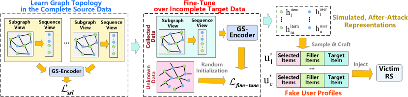
Figure 1: Overview of PC-Attack.

From Tab. 1, we can see that none of the existing methods have all the three properties illustrated in Sec. 1. In other words, there is still no real practical shilling attack method. Particularly, we do not find any method that has Property 2 and can achieve cross-system attack. Property 2 partially manifests in CopyAttack. But CopyAttack assumes the source data and the target data share items and it is only able to achieve cross-domain attack. Model Extraction Attack considers a data-free setting and uses limited queries ($c$ queries) to close the gap between the surrogate RS and the victim RS. But its idea only works on sequential RS and the number of required queries is hard to pre-defined.

In summary, based on Tab. 1, we can conclude that our method PC-Attack (illustrated in the next section) has all of the three properties that a practical shilling attack method should have. And it is able to achieve cross-system attack, a difficult but practical setting of real shilling attacks.

3 Our Framework PC-Attack

3.1 Motivation and Overview of PC-Attack

Existing works on cross-domain and cross-system recommendations (Zhao et al. 2013; Zhu et al. 2018) have verified that the knowledge learned from a source domain/system can help improve recommendation results in a target domain/system, i.e., the RS knowledge is transferable. This has inspired us in designing PC-Attack. We believe it is possible to have an attack model that captures RS knowledge from the source data and can be transferred to attack the victim RS. Fig. 1 provides an overview of PC-Attack:

1. Firstly, we construct a bipartite user-item graph on the source data where each user-item edge indicates the existence of the corresponding user-item interaction.

2. After that, PC-Attack trains a graph structure encoder (GS-Encoder) to capture the structural patterns of the source data in a self-supervised manner.

3. Then, PC-Attack feeds a small portion of the public target data (e.g., a popular item and some people who bought it) into GS-Encoder and fine-tunes to get simulated representations after a successful attack.

4. Finally, based on the simulated representations, PC-Attack searches for possible co-visit items of the target item that affect the possibility of recommending the target item and fills them in fake user profiles. Fake user profiles are injected into the victim RS to start the attack.

PC-Attack does not assume that the entity-correspondences across different domains/systems exist (i.e., a user or an item exists in both source and target data) even if they indeed exist. This way, PC-Attack does not require additional prior knowledge. Therefore, in step 2, PC-Attack is designed to only capture the structural patterns of the source data without knowing real identities of each node. To endow PC-Attack with the attack power, when constructing fake user profiles in step 4, we adopt the idea that items that can affect whether the target item is recommended are likely to have been interacted by some users together with the target item. This idea is called as co-visitation attack and has been verified in existing shilling attack methods (Yang, Gong, and Cai 2017). Compared to existing methods, PC-Attack requires much less information. It only needs a subgraph of a popular item, numbers of users/items in the target data and users who interacted with the target item before.

3.2 Learn from Graph Topology in the Source

Without the knowledge of explicit entity-correspondences between the source data and the target data, we can not directly leverage historical records in the source data to encode users and items into representations that can be later used in attacking the target data. Nevertheless, previous studies have shown that topologies of user-item bipartite graphs from different RS data share some common properties (Huang and Zeng 2011). We can construct a user-item bipartite graph from the source data and train a graph structure encoder (GS-Encoder) to capture graph topological properties that are shared among different RS domains/systems.

Graph Neural Network (GNN) is the prevalent neural network used for modeling graph data. We use GNN as the backbone of GS-Encoder to capture the intrinsic and transferable properties from interaction data in the bipartite graph. However, most feedback provided by users is implicit (e.g., clicks and views) rather than explicit (e.g., ratings). Hence, the observed interactions often contain noise that may not indicate real user preferences. Neighborhood aggregation schemes in GNN may amplify the influence of interactions on representation learning, making learning more susceptible to interaction noise.

To alleviate the negative effect of noise, we introduce contrastive learning, a type of self-supervised learning (SSL) (Liu et al. 2021), into GS-Encoder. SSL constructs supervision signals from the correlation within the input data, avoiding requiring implicit labels. Through contrasting samples, GS-Encoder learns to move similar sample pairs to stay close to each other while dissimilar ones are far apart. We adopt the idea of multi-view learning (Xu, Tao, and Xu 2013) when designing the self-supervised contrastive learning task. We model the node neighborhood as both a subgraph and a sequence, which helps GS-Encoder better capture the topological properties.

Multi-view Data Augmentation

To model node neighborhoods, we first sample paths by random walks and expand a single node $j$ in the user-item bipartite graph into its local structure as the subgraph view $g_{j}$. We use the random walk with a restart process (Tong, Faloutsos, and Pan 2006): (1) a random walk starts from a node $j$ in the bipartite graph, and (2) it randomly transmits to a neighbor with a probability $\alpha$ or returns to $j$ with a probability $1-\alpha$ in each step. Note that we re-construct subgraph views in each training epoch.

For each node, its 1-hop neighbors describe user-item interaction patterns. The 2-hop neighbors exhibit co-visitation patterns (i.e., users who have interacted with the same item or items which have been interacted by the same user), which are important in shilling attacks (Yang, Gong, and Cai 2017). We propose to construct the sequence view to capture the above two types of patterns better. With the node $j$ as the center, we sort by the ID of its 1-hop nodes and its 2-hop nodes in turn to construct the sequence view $s_{j}$ of $j$. The difference between the sequence view and the subgraph view is that the sequence view directly separates two data patterns while the subgraph view mixes two patterns up. Using the sequence view emphasizes learning two patterns individually while using the subgraph view learns them as a whole.

Multi-View Contrastive Learning

Contrastive learning aims to maximize the similarity between positive samples while minimizing the similarity between negative samples. A suitable contrast task will facilitate capturing topological properties from the source data. Unlike most contrastive learning methods that only focus on contrasting positive and negative samples in one view, we deploy a multi-view contrast mechanism when designing GS-Encoder so that GS-Encoder can benefit from more supervision signals.

The subgraph view of each node is passed to a GNN encoder in GS-Encoder. We adopt GIN (Xu et al. 2019) as the GNN encoder, though other GNNs can be adopted. The GNN encoder updates node representations as follows:

$$\mathbf{h}_{v}^{(b)}=\text{MLP}^{(b)}\big{(}(1+\epsilon^{(b)})\cdot\mathbf{h}_{v}^{(b-1)}+\Sigma_{u\in\mathcal{N}(v)}\mathbf{h}_{u}^{(b-1)}\big{)},$$ (1)

where $\mathbf{h}_{v}^{(b)}$ is the representation of node $v$ at the $b$-th GNN layer, $\mathcal{N}(v)$ is the set of 1-hop nodes to $v$ and $\text{MLP}(\cdot)$ indicates multi-layer perceptron. We use eigenvectors of the normalized graph Laplacian of the subgraph to initialize $\mathbf{h}^{(0)}$ of each node in the subgraph (Qiu et al. 2020). For a node $j$, its representation $\mathbf{h}_{j}^{g}$, from the subgraph view, is the concatenation of the aggregation of its neighborhood’s representations generated in all GNN layers:

$$\mathbf{h}_{j}^{g}=\text{Concat}\big{(}\text{Readout}(\{\mathbf{h}_{v}^{(b)}|v\in\mathcal{V}_{j}\})\,|\,b=0,1,...,\hat{b}\big{)},$$ (2)

where $\text{Concat}(\cdot)$ denotes the concatenate operation, the $\text{Readout}(\cdot)$ function aggregates representations of nodes in the subgraph of $j$ from each iteration, and $\hat{b}$ is the number of GIN layers.

The sequence view of each node $j$ is passed to a LSTM and we use the last hidden state $\mathbf{h}^{s}_{j}$ as the representation from the sequence view.

$\mathbf{h}^{g}$ and $\mathbf{h}^{s}$ are further fed to a fully connected feedforward neural network to map them to the same latent space:

$$\hat{\mathbf{h}}_{j}^{g}=\textbf{W}_{2}\cdot\sigma(\textbf{W}_{1}\mathbf{h}_{j}^{g}+\textbf{b}_{1})+\textbf{b}_{2},$$ (3)

$$\hat{\mathbf{h}}_{j}^{s}=\textbf{W}_{2}\cdot\sigma(\textbf{W}_{1}\mathbf{h}_{j}^{s}+\textbf{b}_{1})+\textbf{b}_{2},$$

where $\textbf{W}_{1},\textbf{W}_{2},\textbf{b}_{1},\textbf{b}_{2}$ are learnable weights, and $\sigma(\cdot)$ indicates the sigmoid function.

In contrastive learning, we need to define positive and negative samples. For each node $j$, we define its positive sample $\mathit{pos}_{j}$ and negative samples $\mathit{neg}_{j}$ as the subgraph obtained by random walks starting from $j$ and its corresponding sequence view, and the subgraphs obtained by random walks starting from other nodes and their corresponding sequence views, respectively. Note that, to improve efficiency and avoid processing too many negative subgraphs/sequences, we use subgraph/sequence views of other nodes in the same batch as negative samples.

The contrastive loss under the subgraph view is:

$$\mathcal{L}_{j}^{g}=-log\frac{exp\big{(}sim(\hat{\mathbf{h}}_{j}^{g},\hat{\mathbf{h}}_{\mathit{pos}_{j}}^{s})/\tau\big{)}}{\Sigma_{l\in\mathit{neg}_{j}}exp\big{(}sim(\hat{\mathbf{h}}_{j}^{g},\hat{\mathbf{h}}_{l}^{s})/\tau\big{)}},$$ (4)

where $\text{sim}(\cdot)$ denotes the cosine similarity and $\tau$ denotes a temperature parameter. The contrastive loss under the sequence view is defined similarly:

$$\mathcal{L}_{j}^{s}=-log\frac{exp\big{(}sim(\hat{\mathbf{h}}_{j}^{s},\hat{\mathbf{h}}_{\mathit{pos}_{j}}^{g})/\tau\big{)}}{\Sigma_{l\in\mathit{neg}_{j}}exp\big{(}sim(\hat{\mathbf{h}}_{j}^{s},\hat{\mathbf{h}}_{l}^{g})/\tau\big{)}}.$$ (5)

The overall multi-view contrastive objective of GS-Encoder is as follows:

$$\mathcal{L}_{ssl}=\frac{1}{n}\Sigma_{j\in\mathcal{I}}(\lambda_{g}\cdot\mathcal{L}_{j}^{g}+\lambda_{s}\cdot\mathcal{L}_{j}^{s}),$$ (6)

where $\lambda_{g}$ and $\lambda_{s}$ are hyper-parameters to balance two views, $\mathcal{I}$ is the item set, and $n$ is the number of items.

3.3 Craft Fake User Profiles in the Victim RS

After pre-training the GS-Encoder, the next step is to construct a few fake user profiles and inject them into the victim RS to pollute the target data. Our construction method of fake users is based on three design principles from the literature:

• Principle 1: Item-based RS is designed to recommend items similar to past items in the target user’s profile (Sarwar et al. 2001).

• Principle 2: User-based RS is designed to recommend items interacted by similar users of the target user (Herlocker, Konstan, and Riedl 2000).

• Principle 3: According to the idea of co-visitation attack (Yang, Gong, and Cai 2017), the co-visit items of the target item (i.e., the 2-hop neighbors of the target item in the bipartite graph) can affect whether the target item can be recommended.

Based on the above principles, the goals of our construction method are:

• Goal 1: Based on Principle 1, our goal is to affect the victim RS so that the representation of target item is as similar as possible to representations of the rest of the items. This way, the possibility of recommending the target item can increase. We hope that our attack can achieve the following objective: for any item $i$, $sim(\mathbf{h}^{item}_{i},\mathbf{h}^{item}_{t})>sim(\mathbf{h}^{item}_{i},\mathbf{h}^{item}_{j})$, where $t$ is the target item, $j$ denotes any other item, and $sim(\cdot)$ denotes a measure of similarity between items (e.g., cosine similarity), and $\mathbf{h}^{item}_{i}$ is the representation of item $i$ in the victim RS.

• Goal 2: Based on Principle 2, our goal is to affect the victim RS so that representations of users who have interacted with the target item are as similar as possible to representations of other users. This way, the possibility of recommending the target item can increase. We hope that, for any user $u$, $sim(\mathbf{h}^{user}_{u},\mathbf{h}^{user}_{r})>sim(\mathbf{h}^{user}_{u},\mathbf{h}^{user}_{e})$, where $r\in\mathcal{N}(t)$ denotes the user who has interacted with the target item $t$, $e\notin\mathcal{N}(t)$ is any other user, and $\mathbf{h}^{user}_{u}$ is the representation of user $u$ in the victim RS.

• Goal 3: Based on Principle 3, our goal is to find possible co-visit items of the target item after a successful attack and fill them in the fake user profiles.

However, the above goals are challenging without knowing the details of the victim RS and the target data, i.e., we do not know $\mathbf{h}^{item}$ and $\mathbf{h}^{user}$ in the victim RS. GS-Encoder, which captures the transferable knowledge from the more informative source data, can help us accomplish this task:

• Step 1: Use the pre-trained GS-Encoder to generate node representations based on topological information of the incomplete target data.

• Step 2: Fine-tune and get simulated representations after the successful attack (Goal 1 and Goal 2).

• Step 3: Based on the simulated, after-attack representations, we search for possible co-visit items of the target items and craft the fake user profiles (Goal 3).

Considering that we cannot access the complete target data, we collect a very small portion of the target data that can be publicly accessed. One example is the popular item in the victim RS, some normal users who have bought them and the 2-hop items to the popular item. Such information is typically available. For instance, Amazon provides “Popular Items This Season” and Newsegg provides “Popular Products” on their homepages, as shown in Fig. 2, and information of their buyers can be found by clicking the popular item. The buyer’s homepage may provide information of some items that he/she bought before. Therefore, starting from one popular item, we collect users/items in its 2-hop subgraph via random walks without restart. But we limit the total number of nodes to be lower than $p$ percentage of the target data to keep a low level of knowledge. In addition to the collected subgraph of a popular item, we collect a user set $\mathcal{M}(t)$ containing users who have interacted with the target item $t$.

Figure 2: Popular items of Amazon and Newegg.

Based on the collected data from the target data, we construct a small subgraph centering on the popular item, and feed it into the pre-trained GS-Encoder to generate initial representations of users/items in the subgraph:

$$\mathbf{h}_{j}=\eta_{g}\cdot\hat{\mathbf{h}}_{j}^{g}+\eta_{s}\cdot\hat{\mathbf{h}}_{j}^{s},$$ (7)

where $\eta_{g}$ and $\eta_{s}$ are hyper-parameters that balance the effects of the two views, $\mathbf{h}_{j}$ is the fused representation of node $j$, and $\hat{\mathbf{h}}_{j}^{g}$ and $\hat{\mathbf{h}}_{j}^{s}$ are subgraph-view representation and sequence-view representation of node $j$ generated by the pre-trained GS-Encoder as shown in Eq. 3, respectively.

For most users and items in the target data that are not collected, we assume that we know the numbers of users ($m$) and items ($n$) in the victim RS, and initialize their representations from a normal distribution $\mathcal{N}(0,0.1)$. This is a reasonable assumption as many RS websites reveal exact numbers or the order of magnitude of users/items. Including users and items that are not in the collected small subgraph makes it possible to generate fake user profiles with items not in the collected subgraph.

We continue to fine-tune over the above collected data with the following objective for Goal 1 to simulate representations after a successful attack:

$$\mathcal{L}^{item}=-log\Sigma_{i=1}^{n}\frac{sim(\mathbf{h}_{i}^{item},\mathbf{h}_{t}^{item})}{\Sigma_{j\neq t}sim(\mathbf{h}_{i}^{item},\mathbf{h}_{j}^{item})}.$$ (8)

Similarly, for Goal 2, we fine-tune with the following objective to simulate representations after a successful attack:

$$\mathcal{L}^{user}=-log\Sigma_{u=1}^{m}\frac{\Sigma_{g\in\mathcal{M}(t)}sim(\mathbf{h}^{user}_{u},\mathbf{h}^{user}_{g})}{\Sigma_{j\notin\mathcal{M}(t)}sim(\mathbf{h}^{user}_{u},\mathbf{h}^{user}_{j})}.$$ (9)

The overall objective is as follows:

$$\mathcal{L}_{fine-tune}=\mu_{item}\cdot\mathcal{L}^{item}+\mu_{user}\cdot\mathcal{L}^{user},$$ (10)

where $\mu_{item}$ and $\mu_{user}$ are hyper-parameters that balance the effects of the two loss functions.

After fine-tuning, we have new representations of users and items that simulate the representations in the victim RS after a successful attack. Then, we search for possible co-visit items of the target item based on the simulated representations. Similar to other shilling attack methods (Lin et al. 2020, 2022), the fake user profile in PC-Attack contains three parts: selected items, filler items and the target item. We estimate the potential interest of all users in the target item $t$ after the attack by the inner product of representations, and sample $z$ users according to the probability:

$$Pro(u|t)=\frac{\mathbf{h}^{item}_{t}\cdot\mathbf{h}^{user}_{u}}{\Sigma_{j=1}^{m}\mathbf{h}^{item}_{t}\cdot\mathbf{h}^{user}_{j}}.$$ (11)

Common items existing in these $z$ profiles are chosen as the selected items. Because popular items are always more accessible than others and appear in many normal users’ profiles, we randomly sample $y$ popular items from the collected subgraph according to their degrees as filler items to enhance the invisibility of PC-Attack. For each fake profile, the above crafting process is conducted independently.

4 Experiments

Dataset	#Users	#Items	#Interactions	Sparsity
FilmTrust	780	721	28,799	94.88%
Automotive	2,928	1,835	20,473	99.62%
T & HI	1,208	8,491	28,396	99.72%
Yelp	2,762	10,477	119,237	99.59%

Table 2: Statistics of datasets

Dataset	Victim RS	Attack Method (HR@50)
		RevAdv	TrialAttack	Leg-UP	AUSH	Bandwagon	Random	Segment	PC-Attack∗	PC-Attack
Automotive	CDAE	0.1643	0.2504	0.2237	0.1949	0.2114	0.2247	0.1949	0.1348	0.1693
	ItemAE	0.2916	0.3128	0.3105	0.2926	0.3232	0.3183	0.2926	0.4908	0.3787
	LightGCN	0.1002	0.1228	0.1149	0.1361	0.1462	0.1222	0.1361	0.1406	0.1716
	NCF	0.7012	0.7744	0.7712	0.7359	0.7689	0.7462	0.7359	0.8574	0.6484
	NGCF	0.0866	0.0960	0.1398	0.1416	0.1362	0.1387	0.1416	0.0864	0.1056
	VAE	0.0842	0.0841	0.1168	0.1196	0.0960	0.0965	0.1196	0.1238	0.1559
	WRMF	0.9243	0.2941	0.3561	0.4386	0.3769	0.3069	0.4386	0.9268	0.9213
FilmTrust	CDAE	0.4587	0.6270	0.6190	0.5342	0.4837	0.5954	0.5342	0.7505	0.7810
	ItemAE	0.6429	0.4721	0.5965	0.5501	0.5253	0.4807	0.5501	0.9534	0.9544
	LightGCN	0.8522	0.8362	0.8820	0.8594	0.8271	0.8169	0.8594	0.8949	0.8517
	NCF	0.9319	0.9108	0.9521	0.8846	0.8855	0.8929	0.8846	0.9266	0.9543
	NGCF	0.9015	0.9123	0.9207	0.9072	0.9079	0.9091	0.9072	0.9037	0.9101
	VAE	0.9713	0.9742	0.9749	0.9724	0.9721	0.9726	0.9724	0.9689	0.9730
	WRMF	0.5143	0.4171	0.4732	0.4976	0.4873	0.4667	0.4976	0.5706	0.4935
T & HI	CDAE	0.1126	0.3186	0.3929	0.3409	0.3173	0.4156	0.3409	0.3449	0.2279
	ItemAE	0.1074	0.2755	0.2677	0.1433	0.1857	0.2335	0.1433	0.3324	0.1487
	LightGCN	0.0028	0.0376	0.0383	0.0531	0.1603	0.0273	0.0531	0.0456	0.2064
	NCF	0.5421	0.6895	0.8508	0.8038	0.9017	0.8827	0.8038	0.7749	0.1988
	NGCF	0.0177	0.0739	0.1018	0.0903	0.1016	0.0927	0.0903	0.1064	0.0705
	VAE	0.3530	0.9975	0.9993	0.9995	0.9991	0.9996	0.9995	0.9916	0.9669
	WRMF	0.0406	0.0697	0.0495	0.0448	0.0530	0.0460	0.0448	0.0868	0.0743

Table 3: Attack performance (HR@50) of different attack methods against different victim RS models. PC-Attack^∗ indicates that the complete target data is used. Best results are shown in bold.

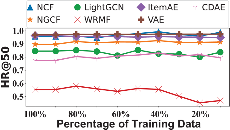
Figure 3: Impacts of Accessible Target Data ($p$).

Victim RS	Source Data
	Automotive		T & HI		Yelp
	HR@50	NDCG@50	HR@50	NDCG@50	HR@50	NDCG@50
CDAE	0.773	0.198	0.793	0.199	0.781	0.200
ItemAE	0.953	0.257	0.949	0.255	0.954	0.257
LightGCN	0.817	0.219	0.823	0.221	0.852	0.236
NCF	0.907	0.247	0.927	0.254	0.954	0.256
NGCF	0.895	0.243	0.909	0.242	0.910	0.247
VAE	0.971	0.259	0.970	0.258	0.973	0.259
WRMF	0.508	0.139	0.475	0.131	0.494	0.136

Table 4: Results of using different source datasets (the target dataset is FilmTrust). Best results are shown in bold.

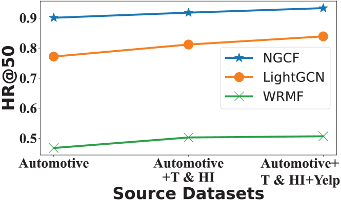
Figure 4: Learn graph topology from multiple source datasets and then attack victim RS on FilmTrust.

Victim RS	Target Data
	FilmTrust		Automotive		T & HI
	Precison	Recall	Precison	Recall	Precison	Recall
RevAdv	0.0713	0.0778	0.0080	0.0089	0.0180	0.0200
TrialAttack	0.1603	0.1927	0.1114	0.1038	0.0200	0.0256
Leg-UP	0.2497	0.2711	0.0000	0.0000	0.0400	0.0444
AUSH	0.2429	0.2556	0.0380	0.0422	0.0742	0.0822
Bandwagon	0.2371	0.2489	0.0220	0.0244	0.0762	0.0845
Random	0.2340	0.2467	0.0220	0.0244	0.0441	0.0489
Segment	0.2602	0.2733	0.0280	0.0311	0.0662	0.0733
PC-Attack	0.0280	0.0311	0.0000	0.0000	0.0240	0.0266

Table 5: Detection performance on different attack methods. Best results are shown in bold.

4.1 Experimental Settings

Datasets

We use four public datasets widely adopted in previous works on shilling attacks (Lin et al. 2020, 2022), including FilmTrust, Yelp and two other Amazon datasets Automotive, and Tools & Home Improvement (T & HI). Target items for testing attacks are included in the datasets. Tab. 2 illustrates the statistics of the data. Default training/test split is used for training and tuning surrogate RS models (if baselines require a surrogate RS) and victim RS models. By default, we train PC-Attack to learn graph topology from the complete Yelp dataset since Yelp is the largest dataset. Then, we test it on attacking victim RS on the other three datasets. Since some experiments require long-tail items, we define long-tail items as items with no more than three interactions.

Shilling Attack Baselines

We use three classic attack methods² Random Attack, Bandwagon Attack and Segment Attack (Lin et al. 2022), and four state-of-the-art shilling attack methods RevAdv (Tang, Wen, and Wang 2020), TrialAttack (Wu et al. 2021), Leg-UP² (Lin et al. 2022) and AUSH² (Lin et al. 2020) as baselines.

Victim RS

We conduct shilling attacks against various prevalent RS models: NCF (He et al. 2017), WRMF (Hu, Koren, and Volinsky 2008), LightGCN (He et al. 2020), NGCF (Wang et al. 2019), VAE (Liang et al. 2018), CDAE (Wu et al. 2016) and ItemAE (Sedhain et al. 2015).

Hyper-parameters

The hyper-parameters of attack baselines and victim RS are set as the original papers suggest and tuned to show the best results. We set the number of fake profiles to 50 for all methods. This is roughly the population that can manifest the differences among attack models (Burke et al. 2005). For PC-Attack, we set training epochs to 32, batch size to 32, embedding size to 64 and learning rate to 0.005. $z$ and $y$ used in crafting profiles are set to 50 and 10, respectively. The length of random walk is set to 64 and the restart probability $1-\alpha$ is 0.8. The number of GIN layers $\hat{b}$ is 5. Other hyper-parameters of PC-Attack are selected through grid search and the chosen hyper-parameters are: $\tau=0.07$, $\lambda_{g}=0.5$, $\lambda_{s}=0.5$, $\eta_{g}=0.5$, $\eta_{s}=0.5$, $\mu_{user}=0.5$, and $\mu_{item}=0.5$. By default, we set $p=10\%$ when collecting target data. Adam optimizer is adopted for optimization.

Evaluation Metrics

Hit Ratio (HR@k) and Normalized Discounted Cumulative Gain (NDCG@k) are used for evaluation. HR@k measures the average proportion of normal users whose top-k recommendation lists contain the target item after the attack. NDCG@k measures the ranking of the target item after the attack. For both metrics, we set k to 50.

4.2 Overall Attack Performance

Tab. 3 summarizes the overall attack performance of different attack methods. We have the following observations:

1. PC-Attack^∗ and PC-Attack together achieve the best results in most cases, showing the effectiveness of our designs. Some baselines may have better results in a few cases, but their attack performance is not robust.

2. PC-Attack achieves best results in more than 30% cases. In other cases where PC-Attack does not rank first, its performance is not far away from the best performance. Note that our goal (i.e., a practical attack) is to use as little information of the target data as possible. In the case of the unfair comparison, (i.e., baselines take the complete target data and PC-Attack accesses at most 10%), it is acceptable that PC-Attack can have degraded performance in exchange for the feasibility of the attack. However, PC-Attack shows promising results, showing the power of cross-system attack.

4.3 Impacts of Accessible Target Data ($p$)

We evaluate the performance of PC-Attack when $p$ changes (the default value is $p=10\%$ and PC-Attack^∗ uses $p=100\%$). Fig. 3 illustrates the results on the FilmTrust dataset. We can observe that, as $p$ decreases, the attack performance of PC-Attack degrades gradually. However, thanks to the knowledge learned from the source data, the decline of attack performance is not significant and PC-Attack is robust when the percentage of accessible target data varies.

4.4 Impacts of Source Data

We conduct two experiments to check the impacts of source data on PC-Attack:

Impacts of Using Different Source Data

Tab. 4 reports the results of PC-Attack when using FilmTrust as the target data and the other three datasets are used as the source data. We can observe that using different source dataset does not affect the performance too much, which confirms that different RS data have common topological information of which the knowledge is transferable. However, the larger the source data is, the better PC-Attack can capture the structural patterns. Hence, PC-Attack shows best results when using Yelp (the largest dataset in our experiments) as the source data.

Performance of Using Multiple Source Datasets

PC-Attack can learn graph topology from multiple source datasets to benefit from the large volume of public RS data. To illustrate the results of using multiple source dataset, we train PC-Attack on different source datasets in the order of dataset size and then use it to attack WRMF, NGCF and LightGCN on the FilmTrust dataset. As shown in Fig. 4, as more source datasets are used, the performance of PC-Attack gradually gets improved, showing that we can feed more public RS datasets to PC-Attack and get even better attack performance.

4.5 Attack Invisibility

Next, we investigate the invisibility of PC-Attack.

Attach Detection

We apply the state-of-the-art unsupervised attack detector (Zhang et al. 2015) on the fake profiles generated by different attack methods. Tab. 5 describes the accuracy and recall of the detector on different attack methods. Lower precision and recall indicate that the attack method is less perceptible. Based on the results, we find that the detection performance is highly data-dependent, and fake users are more easy to detect on denser datasets. For example, it is difficult for the detector to find fake users on Yelp. But it has relatively high precision and recall for detecting most attack methods (except PC-Attack) on FilmTrust. PC-Attack generates almost undetectable fake users. In most cases, the detector performs the worst on PC-Attack. On T & HI, the detector does not has the lowest precision and recall for PC-Attack, but the values are close to lowest ones.

Fake User Distribution

Using t-SNE (Van der Maaten and Hinton 2008), Fig. 5 visualizes users’ representations generated by WRMF after it is attacked by PC-Attack on Automotive and FilmTrust. We can observe that fake users profiles are scattered among real user profiles and it is hard for detectors to distinguish fake and real users, showing that PC-Attack can launch virtually invisible attacks.

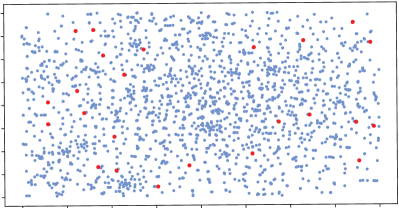
(a) Automotive

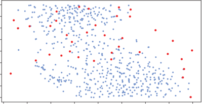
(b) FilmTrust

Figure 5: Visualization of user profiles. Red nodes are fake profiles and blue nodes are real profiles.

4.6 Impacts of the Starting Node in Target Data

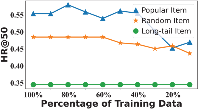
Figure 6: Impact of the starting item.

By default, we start with the most popular item to collect the target data and select no more than 10% of user-item interaction records within the limit of only 2-hop neighbors. To evaluate the robustness of PC-Attack, we compare the default setting with two other options: use an item sampled from long-tail items as the starting point and use a random sampled item as the starting point. Fig. 6 compares the results of the default setting and two extra settings for attacking WRMF on FilmTrust. We can see that the attack performance of starting with a randomly sampled item does not lag much behind starting with the most popular item, and is also robust w.r.t. different settings of total numbers of nodes in the collected target data. Differently, starting from a sampled long-tail item results in a much worse performance. The reason is the long-tail item does not have many 2-hop neighbors and the collected data cannot help fine-tune GS-Encoder well on the target data. The performance of starting from a long-tail item is very consistent when the limit of node numbers changes. The reason is that long tail items have few neighbors and the number of the 2-hop neighbors of long tail items do not exceed 10% of the total target data. Changing the limit does not actually change the number of the collected nodes. In summary, starting with a popular item brings the best results. Considering that popular items are always more readily available, PC-Attack uses the popular item as the default starting point to collect target data.

4.7 Performance of Cross-domain Attack.

Victim RS	T & HI $\rightarrow$ Automotive		Automotive $\rightarrow$ T & HI
	HR@50	NDCG@50	HR@50	NDCG@50
CDAE	0.035	0.008	0.222	0.068
ItemAE	0.288	0.096	0.142	0.080
LightGCN	0.160	0.051	0.238	0.113
NCF	0.366	0.084	0.079	0.036
NGCF	0.039	0.009	0.061	0.018
VAE	0.047	0.011	0.975	0.565
WRMF	0.902	0.288	0.073	0.027

Table 6: Results of PC-Attack for the cross-domain attack.

$\eta_{g}:\eta_{s}$	HR@50	NDCG@50	$\lambda_{g}:\lambda_{s}$	HR@50	NDCG@50	$\mu_{item}:\mu_{user}$	HR@50	NDCG@50
1:0	0.467	0.131	1:0	0.471	0.132	1:0	0.474	0.131
0:1	0.471	0.132	0:1	0.478	0.134	0:1	0.477	0.114
2:1	0.499	0.134	2:1	0.515	0.147	2:1	0.481	0.136
1:2	0.486	0.136	1:2	0.512	0.144	1:2	0.501	0.142
1:1	0.522	0.146	1:1	0.522	0.146	1:1	0.522	0.146

Table 7: Results using different hyper-parameters.

PC-Attack is designed for both cross-system attack and cross-domain attack. Experimental results in previous sections are for cross-system attack. Next, we further report the performance of cross-domain attack using PC-Attack. Tab. 6 provides the result of PC-Attack for using T & HI as the source and Automotive as the target, and using Automotive as the source and T & HI as the target. The two datasets contain data in different categories of Amazon. From the result, we can observe that PC-Attack achieves acceptable attack performance for cross-domain attack, but the performance is worse than cross-system attack reported in Tab. 3. The reason is that the source dataset Yelp used in our default experiments for cross-system attack is much larger than T & HI and Automotive used in the experiments for cross-domain attack. PC-Attack can better capture topological information from a larger source dataset. Hence, it shows better results in cross-system attack than cross-domain attack.

4.8 Impacts of Hyper-parameters and Ablation Study

The three sets of balance hyper-parameters $\eta$, $\lambda$ and $\mu$ are used to balance the effects of representations from graph and sequence views, graph-view and sequence-view loss functions, and user and item loss functions, respectively.

Tab. 7 reports the performance of PC-Attack when attacking WRMF using different balance hyper-parameters. We can observe that the change of balance hyper-parameters affect the performance of PC-Attack. When setting equal values to all balance hyper-parameters, the attack performance is the best.

Besides, the first two rows and the last row in Tab. 7 can be viewed as three ablation experiments: (1) only use graph-view representation, graph-view loss and item loss, (2) only use sequence-view representation, sequence-view loss and sequence loss, and (3) the default PC-Attack that uses all parts. From Tab. 7, we can see that PC-Attack performs best when all parts are present and removing any of them will degrade the attack performance. Therefore, we can conclude that each component in PC-Attack indeed contributes to its overall attack performance.

5 Conclusion

In this paper, we study practical shilling attacks. We analyze the limitations of existing works and design a new framework PC-Attack that transfers the knowledge to attack the victim RS on incomplete target dataset. Experimental results demonstrate the superiority of PC-Attack. In the future, we plan to introduce more self-supervised learning tasks so that PC-Attack can get more supervision signals and better capture the transferable RS knowledge.

References

- Burke et al. (2005) Burke, R. D.; Mobasher, B.; Bhaumik, R.; and Williams, C. 2005. Segment-Based Injection Attacks against Collaborative Filtering Recommender Systems. In ICDM, 577–580.
- Christakopoulou and Banerjee (2019) Christakopoulou, K.; and Banerjee, A. 2019. Adversarial attacks on an oblivious recommender. In RecSys, 322–330.
- Deldjoo, Noia, and Merra (2021) Deldjoo, Y.; Noia, T. D.; and Merra, F. A. 2021. A Survey on Adversarial Recommender Systems: From Attack/Defense Strategies to Generative Adversarial Networks. ACM Comput. Surv., 54(2): 35:1–35:38.
- Fan et al. (2021) Fan, W.; Derr, T.; Zhao, X.; Ma, Y.; Liu, H.; Wang, J.; Tang, J.; and Li, Q. 2021. Attacking Black-box Recommendations via Copying Cross-domain User Profiles. In ICDE, 1583–1594.
- Goodfellow et al. (2014) Goodfellow, I. J.; Pouget-Abadie, J.; Mirza, M.; Xu, B.; Warde-Farley, D.; Ozair, S.; Courville, A. C.; and Bengio, Y. 2014. Generative Adversarial Nets. In NIPS, 2672–2680.
- Gou et al. (2021) Gou, J.; Yu, B.; Maybank, S. J.; and Tao, D. 2021. Knowledge Distillation: A Survey. Int. J. Comput. Vis., 129(6): 1789–1819.
- Gunes et al. (2014) Gunes, I.; Kaleli, C.; Bilge, A.; and Polat, H. 2014. Shilling attacks against recommender systems: a comprehensive survey. Artif. Intell. Rev., 42(4): 767–799.
- He et al. (2020) He, X.; Deng, K.; Wang, X.; Li, Y.; Zhang, Y.; and Wang, M. 2020. LightGCN: Simplifying and Powering Graph Convolution Network for Recommendation. In SIGIR, 639–648.
- He et al. (2017) He, X.; Liao, L.; Zhang, H.; Nie, L.; Hu, X.; and Chua, T. 2017. Neural Collaborative Filtering. In WWW, 173–182.
- Herlocker, Konstan, and Riedl (2000) Herlocker, J. L.; Konstan, J. A.; and Riedl, J. 2000. Explaining collaborative filtering recommendations. In CSCW, 241–250.
- Hu, Koren, and Volinsky (2008) Hu, Y.; Koren, Y.; and Volinsky, C. 2008. Collaborative Filtering for Implicit Feedback Datasets. In ICDM, 263–272.
- Huang and Zeng (2011) Huang, Z.; and Zeng, D. D. 2011. Why Does Collaborative Filtering Work? Transaction-Based Recommendation Model Validation and Selection by Analyzing Bipartite Random Graphs. INFORMS J. Comput., 23(1): 138–152.
- Kaelbling, Littman, and Moore (1996) Kaelbling, L. P.; Littman, M. L.; and Moore, A. W. 1996. Reinforcement Learning: A Survey. J. Artif. Intell. Res., 4: 237–285.
- Lam and Riedl (2004) Lam, S. K.; and Riedl, J. 2004. Shilling recommender systems for fun and profit. In WWW, 393–402.
- Li et al. (2016) Li, B.; Wang, Y.; Singh, A.; and Vorobeychik, Y. 2016. Data Poisoning Attacks on Factorization-Based Collaborative Filtering. In NIPS, 1885–1893.
- Liang et al. (2018) Liang, D.; Krishnan, R. G.; Hoffman, M. D.; and Jebara, T. 2018. Variational Autoencoders for Collaborative Filtering. In WWW, 689–698.
- Lin et al. (2020) Lin, C.; Chen, S.; Li, H.; Xiao, Y.; Li, L.; and Yang, Q. 2020. Attacking Recommender Systems with Augmented User Profiles. In CIKM, 855–864.
- Lin et al. (2022) Lin, C.; Chen, S.; Zeng, M.; Zhang, S.; Gao, M.; and Li, H. 2022. Shilling Black-box Recommender Systems by Learning to Generate Fake User Profiles. IEEE Trans. Neural Networks Learn. Syst.
- Liu et al. (2021) Liu, X.; Zhang, F.; Hou, Z.; Mian, L.; Wang, Z.; Zhang, J.; and Tang, J. 2021. Self-supervised Learning: Generative or Contrastive. IEEE Trans. Knowl. Data Eng.
- Qiu et al. (2020) Qiu, J.; Chen, Q.; Dong, Y.; Zhang, J.; Yang, H.; Ding, M.; Wang, K.; and Tang, J. 2020. GCC: Graph Contrastive Coding for Graph Neural Network Pre-Training. In KDD, 1150–1160.
- Sarwar et al. (2001) Sarwar, B. M.; Karypis, G.; Konstan, J. A.; and Riedl, J. 2001. Item-based collaborative filtering recommendation algorithms. In WWW, 285–295.
- Sedhain et al. (2015) Sedhain, S.; Menon, A. K.; Sanner, S.; and Xie, L. 2015. AutoRec: Autoencoders Meet Collaborative Filtering. In WWW (Companion Volume), 111–112.
- Song et al. (2020) Song, J.; Li, Z.; Hu, Z.; Wu, Y.; Li, Z.; Li, J.; and Gao, J. 2020. PoisonRec: An Adaptive Data Poisoning Framework for Attacking Black-box Recommender Systems. In ICDE, 157–168.
- Tang, Wen, and Wang (2020) Tang, J.; Wen, H.; and Wang, K. 2020. Revisiting Adversarially Learned Injection Attacks Against Recommender Systems. In RecSys, 318–327.
- Tong, Faloutsos, and Pan (2006) Tong, H.; Faloutsos, C.; and Pan, J. 2006. Fast Random Walk with Restart and Its Applications. In ICDM, 613–622.
- Van der Maaten and Hinton (2008) Van der Maaten, L.; and Hinton, G. 2008. Visualizing data using t-SNE. Journal of machine learning research, 9(11).
- Wang et al. (2019) Wang, X.; He, X.; Wang, M.; Feng, F.; and Chua, T. 2019. Neural Graph Collaborative Filtering. In SIGIR, 165–174.
- Wu et al. (2021) Wu, C.; Lian, D.; Ge, Y.; Zhu, Z.; and Chen, E. 2021. Triple Adversarial Learning for Influence based Poisoning Attack in Recommender Systems. In KDD, 1830–1840.
- Wu et al. (2016) Wu, Y.; DuBois, C.; Zheng, A. X.; and Ester, M. 2016. Collaborative Denoising Auto-Encoders for Top-N Recommender Systems. In WSDM, 153–162.
- Xing et al. (2013) Xing, X.; Meng, W.; Doozan, D.; Snoeren, A. C.; Feamster, N.; and Lee, W. 2013. Take This Personally: Pollution Attacks on Personalized Services. In USENIX Security Symposium, 671–686.
- Xu, Tao, and Xu (2013) Xu, C.; Tao, D.; and Xu, C. 2013. A Survey on Multi-view Learning. arXiv Preprint. https://arxiv.org/abs/1304.5634.
- Xu et al. (2019) Xu, K.; Hu, W.; Leskovec, J.; and Jegelka, S. 2019. How Powerful are Graph Neural Networks? In ICLR.
- Yang, Gong, and Cai (2017) Yang, G.; Gong, N. Z.; and Cai, Y. 2017. Fake Co-visitation Injection Attacks to Recommender Systems. In NDSS.
- Yuan et al. (2019) Yuan, X.; He, P.; Zhu, Q.; and Li, X. 2019. Adversarial Examples: Attacks and Defenses for Deep Learning. IEEE Trans. Neural Networks Learn. Syst., 30(9): 2805–2824.
- Yue et al. (2021) Yue, Z.; He, Z.; Zeng, H.; and McAuley, J. J. 2021. Black-Box Attacks on Sequential Recommenders via Data-Free Model Extraction. In RecSys, 44–54.
- Zhang et al. (2020) Zhang, H.; Li, Y.; Ding, B.; and Gao, J. 2020. Practical Data Poisoning Attack against Next-Item Recommendation. In WWW, 2458–2464.
- Zhang et al. (2021a) Zhang, H.; Tian, C.; Li, Y.; Su, L.; Yang, N.; Zhao, W. X.; and Gao, J. 2021a. Data Poisoning Attack against Recommender System Using Incomplete and Perturbed Data. In KDD, 2154–2164.
- Zhang et al. (2021b) Zhang, X.; Chen, J.; Zhang, R.; Wang, C.; and Liu, L. 2021b. Attacking Recommender Systems With Plausible Profile. IEEE Trans. Inf. Forensics Secur., 16: 4788–4800.
- Zhang et al. (2015) Zhang, Y.; Tan, Y.; Zhang, M.; Liu, Y.; Chua, T.; and Ma, S. 2015. Catch the Black Sheep: Unified Framework for Shilling Attack Detection Based on Fraudulent Action Propagation. In IJCAI, 2408–2414.
- Zhao et al. (2013) Zhao, L.; Pan, S. J.; Xiang, E. W.; Zhong, E.; Lu, Z.; and Yang, Q. 2013. Active Transfer Learning for Cross-System Recommendation. In AAAI.
- Zhu et al. (2018) Zhu, F.; Wang, Y.; Chen, C.; Liu, G.; Orgun, M. A.; and Wu, J. 2018. A Deep Framework for Cross-Domain and Cross-System Recommendations. In IJCAI, 3711–3717.