Event-based Backpropagation for Analog Neuromorphic Hardware

Event-based Backpropagation for Analog Neuromorphic Hardware

Abstract

Brain-inspired or neuromorphic computing aims to incorporate lessons from studying biological-nervous systems in the design of practical computer architectures. While existing approaches have successfully implemented aspects of those computational principles, such as sparse spike-based computation, event-based scalable learning has remained an elusive goal in large-scale systems. Reaching this goal is important because only then the potential energy-efficiency advantages of neuromorphic systems relative to other hardware architectures can be realized during learning. We present our progress implementing such an event-based algorithm for learning —the EventProp Algorithm— using the example of the BrainScaleS-2 analog neuromorphic hardware. Previous gradient-based approaches to learning used “surrogate gradients” and dense sampling of system observables or were limited by assumptions on the underlying dynamics and loss functions. In contrast, our approach does only need spike time observations from the system while being able to incorporate other system observables, such as membrane voltage measurements, in a principled way. This leads to a one-order-of-magnitude improvement in the information efficiency of the gradient estimate, which would directly translate to corresponding energy efficiency improvements in an optimized hardware implementation. We present the theoretical framework for estimating gradients and results verifying the correctness of the gradient estimation, as well as experimental results on a low-dimensional classification task using the BrainScaleS-2 system. Building on this work has the potential to enable scalable gradient estimation in large-scale neuromorphic hardware, including those using novel nano-devices, as a continuous measurement of the system state would be prohibitive and energy-inefficient in such instances. It also suggests the feasibility of a full on-device implementation of the algorithm that would enable scalable, energy-efficient, event-based learning in large-scale analog neuromorphic hardware.

[acronym]long-short acronym1

Neuromorphic or brain-inspired hardware aims to incorporate lessons and metaphors derived from biological nervous systems into the design of practical computer architectures. Many complementary approaches exist, ranging from digital implementations to architectures involving novel nano-devices. They have in common that they conceptualize computation as occurring in a network of processing elements —“neurons” exchanging messages “spikes”— with varying amounts of flexibility in the realizable network topology and configurability of the processing elements. The question then becomes how to endow such a network with function. While there are, in principle, many approaches, some taking inspiration from local learning rules postulated in computational neuroscience a by now well-established approach is to use machine-learning techniques and, in particular, gradient-based optimization methods.

In-the-loop gradient-based training on digital neuromorphic hardware was demonstrated on the TrueNorth system (Merolla et al., 2014; Esser et al., 2016). To side-step the discontinuous state transition in the neuron model, a pseudo-derivative was introduced, which then resulted in a differentiable computation graph. The limited hardware weight precision was addressed by tracking a floating point precision weight in software, which was updated by gradient information during a backward pass computed on a conventional computer.

While in digital neuromorphic hardware neuron models are numerically implemented, with typically fixed discretized time-step, analog neuromorphic hardware implements physical neuron models, which inherently operate continuously in time. Gradient-based hardware in-the-loop learning has also been demonstrated to be a suitable learning scheme for analog neuromorphic hardware (Arnold et al., 2022; Cramer et al., 2022; Göltz et al., 2021; Schmitt et al., 2017).

However, these algorithms either make use of dense observations of neuron dynamics (Cramer et al., 2022), rely on a rate limit of the observed spike activity (Schmitt et al., 2017), or are limited by assumptions on time constants, spiking behavior, and network topology (Göltz et al., 2021).

Here, we introduce a gradient-estimation algorithm, based on the EventProp algorithm (Wunderlich & Pehle, 2021), that only needs spike time observations of the Neuromorphic Hardware and is suitable for arbitrary network topologies, dynamics and loss functions, eliminating all those limitations.

More specifically we make the following contributions:

1. We show that spike observations are sufficient for estimating gradients in analog neuromorphic hardware emulating spiking neurons. By training a feed-forward network of 120 leaky-integrate and fire (LIF) neurons on a low dimensional classification task, we demonstrate for the first time that the EventProp algorithm can be used as an in-the-loop (ITL) training algorithm for analog neuromorphic hardware.

2. By comparing with a surrogate gradient implementation both in simulation and on hardware using ITL training, we show that both algorithms solve the task with equivalent performance. The proposed algorithm is more information efficient, resulting in a ten-fold reduction in required data.

3. We demonstrate that the gradient estimation is robust to the variability of the underlying neuromorphic substrate. More specifically, we show for a test case, that the mean gradient estimate obtained using spike time hardware measurements by our algorithm agrees with the analytical solution.

Taken together we believe this indicates that the proposed approach holds promise as an efficient and scalable solution to gradient estimation in analog neuromorphic hardware.

Figure 1: Illustration of the ITL gradient optimisation approach for analog neuromorphic hardware. During the forward pass a spiking neural network is physically emulated on the BSS-2 neuromorphic chip. Hardware parameters $p_{\mathrm{hw}}$ setting up the digital synaptic weights of the network are programmed and then spikes $s_{\mathrm{in}}$ are sent into the chip. The resulting spikes produced by the network $s_{\mathrm{out}}$, and optionally a subset of the membrane voltage traces $v$, are recorded. During the backward pass the recorded hardware membrane voltages $v$, input spikes $s_{\mathrm{in}}$ and output spikes $s_{\mathrm{out}}$ are used to estimate parameter gradients for the hardware system, based on a software model implemented in PyTorch. Top left: A BSS-2 neuromorphic chip ($4\text{\,}\mathrm{mm}\text{/}$ × $8\text{\,}\mathrm{mm}\text{/}$) bonded to a carrier board, see Pehle et al. (2022) for detailed information.

1 Neuromorphic Hardware

A wide variety of neuromorphic or brain-inspired hardware architectures have been proposed, representing many complementary approaches (Thakur et al., 2018). While digital systems rely on simulation using numerical calculations, physical models use analog or physical properties of a substrate for some aspect of the implemented “neuro-inspired” computation to gain an advantage in terms of power efficiency, speed, or density relative to digital computer architectures. BSS-2 is a research platform (Figure 1) based on a mixed-signal neuromorphic system using conventional CMOS technology. Its analog network core emulates 512 spiking adaptive exponential integrate-and-fire (AdEx) neuron circuits in continuous time, typically accelerated by $10^{3}$ compared to biological time scales. Each circuit is configurable to exhibit LIF or leaky integrator (LI) dynamics and connects to a column of 256 $6\text{\,}\mathrm{bit}\text{/}$ synapses. The connectivity is restricted to a definite sign per synapse row (the synapses are organized in two $256\times 256$ arrays). To implement signed synapses (in violation of Dale’s law) two synapse rows are required. Larger synaptic input counts or multi-compartmental neuron morphologies are realized by connecting circuits into “logical” neurons. For further details, we refer to (Pehle et al., 2022; Billaudelle et al., 2022). On-chip digital components handle spike event communication and provide memory-mapped access to, e.g., neuron-individual parameters, synaptic weights, and other settings. Besides allowing the implementation of flexible local learning rules or general control tasks, two embedded single instruction, multiple data (SIMD) processors can access on-chip observables such as membrane voltages via ADCs as well as off-chip memory. A field-programmable gate array (FPGA) orchestrates experiments and turns the neuromorphic hardware into a network-attached spiking neural network (SNN) accelerator. Dynamic random-access memory (DRAM) on the FPGA printed circuit board (PCB) serves as a real-time capable playback buffer, e.g., for input stimuli or timed configuration commands, and stores streamed-out chip data.

2 Advantages of Event-based training

In order to implement the surrogate gradient ITL learning scheme (Cramer et al., 2022), the membrane voltage of the neuron circuits is digitized and stored with a temporal resolution of approximately $2\text{\,}\mathrm{\SIUnitSymbolMicro s}\text{/}$. This imposes a significant burden both in terms of energy consumption and memory use, making a more information-efficient gradient estimation algorithm desirable. Moreover, to compute the surrogate gradient the membrane recording is interpolated in software and a dense membrane trace is constructed for all neurons. This leads to a computational overhead, which affects training speed. In our experiments, we observe a speed-up in the EventProp-based training, which would further increase if the loss function was only dependent on spike times.

The external memory bandwidth and capacity can also be a limiting factor. In the particular hardware system under consideration, up to 512 neurons can be used with each membrane sample providing an $8\text{\,}\mathrm{bit}\text{/}$ value per neuron and an spike event being represented by a $8\text{\,}\mathrm{bit}\text{/}$ label and a $16\text{\,}\mathrm{bit}\text{/}$ timestamp. Digitizing the membrane voltage state with a frequency of $500\text{\,}\mathrm{kHz}\text{/}$, results in data transfer rates of $2\text{\,}\mathrm{Gbit}\text{/}\mathrm{s}$. The external trace memory has a capacity of $512\text{\,}\mathrm{MiB}\text{/}$, therefore the surrogate gradient approach accommodates at most $4\text{\,}\mathrm{s}\text{/}$ of experiment runtime. Biologically plausible firing rates of neurons are around $10\text{\,}\mathrm{Hz}\text{/}$, resulting in an average expected spike rate of $10\text{\,}\mathrm{kHz}\text{/}$ on BSS-2. This translates to approximately $0.12\text{\,}\mathrm{Gbit}\text{/}\mathrm{s}$ required bandwidth and therefore one order of magnitude improvement in memory efficiency of the proposed algorithm relative to the surrogate gradient approach (Cramer et al., 2022) on BSS-2. For smaller networks, or lower hardware utilization, the encoding overhead of the membrane samples increases. Similar estimates would apply to other analog or digital neuromorphic hardware, but the details depend on the memory representation of spike and voltage data.

We can estimate the information efficiency of the proposed method compared to surrogate-gradient-based training in terms of the number of observed spike events $n_{e}$, the number of bits used to represent a spike event $b_{e}$, the number of voltage samples that are recorded $n_{v}$ to compute the surrogate gradients and the number of bits per voltage sample $b_{v}$. The surrogate gradient method needs both voltage trace data and spike observations, so it requires $n_{v}b_{v}+n_{e}b_{e}$ bits of information. In contrast the gradient estimation algorithm used in this study relies on $n_{e}b_{e}$ bits of information. Therefore the overall gain is given by

$$1+\frac{n_{v}b_{v}}{n_{e}b_{e}}.$$ (1)

Since the number of required voltage samples is fundamentally determined by the time constants of the membrane voltage dynamics, whereas the number of observed spike events is typically orders of magnitudes lower, this leads to the conclusion that the method is generically more information efficient. This estimate applies to the particular kind of neuron model under consideration. Similar estimates apply to other processing elements coupled by events, as long as they are solely coupled by messages passed between them.

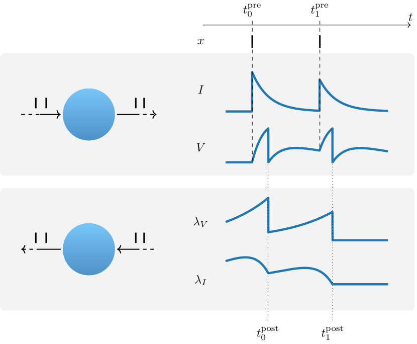
Figure 2: Forward and adjoint (backward) dynamics of a LIF neuron receiving two input spikes at $t_{1}^{pre}$ and $t_{2}^{pre}$. The membrane potential experiences two jumps, giving the post-synaptic spike times $t_{1}^{post}$ and $t_{2}^{post}$. In the computation of the adjoint dynamics, which happens backwards in time, the adjoint variable $\lambda_{V}$ experiences jumps at the two post-synaptic spike times. The gradient contributions are then computed by sampling the adjoint state at the respective pre-synaptic spike times.

3 Hardware Training Results on the Yin-Yang Dataset

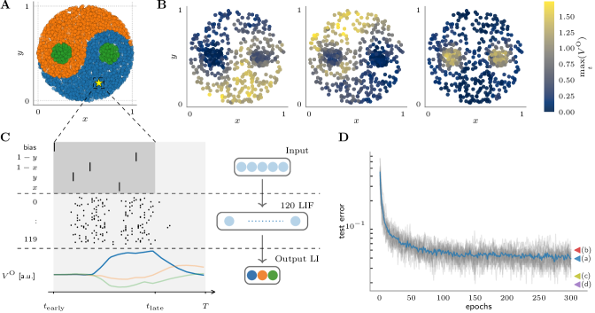
Figure 3: A Example points of Yin-Yang dataset (Kriener et al., 2022). The dataset is represented by two-dimensional points classified into one of the three classes yin (blue), yang (orange) or dot (green). B The maximum membrane values of the three output LI-neurons are used for classification and are shown for the test set after training. C Samples from the dataset are symmetrized and encoded into a time window $[t_{\text{early}},t_{\text{late}}]$. Additionally, a bias spike is added. For classification, those input spikes are projected onto a hidden layer of 120 LIF neurons. The hidden spikes are received by an output layer of 3 LI neurons. The activity and observables of the network are shown for the yellow sample in A. Spikes and membrane voltages use different timestamp clocks; we only approximately aligned the two time domains. D The test error for hardware-ITL training with EventProp on the Yin-Yang dataset is depicted and compared to other results as given in Table 1.

Type	Grad. Estimator			Loss	Acc. [%]
ANN	Backprop. (Kriener et al., 2022)			CE	97.6 ±1.5
	Backprop. (Kriener et al., 2022)			CE	85.5 ±5.8
	(frozen lower weights)
SNN	analytical (Göltz et al., 2021)	sim.		TTFS	95.9 ±0.7
	analytical (Göltz et al., 2021)	hw	$\blacktriangleleft$ (b)	TTFS	95.0 ±0.9
	EventProp (Wunderlich & Pehle, 2021)	sim.	$\blacktriangleleft$ (d)	TTFS	98.1 ±0.2
SNN	Surr. Gradient	sim.		Max	97.6 ±0.4
	Surr. Gradient	hw		Max	94.6 ±0.7
	EventProp	sim.	$\blacktriangleleft$ (c)	Max	97.9 ±0.6
	EventProp	hw	$\blacktriangleleft$ (a)	Max	96.1 ±0.8

Table 1: Test accuracies on the Yin-Yang task for ANN s and SNN s with different gradient estimators and loss definitions. For the SNN s numerical integration and hardware emulation are compared. The results marked by ‘CE’ use a cross-entropy loss, the ‘TTFS’ results are using a loss based on time-to-first-spike decoding and the ‘Max’ results are based on ‘maximum membrane value over time’. Kriener et al. (2022) use an ANN with 30 hidden neurons. Wunderlich & Pehle (2021) use a SNN with 200 hidden neurons, the results by Göltz et al. (2021) and our own results use 120 hidden neurons.

We choose the Yin-Yang dataset (Kriener et al., 2022), a two-dimensional classification task with three classes, to demonstrate the learning algorithm on BrainScaleS-2. A point $(a,b)$ in the dataset lies in the interior of the box $[0,1]\times[0,1]$ and belongs to one of three classes depending on which part of the “Yin-Yang” it belongs to. In Table 1 and Fig. 3 we report our results. Hyperparameters and training details are given in Section 6.4 and Table 3.

We compare our surrogate-gradient and EventProp implementation both in simulation and on hardware in-the-loop training. We find that in simulation both the surrogate gradient and EventProp implementation achieve comparable performance. Using the hardware-in-the loop approach to estimate gradients we achieve on average $1.5\%$ higher accuracy with the EventProp gradient estimation method and the highest observed hardware performance on this task so far, compared to previously reported results using the Fast-and-Deep gradient estimation algorithm (Göltz et al., 2021).

We use Eq. (1) to estimate the gain in information efficiency for this particular experiment on the Yin-Yang dataset. Sampling the membrane voltages of 120 hidden neurons with $500\text{\,}\mathrm{kHz}\text{/}$ over $38\text{\,}\mathrm{\SIUnitSymbolMicro s}\text{/}$ results in a total of $n_{v}=2280$ voltage samples per input datapoint. In the last epoch of the training with EventProp, we measure an average of $n_{e}=146\pm 13$ spikes in the hidden layer per input datapoint of the training set. This leads to a factor of $6.2\pm 0.5$ improvement in memory efficiency using EventProp compared to training with surrogate gradients.

4 Hardware Gradient Estimation

Since previous work (Göltz et al., 2021) had demonstrated that gradient-estimation using an analytical formula for the spike time of LIF neurons could successfully be applied to hardware in-the-loop training, we ask whether the gradient estimate computed using our method would match the analytic estimate. We find that for a simple experiment setup with one LIF neuron receiving one input spike with weight $w$ at time $t=0$, the mean of the estimated gradient of the loss function $L=t^{\mathrm{post}}$, where $t^{\mathrm{post}}$ is the spike time of the LIF neuron, agrees well with the analytical prediction (see Fig. 4).

Figure 4: Experiment setup (top), spike time (middle) acquired from runs on BrainScaleS-2 and estimated gradient (bottom) for a loss function $L=t^{\mathrm{post}}$ as a function of the weight $w$. Results for $n=50$ hardware neuron circuits are shown in light grey, the average in dashed black. The analytical result (blue line, see Fig. 5) agrees well with the hardware average.

5 Discussion

We demonstrated a gradient estimation algorithm for analog neuromorphic hardware requiring only spike observations and making no assumptions on the network topology or loss function. As such, this has the potential to enable scalable gradient estimation in large-scale neuromorphic hardware since continuous measurement of the system state would be prohibitively expensive in this case. In particular, a similar approach to the one pursued here would also apply to neuromorphic systems for which continuous sampling of the system state would be infeasible even in principle, such as ones based on novel nano-devices or photonic neuromorphic systems. While the original implementation of EventProp (Wunderlich & Pehle, 2021) relied on a custom event-based solver, we use here a PyTorch implementation and time-discretized forward- and adjoint dynamics. Such a time-discretized implementation would also be suitable for digital neuromorphic hardware. Future work will take advantage of an event-based solver to demonstrate tasks that require precise spike timing or computation on sparse data.

Although the results reported here are encouraging, further work is needed in several areas:

• We would like to demonstrate the algorithm on further tasks, particularly ones that are not feasible using surrogate-gradient-based in-the-loop training due to hardware trace-memory limitations.

• We would like to demonstrate the scalability of the algorithm by applying it on larger-scale networks, and on longer time scales.

• We would like to demonstrate the algorithm on other neuron configurations supported by the chip.

Going beyond the immediate applications of this work, we would like to use hardware observables to learn the dynamics, instead of assuming a particular model. Demonstrating the scalability of the algorithm beyond the modest size of the network considered here requires both a multi-chip experiment setup, which is currently being built, and potentially network models that account for delays. We have evaluated the EventProp algorithm itself on larger-scale convolutional feed-forward architectures with $\sim 10^{5}$ neurons and $\sim 10^{6}$ parameters and found no performance disadvantage over surrogate gradients. However, we were fundamentally limited by the small number of integration timesteps and memory constraints.

In digital neuromorphic hardware, it is relatively straightforward to simulate the implemented neuron dynamics with commodity hardware. Thus, this work can be viewed mainly as a demonstration that the temporal discretization and quantization of observables are not an obstacle to the implementation of the EventProp gradient estimation algorithm.

Our results also suggests that a fully on-device implementation of the algorithm would be possible, where the required spike time information and voltage slopes at spike times could be stored locally at each neuron circuit. Both the forward and adjoint dynamics can be realised within the analog computation paradigm and in the current form with the very similar analog circuits. Following this direction would enable scalable, energy-efficient, event-based learning in large-scale analog neuromorphic hardware.

6 Methods

6.1 Adjoint Sensitivity Analysis with Jumps

The BrainScaleS-2 system can emulate the AdEx neuron model (Gerstner & Brette, 2009) faithfully (Billaudelle et al., 2022). To illustrate how to determine paramter gradients we consider here only an adaptive leaky-integrate and fire neuron. Its equations specify a hybrid-ordinary differential equation and we use adjoint-sensitivity analysis with jumps to derive exact gradients for this model, following the approach of Wunderlich & Pehle (2021). We are considering a loss function that can depend on the spike times and voltage traces

$$L=l_{p}(t^{p})+\int_{0}^{T}l(V)\mathrm{dt}$$ (2)

more general loss functions can also be considered and indeed the max-time-loss does not follow this form. For a derivation of how the max-over-time loss can be incorporated see Wunderlich & Pehle (2021). The dynamical equations of the model are given by

$$C\dot{V} =-g_{L}(V-E_{L})-w+RI$$ (3)

$$\tau_{w}\dot{w} =a(V-E_{L})-w$$ (4)

$$\tau_{s}\dot{I} =-I.$$ (5)

Here $C$ is the membrane capacitance, $g_{L}$ the leak conductance, $E_{L}$ the leak potential, $w$ the adaptation variable, $R$ the input resistance and $\tau_{w},\tau_{s}$ are the adaptation and synaptic time constants respectively. After a change of variables $v=V-E_{L}$, we can write these equations in matrix form

$$\dot{x}=\begin{bmatrix}\dot{v}\\ \dot{w}\\ \dot{I}\end{bmatrix}=Ax=\begin{bmatrix}-\tau^{-1}_{m}&-1/C&R/C\\ -a\tau^{-1}_{w}&-\tau^{-1}_{w}&0\\ 0&0&-\tau^{-1}_{s}\end{bmatrix}\begin{bmatrix}v\\ w\\ I\end{bmatrix}.$$ (6)

When $v$ reaches a threshold $\vartheta$, then the neuron is subject to the following transition in its state:

$$\begin{bmatrix}v^{+}\\ w^{+}\\ I^{+}\end{bmatrix}=\begin{bmatrix}0&0&0\\ 0&1&0\\ 0&0&1\\ \end{bmatrix}\begin{bmatrix}v^{-}\\ w^{-}\\ I^{-}\end{bmatrix}+\begin{bmatrix}v_{r}\\ b\\ 0\end{bmatrix}.$$ (7)

If we consider a network of $n$ neurons with state vector $x$, connected by a synaptic weight matrix, then if neuron $i$ reaches its threshold the resulting transition can be written as

$$x^{+}=P^{T}_{i}TP_{i}x^{-}+(\mathbb{1}-P^{T}_{i}P_{i})x^{-}+p_{i},$$ (8)

with $P_{i}$ the projection of the $3n$ dimensional state space to the $3$ dimensional state-space of neuron $i$,

$$T=\begin{bmatrix}0&0&0\\ 0&1&0\\ 0&0&1\\ \end{bmatrix}$$ (9)

and $p_{i}$ given by the translation induced by synaptic transmission, the reset of the membrane potential and shift of the adaptation constant.

Based on this description it is easy to compute the associated adjoint sensitivity equations with jumps, as well as the corresponding parameter gradients. The adjoint equations are given by,

$$\lambda^{\prime}=\begin{bmatrix}-g_{L}/C&-a/\tau_{w}&0\\ -1/C&-1/\tau_{w}&0\\ R/C&0&-1/\tau_{s}\end{bmatrix}\lambda,$$ (10)

and their jumps are computed according to

$$(\lambda^{-})^{T}=(\lambda^{+})^{T}\left[[f^{+}-\partial_{x^{-}}\theta f^{-}]\frac{\partial_{x^{-}}j}{\partial_{x^{-}}j\dot{x}^{-}}+\partial_{x^{-}}\theta\right].$$ (11)

Here we have

$$f^{+} =A(P^{T}_{i}TP_{i}x^{-}+(\mathbb{1}-P^{T}_{i}P_{i})x^{-}+p_{i}),$$ (12)

$$f^{-} =Ax^{-},$$ (13)

$$\partial_{x^{-}}\theta =P^{T}_{i}TP_{i}+(\mathbb{1}-P^{T}_{i}P_{i}),$$ (14)

$$\partial_{x^{-}}j =\partial_{x^{-}}(a^{T}x^{-}+w)=a^{T},$$ (15)

where $A$ was defined in Eq. (6) and $a^{T}=(1,0,0)$. This simplifies the equation to

$$(\lambda^{-})^{T}=(\lambda^{+})^{T}\left[Ap_{i}\frac{a^{T}}{a^{T}\dot{x}^{-}}+P^{T}_{i}TP_{i}+(\mathbb{1}-P^{T}_{i}P_{i})\right].$$ (16)

There exists an equally simple expression for the gradient contributions to the synaptic weights $w_{ji}$ (Wunderlich & Pehle, 2021)

$$\frac{dL}{dw_{ji}}=-\tau_{s}\sum_{\mathrm{spikes\,from\,i}}(\lambda_{I})_{j}.$$ (17)

The formulas derived here simplify to the ones obtained in (Wunderlich & Pehle, 2021), if the adaptation variable $w$ is omitted. It is also possible to use the same overall approach to derive explicit adjoint equations for the full AdEx neuron model, including the case of an absolute refractory period or synaptic transmission delays. One consideration is that since the full AdEx dynamics is non-linear, the full membrane voltage trace enters the adjoint dynamics. This introduces an additional complication in the potential applicability of the method.

6.2 Software Framework

Our software stack translates the high-level SNN experiment description to a data flow graph representation, places and routes neurons and synapses on the hardware substrate, and compiles stimulus inputs, recording settings, and other runtime dynamics into an experiment program representing an equivalent experiment configuration on BrainScaleS-2, see Müller et al. (2022a) for a detailed description. The analog substrate on BrainScaleS-2 is subject to device variations, or fixed-pattern noise, that can be compensated for by calibration. At the same time, the calibration routines consider user-defined model parameters to provide an equivalent parametrization of the emulation. A complete calibration data set provides per-circuit operation point settings. The training employed in this paper only affects the digital weight parameters and is implemented as an incremental reconfiguration providing quick hardware-ITL updates. The BrainScaleS-2 hardware substrate only supports fixed-sign $6\text{\,}\mathrm{bit}\text{/}$ synapses. We allocate two hardware synapses per software weight $w_{\text{sw}}$ to support efficient signed weight matrix updates. Each software weight $w_{\text{sw}}$ is linearly scaled into a hardware-compatible range and rounded to the nearest integer value. The batched input spikes are injected into BrainScaleS-2 and the SNN is emulated for $T=$38\text{\,}\mathrm{\SIUnitSymbolMicro s}\text{/}$$ per batch entry. During emulation, spike events and neuron membrane traces can be recorded to the FPGA DRAM. The host computer reads back and post-processes the recorded data. For experiments relying on columnar ADC (CADC) membrane measurements, the membrane samples are expressed on an equidistant time grid by linear interpolation in order to be represented by a torch::Tensor with a fixed time grid and thus aligned to the PyTorch API. Additionally, the values are offset and scaled into a desired range. The spike recordings are mapped to a boolean tensor on the same time grid.

This hardware-ITL operation mode on BrainScaleS-2 is supported by hxtorch.snn (Spilger et al., 2023), a PyTorch-based (Paszke et al., 2017) library that automates and abstracts away hardware-specific procedures and provides data conversions from and to PyTorch.

6.3 Numerical Gradient Estimate

We discretize the forward and adjoint dynamics using the explicit Euler integration scheme to implement the EventProp Algorithm, which is derived in continuous time (Wunderlich & Pehle, 2021). The dynamics of the LIF neurons with exponential-shaped, current-based synapses are either computed in simulation only or can be injected from observations when training with hardware in the loop. This, together with computing the adjoint trajectories, is handled in a custom torch.autograd.Function. The complete dataflow, together with another function ensuring the correct backpropagation to the synaptic weights and the previous layer is displayed in Figure 7. The gradient estimation for a layer of LIF neurons are described in Algorithm 1.

For the backward computation we need the spike times and the time derivatives of the membrane $\dot{V}$, which are determined only by the synaptic currents $I$ at spike times. When training with hardware in the loop, synaptic currents are not accessible and need to be estimated in order to be able to calculate the jumps of the adjoint variables. We estimate the synaptic currents by numerically integrating Equation 5 while assuming ideal dynamics on hardware and use the boolean tensors, to which the spike recordings were mapped, to apply the transitions as in Equation 8.

To compare our gradient estimate from simulation to the analytical gradient, we consider the experiment setup of a LIF neuron receiving a single spike with weight $w$ as in Figure 4. For the special case of $\tau_{\text{syn}}=\tau_{\text{mem}}$, $\tau_{\text{refrac}}=0$ the explicit formula from Göltz et al. (2021) is used.

For spike time dependent losses, as for the gradient comparisons in Figure 4 and Figure 5, we need to extract spike times from dense boolean tensors. To be able to optimize on such losses, we wrote a custom torch.autograd.Function, see Figure 6. The gradient with respect to the time of a spike is backpropagated at the index, at which the spike was located in the dense boolean input tensor.

There are two sources of errors introduced by numerical implementation: Since we only evaluate spike times on a fixed time grid, the spike time changes in jumps as the synaptic weight increases. The second error source is the numerical error introduced by the integration method itself. The chosen integration scheme is only first-order accurate. As seen in Figure 5, the jumps in the spike times have a larger impact on the mismatch in the gradient estimate, relative to the analytical formula.

For decreasing integration time steps $dt$ the numerical gradient estimate converges to the analytically known gradient. Therefore, we consider forward euler integration sufficient for our experiments.

Figure 5: Spike time (top) and estimated gradient (bottom) for a loss function $L=t^{\mathrm{post}}$ as a function of the weight $w$. As the numerical integration timestep $\mathrm{dt}$ decreases the numerically estimated gradient (dashed lines) converges to analytically known gradient (solid-black line), cf. Göltz et al. (2021). Jumps in the gradient and spike time are due to the finite resolution $\mathrm{dt}$ of the time-grid, note that the gradient is changing although the spike time remains constant.

Algorithm 1 Discrete EventProp gradient estimation for a single layer of LIF neurons

0:  

  pre-synaptic spikes $\textbf{z}_{\mathrm{pre}}$,

  parameters $\bm{W}$, $\tau_{\mathrm{m}}$, $\tau_{\mathrm{s}}$, $dt$, $T$,

  optional: hardware data $(\textbf{V}_{\mathrm{hw}},\textbf{z}_{\mathrm{hw}})$

   {Forward pass}

  if no hardware data then

     $(\textbf{V}_{\mathrm{sw}},\textbf{I}_{\mathrm{sw}},\textbf{z}_{\mathrm{sw}})$ by forward euler integration of forward dynamics and jumps from $0$ to $T$, step size $dt$

  else

     Estimate $\textbf{I}_{\mathrm{hw}}$ from $\bm{W}$ and $\textbf{z}_{\mathrm{pre}}$

  end if

   {Backward pass}

  $(\bm{\lambda}_{I},\bm{\lambda}_{V})$ by forward euler integration of adjoint dynamics and jumps from $T$ to $0$, step size $dt$

  

  $\frac{\mathrm{d}L}{\mathrm{d}\bm{W}}=-\tau_{\mathrm{s}}\bm{\lambda}_{I}^{\top}\textbf{z}_{\mathrm{pre}}$, $\frac{\mathrm{d}L}{\mathrm{d}\textbf{z}_{\mathrm{pre}}}=(\bm{\lambda}_{V}-\bm{\lambda}_{I})\bm{W}$

6.4 Training Details

The four values $(a,b,1-a,1-b)$ for each sample of the Yin-Yang dataset are translated into spike times using a latency encoding inside the time interval $[t_{\text{early}},t_{\text{late}}]$. Additionally a bias spike is added at $t_{\text{bias}}$, which serves as a fifth input spike and is the same for every data point. Those times are then mapped as events onto a boolean tensor on the desired time grid.

The feed-forward network consists of a hidden layer with 120 LIF neurons and an output layer of 3 LI neurons, one for each class. The loss we use is composed of two terms $L=L_{1}+L_{2}$. The first and main term is a max-over-time loss

$$L_{1} =-\frac{1}{N_{\text{batch}}}\sum_{n=1}^{N_{\text{batch}}}\log\frac{\exp\left(\max_{t}V^{\text{O}}_{n,y_{n}}(t)\right)}{\sum_{c=1}^{C}\exp\left(\max_{t}V^{\text{O}}_{n,c}(t)\right)},$$ (18)

with time $t$, the voltages of the output layer neurons $V^{\text{O}}$, the target $y$, the batch size $N_{\text{batch}}$ and the number of classes $C$. Additionally, to prevent the amplitudes from being to high, we add a regularization term

$$L_{2} =\alpha\cdot\frac{1}{N_{\text{batch}}\,C}\sum_{n=1}^{N_{\text{batch}}}\sum_{c=1}^{C}\left(\max_{t}V_{n}^{\text{O}}(t)\right)^{2},$$ (19)

where $\alpha$ is a scaling factor to adjust the influence of this amplitude regularization.

When using BrainScaleS-2 ITL training, we repeat the input per sample five times, ultimately giving us 25 input streams per data point. The hidden weights are initialized as an $n_{\text{hidden}}\times 5$ matrix and are then also repeated 5 times along the input dimension, resulting in a $n_{\text{hidden}}\times 25$ weight matrix. This gives us an equivalent of an increase in synaptic efficacy without changing the target model parameters and underlying calibration data set.

Comparing the gradients of the output layer weights to those of the hidden layer weights, the gradients differ by multiple orders of magnitude. To counteract this, we scale the the weight gradients computed by the EventProp algorithm with a factor $1/\tau_{s}$, which was necessary to obtain the results on the Yin-Yang dataset.

Author Contributions

CP: Conceptualization, formal analysis, writing — original draft, writing — reviewing & editing; LB: Validation, formal analysis, investigation, visualization, writing — original draft, writing — reviewing & editing; EA: Methodology, software, resources, writing — original draft, writing — reviewing & editing; EM: Methodology, software, resources, writing — original draft, writing — reviewing & editing, supervision; JS: Supervision, funding acquisition, writing — reviewing & editing.

Funding

This work has received funding from the EC Horizon 2020 Framework Programme under grant agreements 785907 (HBP SGA2) and 945539 (HBP SGA3), the Deutsche Forschungsgemeinschaft (DFG, German Research Foundation) under Germany’s Excellence Strategy EXC 2181/1-390900948 (the Heidelberg STRUCTURES Excellence Cluster), the German Federal Ministry of Education and Research under grant number 16ES1127 as part of the Pilotinnovationswettbewerb ‘Energieeffizientes KI-System’, the Helmholtz Association Initiative and Networking Fund [Advanced Computing Architectures (ACA)] under Project SO-092, as well as from the Manfred Stärk Foundation, and the Lautenschläger-Forschungspreis 2018 for Karlheinz Meier.

Appendix A Neuromorphic Architectures

Arch	Hardware Model	Modeling Paradigm
SpiNNaker 1	soft digital	bio. SNN; distributed programming
(Furber et al., 2012)	(Rhodes et al., 2018; Rowley et al., 2019; Galluppi et al., 2015, 2012)
SpiNNaker 2	soft digital	bio. SNN; distributed programming; ANN
(Mayr et al., 2019)	(Rostami et al., 2022; Yan et al., 2019)
Loihi 1	flexible digital	bio. & ML-friendly SNN; ANN
(Davies et al., 2018)	(Rueckauer et al., 2021; DeWolf et al., 2020; Lin et al., 2018)
Loihi 2	flexible digital	bio. & ML-friendly SNN; ANN
(Orchard et al., 2021)	(loi, 2021)
TrueNorth	hard digital	bio. SNN; ANN
(Merolla et al., 2014)	(Amir et al., 2013)
ODIN	hard digital	bio. SNN
(Frenkel et al., 2018)	(Frenkel et al., 2018)
Tianjic	hard digital	bio. SNN; ANN
(Pei et al., 2019)	(Ji et al., 2016)
BrainScaleS-1	physical	bio. SNN
(Schemmel et al., 2010)	(Müller et al., 2022b)
BrainScaleS-2	physical	bio. and ML-friendly SNN; ANN
(Pehle et al., 2022; Billaudelle et al., 2022)	(Müller et al., 2022a; Spilger et al., 2020, 2023)
ROLLS	physical	bio. SNN
(Qiao et al., 2015)	(Stefanini et al., 2014)
DynapSE	physical	SNN
(Moradi et al., 2018)	(dyn, 2021)
Neurogrid	physical	SNN
(Benjamin et al., 2014)	(Voelker et al., 2017)

Table 2: Overview of neuromorphic chip architectures: At one end of the spectrum, programmable standard processors offer modeling flexibility that can come close to software simulations while maintaining higher efficiency. On the other end of the spectrum, analog circuits typically offer high energy efficiency or speed, but this is typically based on a trade-off in modeling flexibility or precision. Both digital and analog implementations offer many different optimization options. Some systems focus on biological SNN operation, while others support machine-learning-inspired training or classical ANN operation.

Appendix B Spike time decoder

⬇

class ToSpikeTimes(torch.autograd.Function):

\pardef forward(

ctx,

spike_input: torch.Tensor,

spike_count: torch.Tensor,

dt: float) -> torch.Tensor:

batch_size, time_size, out_size = spike_input.shape

indexed_spike_input =

spike_input * torch.arange(1, time_size + 1)[None, :, None] - 1.0

indexed_spike_input[indexed_spike_input == -1.0] = float(”inf”)

if spike_count < time_size:

spike_indices = torch.sort(

indexed_spike_input, dim=1).values[:, :spike_count]

else:

spike_indices = torch.sort(

indexed_spike_input, dim=1).values[:, :time_size]

ctx.save_for_backward(spike_indices, spike_input)

ctx.shape = spike_input.shape

return spike_indices * dt

\pardef backward(

ctx,

grad_output: torch.Tensor) -> Tuple[torch.Tensor, None, None]:

(spike_indices, spike_input) = ctx.saved_tensors

batch_size, spike_count, out_size = spike_indices.shape

noninf_spike_indices = spike_indices.flatten() != float(”inf”)

\pargrad_input = torch.zeros_like(spike_input, dtype=torch.float)

\pargrad_input_indices = (

torch.arange(batch_size).repeat_interleave(out_size).repeat(

spike_count)[noninf_spike_indices],

spike_indices.flatten()[noninf_spike_indices].type(torch.long),

torch.arange(out_size).repeat(batch_size).repeat(

spike_count)[noninf_spike_indices],

)

\pargrad_input[grad_input_indices] = \ - 1.0 * grad_output.flatten()[noninf_spike_indices]

\parreturn grad_input, None, None

Figure 6: Custom torch.autograd.Function to convert boolean tensors holding spikes into spike times in a backpropagation-compatible fashion. The argument spike_count adjusts how many of each neurons spikes are retrieved. If a neuron does spike fewer times than specified by spike_count, the spike times are set to floating-point infinity. The backpropagation happens by injecting the gradient with respect to a spike time at the corresponding position, at which the spike occurred in the boolean input tensor, with a negative sign. All other entries remain to be zero.

Appendix C Training Parameters

Parameter	EventProp	SuperSpike
$\tau_{\text{mem}}$	$6\text{\,}\mathrm{\SIUnitSymbolMicro s}\text{/}$	$6\text{\,}\mathrm{\SIUnitSymbolMicro s}\text{/}$
$\tau_{\text{syn}}$	$6\text{\,}\mathrm{\SIUnitSymbolMicro s}\text{/}$	$6\text{\,}\mathrm{\SIUnitSymbolMicro s}\text{/}$
size input	5	5
size hidden layer	120	120
size output layer	3	3
weight init [mean, stdev]
hidden	[0.2, 0.2]	[0.001, 0.15]
output	[0.01, 0.1]	[0.0, 0.1]
$dt$	$0.5\text{\,}\mathrm{\SIUnitSymbolMicro s}\text{/}$	$0.5\text{\,}\mathrm{\SIUnitSymbolMicro s}\text{/}$
$t_{\text{bias}}$	$2\text{\,}\mathrm{\SIUnitSymbolMicro s}\text{/}$	$2\text{\,}\mathrm{\SIUnitSymbolMicro s}\text{/}$
$t_{\text{early}}$	$2\text{\,}\mathrm{\SIUnitSymbolMicro s}\text{/}$	$2\text{\,}\mathrm{\SIUnitSymbolMicro s}\text{/}$
$t_{\text{late}}$	$26\text{\,}\mathrm{\SIUnitSymbolMicro s}\text{/}$	$26\text{\,}\mathrm{\SIUnitSymbolMicro s}\text{/}$
$t_{\text{sim}}$	$38\text{\,}\mathrm{\SIUnitSymbolMicro s}\text{/}$	$38\text{\,}\mathrm{\SIUnitSymbolMicro s}\text{/}$
training epochs	300	300
batch size	50	100
optimizer	Adam	Adam
Adam parameter $\beta$	(0.9, 0.999)	(0.9, 0.999)
Adam parameter $\epsilon$	$10^{-8}$	$10^{-8}$
learning rate	0.0005	0.001
lr-scheduler	StepLR	StepLR
lr-schedule step size	50	50
lr-scheduler $\gamma$	0.5	0.5
readout reg.	0.0004	0.0004

Table 3: Parameters of neuron dynamics, network and training used to produce the hardware-in-the-loop results on the Yin-Yang dataset using EventProp and SuperSpike surrogate gradients as shown in Figure 3 and Table 1.

Parameter	EventProp	SuperSpike
size input	5	5
size hidden layer	120	120
size output layer	3	3
weight init [mean, stdev]
hidden	[1.0, 0.4]	[1.0, 0.4]
output	[0.01, 0.1]	[0.01, 0.1]
$dt$ $\left[\tau_{\text{s}}\right]$	$0.01\text{\,}\text{/}$	$0.01\text{\,}\text{/}$
$t_{\text{bias}}$ $\left[\tau_{\text{s}}\right]$	$0\text{\,}\text{/}$	$0\text{\,}\text{/}$
$t_{\text{early}}$ $\left[\tau_{\text{s}}\right]$	$0\text{\,}\text{/}$	$0\text{\,}\text{/}$
$t_{\text{late}}$ $\left[\tau_{\text{s}}\right]$	$4\text{\,}\text{/}$	$4\text{\,}\text{/}$
$t_{\text{sim}}$ $\left[\tau_{\text{s}}\right]$	$6\text{\,}\text{/}$	$6\text{\,}\text{/}$
training epochs	200	200
batch size	25	50
optimizer	Adam	Adam
Adam parameter $\beta$	(0.9, 0.999)	(0.9, 0.999)
Adam parameter $\epsilon$	$10^{-8}$	$10^{-8}$
learning rate	0.0005	0.0005
lr-scheduler	StepLR	StepLR
lr-schedule step size	50	50
lr-scheduler $\gamma$	0.5	0.5
readout reg.	0.0	0.0

Table 4: Parameters of neuron dynamics, network and training used to produce the software-only results on the Yin-Yang dataset using EventProp and SuperSpike surrogate gradients as listed Table 1. We chose $\tau_{\text{s}}=\tau_{\text{m}}$ and times are given in units of $\tau_{\text{s}}$.

Appendix D EventProp Dataflow

Figure 7: Dataflow occurring during hardware-in-the-loop training. EventPropSynapse returns the product of the input spikes and the weight $w$ stacked on top of an empty tensor with same shape. EventPropNeuron either returns the hardware observations or, if those are not present, computes the forward trajectories in simulation. In the backward pass, the adjoint dynamics are computed using the stored spikes from the forward-call and a stacked tensor consisting of $\tau_{\text{s}}\lambda_{\text{I}}$ and $(\lambda_{\text{I}}-\lambda_{\text{V}})$ is returned. Note that returning these stacked tensors is only possible due to the output of EventPropSynapse already being a stacked tensor with same shape. In backward direction, EventPropSynapse backpropagates $\tau_{\text{s}}\lambda_{\text{I}}^{\top}z_{\text{pre}}$, the gradient with respect to the weight according to the EventProp algorithm (Wunderlich & Pehle, 2021), and $(\lambda_{\text{I}}-\lambda_{\text{V}})w$, the gradient with respect to the pre-synaptic spikes.

References

- dyn (2021) Nice workshop 2021: A tiny spiking neural network on dynap-se1 board simulator, 2021. URL https://code.ini.uzh.ch/yigit/NICE-workshop-2021.
- loi (2021) Intel: Announcement of loihi-2 and new software framework. https://www.intel.com/content/www/us/en/newsroom/news/intel-unveils-neuromorphic-loihi-2-lava-software.html, 2021. https://github.com/lava-nc/.
- Amir et al. (2013) Amir, A., Datta, P., Risk, W. P., Cassidy, A. S., Kusnitz, J. A., Esser, S. K., Andreopoulos, A., Wong, T. M., Flickner, M., Alvarez-Icaza, R., McQuinn, E., Shaw, B., Pass, N., and Modha, D. S. Cognitive computing programming paradigm: A corelet language for composing networks of neurosynaptic cores. In The 2013 International Joint Conference on Neural Networks (IJCNN), pp. 1–10. IEEE, 2013.
- Arnold et al. (2022) Arnold, E., Böcherer, G., Müller, E., Spilger, P., Schemmel, J., Calabrò, S., and Kuschnerov, M. Spiking neural network equalization on neuromorphic hardware for IM/DD optical communication. In European Conference on Optical Communication (ECOC) 2022, pp. Th1C.5. Optica Publishing Group, June 2022. URL https://opg.optica.org/abstract.cfm?URI=ECEOC-2022-Th1C.5.
- Benjamin et al. (2014) Benjamin, B. V., Gao, P., McQuinn, E., Choudhary, S., Chandrasekaran, A. R., Bussat, J.-M., Alvarez-Icaza, R., Arthur, J. V., Merolla, P. A., and Boahen, K. Neurogrid: A mixed-analog-digital multichip system for large-scale neural simulations. Proceedings of the IEEE, 102(5):699–716, 2014.
- Billaudelle et al. (2022) Billaudelle, S., Weis, J., Dauer, P., and Schemmel, J. An accurate and flexible analog emulation of AdEx neuron dynamics in silicon. arXiv preprint, 2022. doi: 10.48550/arXiv.2209.09280.
- Cramer et al. (2022) Cramer, B., Billaudelle, S., Kanya, S., Leibfried, A., Grübl, A., Karasenko, V., Pehle, C., Schreiber, K., Stradmann, Y., Weis, J., et al. Surrogate gradients for analog neuromorphic computing. Proceedings of the National Academy of Sciences, 119(4), 2022.
- Davies et al. (2018) Davies, M., Srinivasa, N., Lin, T.-H., Chinya, G., Cao, Y., Choday, S. H., Dimou, G., Joshi, P., Imam, N., Jain, S., et al. Loihi: A neuromorphic manycore processor with on-chip learning. IEEE Micro, 38(1):82–99, 2018. doi: 10.1109/MM.2018.112130359.
- DeWolf et al. (2020) DeWolf, T., Jaworski, P., and Eliasmith, C. Nengo and low-power ai hardware for robust, embedded neurorobotics. Frontiers in Neurorobotics, 14, 2020. ISSN 1662-5218. doi: 10.3389/fnbot.2020.568359.
- Esser et al. (2016) Esser, S. K., Merolla, P. A., Arthur, J. V., Cassidy, A. S., Appuswamy, R., Andreopoulos, A., Berg, D. J., McKinstry, J. L., Melano, T., Barch, D. R., di Nolfo, C., Datta, P., Amir, A., Taba, B., Flickner, M. D., and Modha, D. S. Convolutional networks for fast, energy-efficient neuromorphic computing. Proceedings of the National Academy of Sciences, 113(41):11441–11446, 2016. ISSN 0027-8424. doi: 10.1073/pnas.1604850113.