Estimation of coefficients for periodic autoregressive model with additive noise - a finite-variance case

Abstract

Periodic autoregressive (PAR) time series is considered as one of the most common models of second-order cyclostationary processes. In real applications, the signals with periodic characteristics may be disturbed by additional noise related to measurement device disturbances or to other external sources. The known estimation techniques for PAR models assume noise-free model, thus may be inefficient for such cases. In this paper, we propose four estimation techniques for the noise-corrupted finite-variance PAR models. The methodology is based on Yule-Walker equations utilizing the autocovariance function. Thus, it can be used for any type of the finite-variance additive noise. The presented simulation study clearly indicates the efficiency of the proposed techniques, also for extreme case, when the additive noise is a sum of the Gaussian additive noise and additive outliers. This situation corresponds to the real applications related to condition monitoring area which is a main motivation for the presented research.

1 Introduction

Periodic autoregressive (PAR) time series is considered as one of the most common cyclostationary processes, [1]. The second-order cyclostationary processes (called also periodically correlated, PC) are useful for the description of the systems with the measurements having a periodically non-stationary random structure, [2]. This behaviour is ubiquitous in various areas of interests, including hydrology [1, 3], climatology and meteorology [4, 5], and many others, see e.g, [6, 7]. The special attention we need to pay to the condition monitoring of mechanical systems with rotating or reciprocating elements, where signals are non-stationary but – in a natural way – cyclic [8].
The main features characterizing the cyclostationary behaviour finite-variance distributed signals are the autocovariance or autocorrelation functions (denoted as ACVF and ACF, respectively). Thus, most of the algorithms for cyclostationary signals utilize empirical counterparts of ACVF and ACF in time and frequency domains, see e.g. [9, 10].
The analyzed in this paper PAR models are considered as the natural generalization of the popular autoregressive moving average (ARMA) time series [11], where the constant parameters are replaced by the periodic deterministic functions. Moreover, the PAR models can be considered as the multidimensional AR time series with the dimension equal to the period. We mention, the ARMA time series (in one- and multi-dimensional versions) are often used in various engineering applications in order to build the model of real system based on measured data [12]. However, if the analyzed system is operating in time-varying conditions, the coefficients of ARMA model are also time-varying, in particular – periodic. Thus, in the mechanical systems, the PARMA (and in particular PAR) models were suggested as an interesting approach for mechanical systems operating in cyclic load/speed variation, [13].
There are known various estimation methods dedicated for finite-variance PAR model’s parameters. The most known technique is the Yule-Walker-based approach using the time-dependent ACVF [14]. For other techniques see e.g., [15, 16, 17, 18, 19]. All of the mentioned above estimation methods assume the ideal case, namely that the analyzed signal corresponds to the ”pure” model without any additional disturbances. However, in the real applications, this situation seldom occurs and in practice the measured signal is always noise-corrupted. The additional noise may be related to measurement device disturbances or to other sources influencing the observations. This problem was extensively discussed for the noise-corrupted ARMA-type models for different types of additive noise, see e.g., [20, 21, 22, 23, 24, 25]. The problem was also considered for the multidimensional ARMA time series, see [26]. The characterization of noise-corrupted PARMA models is also discussed in the literature. However, the main attention is paid to the special case of the additive noise, namely additive outliers (i.e., independent identically distributed (i.i.d.) observations with large values appearing with a given probability), see e.g. [27, 28, 29, 30, 31]. The algorithms do not take into consideration the existence of the additive disturbances but utilize the robust estimators of the classical statistics (like ACVF in the Yule-Walker method) in order to reduce the impact of large observations visible in the signal. The additive noise may have a much wider sense than just several outliers. The disturbance may be a random process with Gaussian or non-Gaussian distribution and the mentioned outliers as well. All these factors strongly depend on the modelled system. Here, as a potential application we consider the modelling of vibration data from complex mechanical systems with time-varying periodic characteristics.
In this paper, we consider the PAR models with general finite-variance distributed additive noise and propose four estimation algorithms for their parameters. All of the introduced techniques take into account the existence of the additive noise and can be also used in the case of the additive outliers occurrence. The proposed approaches do not assume any specific distribution of the data, thus in this sense, they are universal for finite-variance case. The presented simulation study for PAR models with Gaussian additive noise clearly indicates the justification for the inclusion of the existence of the additive noise in the estimation algorithms. The efficiency of the new techniques is compared with the classical Yule-Walker technique (without the assumption of the additive noise existence) for the PAR model estimation. By Monte Carlo simulations, we have demonstrated that the classical Yule-Walker estimator is biased in contrast to the new algorithms. We also discuss the case when the additive noise is a sequence of additive outliers. The received results confirm that the proposed techniques can also be used in this case and outperform the classical approach. The most practical case considered in this paper is the PAR model with additive noise being a sum of two sequences, namely Gaussian additive noise and additive outliers. The presence of the Gaussian additive noise is very intuitive in practical situations. Most of the signal models in metrology assume the presence of additive noise related to sensor, signal discretization, data transmission, etc. Additive outliers might be related to electromagnetic disturbances in measurement systems, specific technological processes carried out by machines like cutting, crushing, sieving, pumping, compressing, or any rapid, transient phenomena. The presented results for Monte Carlo simulations indicate the efficiency of the introduced techniques also in this case.
The approaches proposed here may be seen as simple extension of estimation techniques for AR [20, 21] to PAR models (both with additive noise). It should be highlighted that the classical framework for pure PAR model identification in case of additive noise becomes insufficient/non-effective [32, 33]. Thus, each step (model order and period identification, model coefficients estimation and validation of the model) should be redefined for additive noise case. In this paper, we focus on model coefficients estimation only as in some practical applications (i.e. machine condition monitoring under cyclic load/speed) the model order and the period may be assumed based on some mechanical properties of the modelled system. The proposed four algorithms do not depend on the application and they constitute a novel PAR modelling framework with presence of additive (Gaussian/non-Gaussian) noise. Our parallel work is related to model order, period and residuals identification to complete the whole approach.
The rest of the paper is organized as follows: in Section 2 we introduce the model. In Section 3, we describe four new estimation techniques for the noise-corrupted PAR model estimation. In Section 4, we present the simulation studies related to the PAR model with Gaussian additive noise. In Section 5, we provide the analysis of the simulated signals corresponding to the PAR model with additive outliers. Last section concludes the paper and presents the future study.

2 Definition of the model

The periodic autoregressive model with additive noise (called also noise-corrupted PAR model) is defined as follows

$$Y_{t}=X_{t}+Z_{t},~{}t\in\mathbb{Z},$$ (1)

where $\{X_{t}\}$ is the periodic autoregressive time series of order $p\in\mathbb{N}$ and period $T\in\mathbb{N}$ defined below. It is assumed that innovations of the PAR($p$) model (denoted further as $\{\xi_{t}\}$) and the additive noise $\{Z_{t}\}$ constitute sequences of i.i.d. random variables with zero mean and constant variances denoted further as $\sigma_{\xi}^{2}$ for the innovations of the PAR($p$) model and $\sigma_{Z}^{2}$ for the additive noise, respectively. Additionally, we consider the case when the sequences $\{X_{t}\}$ and $\{Z_{t}\}$ are independent. We remind, the sequence $\{X_{t}\}$ is a second-order PAR($p$) ($p\in\mathbb{N}$) model with period $T\in\mathbb{N}$ when it satisfies the following equation, [34]

$$X_{t}-\phi_{1}(t)X_{t-1}-\cdots-\phi_{p}(t)X_{t-p}=\xi_{t},$$ (2)

the scalars $\{\phi_{i}(t),~{}i=1,\cdots,p\}$ are periodic in $t$ with the same period $T$. In the classical version, $\{\xi_{t}\}$ is considered as a sequence of Gaussian distributed random variables. In our simulation studies, we also consider this case. However, all presented analysis are also valid for any finite variance distribution of the innovation series.

Putting $t=nT+v$, where $n\in\mathbb{Z},\,v=1,2,\cdots,T$ one can express the PAR($p$) model in the following form

$$X_{nT+v}-\phi_{1}(v)X_{nT+v-1}-\cdots-\phi_{p}(v)X_{nT+v-p}=\xi_{nT+v}.$$ (3)

Multiplying Eq. (3) by $X_{nT+v-1},\cdots,X_{nT+v-p}$ for each $v=1,2,\cdots,T$ and taking the expected value of both sides of the above equations one obtains the following system of equations

$$\mathbf{\Gamma}^{X}_{v}\mathbf{\Phi}_{v}=\mathbf{\gamma}^{X}_{v},$$ (4)

where $\mathbf{\Phi}_{v}=[\phi_{1}(v),\cdots,\phi_{p}(v)]^{\prime}$, $\mathbf{\Gamma}^{X}_{v}$ is a $p\times p$ matrix of elements defined as follows

$$(\mathbf{\Gamma}^{X}_{v})_{i,j}=\gamma^{X}(v-i,j-i),$$ (5)

for $\gamma^{X}(w,k)=\mathbb{E}X_{nT+w}X_{nT+w-k}$ and

$$\mathbf{\gamma}^{X}_{v}=[\gamma^{X}(v,1),\cdots,\gamma^{X}(v,p)]^{\prime}.$$ (6)

Analogously, the same procedure starting with the multiplication by $X_{nT+v}$ yields the following expression

$$\gamma^{X}(v,0)-\mathbf{\gamma}_{v}^{X\prime}\mathbf{\Phi}_{v}=\sigma^{2}_{\xi}.$$ (7)

The systems defined by Eqs. (4) and (7) are also known as low-order Yule-Walker equations. However, we can also consider high-order Yule-Walker equations which are constructed in a similar manner. The only difference is that during the first step we multiply Eq. (3) by $X_{nT+v-(p+1)},\cdots,X_{nT+v-(p+s)}$, where $s$ is a desired number of equations. As a result, for each $v=1,2,\cdots,T$ we obtain the following system

$${}_{s}\tilde{\mathbf{\Gamma}}^{X}_{v}\mathbf{\Phi}_{v}={}_{s}\tilde{\mathbf{\gamma}}^{X}_{v},$$ (8)

where ${}_{s}\tilde{\mathbf{\Gamma}}^{X}_{v}$ is a $s\times p$ matrix of elements

$$({}_{s}\tilde{\mathbf{\Gamma}}^{X}_{v})_{i,j}=\gamma^{X}(v-j,p+i-j),$$ (9)

and:

$${}_{s}\tilde{\mathbf{\gamma}}^{X}_{v}=[\gamma^{X}(v,p+1),\cdots,\gamma^{X}(v,p+s)]^{\prime}.$$ (10)

Although the presented Yule-Walker equations were derived for the pure PAR($p$) model $\{X_{t}\}$, they are also useful for the noise-corrupted time series given in Eq. (1). The periodic autocovariance of $\{Y_{t}\}$ is

$$\gamma^{Y}(w,k)=\begin{cases}\gamma^{X}(w,k)+\sigma^{2}_{Z}&\text{$k=0$},\\ \gamma^{X}(w,k)&\text{$k\neq 0$}.\end{cases}$$ (11)

Using the same notation as for $\{X_{t}\}$ time series, we define $\mathbf{\Gamma}^{Y}_{v}$ and $\mathbf{\gamma}^{Y}_{v}$ (see corresponding Eqs. (5) and (6)). Because, from Eq. (11), $\gamma^{Y}(v,k)$ and $\gamma^{X}(v,k)$ are not equal only when $k=0$, thus we have $\mathbf{\gamma}^{Y}_{v}=\mathbf{\gamma}^{X}_{v}$. Moreover, the following relation holds

$$\mathbf{\Gamma}^{Y}_{v}=\mathbf{\Gamma}^{X}_{v}+\sigma^{2}_{Z}\mathbf{I}_{p}.$$ (12)

Hence, for each $v=1,2,\cdots,T$, one can rewrite the low-order Yule-Walker equations given in (4) as follows

$$(\mathbf{\Gamma}^{Y}_{v}-\sigma^{2}_{Z}\mathbf{I}_{p})\mathbf{\Phi}_{v}=\mathbf{\gamma}^{Y}_{v},$$ (13)

and similarly Eq. (7) as

$$\gamma^{Y}(v,0)-\mathbf{\Phi}_{v}^{\prime}\mathbf{\gamma}^{Y}_{v}=\sigma^{2}_{\xi}+\sigma^{2}_{Z}.$$ (14)

For high-order Yule-Walker equations, similarly, let us define ${}_{s}\tilde{\mathbf{\Gamma}}^{Y}_{v}$ as in Eq. (9) and ${}_{s}\tilde{\mathbf{\gamma}}^{Y}_{v}$ as in Eq. (10). Because ${}_{s}\tilde{\mathbf{\Gamma}}^{X}_{v}$ and ${}_{s}\tilde{\mathbf{\gamma}}^{X}_{v}$ do not contain any elements of the form $\gamma^{X}(w,0)$, we can replace each element $\gamma^{X}(w,k)$ with $\gamma^{Y}(w,k)$. Hence, we have ${}_{s}\tilde{\mathbf{\Gamma}}^{Y}_{v}={}_{s}\tilde{\mathbf{\Gamma}}^{X}_{v}$ and ${}_{s}\tilde{\mathbf{\gamma}}^{Y}_{v}={}_{s}\tilde{\mathbf{\gamma}}^{X}_{v}$. In other words, for each $v=1,2,\cdots,T$, for the process $\{Y_{t}\}$ we have the same form of high-order Yule-Walker equations as before (see Eq. (8))

$${}_{s}\tilde{\mathbf{\Gamma}}^{Y}_{v}\mathbf{\Phi}_{v}={}_{s}\tilde{\mathbf{\gamma}}^{Y}_{v}.$$ (15)

3 Estimation methods for PAR model with additive noise

In the proposed algorithms we use the following notations

$$\hat{\gamma}^{Y}(w,k)=\frac{1}{N}\sum_{n=l}^{r}y_{nT+w}y_{nT+w-k},$$ (16)

where $y_{1},y_{2},\cdots,y_{NT}$ is a zero-mean signal and

$$l=\max\left(\left\lceil\frac{1-w}{T}\right\rceil,\left\lceil\frac{1-(w-k)}{T}\right\rceil\right),$$

$$r=\min\left(\left\lfloor\frac{NT-w}{T}\right\rfloor,\left\lfloor\frac{NT-(w-k)}{T}\right\rfloor\right),$$ (17)

$$\hat{\mathbf{\Phi}}_{v}=[\hat{\phi}_{1}(v),\cdots,\hat{\phi}_{p}(v)]^{\prime}.$$ (18)

In addition, $\hat{\mathbf{\Gamma}}^{Y}_{v}$ is a $p\times p$ matrix of the following elements

$$(\hat{\mathbf{\Gamma}}^{Y}_{v})_{i,j}=\hat{\gamma}^{Y}(v-i,j-i),~{}~{}i,j=1,2,\cdots,p.$$ (19)

$$\hat{\mathbf{\gamma}}^{Y}_{v}=[\hat{\gamma}^{Y}(v,1),\cdots,\hat{\gamma}^{Y}(v,p)]^{\prime}$$ (20)

while ${}_{s}\hat{\tilde{\mathbf{\Gamma}}}^{Y}_{v}$ is a $s\times p$ matrix of the following elements

$$({}_{s}\hat{\tilde{\mathbf{\Gamma}}}^{Y}_{v})_{i,j}=\hat{\gamma}^{Y}(v-j,p+i-j),$$ (21)

where $i=1,2,\cdots,s$, $j=1,2,\cdots,p$. Moreover,

$${}_{s}\hat{\tilde{\mathbf{\gamma}}}^{Y}_{v}=[\hat{\gamma}^{Y}(v,p+1),\cdots,\hat{\gamma}^{Y}(v,p+s)]^{\prime}.$$ (22)

3.1 Method 1 – higher-order Yule-Walker algorithm

The first proposed method (called M1) is a generalization of the approach presented in [35] for all orders $p$ of the considered model. It is based on high-order Yule-Walker equations for the noise-corrupted process $\{Y_{t}\}$. To obtain the vector of estimated coefficients $\hat{\mathbf{\Phi}}_{v}$ in a given season $v=1,2,\cdots,T$, one can use the system given in Eq. (15) for $s=p$ and replace all terms of the form $\gamma^{Y}(w,k)$ with their empirical counterparts $\hat{\gamma}^{Y}(w,k)$. In other words, for each $v=1,2,\cdots,T$, one should solve the following system of equations

$${}_{p}\hat{\tilde{\mathbf{\Gamma}}}^{Y}_{v}\hat{\mathbf{\Phi}}_{v}={}_{p}\hat{\tilde{\mathbf{\gamma}}}^{Y}_{v},$$ (23)

To obtain the estimators for $\sigma^{2}_{\xi}$ and $\sigma^{2}_{Z}$, one can use Eq. (14) and the first equation of the system given in Eq. (13)

$$\hat{\gamma}^{Y}(v,0)-\hat{\mathbf{\gamma}}^{Y\prime}_{v}\hat{\mathbf{\Phi}}_{v}=\hat{\sigma}^{2}_{\xi}(v)+\hat{\sigma}^{2}_{Z}(v),$$ (24)

$$\hat{\gamma}^{Y}(v,1)-\hat{\mathbf{\Gamma}}^{Y}_{v,1}\hat{\mathbf{\Phi}}_{v}=-\hat{\sigma}^{2}_{Z}(v)\hat{\phi}_{1}(v),$$ (25)

where $\hat{\mathbf{\Gamma}}^{Y}_{v,1}=[\hat{\gamma}^{Y}(v-1,0),\cdots,\hat{\gamma}^{Y}(v-1,p-1)]$ and $\hat{\sigma}^{2}_{\xi}(v)$, $\hat{\sigma}^{2}_{Z}(v)$ are estimators of $\sigma^{2}_{\xi}(v)=\mathbb{E}\xi_{nT+v}^{2}$ and $\sigma^{2}_{Z}(v)=\mathbb{E}Z_{nT+v}^{2}$, respectively. From Eq. (25) we can easily calculate the $\hat{\sigma}^{2}_{Z}(v)$

$$\hat{\sigma}^{2}_{Z}(v)=\frac{\hat{\mathbf{\Gamma}}^{Y}_{v,1}\hat{\mathbf{\Phi}}_{v}-\hat{\gamma}^{Y}(v,1)}{\hat{\phi}_{1}(v)},$$ (26)

and put it into Eq. (24) to obtain $\hat{\sigma}^{2}_{\xi}(v)$. Because we assume that $\sigma^{2}_{\xi}$ and $\sigma^{2}_{Z}$ are not dependent on $v$, finally we take

$$\hat{\sigma}^{2}_{\xi}=\frac{1}{T}\sum_{v=1}^{T}\hat{\sigma}^{2}_{\xi}(v),\quad\hat{\sigma}^{2}_{Z}=\frac{1}{T}\sum_{v=1}^{T}\hat{\sigma}^{2}_{Z}(v).$$ (27)

The complete algorithm for the first method is presented in Algorithm 1.

Algorithm 1 Method M1

1:For each $v=1,\cdots,T$:

1. Construct ${}_{p}\hat{\tilde{\mathbf{\Gamma}}}^{Y}_{v}$ (Eq. (21)) and ${}_{p}\hat{\tilde{\mathbf{\gamma}}}^{Y}_{v}$ (Eq. (22)).

2. Compute $\hat{\mathbf{\Phi}}_{v}=(_{p}\hat{\tilde{\mathbf{\Gamma}}}^{Y}_{v})^{-1}{}_{p}\hat{\tilde{\mathbf{\gamma}}}^{Y}_{v}$.

3. Compute $\hat{\sigma}^{2}_{Z}(v)$ and $\hat{\sigma}^{2}_{\xi}(v)$ (Eq. (26) and Eq. (24)).

2:Compute $\hat{\sigma}^{2}_{Z}=1/T\sum_{v=1}^{T}\hat{\sigma}^{2}_{Z}(v)$.

3:Compute $\hat{\sigma}^{2}_{\xi}=1/T\sum_{v=1}^{T}\hat{\sigma}^{2}_{\xi}(v)$.

3.2 Method 2 – errors-in-variables method

The second proposed approach (called later M2) is based on the method presented in [21] for noise-corrupted autoregressive models. Similar as approach M1, this estimation procedure will be defined independently for each season $v=1,2,\cdots,T$. Let us define the following functions of the parameter $\sigma_{Z}^{2*}(v)$ based on low-order Yule-Walker equations for $\{Y_{t}\}$

$$\mathbf{\Phi}^{*}_{v}(\sigma^{2*}_{Z}(v))=(\mathbf{\Gamma}^{Y}_{v}-\sigma^{2*}_{Z}(v)\mathbf{I}_{p})^{-1}\mathbf{\gamma}^{Y}_{v},$$ (28)

$$\sigma^{2*}_{\xi}(v)(\sigma^{2*}_{Z}(v)) = \gamma^{Y}(v,0)-\mathbf{\Phi}^{*}_{v}(\sigma^{2*}_{Z}(v))^{\prime}\mathbf{\gamma}^{Y}_{v}-\sigma^{2*}_{Z}(v).$$ (29)

We define the following matrices

$$\mathbf{G}_{v}^{Y}=\begin{bmatrix}\gamma^{Y}(v,0)&\mathbf{\gamma}_{v}^{Y\prime}\\ \mathbf{\gamma}^{Y}_{v}&\mathbf{\Gamma}^{Y}_{v}\end{bmatrix},\,\mathbf{G}_{v}^{X}=\begin{bmatrix}\mathbf{\gamma}^{X}(v,0)&\mathbf{\gamma}_{v}^{X\prime}\\ \mathbf{\gamma}^{X}_{v}&\mathbf{\Gamma}^{X}_{v}\end{bmatrix}.$$ (30)

Let us note that $\mathbf{G}_{v}^{Y}=\mathbf{G}_{v}^{X}+\sigma^{2}_{Z}\mathbf{I}_{p+1}$. Hence,

$$\min\text{eig}(\mathbf{G}^{Y}_{v})=\min\text{eig}(\mathbf{G}^{X}_{v})+\sigma^{2}_{Z}.$$ (31)

Because both $\mathbf{G}^{Y}_{v}$ and $\mathbf{G}^{X}_{v}$ are symmetric and positive-definite (as they are autocovariance matrices of random vectors $[Y_{nT+v},\cdots,Y_{nT+v-p}]$ and $[X_{nT+v},\cdots,X_{nT+v-p}]$, respectively), we consider the values of $\sigma^{2*}_{Z}(v)$ from range $[0,\min\text{eig}(\mathbf{G}^{Y}_{v})]$. In practice, we use the empirical version of $\mathbf{G}^{Y}_{v}$ defined as

$$\hat{\mathbf{G}}_{v}^{Y}=\begin{bmatrix}\hat{\gamma}^{Y}(v,0)&\hat{\mathbf{\gamma}}_{v}^{Y\prime}\\ \hat{\mathbf{\gamma}}^{Y}_{v}&\hat{\mathbf{\Gamma}}^{Y}_{v}\end{bmatrix}.$$ (32)

One can see that for the true value of additive noise variance $\sigma^{2*}_{Z}(v)=\sigma^{2}_{Z}(v)$ we obtain $\mathbf{\Phi}^{*}_{v}(\sigma^{2}_{Z}(v))=\mathbf{\Phi}_{v}$ and $\sigma^{2*}_{\xi}(v)(\sigma^{2}_{Z}(v))=\sigma^{2}_{\xi}(v)$. Hence, given the estimate $\hat{\sigma}^{2}_{Z}(v)$, one can calculate all other desired estimators by utilizing it in low-order Yule-Walker equations for a noise-corrupted time series. The estimate $\hat{\sigma}^{2}_{Z}(v)$ is found using $s$ high-order Yule-Walker equations (where $s\geqslant p$). Namely, it is the value which minimizes the following cost function

$$J_{v}({\sigma}^{2*}_{Z}(v))=||{}_{s}\hat{\tilde{\mathbf{\Gamma}}}^{Y}_{v}\hat{\mathbf{\Phi}}^{*}_{v}({\sigma}^{2*}_{Z}(v))-{}_{s}\hat{\tilde{\mathbf{\gamma}}}^{Y}_{v}||^{2}_{2},$$ (33)

where ${\sigma}^{2*}_{Z}(v)\in[0,\min\text{eig}(\hat{\mathbf{G}}^{Y}_{v})]$ and

$$\hat{\mathbf{\Phi}}^{*}_{v}({\sigma}^{2*}_{Z}(v))=(\hat{\mathbf{\Gamma}}^{Y}_{v}-\sigma^{2*}_{Z}(v)\mathbf{I}_{p})^{-1}\hat{\mathbf{\gamma}}^{Y}_{v}.$$ (34)

After calculation of $\hat{\sigma}^{2}_{Z}(v)$, we put

$$\hat{\mathbf{\Phi}}_{v}=(\hat{\mathbf{\Gamma}}^{Y}_{v}-\hat{\sigma}^{2}_{Z}(v)\mathbf{I}_{p})^{-1}\hat{\mathbf{\gamma}}^{Y}_{v},$$ (35)

$$\hat{\sigma}^{2}_{\xi}(v)=\hat{\gamma}^{Y}(v,0)-\hat{\mathbf{\Phi}}_{v}^{\prime}\hat{\mathbf{\gamma}}^{Y}_{v}-\hat{\sigma}^{2}_{Z}(v).$$ (36)

At the end, as mentioned before, we can calculate $\hat{\sigma}^{2}_{\xi}$ and $\hat{\sigma}^{2}_{Z}$ as means of values obtained in each season $v$, see Eq. (27). The details of the algorithm for M2 approach are presented in Algorithm 2.

Algorithm 2 Method M2

1:Set value of $s$ (where $s\geqslant p$).

2:For each $v=1,\cdots,T$:

1. Construct $\hat{\mathbf{\Gamma}}^{Y}_{v}$ (Eq. (19)), $\hat{\mathbf{\gamma}}^{Y}_{v}$ (Eq. (20)), ${}_{s}\hat{\tilde{\mathbf{\Gamma}}}^{Y}_{v}$ (Eq. (21)) and ${}_{s}\hat{\tilde{\mathbf{\gamma}}}^{Y}_{v}$ (Eq. (22)).

2. Construct $\hat{\mathbf{G}}^{Y}_{v}$ (Eq. (32)) and compute $\min\text{eig}(\hat{\mathbf{G}}^{Y}_{v})$.

3. Determine $\hat{\sigma}^{2}_{Z}(v)$ – a value which minimizes $J_{v}({\sigma}^{2*}_{Z}(v))$ (Eq. (33)) over interval ${\sigma}^{2*}_{Z}(v)\in[0,\min\text{eig}(\hat{\mathbf{G}}^{Y}_{v})]$.

4. Compute $\hat{\mathbf{\Phi}}_{v}=(\hat{\mathbf{\Gamma}}^{Y}_{v}-\hat{\sigma}^{2}_{Z}(v)\mathbf{I}_{p})^{-1}\hat{\mathbf{\gamma}}^{Y}_{v}$.

5. Compute $\hat{\sigma}^{2}_{\xi}(v)=\hat{\gamma}^{Y}(v,0)-\hat{\mathbf{\Phi}}_{v}^{\prime}\hat{\mathbf{\gamma}}^{Y}_{v}-\hat{\sigma}^{2}_{Z}(v)$.

3:Compute $\hat{\sigma}^{2}_{Z}=1/T\sum_{v=1}^{T}\hat{\sigma}^{2}_{Z}(v)$.

4:Compute $\hat{\sigma}^{2}_{\xi}=1/T\sum_{v=1}^{T}\hat{\sigma}^{2}_{\xi}(v)$.

3.3 Method 3 – modified errors-in-variables method

The next proposed approach (called M3) is a modification of the algorithm M2. Let us recall that the estimation procedure in Method 2 is performed completely separately for each season $v=1,2,\cdots,T$. In particular, for each $v$ we find different value of $\hat{\sigma}^{2}_{Z}(v)$ which is next utilized in calculations of other estimators. However, due to the assumption that the additive noise variance $\sigma^{2}_{Z}$ is independent of $v$, one can consider a slightly different approach. Instead of looking for $\hat{\sigma}^{2}_{Z}(v)$ in each season separately, one can calculate one value $\hat{\sigma}^{2}_{Z}$ for all seasons at once and then use it for each $v$ in the next stage. Now, this estimate is a value which minimizes the following total cost

$$J_{\text{total}}(\sigma^{2*}_{Z})=\sum_{v=1}^{T}J_{v}(\sigma^{2*}_{Z}),$$ (37)

where $J_{v}(\sigma^{2*}_{Z})$ has the same form as in M2 approach, see Eq. (33). We consider $\sigma^{2*}_{Z}\in[0,\zeta]$, where $\zeta$ is the minimum of values $\min\text{eig}(\hat{\mathbf{G}}^{Y}_{v})$ for $v=1,2,\cdots,T$. With $\hat{\sigma}^{2}_{Z}$ obtained, one can calculate $\hat{\mathbf{\Phi}}_{v}$ and $\hat{\sigma}^{2}_{\xi}(v)$ using the following

$$\hat{\mathbf{\Phi}}_{v}=(\hat{\mathbf{\Gamma}}^{Y}_{v}-\hat{\sigma}^{2}_{Z}\mathbf{I}_{p})^{-1}\hat{\mathbf{\gamma}}^{Y}_{v},$$ (38)

$$\hat{\sigma}^{2}_{\xi}(v)=\hat{\gamma}^{Y}(v,0)-\hat{\mathbf{\Phi}}_{v}^{\prime}\hat{\mathbf{\gamma}}^{Y}_{v}-\hat{\sigma}^{2}_{Z},$$ (39)

for each $v=1,2,\cdots,T$. Similarly as previously, we can calculate $\hat{\sigma}_{\xi}^{2}$ as mean of $\hat{\sigma}_{\xi}^{2}(v)$ values. The detailed algorithm of the approach M3 we present in Algorithm 3.

Algorithm 3 Method M3

1:Set value of $s$ (where $s\geqslant p$).

2:For each $v=1,\cdots,T$:

1. Construct $\hat{\mathbf{\Gamma}}^{Y}_{v}$ (Eq. (19)), $\hat{\mathbf{\gamma}}^{Y}_{v}$ (Eq. (20)), ${}_{s}\hat{\tilde{\mathbf{\Gamma}}}^{Y}_{v}$ (Eq. (21)) and ${}_{s}\hat{\tilde{\mathbf{\gamma}}}^{Y}_{v}$ (Eq. (22)).

2. Construct $\hat{\mathbf{G}}^{Y}_{v}$ (Eq. (32)) and compute $\min\text{eig}(\hat{\mathbf{G}}^{Y}_{v})$.

3:Set $\zeta=\min\left\{\min\text{eig}(\hat{\mathbf{G}}^{Y}_{v}):v=1,\cdots,T\right\}$

4:Determine $\hat{\sigma}^{2}_{Z}$ – a value which minimizes $J_{\text{total}}(\sigma^{2*}_{Z})$ (Eq. (37)) over interval $\sigma^{2*}_{Z}\in[0,\zeta]$.

5:For each $v=1,\cdots,T$ :

1. Compute $\hat{\mathbf{\Phi}}_{v}=(\hat{\mathbf{\Gamma}}^{Y}_{v}-\hat{\sigma}^{2}_{Z}\mathbf{I}_{p})^{-1}\hat{\mathbf{\gamma}}^{Y}_{v}$.

2. Compute $\hat{\sigma}^{2}_{\xi}(v)=\hat{\gamma}^{Y}(v,0)-\hat{\mathbf{\Phi}}_{v}^{\prime}\hat{\mathbf{\gamma}}^{Y}_{v}-\hat{\sigma}^{2}_{Z}$.

6:Compute $\hat{\sigma}^{2}_{\xi}=1/T\sum_{v=1}^{T}\hat{\sigma}^{2}_{\xi}(v)$

3.4 Method 4 – constrained least squares optimization

The last approach proposed in this paper (called later M4) is based on the method introduced in [20] for autoregressive processes with additive noise. In this case, the procedure is again performed independently for each season $v=1,2,\cdots,T$. Here, the first step is to solve an optimization problem, where the least squares-type cost is constructed using low-order Yule-Walker equations and the constraint is equal to the first high-order Yule-Walker equation. In our case, for noise-corrupted periodic autoregressive processes, this problem is defined as

$$\min_{\hat{\mathbf{\Phi}}_{v},\,\hat{\sigma}^{2}_{Z}(v)}||(\hat{\mathbf{\Gamma}}^{Y}_{v}-\hat{\sigma}^{2}_{Z}(v)\mathbf{I}_{p})\hat{\mathbf{\Phi}}_{v}-\hat{\mathbf{\gamma}}^{Y}_{v}||^{2}_{2}$$ (40)

subject to

$$~{}~{}\hat{\tilde{\mathbf{\Gamma}}}^{Y}_{v,1}\hat{\mathbf{\Phi}}_{v}=\hat{\gamma}^{Y}(v,p+1),$$ (41)

where $\hat{\tilde{\mathbf{\Gamma}}}^{Y}_{v,1}=[\hat{\gamma}^{Y}(v-1,p),\hat{\gamma}^{Y}(v-2,p-1),\cdots,\hat{\gamma}^{Y}(v-p,1)]$. To solve the stated optimization problem, one can use the method presented in [20]. It is an iterative method, where we alternately calculate values of $\hat{\sigma}_{Z}^{2}(v)$ and $\hat{\mathbf{\Phi}}_{v}$ using the following formulas

$$\hat{\sigma}_{Z}^{2}(v)^{(i)}=\frac{\hat{\mathbf{\Phi}}_{v}^{(i-1)\prime}\left(\hat{\mathbf{\Gamma}}^{Y}_{v}\hat{\mathbf{\Phi}}_{v}^{(i-1)}-\hat{\mathbf{\gamma}}^{Y}_{v}\right)}{\left|\left|\hat{\mathbf{\Phi}}_{v}^{(i-1)}\right|\right|^{2}_{2}}$$ (42)

$$\hat{\mathbf{\Phi}}_{v}^{(i)} =\left(\hat{\mathbf{\Gamma}}^{Y}_{v}-\hat{\sigma}_{Z}^{2}(v)^{(i)}\mathbf{I}_{p}\right)^{-1}\hat{\mathbf{\gamma}}^{Y}_{v}$$ (43)

$$-\left(\frac{\hat{\tilde{\mathbf{\Gamma}}}^{Y}_{v,1}\left(\hat{\mathbf{\Gamma}}^{Y}_{v}-\hat{\sigma}_{Z}^{2}(v)^{(i)}\mathbf{I}_{p}\right)^{-1}\hat{\mathbf{\gamma}}^{Y}_{v}-\hat{\gamma}^{Y}(v,p+1)}{\hat{\tilde{\mathbf{\Gamma}}}^{Y}_{v,1}\left[\left(\hat{\mathbf{\Gamma}}^{Y}_{v}-\hat{\sigma}_{Z}^{2}(v)^{(i)}\mathbf{I}_{p}\right)^{2}\right]^{-1}\hat{\tilde{\mathbf{\Gamma}}}^{Y\prime}_{v,1}}\right)$$

$$*\left[\left(\hat{\mathbf{\Gamma}}^{Y}_{v}-\hat{\sigma}_{Z}^{2}(v)^{(i)}\mathbf{I}_{p}\right)^{2}\right]^{-1}\hat{\tilde{\mathbf{\Gamma}}}^{Y\prime}_{v,1}$$

until a convergence criterion is fulfilled. After this procedure, we use the obtained $\hat{\sigma}_{Z}^{2}(v)$ in the estimation of $\mathbf{\Phi}_{v}$. Here, it is done using both low- and high-order Yule-Walker equations. We consider the following system of equations

$$\hat{\mathbf{H}}_{v}\hat{\mathbf{\Phi}}_{v}=\hat{\mathbf{h}}_{v},$$ (44)

where

$$\hat{\mathbf{H}}_{v}=\begin{bmatrix}\hat{\mathbf{\Gamma}}^{Y}_{v}-\hat{\sigma}^{2}_{Z}(v)\mathbf{I}_{p}\\ {}_{s}\hat{\tilde{\mathbf{\Gamma}}}^{Y}_{v}\end{bmatrix},\quad\hat{\mathbf{h}}_{v}=\begin{bmatrix}\hat{\mathbf{\gamma}}^{Y}_{v}\\ {}_{s}\hat{\tilde{\mathbf{\gamma}}}^{Y}_{v}\end{bmatrix}.$$ (45)

To obtain $\hat{\mathbf{\Phi}}_{v}$, we calculate the least-squares solution of system given in Eq. (44)

$$\hat{\mathbf{\Phi}}_{v}=(\hat{\mathbf{H}}_{v}^{\prime}\hat{\mathbf{H}}_{v})^{-1}\hat{\mathbf{H}}_{v}^{\prime}\hat{\mathbf{h}}_{v}.$$ (46)

We also estimate $\hat{\sigma}_{\xi}^{2}(v)$ using the same equation as before

$$\hat{\sigma}^{2}_{\xi}(v)=\hat{\gamma}^{Y}(v,0)-\hat{\mathbf{\Phi}}_{v}^{\prime}\hat{\mathbf{\gamma}}^{Y}_{v}-\hat{\sigma}^{2}_{Z}(v).$$ (47)

The detailed algorithm for the method M4 is presented in Algorithm 4. Here, we also utilize the algorithm for finding the initial value of $\sigma^{2}_{Z}(v)$ presented in [20]. In point 2.ii.a of our algorithm, one can use some other number closer to 1 instead of 0.9999, to achieve that $f(D_{1})$ and $f(D_{2})$ would have different signs.

Algorithm 4 Method M4

1:Set values of $s$, $\delta_{0}$ and $\delta$ (small positive numbers).

2:For each $v=1,\cdots,T$:

1. Construct $\hat{\mathbf{\Gamma}}^{Y}_{v}$ (Eq. (19)), $\hat{\mathbf{\gamma}}^{Y}_{v}$ (Eq. (20)), ${}_{s}\hat{\tilde{\mathbf{\Gamma}}}^{Y}_{v}$ (Eq. (21)), ${}_{s}\hat{\tilde{\mathbf{\gamma}}}^{Y}_{v}$ (Eq. (22)) and $\tilde{\mathbf{\Gamma}}^{Y}_{v,1}$ (Eq. (41)).

2. Find $\hat{\sigma}_{Z}^{2}(v)^{(0)}$, initial value of $\hat{\sigma}^{2}_{Z}(v)$:

   1. Set $D_{1}=0$ and $D_{2}=0.9999\min\text{eig}(\hat{\mathbf{\Gamma}}^{Y}_{v})$.

   2. Compute $D=(D_{1}+D_{2})/2$ and $f(D)=\hat{\gamma}^{Y}(v,0)-D-\hat{\mathbf{\gamma}}_{v}^{Y\prime}(\hat{\mathbf{\Gamma}}_{v}^{Y}-D\mathbf{I}_{p})^{-1}\hat{\mathbf{\gamma}}_{v}^{Y}$. If $|f(D)|\leqslant\delta_{0}$, set $\hat{\sigma}_{Z}^{2}(v)^{(0)}=D$ and go to point 2.iii.

   3. If $f(D)>0$, set $D_{1}=D$, and if $f(D)<0$, set $D_{2}=D$ and go to point 2.ii.b.

3. Set $i=0$.

4. Compute $\hat{\mathbf{\Phi}}_{v}^{(i)}$ (Eq. (43)).

5. Set $i=i+1$ and compute $\hat{\sigma}^{2}_{Z}(v)^{(i)}$ (Eq. (42)). If $\frac{\left|\hat{\sigma}^{2}_{Z}(v)^{(i)}-\hat{\sigma}^{2}_{Z}(v)^{(i-1)}\right|}{\left|\hat{\sigma}^{2}_{Z}(v)^{(i-1)}\right|}\leqslant\delta$, go to point 2.vi. Otherwise, go to point 2.iv.

6. Compute $\hat{\mathbf{H}}_{v}$ and $\hat{\mathbf{h}}_{v}$ (Eq. (45)), where $\hat{\sigma}_{Z}^{2}(v)=\hat{\sigma}_{Z}^{2}(v)^{(i)}$.

7. Compute $\hat{\mathbf{\Phi}}_{v}=(\hat{\mathbf{H}}_{v}^{\prime}\hat{\mathbf{H}}_{v})^{-1}\hat{\mathbf{H}}_{v}^{\prime}\hat{\mathbf{h}}_{v}$.

8. Compute $\hat{\sigma}^{2}_{\xi}(v)=\hat{\gamma}^{Y}(v,0)-\hat{\mathbf{\Phi}}_{v}^{\prime}\hat{\mathbf{\gamma}}^{Y}_{v}-\hat{\sigma}^{2}_{Z}(v)$.

3:Compute $\hat{\sigma}^{2}_{Z}=1/T\sum_{v=1}^{T}\hat{\sigma}^{2}_{Z}(v)$.

4:Compute $\hat{\sigma}^{2}_{\xi}=1/T\sum_{v=1}^{T}\hat{\sigma}^{2}_{\xi}(v)$

4 Analysis of the simulated data – PAR model with Gaussian additive noise

In this section, we check the performance of the methods introduced in Section 3 on artificial data using Monte Carlo simulations. We assume that $T$ and $p$ are known and we focus on the estimation of $\phi_{i}(v)$ coefficients for $i=1,\cdots,p$ and $v=1,\cdots,T$. For the comparison, we also analyze the classical Yule-Walker method (M5) as an approach that does not take into account the assumption of additive noise presence. This method is based on the low-order Yule-Walker equations for the pure PAR process $\{X_{t}\}$ or, equivalently, for $\{Y_{t}\}$ with $\sigma^{2}_{Z}=0$ defined in Eq. (1). In the classical Yule-Walker method for each $v=1,2,\cdots,T$, to obtain $\hat{\mathbf{\Phi}}_{v}$, one should solve the following system of equations

$$\hat{\mathbf{\Gamma}}^{Y}_{v}\hat{\mathbf{\Phi}}_{v}=\hat{\mathbf{\gamma}}^{Y}_{v}.$$ (48)

The general set-up for the simulations is as follows. We consider the randomly generated trajectories from the PAR model with Gaussian additive noise with variance $\sigma^{2}_{Z}=0.8$. The innovations of the underlying PAR model $\{\xi_{t}\}$ have a Gaussian distribution with variance $\sigma^{2}_{\xi}=1$. We consider the model with $p=2$, $T=3$ and the following fixed values of coefficients: $\phi_{1}(1)=0.6$, $\phi_{1}(2)=-0.9$, $\phi_{1}(3)=-0.5$, $\phi_{2}(2)=1.4$, $\phi_{2}(3)=0.7$. For coefficient $\phi_{2}(1)$ (not mentioned above), we consider two cases: $\phi_{2}(1)=-0.8$ and $\phi_{2}(1)=-0.1$. The choice of such two values, where one is more distant and the second is closer to zero, is made to illustrate the drawback of the method M1 based on the high-order Yule-Walker equations in the latter case, see [35], and assess the performance of other developed methods in such situation. We also analyze two lengths of a single sample trajectory, namely $NT=240$ and $NT=2400$. Hence, in total we consider four scenarios (due to $\phi_{2}(1)$ and $NT$ values), namely

• Case 1: $\phi_{2}(1)=-0.8$, $NT=240$,

• Case 2: $\phi_{2}(1)=-0.8$, $NT=2400$,

• Case 3: $\phi_{2}(1)=-0.1$, $NT=240$,

• Case 4: $\phi_{2}(1)=-0.1$, $NT=2400$.

As examples, single sample trajectories for each of these cases are presented in Fig. 1 (all figures in this paper are prepared using MATLAB).

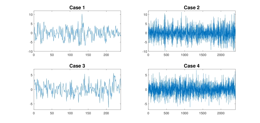
Figure 1: Sample trajectories of PAR model with Gaussian additive noise related to the cases considered in the simulation study.

For each of the cases, we simulate $M=1000$ trajectories of the given set-up. For each generated sample, we estimate the $\phi_{i}(v)$ parameters using all five considered methods (M1-M5). In such a way, we are able to obtain many realizations of all estimators which allow us to analyze their empirical distributions. As results, for each method and each estimated coefficient, we calculate the mean squared error (MSE) and, for selected cases, present also boxplots of obtained values. As some of the presented methods have hyperparameters needed to be preset, let us mention their values applied here. For methods M2, M3 and M4, we take here $s=p=2$ high-order Yule-Walker equations. Moreover, for the method M4 we set $\delta_{0}=0.001$ and $\delta=0.001$.

The MSE results in Case 1 for all considered methods are presented in Tab. 1. Most of all, one can clearly see the advantage of the proposed methods (M1-M4), which take the presence of the additive noise into account, above the classical Yule-Walker method (M5). In this case, the best results were obtained by the method M3. The boxplots of the estimated values for all considered methods in Case 1 are presented in Fig. 2. Most of all, one can see the difference between the results for the proposed methods and the method M5 in terms of the present bias – unlike the former, the latter seems to be significantly biased. In general, the level of this bias increases, the further the true value of the parameter is from zero.

Table 1: Parameter-wise and average mean squared errors obtained in Case 1 ($\phi_{2}(1)=-0.8$, $NT=240$) for all methods.

method	$\phi_{1}(1)$	$\phi_{1}(2)$	$\phi_{1}(3)$	$\phi_{2}(1)$	$\phi_{2}(2)$	$\phi_{2}(3)$	average
M1	0.0063	0.0188	0.0074	0.0091	0.0272	0.0030	0.0120
M2	0.0056	0.0169	0.0055	0.0091	0.0258	0.0029	0.0110
M3	0.0059	0.0168	0.0053	0.0081	0.0258	0.0027	0.0107
M4	0.0071	0.0184	0.0112	0.0158	0.0280	0.0053	0.0143
M5	0.0050	0.0795	0.0058	0.0114	0.1348	0.0046	0.0402

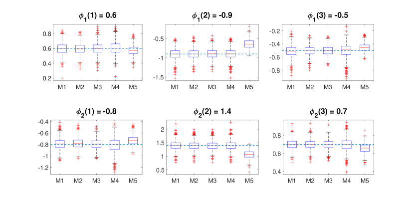
Figure 2: Boxplots of estimated values in Case 1 ($\phi_{2}(1)=-0.8$, $NT=240$) for all methods.

In Tab. 2, we present the MSE results obtained in Case 2. One can see that the performance of all methods improved in comparison to Case 1, which of course is expected as now the samples under consideration are much longer. However, for methods M1-M4 this change is much more significant, hence their advantage over classical Yule-Walker method is now relatively larger. Similar as for Case 1, method M3 yields the best results. For Case 2, let us also present the boxplots of estimated values in Fig. 3, where the similar behaviour as for Case 1 can be observed. Even for such long samples, the method M5 produces relatively large errors due to the presence of bias, which makes it worse than the proposed techniques.

Table 2: Parameter-wise and average mean squared errors obtained in Case 2 ($\phi_{2}(1)=-0.8$, $NT=2400$) for all methods.

method	$\phi_{1}(1)$	$\phi_{1}(2)$	$\phi_{1}(3)$	$\phi_{2}(1)$	$\phi_{2}(2)$	$\phi_{2}(3)$	average
M1	0.0006	0.0014	0.0006	0.0007	0.0019	0.0003	0.0009
M2	0.0005	0.0014	0.0005	0.0007	0.0019	0.0003	0.0009
M3	0.0005	0.0013	0.0005	0.0006	0.0019	0.0002	0.0008
M4	0.0008	0.0014	0.0012	0.0015	0.0019	0.0006	0.0012
M5	0.0009	0.0667	0.0025	0.0045	0.1108	0.0019	0.0312

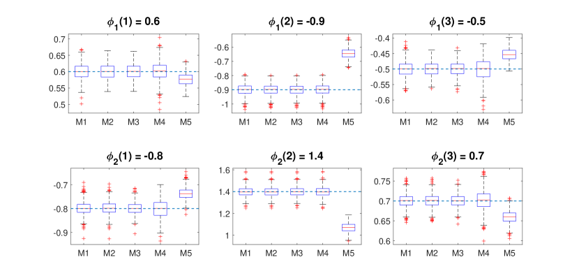
Figure 3: Boxplots of estimated values in Case 2 ($\phi_{2}(1)=-0.8$, $NT=2400$) for all methods.

The results for Case 3 are presented in Tab. 3. Let us remind that, in comparison to previous cases, we changed the value of $\phi_{2}(1)$ coefficient from -0.8 to -0.1, making it much closer to zero. Above all, let us note that method M1 clearly failed here, producing very significant errors for some parameters. This behaviour is caused by the fact that when the true coefficients values are close to zero, the matrix ${}_{p}\tilde{\mathbf{\Gamma}}^{Y}_{v}$ used in estimation with method M1 becomes close to singular. This issue is also discussed in [36], in the context of noise-corrupted autoregressive models. Hence, especially for a small amount of data, this approach might fail. In Case 4, where we consider longer samples, this drawback is slightly mitigated as can be seen in Tab. 4, but the method is still much less reliable than others. Another method with visible performance drop is method M4. In Case 3, its results are even worse than for method M5, but because of the previously mentioned improvement tendencies for longer samples, in Case 4 the method M4 gives again better results. However, in both setups, similarly as before, the best results are obtained by methods M2 and M3, in particular for the latter which can be clearly considered as the best approach in this simulation study.

Table 3: Parameter-wise and average mean squared errors obtained in Case 3 ($\phi_{2}(1)=-0.1$, $NT=240$) for all methods.

method	$\phi_{1}(1)$	$\phi_{1}(2)$	$\phi_{1}(3)$	$\phi_{2}(1)$	$\phi_{2}(2)$	$\phi_{2}(3)$	average
M1	0.0515	109.97	333.44	0.0210	51.2423	546.18	173.49
M2	0.0296	0.2278	0.0225	0.0139	0.1972	0.0466	0.0896
M3	0.0216	0.2008	0.0135	0.0125	0.1781	0.0270	0.0756
M4	0.0395	1.1913	0.0713	0.0215	0.8316	0.1365	0.3819
M5	0.0359	0.3895	0.0181	0.0090	0.4159	0.0557	0.1540

Table 4: Parameter-wise and average mean squared errors obtained in Case 4 ($\phi_{2}(1)=-0.1$, $NT=2400$) for all methods.

method	$\phi_{1}(1)$	$\phi_{1}(2)$	$\phi_{1}(3)$	$\phi_{2}(1)$	$\phi_{2}(2)$	$\phi_{2}(3)$	average
M1	0.0042	15.625	0.2566	0.0019	7.4705	0.3709	3.9549
M2	0.0038	0.0442	0.0043	0.0013	0.0373	0.0112	0.0170
M3	0.0023	0.0363	0.0017	0.0013	0.0314	0.0029	0.0127
M4	0.0037	0.1798	0.0066	0.0013	0.1582	0.0150	0.0608
M5	0.0248	0.3792	0.0138	0.0017	0.4056	0.0444	0.1449

5 Analysis of the simulated data – PAR model with additive outliers

To demonstrate the universality of the proposed estimation techniques, in this section we analyze two additional cases of the additive noise $\{Z_{t}\}$ in the model (1), namely when it is a sequence of additive outliers and when it is a mixture of the Gaussian additive noise and additive outliers. As it was mentioned in Section 1, especially the last case corresponds to real situations, where the measurements are disturbed by the additive errors (related to the noise of the device) and additional impulses that may be related to external sources.

In the presented simulation study, we consider the PAR model corresponding to Cases 1 and 2 described in Section 4. In order to avoid the comprehensive discussion of the influence of the level of the additive noise’s variance on the estimation results, we assume the variance of the additive noise considered in this part is on the same level as the variance of the Gaussian additive noise considered in the previous section ($\sigma_{Z}^{2}=0.8$). The analysis related to the sensitivity of the new estimation techniques to the variance of the additive noise is an essential issue and will be discussed in our future studies. In this part, we only analyze how the existence of additive outliers in the considered model influences the estimation. Similar as in Section 4 we provide the Monte Carlo simulations and in each case we simulate $M=1000$ trajectories corresponding to the considered cases. For each simulated trajectory, we estimate the parameters of the model, finally we calculate the mean squared errors and create the boxplots of the received estimators for selected cases. First, we analyze the case when the additive noise $\{Z_{t}\}$ in the model (1) is a sequence of additive outliers. More precisely, we assume that for each $t$, $\mathbb{P}(Z_{t}=10)=\mathbb{P}(Z_{t}=-10)=0.004$ and $\mathbb{P}(Z_{t}=0)=0.992$. In the further analysis the considered cases are called Case 1a and Case 2a, respectively, in order to highlight that they correspond to the Case 1 and Case 2, analyzed in the previous section. In Fig. 4 we demonstrate the exemplary trajectories of the considered model corresponding to Case 1a and Case 2a.

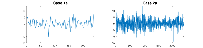
Figure 4: Sample trajectories of PAR model with additive outliers related to the Cases 1a and 2a considered in the simulation study.

The MSE results obtained for the Case 1a are presented in Tab. 5 and Fig. 5. Most of all, they confirm that the developed methods are able to handle also the cases where the additive outliers are present. In particular, once again they are much better than the method M5. However, one can see some changes of tendencies in comparison to the cases with Gaussian additive noise. In particular, the method M3, which yielded the best results in Section 4, here turned out to be less efficient than other introduced methods. The least average mean squared error was obtained for method M1.

Table 5: Parameter-wise and average mean squared errors obtained in Case 1a ($\phi_{2}(1)=-0.8$, $NT=240$) for all methods.

method	$\phi_{1}(1)$	$\phi_{1}(2)$	$\phi_{1}(3)$	$\phi_{2}(1)$	$\phi_{2}(2)$	$\phi_{2}(3)$	average
M1	0.0062	0.0158	0.0064	0.0086	0.0218	0.0029	0.0103
M2	0.0090	0.0189	0.0079	0.0153	0.0229	0.0032	0.0129
M3	0.0099	0.0257	0.0081	0.0204	0.0402	0.0044	0.0181
M4	0.0073	0.0161	0.0148	0.0256	0.0237	0.0058	0.0156
M5	0.0091	0.0828	0.0070	0.0165	0.1406	0.0057	0.0436

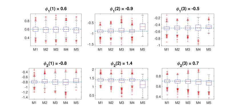
Figure 5: Boxplots of estimated values in Case 1a ($\phi_{2}(1)=-0.8$, $NT=240$) for all methods.

Next, let us analyze the Case 2a, where we consider longer samples. As can be seen in Tab. 6 and Fig. 6, the results indicate a higher efficiency than in the previous case, but the values obtained with the method M5 still exhibit its bias towards zero. Hence, similarly as before, for longer samples the advantage of proposed methods becomes even more significant. The best results, as in Case 1a, were obtained by method M1. However, one should be aware of the fact that for lower true values of $\phi_{i}(v)$ coefficients (see Cases 3 and 4 in Section 4) this method would still suffer from the mentioned causes.

Table 6: Parameter-wise and average mean squared errors obtained in Case 2a ($\phi_{2}(1)=-0.8$, $NT=2400$) for all methods.

method	$\phi_{1}(1)$	$\phi_{1}(2)$	$\phi_{1}(3)$	$\phi_{2}(1)$	$\phi_{2}(2)$	$\phi_{2}(3)$	average
M1	0.0005	0.0013	0.0005	0.0007	0.0019	0.0003	0.0009
M2	0.0013	0.0018	0.0009	0.0019	0.0019	0.0003	0.0013
M3	0.0011	0.0016	0.0010	0.0028	0.0020	0.0005	0.0015
M4	0.0010	0.0013	0.0040	0.0052	0.0020	0.0012	0.0024
M5	0.0015	0.0678	0.0025	0.0051	0.1127	0.0023	0.0320

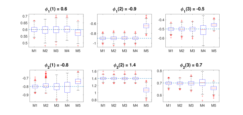
Figure 6: Boxplots of estimated values in Case 2a ($\phi_{2}(1)=-0.8$, $NT=2400$) for all methods.

As the second example of the model with additive outliers we consider the most extreme case, namely, when the additive noise $\{Z_{t}\}$ in Eq. (1) is a sequence of i.i.d. random variables being a sum of two independent sequences: Gaussian additive noise and additive outliers. More precisely, we assume that for each $t$

$$Z_{t}=Z_{t}^{(1)}+Z_{t}^{(2)},$$ (49)

where the sequences $\{Z_{t}^{(1)}\}$ and $\{Z_{t}^{(2)}\}$ are independent. Both of them constitute sequences of i.i.d. random variables. Moreover, for each $t$ the random variable $Z_{t}^{(1)}\sim N(0,0.2)$ and $Z_{t}^{(2)}$ is a discrete random variable such that $\mathbb{P}(Z_{t}^{(2)}=10)=\mathbb{P}(Z_{t}^{(2)}=-10)=0.003$ and $\mathbb{P}(Z_{t}^{(2)}=0)=0.994$. Taking such values of the parameters of both sequences’ distribution we ensure the same level of variance of the additive noise as it was considered in case of the Gaussian additive noise (see Section 4) and additive outliers discussed above. In the further analysis the cases considered in this part are called Case 1b and Case 2b in order to notice that they correspond to Case 1 and Case 2, respectively, considered in Section 4. In Fig. 7 we demonstrate the exemplary trajectories of the considered model corresponding to Case 1b and Case 2b.

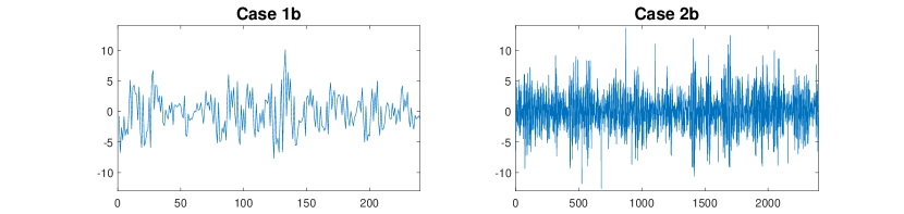
Figure 7: Sample trajectories of PAR model with Gaussian additive noise and additive outliers related to the Cases 1b and 2b considered in the simulation study.

The results for the Case 1b are given in Tab. 7 and illustrated in Fig. 8. Moreover, the results for the Case 2b are presented in Tab. 8 and Fig. 9. In general, the behaviour observed here can be described similarly as for Cases 1a and 2a. Once again, the advantage of proposed methods above the classical algorithm M5 is clear and becomes more visible for longer samples. In this part, just like in the previous one, the least average mean squared errors were obtained for method M1.

Table 7: Parameter-wise and average mean squared errors obtained in Case 1b ($\phi_{2}(1)=-0.8$, $NT=240$) for all methods.

method	$\phi_{1}(1)$	$\phi_{1}(2)$	$\phi_{1}(3)$	$\phi_{2}(1)$	$\phi_{2}(2)$	$\phi_{2}(3)$	average
M1	0.0060	0.0172	0.0064	0.0084	0.0222	0.0027	0.0105
M2	0.0077	0.0171	0.0070	0.0151	0.0216	0.0030	0.0119
M3	0.0090	0.0206	0.0081	0.0196	0.0328	0.0040	0.0157
M4	0.0073	0.0165	0.0144	0.0241	0.0241	0.0057	0.0154
M5	0.0077	0.0784	0.0066	0.0160	0.1295	0.0053	0.0406

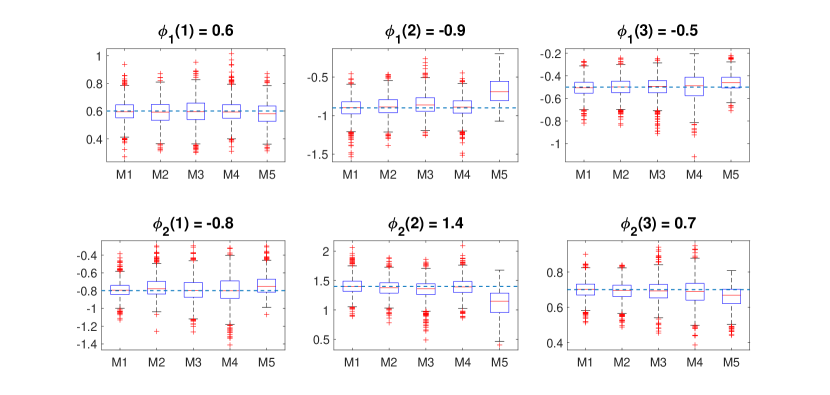
Figure 8: Boxplots of estimated values in Case 1b ($\phi_{2}(1)=-0.8$, $NT=240$) for all methods.

Table 8: Parameter-wise and average mean squared errors obtained in Case 2b ($\phi_{2}(1)=-0.8$, $NT=2400$) for all methods.

method	$\phi_{1}(1)$	$\phi_{1}(2)$	$\phi_{1}(3)$	$\phi_{2}(1)$	$\phi_{2}(2)$	$\phi_{2}(3)$	average
M1	0.0005	0.0014	0.0006	0.0008	0.0020	0.0003	0.0009
M2	0.0011	0.0016	0.0009	0.0018	0.0020	0.0003	0.0013
M3	0.0010	0.0015	0.0009	0.0024	0.0021	0.0004	0.0014
M4	0.0010	0.0014	0.0035	0.0048	0.0022	0.0011	0.0023
M5	0.0014	0.0656	0.0026	0.0052	0.1099	0.0020	0.0311

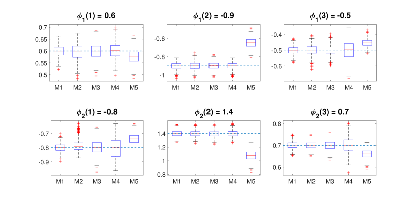
Figure 9: Boxplots of estimated values in Case 2b ($\phi_{2}(1)=-0.8$, $NT=2400$) for all methods.

6 Summary and discussion

In this paper, we have discussed the problem of identification and characterization of the general noise-corrupted PAR model. We assume here that innovations of PAR model and additive noise are finite-variance distributed. The main attention was paid to the estimation of the model parameters. We have proposed four Yule-Walker-based estimation techniques and demonstrated their efficiency for three additive noise types, namely, Gaussian distributed noise and two cases of non-Gaussian distributed noise (additive outliers, and the case when the disturbances are the sum of the Gaussian noise and additive outliers). The main motivation of the current research comes from the condition monitoring, where the models of real vibration might be used to develop an inverse filter to remove components related to mesh frequencies in gearbox vibrations. Analysis of the residual signal allows to detect local damage. Lack of precision during modelling results in distortions in residuals and poor damage detection efficiency. The presence of additive noise in the real vibration signals is very intuitive. Additionally, the existence of additive outliers in the signal is also often observed in practice and may significantly influence the estimation results. Thus, the introduction of estimation methods dedicated to the model with general additive disturbances may improve the efficiency of the techniques used for local damage detection. In the presented analysis, we have discussed only a few aspects of the considered problem, such as, e.g., the influence of the additive outliers on the estimation results, the sensitivity of the new techniques to the signal length and comparison of the efficiency of the proposed techniques in the considered cases. However, the presented results open new areas of interest that are crucial for signal processing techniques.

Funding

This work is supported by National Center of Science under Sheng2 project No. UMO-2021/40/Q/ST8/00024 ”NonGauMech - New methods of processing non-stationary signals (identification, segmentation, extraction, modeling) with non-Gaussian characteristics for the purpose of monitoring complex mechanical structures”.

Competing interests

The authors have no relevant financial or non-financial interests to disclose.

Data availability statement

The datasets generated and analysed during the current study are available from the corresponding author on reasonable request.

References

- [1] Jones R, Brelsford W. Time series with periodic structure. Biometrika. 1967;54(3-4):403–408.
- [2] Gardner W, editor. Cyclostationarity in communications and signal processing. New York: IEEE Press; 1994.
- [3] Bukofzer D. Optimum and suboptimum detector performance for signals in cyclostationary noise. IEEE J Ocean Eng. 1987;12:97–115.
- [4] Bloomfield P, Hurd HL, Lund RB. Periodic correlation in stratospheric ozone time series. J Time Ser Anal. 1994;15(2):127–150.
- [5] Dargaville R, Doney S, Fung I. Inter-annual variability in the interhemispheric atmospheric CO2 gradient. Tellus B. 2003;15:711–722.
- [6] Arora R, Sethares WA, Bucklew JA. Latent periodicities in genome sequences. IEEE J Sel Top Signal Process. 2008;2(3):332–342.
- [7] Gezici S. Theoretical limits for estimation of periodic movements in pulse-based UWB systems. IEEE J Sel Top Signal Process. 2007;1(3):405–417.
- [8] Antoni J, Bonnardot F, Raad A, et al. Cyclostationary modelling of rotating machine vibration signals. Mech Syst Signal Process. 2004;18(6):1285–1314.
- [9] Antoni J. Cyclic spectral analysis of rolling-element bearing signals: facts and fictions. J Sound Vib. 2007;304(3):497–529.
- [10] Wang D, Zhao X, Kou LL, et al. A simple and fast guideline for generating enhanced/squared envelope spectra from spectral coherence for bearing fault diagnosis. Mech Syst Signal Process. 2019;122:754–768.
- [11] Brockwell PJ, Davis RA. Introduction to time series and forecasting. New York: Springer; 2002.
- [12] Shin K, Feraday SA, Harris CJ, et al. Optimal autoregressive modelling of a measured noisy deterministic signal using singular-value decomposition. Mech Syst Signal Process. 2003;17(2):423–432.
- [13] Wyłomańska A, Obuchowski J, Zimroz R, et al. Periodic autoregressive modeling of vibration time series from planetary gearbox used in bucket wheel excavator. Cyclostationarity: Theory and Methods. 2014;:171–186.
- [14] Hallin M, Ingenbleek JF. Nonstationary Yule-Walker equations. Stat Probab Lett. 1983;1(4):189–195.
- [15] Lund R, Basawa IV. Recursive prediction and likelihood evaluation for periodic ARMA models. J Time Ser Anal. 2000;21(1):75–93.
- [16] Tesfaye YG, Meerschaert MM, Anderson PH. Identification of periodic autoregressive moving average models and their application to the modeling of river flows. Water Resour Res. 2006;42(1).
- [17] Grenier Y. Time-dependent ARMA modeling of nonstationary signals. IEEE Trans Acoust Speech Signal Process. 1983;31(4):899–911.
- [18] Hsiao T. Identification of time-varying autoregressive systems using maximum a posteriori estimation. IEEE Trans Signal Process. 2008;56(8):3497–3509.
- [19] Battaglia F, Cucina D, Rizzo M. Parsimonious periodic autoregressive models for time series with evolving trend and seasonality. Stat Comput. 2020;30:77–91.
- [20] Esfandiari M, Vorobyov SA, Karimi M. New estimation methods for autoregressive process in the presence of white observation noise. Signal Process. 2020;171:107480.
- [21] Diversi R, Guidorzi R, Soverini U. Identification of autoregressive models in the presence of additive noise. Int J Adapt Control Signal Process. 2008;22(5):465–481.
- [22] Mahmoudi A, Karimi M. Parameter estimation of autoregressive signals from observations corrupted with colored noise. Signal Process. 2010;90(1):157–164.
- [23] Çayır O, Ç Candan. Maximum likelihood autoregressive model parameter estimation with noise corrupted independent snapshots. Signal Process. 2021;186:108118.
- [24] Stoica P, Sorelius J. Subspace-based parameter estimation of symmetric noncausal autoregressive signals from noisy measurements. IEEE Trans Signal Process. 1999;47(2):321–331.
- [25] Mossberg M. High-accuracy instrumental variable identification of continuous-time autoregressive processes from irregularly sampled noisy data. IEEE Trans Signal Process. 2008;56(8):4087–4091.
- [26] Amanat A, Mahmoudi A, Hatam M. Two-dimensional noisy autoregressive estimation with application to joint frequency and direction of arrival estimation. Multidimens Syst Signal Process. 2018;29:671–685.
- [27] Sarnaglia AJQ, Reisen VA, Lévy-Leduc C. Robust estimation of periodic autoregressive processes in the presence of additive outliers. J Multivar Anal. 2010;101(9):2168–2183.
- [28] Sarnaglia AJQ, Reisen VA, Bondou P, et al. A robust estimation approach for fitting a PARMA model to real data. In: 2016 IEEE Statistical Signal Processing Workshop (SSP); 2016. p. 1–5.
- [29] Shao Q. Robust estimation for periodic autoregressive time series. J Time Ser Anal. 2008;29(2):251–263.
- [30] Bellini T. The forward search interactive outlier detection in cointegrated VAR analysis. Adv Data Anal Classif. 2016;10:351–373.
- [31] Cotta H, Reisen V, Bondon P, et al. Robust estimation of covariance and correlation functions of a stationary multivariate process. In: 25th European Signal Processing Conference (EUSIPCO 2017); 2017.
- [32] Wyłomańska A, Obuchowski J, Zimroz R, et al. Periodic autoregressive modeling of vibration time series from planetary gearbox used in bucket wheel excavator. Lect Notes Mech Eng. 2014;11:171–186.
- [33] Wyłomańska A, Obuchowski J, Zimroz R, et al. Influence of different signal characteristics to par model stability. Applied Condition Monitoring Cyclostationarity: Theory and Methods - II. 2015;:89–104.
- [34] Vecchia A. Periodic autoregressive-moving average (PARMA) modeling with applications to water resources. J Am Water Resour Assoc. 1985;21(5):721–730.
- [35] Żuławiński W, Wyłomańska A. New estimation method for periodic autoregressive time series of order 1 with additive noise. Int J Adv Eng Sci Appl Math. 2021;13:163–176.
- [36] Kay S. Noise compensation for autoregressive spectral estimates. IEEE Trans Acoust Speech Signal Process. 1980;28(3):292–303.