Morphology of the gas-rich debris disk around HD 121617 with SPHERE observations in polarized light

Abstract

Context. Debris disks are the signposts of collisionally eroding planetesimal circumstellar belts, whose study can put important constraints on the structure of extrasolar planetary systems. The best constraints on the morphology of disks are often obtained from spatially resolved observations in scattered light. Here, we investigate the young ($\sim$16 Myr) bright gas-rich debris disk around HD 121617.

Aims. We use new scattered-light observations with VLT/SPHERE to characterize the morphology and the dust properties of this disk. From these properties we can then derive constraints on the physical and dynamical environment of this system, for which significant amounts of gas have been detected.

Methods. The disk morphology is constrained by linear-polarimetric observations in the J band. Based on our modeling results and archival photometry, we also model the SED to put constraints on the total dust mass and the dust size distribution. We explore different scenarios that could explain these new constraints.

Results. We present the first resolved image in scattered light of the debris disk HD 121617. We fit the morphology of the disk, finding a semi-major axis of $78.3\pm 0.2$ au, an inclination of $43.1\pm 0.2^{\circ}$ and a position angle of the major axis with respect to north, of $239.8\pm 0.3^{\circ}$, compatible with the previous continuum and CO detection with ALMA. Our analysis shows that the disk has a very sharp inner edge, possibly sculpted by a yet-undetected planet or gas drag. While less sharp, its outer edge is steeper than expected for unperturbed disks, which could also be due to a planet or gas drag, but future observations probing the system farther from the main belt would help explore this further. The SED analysis leads to a dust mass of $0.21\pm 0.02\,M_{\oplus}$ and a minimum grain size of $0.87\pm 0.12\,$\text{\,}\mathrm{\SIUnitSymbolMicro m}$$, smaller than the blowout size by radiation pressure, which is not unexpected for very bright collisionally active disks.

1 Introduction

Debris disks are circumstellar disks orbiting $\gtrsim$ 10 Myr stars. They are detected around all types of stars of all ages (e.g. Wyatt et al. 2007; Sibthorpe et al. 2018) and are found around up to $\sim$ 75% of the stars in the youngest moving groups (e.g. the F stars in the $\beta$ Pic moving group, Pawellek et al. 2021). Debris disks are observed via $\leq 1$mm dust produced by destructive collisions between solid bodies up to $\sim$1-100s of km in size (Krivov & Wyatt 2021). Most of the disk’s mass is contained in the largest of these solid bodies which constitute planetesimal belts similar to the Kuiper belt objects (KBOs) in our Solar System. Those large bodies cannot be observed in extrasolar systems. However, the location of these belts can be probed in the mm (e.g. with ALMA), which targets the thermal emission of large mm-sized grains that are unaffected by stellar radiation pressure and thus have a dynamics similar to their larger parent bodies (e.g. Matrà et al. 2019). In contrast, scattered-light observations (e.g. at near-infrared wavelengths with SPHERE, Perrot et al. 2019) probe much smaller micron-sized dust, whose orbits are strongly affected by radiation pressure and whose location might strongly depart from that of the planetesimal belt (Thebault et al. 2014).

Detecting and spatially resolving debris disks in scattered light using the extreme adaptive optics high-contrast imagers (SPHERE, GPI, SCExAO Beuzit et al. 2019; Macintosh et al. 2014; Jovanovic et al. 2015) or space telescopes (e.g., HST Ford et al. 2003) has now become common (e.g. Esposito et al. 2020; Schneider et al. 2014; Feldt et al. 2017; Lagrange et al. 2016; Perrot et al. 2016). Linearly polarized light can also be observed with the Spectro Polarimetric High contrast Exoplanet REsearch (SPHERE) instrument, which provides an alternative and sensitive method to detect debris disks surrounding bright stars emitting unpolarized light (e.g. Engler et al. 2017; Olofsson et al. 2016; Arriaga et al. 2020, and others…). These polarimetric observations reach a contrast close to the photon-noise limit (van Holstein et al. 2021, appendix E) and the extracted disk parameters do not suffer from self-subtraction effects (Milli et al. 2012) as are seen with angular differential imaging (ADI, Marois et al. 2006) in total intensity. Polarized light provides additional information on the optical properties of dust compared to the total-intensity signal (e.g. Milli et al. 2019; Singh et al. 2021; Crotts et al. 2021). Thanks to the very high contrast and spatial resolution of SPHERE, remarkably sharp and deep images of debris disks can be obtained (e.g. Boccaletti et al. 2018; Olofsson et al. 2018), which provide information on the spatial distribution of dust that can be used to derive important information about the global structure of the planetary system (e.g. Lee & Chiang 2016). As an example, the detection of a sharp inner edge to the disk could be interpreted as the signature of a planet located close to the edge that has cleared all dust from its chaotic zone (e.g. Wisdom 1980; Quillen & Faber 2006; Lagrange et al. 2012).

Another potential mechanism that could shape the radial structure of a debris ring, with possible consequences on its inner and outer edges, is the drag due to gas, as it will selectively make small dust grains drift inward or outward depending on their sizes (Takeuchi & Artymowicz 2001; Olofsson et al. 2022a). These considerations are important because gas is now being detected in debris disks (e.g. Zuckerman & Song 2012; Hughes et al. 2018). In fact, mainly thanks to the Atacama Large Millimeter and Submillimeter Array (ALMA), it has recently been shown that the presence of gas in a young bright debris disk is the norm rather than the exception (Moór et al. 2017). The observed gas (mainly CO, carbon and oxygen) is thought to be released from volatiles contained initially in icy form in the planetesimals of these belts, providing access to the composition of the volatile phase of these KBO-like bodies (e.g. Zuckerman & Song 2012; Kral et al. 2016). In this scenario, both dust and gas would be of secondary origin. However, for the most massive gas disks, and only those, it is still possible that the observed gas is a relic of the protoplanetary disk phase that takes longer than expected to dissipate (e.g. Kóspál et al. 2013; Nakatani et al. 2021). Such a primordial origin is however not necessary because the presence of large amounts of CO can also be explained by gas released by planetesimals creating a layer of neutral carbon gas shielding CO from photodissociating (Kral et al. 2019). Some observational evidence seems to make the primordial origin less convincing than the secondary hypothesis (Hughes et al. 2017; Smirnov-Pinchukov et al. 2022). In systems with a significant amount of gas, interactions between gas and dust may become important and affect the dust size distribution at the smallest sizes, which may leave observable imprints (e.g. Bhowmik et al. 2019; Moór et al. 2019; Olofsson et al. 2022a).

In this paper, we study the debris disk around the young A1V star HD 121617, which is also surrounded by a massive gas disk (Moór et al. 2017). More precisely, this new study will present the first resolved scattered light observations of the debris disk around HD 121617, obtained at J band, in polarization with SPHERE. The debris disk has been known for about 25 years and has now been observed at a range of wavelengths from optical to mm (Mannings & Barlow 1998; Cutri & et al. 2012; Moór et al. 2017). Its fractional luminosity is close to $5\times 10^{-3}$ (Moór et al. 2011), which places it among the brightest disks observed to date. More information on the star and its disk is provided in section 2. In section 3, we present the new SPHERE observations of HD 121617. In section 4, we present the morphological analysis of the disk based on our resolved observations. In section 5, we present the spectral energy distribution (SED) analysis of the system, which allows us to recover information on the dust size distribution and total dust mass. Finally, in section 6, we discuss our results before concluding in section 7.

2 HD 121617

2.1 Stellar parameters

HD 121617 is an A1V (Houk 1978) main sequence star (Matrà et al. 2018), member of the Upper Centaurus Lupus (UCL) association (Hoogerwerf 2000; Gagné et al. 2018), with an age estimated to be $16$ $\pm$ 2 Myr, based on the age of the UCL association (Pecaut & Mamajek 2016). The distance of the star is $117.9$ $\pm$ 0.5 pc (DR3, Gaia Collaboration et al. 2016; Gaia collaboration et al. 2022). The most recent estimations of the stellar parameters are reported in different studies, for example in Rebollido et al. (2018) where the authors estimated the effective temperature $T_{\mathrm{eff}}=9285\,K$ and surface gravity of $\log\,g=4.45$. In Cotten & Song (2016), the effective temperature is estimated at $T_{eff}=8710\,K$ and a stellar radius at $R_{\star}=1.63\,R_{\odot}$, while Matrà et al. (2018) estimated the stellar luminosity at $L_{\star}=17.3\,L_{\odot}$ and the stellar mass at $M_{\star}=1.9\,M_{\odot}$. The galactic extinction is estimated by Gaia DR3 to $A_{0}=0.1331^{+0.0012}_{-0.0018}$ mag (Gaia Collaboration et al. 2016; Gaia collaboration et al. 2022) and the ratio between the extinction and the reddening to $R_{V}=3.25$ (Gontcharov & Mosenkov 2018).

2.2 Debris disk in the infrared

The presence of a disk around HD 121617 was first reported in Mannings & Barlow (1998) as an infrared excess at $12$, $25$, $60$ and $100\,$\text{\,}\mathrm{\SIUnitSymbolMicro m}$$ in the Infrared Astronomical Satellite (IRAS) Faint Source Survey Catalog (Moshir 1989). The first estimation of the temperature and radius of the disk was made by Fujiwara et al. (2013) using AKARI/IRC observations at $18\,$\text{\,}\mathrm{\SIUnitSymbolMicro m}$$ (Ishihara et al. 2010), on top of the previous Infrared Astronomical Satellite (IRAS) data as well as the Wide-field Infrared Survey Explorer (WISE) survey (Cutri & et al. 2012). Moór et al. (2011) reported a fractional luminosity of the disk $f_{\mathrm{disk}}=L_{\mathrm{disk}}/L_{\star}=4.8\times 10^{-3}$, based on the SED.

2.3 Gas and dust detection with ALMA

The first millimeter detection was reported in Moór et al. (2017) with ALMA at $1.3$ mm. They spatially resolved the disk in the continuum and detected spectrally resolved emission lines of several CO isotopologs, showing the presence of gas in the debris disk. The dust mass is estimated to be $1.4$ $\times$ $10^{-1}$ M_⊕ from the $1.3$ mm observations. They also constrained the morphology of the ring from the continuum observations (but not for the gas), with an inclination of $37$ $\pm$ $13^{\circ}$, a position angle of the major axis of $43$ $\pm$ $19^{\circ}$, a diameter of $152$ $\pm$ $15$ au, and a radial thickness of $52$ $\pm$ $17$ au, corresponding to the full width at half maximum (FWHM) of a the 2D-Gaussian used to model the ring (Moór et al. 2017). The ring size and thickness are corrected, according to the new distance of the star from Gaia DR3. As for the gas observations, using the standard isotopolog ratios of the local interstellar medium, they estimated a total ¹²CO mass of $1.8$ $\times$ $10^{-2}$ M_⊕, which makes it part of the most massive gas disks detected so far in debris disk systems, with a gas-to-dust ratio of $\sim$0.13.

3 Observations

3.1 SPHERE data

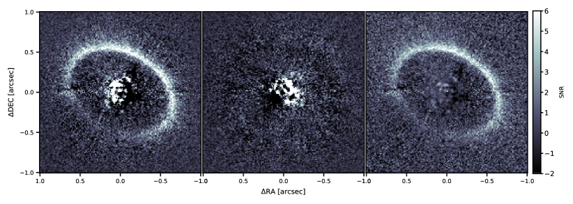
Figure 1: Left to right: $Q_{\phi}$ image, $U_{\phi}$ image, and S/N map of the $J$ band observations of HD 121617. North is up, east is left.

HD 121617 was observed with VLT/SPHERE (Beuzit et al. 2019) on the 28^th of April 2018 and the 20^th of May 2018 with the same configuration. Both epochs used the dual-beam polarimetric imaging (DPI, de Boer et al. 2020; van Holstein et al. 2020) mode of the Infra-Red Dual-band Imager and Spectrograph (IRDIS, Dohlen et al. 2008). The observations were done with the broadband J filter (BB_J, $\lambda_{c}$ = 1.245 $\text{\,}\mathrm{\SIUnitSymbolMicro m}$, $\Delta\lambda$ = 240 nm, de Boer et al. 2020), the N_ALC_YJH_S coronagraph mask, with an inner working angle of 185 mas (Boccaletti et al. 2008) and the pixel scale for this configuration is 12.26 mas per pixel (Maire et al. 2016). The observations were performed in field tracking mode and an offset angle was applied in the derotator to avoid the loss of polarisation as described in de Boer et al. (2020).

The DPI mode of IRDIS allows to construct the images of Stokes $Q$ and $U$. For this, the light is split into two parallel beams which pass two linear polarizers with orthogonal transmissions and are imaged simultaneously on the same detector, in the so-called Left and Right area. The subtraction of those images (Left minus Right) gives four different $Q^{\pm}$ and $U^{\pm}$ images, depending on the angle orientation of the half-wave plate (HWP). When the HWP switch angle is 0^∘, the $Q^{+}$ image is formed. HWP angles of 22.5^∘, 45^∘and 65.5^∘form respectively the images $U^{+}$, $Q^{-}$ and $U^{-}$. Finally, the Stokes $Q$ and $U$ images are constructed following:

$$X=\frac{1}{2}(X^{+}-X^{-})$$ (1)

where $X$ equals $U$ to reconstruct the Stokes $U$ vector and $X$ equals $Q$ to reconstruct the Stokes $Q$ vector. Thereby, a cycle of 4 HWP switch angles is necessary to obtain the Stokes $U$ and $Q$ vectors. More detailed explanations can be found in de Boer et al. (2020) and van Holstein et al. (2020). A total of $24$ HWP cycles were obtained (96 frames) for each epoch. The exposure time was set to $32$ seconds (DIT) for a trade-off between a maximum of time integration and avoiding saturation around the coronagraph, for a total integration time of $3072$ seconds (51.2 minutes) for each epoch. The observation sequence was performed following this order. First we acquired non-coronagraphic and non-saturated frames of the star (shifted out of the coronagraph by few hundreds mas, for the flux calibration. Then, the star is moved back behind the coronagraph to perform frame centering with the “waffle” mode, a sinusoidal pattern put on the deformable mirror in order to create 4 symmetric spots. The intersection of those 4 spots gives with a high accuracy the position of the star behind the coronagraph. The science acquisition is then obtained, with the polarimetric cycles described previously. At the end of the science sequence, another centering and flux calibration are performed in order to check the stability of the star centering and relative flux. Finally, a series of background calibration are performed by pointing the telescope away from the star. Both observations were taken with good atmospheric conditions with a seeing between $0.45$″and $0.75$″and a coherence time between $3$ ms and $8.5$ ms.

Data reduction was performed using the IRDIS Data reduction for Accurate Polarimetr (IRDAP) pipeline (van Holstein et al. 2020). The pipeline includes background and flat-field calibrations, star centering, correction for instrumental polarization and polarization crosstalk and the creation of the Stokes $Q$ and $U$ images. Then, IRDAP constructs the $Q_{\phi}$ and $U_{\phi}$ images (Schmid et al. 2006), which are used for further interpretation, following the definitions of de Boer et al. (2020):

$$\begin{split}Q_{\phi}=-Q\cos{2\Phi}-U\sin{2\Phi}\\ U_{\phi}=+Q\sin{2\Phi}-U\cos{2\Phi}\end{split}$$ (2)

where $\Phi$ is the position angle of the location of interest with respect to the stellar location. Figure 1 shows the final $Q_{\phi}$ and $U_{\phi}$ images obtained (the mean of the two epochs). The $Q_{\phi}$ image contains the polarimetric signal of the disk, revealing a bright and narrow ring. The ring shows a flux asymmetry between the North-West and the South-East sides. The $U_{\phi}$ image does not show any structured signal, expected for an optically thin disk (Canovas et al. 2015), and can therefore be used as a proxy for uncertainties in the modeling of the observations. Figure 1 (right) shows the derived signal-to-noise (S/N) map of $Q_{\phi}$. Several artifacts remain in the $Q_{\phi}$ and $U_{\phi}$ reduced images. In the East part of both images ($\Delta$RA = $0.5$″, $\Delta$DEC = $0$″) an horizontal artifact can be seen. This artifact, due to the SPHERE deformable mirror (fitting error, Cantalloube et al. 2019), is also present on the opposite side of the image, but less visible. Another artifact along the diagonal (from the top-right to the bottom-left) is present and is most likely due to the diffraction pattern of the VLT’s spiders, which were not aligned with the Lyot stop in field-tracking mode (low-order residuals, Cantalloube et al. 2019). Fortunately, the impact of those artifact is small due to the brightness of the disk and their locations.

3.2 Photometry

Using the VO SED Analyzer (VOSA) (Bayo et al. 2008) we gathered the photometric observations from different missions and instruments to build the SED of HD 121617. To determine the stellar parameters (section 2) we used the photometric measurements from TYCHO (B, V filters, Høg et al. 2000), Gaia (Gbp, G and Grp filters, Gaia Collaboration 2018), 2MASS (J, H and Ks filters, Cutri et al. 2003) and WISE (W1 and W2 filters, Wright et al. 2010). While WISE (W3 and W4 filters, Wright et al. 2010), Herschel/PACS (, $100\,$\text{\,}\mathrm{\SIUnitSymbolMicro m}$$ and $160\,$\text{\,}\mathrm{\SIUnitSymbolMicro m}$$, this work) and the 1.3 mm ALMA observations (Moór et al. 2017) are used to fit the infrared excess (section 5). We corrected the photometry to the extinction estimated by Gaia ($A_{V}=0.134$ mag, converted from $A_{0}$), assuming $R_{V}=3.25$ from Gontcharov & Mosenkov (2018). We converted $A_{V}$ to $A_{\lambda}$ for each filters using the extinction law from Cardelli et al. (1989, Eq. 1, 2 and 3) for wavelengths below $3.3\,$\text{\,}\mathrm{\SIUnitSymbolMicro m}$$ and the extinction law from Prato et al. (2003, $A_{\lambda}=(\frac{0.55}{\lambda[$\text{\,}\mathrm{\SIUnitSymbolMicro m}$]})^{1.6}\times A_{V}$) for wavelengths larger than $3.3$\text{\,}\mathrm{\SIUnitSymbolMicro m}$$. The photometric points, corrected and not corrected for extinction, are presented in Table LABEL:sedvalue.

The 100 $\text{\,}\mathrm{\SIUnitSymbolMicro m}$ PACS image is in fact marginally resolved; Figure 2 shows the data and a residual plot made by subtracting a point spread function (PSF) that was scaled to the image peak (where the PSF is an observation of the calibration star $\gamma$ Dra). Fitting the residual image with a disk model (as in Yelverton et al. 2019) finds disk parameters that are consistent with those found in section 4, but with significantly greater uncertainties, so we do not use this spatial information for any further analysis.

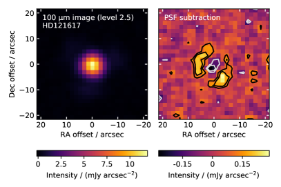
Figure 2: Left: Herschel/PACS observation of HD 121617 at 100 $\text{\,}\mathrm{\SIUnitSymbolMicro m}$. Right: Residual of the left image after a PSF subtraction performed with a calibration star. The continuum of the disk is marginally resolved.

Table 1: Photometric points for HD 121617.

Filter	Flux	Flux corr.	Error	$\lambda_{\rm eff}$	Ref.
-	[mJy]	[mJy]	[mJy]	[$\text{\,}\mathrm{\SIUnitSymbolMicro m}$]	-
TYCHO $B$	4372.0	5166.1	64.79	0.428	1
GAIA $Gbp$	3993.0	4577.1	37.59	0.504	2
TYCHO $V$	4499.0	5111.1	48.14	0.534	1
GAIA $G$	3957.0	4440.2	36.39	0.586	2
GAIA $Grp$	3236.0	3506.8	30.53	0.769	2
2MASS $J$	2067.0	2143.2	58.18	1.235	3
2MASS $H$	1400.0	1431.8	60.48	1.662	3
2MASS $Ks$	883.0	896.1	15.97	2.159	3
WISE $W1$	409.0	411.8	14.73	3.35	4
WISE $W2$	240.0	241.0	7.56	4.60	4
WISE $W3$	72.2	72.3	3.14	11.56	4
WISE $W4$	567.0	567.2	31.28	22.09	4
PACS 100	961.8	961.8	24.25	97.90	5
PACS 160	415.4	415.4	17.17	153.95	5
ALMA	1.86	1.86	0.29	1330.0	6

4 Morphological analysis of the SPHERE observations

4.1 Model and method

In order to constrain the disk morphology, we used the Debris DIsks Tool (DDiT, Olofsson et al. 2020) to create synthetic models of the debris disk in polarized intensity. DDiT was used with an Markov chain Monte Carlo (MCMC) code based on emcee (Foreman-Mackey et al. 2013) to determine the best values of the tested parameters. The geometry of the disk is defined by the inclination $i$ ($0^{\circ}$ for a face-on disk and $90^{\circ}$ for an edge-on disk) and the position angle of the major axis with respect to the north $\phi$. The dust density distribution of the disk is described in the radial $r$ and vertical $z$ directions as:

$$n(r,z)\propto\left[\left(\frac{r}{r_{0}}\right)^{-2\alpha_{\mathrm{in}}}+\left(\frac{r}{r_{0}}\right)^{-2\alpha_{\mathrm{out}}}\right]^{-1/2}\times e^{-z^{2}/2h^{2}}$$ (3)

with $n$ the dust grain volumetric density, $r_{0}$ the reference radius of the disk, $\alpha_{\mathrm{in}}$ and $\alpha_{\mathrm{out}}$ the inner and outer coefficients of the slope of the dust density distribution and $h$ the scale height of the disk. In the case of a non-eccentric circular debris disk, $r_{0}$ is a constant equal to the semi-major axis $a$. For an eccentric orbit, $r_{0}$ is defined as:

$$r_{0}(\gamma)=\frac{a(1-e^{2})}{1+e\cos{(\omega+\gamma)}}$$ (4)

with $e$ the eccentricity, $\omega$ the argument of the pericenter and $\gamma$ the azimuthal angle of the disk at $r_{0}$. Therefore, our fit will allow us to test whether the disk may be slightly eccentric. For the polarized scattering phase function we used the Henyey-Greenstein approximation (Henyey & Greenstein 1941), which is parameterized with the coefficient $g$ characterizing the scattering anisotropy of the dust (defined between $-1$, for backward scattering and $1$ for forward scattering) and the Rayleigh scattering function:

$$f_{HG}=\frac{1-\cos^{2}(\theta)}{1+\cos^{2}(\theta)}\frac{1}{4\pi}\frac{1-g^{2}}{(1+g^{2}-2g\cos{\theta})^{3/2}}$$ (5)

where $\theta$ is the scattering angle (Engler et al. 2017; Olofsson et al. 2019). Finally, the aspect ratio, $\psi=\arctan(h/r)$, is fixed to $0.05$ rad (Thébault 2009) due to the inclination of the disk, which is not adapted for a good estimation of $\psi$.

Priors for the 8 free parameters of the MCMC run ($a$, $i$, $\phi$, $g$, $\alpha_{\rm in}$, $\alpha_{\rm out}$, $e$, $\omega$) are presented in Table LABEL:mcmcparam. To compare each model to the data and determine the best value of the free parameters we proceed as follows. For each iteration of the MCMC run, the model is first convolved by a 2D normal distribution with a standard deviation of $2$ pixels (corresponding to the full width at half maximum of the off-axis image, to avoid an additional source of noise). Then the flux of the model is scaled to best match the data and the scaling factor $S_{\mathrm{scale}}$ is estimated as:

$$S_{\mathrm{scale}}=\frac{\sum\frac{I_{\mathrm{data}}\times I_{\mathrm{model}}}{\sigma^{2}}}{\sum\left(\frac{I_{\mathrm{model}}}{\sigma}\right)^{2}}$$ (6)

with $I_{\mathrm{data}}$ the 2-dimensional $Q_{\phi}$ image of the disk, $I_{\mathrm{model}}$ the 2-dimensional synthetic $Q_{\phi}$ image of the disk and $\sigma$ the noise map. This scaling is performed since DDiT produces images with no absolute flux for the reason that the latter depends on the total dust mass. The minimization is performed in an area including the disk and excluding the central part of the image where the residual star light remains. We selected the area between 0.25″ and 1.1″ from the star position (respectively, 29 and 129 au in projected separation). In that way, we do not exclude the potential extended signal of the disk in the outer part. In this area, the $\chi^{2}$ is computed following:

$$\chi^{2}=\left(\frac{I_{\mathrm{data}}-S_{\mathrm{scale}}\times I_{\mathrm{model}}}{\sigma}\right)^{2}$$ (7)

Finally, this $\chi^{2}$ is provided as the log likelihood to the MCMC for the optimization of the free parameters. The MCMC is run with 80 walkers with a length of 500 and a burn-in fixed at 100 steps.

4.2 Noise map and uncertainties

The noise map $\sigma$ is given by the $U_{\phi}$ image, which contain the same noise that the $Q_{\phi}$ image, without the astrophysical signal. To build the noise map, we compute the standard deviation per pixel in a small ring centered to the star. To take account for the correlation between pixels we add to the standard deviation an inflation term as described in Hinkley et al. (2021). This inflation term considers the spatial correlation of the PSF through the instrumental FWHM (40 mas or 3.3 pixels) and the radial elongation of the speckles due to the filter’s bandwidth. Therefore the noise map is computed as:

$$\sigma(r)=\sqrt{FWHM\times r\times\frac{\Delta\lambda}{\lambda_{c}}}\times\sigma_{std}(r)$$ (8)

with $r$ the angular separation, FWMH = 3.3 pixels, $\Delta\lambda$ the filter’s bandwidth, $\lambda_{c}$ the central wavelength of the filter and $\sigma_{std}(r)$ the radial standard deviation per pixel of the $U_{\phi}$ image. This is a conservative method which increases the uncertainties from the MCMC, which are usually under-estimated. In addition, Langlois et al. (2021) gives the typical error on the star center for the SpHere INfrared survey for Exoplanets (SHINE), which is 1.5 mas ($\sim$0.18 au).

4.3 Results of the MCMC analysis

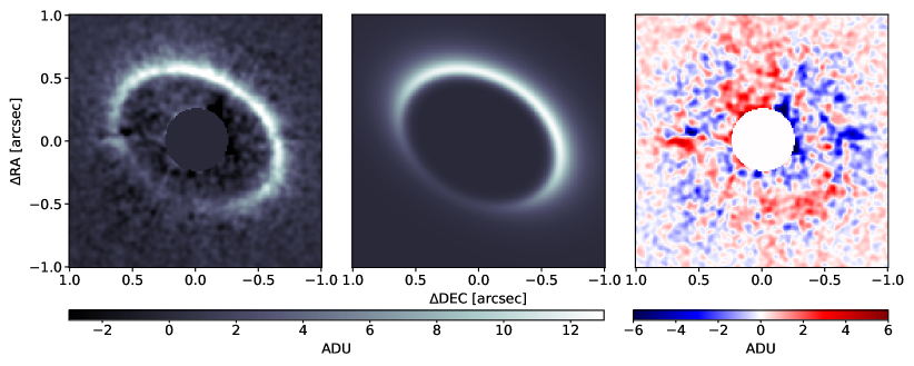
Figure 3: From left to right: The $Q_{\phi}$ image, the best model and the residual image after the subtraction of the best model from the $Q_{\phi}$ image. The grey area in the middle of each image is a numerical mask to exclude the residual star light.

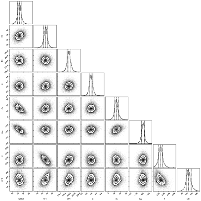
Figure 8: Corner-plot for the MCMC analysis. From left to right and top to bot: $a$ ($r_{0}$), $i$, $\phi$, $g$, $\alpha_{\mathrm{in}}$, $\alpha_{\mathrm{out}}$, $e$ and $\omega$. Middle dash-lines are the more probable value and external dash-lines are the 1-$\sigma$ error.

The results of the MCMC analysis are summarized in Table LABEL:mcmcparam. The best fit values are derived from the corner plots of the MCMC analysis, and their error bars are 1-$\sigma$ of the corresponding probability density function (PDF) for each given parameter (Fig. 8). Figure 3 shows the data (left), the best model (middle) and the residual image (right). Since most of the signal from the disk is accounted for and therefore not visible on the residuals, our best-fit model can explain the observations.

Table 2: Priors and results of MCMC analysis.

Parameters	Priors	Best-fit
		value
$a$ [au]	[75 ; 95]	78.6 $\pm$ 0.6
$i$ [∘]	[30 ; 60]	43.4 $\pm$ 0.8
$\phi$ [∘]	[220 ; 260]	240.0 $\pm$ 0.9
$g$	[0 ; 0.9]	0.60 $\pm$0.04
$\alpha_{\mathrm{in}}$	[2 ; 35]	18.9 $\pm$ 2.3
$\alpha_{\mathrm{out}}$	[-15 ; -2]	-5.8 $\pm$ 0.4
$e$	[0, 0.1]	0.03 $\pm$ 0.01
$\omega$ [∘]	[60 ; 200]	131.0 $\pm$ 15.1

We improve the constraints on the geometry of the disk compared to previous ALMA study (Moór et al. 2017). The inner edge of the disk observed with SPHERE is far enough from the star not to be affected by artifacts of residual light. Moreover, we use polarimetric observations, which do not necessitate post-processing techniques such as ADI and the results do not suffer from, for example, self-subtraction effects as can be the case for total intensity images. The SPHERE and ALMA results are compatible as we find a semi-major axis of $78.6$ $\pm$ $0.6$ au (vs. $76$ $\pm$ $8$ au), an inclination of $43.4$ $\pm$ $0.7^{\circ}$ (vs. $37$ $\pm$ $13^{\circ}$) and a position angle of the major axis of $240.0$ $\pm$ $0.9^{\circ}$ (vs. $223$ $\pm$ $19^{\circ}$). However the ring observed with SPHERE is much narrower compared to that observed with ALMA. The equivalent full width at half maximum (FWHM) of the disk in the SPHERE image is around 23 au (0.2″), while Moór et al. (2017) reported a FWHM of $52\pm 17$ au (0.44″). The difference can be explained by the larger angular beam size of the ALMA observations ($\sim$ 0.5″) so that the mm-dust ring is not resolved. In contrast, in the SPHERE observations the angular resolution of 0.03″allows us to resolve the ring’s width.

We find that the shape of the dust density distribution for the inner edge of the ring is extremely steep, with a power-law slope $\alpha_{\mathrm{in}}$ = $18.9$ $\pm$ $2.3$. The outer edge of the ring is also steeper than the expected dust density distribution for an evolved debris disk (Thébault & Wu 2008) with a power law of slope $\alpha_{\mathrm{out}}$ = $-5.8$ $\pm$ $0.4$ instead of the typical $\alpha_{\mathrm{out}}$ = $-1.5$. In Figure 4, we show the radial profiles along the major axis for the North-East and South-West directions, compared to the radial profile of the best model and the $1\sigma$ noise level from the $U_{\phi}$ image. Radial profiles are obtained by averaging a band of 6 pixels width along the major axis.

Finally, our analysis also shows that the disk is slightly eccentric, with an eccentricity of $0.03$ $\pm$ $0.01$. With a semi-major axis of $78.6$ $\pm$ $0.6$ au, this leads to an apocenter at $81.0$ $\pm$ $1.4$ au and a pericenter at $76.2$ $\pm$ $1.4$ au from the star, with the argument of the pericenter being at $131.0$ $\pm$ $15.1^{\circ}$.

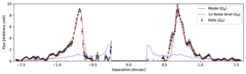
Figure 4: $Q_{\phi}$ radial profile following the projected major axis (6 pixels width) from the South-West to the North-East of the disk with the corresponding error bars (black points). The radial profile of the best model (red dashed line) and the Noise level obtained with the azimuthal standard deviation of the $U_{\phi}$ image (blue dotted line).

5 SED modeling

The analysis made with DDiT was focusing on the disk morphology. In this section we use those previously constrained parameters to estimate the dust properties. This is indeed a good way to proceed because SED fitting is a degenerate problem where the radial distance of the belt and the minimum grain size are correlated with each other. But once the belt location is fixed, we can directly constrain the grain properties.

5.1 SED with MCFOST

MCFOST (Pinte et al. 2006, 2009) is a 3 dimensional radiative transfer code for circumstellar disks, which can produce synthetic SED, images or absorption lines for specific systems. The code was initially developed for protoplanetary disks (optically thick, with gas, in local thermal equilibrium or not), but is also suitable for optically thin debris disks. We used MCFOST to compute the SED of HD 121617 with the aim of constraining the following dust parameters: the dust mass M_dust, the minimum grain size radius s_min, and the power law of the grain size distribution $q$. In MCFOST, stellar parameters are defined by the the Kurucz model (Castelli & Kurucz 2003) which corresponds the most to the SED. The selected model is the Kurucz model at T${}_{\rm eff}=9500$ K, log $g=5.0$ and the assuming the solar metallicity. The procedure to determined this model is presented in Appendix A. The disk morphology is defined by the results of the MCMC analysis of Section 4 (though we assumed a disk with zero eccentricity) with $a=78.6$ au, $i=43.4^{\circ}$, $\phi=240.0^{\circ}$, $\alpha_{\mathrm{out}}=-5.8$, and $\alpha_{\mathrm{in}}=18.9$. For the sake of simplicity and given the small eccentricity ($\sim 0.03$) we fix the eccentricity to zero. For the grain properties, we used the Mie theory (i.e., compact spherical grains), with a maximum grain size radius s${}_{\mathrm{max}}=1000\,$\text{\,}\mathrm{\SIUnitSymbolMicro m}$$ and we used the optical constant of astrosilicate grains (Draine & Lee 1984). Several studies of HR 4796 shows that Mie theory is not always adapted to described the dust grains geometry (Perrin et al. 2015; Milli et al. 2019). However, the measurement of the scattering phase function of a total intensity observation in required to constrain the dust grains geometry, in addition of the scattering phase function in polarimetry. Unfortunately the total intensity is not available for HD 121617, yet.

Then MCFOST is used to produce a synthetic SED of the system with a log-spaced sampling of 300 wavelengths from $0.1\,$\text{\,}\mathrm{\SIUnitSymbolMicro m}$$ to $1500\,$\text{\,}\mathrm{\SIUnitSymbolMicro m}$$. This synthetic SED is finally converted into synthetic photometric points for specific filters for comparison with photometric data. We proceeded using MCFOST in the non-LTE configuration. Since the disk should be optically thin, the infrared flux scales linearly with the total dust mass. Therefore, we fixed the dust mass and afterwards find the scaling factor $S_{\mathrm{flux}}$ that minimizes the residuals. A posteriori, we checked that the best fit solution indeed remains in the optically thin regime at all wavelengths with $\tau$ = 0.19 at $1,245\,$\text{\,}\mathrm{\SIUnitSymbolMicro m}$$ in the mid plane. The scaling factor $S_{\mathrm{flux}}$ is computed as:

$$S_{flux}=\frac{\sum\limits_{\lambda}\frac{F_{disk}(\lambda)}{\sigma(\lambda)^{2}}[F_{obs}(\lambda)-F_{star}(\lambda)]}{\sum\limits_{\lambda}\frac{F_{disk}(\lambda)^{2}}{\sigma(\lambda)^{2}}},$$ (9)

where $F_{\mathrm{obs}}(\lambda)$ is the observed flux for the $\lambda$ filter, $\sigma(\lambda)$ the observed flux error for the $\lambda$ filter. $F_{\mathrm{disk}}(\lambda)$ and $F_{\mathrm{star}}(\lambda)$ are, respectively, the synthetic flux of the disk component and the star component for the $\lambda$ filter from MCFOST.

To determine the best values of s_min and $q$, they are sampled into a grid of values (Tab. LABEL:mcfostparam). The $\chi^{2}$ is computed with the infrared photometry in the same way as for the star parameters analysis in section 2, including the following filters: WISE $W3$, WISE $W4$, PACS 100, PACS 160 and the ALMA observation at 1.33 mm. We did not consider filters below $10\,$\text{\,}\mathrm{\SIUnitSymbolMicro m}$$ because the disk contribution at those wavelengths is negligible compared to that of the star.

5.2 Results

Table LABEL:mcfostparam shows the results of the analysis with MCFOST, with values for the best-fit model derived from the PDFs shown in Fig. 5. The central value is taken to be when the cumulated PDF reaches 50% of the maximum while the error bars are for 16% and 84%, respectively. We find $s_{\mathrm{min}}\,=\,0.87^{+0.12}_{-0.13}\,$\text{\,}\mathrm{\SIUnitSymbolMicro m}$$, $q\,=\,-3.53$ $\pm$ $0.05$ and $M_{\mathrm{dust}}\,=\,0.21\pm 0.02\,M_{\oplus}$. As the dust mass is fixed via a scaling to the SED, we cannot directly compute the PDF for the mass. Instead, we randomly sample the output distribution of $M_{\mathrm{dust}}$ to produce a homogeneous grid of values, suitable to produce a PDF. This operation is repeated 1000 times for averaging purposes. These results are discussed in the next section.

Table 3: Parameters and results of the MCFOST analysis.

Parameter	Interval	Step	Best-fit model
$s_{\mathrm{min}}$ [$\text{\,}\mathrm{\SIUnitSymbolMicro m}$]	[0.30, 1.10]	0.05	$0.87^{+0.12}_{-0.13}$
$q$	[-3.8, -3.35]	0.05	$-3.53$ $\pm$ $0.05$
Mdust [M⊕]	[0.27]	– a	$0.21$ $\pm$ $0.02$

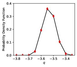
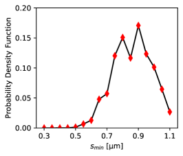
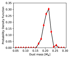
Figure 5: Probability Density Function (PDF) for $q$, $s_{\mathrm{min}}$ and M_dust.

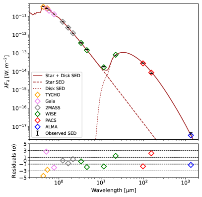
Figure 6: SED of the HD 121617 system (top) and the residuals after subtraction of the best-fit model (bottom). The best model of the star is represented by the brown dashed line and that of the disk by the brown dotted line, while their sum is the brown solid line. The photometric points are represented with vertical black symbols including error bars and the instrument used for the observations are shown with diamonds of different colors.

6 Discussion

6.1 Radial profile

Our results lead to a high value of $\alpha_{\mathrm{in}}=18.9$, corresponding to a very sharp inner edge of the disk. Such sharp inner edges have been witnessed around several other systems (see Table E.1 in Adam et al. 2021), and would indicate that ”something” is shaping them, the most likely explanation being that a sharp inner edge corresponds to the outer limit of the chaotic region surrounding a yet-undetected planet just located inward of the belt (e.g. Lagrange et al. 2012). Note that, contrary to outer edges, radiation pressure or stellar wind do not place small grains in the dynamically ”forbidden” region inward of the inner edge, which probably explains why sharp inner edges are more commonly observed than sharp outer ones (Adam et al. 2021). Poynting-Robertson drag could make small grains spiral inward, which could smooth out the sharpness of an inner disk edge, but the fraction of grains that can escape the main belt this way should be negligible for a very bright and collisionally-active disk such as HD 121617 (Wyatt 2005).

For the outer edge of the disk radial profile, we get $\alpha_{\mathrm{out}}=-5.8$, corresponding to a slope for the radial surface density profile in $-4.8$. This is more than the canonical slope in $-1.5$ (or in $-3.5$ for the flux) that is expected in the outer regions beyond a collision-dominated belt of parent bodies, under the competing effect of collisional activity within the belt and radiation pressure (or stellar wind) placing small grains on highly eccentric orbits outside of it (Strubbe & Chiang 2006; Thébault & Wu 2008). Note, however, that this $-1.5$ slope is not supposed to be reached immediately beyond the main belt, but after a transition region, of relative width $\Delta r/r_{0}\sim 0.2-0.3$, where the radial profile can be significantly steeper (Thebault et al. 2012, 2014). In the present case, the radial profile is constrained out to $1.1$″, after which the noise begins to dominate the signal (Fig. 4), which is approximately $40\%$ outside of the peak radial location. This is slightly more than the theoretical width of the ”natural” transition region beyond a collisional belt and could thus be interpreted as the signature of some additional removal process, such as dynamical perturbations by a planet or a stellar companion (Thébault 2012; Lagrange et al. 2012). Another possible explanation for a sharp density drop beyond a belt of parent bodies could be that the belt is dynamically ”cold”, with a low collisional activity that creates a dearth of small grains with respect to larger ones (Thébault & Wu 2008). However, this scenario appears unlikely in the present case, given the very high fractional luminosity ($\sim 4.8\times 10^{-3}$) of this disk, which should indicate a high level of dustiness.

At any rate, our understanding of both the inner and outer edges would greatly benefit from future observations constraining the disk’s radial profile further away from the main belt and also the potential presence of planets just inside or outside of it (e.g. with the Webb Space Telescope).

6.2 Dust mass

In debris disks the bulk of the mass is carried by large bodies that we cannot see neither with the full SED nor in the submm. However, we have access to the dust mass via mm-observations.

The value of $M_{\mathrm{dust}}=0.21\,M_{\oplus}$ we find is slightly higher than the dust mass obtained by Moór et al. (2017) from the flux density at 1.3mm, $0.12\,M_{\oplus}$. The difference between the two values is likely to be due to the fact that we use the whole SED to compute the mass whereas it is only based on the $1.3$ mm flux in the other study. Moreover, we use slightly different assumptions for the dust composition and opacities, which can lead to this kind of differences. However, these differences are relatively limited and our $M_{\mathrm{dust}}$ value remains compatible with previous estimates.

6.3 Size distribution and smallest grains

The best-fit value found for $q$, the power law of the grain size distribution, is $-3.53$, which is remarkably close to the canonical value $-3.5$ expected for infinite self-similar collisional cascades at steady-state (Dohnanyi 1969), and is fully compatible with size distribution profiles found in more realistic numerical explorations of collisional debris disks (Thébault & Augereau 2007; Kral et al. 2013).

As for the minimum grain size $s_{\mathrm{min}}=0.87\,$\text{\,}\mathrm{\SIUnitSymbolMicro m}$$ that we find, it is useful to compare it to the blowout size $s_{\mathrm{blow}}$ corresponding to the grain size for which the ratio $\beta$ between the radiation pressure ($F_{\mathrm{rad}}$) and the gravitation force ($F_{\mathrm{grav}}$) is equal to 0.5. Grains smaller than $s_{\mathrm{blow}}$ that are produced from parent bodies on circular orbits are ejected out of the system due to radiation pressure. $\beta$ is defined by:

$$\beta=0.5738Q_{\mathrm{pr}}\left(\frac{1\,{\rm g\,cm}^{-3}}{\rho_{\mathrm{d}}}\right)\left(\frac{1\,$\text{\,}\mathrm{\SIUnitSymbolMicro m}$}{s}\right)\frac{L/L_{\odot}}{M/M_{\odot}},$$ (10)

where $L$ is the stellar luminosity, $G$ the gravitational constant, $M$ the stellar mass, $c$ the speed of light, $Q_{\mathrm{pr}}$ the radiation pressure efficiency averaged over the stellar spectrum, and $\rho_{\mathrm{d}}$ the dust density. We assume $Q_{\mathrm{pr}}=1$ for geometric optics approximation and $\rho_{\mathrm{d}}=3.3\,{\rm g.cm}^{-3}$ for typical astrosilicate grains (Krivov et al. 2009). With the stellar parameters from Appendix A, we obtain $s_{\mathrm{blow}}=2.91\,$\text{\,}\mathrm{\SIUnitSymbolMicro m}$$, which is $\sim 3$ times larger than $s_{\mathrm{min}}$.

We cannot rule out that this difference is due to assumptions made about the grain geometry, such as $Q_{\mathrm{pr}}=1$, or chemical composition (pure astrosilicates). Pawellek & Krivov (2015) show indeed that those parameters can have an important contribution to the blowout size. In particular, for astrosilicate the value of $Q_{\mathrm{pr}}$ varies between 2 and 0.2 as function of the wavelength (Pawellek & Krivov 2015, Fig. 2). However, other dust compositions (such as carbon, ice or a mix) have lower dust densities, implying a higher blowout size.

If, however, this discrepancy between $s_{\mathrm{blow}}$ and $s_{\mathrm{min}}$ is real, then HD 121617 would join the handful of systems, such as HD 32297, AU Mic, HD 15115 or HD 61005 (Thebault & Kral 2019), for which a significant presence of grains with $\beta>0.5$ has been inferred. Such a presence has often been interpreted as due to violent and/or transient events, such as the catastrophic breakup of a large planetesimal (Johnson et al. 2012; Kral et al. 2015) or a so-called collisional avalanche (Grigorieva et al. 2007; Thebault & Kral 2018), with the caveat that such events might be short lived and statistically unlikely. However, the numerical exploration of Thebault & Kral (2019) has shown that, for bright disks around A stars, there is a significant population of $s<s_{\mathrm{blow}}$ grains even for a ”standard” debris disk at collisional steady-state. HD 121617, with a $f_{\mathrm{d}}=4.8\times 10^{-3}$ disk around an A1V central star, would nicely fit into this category.

Another possible explanation for the presence of small $\beta>0.5$ particles could be the effect of the gas that has been unambiguously detected in this system. Gas drag could indeed slow down the outward motion of unbound grains (Bhowmik et al. 2019) and push small micron-sized bound grains in regions where collisional activity is lower and lifetimes are longer (Olofsson et al. 2022b). This potential effect of gas on the observed dust, which could also affect the profile of the belt’s inner and outer edges, is discussed in more detail in the next subsection.

6.4 Effect of gas on the dust grains

The results we have obtained so far do not necessarily require the presence of gas to be explained, but we note that large amounts of CO ($\sim 2\times 10^{-2}$ M_⊕) are present in the system (Moór et al. 2017), which may lead to the gas dragging the smallest dust grains (Takeuchi & Artymowicz 2001). To verify this, we calculate the stopping time of grains of size $s$, of bulk density $\rho_{\mathrm{d}}$, located in a disk at 78 au of radial extent $\Delta R$, bathed in a total mass of gas $M_{\rm gas}$, which leads to

$$T_{\mathrm{s}}\sim 6\,\left(\frac{\rho_{\mathrm{d}}}{2\,{\rm g/cm}^{3}}\right)\left(\frac{s}{1\,$\text{\,}\mathrm{\SIUnitSymbolMicro m}$}\right)\left(\frac{M_{\rm gas}}{2\times 10^{-2}\,{\rm M}_{\oplus}}\right)^{-1}\left(\frac{\Delta R}{50\,{\rm au}}\right).$$ (11)

A particle with a stopping time close to 1 orbital period will react to gas in about one dynamical timescale (the dust grain is said to be marginally coupled). Therefore, we find that the smallest grains in the system ($\sim$ 1 $\text{\,}\mathrm{\SIUnitSymbolMicro m}$) can begin to respond to the presence of gas within tens of orbital timescales considering only CO is present. In the presence of radiation pressure, these grains are expected to move slowly outward (e.g. Takeuchi & Artymowicz 2001). The final parking location of these grains is where $\beta=\eta$, where $\eta$ is related to the gas pressure gradient and sets the gas velocity to $v_{\mathrm{k}}\sqrt{1-\eta}$ ($v_{\mathrm{k}}$ being the Keplerian velocity). However, they can be destroyed by collisions faster than they reach this parking location, depending on the mass of gas and the density of the dust disk (Olofsson et al. 2022a). Overall, the surface brightness radial slope is expected to be shallower than usual (i.e. closer to -2 than -3.5) beyond the disk, in the halo. Before reaching this halo-like slope, there is an abrupt transition where the planetesimal belt stops, leading to surface brightness slopes $<-5$ over short radial distances. However, the latter is true even in the case where no gas is present (Thébault & Augereau 2007). Although the abrupt transition can be observed with SPHERE, the halo is diluted in the noise and its radial slope cannot be calculated from current observations. The main conclusion is that, even though gas is expected to be able to drag the smallest grains, its effects are not detectable on the radial profiles given current observations.

It is expected that CO will photodissociate and create some carbon and oxygen. Depending on the amount of shielding and the viscosity of the gas disk, the number densities of carbon and oxygen may exceed that of CO (e.g. Kral et al. 2019). In the case where there is much more mass than $\sim 2\times 10^{-2}$ M_⊕ (e.g. carbon and oxygen dominate), we still expect the same general conclusion on the radial profile (even if H₂ dominates, i.e. primordial origin). The main difference will be that small grains will move outward more quickly and have a better chance of reaching their parking place before being destroyed by collisions.

However, one major difference is in the vertical profile of the grains. In the case of low gas masses where CO dominates the gas mass, vertical settling should only be significant for the smallest grains observed in scattered light, but it is difficult to spot in such an inclined system (Olofsson et al. 2022a). For more massive gas disks, the larger grains will have time to settle, creating needle-like disks in the sub-mm as well (Olofsson et al. 2022a). This difference would be easier to spot for an edge-on system but is difficult given the geometry of the disk around HD 121617.

Finally, one may wonder whether the steep inner edge may be explained by the presence of gas. As explained in section 6.1, many disks observed in scattered light have steep inner edges without gas being detected, and other causes such as the presence of a planet (see section 6.1) provide a good explanation for their origins. However, we note that the gas helps to carve this steep inner edge as the smallest micron-sized grains observed in scattered light would be pushed outward on $\sim$ 10 dynamical timescales (see Eq. 11), which is to be compared to the timescale for refilling them, a collisional timescale. For the smallest grains, the collision timescale can be approximated by $(\tau\Omega)^{-1}$, which corresponds to 200 dynamical timescales, given the optical depth $\tau\sim 5\times 10^{-3}$. The order of magnitude difference between the two timescales means that the smallest micron-sized grains would be slightly depleted in the innermost region, which cannot be refilled by grains coming from closer in regions. Finer observations and numerical simulations dealing with both dynamics and collisions in the presence of gas would be needed to draw more solid conclusions as to whether gas drag can really create steeper inner edges.

7 Conclusion

Using the polarimetric mode of the VLT/SPHERE-IRDIS instrument, we have resolved the gas-rich debris disk around the star HD 121617 for the first time in scattered light. The observations were made in 2018 using the dual-beam polarimetric imaging (DPI) mode in J band with a corresponding angular resolution of 0.03″  (or $\sim 3.5$ au), an order of magnitude better than previous ALMA observations in the mm (Moór et al. 2017).

The high contrast of the images coupled with the high angular resolution allows us to significantly improve the previous constraints on the disk morphology. We fit the image using a disk located at a semi-major axis $a$, with an inclination $i$ and an eccentricity $e$ with a density made up of two power laws $\alpha_{\rm in}$ and $\alpha_{\rm out}$. Using the radiative transfer code DDiT in an MCMC fashion, we find that the best fit is $a=78.6\pm 0.6$ au, $i=43.4\pm 0.8^{\circ}$, $e=0.03\pm 0.01$, $\alpha_{\rm in}=18.9\pm 2.3$ and $\alpha_{\rm out}=-5.8\pm 0.4$. We also constrain the position angle of the major axis to $\phi=240.0\pm 0.9^{\circ}$, the anisotropic scattering coefficient to $g=0.60\pm 0.04$ (if positive) and the argument of pericenter (if eccentric) to $\omega=131.0\pm 15.1^{\circ}$.

Taking advantage of these new geometric constraints to mitigate degeneracies in the SED fitting process, we derive the dust properties by fitting the full SED of the system. We find that the minimum grain size is best fitted by $s_{\rm min}=0.87^{+0.12}_{-0.13}\,$\text{\,}\mathrm{\SIUnitSymbolMicro m}$$, a value that appears smaller than the blowout size. If real, it would not be surprising as the disk around HD 121617 has a very high fractional luminosity close to $5\times 10^{-3}$ and in this case an overabundance of small unbound grains of submicron size is expected (Thebault & Kral 2019). The presence of large amounts of gas as in this system may also be able to slow down these unbound grains which can then accumulate even more (e.g. Bhowmik et al. 2019). The SED fit also leads to a size distribution slope $q=-3.53\pm 0.05$ which is naturally expected in a collision-dominated debris disk (e.g. Thébault & Augereau 2007; Kral et al. 2013). Finally, we constrain the dust mass to $M_{\mathrm{dust}}=0.21\pm 0.02\,M_{\oplus}$.

One of the main constraints on the disk morphology is that the density profile of the inner edge is radially very steep (power law in $\sim r^{20}$), which could be due to the presence of a yet unseen planet near the inner edge of the disk. We also note that, qualitatively, the presence of gas in this system could be the reason for the sharp inner edge of the dust profile. The outer edge is also sharper than predicted by steady-state models of debris disk halos, but our constraint should be taken with caution as it only concerns the very early parts of the halo (up to 1.1″), where a sharp transition region is naturally expected. Further observations targeting the halo at larger distances (e.g. JWST) would be needed to infer the presence of a planet or to see the effect of gas on the outer profile of the surface brightness at large distances, which is expected to be shallower than -3.5 and closer to -2 (Olofsson et al. 2022a).

Appendix A Stellar properties

We determined the stellar parameters by comparing the observed SED, corrected to the extinction, to Kurucz models (Castelli & Kurucz 2003). We used a grid of stellar spectra with an effective temperature range between $8000$ K and $9750$ K, with a sampling of $250$ K and a log $g$ ranging between $3$ and $5$ with a sampling of $0.5$. For each Kurucz stellar spectrum, we computed the synthetic photometry for the $10$ filters used (getting their properties from the Spanish Virtual Observatory (SVO) filter profile service (Rodrigo et al. 2012; Rodrigo & Solano 2020). The filters used are TYCHO ($B$ and $G$), Gaia DR2 ($Gbp$, $G$ and $Grp$), 2MASS ($J$, $H$ and $Ks$) and WISE ($W1$ and $W2$) The synthetic SED is fitted to the observed SED where the scaling factor corresponds to the dilution factor (R${}_{\star}/d_{\star})^{2}$, where $d_{\star}$ is the known distance in parsec and R_⋆ the stellar radius in units of solar radius. The best stellar spectrum is obtained by minimizing the goodness of fit for each spectrum of the grid. The stellar parameters of the best fit solution are T_⋆ = $9500$ K, log g = $5.0$, R_⋆ = $1.54$ R_⊙ and L_⋆ = $17.64$ L_⊙. R_⋆ is determined using the dilution factor. From the stellar luminosity, we also derived the stellar mass from the mass-luminosity relation for main sequence star L_⋆ = M${}_{\star}^{3.5}$, which gives M_⋆ = $2.27$ M_⊙. The best Kurucz stellar spectrum is shown in Fig. 7 and used in the section 5 for the MCFOST analysis.

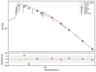
Figure 7: Kurucz stellar spectrum for a star with $T_{\mathrm{eff}}$ = 9500 K and log g =5.0 (grey line), the synthetic SED compute with the Kuzucz model (colored diamonds) and the observational SED (black dots). The lower panel show residuals between synthetic photometries and the SED in number of $\sigma$.

Appendix B MCMC analysis of the DDiT model