¹¹³Cd $\beta$-decay spectrum and $g_{\rm A}$ quenching using spectral moments

Abstract

We present an alternative analysis of the ¹¹³Cd $\beta$-decay electron energy spectrum in terms of spectral moments $\mu_{n}$, corresponding to the averaged values of $n^{\rm th}$ powers of the $\beta$ particle energy. The zeroth moment $\mu_{0}$ is related to the decay rate, while higher moments $\mu_{n}$ are related to the spectrum shape. The here advocated spectral-moment method (SMM) allows for a complementary understanding of previous results, obtained using the so-called spectrum-shape method (SSM) and its revised version, in terms of two free parameters: $r=g_{\rm A}/g_{\rm V}$ (the ratio of axial-vector to vector couplings) and $s$ (the small vector-like relativistic nuclear matrix element, $s$-NME). We present numerical results for three different nuclear models with the conserved vector current hypothesis (CVC) assumption of $g_{\rm V}=1$. We show that most of the spectral information can be captured by the first few moments which are simple quadratic forms (conic sections) in the $(r,\,s)$ plane: an ellipse for $n=0$ and hyperbolae for $n\geq 1$, all being nearly degenerate as a result of cancellations among nuclear matrix elements. The intersections of these curves, as obtained by equating theoretical and experimental values of $\mu_{n}$, identify the favored values of $(r,\,s)$ at a glance, without performing detailed fits. In particular, we find that values around $r\sim 1$ and $s\sim 1.6$ are consistently favored in each nuclear model, confirming the evidence for $g_{\rm A}$ quenching in ¹¹³Cd, and shedding light on the role of the $s$-NME. We briefly discuss future applications of the SMM to other forbidden $\beta$-decay spectra sensitive to $g_{\rm A}$.

I Introduction

The search for the rare process of neutrinoless double beta decay ($0\nu\beta\beta$), as well the study of its implications for the fundamental nature of the neutrino field (Dirac or Majorana), represent a major topic in both particle and nuclear physics Adams:2022jwx ; Agostini:2022zub ; Cirigliano:2022oqy . The predicted rate of this decay, as well as of other weak-interaction nuclear processes, depends sensitively on the effective value of the weak axial-vector coupling $g_{\rm A}$ that, in nuclear matter, appears to be generally different Suhonen:2017krv ; Suhonen:2019qcd from the vacuum value $g_{\rm A}^{\mathrm{vac}}=1.276$ UCNA:2010les ; Mund:2012fq . In particular, effective quenching factors $q=g_{\rm A}/g_{\rm A}^{\mathrm{vac}}<1$ have been discussed in a variety of observed $\beta$ and $\beta\beta$ decays, whose Gamow-Teller (GT) nuclear matrix elements are reduced by factors of $q$ and $q^{2}$, respectively; see, e.g., Suhonen:2017krv ; Suhonen:2019qcd ; Chou:1993zz ; Faessler:2007hu ; Barea:2013bz ; Ejiri:2019lfs .

While the theoretical connections among disparate values of $q$ and their physical origin are still subject to research Suhonen:2017krv ; Ejiri:2019ezh ; Gysbers:2019uyb ; Cirigliano:2022rmf , from a phenomenological viewpoint it makes sense to study observables that appear to be particularly sensitive to possible quenching effects. In this context, highly forbidden non-unique $\beta$-decays offer a very interesting avenue, since both their calculated decay rates and energy-spectrum shapes are found to change very rapidly around quenched values $g_{\rm A}\sim 1$, due to subtle cancellations among large nuclear matrix elements Haaranen:2016rzs .

For the fourth-forbidden non-unique $\beta$ decay of ¹¹³Cd, detailed experimental data are available for the energy spectrum $S(w_{e})$ in terms of the $\beta$ energy $w_{e}$ Belli:2007zza ; COBRA:2018blx . The data constrain both the overall decay rate (or, analogously, the half-life) and the energy spectrum shape (as a function of $w_{e}$). It is highly nontrivial to match the corresponding theoretical predictions with data, since the values of $g_{\rm A}$ that best fit the decay half-life are not necessarily the same that best fit the decay spectral shape and may be in conflict Haaranen:2016rzs ; COBRA:2018blx ; Haaranen:2017ovc , although both indicate large NME cancellations. These two approaches to constraining $g_{\rm A}$ in ¹¹³Cd $\beta$ decay, dubbed as half-life and spectrum-shape methods Haaranen:2017ovc , have only recently been reconciled by varying a small parameter multiplied by the vector coupling $g_{\rm V}$, namely, the so-called small relativistic nuclear matrix element $s$-NME Kostensalo:2020gha (${}^{V}\!{\cal{M}}^{(0)}_{431}$ in the notation of Behrens and Bühring Behrens1982 ), the estimates of which, from the conserved vector current (CVC) hypothesis or based on specific nuclear models, are rather uncertain but crucial for forbidden decays Kirsebom:2019tjd ; Kumar:2020vxr .

In particular, by treating the $s$-NME as a free parameter to be determined by data in a revised version of the spectrum-shape method (SSM) Kostensalo:2020gha , both the ¹¹³Cd half-life and spectrum data in Kostensalo:2020gha ; Dawson:2009ni have been found to match well the theoretical predictions of different models, with consistent values of the quenching factor and the $s$-NME. These nontrivial results, which represent a strong indication for $g_{\rm A}$ quenching in ¹¹³Cd, deserve in our opinion further analysis, aiming at a better understanding of the comparison of theory and data, in light of recent and future investigations of forbidden $\beta$-decay spectra in other nuclides Kumar:2020vxr ; Kostensalo:2017jgw ; Leder:2022beq . In particular, we aim at reducing the relevant spectral information to a relatively small set of quantities or parameters to be studied.

We start from the basic property that any smooth spectrum $S(w_{e})$ can be characterized by (and reconstructed from) the series of its moments $\mu_{n}$, namely, by the spectrum-averaged values of $w_{e}^{n}$ for $n\geq 0$ Feller91 ; Shohat70 . This approach to spectra allows for the unification of the half-life method (connected to $\mu_{0}$) and the SSM (connected to $\mu_{1,2,3,...}$) in a single “spectral-moment method (SMM).” We show that a few moments $\mu_{n}$ can capture with high accuracy the whole spectral information in terms of the two free parameters, $r=g_{\rm A}/g_{\rm V}$ and $s=s$-NME, where $g_{\rm V}$ is the vector coupling (assumed to be unity as in Kostensalo:2020gha ). Furthermore, since the moments $\mu_{n}$ are simple quadratic forms in $(r,\,s)$, the information contained in the infinite family of spectra $S(w_{e}\,|\,r,\,s)$ can be eventually discretized, with significant conceptual and numerical advantages.

Concerning experimental data, herein we use the absolute ¹¹³Cd $\beta$-decay spectrum of Belli:2007zza including the energy calibration and systematics assessment performed in Belli:2019bqp . Constraints on $(r,\,s)$, as obtained by comparing theoretical and experimental moments, are interpreted in terms of intersections of iso-moment curves (an ellipse for $\mu_{0}$ and hyperbolae for $\mu_{1,2,3,...}$). In each of three different nuclear models for the NME, such intersections are closest for rather similar values of the $(r,\,s)$ parameters. Since most of the relevant features appear to be captured by just the first few moments, the method can be pragmatically applied to future forbidden $\beta$-decay measurements in different nuclei, where the available spectral data might be more limited than for ¹¹³Cd.

Our work is structured as follows. In Sec. II we discuss the spectral-moment method, the adopted notation, and the numerical values of the first few moments. In Sec. III we discuss the implications of equating the theoretical and experimental moments in terms of the $(r,\,s)$ parameters. We find evidence for $r\sim 1$, corresponding to a multiplicative renormalization of the axial-vector coupling, as well as for $|s|\sim 1.6$ (with a preference for positive values of $s$), corresponding to an additive contribution to vector-like NME, consistent with earlier findings utilizing a different approach and independent data Kostensalo:2020gha . We summarize our results and consider further applications of the SMM in Sec. IV. Technical aspects about NMEs and quadratic forms are discussed in Appendix A and B, respectively.

II Spectral moments: method, notation and numerical values

In this Section we define the notation used in the SMM to describe the ¹¹³Cd $\beta$-decay spectra (experimental and theoretical) in terms of a truncated set of spectral moments. Numerical values for such moments are also derived.

II.1 $\beta$-decay spectrum notation

Following Haaranen:2016rzs ; Haaranen:2017ovc ; Kostensalo:2020gha , we introduce a dimensionless energy parameter $w_{e}$,

$$w_{e}=\frac{W_{e}}{m_{e}}=1+\frac{T_{e}}{m_{e}}\ ,$$ (1)

where $W_{e}$ and $T_{e}$ are, respectively, the total and kinetic energies of the electron with mass $m_{e}$.

The energy spectrum $S(w_{e})$ is defined as the fractional number of decays $n_{e}$ per single nucleus and per unit of time $t$ and of energy $w_{e}$

$$S(w_{e})=\frac{d^{2}n_{e}}{dt\,dw_{e}}\ ,$$ (2)

where $w_{e}\in[1,\,w_{0}]$, and the endpoint $w_{0}$ is set by the $Q_{\beta}$-value of the decay ($w_{0}=1+Q_{\beta}/m_{e}$). When needed, experimental ($e$) and theoretical ($t$) spectra are distinguished by superscripts,

$$S^{e} = S^{\mathrm{expt}},$$ (3)

$$S^{t} = S^{\mathrm{theo}}\ .$$ (4)

In order to link our formalism with common nuclear physics notation, we remind that the total decay rate $\lambda$ (or, equivalently, the half life $t_{1/2}$) is obtained by integrating $S(w_{e})$ over the interval $[1,\,w_{0}]$:

$$\lambda=\int_{1}^{w_{0}}S(w_{e})\,dw_{e}=\frac{\ln 2}{t_{1/2}}\ .$$ (5)

However, we shall not use either $\lambda$ or $t_{1/2}$ hereafter, for the following reason.

Due to increasingly high backgrounds at low energy, the experimental spectrum is typically reported above a detector-dependent kinetic energy threshold $T_{\rm thr}>0$ Belli:2007zza ; COBRA:2018blx ; Kostensalo:2020gha ; Belli:2019bqp that defines the $w_{e}$ threshold as $w_{\rm thr}=1+T_{\rm thr}/m_{e}>1$. Therefore, the decay half life $t_{1/2}$ can be estimated only by extrapolating the measured $S^{e}$ spectrum down to $T\to 0$, see e.g. Belli:2007zza . However, any adopted extrapolation function may well be different from the computed theoretical spectra in the range $[1,\,w_{\rm thr}]$ below threshold. In order to avoid potential biases, we shall thus consistently compare the experimental and theoretical spectra only in the energy range above threshold,

$$w_{e}\in[w_{\rm thr},\,w_{0}]\ .$$ (6)

II.2 Spectral moments $\mu_{n}$

It is well known from statistics that a smooth spectrum $S(w_{e})$, defined over an interval $w_{e}\in[w_{\rm thr},\,w_{0}]$, can be described by a series of moments $\{\mu_{n}\}_{n\geq 0}$ Feller91 ; Schmudgen17 . The zeroth moment, defined as

$$\mu_{0}=\int_{w_{\rm thr}}^{w_{0}}S(w_{e})\,dw_{e}\ ,$$ (7)

encodes the overall spectrum normalization, while the first and higher moments, defined as

$$\mu_{n}=\frac{\int_{w_{\rm thr}}^{w_{0}}S(w_{e})\,w_{e}^{n}\,\,dw_{e}}{\int_{w_{\rm thr}}^{w_{0}}S(w_{e})\,dw_{e}}\ (n\geq 1)\ ,$$ (8)

encode the spectrum shape information, via the averaged values of increasingly high powers of the main variable.

Note that, in our case, $\mu_{0}$ has the dimension of an inverse time, being defined as the decay rate in the interval $[w_{\rm thr},\,w_{0}]$ above threshold (see also Eq. (5) for the total rate in $[1,\,w_{0}]$). All the other moments are instead dimensionless. When needed, moments of theoretical and experimental spectra will be distinguished by superscripts:

$$S=S^{t} \to \mu_{n}=\mu_{n}^{t}\ ,$$ (9)

$$S=S^{e} \to \mu_{n}=\mu_{n}^{e}\ .$$ (10)

There is a vast and interdisciplinary literature on the inverse moment problem, namely, on possible methods to reconstruct the original function $S(w_{e})$ from a finite number of moments $\{\mu_{n}\}_{n=0,\dots,N}$ with some approximations Akhiezer20 ; Shohat70 ; Talenti87 . While all methods tend to improve their accuracy for increasing $N$, some may converge faster or better than others, depending on specific features of the function(s) $S(w_{e})$.

We have checked that a simple reconstruction algorithm based on an expansion in Legendre polynomials, as described in Askey82 , is sufficient enough to allow for the reconstruction of the ¹¹³Cd spectra at subpercent level (more accurately than is needed for our purposes) in the entire parameter space relevant for this work, with just $N=6$ moments. Representative examples of theoretical spectra reconstructed from a finite set of moments are shown below in Sec. II.4. Such results are consistent with (but more general than) the findings of Ref. Belli:2007zza , where the experimental spectrum was well approximated in terms of a 6^th order polynomial function.

We shall thus limit ourselves to $N=6$ and consider the truncated set of moments

$$\{\mu_{n}\}=\mu_{0},\,\mu_{1},\dots,\,\mu_{6}\ .$$ (11)

Actually, as we shall see in several ways, interesting results can be obtained by considering just the first two or three moments out of the above set.

II.3 Experimental spectrum $S^{e}(w_{e})$

In this work we consider the experimental spectrum $S_{e}(w_{e})$ of ¹¹³Cd as measured in Belli:2007zza , after a recalibration of the energy scale and the deconvolution of resolution effects as described in Belli:2019bqp (see Fig. 29 therein). The experimental threshold $T_{\rm thr}=26$ keV Belli:2019bqp and the endpoint $Q_{\beta}=323.83$ keV AME2016 define the analysis range:

$$w_{e}\in[w_{\rm thr},\,w_{0}]=[1.051,\,1.634]\ .$$ (12)

In this range, the experiment observed $N_{e}=2.222\times 10^{6}$ events for $N_{d}=8.858\times 10^{22}$ decaying nuclei over a data-taking time $t=9.929\times 10^{6}$ s Belli:2007zza ; Belli:2019bqp . The corresponding decay rate provides the zeroth moment $\mu^{e}_{0}=N_{e}/(N_{d}\,t)$:

$$\mu_{0}^{e}=2.526\times 10^{-24}\,\mathrm{s}^{-1}\ .$$ (13)

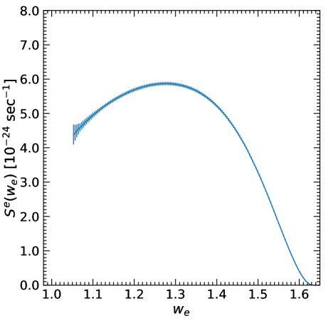
Figure 1: Experimental energy spectrum for ¹¹³Cd $\beta$ decay (central values and total $1\sigma$ errors) as taken from Belli:2019bqp . See the text for details.

Figure 1 shows the experimental spectrum in the range of Eq. (12), as taken from Belli:2019bqp with the above normalization. The spectrum is reported in bins of width $\Delta w_{e}=2~{}\mathrm{keV}/m_{e}$, together with total (statistical and systematic) uncertainty in each bin.

From the above $S^{e}(w_{e})$ we derive the following values for the experimental moments (up to $N=6$):

$$\mu^{e}_{1} = 1.291\ ,$$ (14)

$$\mu^{e}_{2} = 1.686\ ,$$ (15)

$$\mu^{e}_{3} = 2.226\ ,$$ (16)

$$\mu^{e}_{4} = 2.970\ ,$$ (17)

$$\mu^{e}_{5} = 4.004\ ,$$ (18)

$$\mu^{e}_{6} = 5.452\ .$$ (19)

We postpone the discussion of related uncertainties to Sec. III.

A final comment is in order. In Belli:2007zza , by extrapolating the observed spectrum below threshold (i.e., for $w_{e}\in[1,\,1.051]$), the total number of decays was estimated to be $N^{\prime}_{e}=2.40\times 10^{6}$ for the exposure $N_{d}\,t$, corresponding to a decay rate $\lambda=N^{\prime}_{e}/(N_{d}\,t)=2.73\times 10^{-24}$ s^-1 and to the quoted half-life $t_{1/2}=\ln 2/\lambda=8.04\times 10^{15}$ y. As previously mentioned, we do not use extrapolated quantities such as $\lambda$ or $t_{1/2}$ in this work.

II.4 Theoretical spectrum $S^{t}(w_{e})$ and its free parameters $(r,\,s)$

As discussed in Haaranen:2017ovc and references therein, the theoretical $\beta$-decay spectrum $S^{t}(w_{e})$ can be generally expressed as

$$S^{t}(w_{e})=\frac{\ln 2}{\kappa}\,C(w_{e})\,p\,w_{e}\,(w_{0}-w_{e})^{2}\,F_{0}(Z,\,w_{e})\ ,$$ (20)

where $C(w_{e})$ is the so-called shape factor, $p$ is the electron momentum in units of $m_{e}$, and $F_{0}(Z,\,w_{e})$ is the Fermi function with the final nuclear state having $Z=49$. In contexts where extreme precision is required, small correction terms accounting for, e.g., radiative effects and atomic screening become important. For the purposes of this work these $\approx 1\%$ corrections are insignificant but have been included as described in Haaranen:2017ovc . The conversion constant $\kappa$ reads:

$$\kappa=\frac{2\pi^{3}\ln 2}{m_{e}^{5}\,(G_{F}\,\cos\theta_{C})^{2}}=6289\ \mathrm{s}\ ,$$ (21)

where $G_{F}$ is the Fermi constant and $\theta_{C}$ is the Cabibbo angle. For non-unique decays the shape factor has a complicated expression including universal kinematic factors and nuclear matrix elements (NME). The latter capture all the nuclear-structure dependent information regarding the decay. In the formalism of Behrens and Bühring Behrens1982 the NME arise from a multipole expansion of the nuclear current. The NME are then expanded as a power series resulting in an expression including vector NME ${}^{V}\!{\cal{M}}^{(m)}_{KLs}$ and axial-vector NME ${}^{A}\!{\cal{M}}^{(m)}_{KLs}$. The matrix elements with the smallest angular momenta $K$ and $L$ allowing for the decay dominate, with the first term in the power series, $m=0$, being by far the most important. For fourth-forbidden unique decays there are four leading-order NME, with the dominant matrix elements being ${}^{V}\!{\cal{M}}^{(0)}_{440}$ and ${}^{A}{\cal{M}}^{(0)}_{441}$, and with significantly smaller contributions coming from ${}^{V}\!{\cal{M}}^{(0)}_{431}$ and ${}^{A}\!{\cal{M}}^{(0)}_{541}$. The expansion can be further carried out to next-to-leading order, resulting in a total of 45 NME Haaranen:2017ovc that depend on $w_{e}$ and on powers of the nuclear radius $R=1.2\,A^{1/3}\ \mathrm{fm}=5.8\ \mathrm{fm}$. The NME need to be numerically computed with specific nuclear models. Following Haaranen:2017ovc ; Kostensalo:2020gha we consider: the microscopic interacting boson-fermion model (IBFM-2), the microscopic quasiparticle-phonon model (MQPM), and the interacting shell model (ISM). First we discuss general aspects of the spectrum structure, and then report model-dependent numerical results in terms of spectral moments.

In general, $C(w_{e})$ is a sum over squares and products of linear combinations of NME, each being multiplied by either the vector coupling $g_{\rm V}$ or the axial-vector coupling $g_{\rm A}$. The couplings arise in the formalism of beta decays as a means to normalize the hadron current when moving from the quark level to the level of nucleons, and each axial-vector matrix element is always preceded by $g_{\rm A}$ and each vector matrix element by $g_{\rm V}$. By defining the ratio

$$r=g_{\rm A}/g_{\rm V}$$ (22)

one can formally write $S^{t}(w_{e})$ as a quadratic form in $r$ Haaranen:2016rzs ,

$$S^{t}=g_{\rm V}^{2}(S^{t}_{\rm V}+rS^{t}_{\rm VA}+r^{2}S^{t}_{\rm A})\ ,$$ (23)

where $S^{t}_{\rm A}$ includes only axial-vector NME, $S^{t}_{\rm V}$ only vector NME, and $S^{t}_{\rm VA}$ is a mix of vector and axial-vector NME. Hereafter we shall assume as in Kostensalo:2020gha , in accordance with the conserved vector current (CVC), that

$$g_{\rm V}=1\ ,$$ (24)

while $r$ will be treated as a free theoretical parameter to be fixed by the data. We shall comment on deviations from Eq. (24) in Sec. III.

As discussed in detail in Haaranen:2017ovc , the quadratic form in Eq. (23) entails delicate cancellations among large NME for $r\sim 1$, where agreement between theory and data can be usually found in terms of either the spectrum normalization Haaranen:2016rzs or its shape COBRA:2018blx , but not both at the same time (as far as $r$ is the only free parameter) Haaranen:2016rzs ; Haaranen:2017ovc . In particular, the main NME cancellation term turns out to be the square of a binomial, up to subleading NME terms $\epsilon$ and $\epsilon^{\prime}$:

$$S^{t}\propto\left({}^{V}\!{\cal{M}}^{(0)}_{440}-\alpha\,{}^{A}\!{\cal{M}}^{(0)}_{441}\,r+\epsilon\right)^{2}+\epsilon^{\prime}$$ (25)

where $\alpha$ is a numerical coefficient of $O(1)$ and the $\cal{M}$’s are “large” NME, tipically of $O(10^{2})$–$(10^{3})$ in units of fm⁴; see Haaranen:2017ovc for details of the notation and for numerical $\cal{M}$ values in the various nuclear models. For $r\sim 1$, it turns out that the two large $\cal{M}$’s tend to cancel each other, leaving a residual of $O(1)$ Haaranen:2017ovc . Therefore, a subleading term $\epsilon\sim O(1)$ may still play a significant role, especially if its numerical value is rather uncertain.

It was realized in Kirsebom:2019tjd ; Kumar:2020vxr ; Kostensalo:2020gha that this role can be played by so-called small relativistic NME, dubbed as $s$-NME in Kostensalo:2020gha and here just as $s$ for simplicity, where:

$$s={}^{V}\!{\cal{M}}^{(0)}_{431}\ ,$$ (26)

in units of fm³. On the one hand, with very simple (though unrealistic) assumptions related to the nuclear-structure aspects of the decay, the CVC hypothesis would imply (in our adopted units) the numerical relation ${}^{V}\!{\cal{M}}^{(0)}_{431}=0.0678(R^{-1}){}^{V}\!{\cal{M}}^{(0)}_{440}$ Kostensalo:2020gha , leading to expected values $s\sim O(1$–$10)$. On the other hand, numerical evaluations of $s$ either give $s=0$ due to model-specific limitations relating to a restricted model space (in the IBFM-2 and ISM models) or to $s\simeq 0.4$ (in the MQPM model) Haaranen:2017ovc . A more detailed discussion of the uncertain estimates of $s={}^{V}\!{\cal{M}}^{(0)}_{431}$ as compared with ${}^{V}\!{\cal{M}}^{(0)}_{440}$ and ${}^{A}\!{\cal{M}}^{(0)}_{441}$ is presented in Appendix A.

Given such uncertainties, in Kostensalo:2020gha the $s$-NME was simply assumed as a free parameter, presumably of $O(1)$, to be constrained by comparison with the data (together with $g_{\rm A}$). It turns out that, in this way, both the experimental spectrum shape and its normalization can be well reproduced theoretically Kostensalo:2020gha . In the same spirit, we treat $(r,\,s)$ as free parameters in our analysis.

Figure 2 shows three representative theoretical spectra $S^{t}(w_{e})$ calculated in the IBFM-2 model (dashed lines) for three different $(r,\,s)$ values. Their accurate reconstruction through a set of moments truncated at $N=6$ is also shown in the left panel (dotted lines). Analogously, the right panel shows the reconstruction truncated at $N=2$: it can be seen that the main qualitative features of the spectra are already captured by using just the first three moments $\mu_{0}$, $\mu_{1}$ and $\mu_{2}$. Similar results hold for the spectra calculated in the MQPM and ISM models (not shown). The analysis in Sec. III will confirm that, in general, a few moments are enough to derive useful indications on the $(r,\,s)$ parameters.

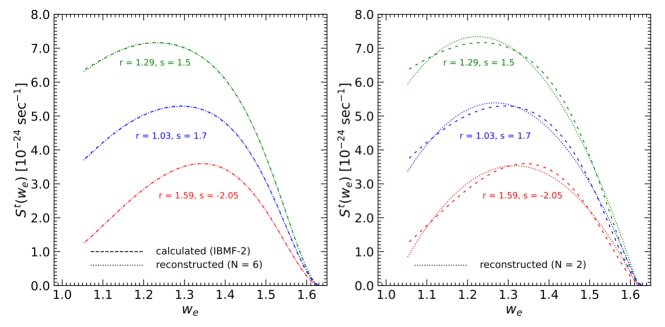
Figure 2: Representative examples of theoretical spectra $S^{t}$ as calculated in the IBFM-2 model (dashed lines), for three representative pairs of the $(r,\,s)$ parameters. The reconstruction of the spectra based on a truncated set of moments is also shown (dotted lines) for $N=6$ (left panel) and $N=2$ (right panel).

In particular, by using as free parameters both $r$ and $s$, it appears from Fig. 2 that one can alter both the peak position and the normalization of the theoretical spectrum, and may thus hope to match the experimental spectrum in Fig. 1. It turns out that this result is achieved for typical values $r\sim 1$ (confirming $g_{\rm A}$ quenching) and $s\sim O(1)$ (in the expected numerical ballpark), where the large NME cancellations mentioned in the context of Eqs. (25,26) take place. We shall recover very similar results, not only by using an independent data set Belli:2007zza ; Belli:2019bqp (as reported in Fig. 1), but by adopting a different perspective, based on the following generalization of the quadratic form in Eq. (23).

We observe that, since $s$ adds to the NME terms multiplied by $g_{\rm V}$, it must appear up to second power in $S^{t}(\omega)$. Moreover, a mixed dependence $\propto r\cdot s$ must emerge from the VA term in Eq. (23). Therefore, the spectrum $S^{t}(w_{e})$ must be a quadratic form in both $r$ and $s$, as well as any integral over it involving $w_{e}^{n}$ (with $n\geq 0$),

$$\int_{w_{\rm thr}}^{w_{0}}S^{t}(w_{e})\,w_{e}^{n}\,dw_{e}=\sum_{i+j\leq 2}a^{n}_{ij}\,r^{i}\,s^{j}\ ,$$ (27)

where the numerical coefficients $a^{n}_{ij}$ (with $n$ being a superscript, not a power) are expressed in units of s^-1 as the spectrum $S^{t}$. The $0^{\rm th}$ moment $\mu^{t}_{0}(r,\,s)$ corresponds to the above quadratic form with $n=0$, while the $n^{\rm th}$ moment $\mu^{t}_{n}(r,\,s)$ for $n\geq 1$ corresponds to a ratio of quadratic forms (with index $n$ at numerator and zero at denominator).

In practice, to evaluate the $a^{n}_{ij}$ coefficients for a given nuclear model at fixed $n$, one just needs to calculate the energy spectrum $S^{t}(w_{e}\,|\,r,\,s)$ at six arbitrary points $(r,\,s)$, evaluate the integral on the l.h.s. of Eq. (27), and solve in the six unknowns $\{a^{n}_{ij}\}$. Table 1 reports the numerical $\{a^{n}_{ij}\}$ values (in units of $10^{-24}$ s^-1) up to $N=6$, for the three nuclear models discussed in this work.

Table 1: Coefficients $a^{n}_{ij}$ of the quadratic forms parametrizing the theoretical moments up to $N=6$, in each of the three nuclear models considered in this work. The $a^{n}_{ij}$ are expressed in units of $10^{-24}$ s^-1.

Model	$n$	$a^{n}_{20}$	$a^{n}_{02}$	$a^{n}_{11}$	$a^{n}_{10}$	$a^{n}_{01}$	$a^{n}_{00}$
	0	$+2.8998$	$+0.7914$	$+2.8163$	$-5.8662$	$-2.9952$	$+3.1087$
	1	$+3.6046$	$+1.0225$	$+3.5722$	$-7.2731$	$-3.7984$	$+3.8552$
	2	$+4.5331$	$+1.3358$	$+4.5835$	$-9.1214$	$-4.8722$	$+4.8357$
IBFM-2	3	$+5.7690$	$+1.7640$	$+5.9492$	$-11.574$	$-6.3214$	$+6.1368$
	4	$+7.4305$	$+2.3542$	$+7.8102$	$-14.862$	$-8.2949$	$+7.8803$
	5	$+9.6855$	$+3.1738$	$+10.368$	$-19.312$	$-11.005$	$+10.239$
	6	$+12.774$	$+4.3204$	$+13.912$	$-25.390$	$-14.758$	$+13.460$
	0	$+20.086$	$+0.7914$	$+7.5565$	$-41.059$	$-7.8113$	$+21.146$
	1	$+24.911$	$+1.0225$	$+9.5846$	$-50.905$	$-9.9058$	$+26.223$
	2	$+31.253$	$+1.3358$	$+12.298$	$-63.839$	$-12.706$	$+32.892$
MQPM	3	$+39.676$	$+1.7640$	$+15.962$	$-81.005$	$-16.485$	$+41.740$
	4	$+50.976$	$+2.3542$	$+20.955$	$-104.01$	$-21.632$	$+53.598$
	5	$+66.281$	$+3.1738$	$+27.817$	$-135.15$	$-28.700$	$+69.640$
	6	$+87.205$	$+4.3204$	$+37.325$	$-177.68$	$-38.485$	$+91.542$
	0	$+17.509$	$+0.7914$	$+7.0682$	$-33.572$	$-6.8313$	$+16.166$
	1	$+21.713$	$+1.0225$	$+8.9655$	$-41.627$	$-8.6632$	$+20.050$
	2	$+27.238$	$+1.3358$	$+11.504$	$-52.208$	$-11.113$	$+25.151$
ISM	3	$+34.576$	$+1.7640$	$+14.932$	$-66.252$	$-14.418$	$+31.919$
	4	$+44.418$	$+2.3542$	$+19.603$	$-85.078$	$-18.920$	$+40.990$
	5	$+57.748$	$+3.1738$	$+26.024$	$-110.56$	$-25.103$	$+53.262$
	6	$+75.969$	$+4.3204$	$+34.920$	$-145.36$	$-33.663$	$+70.018$

Summarizing, we have discretized the continuous information contained in the infinite family of spectra $S^{t}(w_{e}\,|\,r,\,s)$ into a small number of moments $\mu_{n}^{t}$, each depending on simple quadratic forms in the free parameters $r$ and $s$ (involving six coefficients $a^{n}_{ij}$ at any $n$). This approach greatly simplifies the numerical calculation of the theoretical moments, as well as their comparison with the experimental moments $\mu_{n}^{e}$, as discussed below.

III Spectral moment method: Comparison of theory and data

In this Section we explore the implications of equating a finite set of theoretical and experimental moments:

$$\mu^{t}_{n}(r,\,s)=\mu^{e}_{n}\ (n=0,\,1,\dots N)\ .$$ (28)

Each of the above equations sets a quadratic form in $(r,\,s)$ equal to a constant, and thus leads to a conic section in the corresponding coordinates. It turns out that, for $n=0$, the conic section is a slanted and elongated ellipse, while for $n\geq 1$ the conics form a bundle of hyperbolae. In the ideal case (perfect match between theory and data), all these curves would intersect in a single $(r,\,s)$ point; in real cases, the various crossing points will cluster with some dispersion around a preferred $(r,\,s)$ region. The smaller the dispersion, the better the agreement between the experimental and theoretical moments and spectra. In Appendix B we discuss general features of the conic sections and of their crossings, that allow to visualize the effects of large NME cancellations, as well as to interpret previous fit results obtained in Kostensalo:2020gha through the revised spectrum shape method. Below we show our results in the $(r,\,s)$ plane and discuss the preferred parameter values in the three nuclear models considered.

Figure 3 shows the loci of points in the $(r,\,s)$ plane fulfilling Eq. (28) up to $N=6$, for the model IBMF-2 (left), MQPM (middle), and ISM (right). In each panel, one can see (part of) the slanted ellipse determined by the zeroth moment, and the bundle of hyperbolae determined by the first and higher moments. The two regions where the ellipse and the bundle cross each other correspond to positive and negative values of $s$, and are enlarged in the lower set of panels. As discussed in Appendix B, in principle there are two other regions of crossing, close to the extremal sides of the ellipse and thus beyond scale (not shown), that would correspond to unphysical values of $r$ (much smaller or much larger than unity).

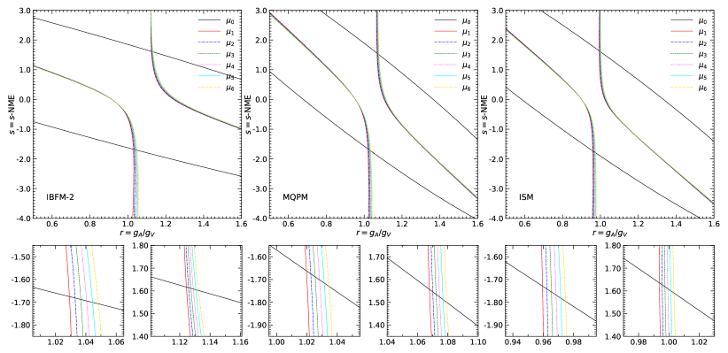
Figure 3: Numerical results obtained by imposing the equality of theoretical and experimental moments, $\mu_{n}^{t}=\mu_{n}^{e}$ (up to $N=6$) in the plane charted by the free parameters $r=g_{\rm A}/g_{\rm V}$ and $s=s$-NME. The left, middle and right plots correspond to the IBFM-2, MQPM and ISM models, respectively. In each of the three upper panels, note (part of) the slanted ellipse determined by the zeroth moment, and the bundle of hyperbolae determined by the first and higher moments. For each model, the two lower panels zoom in the regions at $s<0$ (left) and $s>0$ (right) where the ellipse and the bundle cross each other. See the text for details.

In each of the enlarged crossing regions reported in Fig. 3 (lower panels), the bundle of hyperbolae shows some dispersion, that turns out to be smaller for $s>0$ as compared with $s<0$, and minimal for the IBFM-2 model. Therefore, we expect that the experimental spectrum is best matched by the theoretical spectra at $s>0$ (w.r.t. $s<0$), in particular for the IBFM-2 model. For definiteness, we check these expectations by calculating the $S^{t}$ spectra at the points where the $\mu_{0}$ ellipse intersects the $\mu_{1}$ hyperbola, whose coordinates as reported in Table 2.

Table 2: Intersection points of the 0^th and 1^st moment curves in the $(r,\,s)$ plane, for each of the three nuclear models considered.

Model	$r$	$s$
IBFM-2	1.125	$+1.617$
	1.029	$-1.675$
MQPM	1.068	$+1.557$
	1.020	$-1.662$
ISM	0.994	$+1.635$
	0.960	$-1.729$

Figure 4 shows the theoretical spectra corresponding to the above $(r,\,s)$ values for the three nuclear models: IBFM-2 (left), MQPM (middle) and ISM (right). In each panel, the experimental spectrum (in light blue) should be compared with the blue-dashed and red-dotted spectra, referring to positive and negative values of $s$ in Table 2, respectively. The spectra with $s>0$ are generally slightly broader and less peaked than the experimental spectrum, while the opposite happens for the spectra with $s<0$. The deviations from the experimental spectrum are generally smaller for $s>0$ than for $s<0$. and can be as small as the experimental errors for the IBFM-2 model at $s>0$. In this context, we recall that the model IBFM-2 predicts a priori $s=0$ Haaranen:2017ovc , and that only by fixing $s\sim 1.6$ one gets the good agreement with the experimental data in Fig. 4; see Appendix A for details.

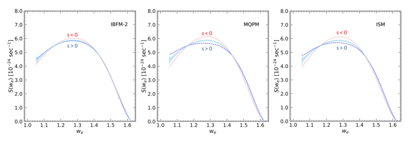
Figure 4: Theoretical spectra calculated at the $(r,\,s)$ points reported in Table 2, for each of the three nuclear models IBMF-2, MQPM and ISM (left, middle and right panels), as compared with the experimental spectrum of Fig. 1. In each panel, the dashed blue curve refers to the case $s>0$, and the dotted red curve to the case $s<0$.

We thus find that all models point towards $r\sim 1$, corresponding to a quenching factor $q=g_{\rm A}/g_{\rm A}^{\mathrm{vac}}\sim 0.8$ assuming $g_{\rm V}=1$; and towards $|s|\simeq 1.6$, corresponding to a small vector-like relativistic NME in the expected ballpark of $O(1)$, with a preference for $s>0$. More precisely, by grouping the values in Table 2, we find the best match between theory and data around

$$r \simeq 0.99-1.13\ ,$$ (29)

$$s \simeq 1.56-1.64\ ,$$ (30)

with a secondary (worse) match around $r\simeq 0.96$–$1.03$ and $s=-(1.66$–$1.73)$, that cannot be excluded a priori from a phenomenological viewpoint (see also Appendix A). Remarkably, the above ranges correspond to relatively small uncertainties on the $(r,\,s)$ parameters.

It would be tempting to refine the indications in favor of $r\sim 1$ and $|s|\sim 1.6$ by attaching more accurate error estimates to these parameters, as derived by detailed data fits including both experimental and theoretical uncertainties. However, in our case the theoretical shape errors are likely to be larger than the data errors (in contrast with the data analysis in Kostensalo:2020gha ), as suggested by the fact that, in Fig. 4, the theoretical spectra are generally outside (or at border of) the experimental error band. As a check, we have performed numerical least-squares adjustments of the theoretical spectra by including only experimental uncertainties, either by fitting the binned spectrum with uncorrelated total errors in Fig. 1 or by fitting the associated $N=6$ moments with their propagated covariance matrix. In both cases we obtain unreasonably high values of the minimum $\chi^{2}$ per d.o.f. (except for the noted IBFM-2 case at $s>0$), and unreasonably tiny errors on $(r,\,s)$ at subpercent level (in all cases), that are much smaller than the realistic few-percent spread of the same parameters (see Table 2). On the positive side, by using only experimental errors, the $(r,\,s)$ best fits are invariably close to the $s>0$ solutions reported in Eqs. (29,30) and their associated spectra are close to those in Fig. 4, within percent-level deviations (not shown). The SMM appears thus to provide reasonably correct and robust $(r,\,s)$ values, even with a limited amount of information and without the need for detailed data fits. Future improvements may include theoretical spectrum shape errors as estimated, e.g., by a detailed analysis of the inputs or approximations inherent the current next-to-leading order NME calculations in each nuclear model: a task that is beyond the scope of this work.

Similar results on $(r,\,s)$ were obtained in Kostensalo:2020gha , by applying a revised spectrum shape approach to an independent set of ¹¹³Cd $\beta$-decay data, characterized by a higher threshold ($T_{\rm thr}\simeq 52$–132 keV in different detectors, with $\langle T_{\rm thr}\rangle=92$ keV) with respect to the data used herein Belli:2007zza (having a single $T_{\rm thr}=26$ keV). In Kostensalo:2020gha , the preferred values for the free parameters were found to cluster around $g_{\rm A}\simeq 0.83$–$0.99$ (somewhat lower than our $g_{\rm A}\sim 0.99$–1.13) and around $s\simeq 1.85$–2.1 (somewhat higher than our $s\simeq 1.56$–1.64). We surmise that these differences may be due in part to the different ¹¹³Cd datasets and in part to the different approach used in the analysis. In particular, in this work the spectrum normalization is constrained through the 0^th moment (i.e., the absolute decay rate $\mu_{0}$ above the 16 keV threshold), while in Kostensalo:2020gha it is constrained through the decay half life (that requires a spectrum extrapolation below each of the 52–132 keV detector thresholds). As noted at the end of Section II.1, such extrapolations may lead to biases. Altering the normalization leads to anticorrelated changes between $g_{\rm A}$ and $s$ (as suggested by the $\mu_{0}$ ellipse in our approach), which is what we find in comparison with Kostensalo:2020gha . Apart from these differences, a robust message emerges from Kostensalo:2020gha and from this work: quenched values of the axial-vector coupling (around $g_{\rm A}\simeq 0.9$–1), accompanied by an adjustment of the small vector NME (around $s\simeq 1.6$–2), are required to match the existing ¹¹³Cd $\beta$-decay spectrum data in both normalization and shape, in each of the three nuclear models considered.

Around these $(r,\,s)$ values, large NME cancellations take place, leaving residual spectra that reasonably reproduce the experimental spectrum both in normalization (0^th moment) and in shape (1^st and higher moments). These phenomenological facts strongly suggest that all the models require the following adjustments: an overall multiplicative correction to the axial-vector NME, via a quenched value $g_{\rm A}\sim 1$ (for $g_{V}=1$); and a small additive vector-like correction, parametrized by a $s$-NME with an absolute value around $s\sim 1.6$. One might wonder whether $g_{\rm V}$ could be used as free parameters instead of $s$, abandoning the CVC assumption $g_{V}=1$. The answer is negative, since the prefactor $g^{2}_{\rm V}$ in Eq. (23) would only affect the zeroth moment $\mu_{0}$ but would cancel out in the first and higher moments [Eq. (8)], leading to a spectrum shape depending on a single free parameter $r$. It was already concluded in Haaranen:2016rzs that one cannot match both the spectrum normalization and its shape by varying just $g_{\rm V}$ besides $g_{\rm A}$. In other words, the additive adjustment parametrized by $s$ cannot be traded for a multiplicative adjustment parametrized by $g_{\rm V}$. At present, the CVC assumption $g_{\rm V}=1$ can thus be safely maintained in the context of ¹¹³Cd $\beta$ decay.

IV Summary and perspectives

In this work we have studied the normalization and shape of the electron energy spectrum of the fourth-forbidden $\beta$ decay of ¹¹³Cd with a novel approach, coined the spectral-moment method (SMM), based on a truncated set of spectral moments $\mu_{n}$. The 0^th moment is related to the normalization, while the 1^st and higher moments are related to the shape. As in Kostensalo:2020gha , we have assumed that the spectra depend on two free parameters: an axial-vector coupling parameter $r=g_{\rm A}/g_{\rm V}$ (for $g_{\rm V}=1)$ and a small relativistic vector-like NME parameter $s$. We have shown that: each moment is a quadratic form in $(r,\,s)$; iso-moment curves are ellipses for $\mu_{0}$ and hyperbolae for $\mu_{1,2,3\dots}$; the intersections of a few moment curves are enough to derive interesting constraints on $(r,\,s)$, without detailed data fits (see also Appendix B).

In particular, by equating the theoretical moments with the experimental ones, as derived from the data in Belli:2019bqp , the following results emerge: the intersection of the $\mu_{0}$ and $\mu_{1}$ curves provides $r\sim 1$ and $|s|\sim 1.6$; the case $s>0$ results in a smaller spread of intersections with higher-moment curves and is thus preferred, as also confirmed by visual inspection of the spectra. Nuclear model considerations also suggest $s\geq 0$, although $s<0$ cannot be excluded a priori (see also Appendix A). The spread of the $(r,\,s)$ values in Table 2, at the level of a few percent at least, exceeds the purely experimental uncertainties and call for (currently unquantified) theoretical spectrum-shape uncertainties. In any case, our results are in the same ballpark of those obtained in Kostensalo:2020gha with a different methodology and independent data. In general, the derived $(r,\,s)$ values provide evidence for a multiplicative renormalization (quenching) of the axial coupling $g_{\rm A}$ and for an additive adjustment of vector-like terms via the small relativistic $s$-NME.

Since the main quantitative information (apart from indications about the sign of $s$) has been derived just from $\mu_{0}$ and $\mu_{1}$, we surmise that the SMM can be quite powerful even when the experimental data are less accurate than those used in this work for ¹¹³Cd. In this context, it should be noted that ¹¹³Cd is just one of several nuclei where forbidden $\beta$ decays occur with a significant spectral dependence on $g_{\rm A}$ Haaranen:2016rzs ; Kostensalo:2017jgw ; Kostensalo:2017xxq ; Kumar:2021euw and possibly on other parameters such as the $s$-NME or similar ones.

In cases where the available spectral data are scarce, it should anyway be possible to derive, within a specified energy window $w_{e}\in[w_{e}^{\min},\,w_{e}^{\max}]$, at least the spectrum normalization $(\mu_{0})$ and the average energy $(\mu_{1})$ with reasonable approximation. By equating the experimental and theoretical values for these two moments, constraints on $(r,\,s)$ or equivalent parameters could be derived, without the need of complicated data fits. Among the forbidden $\beta$-decay spectra with significant $g_{\rm A}$ dependence, of particular importance is the ¹¹⁵In spectrum Haaranen:2016rzs , that was experimentally observed long ago in OldLi and recently measured with a bolometric detector in Leder:2022beq . A first data analysis with the spectrum-shape method (SSM), and using only $g_{\rm A}$ as a free parameter, suggests significant $g_{\rm A}$ quenching Leder:2022beq but does not account for both normalization and shape at the same time. It remains to be seen if allowance for an extra parameter such as the $s$-NME can provide a match to all data. The presently introduced SMM might allow a rapid check of this possibility, and will be applied to, e.g., existing ¹¹⁵In data in a separate work.

Appendix A Analysis of relevant NME

In the Tables 3–5 we have listed the single-particle (s.p.) matrix elements corresponding to all relevant transitions in the vector and axial-vector NME of interest for our analysis, namely, the small $s={}^{V}\!{\cal{M}}^{(0)}_{431}$ and the large (and largely cancelling) terms ${}^{V}\!{\cal{M}}^{(0)}_{440}$ and ${}^{A}\!{\cal{M}}^{(0)}_{441}$. The relevant pre-factors have been included so that these correspond to single-particle model NME and are thus comparable to the numerical NME values listed in Haaranen:2017ovc for ¹¹³Cd.

Table 3: The single-particle matrix elements ${}^{V}\!{\cal{M}}^{(0)}_{431}$ [fm³] for ¹¹³Cd for the relevant orbitals.

	$0f_{7/2}$	$0f_{5/2}$	$1p_{3/2}$	$1p_{1/2}$	$0g_{9/2}$	$0g_{7/2}$	$1d_{5/2}$	$1d_{3/2}$	$2s_{1/2}$	$0h_{11/2}$
$0f_{7/2}$	0	0	0	0	0	0	0	0	0	9.5
$0f_{5/2}$	0	0	0	0	0	0	0	0	0	-4.3
$1p_{3/2}$	0	0	0	0	0	0	0	0	0	-12.5
$1p_{1/2}$	0	0	0	0	0	0	0	0	0	0
$0g_{9/2}$	0	0	0	0	0	0	0	0	0	0
$0g_{7/2}$	0	0	0	0	0	0	0	0	0	0
$1d_{5/2}$	0	0	0	0	0	0	0	0	0	0
$1d_{3/2}$	0	0	0	0	0	0	0	0	0	0
$2s_{1/2}$	0	0	0	0	0	0	0	0	0	0
$0h_{11/2}$	-9.5	-4.3	12.5	0	0	0	0	0	0	0

Given that the initial and final states are ground states with spin-parities $1/2^{+}$ and $9/2^{+}$, respectively, the transition is most likely dominated by a transition between the neutron orbital $2s_{1/2}$ and the proton orbital $0g_{9/2}$. This means ${}^{V}\!{\cal{M}}^{(0)}_{431}$(s.p.)$=0$ fm³, ${}^{V}\!{\cal{M}}^{(0)}_{440}$(s.p.)$=637$ fm⁴, and ${}^{A}\!{\cal{M}}^{(0)}_{441}$(s.p.)$=565$ fm⁴. The nuclear models give ${}^{V}\!{\cal{M}}^{(0)}_{440}=$317–827 fm⁴, and ${}^{A}\!{\cal{M}}^{(0)}_{441}=$314–848 fm⁴, which are in reasonable agreement with the single-particle NME with the final values depending on contributions from other near-by orbitals. For ${}^{V}\!{\cal{M}}^{(0)}_{431}$ the situation is however very different, as no orbitals near the Fermi-surface have nonzero contributions. Furthermore, the CVC relation ${}^{V}\!{\cal{M}}^{(0)}_{431}=0.0678(R^{-1}){}^{V}\!{\cal{M}}^{(0)}_{440}$ mentioned in Sec. II.4 (which does not apply exactly when multiple configurations are allowed for the wave functions) suggests that ${}^{V}\!{\cal{M}}^{(0)}_{431}$(MQPM, CVC) = 9.7 fm³, ${}^{V}\!{\cal{M}}^{(0)}_{431}$(IBFM-2, CVC)=3.7 fm³, and ${}^{V}\!{\cal{M}}^{(0)}_{431}$(ISM) = 8.4 fm³, while the models give the values 0.37 fm³, 0 fm³, and 0 fm³, respectively. For the CVC values for the smallest NME to hold, the transition would need to be basically a pure $0h_{11/2}$-$1p_{3/2}$ which does not seem reasonable based on the spin-parities, the facts that these are ground states, and the proton and neutron numbers of the nuclei.

Table 4: The single-particle matrix elements ${}^{V}\!{\cal{M}}^{(0)}_{440}$ [fm⁴] for ¹¹³Cd for the relevant orbitals.

	$0f_{7/2}$	$0f_{5/2}$	$1p_{3/2}$	$1p_{1/2}$	$0g_{9/2}$	$0g_{7/2}$	$1d_{5/2}$	$1d_{3/2}$	$2s_{1/2}$	$0h_{11/2}$
$0f_{7/2}$	434	319	-363	-426	0	0	0	0	0	695
$0f_{5/2}$	-319	336	484	0	0	0	0	0	0	-306
$1p_{3/2}$	-363	-484	0	0	0	0	0	0	0	-907
$1p_{1/2}$	426	0	0	0	0	0	0	0	0	0
$0g_{9/2}$	0	0	0	0	729	382	-644	-397	637	0
$0g_{7/2}$	0	0	0	0	-382	621	452	-501	-570	0
$1d_{5/2}$	0	0	0	0	-644	-452	583	820	0	0
$1d_{3/2}$	0	0	0	0	397	-501	-820	0	0	0
$2s_{1/2}$	0	0	0	0	637	570	0	0	0	0
$0h_{11/2}$	695	306	-907	0	0	0	0	0	0	1111

.

Table 5: The single-particle matrix elements ${}^{A}\!{\cal{M}}^{(0)}_{441}$ [fm⁴] for ¹¹³Cd for the relevant orbitals.

	$0f_{7/2}$	$0f_{5/2}$	$1p_{3/2}$	$1p_{1/2}$	$0g_{9/2}$	$0g_{7/2}$	$1d_{5/2}$	$1d_{3/2}$	$2s_{1/2}$	$0h_{11/2}$
$0f_{7/2}$	0	500	-160	-475	0	0	0	0	0	-301
$0f_{5/2}$	500	0	-538	0	0	0	0	0	0	615
$1p_{3/2}$	160	-538	0	0	0	0	0	0	0	794
$1p_{1/2}$	-475	0	0	0	0	0	0	0	0	0
$0g_{9/2}$	0	0	0	0	0	774	-283	-624	565	0
$0g_{7/2}$	0	0	0	0	774	0	-704	222	632	0
$1d_{5/2}$	0	0	0	0	283	-704	0	911	0	0
$1d_{3/2}$	0	0	0	0	-624	-222	911	0	0	0
$2s_{1/2}$	0	0	0	0	-565	632	0	0	0	0
$0h_{11/2}$	301	615	-794	0	0	0	0	0	0	0

For ISM and IBFM-2 the value of ${}^{V}\!{\cal{M}}^{(0)}_{431}$ is systematically zero, as in the ISM calculations the orbital $0h_{11/2}$ was kept empty to reduce the large computational burden, and in IBFM-2 the initial state with spin-parity $1/2^{+}$ cannot be formed by pairing $0^{+}$ and $2^{+}$ bosons with a fermion with spin-parity $11/2^{-}$. For MQPM the contributions between $0h_{11/2}$ and the lower proton orbitals are included, but the contributions for the higher orbitals are not very reliable as the parameter tuning can be reasonably done only for the lowest orbitals.

Based on these arguments, we surmise that the $s$-NME is not well described by the nuclear models while the other NME do not suffer from the same problems. Therefore, it makes sense to take the $s$-NME as a tuning parameter instead of the large matrix elements. Concerning the sign of $s$, the option $s>0$ is theoretically regarded as being more reasonable Kostensalo:2020gha , since all the above estimates—despite being largely uncertain—typically provide $s\geq 0$. However, one cannot exclude a priori that $s<0$, also because some single-particle contributions may be negative (see Table 3).

Appendix B Quadratic forms in the $(r,\,s)$ parameters and conic sections

As mentioned in Sec. II.4 and discussed in Kostensalo:2020gha , in the $(r,\,s)$ region where theoretical and experimental spectra match, subtle cancellations in $S^{t}$ occur among large NME, with residuals modulated by smaller terms. Despite the complexity of the full $S^{t}$ expression at next-to-leading order Haaranen:2017ovc , some insights can be gained by elaborating upon Eqs. (25, 26), and by recalling that the moments are associated with quadratic forms in both $r$ and $s$.

The leading NME cancellation operating in $S^{t}$, as well as in its integral $\mu_{0}^{t}$, takes the form of a square of a large linear term in $r$, modulated by a smaller term in $s$. In first approximation, we thus expect the 0^th moment to take the form $\mu_{0}^{t}\simeq(a-br-cs)^{2}+d$, with $a$ and $b$ much larger than $c$ and $d$. In the plane charted by the $(r,\,s)$ parameters, the equation $\mu_{0}^{t}=\mu_{0}^{e}$ is then solved by two parallel straight lines with a small slope $-c/b$. In reality, due to subleading NME terms, the perfect square is altered into a more general quadratic form in $(r,\,s)$. Correspondingly, the two straight lines are just the degenerate limit of a conic section, which is actually an elongated and slanted ellipse.

Figure 5 (upper panel) reports graphically the above qualitative considerations in the plane charted by the $r$ and $s$ parameters. The elongated solid ellipse is the locus of points where $\mu_{0}^{t}=\mu_{0}^{e}$, i.e., where the normalization (event rate above threshold) of the experimental and theoretical spectra match, irrespective of their shapes that may be quite different. The dashed straight lines are a degenerate approximation of the ellipse.

While the spectrum normalization is associated to $\mu_{0}$, the spectrum shape is associated to higher moments, starting from $\mu_{1}$. Considering that $\mu_{1}$ is a ratio of quadratic forms, the constraint $\mu^{t}_{1}(r,\,s)=\mu^{e}_{1}$ leads to a quadratic equation as well, identifying another conic section that turns out to be a hyperbola. The appearance of a hyperbola for $\mu_{1}$ can be qualitatively understood as follows.

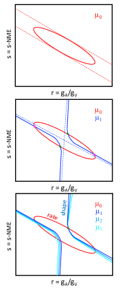
Figure 5: Qualitative expectations for the conic sections obtained by equating the theoretical and experimental moments in the $(r,\,s)$ plane (in arbitrary scales). Upper panel: ellipse associated to $\mu_{0}$, together with the degenerate limit (straight parallel lines). Middle panel: hyperbola associated to $\mu_{1}$, together with it asymptotes (roughly aligned along the vertical axis and the ellipse major axis); the hyperbola crosses the ellipse in four points (solutions). Lower panel: bundle of hyperbolae associated to $\mu_{1}$ and higher moments, crossing each other and the $\mu_{0}$ ellipse in a single point (marked with a dot).

Since the denominator and numerator of $\mu_{1}$ differ only by a $w_{e}$ integrand of $O(1)$ in the latter, [see Eq. (8)], the associated quadratic forms turn out to have nearly proportional coefficients (as confirmed by numerical inspection of Tab. 1), corresponding to geometrically similar ellipses upon rescaling. The scaling factor turns out to be slightly more pronounced along the abscissa $r$, that governs the main NME cancellation term. Roughly speaking, the equation $\mu^{t}_{1}(r,\,s)=\mu^{e}_{1}$ imposes that the ratio between two very similar elliptic forms (slightly differing along the abscissa) is close to unity. If one form is written as $x^{2}+y^{2}-2\rho xy$ (where $x$ and $y$ are generic coordinates), the other is thus obtained by scaling $x$ as $(1+\delta)x$, where $\delta\ll 1$. It is easy to check that, at first order in $\delta$, the ratio of these two forms is unity for either $x=0$ (corresponding to a vertical line) or for $x=\rho y$ (a slanted line, roughly along the ellipse major axis). These two lines define a degenerate hyperbola, coincident with its two asymptotes: a vertical one and a slanted one. In general, the equation $\mu^{t}_{1}(r,\,s)=\mu^{e}_{1}$ entails a less simplistic situation: the hyperbola defined by this equation is not exactly degenerate, and its asymptotes may be slightly tilted with respect to the above expectations.

Figure 5 (middle panel) reports graphically the typical locus of points where $\mu_{1}^{t}(r,\,s)=\mu_{1}^{e}$, i.e., where the average energies of the experimental and theoretical spectra do match. The locus is a hyperbola (blue solid curve), whose branches are relatively close to the degenerate limit (asymptotes, dashed lines). The hyperbola and the ellipse will cross in four points, i.e., there will be four different $(r,s)$ solutions to the coupled equations $\mu^{t}_{0}=\mu^{e}_{0}$ and $\mu^{t}_{1}=\mu^{e}_{1}$. In general, the extreme solutions in $r$ (red dots) correspond to unphysically low or high values of $g_{\rm A}$, and can be discarded a priori; the remaining two solutions (blue dots) typically correspond to negative and positive values of $s$.

With a reasoning similar to $\mu_{1}$, also the conic sections defined by the second or higher moments are expected to be hyperbolae. One then gets an ellipse for $n=0$ (related to the event rate) and a bundle of hyperbolas for $n\geq 1$ (related to the spectrum shape). If a perfect match between theory and data can be achieved, all these conic sections must intersect in just one of the four previous points, and diverge to some extent in the others. This case is shown in the lower panel of Fig. 5, assuming the solution marked by a dot. In reality, the theory-data match is never perfect, and the intersections will be slightly separated even in the best possible case.

The above discussion allows to understand some features of previous results reported in Kostensalo:2020gha by using the so-called revised SSM. This approach conflates the half-life and spectrum-shape methods (previously conflicting when using only $r$ as a free parameter, see e.g., Haaranen:2017ovc ), by treating $s$ as an additional degree of freedom. In particular, let us consider Fig. 2 of Kostensalo:2020gha , showing the results of fits to an independent ¹¹³Cd $\beta$-decay data set COBRA:2018blx in the plane charted by $g_{\rm A}$ and the $s$-NMA, for the same three nuclear models considered in our work. In that figure, while the half-life fit leads to an elliptical solution (akin to the ellipse determined by $\mu_{0}$ in our formalism), the spectrum shape fit leads to a band that crosses the ellipse. We can interpret such a band as the path taken by the fit algorithm in Kostensalo:2020gha to follow (and to fuzzily jump across) two half-branches of the bundle of higher-moment hyperbolae, the other two halves (leading to unphysical values of $g_{\rm A}$) being discarded by construction (the fit was also restricted to $s>0$ therein). With the spectral moment method discussed herein, the fit results in Kostensalo:2020gha can be understood in a unified picture.

References

- (1) C. Adams, K. Alfonso, C. Andreoiu, E. Angelico, I. J. Arnquist, J. A. A. Asaadi, F. T. Avignone, S. N. Axani, A. S. Barabash and P. S. Barbeau, et al. “Neutrinoless Double Beta Decay,” [arXiv:2212.11099 [nucl-ex]].
- (2) M. Agostini, G. Benato, J. A. Detwiler, J. Menéndez and F. Vissani, “Toward the discovery of matter creation with neutrinoless double-beta decay,” [arXiv:2202.01787 [hep-ex]].
- (3) V. Cirigliano, Z. Davoudi, W. Dekens, J. de Vries, J. Engel, X. Feng, J. Gehrlein, M. L. Graesser, L. Gráf and H. Hergert, et al. “Neutrinoless Double-Beta Decay: A Roadmap for Matching Theory to Experiment,” [arXiv:2203.12169 [hep-ph]].
- (4) J. T. Suhonen, “Value of the Axial-Vector Coupling Strength in and Decays: A Review,” Front. in Phys. 5, 55 (2017) [arXiv:1712.01565 [nucl-th]].
- (5) J. Suhonen and J. Kostensalo, “Double Decay and the Axial Strength,” Front. in Phys. 7, 29 (2019)
- (6) J. Liu et al. [UCNA], “Determination of the Axial-Vector Weak Coupling Constant with Ultracold Neutrons,” Phys. Rev. Lett. 105, 181803 (2010) [arXiv:1007.3790 [nucl-ex]].
- (7) D. Mund, B. Maerkisch, M. Deissenroth, J. Krempel, M. Schumann, H. Abele, A. Petoukhov and T. Soldner, “Determination of the Weak Axial Vector Coupling from a Measurement of the -Asymmetry Parameter A in Neutron Beta Decay,” Phys. Rev. Lett. 110, 172502 (2013) [arXiv:1204.0013 [hep-ex]].
- (8) W. T. Chou, E. K. Warburton and B. A. Brown, “Gamow-Teller beta-decay rates for A 18 nuclei,” Phys. Rev. C 47, 163-177 (1993)
- (9) A. Faessler, G. L. Fogli, E. Lisi, V. Rodin, A. M. Rotunno and F. Simkovic, “Overconstrained estimates of neutrinoless double beta decay within the QRPA,” J. Phys. G 35, 075104 (2008) [arXiv:0711.3996 [nucl-th]].
- (10) J. Barea, J. Kotila and F. Iachello, “Nuclear matrix elements for double- decay,” Phys. Rev. C 87, no.1, 014315 (2013) [arXiv:1301.4203 [nucl-th]].
- (11) H. Ejiri, “Nuclear Matrix Elements for and Decays and Quenching of the Weak Coupling in QRPA,” Front. in Phys. 7, 30 (2019)
- (12) H. Ejiri, J. Suhonen and K. Zuber, “Neutrino–nuclear responses for astro-neutrinos, single beta decays and double beta decays,” Phys. Rept. 797, 1-102 (2019)
- (13) P. Gysbers, G. Hagen, J. D. Holt, G. R. Jansen, T. D. Morris, P. Navrátil, T. Papenbrock, S. Quaglioni, A. Schwenk and S. R. Stroberg, et al. “Discrepancy between experimental and theoretical -decay rates resolved from first principles,” Nature Phys. 15, no.5, 428-431 (2019) [arXiv:1903.00047 [nucl-th]].
- (14) V. Cirigliano, Z. Davoudi, J. Engel, R. J. Furnstahl, G. Hagen, U. Heinz, H. Hergert, M. Horoi, C. W. Johnson and A. Lovato, et al. “Towards precise and accurate calculations of neutrinoless double-beta decay,” J. Phys. G 49, no.12, 120502 (2022) [arXiv:2207.01085 [nucl-th]].
- (15) M. Haaranen, P. C. Srivastava and J. Suhonen, “Forbidden nonunique decays and effective values of weak coupling constants,” Phys. Rev. C 93, no.3, 034308 (2016)
- (16) P. Belli, R. Bernabei, N. Bukilic, F. Cappella, R. Cerulli, C. J. Dai, F. A. Danevich, J. R. d. Laeter, A. Incicchitti and V. V. Kobychev, et al. “Investigation of decay of 113Cd,” Phys. Rev. C 76, 064603 (2007)
- (17) L. Bodenstein-Dresler et al. [COBRA], “Quenching of deduced from the -spectrum shape of 113Cd measured with the COBRA experiment,” Phys. Lett. B 800, 135092 (2020) [arXiv:1806.02254 [nucl-ex]].
- (18) M. Haaranen, J. Kotila and J. Suhonen, “Spectrum-shape method and the next-to-leading-order terms of the -decay shape factor,” Phys. Rev. C 95, no.2, 024327 (2017)
- (19) J. Kostensalo, J. Suhonen, J. Volkmer, S. Zatschler and K. Zuber, “Confirmation of quenching using the revised spectrum-shape method for the analysis of the 113Cd -decay as measured with the COBRA demonstrator,” Phys. Lett. B 822, 136652 (2021) [arXiv:2011.11061 [nucl-ex]].
- (20) H. Behrens and W. Bühring, “Electron Radial Wave Functions and Nuclear Beta-decay” (Clarendon Press, 1982), 626 pages.
- (21) O. S. Kirsebom, S. Jones, D. F. Strömberg, G. Martínez-Pinedo, K. Langanke, F. K. Röpke, B. A. Brown, T. Eronen, H. O. U. Fynbo and M. Hukkanen, et al. “Discovery of an Exceptionally Strong -Decay Transition of 20F and Implications for the Fate of Intermediate-Mass Stars,” Phys. Rev. Lett. 123, no.26, 262701 (2019) [arXiv:1905.09407 [astro-ph.SR]].
- (22) A. Kumar, P. C. Srivastava, J. Kostensalo and J. Suhonen, “Second-forbidden nonunique -decays of 24Na and 36Cl assessed by the nuclear shell model,” Phys. Rev. C 101, no.6, 064304 (2020) [arXiv:2007.08122 [nucl-th]].
- (23) J. V. Dawson, C. Reeve, J. R. Wilson, K. Zuber, M. Junker, C. Gossling, T. Kottig, D. Munstermann, S. Rajek and O. Schulz, “An investigation into the 113Cd beta decay spectrum using a CdZnTe array,” Nucl. Phys. A 818, 264-278 (2009) [arXiv:0901.0996 [nucl-ex]].
- (24) J. Kostensalo, M. Haaranen and J. Suhonen, “Electron spectra in forbidden decays and the quenching of the weak axial-vector coupling constant ,” Phys. Rev. C 95, no.4, 044313 (2017)
- (25) A. F. Leder, D. Mayer, J. L. Ouellet, F. A. Danevich, L. Dumoulin, A. Giuliani, J. Kostensalo, J. Kotila, P. de Marcillac and C. Nones, et al. “Determining with High-Resolution Spectral Measurements Using a LiInSe2 Bolometer,” Phys. Rev. Lett. 129, no.23, 232502 (2022) [arXiv:2206.06559 [nucl-ex]].
- (26) W. Feller, An Introduction to Probability Theory and Its Applications, Volume II (Wiley, 2nd edition, 1991), 704 pages.
- (27) J. A. Shohat and J. D. Tamarkin, The Problem of Moments, Mathematical Surveys and Monographs, Volume I (American Society of Mathematics, 1970), 144 pages.
- (28) P. Belli, R. Bernabei, F. A. Danevich, A. Incicchitti and V. I. Tretyak, “Experimental searches for rare alpha and beta decays,” Eur. Phys. J. A 55, no.8, 140 (2019) [arXiv:1908.11458 [nucl-ex]].
- (29) K. Schmüdgen, The Moment Problem, Graduate Texts in Mathematics (Springer International Publishing, 2017), 548 pages.
- (30) N. I. Akhiezer, The Classical Moment Problem: And Some Related Questions in Analysis (Dover Publ., 2020), 253 pages.
- (31) G. Talenti, “Recovering a function from a finite number of moments,” Inverse Problems 3, 501 (1987).
- (32) R. Askey, I. J. Schoenberg and A. Sharma, “Hausdorff’s Moment problem and Expansions in Legendre Polynomials,” Journal of Mathematical Analysis and Applications 86, 237 (1982).
- (33) M. Wang, G. Audi, F. G. Kondev, W. J. Huang, S. Naimi and X. Xu, “The AME2016 atomic mass evaluation” Chin. Phys. C 41, 030003 (2017).
- (34) J. Kostensalo and J. Suhonen, “-driven shapes of electron spectra of forbidden decays in the nuclear shell model,” Phys. Rev. C 96, no.2, 024317 (2017)
- (35) A. Kumar, P. C. Srivastava and J. Suhonen, “Second-forbidden nonunique decays of 59,60Fe: possible candidates for sensitive electron spectral-shape measurements,” Eur. Phys. J. A 57, no.7, 225 (2021) [arXiv:2101.03046 [nucl-th]].
- (36) G. B. Beard and W. H. Kelly, “Beta Decay of Naturally Radioactive In-115,” Phys. Rev. 122, 1576 (1961).