Doubly stochastic continuous time random walk

Abstract

Since its introduction, some sixty years ago, the Montroll-Weiss continuous time random walk has found numerous applications due its ease of use and ability to describe both regular and anomalous diffusion. Yet, despite its broad applicability and generality, the model cannot account for effects coming from random diffusivity fluctuations which have been observed in the motion of asset prices and molecules. To bridge this gap, we introduce a doubly stochastic version of the model in which waiting times between jumps are replaced with a fluctuating jump rate. We show that this newly added layer of randomness gives rise to a rich phenomenology while keeping the model fully tractable — allowing us to explore general properties and illustrate them with examples. In particular, we show that the model presented herein provides an alternative pathway to Brownian yet non-Gaussian diffusion which has been observed and explained via diffusing diffusivity approaches.

In heterogeneous environments, e.g., porous media and biological cells, the random motion of molecules and particles may deviate from normal diffusion in different ways Havlin and Ben-Avraham (1987); Bouchaud and Georges (1990); Metzler and Klafter (2000); Sokolov (2012); Barkai et al. (2012). In particular, a series of recent experiments and computer simulations exhibit a similar pattern of anomalous behaviour: while the mean squared displacement is linear at all timescales, the displacement distribution is Gaussian only for very long times or not at all (Fickian yet non-Gaussian) Wang et al. (2009, 2012); Kim et al. (2013); Guan et al. (2014); Acharya et al. (2017); Chakraborty et al. (2019); Chakraborty and Roichman (2020).

An explanation to this unexpected behaviour, which seemingly breaks the central limit theorem, was given through the concept of superstatistics  Beck (2001); Beck and Cohen (2003); Wang et al. (2012). This idea describes a complex medium as one which has a distribution of potential diffusion coefficients. The displacement probability distribution of particles is then built by averaging over many diffusion pathways, each of which draws its particular diffusion coefficient from a distribution prescribed by the complex medium. This approach can explain the observed experimental phenomenon of a system having a mean square displacement which is linear in time, alongside a non-Gaussian displacement probability distribution. Specifically, the latter is a weighted average (over the distribution of the diffusion coefficients) of Gaussian displacement probability distributions. Yet, the superstatistics approach cannot explain observed crossovers and transitions, e.g., from non-Gaussian distributions at short timescales to a Gaussian distribution at long timescales Metzler (2020).

To address this issue, the concept of diffusing diffusivity was introduced by Chubinsky and Slater Chubynsky and Slater (2014) and further developed and explored by many others Jain and Sebastian (2016, 2017); Tyagi and Cherayil (2017); Chechkin et al. (2017); Sposini et al. (2018); Lanoiselée and Grebenkov (2018); Lanoiselée et al. (2018); Thapa et al. (2018); Wang et al. (2020a); Nampoothiri et al. (2021); Pacheco-Pozo and Sokolov (2021); Nampoothiri et al. (2022); Marcone et al. (2022); Alexandre et al. (2022). The basic idea is to describe the diffusion of particles with a diffusion equation in which the diffusion coefficient is itself diffusing. The Gaussian distribution at long timescales is then found universal for a diffusivity that is self-averaging in time. The displacement distribution at short timescales is, on the contrary, non-universal and depends on the equilibrium distribution of the diffusion coefficient. We note that similar phenomenology was observed in the field of quantitative finance where the log-returns of stock prices diffuses with volatility that is analogous to the diffusion coefficient. As this volatility also diffuses in time Dragulescu and Yakovenko (2002); Silva et al. (2004); Bouchaud et al. (2003), the log-return exhibits similar transitions between short and long-time behaviour.

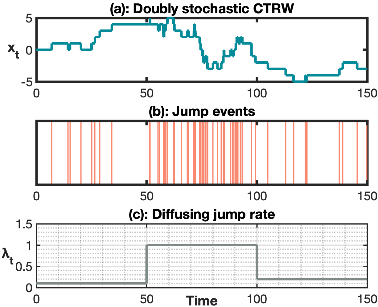
Figure 1: The doubly stochastic CTRW has three layers of randomness. The fluctuating jump rate $\lambda_{t}$ in panel (c) gives the probability $\lambda_{t}dt$ for a jump to occur in the time interval $\left[t,t+dt\right]$. When a jump event occurs, bar-coded in panel (b), the random walker draws a random step and jumps to a new position as shown in panel (a). Here, we illustrate this general modeling framework using a jump rate $\lambda_{t}$ that is redrawn, every $\tau_{r}=50$ units of time, from an exponential distribution with unit mean. In this example, jumps are assumed symmetric, with equal probability to make a right/left step ($\pm 1$). The resulting process exhibits periods of low and high activity, which give rise to deviations from Gaussian diffusion as observed in heterogeneous environments.

Diffusion can be seen as a continuum limit of a large class of random walk processes that occur on the microscopic scale. Yet, a general description of random walks with “diffusing diffusivity” is currently missing from the physics literature. To bridge this gap, we introduce a new modelling framework that sets the foundations for the study of the diffusing diffusivity phenomenology from a random walks perspective. We start from the widely applied continuous time random walk (CTRW) Montroll and Weiss (1965); Kutner and Masoliver (2017); Shlesinger (2017); Klafter and Sokolov (2011), where the walker jumps instantaneously from one position to another following a waiting period. In its simplest form, which gives rise to normal diffusion, waiting times in the CTRW are taken from an exponential distribution that is characterized by a constant jump rate $\lambda$. To introduce the equivalent of a diffusing diffusivity, we instead consider a diffusing jump rate $\lambda_{t}$ Cox (1955); Eliazar and Klafter (2005), such that the probability to make a jump during the time interval $[t,t+dt]$ is given by $\lambda_{t}dt$. This results in a doubly stochastic version of the continuous time random walk. Next, we show that this newly added layer of randomness gives rise to a rich phenomenology which captures, inter alia, both regular and anomalous diffusion. The analysis brought below will be focused on transport and first-passage properties, leaving the correlation structure of the process to future study.

Doubly stochastic continuous time random walk (DSCTRW).—The DSCTRW is schematised in Fig. 1. A random walker takes steps at random times which are determined by a Poisson process whose jump rate $\lambda_{t}$ is itself a random function of time. This doubly stochastic Poisson process is also known as a Cox process Cox (1955). When a jump event occurs, the random walker takes a step $X$ from a distribution whose characteristic function is $\hat{\phi}\left(k\right)=\langle e^{ikX}\rangle$. We note that in actuarial science an equivalent model, the doubly stochastic compound Poisson process, has been studied Bouzas et al. (2004); Peters et al. (2011); Léveillé and Hamel (2018). Also, the DSCTRW should not be confused with the noisy continuous time random walk Jeon et al. (2013) which is a different model.

The random walker’s displacement is determined by $P(x,t)$, the probability to find it in position $x$ at time $t$. To compute this probability, let us first assume a given path for the jump rate process $\lambda_{t}$. The resulting jump process is then a time inhomogeneous Poisson process, and therefore the number of steps made until time $t$ will be given by the Poisson distribution with mean $\Lambda_{t}=\int_{0}^{t}\lambda_{t^{\prime}}\text{d}t^{\prime}$ Kingman (1992); Gallager (2013). Letting $\chi_{n}(t)$ denote the probability that the random walker made exactly $n$ steps until time $t$ we thus have $\chi_{n}(t)=\frac{\Lambda_{t}^{n}}{n!}e^{-\Lambda_{t}}$. The Fourier transform of the probability distribution of the displacement, conditioned on a given path of the diffusing jump rate, reads

$$\hat{P}\left(k,t|\lambda_{t}\right)=\sum_{n=0}^{+\infty}\chi_{n}(t)\hat{\phi}(k)^{n}=e^{-(1-\hat{\phi}(k))\Lambda_{t}}.$$ (1)

Note, that this distribution only depends on the diffusing jump rate $\lambda_{t}$ through its time integral $\Lambda_{t}$. Averaging Eq. (1) with respect to the distribution of $\Lambda_{t}$, whose density we denote by $f(\Lambda_{t})$, we obtain

$$\hat{P}(k,t)=\tilde{\Lambda}_{t}(1-\hat{\phi}(k)),$$ (2)

where $\tilde{\Lambda}_{t}(1-\hat{\phi}(k))=\int_{0}^{\infty}e^{-[1-\hat{\phi}(k)]\Lambda_{t}}f(\Lambda_{t})\text{d}\Lambda_{t}$ is the Laplace transform of the integrated diffusing jump rate $\Lambda_{t}$ evaluated at $1-\hat{\phi}(k)$. Equation (2) is the DSCTRW analog of the Montroll-Weiss formula. We emphasize its generality, and that it holds for both stochastic and deterministic paths of $\lambda_{t}$.

Long-time behaviour.— Starting from Eq. (2), we can understand both the short and long time behavior of the DSCTRW. Specifically, under mild assumptions, the long-time behavior is universally Gaussian. To show this, we need the following assumptions: (i) the mean and variance of the step distribution are finite; and (ii) the integrated jump rate has the following long-time asymptotics: $\Lambda_{t}=\int_{0}^{t}\lambda_{t^{\prime}}\text{d}t^{\prime}\simeq\overline{\lambda}t+\zeta_{t}$, where $\overline{\lambda}$ is the long time average of the fluctuating jump rate and where $\zeta_{t}$ is Gaussian with $\langle\zeta_{t}\rangle=0$ and $\langle\zeta^{2}_{t}\rangle=o(t^{2})$. In particular, note that this condition holds for the typical case, $\langle\zeta^{2}_{t}\rangle\sim t$, that arises (due to the central limit theorem) for a fluctuating jump rate that has a finite correlation time and a steady-state distribution with a finite mean and variance. Under these assumptions, the Fourier transform of the scaled displacement converges to $\langle e^{ik\frac{x_{t}-\bar{\lambda}\langle X\rangle t}{\sigma(x_{t})}}\rangle\to e^{-\frac{k^{2}}{2}}$ Sup , which is the Fourier transform of the standard normal. This result is analogous to the long time asymptotics that is obtained using the diffusing diffusivity approach.

The Gaussian limit above is universal given the aforementioned assumptions. Yet, we note that these can be broken in several different ways. For example, akin to scaled Brownian motion  Safdari et al. (2015); Lim and Muniandy (2002); Jeon et al. (2014); He et al. (2008), one can think of cases where $\langle\lambda_{t}\rangle\propto\lambda t^{\alpha-1}$. These give $\langle\Lambda_{t}\rangle\propto\lambda t^{\alpha}$, which in turn yields sub-diffusion for $\alpha<1$ and super-diffusion for $\alpha>1$. However, unlike scaled Brownian motion, the DSCTRW also allows one to treat processes where the mean and/or variance of the step size diverge. Diverging moments of the step distribution prevent moment expansion of $\hat{\phi}(k)$ and yield, in the spirit of the generalized central limit theorem Lévy (1924); Klafter and Sokolov (2011), $\alpha$-stable Lévy asymptotics for the displacement. We illustrate this by taking steps from the Cauchy distribution, which returns a Cauchy distribution at long times (Fig. S1 in Sup ). A different way in which stable distributions may arise is when the jump rate has a steady-state with an infinite mean or variance. Such situations give rise to stable distributions for $\Lambda_{t}$, and the position distribution can then be computed via Eq. (2). The above-mentioned scenarios illustrate the richness of DSCTRW and highlight that this model can describe scenarios that fall outside the scope of the diffusing diffusivity model.

Short-time behaviour.—Contrary to long times, the short time displacement distribution is not universal and its shape depends on the steady-state distribution of the diffusing jump rate. Assuming the latter exists, we consider a case where the diffusing jump rate has been evolving for a very long time prior to the start of the experiment, such that it has converged to its steady-state. In the short time limit $t\ll\tau_{r}$, with $\tau_{r}$ being the typical relaxation time of the diffusing jump rate process, the integrated rate behaves like $\Lambda_{t}=\int_{0}^{t}\lambda_{t^{\prime}}\text{d}t^{\prime}\simeq t\lambda_{e}$ with $\lambda_{e}$ drawn from the steady-state distribution whose Laplace transform we denote by $\tilde{\lambda}_{e}(s)=\langle e^{-s\lambda_{e}}\rangle$.

Under these assumptions, the Laplace transform of the integrated rate can be expressed using the Laplace transform of the jump rate, $\tilde{\Lambda}_{t}(s)=\tilde{\lambda}_{e}(ts)$ and together with Eq. (2) we have

$$\hat{P}(k,t)=\tilde{\lambda}_{e}\left(t(1-\hat{\phi}(k))\right).$$ (3)

Thus if we study the tail of this distribution in the case of a symmetric walk, we obtain $\hat{P}(k,t)\simeq\tilde{\lambda}_{e}(tk^{2}\langle X^{2}\rangle/2)$, which is a symmetric version of the rate probability distribution, that has no reason of being universal. For example, if $\lambda_{e}$ is exponentially distributed with mean $\overline{\lambda}$ – which is the case for a jump rate process that is diffusing on $\mathbb{R}_{+}$ and with a negative drift pointing towards the origin – we obtain $\hat{P}(k,t)\simeq\frac{1}{1+\overline{\lambda}tk^{2}\langle X^{2}\rangle/2}$ which is the Fourier transform of the Laplace distribution, also known as the bi-exponential. The probability distribution is then given by $P(x,t)=\frac{1}{2\sigma_{t}}e^{-\frac{|x|}{\sigma_{t}}},$ with $\sigma_{t}=\sqrt{\overline{\lambda}t\langle X^{2}\rangle/2}$. This result is not universal, but noteworthy since the central limit theorem asserts that drift-diffusion often provides an excellent approximation to a host of biased random walk processes that may govern the fluctuating jump rate. This could, perhaps, explain the prevalence of exponential tails observed experimentally at short times. For an alternative explanation see Refs. Barkai and Burov (2020); Wang et al. (2020b).

Moments.—Moments in the DSCTRW can be computed by taking derivatives of Eq. (2): $\langle x_{t}^{n}\rangle=\lim_{k\to 0}(-i)^{n}\frac{\text{d}^{n}\hat{P}(k,t)}{\text{d}k^{n}}$. Specifically, we find that while the displacement probability distribution displays a non-Gaussian to Gaussian transition, the MSD of an unbiased walk is linear at all times $\langle x_{t}^{2}\rangle=\langle X^{2}\rangle\langle\Lambda_{t}\rangle=\langle X^{2}\rangle\overline{\lambda}t$  Sup , provided $\lambda_{t}$ starts equilibrated and has a finite mean. More generally, the time dependence of the MSD is completely determined by the first moment of the integrated diffusing jump rate process and the second moment of the jump. The fourth moment of a symmetric DSCTRW is given by $\langle x_{t}^{4}\rangle=\langle X^{4}\rangle\langle\Lambda_{t}\rangle+3\langle X^{2}\rangle^{2}\langle\Lambda_{t}^{2}\rangle$ Sup .

When bias is introduced to the random walk, the variance in position is given by $\sigma^{2}(x_{t})=\langle X^{2}\rangle\langle\Lambda_{t}\rangle+\langle X\rangle^{2}(\langle\Lambda_{t}^{2}\rangle-\langle\Lambda_{t}\rangle^{2})$ Sup . Thus, when the integrated rate is stochastic, its variance does not vanish, resulting in additional dispersion. We illustrated this for a biased version of the toy model in Fig. 1. There the mean and variance of the integrated jump rate are both linear in time, which leads to an apparent diffusion coefficient that can be significantly larger than in the absence of bias (Fig. S2 in SM Sup ). This enhanced dispersion, can be traced to the inherent coupling between drift and diffusion in the DSCTRW. Notably, the effect is absent from the diffusing diffusivity model, where drift and diffusion are completely decoupled.

An exactly solvable DSCTRW.— To further illustrate the DSCTRW, we return to the model illustrated in Fig. 1. There the diffusing jump rate is drawn every $\tau_{r}$ from an exponential distribution with mean jump rate $\bar{\lambda}=1$. The resulting jump rate is piece-wise constant, i.e., changes abruptly when a new time window starts. This can be seen as a simplified picture of more complicated diffusing jump rate processes whose autocorrelation time, $\tau_{r}$, is finite.

To get the propagator using Eq. (2), we compute the Laplace transform of the integrated jump rate, which in our model is a sum of independent random variables $\Lambda_{t}=\sum_{i=1}^{n_{\tau_{r}}}\lambda_{i}\tau_{r}+\lambda_{n_{\tau_{r}+1}}\delta_{t}$ with $n_{\tau_{r}}=\left\lfloor\frac{t}{\tau_{r}}\right\rfloor$ and $\delta_{t}=t-n_{\tau_{r}}\tau_{r}$. Therefore the Laplace transform, in Eq. (2) is a product of Laplace transforms of exponentially distributed random variables

$$\hat{P}(k,t)=\tilde{\lambda}_{e}\left((1-\hat{\phi}(k))\tau_{r}\right)^{n_{\tau_{r}}}\tilde{\lambda}_{e}\left((1-\hat{\phi}(k))\delta_{t}\right),$$ (4)

with $\tilde{\lambda}_{e}(s)=1/(1+\bar{\lambda}s)$. Taking the walk to be simple symmetric, we have $\phi(k)=\cos(k)$, and a Laplace to Gaussian transition is observed when going from the short-time limit $t\ll\tau_{r}$ to the long-time limit $t\gg\tau_{r}$ (Fig. 2).

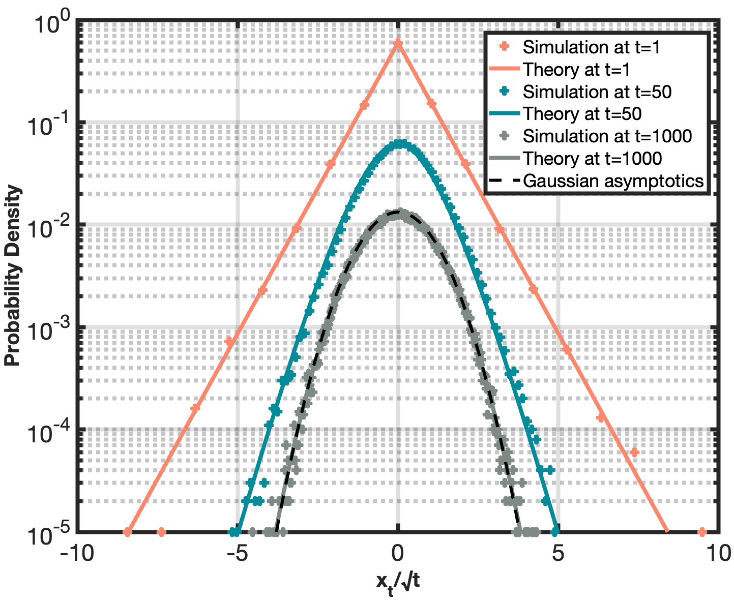
Figure 2: Displacement probability distributions for the DSCTRW illustrated in Fig. 1. Circles come from simulations and bold lines give analytical results obtained by inverting the Fourier transform in Eq. (4). Here, the mean jump rate was set to unity and its relaxation time to $\tau_{r}=10$. The distributions are plotted for three different times: $t=0.1\tau_{r}$ (orange) that exhibits a Laplace distribution, $t=5\tau_{r}$ (cyan) for which we see the beginning of a transition towards the Gaussian distribution, and $t=100\tau_{r}$ (gray) where the displacement distribution has converged to the Gaussian.

First passage statistics.—The random time at which a stochastic process reaches a certain threshold, e.g. the encounter time of two molecules or the time a stock hits a certain price, can trigger a series of events. Thus, understanding the properties of first passage times is key to the explanation of many phenomena in statistical physics, chemistry, and finance Redner (2001); Metzler et al. (2014); Bray et al. (2013). To show how first-passage problems are solved in the context of the DSCTRW, we continue with the model illustrated in Fig. 1 and derive its first exit time from an interval. This exit time exhibits interesting phenomenology due to the competition between different timescales.

To obtain the exit time, we apply two simple steps: we first calculate the propagator conditioned on the number of steps taken, and then translate steps to time by summing over the corresponding probabilities $\chi_{n}(t)$. The propagator of the simple symmetric random walk inside an interval $[0,L]$ with absorbing boundaries is given by Feller (1991)

$$P(x,n|x_{0})=\frac{2}{L}\sum_{p=0}^{L}\eta_{p}^{n}\sin(\nu_{p}x_{0})\sin(\nu_{p}x),$$ (5)

where $x_{0}$ is the initial position, $\nu_{p}=\frac{p\pi}{L}$ and $\eta_{p}=\cos{\nu_{p}}$. In the following we set $u_{p}(x_{0},x)=\sin(\nu_{p}x_{0})\sin(\nu_{p}x)$. Translating steps to time, averaging over $\Lambda_{t}$, and summing over all lattice sites inside the interval, we obtain the survival probability

$$S(t|x_{0})=\frac{2}{L}\sum_{x=1}^{L-1}\sum_{p=0}^{L}u_{p}(x_{0},x)\tilde{\Lambda}_{t}(1-\eta_{p}),$$ (6)

where $\tilde{\Lambda}_{t}$ which previously appeared in Eq. (2) should now be evaluated at $1-\eta_{p}$ instead of $1-\hat{\phi}(k)$. Taking the negative time derivative of $S(t|x_{0})$, we obtain the probability density of the exit time

$$f(t|x_{0})=\frac{2\bar{\lambda}}{L}\sum_{x=1}^{L-1}\sum_{p=0}^{L}\frac{u_{p}(x_{0},x)(1-\eta_{p})\tilde{\Lambda}_{t}(1-\eta_{p})}{1+(1-\eta_{p})\delta_{t}\bar{\lambda}}.$$ (7)

Analyzing the density in Eq. (7) right before and just after integer multiples of $\tau_{r}$, we analytically show that it experiences jumps whose magnitude increases with $\tau_{r}$ Sup . This feature is a manifestation of the sharp transitions experienced by the diffusing jump rate in our model (Fig. 1c). Indeed, particles that initially drew a smaller than average jump rate have a higher probability to survive simply by virtue of moving less. As a result, the system becomes enriched with such particles, until a new jump rate is redrawn at $t=\tau_{r}$. This leads to a jumps in the first-exit density, which come from slowly moving particles that become faster moving and perish.

The jump rate relaxation time, $\tau_{r}$, also has a profound impact on the mean first exit time (MFET) from the interval, which we obtain by averaging over the density in Eq. (7). Results are given in Fig. 3, where we distinguish between two limiting behaviours. When relaxation times are fast, jump rate fluctuations play a lesser role as they are averaged over. In this limit, the jump rate can be seen as if it was fixed and equal to the mean jump rate $\overline{\lambda}$. The MFET can then be approximated as $\simeq(L-x_{0})x_{0}/\overline{\lambda}$, which is the MFET of a simple CTRW with a fixed jump rate $\overline{\lambda}$. Situation is different for slow relaxation times $\tau_{r}\gg(L-x_{0})x_{0}/\overline{\lambda}$. In this case, a typical particle is “stuck” with its initially drawn jump rate until it leaves the interval. The MFET can then be approximated by averaging $(L-x_{0})x_{0}/\lambda$ over the initial distribution of the jump rate $\lambda$ (here assumed equivalent to the steady-state distribution). Doing so for an exponential distribution of jump rates leads to a logarithmic divergence, which we regularize by noting that the relaxation rate, $\tau_{r}^{-1}$, serves a lower cutoff for the integration. Indeed, very slow particles that do not leave the interval by the relaxation time, will consequently draw a new jump rate. More generally we find that the asymptotic dependence of the MFET on $\tau_{r}$ depends on the small rate asymptotics of steady-state distribution of the jump rate Sup .

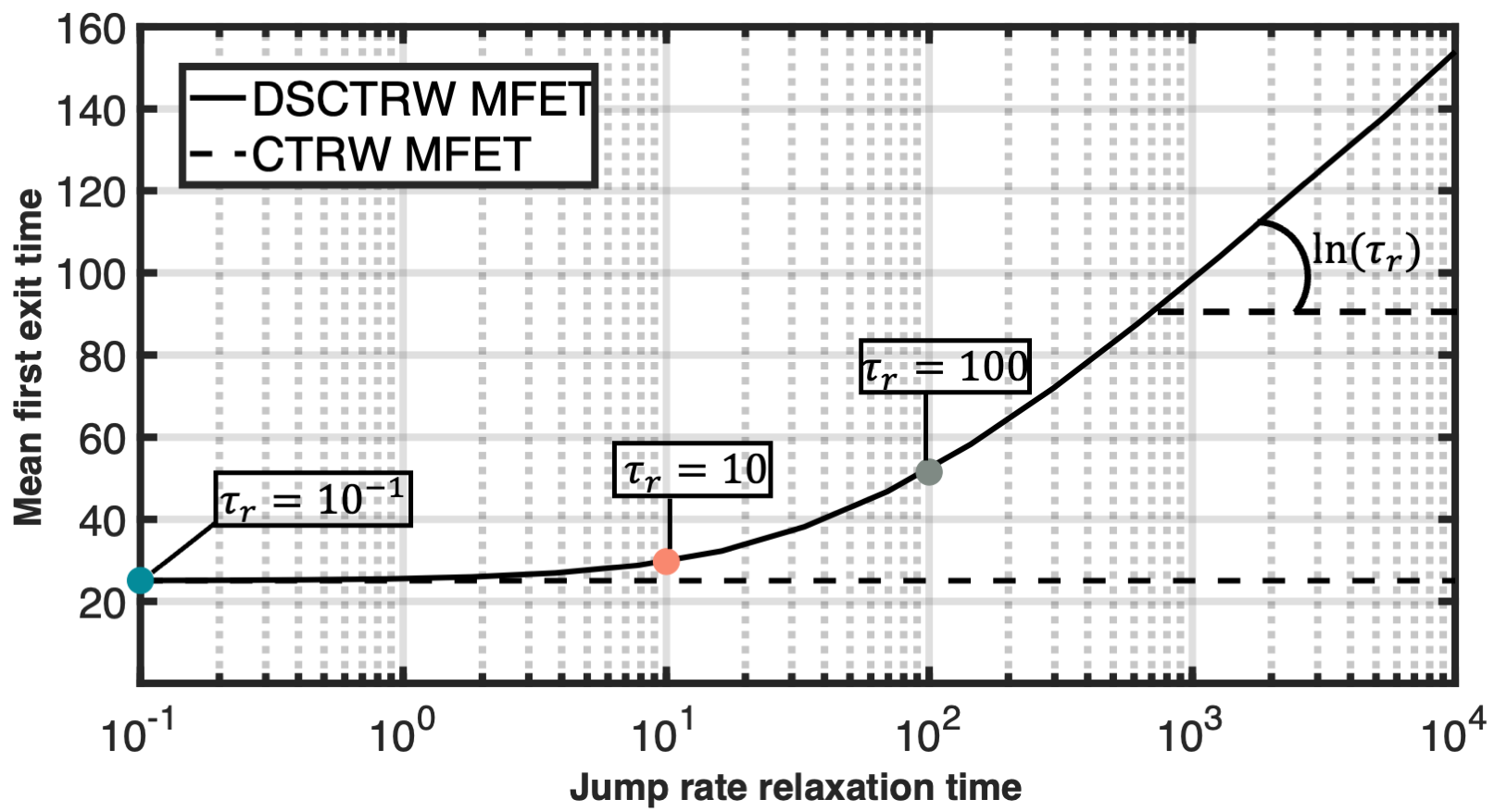
Figure 3: Mean first exit time (MFET) from the interval $\left[0,10\right]$, starting at $x_{0}=5$, for the DSCTRW illustrated in Fig. 1. For fast jump rate relaxation (small $\tau_{r}$), we recover the MFET of a simple CTRW (dashed line) with a fixed jump rate corresponding to the mean jump rate, $\overline{\lambda}=1$, of the DSCTRW. In the other extreme, i.e., for slow relaxation times (large $\tau_{r}$), the MFET scales as $\sim\ln(\tau_{r})$. The bold line is plotted by averaging over Eq. (7) and circles denote MFETs that correspond to the distributions in Fig. S3.

We note that the first-passage results obtained above can be generalized for many other geometries and boundary conditions. This can be done whenever the propagator in real, or Fourier space, admits a standard eigenmode expansion of the form which appears in Eq. (5). Crucially, when terms in the series are proportional to $\eta_{p}^{n}$ , one can easily translate steps to time by summing over the corresponding probabilities $\chi_{n}(t)$ and taking expectations. For additional examples that can be solved in a similar fashion see Giuggioli (2020), which gives exact results for propagators of random walks in confined geometries.

Conclusions.—In this letter, we introduced a doubly stochastic version of the renowned CTRW. The model allows for a general description of a random walk which is driven by a time dependent jump rate that fluctuates randomly. Despite this added layer of complexity, the model remains fully tractable and we obtained a general formula for the displacement probability distribution. A rich phenomenology emerged from the analysis, asserting that the doubly stochastic continuous time random walk can be used to describe not only super, sub, and normal diffusion, but also the Brownian yet non-Gaussian diffusion that has recently been observed in various systems. The tractability of the model further lends itself to the computation of first-passage times which—similar to the displacement distribution—display striking transitions as a function of the jump rate relaxation time. The random walk approach developed herein complements the diffusing diffusivity approach that was developed for Brownian motion, and further extends it by allowing for unlimited freedom in the interplay between the distribution of jumps and the properties of the fluctuating jump rate.

Acknowledgments.—M.A. acknowledges discussions with Samuel Gelman, Ulysse Mizrahi and Bara Levit. S.R. acknowledges support from the Israel Science Foundation (grant No. 394/19). This project received funding from the European Research Council (ERC) under the European Union’s Horizon 2020 research and innovation program (Grant agreement No. 947731).

References

- Havlin and Ben-Avraham (1987) S. Havlin and D. Ben-Avraham, Advances in physics 36, 695 (1987).
- Bouchaud and Georges (1990) J. P. Bouchaud and A. Georges, Physics reports 195, 127 (1990).
- Metzler and Klafter (2000) R. Metzler and J. Klafter, Physics reports 339, 1 (2000).
- Sokolov (2012) I. M. Sokolov, Soft Matter 8, 9043 (2012).
- Barkai et al. (2012) E. Barkai, Y. Garini, and R. Metzler, Phys. Today 65, 29 (2012).
- Wang et al. (2009) B. Wang, S. M. Anthony, S. C. Bae, and S. Granick, Proceedings of the National Academy of Sciences 106, 15160 (2009).
- Wang et al. (2012) B. Wang, J. Kuo, S. C. Bae, and S. Granick, Nature materials 11, 481 (2012).
- Kim et al. (2013) J. Kim, C. Kim, and B. J. Sung, Physical review letters 110, 047801 (2013).
- Guan et al. (2014) J. Guan, B. Wang, and S. Granick, ACS nano 8, 3331 (2014).
- Acharya et al. (2017) S. Acharya, U. K. Nandi, and S. Maitra Bhattacharyya, The Journal of Chemical Physics 146, 134504 (2017).
- Chakraborty et al. (2019) I. Chakraborty, G. Rahamim, R. Avinery, Y. Roichman, and R. Beck, Nano letters 19, 6524 (2019).
- Chakraborty and Roichman (2020) I. Chakraborty and Y. Roichman, Physical Review Research 2, 022020 (2020).
- Beck (2001) C. Beck, Physical Review Letters 87, 180601 (2001).
- Beck and Cohen (2003) C. Beck and E. G. Cohen, Physica A: Statistical mechanics and its applications 322, 267 (2003).
- Metzler (2020) R. Metzler, The European Physical Journal Special Topics 229, 711 (2020).
- Chubynsky and Slater (2014) M. V. Chubynsky and G. W. Slater, Physical review letters 113, 098302 (2014).
- Jain and Sebastian (2016) R. Jain and K. L. Sebastian, The Journal of Physical Chemistry B 120, 3988 (2016).
- Jain and Sebastian (2017) R. Jain and K. Sebastian, Journal of Chemical Sciences 129, 929 (2017).
- Tyagi and Cherayil (2017) N. Tyagi and B. J. Cherayil, The Journal of Physical Chemistry B 121, 7204 (2017).
- Chechkin et al. (2017) A. V. Chechkin, F. Seno, R. Metzler, and I. M. Sokolov, Physical Review X 7, 021002 (2017).
- Sposini et al. (2018) V. Sposini, A. V. Chechkin, F. Seno, G. Pagnini, and R. Metzler, New Journal of Physics 20, 043044 (2018).
- Lanoiselée and Grebenkov (2018) Y. Lanoiselée and D. S. Grebenkov, Journal of Physics A: Mathematical and Theoretical 51, 145602 (2018).
- Lanoiselée et al. (2018) Y. Lanoiselée, N. Moutal, and D. S. Grebenkov, Nature communications 9, 1 (2018).
- Thapa et al. (2018) S. Thapa, M. A. Lomholt, J. Krog, A. G. Cherstvy, and R. Metzler, Physical Chemistry Chemical Physics 20, 29018 (2018).
- Wang et al. (2020a) W. Wang, F. Seno, I. M. Sokolov, A. V. Chechkin, and R. Metzler, New Journal of Physics 22, 083041 (2020a).
- Nampoothiri et al. (2021) S. Nampoothiri, E. Orlandini, F. Seno, and F. Baldovin, Physical Review E 104, L062501 (2021).
- Pacheco-Pozo and Sokolov (2021) A. Pacheco-Pozo and I. M. Sokolov, Physical Review Letters 127, 120601 (2021).
- Nampoothiri et al. (2022) S. Nampoothiri, E. Orlandini, F. Seno, and F. Baldovin, New Journal of Physics 24, 023003 (2022).
- Marcone et al. (2022) B. Marcone, S. Nampoothiri, E. Orlandini, F. Seno, and F. Baldovin, Journal of Physics A: Mathematical and Theoretical 55, 354003 (2022).
- Alexandre et al. (2022) A. Alexandre, M. Lavaud, N. Fares, E. Millan, Y. Louyer, T. Salez, T. Guérin, D. S. Dean, et al., arXiv preprint arXiv:2207.01880 (2022).
- Dragulescu and Yakovenko (2002) A. A. Dragulescu and V. M. Yakovenko, Quantitative finance 2, 443 (2002).
- Silva et al. (2004) A. C. Silva, R. E. Prange, and V. M. Yakovenko, Physica A: Statistical Mechanics and its Applications 344, 227 (2004).
- Bouchaud et al. (2003) J.-P. Bouchaud, M. Potters, et al., Theory of financial risk and derivative pricing: from statistical physics to risk management (Cambridge university press, 2003).
- Montroll and Weiss (1965) E. W. Montroll and G. H. Weiss, Journal of Mathematical Physics 6, 167 (1965).
- Kutner and Masoliver (2017) R. Kutner and J. Masoliver, The European Physical Journal B 90, 1 (2017).
- Shlesinger (2017) M. F. Shlesinger, The European Physical Journal B 90, 1 (2017).
- Klafter and Sokolov (2011) J. Klafter and I. M. Sokolov, First steps in random walks: from tools to applications (OUP Oxford, 2011).
- Cox (1955) D. R. Cox, Journal of the Royal Statistical Society: Series B (Methodological) 17, 129 (1955).
- Eliazar and Klafter (2005) I. Eliazar and J. Klafter, Journal of statistical physics 120, 587 (2005).
- Bouzas et al. (2004) P. Bouzas, M. Valderrama, and A. Aguilera, Applied Mathematical Modelling 28, 769 (2004).
- Peters et al. (2011) G. W. Peters, P. V. Shevchenko, M. Young, and W. Yip, Insurance: Mathematics and Economics 49, 565 (2011).
- Léveillé and Hamel (2018) G. Léveillé and E. Hamel, Methodology and Computing in Applied Probability 20, 353 (2018).
- Jeon et al. (2013) J.-H. Jeon, E. Barkai, and R. Metzler, The Journal of Chemical Physics 139 (2013).
- Kingman (1992) J. F. C. Kingman, Poisson processes, Vol. 3 (Clarendon Press, 1992).
- Gallager (2013) R. G. Gallager, Stochastic processes: theory for applications (Cambridge University Press, 2013).
- (46) See Supplemental Material .
- Safdari et al. (2015) H. Safdari, A. V. Chechkin, G. R. Jafari, and R. Metzler, Physical Review E 91, 042107 (2015).
- Lim and Muniandy (2002) S. C. Lim and S. V. Muniandy, Physical Review E 66, 021114 (2002).
- Jeon et al. (2014) J.-H. Jeon, A. V. Chechkin, and R. Metzler, Physical Chemistry Chemical Physics 16, 15811 (2014).
- He et al. (2008) Y. He, S. Burov, R. Metzler, and E. Barkai, Physical Review Letters 101, 058101 (2008).
- Lévy (1924) P. Lévy, Bulletin de la Société mathématique de France 52, 49 (1924).
- Barkai and Burov (2020) E. Barkai and S. Burov, Physical review letters 124, 060603 (2020).
- Wang et al. (2020b) W. Wang, E. Barkai, and S. Burov, Entropy 22, 697 (2020b).
- Redner (2001) S. Redner, A guide to first-passage processes (Cambridge university press, 2001).
- Metzler et al. (2014) R. Metzler, S. Redner, and G. Oshanin, First-passage phenomena and their applications, Vol. 35 (World Scientific, 2014).
- Bray et al. (2013) A. J. Bray, S. N. Majumdar, and G. Schehr, Advances in Physics 62, 225 (2013).
- Feller (1991) W. Feller, An introduction to probability theory and its applications, Volume 1 (John Wiley & Sons, 1991).
- Giuggioli (2020) L. Giuggioli, Physical Review X 10, 021045 (2020).