Spatial Joint Models through Bayesian Structured Piece-wise Additive Joint Modelling for Longitudinal and Time-to-Event Data

Abstract

Joint models for longitudinal and time-to-event data have seen many developments in recent years. Though spatial joint models are still rare and the traditional proportional hazards formulation of the time-to-event part of the model is accompanied by computational challenges. We propose a joint model with a piece-wise exponential formulation of the hazard using the counting process representation of a hazard and structured additive predictors able to estimate (non-)linear, spatial and random effects. Its capabilities are assessed in a simulation study comparing our approach to an established one and highlighted by an example on physical functioning after cardiovascular events from the German Ageing Survey. The Structured Piece-wise Additive Joint Model yielded good estimation performance, also and especially in spatial effects, while being double as fast as the chosen benchmark approach and performing stable in imbalanced data setting with few events.

Keywords Bayesian statistics  $\cdot$ joint models  $\cdot$ piecewise additive mixed models  $\cdot$ piecewise exponential

1 Introduction

Biometrical studies often capture time-to-event and longitudinal data on the same topic simultaneously. Frequently used examples are the count of CD4 lymphocytes in HIV-positive patients and their time till onset of AIDS (Faucett and Thomas 1996; Wulfsohn and Tsiatis 1997; Rizopoulos 2011) or the level of serum bilirubin and other liver biomarkers in primary biliary cirrhosis patients and time to death (Crowther, Abrams, and Lambert 2013; Hickey et al. 2018). Other examples include PSA cancer marker and progression to recurrence of prostate cancer (Jacqmin-Gadda et al. 2010), autoantibody titers in children preceding the onset of Type 1 diabetes (Köhler, Beyerlein, et al. 2017) or physical functioning after a cardiovascular event and death (Rappl, Mayr, and Waldmann 2022). Separate analysis of these longitudinal and time-to-event outcomes leads to biased estimates and to avoid this both should be modelled jointly. These joint models consist of two submodels: A longitudinal submodel and a survival submodel with both being linked through an association parameter.
While Wulfsohn and Tsiatis (1997) and Henderson, Diggle, and Dobson (2000) proposed to maximize the likelihood of a joint model via an Expectation-Maximization (EM) algorithm, Faucett and Thomas (1996) used a Bayesian Gibbs-sampling approach. In recent years advances have been made into statistical boosting (Waldmann et al. 2017; Griesbach, Groll, and Bergherr 2021). Software is available for all three estimation approaches across various statistical computation platforms, of which especially R hosts a number of well-established packages such as JM (Rizopoulos 2010), JMbayes (Rizopoulos 2016), joineRML (Hickey et al. 2018) and bamlss (Umlauf et al. 2021). Comparisons of selections of available software can be found in Yuen and Mackinnon (2016) and Rappl, Mayr, and Waldmann (2022).
Traditionally the longitudinal submodel of a joint model is a linear mixed model (LMM) and the time-to-event submodel is a proportional hazards (PH) model, though other variants are possible. Depending on the scaling of the longitudinal outcome a generalized linear mixed model (GLMM) (Faucett, Schenker, and Elashoff 1998; Rizopoulos et al. 2008; Viviani, Alfó, and Rizopoulos 2014) or quantile regression model (Y. Huang and Chen 2016; Zhang et al. 2019) might be better suited. An alternative to the PH-models in the time-to-event submodel are accelerated failure time models (Tseng, Hsieh, and Wang 2005; Y. Huang and Chen 2016) and in certain data situations competing risks models are best suited (X. Huang et al. 2011; Andrinopoulou et al. 2014; Blanche et al. 2015). Also models with multivariate longitudinal outcomes are in use (Lin, McCulloch, and Mayne 2002; Rizopoulos and Ghosh 2011; Mauff et al. 2020) as are location-scale models (Barrett et al. 2019). Köhler, Umlauf, et al. (2017) expanded joint models to structured additive joint models with possibly smooth random effects and established non-linear association structures (2018) both via a Bayesian flexible tensor-product approach using Newton-Raphson procedures and derivative-based Metropolis-Hastings sampling. A good historic overview on joint models can be found in Tsiatis and Davidian (2004), while Alsefri et al. (2020) give a concise summary of recent developments in Bayesian joint models in particular.
Still joint models with a spatial component are rare. Martins, Silva, and Andreozzi (2016) and Martins, Silva, and Andreozzi (2017) have described estimation of a Bayesian joint model with a spatial effect and a Weibull baseline hazard using OpenBUGS and WinBUGS respectively. The above mentioned Bayesian tensor-product approach by Köhler, Umlauf, et al. (2017) implemented in the R package bamlss also has the capability of estimating spatial joint models. In terms of model formulation both methods have in common that they use a PH-model for the survival submodel. However, assuming a parametric baseline hazard such as a Weibull hazard can be restrictive and derivative-based Metropolis-Hastings algorithms are computationally expensive as well as may prove sensitive towards data with few events.
Therefore, in this paper we propose a Bayesian joint model with a structured additive LMM for the longitudinal outcome, but exchange the time-to-event submodel for a piece-wise additive mixed model (PAMM). The latter has been suggested by Bender, Groll, and Scheipl (2018) for modelling survival times based on the proportionality of a time-to-event process with a Poisson-distributed count process (Friedman 1982) thus expanding the available options for time-to-event models (e.g. accelerated failure times, competing risk). This formulation allows for estimation of the baseline hazard without any assumptions about its distributional form and is similarly flexible to the Köhler, Umlauf, et al. (2017) model with respect to the inclusion of (non-)linear, spatial and random effects. At the same time, it reduces runtimes by about 50% (compared to an established method) and has proven stable in imbalanced data settings with few events.
The rest of the paper is structured as follows: In the next section, the methodology of piece-wise additive joint models is described in more detail and our extension of the concept is explained. In section three the results of a simulation study comparing our approach to an established one to proof the feasibility of the model formulation, its ability to estimate spatial effects and its runtime performance. We then apply this method to an example of physical functioning from the German Aging Survey. Section five concludes with some final remarks and further technical details can be found in the Appendix.

2 Methods

2.1 Theoretical background

In its original form the Joint Model assumes a linear mixed model (LMM) for the longitudinal outcome and a proportional hazards model (PH) for the time-to-event outcome (Wulfsohn and Tsiatis 1997; Faucett and Thomas 1996; Henderson, Diggle, and Dobson 2000).
Let $\boldsymbol{y}$ denote the vector of longitudinal outcomes across all individuals $i=\{1,\dots,n\}$ and observations times points $t$. Further, let $\boldsymbol{\lambda}(t)$ be the vector of individual specific risks to experience an event at time $t$ proportional to the baseline hazard $\lambda_{0}(t)$ and based on the observed event or censoring times $\boldsymbol{T}$ and event indicator $\boldsymbol{\delta}$. Then in its most generic variant the original joint model takes the form

$$\boldsymbol{y}(t) =\boldsymbol{\eta}_{\text{l}}(t)+\boldsymbol{\eta}_{\text{ls}}(t)+\varepsilon,\quad\varepsilon\sim\text{N}(0,\sigma^{2}\boldsymbol{I})$$ (1)

$$\boldsymbol{\lambda}(t) =\lambda_{0}(t)\exp\{\boldsymbol{\eta}_{\text{s}}+\alpha\boldsymbol{\eta}_{\text{ls}}(t)\},$$ (2)

where $\boldsymbol{\eta}_{\text{s}}$ and $\boldsymbol{\eta}_{\text{l}}$ are survival and respectively longitudinal submodel specific predictors and $\boldsymbol{\eta}_{\text{ls}}$ is the shared predictor, via which both model parts are connected. The parameter $\alpha$ quantifies the association between the longitudinal and the time-to-event outcome. In the following, the addendum $\cdot(t)$ to denote time-varying predictors is dropped for ease of notation, since the subsequent concepts can be applied to time-varying and -constant predictors alike. Also note that, while it is theoretically possible to estimate time-varying survival predictors $\boldsymbol{\eta}_{\text{s}}(t)$, the time-varying covariates included in that predictor may be prone to measurement error and it is therefore in most cases better to model them jointly.
The predictors $\boldsymbol{\eta}_{\cdot}$ are additive and may include (non-)linear, geographical or random effects of potentially time-varying covariates $\boldsymbol{x}_{k}(t)$, i.e. $\boldsymbol{\eta}_{\cdot}=\sum_{k=1}^{p_{\cdot}}f_{k}(\boldsymbol{x}_{k}(t))$, where $f_{k}$ is a function representing the respective effect and $p_{\cdot}$ denotes the predictor specific number of covariates. Restrictions apply to random effects, which need to be part of the shared predictor $\boldsymbol{\eta}_{\text{ls}}$, and geographical effects, of which there can only be one in the model for identifiability reasons.
Reformulating predictor $\boldsymbol{\eta}_{\cdot}$ in matrix notation yields

$$\boldsymbol{\eta}_{\cdot}=\boldsymbol{Z}_{1}\boldsymbol{\gamma}_{1}+\cdots+\boldsymbol{Z}_{p_{\cdot}}\boldsymbol{\gamma}_{p_{\cdot}},$$ (3)

where $\boldsymbol{Z}_{k}$ is an effect appropriate design matrix and $\boldsymbol{\gamma}_{k}$ a vector of corresponding effect coefficients. For the Bayesian estimation of this model the generic prior for the coefficients $\boldsymbol{\gamma}_{k}$ is proportional to a normal distribution with zero mean, variance $\sigma_{\gamma_{k}}^{2}$ and penalty matrix $\boldsymbol{K}_{k}$

$$p\left(\boldsymbol{\gamma}_{k}\mid\sigma_{\gamma_{k}}^{2}\right)\propto\left(\sigma_{\gamma_{k}}^{2}\right)^{-\text{rk}(\boldsymbol{K}_{k})}\exp\left\{-\frac{1}{2\sigma_{\gamma_{k}}^{2}}\boldsymbol{\gamma}_{k}^{\prime}\boldsymbol{K}_{k}\boldsymbol{\gamma}_{k}\right\}.$$ (4)

For non-linear and spatial effects the penalty matrix $\boldsymbol{K}_{k}$ is rank deficient and as a result prior (4) is partially improper.
Linear effects. For a vector $\boldsymbol{\gamma}_{k}=(\gamma_{k_{1}},\dots,\gamma_{k_{J_{k}}})^{\prime}$ of $J_{k}$ linear fixed effects the penalty matrix $\boldsymbol{K}_{k}$ is an $J_{k}\times J_{k}$ identity matrix $\boldsymbol{I}_{J_{k}}$ reducing (4) to a $J_{k}$-variate normal distribution. An alternative is to set $p(\gamma_{k_{j}}\mid\cdot)\propto const\quad\forall j=1,\dots,J_{k}$. The corresponding design matrix $\boldsymbol{Z}_{k}$ is a matrix of covariates of order $n\times J_{k}$, where $n$ denotes the number of observations.
Random effects. In the case of joint models random effects appear in the shared predictor exclusively. Thus let $n$ be the number of individuals and $n_{i}$ be the number of observations per individual $i$, so that the total number of observations amounts to $N=\sum_{i=1}^{n}n_{i}$. Further, let $\boldsymbol{u}_{i}$ be a vector of observations (or $\boldsymbol{1}$ for random intercepts) of length $n_{i}$ specific to individual $i$. Then $\boldsymbol{Z}_{k}$ is a matrix of vectors $\boldsymbol{u}_{i}$ of order $N\times n$, i.e. $\boldsymbol{Z}_{k}=\text{diag}(\boldsymbol{u}_{1},\dots,\boldsymbol{u}_{n})$ and $\boldsymbol{\gamma}_{k}$ is a vector of random effects $b_{i}$ of length $n$, $\boldsymbol{\gamma}_{k}=(b_{1},\dots,b_{n})^{\prime}$. The penalty matrix $\boldsymbol{K}_{k}$ then is an $n\times n$ identity matrix $\boldsymbol{I}_{n}$.
Non-linear effects. Modelling non-linear effects follows the Bayesian P-spline approach with $\boldsymbol{Z}_{k}$ being a matrix of B-spline basis functions evaluated at observations $x_{i}(t)$. Then $\boldsymbol{\gamma}_{k}$ is a vector of corresponding basis coefficients. The common choice of prior for these basis coefficients is a first or second order random walk. This is achieved by setting the penalty matrix $\boldsymbol{K}_{k}$ equal to $\boldsymbol{D}^{\prime}\boldsymbol{D}$, i.e. $\boldsymbol{K}_{k}=\boldsymbol{D}^{\prime}\boldsymbol{D}$, where $\boldsymbol{D}$ is a matrix of first or second order differences.
Spatial effects. For spatial effects $\boldsymbol{Z}_{k}$ is assumed to be an $n\times S$ incidence matrix (potentially also $N\times S$, for spatio-temporal observations) with an entry of $1$ if observation $i\;\forall\;i=1,\dots,n$ originates from location $s\;\forall\;s=1,\dots,S$ with $S$ unique locations and $0$ otherwise. The corresponding coefficients $\boldsymbol{\gamma}_{k}$ follow a Markov random field (MRF) prior achieved via the penalty matrix $\boldsymbol{K}_{k}$. $\boldsymbol{K}_{k}$ is an adjacency matrix of order $S\times S$ with entries as the number of neighbours $|n(s)|$ only when locations $s$ and $r$ are neighbours ($s\sim r$) of the form

$$\boldsymbol{K}_{k}[s,r]=\begin{cases}-1&\text{if }s\neq r,s\sim r\\ 0&\text{if }s\neq r,s\not\sim r\\ |n(s)|&\text{if }s=r\end{cases}.$$

The variance parameters of the coefficient distributions $\sigma_{\gamma_{k}}^{2}$ as well as the model variance $\sigma_{\varepsilon}^{2}$ will a priori follow inverse gamma distributions, in particular

$$\sigma_{\gamma_{k}}^{2}\sim\text{IG}(a,b)\quad\text{and}$$

$$\sigma_{\varepsilon}^{2}\sim\text{IG}(a_{0},b_{0}).$$

2.2 The piecewise expontential representation of the time-to-event submodel

The idea behind a PH-model is that an individual’s hazard at time $t$ is determined by an individual specific deviation of an underlying baseline hazard $\lambda_{0}(t)$ at time $t$. In mathematical notation a generic PH-model looks similar to (2) and takes the form

$$\boldsymbol{\lambda}(t)=\lambda_{0}(t)\exp\{\boldsymbol{\eta}\},$$

where $\boldsymbol{\eta}$ represents an unspecified predictor. The aim of estimating such a model then is quantifying the coefficients governing $\boldsymbol{\eta}$ and determining $\lambda_{0}(t)$ over time $t$ given the times to event $\boldsymbol{T}$ and the events $\boldsymbol{\delta}$. Now this approach can be re-written as an equivalent log-linear Poisson-model. This is achieved by dividing the continuous observation time $t=(0,t_{max}]$ into $J$ intervals and counting the events $\boldsymbol{\delta}_{j}$ in any given interval $j$. The intervals are specified by the boundaries $0=\kappa_{0}<\cdots<\kappa_{J}=t_{max}$ and assuming constant baseline hazards $\lambda_{j}$ within each interval the generic PH-model changes to a piecewise exponential model of the form

$$\boldsymbol{\lambda}(t)=\lambda_{j}\exp\{\boldsymbol{\eta}\},\quad\forall\;t\in(\kappa_{j-1},\kappa_{j}].$$

Then this formulation is proportional to a Poisson regression of the events $\boldsymbol{\delta}_{j}$ in intervals $j=1,\dots,J$ with expected value $\text{E}(\boldsymbol{\delta}_{j})$ in the sense that

$$\boldsymbol{\lambda}(t)=\lambda_{j}\exp\{\boldsymbol{\eta}\}=\frac{\text{E}(\boldsymbol{\delta}_{j})}{\exp\{\boldsymbol{o}_{j}\}},\quad\text{where}\quad\text{E}(\boldsymbol{\delta}_{j})=\exp\{\log\lambda_{j}+\boldsymbol{\eta}+\boldsymbol{o}_{j}\}$$

with transformed exposure times $\boldsymbol{o}_{j}=(o_{1j},\dots,o_{nj})^{\prime}$ of each individual $i$ in each interval $j$ as offsets ($\exp\{o_{ij}\}=t_{ij}$) (Friedman 1982). This further generalises to a piecewise additive mixed model (PAMM) when the interval-specific log-baseline hazard $\log\lambda_{j}$ is represented as a smooth function of time $f_{0}(t_{j})$ instead of a step-function and the predictor $\boldsymbol{\eta}$ contains (non-)linear, geographical and/or random effects (Bender, Groll, and Scheipl 2018).
This form of estimation requires the data to be structured differently than in the conventional way. Table 1 gives an example of this data augmentation and more details can be found in Bender, Groll, and Scheipl (2018).

(ref:dataaug) Illustration of data augmentation used for applying Poisson regression. Data augmentation in this toy example was carried out using pammtools (Bender and Scheipl 2018).

Table 1: (ref:dataaug)

Standard data set for proportional hazards approach						Augmented data set for piecewise exponential approach
$i$	$\delta_{i}$	$T_{i}$	$t_{i}$	$x_{i}$		$i$	$\kappa_{j-1}$	$\kappa_{j}$	$o_{j}$	$\delta_{j}$	$x_{j}$
1	1	0.85	0	0.83		1	0.0	0.30	-1.20	0	0.83
1	1	0.85	0.3	-0.28		1	0.3	0.40	-2.30	0	-0.28
1	1	0.85	0.6	-0.36		1	0.4	0.60	-1.61	0	-0.28
2	0	0.58	0	0.09	$\qquad\rightarrow\qquad$	1	0.6	0.85	-1.39	1	-0.36
2	0	0.58	0.4	2.25		2	0.0	0.30	-1.20	0	0.09
						2	0.3	0.40	-2.30	0	0.09
						2	0.4	0.60	-1.71	0	2.25

2.3 Structured Piecewise Additive Joint Models (SPAJM)

Transferring this counting process representation to the context of joint models changes the notation thereof to

$$\boldsymbol{y}(t) =\boldsymbol{\eta}_{\text{l}}(t)+\boldsymbol{\eta}_{\text{ls}}(t)+\varepsilon,\quad\varepsilon\sim\text{N}(0,\sigma^{2}\boldsymbol{I})$$ (5)

$$\boldsymbol{\lambda}(t) =\exp\left\{f_{0}(t_{j})+\boldsymbol{\eta}_{\text{s}}+\alpha\boldsymbol{\eta}_{\text{ls}}\right\},\quad\forall\;t\in(\kappa_{j-1},\kappa_{j}].$$ (6)

The likelihoods then follow the distributions

$$\boldsymbol{y}\mid\boldsymbol{\eta}_{\text{l}}(t),\boldsymbol{\eta}_{\text{ls}}(t)\sim\text{N}(\boldsymbol{\eta}_{\text{l}}(t)+\boldsymbol{\eta}_{\text{ls}}(t),\sigma_{\varepsilon}^{2}\boldsymbol{I})\quad\text{and}$$

$$\boldsymbol{\delta}_{j}\mid\boldsymbol{\eta}_{\text{s}},\boldsymbol{\eta}_{\text{ls}}(t)\sim\text{Poi}(\exp\left\{f_{0}(t_{j})+\boldsymbol{o}_{j}+\boldsymbol{\eta}_{\text{s}}+\alpha\boldsymbol{\eta}_{\text{ls}}\right\})\quad\forall\;t\in(\kappa_{j-1},\kappa_{j}]$$

for the longitudinal and the time-to-event submodel respectively.

2.4 Posterior estimation and implementation

Posterior estimation of this model is accomplished via a Markov Chain Monte Carlo (MCMC) sampler, which in short is a combination of Gibbs-sampling and a Metropolis-Hastings (MH)-algorithm with iteratively weighted least squares (IWLS) proposals. The steps of this sampler are outlined in the following:

1. Initiate starting values for parameter vector $\boldsymbol{\theta}^{[0]}=(\boldsymbol{\theta}^{[0]}_{\text{l}};\boldsymbol{\theta}^{[0]}_{\text{ls}};\boldsymbol{\theta}^{[0]}_{\text{s}})^{\prime}$ with
   $\boldsymbol{\theta}^{[0]}_{\text{l}}=(\boldsymbol{\gamma}^{[0]}_{\text{l},1},\dots,\boldsymbol{\gamma}^{[0]}_{\text{l},p_{\text{l}}},\sigma^{2[0]}_{\varepsilon},\sigma^{2[0]}_{\gamma_{\text{l},1}},\dots,\sigma^{2[0]}_{\gamma_{\text{l},p_{\text{l}}}})^{\prime}$
   $\boldsymbol{\theta}^{[0]}_{\text{ls}}=(\boldsymbol{\gamma}^{[0]}_{\text{ls},1},\dots,\boldsymbol{\gamma}^{[0]}_{\text{ls},p_{\text{ls}}},\sigma^{2[0]}_{\gamma_{\text{ls},1}},\dots,\sigma^{2[0]}_{\gamma_{\text{ls},p_{\text{ls}}}})^{\prime}$
   $\boldsymbol{\theta}^{[0]}_{\text{s}}=(\boldsymbol{\gamma}^{[0]}_{\text{s},1},\dots,\boldsymbol{\gamma}^{[0]}_{\text{s},p_{\text{s}}},\sigma^{2[0]}_{\gamma_{\text{s},1}},\dots,\sigma^{2[0]}_{\gamma_{\text{s},p_{\text{s}}}},\alpha^{[0]},\sigma^{2[0]}_{\alpha},\boldsymbol{\gamma}^{[0]}_{t},\sigma^{2[0]}_{\gamma_{t}})^{\prime}$
   dummytext
   For $t={1,\dots,T}$ do

2. Longitudinal effects: Gibbs-update
   For $k=1,\dots,p_{\text{l}}$ draw $\boldsymbol{\gamma}^{[t]}_{\text{l},k}$ from $\text{N}\left(\mu^{*}_{\boldsymbol{\gamma}_{\text{l},k}},\Sigma^{*}_{\boldsymbol{\gamma}_{\text{l},k}}\right)$ with
   

   $$\Sigma^{*}_{\boldsymbol{\gamma}_{\text{l},k}}=\left(\frac{1}{\sigma^{2}_{\varepsilon}}\boldsymbol{Z}_{l,k}^{\prime}\boldsymbol{Z}_{l,k}+\frac{1}{\sigma^{2}_{\boldsymbol{\gamma}_{\text{l},k}}}\boldsymbol{K}_{\text{l},k}\right)^{-1},\qquad\mu^{*}_{\boldsymbol{\gamma}_{\text{l},k}}=\Sigma^{*}_{\boldsymbol{\gamma}_{\text{l},k}}\left(\frac{1}{\sigma^{2}_{\varepsilon}}\left(\boldsymbol{Z}_{l,k}^{\prime}(\boldsymbol{y}-\boldsymbol{\eta}_{\text{l, -k}}-\boldsymbol{\eta}_{\text{ls}})\right)+\frac{1}{\sigma^{2}_{\boldsymbol{\gamma}_{\text{l},k}}}\boldsymbol{K}_{\text{l},k}\right).$$

   In $\mu_{\boldsymbol{\gamma}_{\text{l},k}}$ and $\Sigma_{\boldsymbol{\gamma}_{\text{l},k}}$ use $\sigma^{2[t-1]}_{\varepsilon}$, $\sigma^{2[t-1]}_{\gamma_{\text{l},k}}$, $\boldsymbol{\eta}^{[t-1]}_{\text{ls}}$ and $\boldsymbol{\eta}^{[t-1]}_{\text{l},-k}=\boldsymbol{\eta}^{[t-1]}_{\text{l}}-\boldsymbol{\eta}^{[t-1]}_{l,k}$.

3. Survival effects: IWLS-MH-update
   For $k=1,\dots,p_{\text{s}}$ determine $\boldsymbol{\gamma}^{[t]}_{\text{s},k}$ as follows:
   Draw IWLS proposal $\boldsymbol{\gamma}_{\text{s},k}^{*}$ from $q\left(\boldsymbol{\gamma}_{\text{s},k}^{*}\mid\boldsymbol{\gamma}_{\text{s},k}^{[t-1]}\right)=N\left(\boldsymbol{\mu}_{\boldsymbol{\gamma}_{\text{s},k}},\boldsymbol{P}^{-1}_{\boldsymbol{\gamma}_{\text{s},k}}\right)$ with

   $$\boldsymbol{P}_{\boldsymbol{\gamma}_{\text{s},k}}=\boldsymbol{Z}_{\text{s},k}^{\prime}\boldsymbol{W}_{\text{s}}\boldsymbol{Z}_{\text{s},k}+\frac{1}{\sigma^{2}_{\boldsymbol{\gamma}_{\text{s},k}}}\boldsymbol{K}_{\boldsymbol{\gamma}_{\text{s},k}}\quad\text{and}\quad\boldsymbol{\mu}_{\boldsymbol{\gamma}_{\text{s},k}}=\left(\boldsymbol{P}_{\boldsymbol{\gamma}_{\text{s},k}}\right)^{-1}\boldsymbol{Z}_{\text{s},k}^{\prime}\boldsymbol{W}_{\text{s}}\left(\tilde{\boldsymbol{y}}_{\text{s}}-\boldsymbol{\eta}_{\text{s},-k}\right).$$

   In $\boldsymbol{P}_{\boldsymbol{\gamma}_{\text{s},k}}$ and $\boldsymbol{\mu}_{\boldsymbol{\gamma}_{\text{s},k}}$ use $\sigma^{2[t-1]}_{\boldsymbol{\gamma}_{\text{s},k}}$, $\boldsymbol{\eta}^{[t-1]}_{\text{s},-k}=\boldsymbol{\eta}^{[t-1]}_{\text{s}}-\boldsymbol{\eta}^{[t-1]}_{s,k}$, working weights $\boldsymbol{W}_{\text{s}}$ and working observations $\tilde{\boldsymbol{y}_{\text{s}}}$. The definition of working weights and observations is given in appendix A.2.
   Accept draw $\boldsymbol{\gamma}_{\text{s},k}^{*}$ with probability

   $$\alpha\left(\boldsymbol{\gamma}_{\text{s},k}^{*}\mid\boldsymbol{\gamma}_{\text{s},k}^{[t]}\right)=\min\left\{\frac{L\left(\boldsymbol{\gamma}_{\text{s},k}^{*}\right)\,p\left(\boldsymbol{\gamma}_{\text{s},k}^{*}\right)\,q\left(\boldsymbol{\gamma}_{\text{s},k}^{[t]}\mid\boldsymbol{\gamma}_{\text{s},k}^{*}\right)}{L\left(\boldsymbol{\gamma}_{\text{s},k}^{[t]}\right)\,p\left(\boldsymbol{\gamma}_{\text{s},k}^{[t]}\right)\,q\left(\boldsymbol{\gamma}_{\text{s},k}^{*}\mid\boldsymbol{\gamma}_{\text{s},k}^{[t]}\right)},1\right\}$$

   with likelihood $L(\boldsymbol{\gamma}_{\text{s},k})=p(\boldsymbol{\delta}\mid\boldsymbol{\gamma}_{\text{s},k},\cdot)$.

4. Shared effects: IWLS-MH-update
   For $k=1,\dots,p_{\text{ls}}$ determine $\boldsymbol{\gamma}^{[t]}_{\text{ls},k}$ as follows:
   Draw IWLS proposal $\boldsymbol{\gamma}_{\text{ls},k}^{*}$ from $q\left(\boldsymbol{\gamma}_{\text{ls},k}^{*}\mid\boldsymbol{\gamma}_{\text{ls},k}^{[t-1]}\right)=N\left(\boldsymbol{\mu}_{\boldsymbol{\gamma}_{\text{ls},k}},\boldsymbol{P}^{-1}_{\boldsymbol{\gamma}_{\text{ls},k}}\right)$ with

   $$\boldsymbol{P}_{\boldsymbol{\gamma}_{\text{ls},k}}=\boldsymbol{Z}_{\text{ls},k}^{\prime}\boldsymbol{W}_{\text{ls}}\boldsymbol{Z}_{\text{ls},k}+\frac{1}{\sigma^{2}_{\boldsymbol{\gamma}_{\text{ls},k}}}\boldsymbol{K}_{\boldsymbol{\gamma}_{\text{ls},k}}\quad\text{and}\quad\boldsymbol{\mu}_{\boldsymbol{\gamma}_{\text{ls},k}}=\left(\boldsymbol{P}_{\boldsymbol{\gamma}_{\text{ls},k}}\right)^{-1}\boldsymbol{Z}_{\text{ls},k}^{\prime}\boldsymbol{W}_{\text{ls}}\left(\tilde{\boldsymbol{y}}_{\text{ls}}-\boldsymbol{\eta}_{\text{ls},-k}\right).$$

   In $\boldsymbol{P}_{\boldsymbol{\gamma}_{\text{ls},k}}$ and $\boldsymbol{\mu}_{\boldsymbol{\gamma}_{\text{ls},k}}$ use $\sigma^{2[t-1]}_{\boldsymbol{\gamma}_{\text{ls},k}}$, $\boldsymbol{\eta}^{[t-1]}_{\text{ls},-k}=\boldsymbol{\eta}^{[t-1]}_{\text{ls}}-\boldsymbol{\eta}^{[t-1]}_{s,k}$, working weights $\boldsymbol{W}_{\text{ls}}$ and working observations $\tilde{\boldsymbol{y}_{\text{ls}}}$. The definition of working weights and observations is given in appendix A.3.
   Accept draw $\boldsymbol{\gamma}_{\text{ls},k}^{*}$ with probability

   $$\alpha\left(\boldsymbol{\gamma}_{\text{ls},k}^{*}\mid\boldsymbol{\gamma}_{\text{ls},k}^{[t]}\right)=\min\left\{\frac{L\left(\boldsymbol{\gamma}_{\text{ls},k}^{*}\right)\,p\left(\boldsymbol{\gamma}_{\text{ls},k}^{*}\right)\,q\left(\boldsymbol{\gamma}_{\text{ls},k}^{[t]}\mid\boldsymbol{\gamma}_{\text{ls},k}^{*}\right)}{L\left(\boldsymbol{\gamma}_{\text{ls},k}^{[t]}\right)\,p\left(\boldsymbol{\gamma}_{\text{ls},k}^{[t]}\right)\,q\left(\boldsymbol{\gamma}_{\text{ls},k}^{*}\mid\boldsymbol{\gamma}_{\text{ls},k}^{[t]}\right)},1\right\}$$

   with likelihood $L(\boldsymbol{\gamma}_{\text{ls},k})=p(\boldsymbol{y}\mid\boldsymbol{\gamma}_{\text{ls},k},\cdot)\;p(\boldsymbol{\delta}\mid\boldsymbol{\gamma}_{\text{ls},k},\cdot)$.

5. Update variance parameters: Gibbs-update
   

• Model variance
  Let $N=\sum_{i=1}^{n}n_{i}$ be the total number of longitudinal observations as the sum of all observations $n_{i}$ per individual $i$ across all individuals $n$.
  Draw $\sigma^{2[t]}_{\varepsilon}$ from $\text{IG}(\tilde{a}_{0},\tilde{b}_{0})$ with
  

  $$\tilde{a}_{0}=a_{0}+\frac{N}{2},\qquad\tilde{b}_{0}=b_{0}+(\boldsymbol{y}-\boldsymbol{\eta}_{\text{l}}-\boldsymbol{\eta}_{\text{ls}})^{\prime}(\boldsymbol{y}-\boldsymbol{\eta}_{\text{l}}-\boldsymbol{\eta}_{\text{ls}}).$$

  
  

  In $\tilde{a}_{0}$ and $\tilde{b}_{0}$ use $\boldsymbol{\eta}^{[t]}_{\text{l}}$ and $\boldsymbol{\eta}^{[t]}_{\text{ls}}$.
  

• Effect variance
  For $k_{\cdot}=1,\dots,p_{\cdot}$ draw $\sigma^{2[t]}_{\boldsymbol{\gamma}_{k_{\cdot}}}$ from $\text{IG}(\tilde{a}_{k_{\cdot}},\tilde{b}_{k_{\cdot}})$ with
  

  $$\tilde{a}_{k_{\cdot}}=a_{k_{\cdot}}+\text{rk}(\boldsymbol{K}_{k_{\cdot}}),\qquad\tilde{b}_{k_{\cdot}}=b_{k_{\cdot}}+\frac{1}{2}\boldsymbol{\gamma}_{\cdot,k_{\cdot}}^{\prime}\boldsymbol{K}_{k_{\cdot}}\boldsymbol{\gamma}_{\cdot,k_{\cdot}}.$$

  In $\tilde{a}_{k_{\cdot}}$ and $\tilde{b}_{k_{\cdot}}$ use $\boldsymbol{\gamma}^{[t]}_{\cdot,k_{\cdot}}$.
  The above described algorithm is implemented in the current developer version of the statistical software BayesX (Belitz et al. 2022).

3 Simulation Study

With the following simulation study we want to (a) illustrate the flexibility of the SPAJM with regard to effect specification, (b) highlight its capability for estimating spatial effects and (c) confirm its computational advantage by comparing the performance of our approach to an already existing one. In order to meet intention (a) the simulated model will be maximally generic, i.e. include various types of effects in all possible predictors alongside a non-linear baseline hazard, and to meet intention (b) the model will comprise a spatial effect. Since the spatial effect can only be located in one of the predictors for identifiability reasons we will look at three settings to determine whether the quality of performance is location specific:

Setting 1 The spatial effect is located in the shared predictor $\eta_{\text{ls}}$,
  Setting 2 it is located in the survival predictor $\eta_{\text{s}}$ and
  Setting 3 in the longitudinal predictor $\eta_{\text{l}}$.

Lastly, to ascertain intention (c) the runtimes of our approach will be contrasted to an already existing one.
In terms of software we will use the BayesX implementation of the SPAJM and benchmark it against the similarly flexible joint model implementation of the tensor-product approach using Newton-Raphson procedures and derivative-based Metropolis-Hastings sampling by Köhler, Umlauf, et al. (2017) in the R package bamlss (Umlauf et al. 2021). We will use the current developer version of BayesX (Belitz et al. 2022) as well as bamlss version 1.1-8 on R-4.1.2 (R Core Team 2022).

3.1 Setup

We generate longitudinal measurements $\boldsymbol{y}(t)$ for $n=200$ individuals over $n_{i}=6$ individual specific, original time points each in the range of $t\in(0,1)$ according to the generic model given in (5) and (6) with $\alpha=-0.3$ and the following predictors

$$\boldsymbol{\eta}_{\text{l}} =0.5\;\boldsymbol{x}_{\text{l}1}+f_{1}(\boldsymbol{x}_{\text{l}2}),$$

$$\boldsymbol{\eta}_{\text{ls}} =0.9\;\boldsymbol{x}_{\text{ls}1}-0.5\;f_{2}(\boldsymbol{x}_{\text{ls}2})-0.5\;\boldsymbol{x}_{\text{l}3}(t)+0.4\;\boldsymbol{t}+\boldsymbol{b}_{0}+\boldsymbol{b}_{1}\;\boldsymbol{t}\quad\text{and}$$

$$\boldsymbol{\eta}_{\text{s}} =0.1\;\boldsymbol{x}_{\text{s}1}+0.5\;f_{2}(\boldsymbol{x}_{\text{s}2})$$

with the non-linear functions $f_{1}(x)=0.5\;x+15\;\phi(2(x-0.2))-\phi(x+0.4)$ and $f_{2}(x)=\sin(x)$. All covariates $\boldsymbol{x}_{\text{ls}\cdot}$ and $\boldsymbol{x}_{\text{s}\cdot}$ are simulated as time constant with the exception of $\boldsymbol{x}_{\text{ls}3}$, which is simulated time dependent just like covariates $\boldsymbol{x}_{\text{l}\cdot}$, with all $\boldsymbol{x}_{\cdot\cdot}\sim U(-1,1)$. Further the model variance is set to $\sigma_{\varepsilon}^{2}=0.5$ and the variances of the random intercepts and slopes are set to $\sigma_{b_{0}}^{2}=\sigma_{b_{1}}^{2}=2$.
True survival times $T^{*}_{i}$ are determined based on a Weibull baseline hazard function $\lambda_{0}(t)=pqt^{q-1}$ with scale $p=0.4$ and shape $q=1.5$. The event times are then set to $T_{i}=\min(T^{*}_{i},1)$ with event indicator $\delta_{i}=1$ if $T^{*}_{i}\leq 1$ and $\delta_{i}=0$ otherwise for censored individuals. For a more realistic censoring scenario we apply in addition uniform censoring $U(0,1)$ to 50% of the censored individuals.
The spatial effect is based on the map of counties in western Germany available from the R package BayesX and calculated as $f_{geo}=\sin(\boldsymbol{c}_{x})\cdot\cos(0.5\;\boldsymbol{c}_{y})$ with $\boldsymbol{c}_{x}$ and $\boldsymbol{c}_{y}$ being the scaled x- and y-coordinates respectively of the centroids of each region. The regions are then randomly distributed across the individuals.
For each setting we use $R=100$ replications. Convergence is achieved in BayesX by using 70000 iterations per run with a burn-in of 10000 and a thinning factor of 60 and in bamlss by using 44000 iterations (54000 with $f_{geo}$ in $\eta_{\text{l}}$) with a burn-in of 4000 and a thinning factor of 40 (50). In order to compare the results of both implementations we calculate the mean squared error (MSE), bias and coverage of the 95%-high density interval (HDI) of the posterior distribution of each parameter and compare runtimes between BayesX and bamlss.

3.2 Results

The outcome of the estimation performance of the simulation study can be found in Figure 1 and the computational performance is illustrated in Figure 2. The summarized results in Figure 1 already make it clear that a joint model with a piecewise additive formulation of the survival submodel is is equal in terms of effect estimation to its established PH counterpart given the small MSE and bias values as well as the high coverage rates. Detailed results of the individual effects can be found in the appendix in Figure 4, which confirm this high level impression. Both methods exhibit the largest deviation from the true data in the shared predictors $\eta_{\text{ls}}$. In terms of estimation any effect in this predictor belongs to the most demanding to estimate, as the corresponding likelihood features both model parts. Thus the larger bias here is to be expected. Furthermore, it quickly becomes clear that BayesX outperforms bamlss in the estimation results of the shared predictors $\eta_{\text{ls}}$ and the survival predictors $\eta_{\text{s}}$. The reason for the performance of bamlss in the shared predictors $\eta_{\text{ls}}$ is due to the random effects, which can be seen from the more detailed Figure 4 in the Appendix. Their estimates remain rather small, which is why their high density intervals do not cover the simulated (true) random effects $\boldsymbol{b}_{0}$ and $\boldsymbol{b}_{1}$, which in turn affects the overall results for the shared predictor $\eta_{\text{ls}}$. Similarly the survival predictors $\eta_{\text{s}}$ perform rather weak with bamlss, which is mainly due to the rather large bias in the association $\alpha$ (see Figure 4). The estimation procedure implemented in bamlss is in fact tailored to identify advanced association structures in joint models, which is why the bias in $\alpha$ is highly likely a result of the underestimation of the random effects. Only in the estimation of the longitudinal predictor $\eta_{\text{l}}$ did bamlss surpass BayesX, which is interesting, since the formulation implemented in bamlss does not extend to longitudinal-only-predictors. It assumes $\eta_{\text{l}}$ to be a part of $\eta_{\text{ls}}$, but since the data of $\eta_{\text{l}}$ is simulated such that it is not associated with the survival part of the model, the results of $\eta_{\text{l}}$ under bamlss are more precise than those of $\eta_{\text{ls}}$. Figure 1 further demonstrates the capability of both methods to estimate spatial effects, while it also shows the indifference to the position (in $\eta_{\text{ls}}$, $\eta_{\text{s}}$ or $\eta_{\text{l}}$) of the spatial effect within the model. First of all, the figure indicates a stable performance of the spatial effect $f_{geo}$ in both implementations independent of the predictor it belongs to. Secondly, also the other predictors remain very stable in their performance regardless of the simulation setting. If the position of the geographical effect $f_{geo}$ mattered, it would not just show in the estimation accuracy of the effect itself, but it would also affect the effects in other parts of the model, which is not the case here. Again the reason for the bamlss results are similar to before. The estimation results for $f_{geo}$ exhibit the same behaviour as for the random effects: They remain surprisingly small, resulting in a larger bias and thus only achieving a rather low coverage.
Lastly, in terms of computational cost the piecewise additive approach in BayesX has an advantage over the PH approach in bamlss with lower runtimes (see Figure 2). With both methods Setting 1 with the geographic effect $f_{geo}$ in the shared predictor $\eta_{ls}$ is the most time consuming. But this is also the most complex setting in terms of estimation, therefore, the increased runtime is not surprising. Setting 2 with $f_{geo}$ in the survival predictor $\eta_{s}$ and Setting 3 with $f_{geo}$ in the longitudinal predictor $\eta_{l}$ are less complex from an estimation perspective, which is also evident in the short runtimes. More detailed descriptive statistics on the runtimes can be found in the appendix in Table 3.

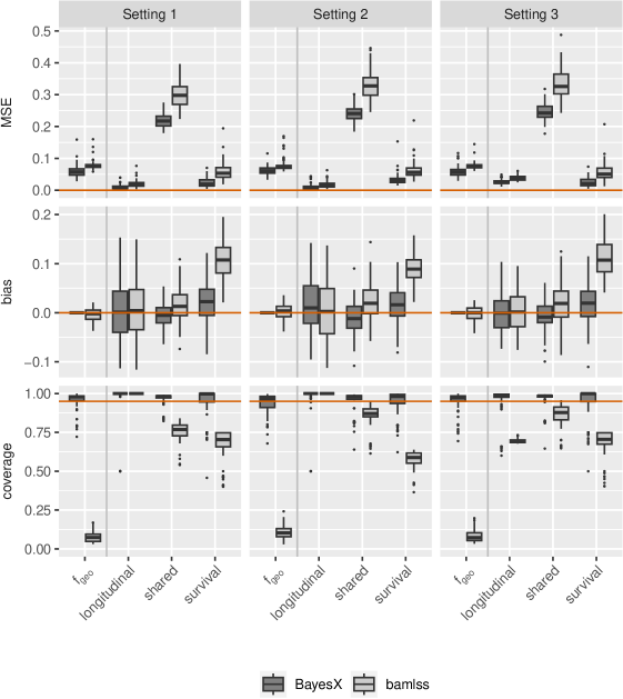
Figure 1: Boxplots of mean squared error (MSE), bias and 95%-coverage for the geographic effect $f_{geo}$ as well as the predictors per method and simulation setting (Setting 1 - $f_{geo}$ in $\eta_{ls}$, Setting 2 - $f_{geo}$ in $\eta_{s}$, Setting 3 - $f_{geo}$ in $\eta_{l}$). The orange horizontal line marks the reference value of each statistic.

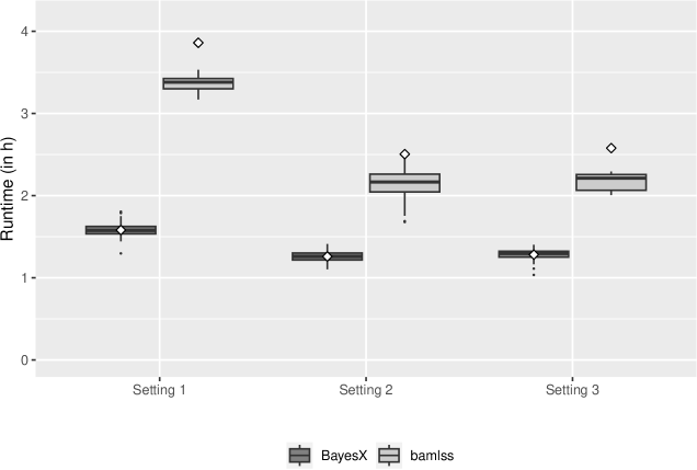
Figure 2: Boxplots of runtimes in hours per method and simulation setting. For readability reasons plots are clipped, therefore extreme outliers are excluded. Diamonds represent respective means. BayesX has visibly lower runtimes than bamlss. With both methods Setting 1 ($f_{geo}$ in $\eta_{ls}$) is the most time consuming, while Setting 2 ($f_{geo}$ in $\eta_{s}$) and 3 ($f_{geo}$ in $\eta_{l}$) are faster and take equally long.

4 Physical Functioning after a Caesura

In 2015 the World Health Organsiation (WHO) concluded in their “World Report on Ageing and Health” that the physical capacity dimension of “Healthy Ageing” still suffers from a lack of understanding. Physical capacity can be measured as functional health (aka physical functioning), which decreases naturally over time until death. However, certain physiological events have the power to alter the trajectory of an individual’s functional health both in a negative and positive way, among them heart attacks, strokes or diagnoses of cancer (caesura, WHO 2015). While the longitudinal modelling of these trajectories is already of interest, the trajectories themselves influence an individual’s survival time. Therefore, a joint model is appropriate to capture both these aspects of the data.
To examine the development of physical functioning after a caesura in Germany we will resort to the German Ageing Survey (DEAS), which aims at studying the second half of life with people between 40 and 85 years old and living in Germany being eligible for study participation. The DEAS has collected information on physical functioning from a SF-36 survey, health conditions qualifying as caesurae, terminal dates and a multitude of other variables, which might help explain the development of physical functioning after a caesura, over the course of seven waves (1996, 2002, 2008, 2011, 2014, 2017, 2021) (Klaus and Engstler 2017; Engstler, Hameister, and Schrader 2014).
Our analysis will focus on data from waves 2008 to 2021 with originally 6622 participants, of which 750 suffered from a heart attack or stroke i.e. a cardiovascular caesura, during their panel participation. Single observations, cases with missing data and caesurae with onset prior to the participant’s entry into the panel were excluded from the analysis. For the remaining 636 the time of onset of the caesura was set to coincide with the interview date, in which the caesura was first reported, since the exact onset date of the caesurae is not collected. Out of 636 participants 79 (12.4%) died.
As explanatory variables for the trajectory of functional health (sf36) we consider time ($\boldsymbol{t}$), gender (gender), the age of onset (aoo) of the caesura as well as living location of the participant on the level of European Nomenclature of Territorial Units for Statistics (NUTS) 2. In order to avoid re-identification of participants few regions had to be combined leaving now 33 regions of the original 36. The continuous and strictly positive variables SF-36 sf36, age of onset aoo and time $\boldsymbol{t}$ are scaled to the domain $(0,1)$. We then consider the model

$$\texttt{sf36}_{i}(t) =\beta_{0}+\boldsymbol{\eta}_{\text{ls}i}+\varepsilon_{i}(t)$$

$$\lambda(t) =\exp\{f_{0}(t)+\alpha\boldsymbol{\eta}_{\text{ls}i}\}$$

$$\boldsymbol{\eta}_{\text{ls}i} =\beta_{1}\texttt{gender}_{i}+f(\texttt{aoo}_{i})+f_{geo}(\texttt{NUTS2}_{i})+\beta_{t}\boldsymbol{t}+b_{0i}+b_{1i}\boldsymbol{t}$$

and estimate it with BayesX and bamlss.

Table 2: BayesX estimates of linear effects of physical functioning after a caesura.

	posterior mean	95%-HDI
$\beta_{0}$	0.848	[0.827, 0.871]
gender	-0.091	[-0.123, -0.059]
$t$	-0.247	[-0.277, -0.219]
$\alpha$	-3.381	[-4.329, -2.432]

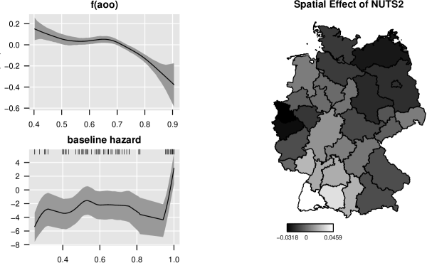
Figure 3: BayesX estimates of the smooth effect of the age of onset aoo and the geographical location on physical functioning as well as the estimated baseline hazard of the model.

With 79 events out of 636 individuals the survival data is unbalanced and presents a situation that - in a standard survival analysis setting - would already prove difficult to estimate. bamlss proved to react sensitive to this imbalance, which is why we only present BayesX results here. For the linear effects they can be found in Table 2 and for the non-linear effects in Figure 3.
None of the linear effects includes zero in their HDI, thus they are significantly different from zero. The association $\alpha$ of both model parts is negative meaning that a lower level of the modelled trajectory of physical functioning sf36 translates to a higher probability of experiencing an event.
The intercept can be interpreted as a male individual at scaled age of 0.402 (i.e. an unscaled age of 40.2) years old at onset of the caesura can be expected to have an average scaled SF-36 level sf36 of 0.848 [0.827, 0.871]. For women this reduces on average by -0.091 [-0.123, -0.059]. Every scaled month after the caesura further reduces the level of sf36 by -0.247 [-0.277, -0.219]. The age of onset aoo has in general a decreasing effect on sf36 (upper left panel Figure 3). Though it needs to be pointed out that before the scaled age of 0.55 (55 years old) the effect is positive, i.e. it increases the level of sf36 thus slowing down the natural decline of physical functioning, while for an aoo between roughly 0.55 and 0.7 (55 to 70 years old) the effect is constant around zero, i.e. it is negligible, and a caesura after an aoo of 0.7 (70 years old) has a negative effect on sf36 translating to an accelerated decline of physical functioning. In terms of living location there is a South-West against North-East (and Mid-West) divide (right panel Figure 3). People in the North-Eastern part of Germany especially in the area of Mecklenburg-Pommerania, Brandenburg and Saxony-Anhalt as well as those of the Western parts in the Dusseldorf and Cologne regions see a negative effect on their level of sf36. Those living in the South-Western part especially in South-West Baden-Wurttemberg (Black Forest region) see an increasing effect on their sf36 level. Given that the association is negative this means that the probability for an event is decreased most for people from the South West of Germany and increased most for those in the North-East and Mid-West. What these two areas have in common is that they comprise the most and least densely populated areas in Germany. This might be a starting point for further research to investigate what exactly triggers the effect to take this particular shape, since the living location in this example can be interpreted as a proxy for other variables that have not been included in the model.
The baseline hazard is almost linear over time (lower left panel Figure 3), thus the risk of experiencing an event is roughly the same at all times throughout the study.

5 Conclusion and Discussion

The focus of this article has been on proposing a piecewise additive joint model for longitudinal and time-to-event data allowing for spatial, (non-)-linear and random effects to be included as well as estimation of the baseline hazard without any assumptions about its distributional form. In a simulation study comprising (non-)linear as well as a spatial effect it became evident that the piecewise additive approach yields results similar or better to the equally flexibly bamlss-methodology for joint models in R and that this performance is high independent of the position of the spatial effect. This method was illustrated by an example of the development of physical functioning after a caesura in people in their second half of life.
The concept of piecewise additive joint models has not just proven its accuracy in estimating complex effects, but also its ability in handling unbalanced data in terms of availability of event observations.
Applying the piecewise additive approach requires augmenting data, which is part of the time-to-event process. This augmentation artificially increases the size of the data set and when the original data is large, it can lead to longer runtimes. In our experience this is, however, seldom the case. Furthermore, this method could also be combined with other models in the longitudinal part of the model such as quantile regression, a location-scale model or multiple longitudinal outcomes in a multivariate joint model. Also, Bayesian variable or effect selection in this type of joint model could be investigated since very few methods for variable selection in joint models exist yet.

Acknowledgement: Elisabeth Bergherr gratefully acknowledges funding from the Deutsche Forschungsgemeinschaft (DFG, German Research Foundation), grant WA 4249/2-1.

References

reAlsefri, Maha, Maria Sudell, Marta García-Fiñana, and Ruwanthi Kolamunnage-Dona. 2020. “Bayesian Joint Modelling of Longitudinal and Time to Event Data: A Methodological Review.” BMC Medical Research Methodology 20 (1): 1–17.

preAndrinopoulou, Eleni-Rosalina, Dimitris Rizopoulos, Johanna J. M. Takkenberg, and Emmanuel Lesaffre. 2014. “Joint Modeling of Two Longitudinal Outcomes and Competing Risk Data.” Statistics in Medicine 33 (18): 3167–78. https://doi.org/https://doi.org/10.1002/sim.6158.

preBarrett, Jessica K, Raphael Huille, Richard Parker, Yuichiro Yano, and Michael Griswold. 2019. “Estimating the Association Between Blood Pressure Variability and Cardiovascular Disease: An Application Using the ARIC Study.” Statistics in Medicine 38 (10): 1855–68.

preBelitz, Christiane, Andreas Brezger, Thomas Kneib, Stefan Lang, and Nikolaus Umlauf. 2022. BayesX: Software for Bayesian Inference in Structured Additive Regression Models. https://www.uni-goettingen.de/de/bayesx/550513.html.

preBender, Andreas, Andreas Groll, and Fabian Scheipl. 2018. “A generalized additive model approach to time-to-event analysis.” Statistical Modelling. https://journals.sagepub.com/doi/10.1177/1471082X17748083.

preBender, Andreas, and Fabian Scheipl. 2018. “pammtools: Piece-wise exponential Additive Mixed Modeling tools.” arXiv:1806.01042 [Stat]. https://arxiv.org/abs/1806.01042.

preBlanche, Paul, Cécile Proust-Lima, Lucie Loubère, Claudine Berr, Jean-François Dartigues, and Hélène Jacqmin-Gadda. 2015. “Quantifying and Comparing Dynamic Predictive Accuracy of Joint Models for Longitudinal Marker and Time-to-Event in Presence of Censoring and Competing Risks.” Biometrics 71 (1): 102–13. https://doi.org/https://doi.org/10.1111/biom.12232.

preCrowther, Michael J., Keith R. Abrams, and Paul C. Lambert. 2013. “Joint Modeling of Longitudinal and Survival Data.” The Stata Journal 13 (1): 165–84. https://doi.org/10.1177/1536867X1301300112.

preEngstler, Heribert, Nicole Hameister, and Sophie Schrader. 2014. “User Manual DEAS SUF 2014.” DZA German Centre of Gerontology.

preFaucett, Cheryl L., Nathaniel Schenker, and Robert M. Elashoff. 1998. “Analysis of Censored Survival Data with Intermittently Observed Time-Dependent Binary Covariates.” Journal of the American Statistical Association 93 (442): 427–37. https://doi.org/10.1080/01621459.1998.10473692.

preFaucett, Cheryl L., and Duncan C. Thomas. 1996. “Simultaneously Modelling Censored Survival Data and Repeatedly Measured Covariates: A Gibbs Sampling Approach.” Statistics in Medicine 15 (15): 1663–85. https://doi.org/10.1002/(SICI)1097-0258(19960815)15:15%3C1663::AID-SIM294%3E3.0.CO;2-1.

preFriedman, Michael. 1982. “Piecewise Exponential Models for Survival Data with Covariates.” The Annals of Statistics 10 (1): 101–13. https://doi.org/10.1214/aos/1176345693.

preGriesbach, Colin, Andreas Groll, and Elisabeth Bergherr. 2021. “Joint Modelling Approaches to Survival Analysis via Likelihood-Based Boosting Techniques.” Computational and Mathematical Methods in Medicine 2021 (November): 4384035.

preHenderson, Robin, Peter Diggle, and Angela Dobson. 2000. “Joint Modelling of Longitudinal Measurements and Event Time Data.” Biostatistics (Oxford, England) 1 (4): 465–80.

preHickey, Graeme L., Pete Philipson, Andrea Jorgensen, and Ruwanthi Kolamunnage-Dona. 2018. “JoineRML: A Joint Model and Software Package for Time-to-Event and Multivariate Longitudinal Outcomes.” BMC Medical Research Methodology 18 (1): 50. https://doi.org/10.1186/s12874-018-0502-1.

preHuang, Xin, Gang Li, Robert M Elashoff, and Jianxin Pan. 2011. “A General Joint Model for Longitudinal Measurements and Competing Risks Survival Data with Heterogeneous Random Effects.” Lifetime Data Analysis 17 (1): 80–100.

preHuang, Yangxin, and Jiaqing Chen. 2016. “Bayesian Quantile Regression-Based Nonlinear Mixed-Effects Joint Models for Time-to-Event and Longitudinal Data with Multiple Features.” Statistics in Medicine 35 (30): 5666–85. https://doi.org/https://doi.org/10.1002/sim.7092.

preJacqmin-Gadda, Hélène, Cécile Proust-Lima, Jeremy M. G. Taylor, and Daniel Commenges. 2010. “Score Test for Conditional Independence Between Longitudinal Outcome and Time to Event Given the Classes in the Joint Latent Class Model.” Biometrics 66 (1): 11–19. https://doi.org/https://doi.org/10.1111/j.1541-0420.2009.01234.x.

preKlaus, Daniela, and Heribert Engstler. 2017. “Daten Und Methoden Des Deutschen Alterssurveys.” In Altern Im Wandel, edited by Katharina Mahne, Julia Katharina Wolff, Julia Simonson, and Clemens Tesch-Römer, 29–45. Wiesbaden; s.l.: Springer Fachmedien Wiesbaden. https://doi.org/10.1007/978-3-658-12502-8/_2.

preKöhler, Meike, Andreas Beyerlein, Kendra Vehik, Sonja Greven, Nikolaus Umlauf, Åke Lernmark, William A Hagopian, et al. 2017. “Joint Modeling of Longitudinal Autoantibody Patterns and Progression to Type 1 Diabetes: Results from the TEDDY Study.” Acta Diabetologica 54 (11): 1009–17.

preKöhler, Meike, Nikolaus Umlauf, Andreas Beyerlein, Christiane Winkler, Anette-Gabriele Ziegler, and Sonja Greven. 2017. “Flexible Bayesian additive joint models with an application to type 1 diabetes research.” Biometrical Journal 59 (6): 1144–65. https://doi.org/https://doi.org/10.1002/bimj.201600224.

preKöhler, Meike, Nikolaus Umlauf, and Sonja Greven. 2018. “Nonlinear association structures in flexible Bayesian additive joint models.” Statistics in Medicine 37 (30): 4771–88. https://doi.org/https://doi.org/10.1002/sim.7967.

preLin, Haiqun, Charles E McCulloch, and Susan T Mayne. 2002. “Maximum Likelihood Estimation in the Joint Analysis of Time-to-Event and Multiple Longitudinal Variables.” Statistics in Medicine 21 (16): 2369–82.

preMartins, Rui, Giovani L. Silva, and Valeska Andreozzi. 2016. “Bayesian joint modeling of longitudinal and spatial survival AIDS data.” Statistics in Medicine 35 (19): 3368–84. https://doi.org/https://doi.org/10.1002/sim.6937.

pre———. 2017. “Joint analysis of longitudinal and survival AIDS data with a spatial fraction of long-term survivors: A Bayesian approach.” Biometrical Journal 59 (6): 1166–83. https://doi.org/https://doi.org/10.1002/bimj.201600159.

preMauff, Katya, Ewout Steyerberg, Isabella Kardys, Eric Boersma, and Dimitris Rizopoulos. 2020. “Joint Models with Multiple Longitudinal Outcomes and a Time-to-Event Outcome: A Corrected Two-Stage Approach.” Statistics and Computing 30: 999–1014.

preR Core Team. 2022. R: A Language and Environment for Statistical Computing. Vienna, Austria: R Foundation for Statistical Computing. https://www.R-project.org/.

preRappl, Anja, Andreas Mayr, and Elisabeth Waldmann. 2022. “More Than One Way: Exploring the Capabilities of Different Estimation Approaches to Joint Models for Longitudinal and Time-to-Event Outcomes.” The International Journal of Biostatistics 18 (1): 127–49. https://doi.org/doi:10.1515/ijb-2020-0067.

preRizopoulos, Dimitris. 2010. “JM: An r Package for the Joint Modelling of Longitudinal and Time-to-Event Data.” Journal of Statistical Software 35 (9). https://doi.org/10.18637/jss.v035.i09.

pre———. 2011. “Dynamic Predictions and Prospective Accuracy in Joint Models for Longitudinal and Time-to-Event Data.” Biometrics 67 (3): 819–29. https://doi.org/10.1111/j.1541-0420.2010.01546.x.

pre———. 2016. “The R Package JMbayes for Fitting Joint Models for Longitudinal and Time-to-Event Data Using MCMC.” Journal of Statistical Software 72 (7). https://doi.org/10.18637/jss.v072.i07.

preRizopoulos, Dimitris, and Pulak Ghosh. 2011. “A Bayesian Semiparametric Multivariate Joint Model for Multiple Longitudinal Outcomes and a Time-to-Event.” Statistics in Medicine 30 (12): 1366–80. https://doi.org/https://doi.org/10.1002/sim.4205.

preRizopoulos, Dimitris, Geert Verbeke, Emmanuel Lesaffre, and Yves Vanrenterghem. 2008. “A Two-Part Joint Model for the Analysis of Survival and Longitudinal Binary Data with Excess Zeros.” Biometrics 64 (2): 611–19. https://doi.org/https://doi.org/10.1111/j.1541-0420.2007.00894.x.

preTseng, Yi-Kuan, Fushing Hsieh, and Jane-Ling Wang. 2005. “Joint modelling of accelerated failure time and longitudinal data.” Biometrika 92 (3): 587–603. https://doi.org/10.1093/biomet/92.3.587.

preTsiatis, Anastasios A., and Marie Davidian. 2004. “Joint Modeling of Longitudinal and Time-to-Event Data: An Overview.” Statistica Sinica 14 (3): 809–34.

preUmlauf, Nikolaus, Nadja Klein, Thorsten Simon, and Achim Zeileis. 2021. “bamlss: A Lego Toolbox for Flexible Bayesian Regression (and Beyond).” Journal of Statistical Software 100 (4): 1–53. https://doi.org/10.18637/jss.v100.i04.

preViviani, Sara, Marco Alfó, and Dimitris Rizopoulos. 2014. “Generalized Linear Mixed Joint Model for Longitudinal and Survival Outcomes.” Statistics and Computing 24 (3): 417–27.

preWaldmann, Elisabeth, David Taylor-Robinson, Nadja Klein, Thomas Kneib, Tania Pressler, Matthias Schmid, and Andreas Mayr. 2017. “Boosting Joint Models for Longitudinal and Time-to-Event Data.” Biometrical Journal 59 (6): 1104–21. https://doi.org/https://doi.org/10.1002/bimj.201600158.

preWHO. 2015. World Report on Ageing and Health. Geneva: World Health Organisation; WHO.

preWulfsohn, Michael S., and Anastasios A. Tsiatis. 1997. “A Joint Model for Survival and Longitudinal Data Measured with Error.” Biometrics 53 (1): 330. https://doi.org/10.2307/2533118.

preYuen, Hok Pan, and Andrew Mackinnon. 2016. “Performance of Joint Modelling of Time-to-Event Data with Time-Dependent Predictors: An Assessment Based on Transition to Psychosis Data.” PeerJ 4: e2582. https://doi.org/10.7717/peerj.2582.

preZhang, Hanze, Yangxin Huang, Wei Wang, Henian Chen, and Barbara Langland-Orban. 2019. “Bayesian Quantile Regression-Based Partially Linear Mixed-Effects Joint Models for Longitudinal Data with Multiple Features.” Statistical Methods in Medical Research 28 (2): 569–88. https://doi.org/10.1177/0962280217730852.

p

Appendix

Appendix A Derivation of the full conditional and IWLS-proposal distributions used for posterior estimation

A.1 Longitudinal effects

Let $\boldsymbol{\gamma}_{\text{l},k}$ be the coefficients of one of $k=1,\dots,p_{\text{l}}$ effects in the longitudinal predictor with a prior as given in (4) and let further denote $\boldsymbol{\eta}_{\text{l, -k}}=\boldsymbol{\eta}_{\text{l}}-\boldsymbol{\eta}_{\text{l, k}}$, i.e. the longitudinal predictor without the $k^{th}$ element. Then the derivation of the full conditionals for this effect follows as:

$$p(\boldsymbol{\gamma}_{\text{l},k}\mid\cdot) \propto p(\boldsymbol{\gamma}_{\text{l}}\mid\sigma^{2}_{\varepsilon},\sigma^{2}_{\boldsymbol{\gamma}_{\text{l}}})\;p(\boldsymbol{y}\mid\boldsymbol{\eta}_{\text{l}},\boldsymbol{\eta}_{\text{ls}},\cdot)$$

$$\propto\exp\left\{-\frac{1}{2\sigma^{2}_{\boldsymbol{\gamma}_{\text{l}}}}\boldsymbol{\gamma}_{\text{l},k}^{\prime}\boldsymbol{K}_{\text{l},k}\boldsymbol{\gamma}_{\text{l},k}\right\}$$

$$\color[rgb]{1,1,1}\propto\color[rgb]{0,0,0}\exp\left\{-\frac{1}{2\sigma^{2}_{\varepsilon}}(\boldsymbol{Z}_{\text{l},k}\boldsymbol{\gamma}_{\text{l},k}-(\boldsymbol{y}-\boldsymbol{\eta}_{\text{l},-k}-\boldsymbol{\eta}_{\text{ls}}))^{\prime}(\boldsymbol{Z}_{\text{l},k}\boldsymbol{\gamma}_{\text{l},k}-(\boldsymbol{y}-\boldsymbol{\eta}_{\text{l},-k}-\boldsymbol{\eta}_{\text{ls}}))\right\}$$

$$\boldsymbol{\gamma}_{\text{l},k}\mid\cdot \sim\text{N}(\mu^{*}_{\boldsymbol{\gamma}_{\text{l},k}},\Sigma^{*}_{\boldsymbol{\gamma}_{\text{l},k}})$$

$$\Sigma^{*}_{\boldsymbol{\gamma}_{\text{l},k}} =\left(\frac{1}{\sigma^{2}_{\varepsilon}}\boldsymbol{Z}_{l,k}^{\prime}\boldsymbol{Z}_{l,k}+\frac{1}{\sigma^{2}_{\boldsymbol{\gamma}_{\text{l},k}}}\boldsymbol{K}_{\text{l},k}\right)^{-1}$$

$$\mu^{*}_{\boldsymbol{\gamma}_{\text{l},k}} =\Sigma^{*}_{\boldsymbol{\gamma}_{\text{l},k}}\left(\frac{1}{\sigma^{2}_{\varepsilon}}\left(\boldsymbol{Z}_{l,k}^{\prime}(\boldsymbol{y}-\boldsymbol{\eta}_{\text{l, -k}}-\boldsymbol{\eta}_{\text{ls}})\right)+\frac{1}{\sigma^{2}_{\boldsymbol{\gamma}_{\text{l},k}}}\boldsymbol{K}_{\text{l},k}\right)$$

A.2 Survival effects

Since the full conditional distribution of the $k^{th}$ survival specific coefficients $p(\boldsymbol{\gamma}_{\text{s},k}\mid\boldsymbol{\delta},\sigma^{2}_{\boldsymbol{\gamma}_{\text{s},k}},\cdot)$ out of $k=1,\dots,p_{\text{s}}$ survival specific effects are analytically intractable, we use MH-steps with IWLS proposals, which approximate the true log-full conditionals. Consider the (standard) full conditional

$$p(\boldsymbol{\gamma}_{\text{s},k}\mid\boldsymbol{\delta},\sigma^{2}_{\boldsymbol{\gamma}_{\text{s},k}},\cdot) \propto p(\boldsymbol{\gamma}_{\text{s},k}\mid\sigma^{2}_{\boldsymbol{\gamma}_{\text{s},k}})\;p(\boldsymbol{\delta}\mid\boldsymbol{\eta}_{\text{s}},\boldsymbol{\eta}_{\text{ls}},\cdot).$$

Let $\boldsymbol{Z}_{\text{s},k}$ be the corresponding design matrix of effect $\boldsymbol{\gamma}_{\text{s},k}$ and $\frac{1}{\sigma^{2}_{\boldsymbol{\gamma}_{\text{s},k}}}\boldsymbol{K}$ the variance statement of prior $p(\boldsymbol{\gamma}_{\text{s},k}\mid\sigma^{2}_{\boldsymbol{\gamma}_{\text{s},k}})$ (compare prior given in (4)). Then draw IWLS proposal $\boldsymbol{\gamma}_{\text{s},k}^{*}$ from a normal distribution density $q(\boldsymbol{\gamma}_{\text{s},k}^{*}\mid\boldsymbol{\gamma}_{\text{s},k}^{[t]})$ with $\boldsymbol{\gamma}_{\text{s},k}^{[t]}$ being the value of $\boldsymbol{\gamma}_{\text{s},k}$ at iteration $t$ of the MCMC algorithm. More specifically

$$\boldsymbol{\gamma}_{\text{s},k}^{*}\sim N\left(\boldsymbol{\mu}^{[t]}_{\boldsymbol{\gamma}_{\text{s},k}},\boldsymbol{P}^{[t]-1}_{\boldsymbol{\gamma}_{\text{s},k}}\right)$$

$$\text{with}\quad\boldsymbol{P}^{[t]}_{\boldsymbol{\gamma}_{\text{s},k}}=\boldsymbol{Z}_{\text{s},k}^{\prime}\boldsymbol{W}^{[t]}_{\text{s}}\boldsymbol{Z}_{\text{s},k}+\frac{1}{\sigma^{2[t]}_{\boldsymbol{\gamma}_{\text{s},k}}}\boldsymbol{K}_{\boldsymbol{\gamma}_{\text{s},k}}\quad\text{and}\quad\boldsymbol{\mu}^{[t]}_{\boldsymbol{\gamma}_{\text{s},k}}=\left(\boldsymbol{P}^{[t]}_{\boldsymbol{\gamma}_{\text{s},k}}\right)^{-1}\boldsymbol{Z}_{\text{s},k}^{\prime}\boldsymbol{W}^{[t]}_{\text{s}}\left(\tilde{\boldsymbol{y}}^{[t]}_{\text{s}}-\boldsymbol{\eta}^{[t]}_{\text{s},-k}\right).$$

Here $\boldsymbol{\eta}^{[t]}_{\text{s},-k}=\boldsymbol{\eta}^{[t]}_{\text{s}}-\boldsymbol{\eta}^{[t]}_{\text{s},k}$, and $\boldsymbol{W}_{\text{s}}^{[t]}$ denotes the working weights and $\tilde{\boldsymbol{y}}_{\text{s}}^{[t]}$ the working observations all evaluated at the current state $t$ of the MCMC chain. The definition of working weights and observations is given further below.
The acceptance probability of the IWLS proposal $\boldsymbol{\gamma}^{*}$ is then

$$\alpha\left(\boldsymbol{\gamma}_{\text{s},k}^{*}\mid\boldsymbol{\gamma}_{\text{s},k}^{[t]}\right)=\min\left\{\frac{L\left(\boldsymbol{\gamma}_{\text{s},k}^{*}\right)\,p\left(\boldsymbol{\gamma}_{\text{s},k}^{*}\right)\,q\left(\boldsymbol{\gamma}_{\text{s},k}^{[t]}\mid\boldsymbol{\gamma}_{\text{s},k}^{*}\right)}{L\left(\boldsymbol{\gamma}_{\text{s},k}^{[t]}\right)\,p\left(\boldsymbol{\gamma}_{\text{s},k}^{[t]}\right)\,q\left(\boldsymbol{\gamma}_{\text{s},k}^{*}\mid\boldsymbol{\gamma}_{\text{s},k}^{[t]}\right)},1\right\}$$

with $L(\boldsymbol{\gamma}_{\text{s},k})=p(\boldsymbol{\delta}\mid\boldsymbol{\gamma}_{\text{s},k},\cdot)$ being the likelihood evaluated at the proposal $\boldsymbol{\gamma}^{*}_{\text{s},k}$ as well as the current state $\boldsymbol{\gamma}^{[t]}$ of the effect.
If the proposal then is accepted it becomes the new state $\boldsymbol{\gamma}_{\text{s},k}^{[t+1]}=\boldsymbol{\gamma}_{\text{s},k}^{*}$, otherwise the current state remains $\boldsymbol{\gamma}_{\text{s},k}^{[t+1]}=\boldsymbol{\gamma}_{\text{s},k}^{[t]}$. Acceptance is established via random draws from a uniform distribution following the logic:

1. Draw $u\sim\text{Unif}(0,1)$
   

2. If $u\leq\alpha$
   then $\boldsymbol{\gamma}^{[t+1]}=\boldsymbol{\gamma}^{*}$
   else $\boldsymbol{\gamma}^{[t+1]}=\boldsymbol{\gamma}^{[t]}$.

For the definition of the working weights and observations consider the log-full conditional

$$\log(p(\boldsymbol{\gamma}_{\text{s},k}\mid\boldsymbol{\delta},\sigma^{2}_{\boldsymbol{\gamma}_{\text{s},k}},\cdot))\propto-\frac{1}{2\sigma^{2}_{\boldsymbol{\gamma}_{\text{s},k}}}\boldsymbol{\gamma}^{\prime}_{\text{s},k}\boldsymbol{K}_{\boldsymbol{\gamma}_{\text{s},k}}\boldsymbol{\gamma}_{\text{s},k}+\ell(\boldsymbol{\eta}_{\text{s}}),$$

where $\ell(\boldsymbol{\eta}_{\text{s}})$ denotes the log-likelihood depending on predictor $\boldsymbol{\eta}_{\text{s}}=\sum_{k=1}^{p_{\text{s}}}\boldsymbol{Z}_{\text{s},k}\boldsymbol{\gamma}_{\text{s},k}$ (compare (3)) thus including $\boldsymbol{\gamma}_{\text{s},k}$. Further, define the score vector $\boldsymbol{v}_{\text{s}}$ as

$$\boldsymbol{v}^{[t]}_{\text{s}}=\frac{\partial\ell(\boldsymbol{\eta}^{[t]}_{\text{s}})}{\partial\boldsymbol{\eta}^{[t]}_{\text{s}}},$$

i.e. the vector of first derivatives of $\ell(\boldsymbol{\eta}_{\text{s}})$ with respect to the predictor $\boldsymbol{\eta}_{\text{s}}$ evaluated at the current iteration $t$ and the working weights also evaluated at iteration $t$ as

$$\boldsymbol{W}^{[t]}_{\text{s}}=\text{diag}\left(w_{1}\left(\eta_{\text{s},1}^{[t]}\right),\dots,w_{n_{a}}\left(\eta_{\text{s},n_{a}}^{[t]}\right)\right)$$

with $n_{a}$ the number of observations in the augmented dataset (compare Section 2.2 Table 1) and

$$w_{i}\left(\eta_{\text{s},i}^{[t]}\right)=-\text{E}\left(\frac{\partial\ell(\eta^{[t]}_{\text{s},i})}{\partial^{2}\eta^{[t]}_{\text{s},i}}\right)=-\text{E}\left(\frac{\partial v^{[t]}_{\text{s},i}}{\partial\eta^{[t]}_{\text{s},i}}\right).$$

The vector of working observations $\tilde{\boldsymbol{y}}^{[t]}_{\text{s}}=\left(\tilde{y}_{\text{s}1}\left((\eta_{1}^{[t]}\right),\dots,\tilde{y}_{\text{s}n_{a}}\left(\eta_{n_{a}}^{[t]}\right)\right)^{\prime}$ is then determined by

$$\tilde{\boldsymbol{y}}^{[t]}_{\text{s}}=\boldsymbol{\eta}^{[t]}_{\text{s}}+\left(\boldsymbol{W}_{\text{s}}^{[t]}\right)^{-1}\boldsymbol{v}^{[t]}_{\text{s}}.$$

A.3 Shared effects

The full conditional of the $k^{th}$ coefficient $p(\boldsymbol{\gamma}_{\text{ls},k}\mid\boldsymbol{y},\boldsymbol{\delta},\sigma^{2}_{\boldsymbol{\gamma}_{\text{ls},k}},\cdot)$ of the $k=1,\dots,p_{\text{ls}}$ shared effects are neither tractable. Therefore, we also apply an MH-step with IWLS-proposal here. The procedure is similar to the survival specific coefficients but needs to consider the joint likelihood of both model parts. First consider the full conditional

$$p\left(\boldsymbol{\gamma}_{\text{ls, k}}\mid\cdot\right)\propto p(\boldsymbol{\gamma}_{\text{ls, k}}\mid\sigma^{2}_{\boldsymbol{\gamma}_{\text{ls}}})\;p(\boldsymbol{y}\mid\boldsymbol{\eta}_{\text{l}},\boldsymbol{\eta}_{\text{ls}},\cdot)\;p(\boldsymbol{\delta}\mid\boldsymbol{\eta}_{\text{s}},\boldsymbol{\eta}_{\text{ls}},\cdot).$$

Let $\boldsymbol{Z}_{\text{ls},k}$ be the corresponding design matrix of effect $\boldsymbol{\gamma}_{\text{ls},k}$ and $\frac{1}{\sigma^{2}_{\boldsymbol{\gamma}_{\text{ls},k}}}\boldsymbol{K}$ the variance statement of prior $p(\boldsymbol{\gamma}_{\text{ls},k}\mid\sigma^{2}_{\boldsymbol{\gamma}_{\text{ls},k}})$ (compare prior given in (4)). Now to approximate the full conditional we draw IWLS proposal $\boldsymbol{\gamma}_{\text{ls},k}^{*}$ from a normal distribution density $q(\boldsymbol{\gamma}_{\text{ls},k}^{*}\mid\boldsymbol{\gamma}_{\text{ls},k}^{[t]})$ with $\boldsymbol{\gamma}_{\text{ls},k}^{[t]}$ being the value of $\boldsymbol{\gamma}_{\text{ls},k}$ at iteration $t$ of the MCMC algorithm. More specifically

$$\boldsymbol{\gamma}_{\text{ls},k}^{*}\sim N\left(\boldsymbol{\mu}^{[t]}_{\boldsymbol{\gamma}_{\text{ls},k}},\left(\boldsymbol{P}^{[t]}_{\boldsymbol{\gamma}_{\text{ls},k}}\right)^{-1}\right)$$

$$\text{with}\quad\boldsymbol{P}^{[t]}_{\boldsymbol{\gamma}_{\text{ls},k}}=\boldsymbol{Z}_{\text{ls},k}^{\prime}\boldsymbol{W}_{\text{ls}}^{[t]}\boldsymbol{Z}_{\text{ls},k}+\frac{1}{\sigma^{2[t]}_{\boldsymbol{\gamma}_{\text{ls},k}}}\boldsymbol{K}_{\boldsymbol{\gamma}_{\text{ls},k}}\quad\text{and}\quad\boldsymbol{\mu}^{[t]}_{\boldsymbol{\gamma}_{\text{ls},k}}=\left(\boldsymbol{P}^{[t]}_{\boldsymbol{\gamma}_{\text{ls},k}}\right)^{-1}\boldsymbol{Z}_{\text{ls},k}^{\prime}\boldsymbol{W}_{\text{ls}}^{[t]}\left(\tilde{y}_{\text{ls}}^{[t]}-\boldsymbol{\eta}_{\text{ls},-k}^{[t]}\right).$$

The rest of the algorithm is analogous to the survival effects.

To see how the working weights and observations build for the coefficients in the shared predictor, consider first the log-full conditional

$$\log(p(\boldsymbol{\gamma}_{\text{ls},k}\mid\boldsymbol{y},\boldsymbol{\delta},\sigma^{2}_{\boldsymbol{\gamma}_{\text{ls},k}},\cdot))\propto-\frac{1}{2\sigma^{2}_{\boldsymbol{\gamma}_{\text{ls},k}}}\boldsymbol{\gamma}^{\prime}_{\text{ls},k}\boldsymbol{K}_{\boldsymbol{\gamma}_{\text{ls},k}}\boldsymbol{\gamma}_{\text{ls},k}+\ell_{y}(\boldsymbol{\eta}_{\text{ls}})+\ell_{\delta}(\boldsymbol{\eta}_{\text{ls}}),$$

where $\ell_{y}(\boldsymbol{\eta}_{\text{ls}})$ denotes the longitudinal part of the log-likelihood and $\ell_{\delta}(\boldsymbol{\eta}_{\text{ls}})$ the survival/ poisson part of the log-likelihood depending on predictor $\boldsymbol{\eta}_{\text{ls}}=\sum_{k=1}^{p_{\text{ls}}}\boldsymbol{Z}_{\text{ls},k}\boldsymbol{\gamma}_{\text{ls},k}$ (compare (3)) thus including $\boldsymbol{\gamma}_{\text{ls},k}$.

The vector of scores, i.e. first derivatives of the log-likelihoods with respect to $\boldsymbol{\eta}_{\text{ls}}$ evaluated at iteration $t$, is

$$\boldsymbol{v}^{[t]}_{\text{ls}}=\boldsymbol{v}^{[t]}_{y,\text{ls}}+\alpha\boldsymbol{v}^{[t]}_{\delta,\text{ls}}=\frac{\partial\ell_{y}(\boldsymbol{\eta}^{[t]}_{\text{ls}})}{\partial\boldsymbol{\eta}^{[t]}_{\text{ls}}}+\frac{\partial\ell_{\delta}(\boldsymbol{\eta}^{[t]}_{\text{ls}})}{\partial\boldsymbol{\eta}^{[t]}_{\text{ls}}}.$$

The working weights evaluated at iteration $t$ can then be derived as

$$\boldsymbol{W}^{[t]}_{\text{ls}}=\text{diag}\left(w_{1}\left(\eta_{\text{ls},1}^{[t]}\right),\dots,w_{n_{a}}\left(\eta_{\text{ls},n_{a}}^{[t]}\right)\right)$$

with $n_{a}$ the number of observations in the augmented dataset and

$$w_{i}(\eta_{\text{ls},i}^{[t]}) =-\text{E}\left(\frac{\partial v^{[t]}_{\text{ls},i}}{\partial\eta^{[t]}_{\text{ls},i}}\right)=-\text{E}\left(\frac{\partial\boldsymbol{v}^{[t]}_{y,\text{ls},i}+\alpha\boldsymbol{v}^{[t]}_{\delta,\text{ls},i}}{\partial\eta^{[t]}_{\text{ls},i}}\right)=-\text{E}\left(\frac{\partial\ell_{y}(\boldsymbol{\eta}^{[t]}_{\text{ls},i})}{\partial^{2}\boldsymbol{\eta}^{[t]}_{\text{ls},i}}\right)-\text{E}\left(\frac{\partial\ell_{\delta}(\boldsymbol{\eta}^{[t]}_{\text{ls},i})}{\partial^{2}\boldsymbol{\eta}^{[t]}_{\text{ls},i}}\right)$$

$$=w_{y,i}(\eta_{\text{ls},i}^{[t]})+\alpha^{2}w_{\delta,i}(\eta_{\text{ls},i}^{[t]}).$$

The working observations then follow analogously as

$$\tilde{\boldsymbol{y}}_{\text{ls}}^{[t]}=\boldsymbol{\eta}^{[t]}_{\text{ls}}+\left(\boldsymbol{W}_{\text{ls}}^{[t]}\right)^{-1}\boldsymbol{v}^{[t]}_{\text{ls}}.$$

A.4 Variances

A.4.1 Model variance

Let $N=\sum_{i=1}^{n}n_{i}$ be the total number of longitudinal observations as the sum of all observations $n_{i}$ per individual $i$ across all individuals $n$. Then the full conditional of the model variance follows as

$$p(\sigma^{2}_{\varepsilon}\mid\cdot) \propto p(\sigma^{2}_{\varepsilon})\;p(\boldsymbol{y}\mid\boldsymbol{\eta}_{\text{l}},\boldsymbol{\eta}_{\text{ls}},\sigma^{2}_{\varepsilon})$$

$$\propto(\sigma^{2}_{\varepsilon})^{-a_{0}-1}\;\exp\left\{-\textstyle{\frac{b_{0}}{\sigma^{2}_{\varepsilon}}}\right\}$$

$$\color[rgb]{1,1,1}\propto\color[rgb]{0,0,0}\left(\sigma^{2}_{\varepsilon}\right)^{-\frac{N}{2}}\;\exp\left\{-\textstyle{\frac{1}{2\sigma^{2}_{\varepsilon}}}(\boldsymbol{y}-\boldsymbol{\eta}_{\text{l}}-\boldsymbol{\eta}_{\text{ls}})^{\prime}(\boldsymbol{y}-\boldsymbol{\eta}_{\text{l}}-\boldsymbol{\eta}_{\text{ls}})\right\}$$

$$\propto\left(\sigma^{2}_{\varepsilon}\right)^{-(a_{0}+\frac{N}{2})-1}\;\exp\left\{-\textstyle{\frac{1}{\sigma^{2}_{\varepsilon}}}(b_{0}+\textstyle{\frac{1}{2}}(\boldsymbol{y}-\boldsymbol{\eta}_{\text{l}}-\boldsymbol{\eta}_{\text{ls}})^{\prime}(\boldsymbol{y}-\boldsymbol{\eta}_{\text{l}}-\boldsymbol{\eta}_{\text{ls}}))\right\}$$

$$\sigma^{2}_{\varepsilon}\mid\cdot \sim\text{IG}\left(a_{0}+\textstyle{\frac{N}{2}},b_{0}+(\boldsymbol{y}-\boldsymbol{\eta}_{\text{l}}-\boldsymbol{\eta}_{\text{ls}})^{\prime}(\boldsymbol{y}-\boldsymbol{\eta}_{\text{l}}-\boldsymbol{\eta}_{\text{ls}})\right)$$

A.4.2 Variance of coefficients

With $p_{\cdot}$ being the number of covariates in each predictor(longitudinal, shared, survival) the full conditional of the $k_{\cdot}=1,\dots,p_{\cdot}$ variances of the corresponding effects is

$$p(\sigma^{2}_{\boldsymbol{\gamma}_{k_{\cdot}}}\mid\cdot) \propto p(\sigma^{2}_{\boldsymbol{\gamma}_{k_{\cdot}}})\;p(\boldsymbol{\gamma}_{k_{\cdot}}\mid\sigma^{2}_{\boldsymbol{\gamma}_{k_{\cdot}}})$$

$$\propto(\sigma^{2}_{\boldsymbol{\gamma}_{k_{\cdot}}})^{-a_{k_{\cdot}}-1}\;\exp\left\{-\textstyle{\frac{b_{k_{\cdot}}}{\sigma^{2}_{\boldsymbol{\gamma}_{k_{\cdot}}}}}\right\}$$

$$\color[rgb]{1,1,1}\propto\color[rgb]{0,0,0}\left(\sigma^{2}_{\boldsymbol{\gamma}_{k_{\cdot}}}\right)^{-\text{rk}\boldsymbol{K}_{k_{\cdot}}}\;\exp\left\{-\textstyle{\frac{1}{2\sigma^{2}_{\boldsymbol{\gamma}_{k_{\cdot}}}}}\boldsymbol{\gamma}_{\cdot,k_{\cdot}}^{\prime}\boldsymbol{K}_{k_{\cdot}}\boldsymbol{\gamma}_{\cdot,k_{\cdot}}\right\}$$

$$\propto\left(\sigma^{2}_{\boldsymbol{\gamma}_{k_{\cdot}}}\right)^{-(a_{k_{\cdot}}+\text{rk}\boldsymbol{K}_{k_{\cdot}})-1}\;\exp\left\{-\textstyle{\frac{1}{\sigma^{2}_{\boldsymbol{\gamma}_{k_{\cdot}}}}}(b_{k_{\cdot}}+\boldsymbol{\gamma}_{\cdot,k_{\cdot}}^{\prime}\boldsymbol{K}_{k_{\cdot}}\boldsymbol{\gamma}_{\cdot,k_{\cdot}})\right\}$$

$$\sigma^{2}_{\boldsymbol{\gamma}_{k_{\cdot}}}\mid\cdot \sim\text{IG}\left(a_{k_{\cdot}}+\text{rk}\boldsymbol{K}_{k_{\cdot}},b_{k_{\cdot}}+\boldsymbol{\gamma}_{\cdot,k_{\cdot}}^{\prime}\boldsymbol{K}_{k_{\cdot}}\boldsymbol{\gamma}_{\cdot,k_{\cdot}}\right)$$

Appendix B Detailed results of simulations study

Figure 4 displays the results of the simulation study detailed by individual effect.

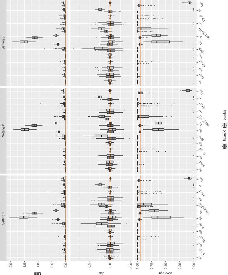
Figure 4: Boxplots of mean squared error (MSE), bias and 95$\%$-coverage per method by effect and simulation setting (Setting 1 - $f_{geo}$ in $\eta_{ls}$, Setting 2 - $f_{geo}$ in $\eta_{s}$, Setting 3 - $f_{geo}$ in $\eta_{l}$). The orange horizontal line marks the reference value of each statistic.

Appendix C Statistical overview of run times

Table 3 details descriptive measures of the run times.

Table 3: Statistical overview of run times of 100 replications per setting and estimation method.

Method	Min.	1st.Qu.	Median	Mean	3rd.Qu.	Max.
Setting 1
BayesX	1.30	1.53	1.58	1.58	1.62	1.80
bamlss	3.17	3.30	3.38	3.86	3.42	10.62
Setting 2
BayesX	1.10	1.22	1.26	1.26	1.30	1.41
bamlss	1.68	2.04	2.17	2.50	2.26	9.62
Setting 3
BayesX	1.03	1.25	1.30	1.28	1.32	1.40
bamlss	2.01	2.06	2.21	2.58	2.26	12.98