Data Release of the AST3-2 Automatic Survey from Dome A, Antarctica

Abstract

AST3-2 is the second of the three Antarctic Survey Telescopes, aimed at wide-field time-domain optical astronomy. It is located at Dome A, Antarctica, which is by many measures the best optical astronomy site on the Earth’s surface. Here we present the data from the AST3-2 automatic survey in 2016 and the photometry results. The median 5$\sigma$ limiting magnitude in $i$-band is 17.8 mag and the light curve precision is 4 mmag for bright stars. The data release includes photometry for over 7 million stars, from which over 3,500 variable stars were detected, with 70 of them newly discovered. We classify these new variables into different types by combining their light curve features with stellar properties from surveys such as StarHorse.

1 Introduction

Time-domain astronomy has led to many astronomical discoveries through exploring the variability of astronomical objects over time. Transient targets such as supernovae (SNe), gamma-ray bursts, and tidal disruption events (TDEs) give valuable insights in astronomy and fundamental physics. Many survey projects have been undertaken to search for variable sources by repeatedly scanning selected sky areas. Deep surveys over wide areas of sky require specialized telescopes such as the Large Binocular Telescope (LBT; Hill & Salinari 2000) and the Large Synoptic Survey Telescope (LSST; Ivezic et al. 2008), and results from such surveys will doubtless make revolutionary discoveries in coming years. High cadence is also important for time-domain surveys when searching for transients such as exoplanets, rapidly-changing objects, and short-term events. The Wide Angle Search for Planets (WASP; Pollacco et al. 2006) consortium has discovered numerous exoplanets with its high cadence. The Zwicky Transient Facility (ZTF; Bellm et al. 2019) has discovered over 3,000 supernovae from its first year of operations with a cadence as rapid as 3 days.

The Antarctic plateau is an ideal site for ground-based time-domain astronomy with its long clear polar nights that can provide long-term continuous observing time as well as other excellent observing conditions (Storey 2005, 2007; Ashley 2013). The clean air can minimize the scattering of light, the cold air is good for infrared observations due to the low thermal background, and the stable atmosphere provides remarkably good seeing.

As the highest location on the Antarctic ice cap, Dome A was first reached by the 21st CHInese National Antarctic Research Expedition (CHINARE) in 2005. It is also the place where the Chinese Kunlun station was established. Many site testing studies have been conducted here during the past decade, and the results have confirmed that Dome A is an excellent site for astronomical observations. A complete summary of the astronomy-related work at Dome A can be found in Shang (2020). We present some important results briefly below.

The Chinese Small Telescope ARray (CSTAR) showed that the median $i$-band sky background of moonless clear nights is 20.5 mag arcsec^-2 (Zou et al., 2010). The KunLun Cloud and Aurora Monitor (KLCAM) showed that the nighttime clear sky rate is 83 per cent, which is better than most ground-based sites (Yang et al., 2021). Moreover, the Surface layer NOn-Doppler Acoustic Radar (SNODAR; Bonner et al. 2010) showed a very shallow atmospheric turbulent boundary layer at Dome A, with a median thickness of only 13.9 m. The multilayer Kunlun Automated Weather Station (KLAWS) showed that a temperature inversion often occurs near the ground, which leads to a stable atmosphere where cooler air is trapped under warmer air (Hu et al., 2014, 2019). The results from SNODAR and KLAWS suggest that extremely good seeing is relatively easy to obtain at Dome A since the telescope only has to be above the shallow turbulent boundary layer to achieve free-atmosphere conditions. This is impractical at traditional observatory sites where the boundary layer is typically many hundreds of metres above the ground. In 2019, the two KunLun Differential Image Motion Monitors (KL-DIMMs) directly confirmed these ideas by measuring the seeing at Dome A from an 8 m tall tower. Superb night-time seeing as good as 0.13″was recorded. The median free-atmosphere seeing was 0.31″and the KL-DIMMs reached the free atmosphere from the 8m tower 31% of the time (Ma et al., 2020b). In summary, the studies described above have demonstrated that by many measures Dome A has the best optical observational conditions from the Earth’s surface.

With such exceptional observing conditions, telescopes were planned and constructed to operate at Dome A for time-domain astronomy. The first-generation optical telescope, CSTAR, was installed in 2008 January (Yuan et al., 2008; Zhou et al., 2010). It observed a 20 deg² sky area centred at the South Celestial Pole with four co-aligned 14.5cm telescopes. CSTAR obtained data for three years and has contributed to many studies on stellar variability (Wang et al., 2011; Yang et al., 2015; Zong et al., 2015; Liang et al., 2016; Oelkers et al., 2016). The three Antarctic Survey Telescopes (AST3; Cui et al. 2008) were later planned as the second-generation optical telescopes at Dome A, with larger apertures and the ability to point and track over the sky, as opposed to CSTAR’s conservative engineering approach of having a fixed altitude.

The first AST3 telescope (AST3-1) was installed at Dome A in 2012 by the 28th CHINARE. AST3-1 surveyed a sky area of roughly 2000 deg² and the data have been released (Ma et al., 2018). AST3-1 also monitored some specific sky regions such as the Large and Small Magellanic Clouds. These data were used for research on exoplanets and variable stars. For example, AST3-1 detected about 500 variable stars around the Galactic disk centre, with 339 of them being newly discovered (Wang et al., 2017a).

The AST3 telescopes were originally conceived as multi-band survey telescopes operating together, but the goal has not been achieved due to various logistic difficulties, such as the required amount of electrical power. The second AST3 telescope (AST3-2) was installed in 2015 by the 31st CHINARE. This work is based on the data from AST3-2. The third AST3 (AST3-3) has been constructed and will be equipped with a K-dark infrared camera (Burton et al., 2016; Li et al., 2016).

Here we present the data and photometry from the AST3-2 sky survey as well as an analysis of the light curves. We first present the basic design of AST3-2 in section 2 and go on to discuss the survey parameters and operational strategy in section 3. In section 4 we discuss the data reduction process and results. In section 5 we present the light curves, the result of period searches, and the classification of objects. The overall statistics of the catalogue and data access are discussed in section 6. Finally, we summarize the results in section 7.

2 Instrument

The details of the AST3 system have been presented in previous works (Yuan et al., 2010; Yuan & Su, 2012; Yuan et al., 2014). Here we briefly describe the basic features of the AST3-2, the second telescope of AST3.

AST3-2 has the same modified Schmidt optical design as the AST3-1. It has a 680mm primary mirror, an entrance pupil diameter of 500mm, a 3.73 f-ratio, and an SDSS $i$ filter. The AST3 telescopes were designed specially to work in the harsh environment of Dome A where the ambient temperature in the observation season ranges from $-80\degr$C to $-50\degr$C. The AST3 telescopes and the mounting system were built with low thermal expansion materials such as Invar to minimize the thermal effects. This design enables the AST3-2 to work in extremely low temperatures, but we still had occasional problems with gears being stuck or jammed by ice. To cope with optical element frosting problems that are common in Antarctica, a defrosting system was designed with an indium-tin-oxide (ITO) coating on the entrance aperture to the telescope and a warm blower inside the tube. However, in the first year of operation, the frosting problem on the first surface was not completely solved. The ITO coating was sometimes insufficient to defrost the ice and the blow heater had to work frequently, resulting in significant tube seeing and poor image quality. To solve this problem, an external defrosting blower system was installed in front of the telescope in 2016.

AST3-2 is equipped with a 10K $\times$ 10K STA1600FT CCD with a pixel size of 9µm. There are 16 read-out channels for the CCD to reduce the read-out time, which is 2.5s in fast read-out mode and 40s in slow read-out mode. To prevent shutter failure in cold weather, the camera works without a mechanical shutter, instead relying on frame-transfer mode and dedicating half of the CCD area to a buffer that is not exposed to light. The astronomically usable area of the CCD is therefore 10K $\times$ 5K pixels, with a scale of  1″/pixel over a FOV of 2.93°$\times$ 1.47°. Since the CCD camera is installed inside the telescope tube, it also faced some heat dissipation problems, causing the CCD to often operate at temperatures as warm as -50$\degr$C to -40$\degr$C, leading to a significant dark current. Since we could not take dark frames on-site and the previously-taken laboratory dark images have different patterns, a new method was developed to derive a dark frame from the science images and will be discussed in section 4.1.2. There was also a problem with the AST3 CCD in that the photon transfer curve became non-linear at a level around 25000 ADU, leading to the brighter-fatter effect (Ma et al., 2014d). Fig. 1 shows a raw image taken by AST3-2. Detailed laboratory tests of the CCD performance can be found in Ma et al. (2012) and Shang et al. (2012).

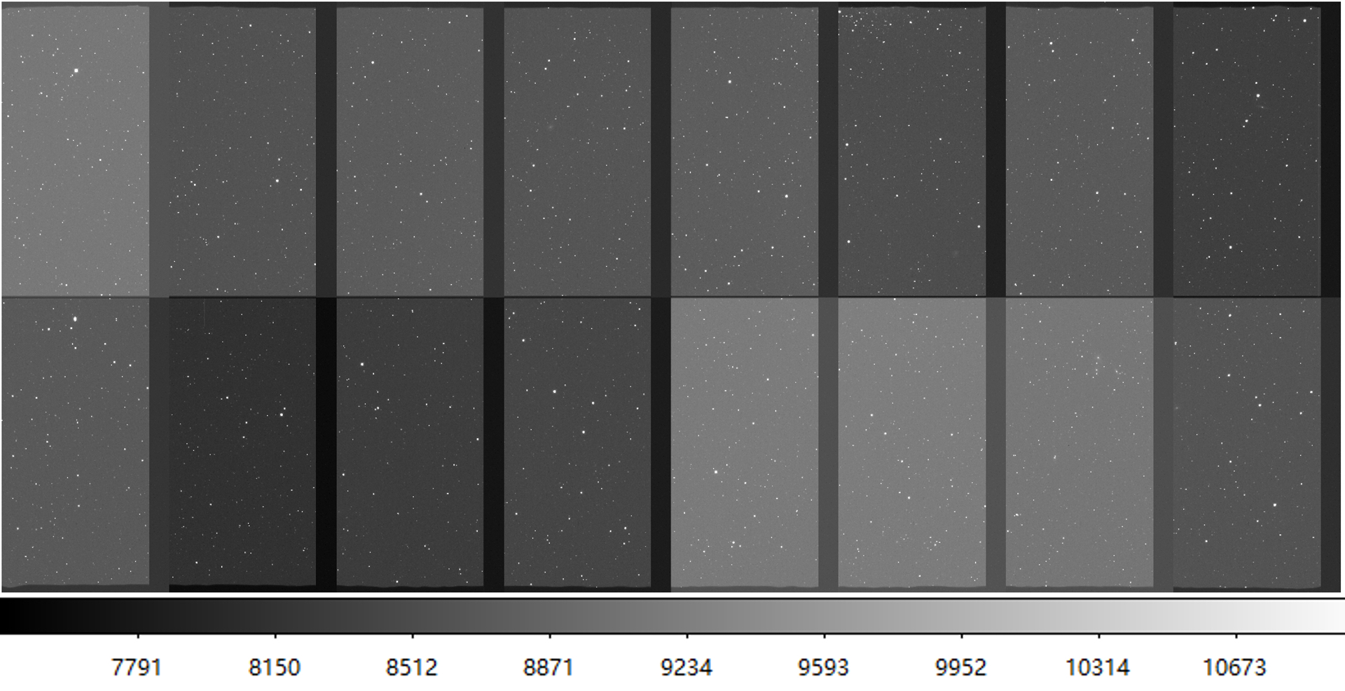
Figure 1: An example of a raw image that is taken from the survey fields by AST3-2. There are 16 readout channels with different bias levels and overscan regions. The lower 8 channels are read out towards the bottom of the CCD, and the upper 8 channels are read out towards the top. Each of the readouts has an area of 1500 pixels $\times$ 2660 pixels including overscan. The overscan regions have 180 columns on the right of each readout and 20 horizontal rows in the middle of the image.

The AST3-2 is powered by the PLATeau Observatory for Dome A (PLATO-A; Ashley et al. 2010). PLATO-A is a self-contained automated platform providing an average power of 1kW for at least 1 year. It also provides Internet access through the Iridium satellite constellation. The hardware and software of the control, operation, and data system (CODS) of AST3-2 were designed to be responsible for the automated sky survey (Shang et al., 2012; Hu et al., 2016a; Shang et al., 2016; Ma et al., 2020a). The CODS consists of the main control system, the data storage array, and the pipeline system. To ensure the success of the sky survey, we developed the CODS to be stable and reliable under the conditions of low power availability (1 kW), low data bandwidth (a maximum of about 2 GB over the course of the year), and the unattended situation in the harsh winter of Dome A. The supporting software provides a fully automatic survey control and a real-time data processing pipeline on-site.

3 Observations and Data

The observing season at Dome A starts in mid-March when the Sun reaches 13 degrees below the horizon, i.e., at the end of twilight (Zou et al., 2010). The automated and unattended AST3 sky survey strategy was designed to optimize the available observing time and was realized with a survey scheduler in the CODS software (Liu et al., 2018). The scheduler provides three different survey modes depending on the scientific requirements. The SN survey mode mainly focuses on a survey for SNe and other transients, the exoplanet search mode aims at discovering and monitoring short-period exoplanets, and an additional special mode mainly targets the follow-up of transients.

Following twilight, the AST3-2 was initially dedicated to the SN survey mode, lasting from 2016 March 24 to May 16, at which point the long continuous polar night began and the survey switched to exoplanet mode. The SN survey was designed for the early discovery of SNe as well as other transients, and for time-domain astronomy of variable stars. It surveyed sky areas of 2200 deg², covering 565 fields with about 30 visits each in a cadence of a half to a few days based on the fraction of dark time within a day. Fig. 2 shows the sky coverage of this survey. The real-time pipeline from CODS performed onsite data reduction and sent the SN or other transient candidates back to China for further confirmation and follow-up observations. For example, the real-time pipeline discovered the SN 2016ccp (Hu et al., 2016b) and the Type IIP SN 2017fbq (Wang et al., 2017b). During the test observations in Mohe, China, the AST3-2 recorded the SN 2014J in M82(Ma et al., 2014b) and discovered the type Ia SN 2014M (Ma et al., 2014a). The real-time pipeline is also capable of detecting other variables such as dwarf novae (Ma et al., 2016), although most of the variables were not reported in the real-time pipeline. So in this work, we mainly use the SN survey mode data when the hard disks were physically returned from Dome A to obtain the photometric catalogue and light curves of other variables.

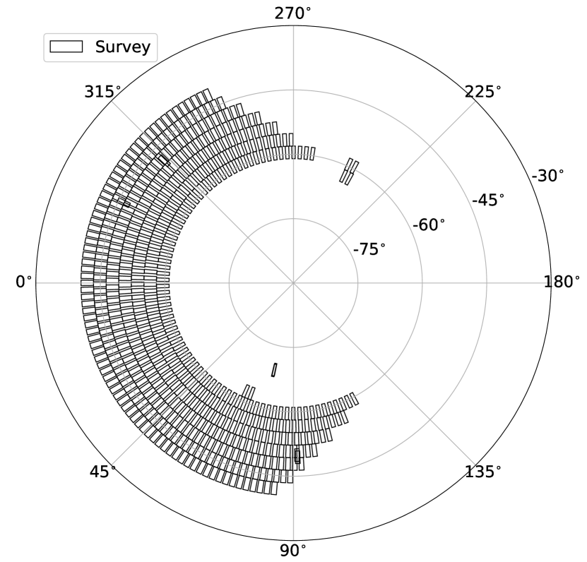
Figure 2: The sky coverage of survey observations from AST3-2 in 2016. Each rectangle region is a target sky field based on the survey scheduler.

The AST3-2 exoplanet project is named the CHinese Exoplanet Searching Program from Antarctica (CHESPA). To search for short-period exoplanets rapidly and continuously, the exoplanet search mode started during the period of continuous dark polar nights: from May 16 to June 22. The exoplanet search covered a smaller sky area than the SN survey, with 10 to 20 fields in each target region. The target region during 2016 contained 10 adjacent fields from the southern continuous viewing zone of TESS (Ricker et al., 2009). This part of the data has been analysed in previous works (Zhang et al., 2019a, b; Liang et al., 2020).

Finally, a special mode was designed for the rapid follow-up of observations of interesting transients from the AST3-2 SN or exoplanet surveys, or from surveys by other telescopes. This mode has the highest priority. When an interesting target triggers the alert, it will pause other observations and resume them after the special observation is finished. In 2017, AST3-2 successfully detected the first optical counterpart of the gravitational wave source GW170817 (Hu et al., 2017).

4 Data Reduction

The 2016 data of AST3-2 was retrieved by the 33rd CHINARE. We focus on the SN survey data for this work. First, we carried out the image corrections for CCD image pre-processing, cross-talk, image trimming, overscan, dark current, flat-field, and an unusual diagonal stripey noise described below. Then we performed photometric and astrometric calibration to obtain the source catalogue. Finally, we cross-matched the catalogues to obtain the light curves. Details of the data reduction process are discussed in the subsections below.

4.1 Preprocessing

4.1.1 Image trimming and overscan subtraction

The AST3 raw image has 12000 $\times$ 5300 pixels including overscan regions and is divided into 16 channels with a size of 1500 $\times$ 2650 each. As described in section 2, the AST3 CCD works in frame-transfer mode, which means it does not have a shutter. Since the zero-second exposure is not a true zero because the frame transfer period takes time, photons would be gathered in the 0s bias frame when there is no shutter. This design makes it hard to take a bias frame on-site. Instead, we used the overscan regions to remove the effect of the bias voltage. As Fig. 1 shows, the overscan regions are the right 180 columns of each channel and 20 rows in the middle of the full raw image.

Because the top and bottom rows of the CCD are insensitive to light, we removed another 80 rows each from the top and bottom of the CCD full images. After overscan correction and image trimming, the final raw images have a size of 10560 $\times$ 5120 pixels.

4.1.2 Dark current subtraction

As described in section 2, the CCD temperature was not very stable and could be above $-50^{\circ}$C sometimes, making the dark current non-negligible. Moreover, the laboratory dark images had different patterns and were not usable for dark correction in practice. Additionally, we could not take dark frames on site because the CCD does not have a shutter and the AST3 was unattended for at least one year. Therefore, a new method was developed to derive the dark frame from scientific images to solve this problem and it had been successfully applied to the AST3-1 images (Ma et al., 2014c, 2018). Here we briefly describe this method and how we utilized it in the AST3-2 preprocessing.

The brightness $I$ of a pixel $(x,y)$ can be described as follow:

$$I(x,y)=S_{T}+D(T)+\Delta d(T,x,y),$$ (1)

where $S_{T}$ is the sky background, $D(T)$ is the median dark current level at temperature $T$, and $\Delta d(T,x,y)$ is the deviation from the median dark current in pixel $(x,y)$ at temperature $T$. The stars can be ignored by a median algorithm if we combine large numbers of images from different sky fields. For a single image, $D(T)$ can be considered constant. Also, the sky brightness can be considered a constant because it is spatially flat enough after twilight (Yang et al., 2017). The first two terms on the right-hand side of the equation (1) can be considered constant for a single image. To derive the distribution of the deviation from the median dark current level $\Delta d(T,x,y)$, we need to take two scientific images that were taken at the same temperature but with different sky brightnesses. By scaling the two images to an equivalent median level and subtracting one from another, we can derive a $\Delta d(T,x,y)$ image at a specific temperature $T$. We repeated this process for different pairs of images at the same $T$ and combined the dark images to construct a master dark image for the specific temperature $T$. Fig.  3 shows the master dark image derived from the 2016 observations.

For different temperatures, the dark current level doubles as the temperature increases every 7.3^∘ for the AST3 CCD between $-80^{\circ}$ and $-40^{\circ}$ (Ma et al., 2012). We used this relation to scale the master dark image to different temperatures and correct the dark current for all images.

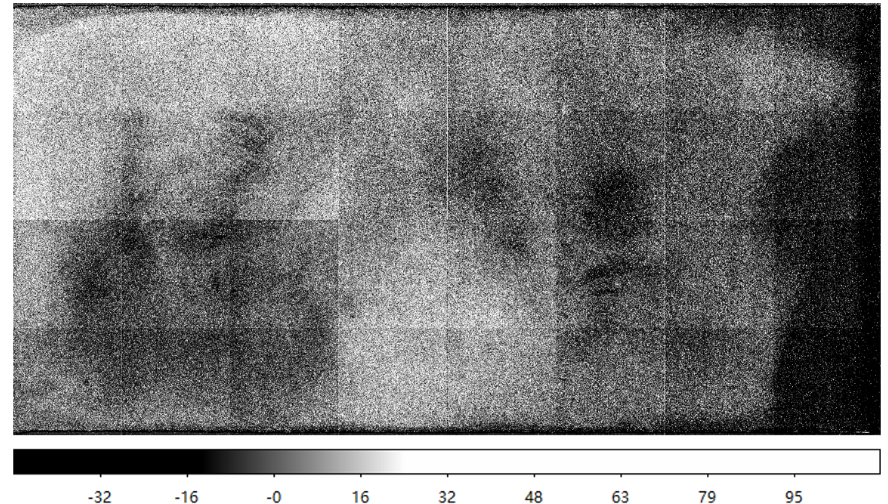
Figure 3: The dark frame generated from observation. The difference between bright and dark regions is obvious.

4.1.3 Flat field correction

During the beginning of the observing season, we took numerous twilight sky images and produced a master flat-field image. The large FOV of AST3 led to a non-uniform large-scale gradient of the twilight images, which varied with the Sun elevation and angular distance from the field. The method of brightness gradient correction was studied in Wei et al. (2014). Two-dimensional fitting was applied to each flat image to correct the brightness gradient. Finally, we median combined the corrected flat images to construct a master flat-field image. After the correction, the mean root-mean-square (RMS) of the master flat was far below 1 per cent.

4.1.4 Cross-talk and stripey noise corrections

Due to the simultaneous CCD readouts, when one amplifier reads a saturated pixel, other amplifiers will be affected. There are significant CCD cross-talk effects in the raw images. As Fig. 4 shows, when one saturated pixel is read in one readout channel, the other 15 channels will have a negative ghost image at the exact position of the saturated pixel presenting as a dark spot. To remove the effect, we initially planned to locate all the saturated pixels, find the position of the related ghost pixels, and add the appropriate negative values back. However, the unsaturated pixels around the saturated ones also have cross-talk effects, making the ghost images hard to locate. So we developed a method to correct the cross-talk effect during the correction for the stripey noise, described below.

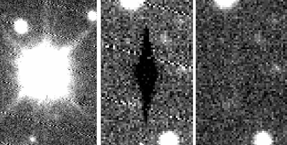
Figure 4: An example of the cross-talk effect in the AST3 raw image. The left panel shows a saturated star in one channel that would cause the cross-talk effect in other channels. The middle panel shows the mirror pixels where the saturated pixels are in another CCD channel. The stripey noise can also be seen in this area. The right panel shows the same image as in the middle panel but after the cross-talk effect and the stripey noise are corrected.

As Fig. 5 shows, the raw images of AST3 in 2016 have shown an unusual kind of stripey noise. After careful investigation, we found that the diagonal stripes were due to electromagnetic interference at 16 kHz caused by a broken ground shield in the cables for the telescope’s DC motor drives. Because this noise lies in exactly the same positions in each of the 16 CCD channels, and is extremely reproducible, for each channel we constructed a filtered image from the other 15 channels by median combining the star-removed images of single channels. By subtracting from each channel the filtered image, we can remove the stripey noise to the point where it is not detectable, as Fig. 5 shows. The pattern of the noise is similar to the cross-talk effect, which also lies at the same position of different readout channels. So, the above method also helped to correct the cross-talk problem.

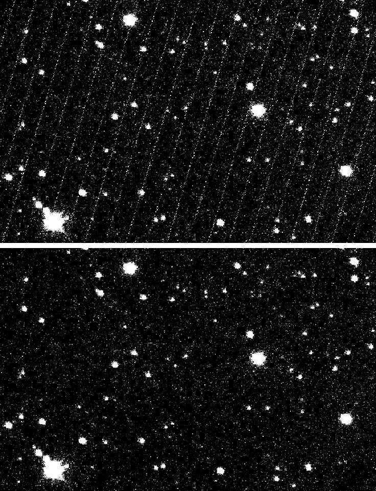
Figure 5: Upper: An example of the stripey noise in the AST3 raw image due to a break in a cable shield. Lower: The same image area but with the noise removed through the method discussed in section 4.1.4.

4.2 Photometry and astrometry

4.2.1 Photometry

We performed aperture photometry using the Source Extractor (Bertin & Arnouts, 1996). Considering the changing full width at half maximum (FWHM) of our images, we used multiple apertures to adapt to the varying image quality. The aperture radii were set to 3, 5, and 7 pixels. Because the median FWHM of our data is 5 pixels, we set the default aperture radius as 5 pixels, or 5″at our pixel scale of 1″/pixel. An additional Kron-like elliptical aperture magnitude MAG_AUTO was adopted for galaxies. Fig. 6 shows the photometric accuracy of two consecutive images by comparing the magnitude differences between them.

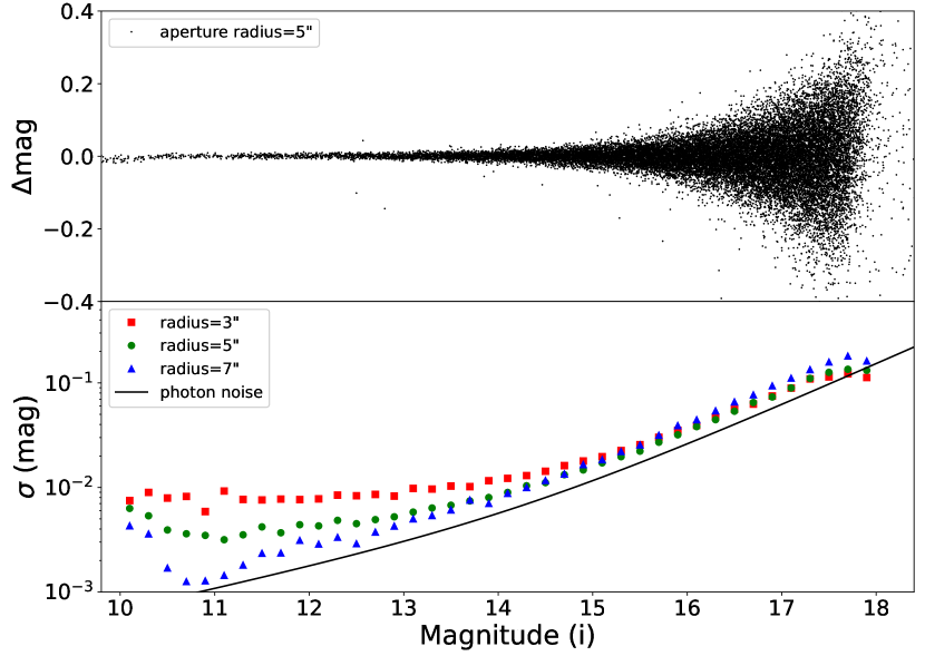
Figure 6: The upper panel presents the magnitude differences between two consecutive exposures b160505.000122 and b160505.000123 as a function of $i$-band magnitude measured with a circular aperture of 3″in radius. The lower panel presents the magnitude RMS calculated in 0.2 magnitude bins. The different colours represent different circular apertures. The solid lines are the expected error from photon noise of 5″radius. The trend of magnitude $\sigma$ changing with aperture goes contrary at different magnitude ends. At the brighter end, the $\sigma$ is lower when the aperture radius is higher. It means for brighter stars larger apertures are appropriate when the photon noise of the star itself is dominant. The stars brighter than 11 magnitudes are saturated and have higher $\sigma$. At the fainter end, the $\sigma$ is lower when the aperture radius is lower. This is because the sky background dominated the noise for fainter stars and a smaller aperture is more suitable. The number of stars is insufficient at the very faint end, thus the $\sigma$ is not real and seems to be smaller than the ideal photon noise.

4.2.2 Astrometry

For astrometry, we used SCAMP to solve the World Coordinate System (Bertin, 2006). We adopted the Position and Proper Motions eXtended catalogue (PPMX) as a reference, which contains 440 sources per deg² with the one-dimensional precision of 40 mas (Röser et al., 2008). As a result, the external precision of our astrometric calibration is 0.1″and the internal precision is 0.06″, in both Right Ascension (RA) and Declination (Dec.).

4.2.3 Flux calibration

We adopted the SkyMapper catalogue as the $i$-band magnitude reference for the flux calibration (Wolf et al., 2018). The SkyMapper Southern Survey is a southern hemispheric survey carried out with the SkyMapper Telescope at Siding Spring Observatory in Australia. It covers an area of 17,200 deg² and the limiting magnitude reaches a depth of roughly 18 magnitudes in $uvgriz$ pass band.

We first chose our best frame of each survey field for absolute calibration. The “best” refers to the images that have the best image quality in one field considering the number of detected sources, background brightness, FWHM, and elongation. Then we calculate the zero point in $i$-band magnitude for calibration. We only chose the stars that are between 11 and 14 magnitudes in the $i$-band for calibration to balance high accuracy with a sufficient number of stars.

After the absolute calibration, we used these calibrated images as references to relatively calibrate the other images of each survey field. However, we found that the zero point changes with position and the cause still requires further investigation. To avoid large field non-uniformity of the zero point, we decide to do the flux calibration in each readout channel.

For the AST3-2 survey, we only have $i$-band data. To investigate the colour term, we compared the AST3-2 $i$-band data with SkyMapper $i$- and $g$-band data as Fig. 7 shows. The colour coefficient is 0.02, much smaller than that for AST3-1 reported by Ma et al. (2018). However, we used a different reference catalogue from AST3-1, which adopted the AAVSO Photometric All-Sky Survey catalogue (APASS; Henden et al. (2016)). Our $i$-band magnitude matches relatively well with the SkyMapper catalogue, but to compare with other catalogues observed in the same band we need to be cautious.

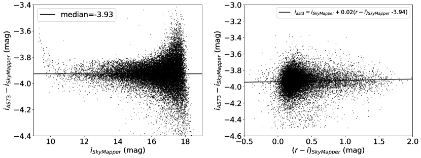
Figure 7: Left panel: The magnitude difference between AST3-2 and SkyMapper in the AST3-2 image b160505.000122. Right panel: The difference between the $i$-band catalogue of SkyMapper and AST3-2 versus the SkyMapper $r-i$ magnitude.

4.3 Data quality

Fig. 8 displays the distributions of data quality, showing the median value of elongation of $\sim$1.17, FWHM of 5″, background of 670 ADU, and limiting magnitude of 17.8 mag. Some issues with tracking stability AST3-2 led to the elongated star profiles. We also see this problem from the range of FWHM, which varies from 3 to 7 arcseconds. Another cause of the wide FWHM distribution was the changing tube seeing. In the extremely cold and high relative humidity conditions at Dome A, there can be frost on the first surface of the optical system that reduces the transmission and changes the point-spread function through scattering. As described in section 2, a heater and a blower were used to prevent the frosting problem, and the tube seeing would be unstable when they were working. As a result, the limiting magnitude is not as good as that of the first AST3 telescope AST3-1 (Ma et al., 2018).

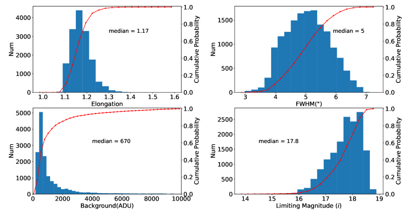
Figure 8: The statistics of the star elongation, FWHM, sky background, and limiting magnitude of the data, which had median values of 1.17, 5″, 670 ADU, and 17.8 mag, respectively.

5 Stellar Variability and Statistics

5.1 Time series

Images with poor quality were first excluded to ensure the quality of the light curves. Such images could be due to heavy frost, or doubling of stars images from tracking problems. We also excluded images with a background brightness larger than 10,000 ADU, median FWHM larger than 8″, fewer than 2000 stars, and median elongations larger than 2. In this way, we excluded about 30 per cent of the images. We then cross-matched the targets in each field and obtained light curves. Finally, an additional outlier elimination was performed to remove the false targets with obvious anomalous magnitudes and FWHMs. Fig. 9 shows a typical light curve dispersion with an aperture radius of 5″.

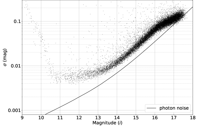
Figure 9: The light curve rms as a function of magnitude. Each data point represents a light curve from the region b160505.000122.

5.2 Period search

On average, we observed each survey field 30 times during the year. Some of the targets might not be detected in some images due to poor image quality etc. Thus, together with the image selections in section 5.1, for each target, the total number of epochs could be less than 30. To analyse the stellar variability with enough detection and better image quality, we restricted ourselves to sky fields with more than 30 observations. There are about one-third of the observations were exposed 3 times continuously, originally for image combination. Due to the tracking problem discussed in section 4.3 and section 5.1, some of the multi-images would be excluded in the image selections and we tend not to combine them. For the remaining multi-images, we did not count them as individual observations, but we used them as independent data points in light curve analysis. Then, we rejected the targets that were only detected in less than 50 per cent of the images. Finally, in the period analysis, we chose the light curves with a significant variability of more than 2.5$\sigma$.

For our survey data, the sampling in the light curves with time is not uniform and thus we used the Lomb-Scargle (LS) method for period search (Lomb, 1976; Scargle, 1982). Light curves with a signal-to-noise ratio (SNR) larger than 5 are considered eligible candidates. Then we cross-matched the candidate light curves with the International Variable Star Index (VSX; Watson et al. 2006) and found 3,551 known variables. For candidates that were not in the VSX catalogue, we visually inspected whether their periodicities were significant or not. For candidates that were significantly variable and periodic, we then checked whether it was a false signal. For example, Fig.10 shows a comparison of the true and false EA-type variable candidates. The former is an EA-type variable candidate included in the VSX catalogue. The latter shows a similar light curve pattern but turned out to be a false signal affected by an outlier. We manually excluded these kinds of false signals and we take the true ones as variable candidates. In total, we found 70 new variables.

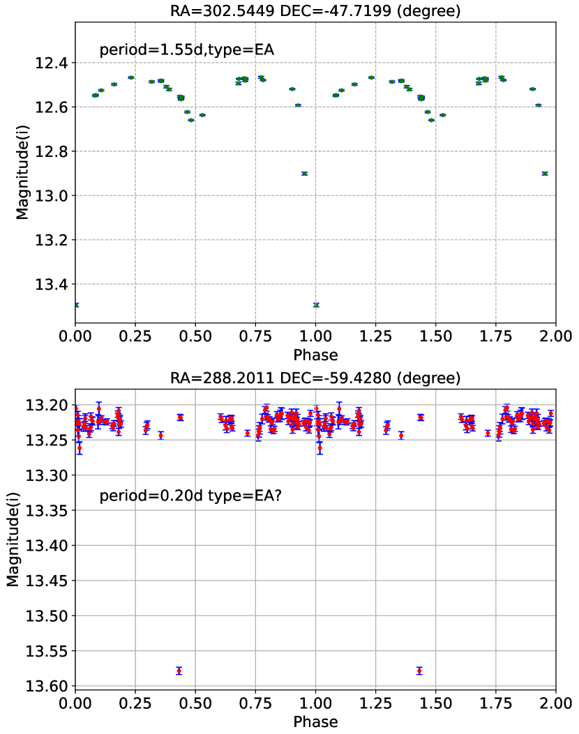
Figure 10: Upper: An example light curve of an EA-type variable star folded in 2 phases. Lower: An example false signal showing an EA-type variable pattern.

5.3 New variables

For the newly discovered variable candidates, we tried to visually classify them into different classes by their periods, amplitudes, and light curve patterns. We also obtained their effective temperature, surface gravity, and metallicity from StarHorse (Anders et al., 2019) to help the classification. Moreover, we obtained their B-V from the UCAC4 (Zacharias et al., 2013), APASS9 (Henden et al., 2016), NOMAD (Zacharias et al., 2004), and SPM4.0 (Girard et al., 2011) catalogues. However, due to insufficient observations, it was still hard to classify them such as the example in section 5.2. The insufficient observations at the minimum luminosity make it hard to classify. Many under-sampled candidates were excluded from the candidate list if they were not a known variable.

For this reason, we were only able to classify the candidates into 5 different classes. There are 17 candidates classified as long-period variables (LPV) either because they were observed in less than one period or because we could hardly distinguish one periodic signal from its light curve. We found 5 candidates with Cepheid-like signals and we classified them as pulsating stars (PUL). We found 4 candidates as eclipsing binary (EC) candidates by their periods and patterns. Of the remaining candidates, 24 of them have small amplitudes ($<0.1$) and long periods (a few days to a dozen days), and they are likely to be rotational variables (ROT). The final 20 candidates have periods shorter than 2 days and some of their periods are even shorter than 0.2 days. Most of these candidates have strange phase diagram patterns and we are not sure whether they are real or a result of a lack of data points. Under this circumstance, we classified them as possible rotational variables (pROT). Fig. 11 shows the typical phased or time-series light curves of each class.

As mentioned in section 5.2, when we try to classify the light curves, we only consider the ones with 30 epochs or more to ensure there are enough observations for a reliable period. We can confirm some of them that have obvious and distinctive light curve patterns. But for many variables that met the 30 epoch threshold, the absence of critical data points in the light curves might lead to a false period, and an incorrect pattern in their phase diagrams. In such cases we erred on the side of not claiming them as newly discovered variables.

We cross-matched our variable candidates with the VSX catalogue version 2022-10-31. Interestingly, we initially used an earlier version of the VSX catalogue and our count of new candidates was 126; 56 of these were listed in the latest version, which gave us the opportunity of comparing our classifications with VSX. The classifications agreed well, with disagreements mainly with LPVs and ECs. Some stars were identified as rotational variables in the VSX that we classified as LPVs because we have relatively time coverage and we considered all the light curves with less than one period as LPVs. As for the ECs in VSX, we classified some of them as ROTs or pROTs since we did not have enough critical data points to confirm them.

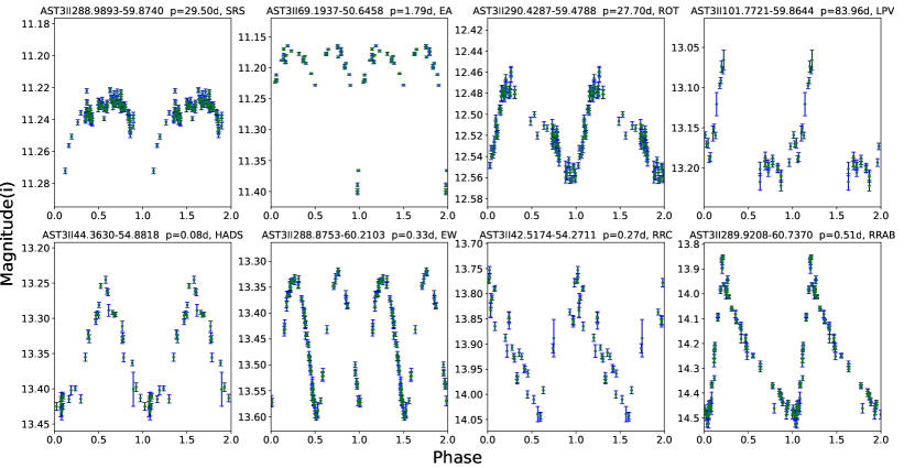
Figure 11: Example light curves of the variables in different classes folded in 2 phases. Periods and types are marked on the light curves.

6 Data Availability

The AST3-2 data is available through the Chinese Astronomical Data Center (CADC)^, . The data contains an $i$-band catalogue, a light curve catalogue, and preprocessed images.

The $i$-band catalogue contains over 7 million sources with a median limiting magnitude of 17.8 mag. For objects with multiple observations, we adopted their median positions and median magnitudes. Table 1 shows the Database Schema of the catalogue.

Table 2 details the information in the light curve catalogue. The light curves are presented as time series and the catalogue contains information from every observation after quality filtering. The periodic variables discussed in this work are also presented and listed in Appendix A.

There are also 22576 images in the format of Flexible Image Transport System (FITS) presented in the data set. These are the preprocessed FITS images discussed in section 4 with observing information such as date, exposure time, and WCS coordinates.

Table 1: AST3-2 survey catalogue Table Schema

Column Name	Description
ID	Source index
RA	Right Ascension in J2000 (deg)
Dec.	Declination in J2000 (deg)
MAG	Median aperture magnitudes (mag)
MAGERR	Standard deviation of magnitudes (mag)
COUNT	Number of observations

Table 2: AST3-2 light curve catalogue Table Schema

Column Name	Description
DATE	The beginning time of observation in
	ISO time
MJD	The beginning time of observation in
	Modified Julian date
X	Windowed X position in CCD (pixel)
Y	Windowed Y position in CCD (pixel)
RA	Right Ascension in J2000 (deg)
DEC	Declination in J2000 (deg)
MAG	Aperture magnitudes in 5″radius (mag)
MAGERR	Aperture magnitude errors in 5″radius
	(mag)
FLUX	Flux (ADU)
FLUXERR	Flux error (ADU)
MAG$\_$AUTO	Magnitude in Kron aperture (mag)
MAGERR$\_$AUTO	Magnitude error in Kron aperture (mag)
BACKGROUND	Background brightness (ADU)
FWHM	Full width at half-maximum in Gaussian
	profile (pixel)
ELONGATION	Ratio of semi-major to semi-minor axis
A	Semimajor axis length (pixel)
B	Semiminor axis length (pixel)
THETA	Position angle of semimajor axis (degrees
	east from north)
MAG$\_$3	Aperture magnitudes in 3″radius (mag)
MAGERR$\_$3	Aperture magnitude errors in 3″radius
	(mag)
MAG$\_$7	Aperture magnitudes in 7″radius (mag)
MAGERR$\_$7	Aperture magnitude errors in 7″radius
	(mag)

7 Summary

The second AST3 telescope AST3-2 was deployed at Dome A, Antarctica in 2015. In 2016, it worked fully automatically on a sky survey for SNae and semi-automatically on an exo-planet search. In this work, we report on the 2016 SN survey data observed between Mar. 23 and May 16. We surveyed 2200 deg² fields with about 30 visits each in a cadence of a half to a few days. After the raw data was retrieved, we preprocessed the data, performed aperture photometry, calibrated the magnitudes, obtained the light curves of the 565 sky fields, and briefly studied the variability of the light curves. In this paper, we present the data release of the photometric data from the AST3-2 SN survey in 2016. It consists of 22000 scientific images, 7 million sources brighter than $i\sim$18 with photometry, astrometry, and light curves.

The 5$\sigma$ limiting magnitude of this dataset is 17.8 mag with 4 mmag precision in the light curves of bright stars. The median FWHM, elongation, and background brightness are 5.0″, 1.17, and 670 ADU, respectively. We found 70 new variable candidates out of $\sim$ 3,500 variable stars. We check the stellar properties from surveys such as StarHorse to help us classify these variables into 5 types.

Appendix A The Light curves of New Candidates

Fig.12 shows the phased new variable candidates, and Table 3 shows the list of them.

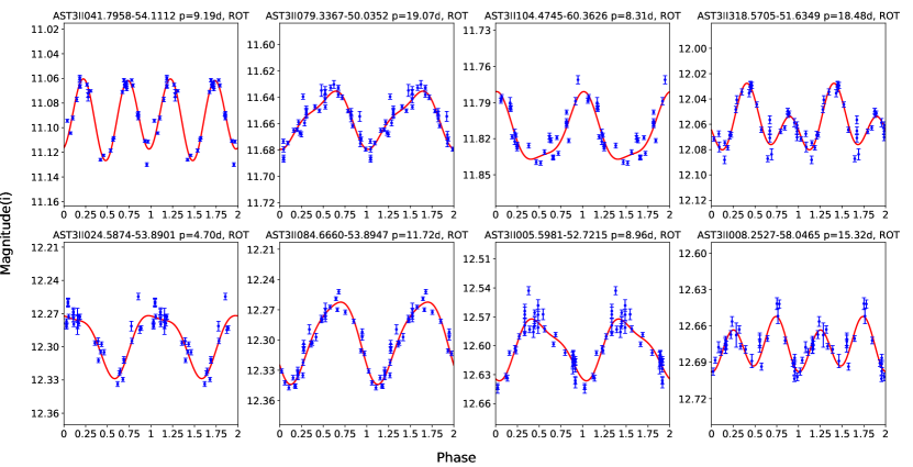
Figure 12: Light curves of the new candidates in different classes folded in 2 phases except the LPVs show no apparent periods and are in the form of time series. The dots with error bars are observed data and the red curve is the fitted line. Periods and types are marked on the light curves. The pulsating stars are marked as PUL and the possible rotational variables are marked as pROT.

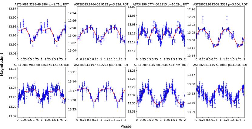
Figure 13: continued

Light curves of the new candidates in different classes folded in 2 phases except the LPVs show no apparent periods and are in the form of time series. The dots with error bars are observed data and the red curve is the fitted line. Periods and types are marked on the light curves. The pulsating stars are marked as PUL and the possible rotational variables are marked as pROT.

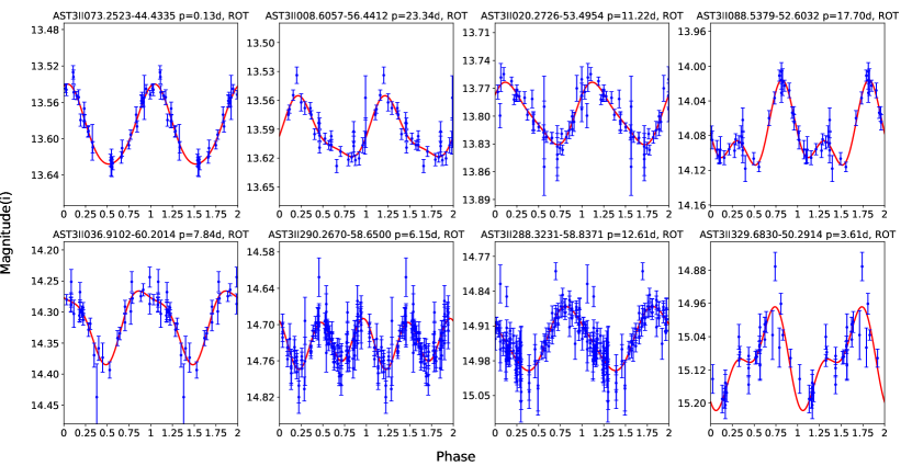
Figure 14: continued

Light curves of the new candidates in different classes folded in 2 phases except the LPVs show no apparent periods and are in the form of time series. The dots with error bars are observed data and the red curve is the fitted line. Periods and types are marked on the light curves. The pulsating stars are marked as PUL and the possible rotational variables are marked as pROT.

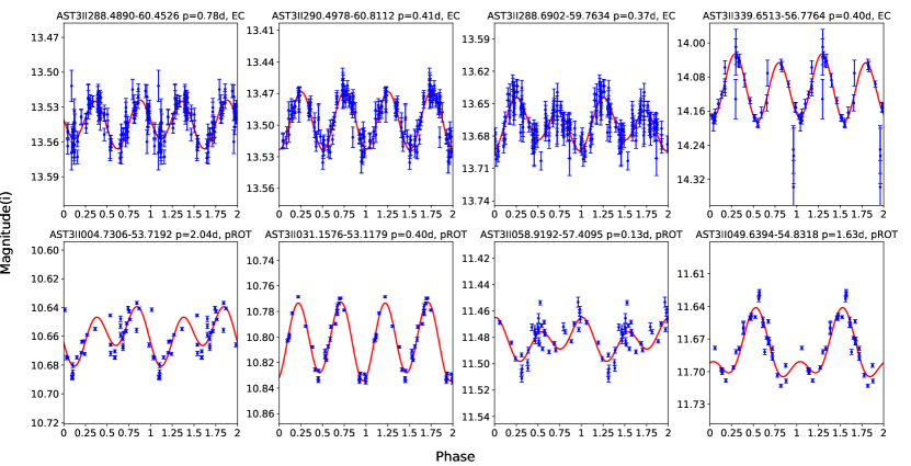
Figure 15: continued

Light curves of the new candidates in different classes folded in 2 phases except the LPVs show no apparent periods and are in the form of time series. The dots with error bars are observed data and the red curve is the fitted line. Periods and types are marked on the light curves. The pulsating stars are marked as PUL and the possible rotational variables are marked as pROT.

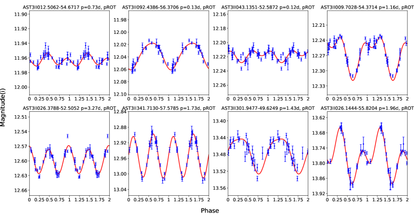
Figure 16: continued

Light curves of the new candidates in different classes folded in 2 phases except the LPVs show no apparent periods and are in the form of time series. The dots with error bars are observed data and the red curve is the fitted line. Periods and types are marked on the light curves. The pulsating stars are marked as PUL and the possible rotational variables are marked as pROT.

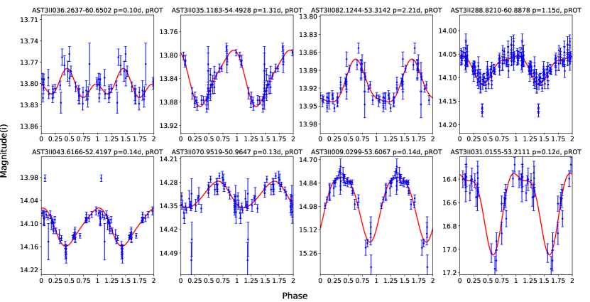
Figure 17: continued

Light curves of the new candidates in different classes folded in 2 phases except the LPVs show no apparent periods and are in the form of time series. The dots with error bars are observed data and the red curve is the fitted line. Periods and types are marked on the light curves. The pulsating stars are marked as PUL and the possible rotational variables are marked as pROT.

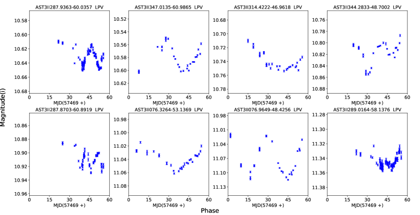
Figure 18: continued

Light curves of the new candidates in different classes folded in 2 phases except the LPVs show no apparent periods and are in the form of time series. The dots with error bars are observed data and the red curve is the fitted line. Periods and types are marked on the light curves. The pulsating stars are marked as PUL and the possible rotational variables are marked as pROT.

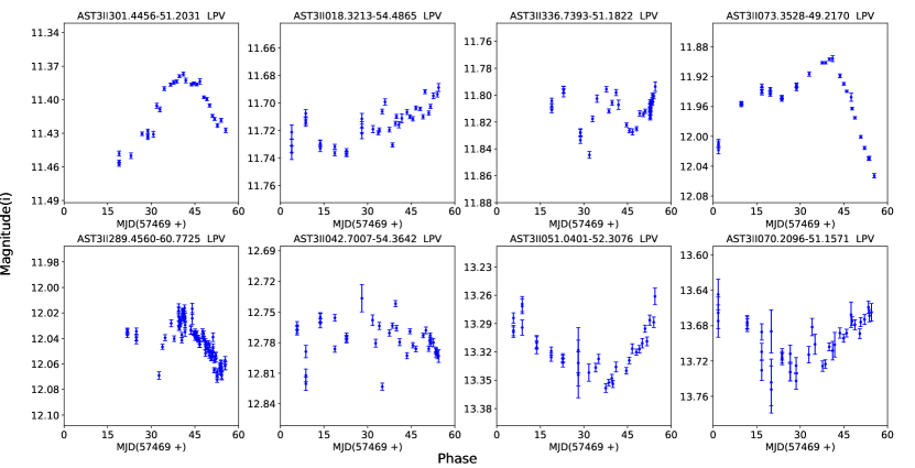
Figure 19: continued

Light curves of the new candidates in different classes folded in 2 phases except the LPVs show no apparent periods and are in the form of time series. The dots with error bars are observed data and the red curve is the fitted line. Periods and types are marked on the light curves. The pulsating stars are marked as PUL and the possible rotational variables are marked as pROT.

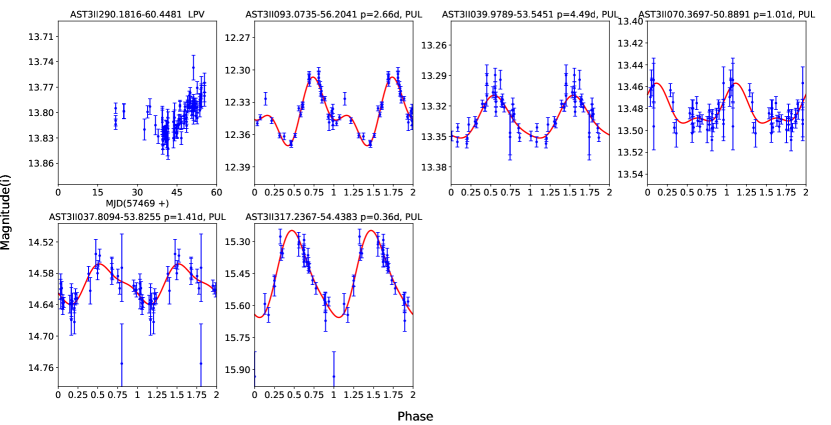
Figure 20: continued

Light curves of the new candidates in different classes folded in 2 phases except the LPVs show no apparent periods and are in the form of time series. The dots with error bars are observed data and the red curve is the fitted line. Periods and types are marked on the light curves. The pulsating stars are marked as PUL and the possible rotational variables are marked as pROT.

Table 3: The list of new variable candidates.

Namea	Magnitudeb	Period	Amplitude	Type	B-V	B-V ref.	Teffc	logg	[Fe/H]
	(mag)	(days)	(mag)		(mag)		(K)	([cm/s2])
AST3II004.7306-53.7192	10.7	2.04	0.05	ROT?	0.22	UCAC4d	7714	3.90	-0.38
AST3II031.1576-53.1179	10.8	0.40	0.07	ROT?	0.76	UCAC4	5888	4.09	-0.18
AST3II049.6394-54.8318	11.7	1.63	0.09	ROT?	0.52	UCAC4	5489	3.68	-0.81
AST3II058.9192-57.4095	11.5	0.13	0.06	ROT?	0.85	UCAC4	6201	4.49	-0.78
AST3II012.5062-54.6717	12	0.73	0.03	ROT?	1.21	UCAC4	5210	4.48	0.27
AST3II092.4386-56.3706	12	0.13	0.05	ROT?	0.79	UCAC4	5703	4.33	-0.02
AST3II043.1351-52.5872	12.2	0.12	0.03	ROT?	0.53	UCAC4	6257	4.30	-0.19
AST3II009.7028-54.3714	12.3	1.16	0.08	ROT?	0.44	UCAC4	6039	3.94	-0.79
AST3II026.3788-52.5052	12.6	3.27	0.08	ROT?	1.55	APASS9e	3141	4.70	0.06
AST3II341.7130-57.5785	12.9	1.73	0.13	ROT?	0.90	UCAC4	5546	4.50	-0.10
AST3II301.9477-49.6249	13.5	1.43	0.11	ROT?	1.28	NOMADf	3767	4.64	0.21
AST3II026.1444-55.8204	13.8	1.96	0.24	ROT?	0.88	UCAC4	5177	3.45	-0.53
AST3II036.2637-60.6502	13.8	0.10	0.07	ROT?	0.86	UCAC4	5137	4.59	-0.13
AST3II035.1183-54.4928	13.9	1.31	0.11	ROT?	0.85	UCAC4	5329	4.57	-0.22
AST3II082.1244-53.3142	13.9	2.21	0.10	ROT?	1.30	UCAC4	5077	4.51	0.19
AST3II043.6166-52.4197	14.1	0.14	0.21	ROT?	0.92	UCAC4	5826	4.32	-0.12
AST3II288.8210-60.8878	14.1	1.15	0.15	ROT?	1.44	UCAC4	4933	4.60	0.00
AST3II070.9519-50.9647	14.3	0.13	0.25	ROT?	1.02	UCAC4	5433	4.41	0.12
AST3II009.0299-53.6067	14.8	0.14	0.60	ROT?	0.75	NOMAD	5482	4.40	0.12
AST3II031.0155-53.2111	16.5	0.12	0.89	ROT?	1.71	NOMAD	4145	4.62	0.40

Table 4: continued

The list of new variable candidates. Name^a Mag^b P Amp. Type B-V B-V ref. Teff^c logg [Fe/H] (mag) (days) (mag) (mag) (K) ([cm/s²]) AST3II290.4978-60.8112 13.5 0.41 0.08 EC 0.60 UCAC4 6397 3.97 -0.29 AST3II288.4890-60.4526 13.5 0.78 0.06 EC 0.43 UCAC4 6349 2.68 -1.38 AST3II288.6902-59.7634 13.7 0.37 0.07 EC 0.85 UCAC4 5801 4.13 0.00 AST3II339.6513-56.7764 14.1 0.40 0.33 EC 0.28 UCAC4 6630 4.08 -0.49 AST3II287.9363-60.0357 10.6 23.72 0.04 LPV 1.07 UCAC4 4480 1.14 -1.40 AST3II314.4222-46.9618 10.7 200 0.04 LPV 0.30 UCAC4 8526 4.25 -0.15 AST3II347.0135-60.9865 10.6 55.93 0.05 LPV 0.89 UCAC4 5023 3.55 -0.11 AST3II344.2833-48.7002 10.8 34.12 0.07 LPV 1.54 UCAC4 3728 0.79 -0.21 AST3II076.3264-53.1369 11 54.39 0.05 LPV 0.80 UCAC4 5410 3.30 -0.40 AST3II287.8703-60.8919 10.9 16.93 0.05 LPV 1.29 UCAC4 4611 2.41 0.10 AST3II076.9649-48.4256 11.1 28.69 0.1 LPV 1.10 UCAC4 4831 2.30 -0.64 AST3II289.0164-58.1376 11.3 15.52 0.03 LPV 1.53 UCAC4 4007 0.93 -0.58 AST3II301.4456-51.2031 11.4 46.78 0.08 LPV 0.78 NOMAD 4115 1.28 -0.39 AST3II018.3213-54.4865 11.7 62.96 0.05 LPV 1.67 APASS9 3018 4.94 0.24 AST3II336.7393-51.1822 11.8 16.35 0.05 LPV 0.96 UCAC4 5033 4.65 -0.51 AST3II073.3528-49.2170 11.9 65.51 0.16 LPV 0.92 UCAC4 4805 2.58 -0.47 AST3II289.4560-60.7725 12 23.72 0.06 LPV 0.82 UCAC4 5156 3.20 -0.49 AST3II042.7007-54.3642 12.8 98.65 0.09 LPV 0.59 SPM4.0^g 6359 4.34 -0.41 AST3II051.0401-52.3076 13.3 123.73 0.10 LPV 1.53 UCAC4 4372 0.81 -1.55 AST3II070.2096-51.1571 13.7 200 0.11 LPV 1.77 UCAC4 * * * AST3II290.1816-60.4481 13.8 43.79 0.10 LPV 0.91 UCAC4 5153 3.45 -0.49 AST3II093.0735-56.2041 12.3 2.66 0.07 PUL 0.24 UCAC4 5560 3.46 -1.42 AST3II039.9789-53.5451 13.3 4.49 0.07 PUL 0.77 UCAC4 5880 4.25 -0.14 AST3II070.3697-50.8891 13.5 1.01 0.05 PUL 0.62 UCAC4 10089 4.40 -0.65 AST3II037.8094-53.8255 14.6 1.41 0.21 PUL 1.33 UCAC4 4947 4.65 -0.48 AST3II317.2367-54.4383 15.4 0.36 0.66 PUL 0.27 UCAC4 6880 3.83 -0.79 AST3II041.7958-54.1112 11.1 9.19 0.07 ROT 0.50 UCAC4 8240 4.17 0.05 AST3II079.3367-50.0352 11.7 19.07 0.06 ROT 0.90 UCAC4 5326 4.56 -0.14 AST3II104.4745-60.3626 11.8 8.31 0.07 ROT 1.22 UCAC4 5569 4.56 -0.32 AST3II318.5705-51.6349 12.1 18.48 0.06 ROT 1.06 UCAC4 4817 2.53 -0.32 AST3II024.5874-53.8901 12.3 4.7 0.08 ROT 1.55 APASS9 3272 4.84 0.09 AST3II084.6660-53.8947 12.3 11.72 0.10 ROT 0.88 UCAC4 5543 3.89 -0.37 AST3II005.5981-52.7215 12.6 8.96 0.10 ROT 0.77 UCAC4 5385 3.75 -0.35 AST3II008.2527-58.0465 12.7 15.32 0.06 ROT 0.71 UCAC4 5427 3.53 -0.85 AST3II081.3298-46.8904 12.9 1.71 0.08 ROT 0.64 UCAC4 6093 4.03 -0.46 AST3II025.8764-53.9192 13 3.83 0.04 ROT 0.72 UCAC4 5562 4.41 -0.27 AST3II062.9212-52.3332 13.1 5.76 0.11 ROT 1.54 UCAC4 3221 4.78 0.44 AST3II084.1197-53.2223 13.2 7.42 0.07 ROT 0.76 UCAC4 5156 3.53 -0.36 AST3II290.0774-60.2915 13.1 10.29 0.08 ROT 1.14 UCAC4 6085 4.28 -0.38 AST3II288.7966-60.6563 13.2 12.15 0.07 ROT 1.10 UCAC4 4723 2.53 -0.22 AST3II289.3107-60.9644 13.3 4.79 0.09 ROT 0.90 UCAC4 5185 3.49 -0.39 AST3II073.2523-44.4335 13.6 0.13 0.11 ROT 0.58 UCAC4 6146 4.30 -0.31 AST3II008.6057-56.4412 13.6 23.34 0.09 ROT 0.98 UCAC4 4962 2.94 -0.48 AST3II288.1145-59.8068 13.5 3.08 0.07 ROT 0.26 NOMAD 4877 4.59 0.12 AST3II020.2726-53.4954 13.8 11.22 0.10 ROT 0.92 UCAC4 5131 3.70 -0.29 AST3II088.5379-52.6032 14.1 17.70 0.11 ROT 0.97 UCAC4 5072 3.42 -0.31 AST3II036.9102-60.2014 14.3 7.84 0.19 ROT 0.72 UCAC4 5488 3.65 -0.90 AST3II290.2670-58.6500 14.7 6.15 0.20 ROT 1.62 UCAC4 4004 4.69 -0.29 AST3II288.3231-58.8371 14.9 12.61 0.26 ROT 0.74 NOMAD 4942 3.36 -0.18 AST3II329.6830-50.2914 15.1 3.61 0.33 ROT 0.77 NOMAD 5193 3.28 -0.68

References

- Anders et al. (2019) Anders F., et al., 2019, A&A, 628, A94
- Ashley (2013) Ashley M. C. B., 2013, in Burton M. G., Cui X., Tothill N. F. H., eds, Proceedings of the International Astronomical Union Vol. 288, Astrophysics from Antarctica. pp 15–24, doi:10.1017/S1743921312016614
- Ashley et al. (2010) Ashley M. C. B., Bonner C. S., Everett J. R., Lawrence J. S., Luong-Van D., McDaid S., McLaren C., Storey J. W. V., 2010, in McLean I. S., Ramsay S. K., Takami H., eds, Society of Photo-Optical Instrumentation Engineers (SPIE) Conference Series Vol. 7735, Ground-based and Airborne Instrumentation for Astronomy III. p. 773540, doi:10.1117/12.857853
- Bellm et al. (2019) Bellm E. C., et al., 2019, PASP, 131, 018002
- Bertin (2006) Bertin E., 2006, in Gabriel C., Arviset C., Ponz D., Enrique S., eds, Astronomical Society of the Pacific Conference Series Vol. 351, Astronomical Data Analysis Software and Systems XV. p. 112
- Bertin & Arnouts (1996) Bertin E., Arnouts S., 1996, A&AS, 117, 393
- Bonner et al. (2010) Bonner C. S., et al., 2010, PASP, 122, 1122
- Burton et al. (2016) Burton M. G., et al., 2016, Publ. Astron. Soc. Australia, 33, e047
- Cui et al. (2008) Cui X., Yuan X., Gong X., 2008, in Stepp L. M., Gilmozzi R., eds, Society of Photo-Optical Instrumentation Engineers (SPIE) Conference Series Vol. 7012, Ground-based and Airborne Telescopes II. p. 70122D, doi:10.1117/12.789458
- Girard et al. (2011) Girard T. M., et al., 2011, AJ, 142, 15
- Henden et al. (2016) Henden A. A., Templeton M., Terrell D., Smith T. C., Levine S., Welch D., 2016, VizieR Online Data Catalog, p. II/336
- Hill & Salinari (2000) Hill J. M., Salinari P., 2000, in Sebring T. A., Andersen T., eds, Society of Photo-Optical Instrumentation Engineers (SPIE) Conference Series Vol. 4004, Telescope Structures, Enclosures, Controls, Assembly/Integration/Validation, and Commissioning. pp 36–46, doi:10.1117/12.393947
- Hu et al. (2014) Hu Y., et al., 2014, PASP, 126, 868
- Hu et al. (2016a) Hu Y., Shang Z., Ma B., Hu K., 2016a, in Chiozzi G., Guzman J. C., eds, Society of Photo-Optical Instrumentation Engineers (SPIE) Conference Series Vol. 9913, Software and Cyberinfrastructure for Astronomy IV. p. 99130M, doi:10.1117/12.2231851
- Hu et al. (2016b) Hu L., et al., 2016b, Transient Name Server Discovery Report, 2016-338, 1
- Hu et al. (2017) Hu L., et al., 2017, GRB Coordinates Network, 21883, 1
- Hu et al. (2019) Hu Y., et al., 2019, PASP, 131, 015001
- Ivezic et al. (2008) Ivezic Z., et al., 2008, Serbian Astronomical Journal, 176, 1
- Li et al. (2016) Li Y., et al., 2016, Publ. Astron. Soc. Australia, 33, e008
- Liang et al. (2016) Liang E.-S., et al., 2016, AJ, 152, 168
- Liang et al. (2020) Liang E.-S., et al., 2020, AJ, 159, 201
- Liu et al. (2018) Liu Q., Wei P., Shang Z.-H., Ma B., Hu Y., 2018, Research in Astronomy and Astrophysics, 18, 005
- Lomb (1976) Lomb N. R., 1976, Ap&SS, 39, 447
- Ma et al. (2012) Ma B., Shang Z., Wang L., Boggs K., Hu Y., Liu Q., Song Q., Xue S., 2012, in McLean I. S., Ramsay S. K., Takami H., eds, Society of Photo-Optical Instrumentation Engineers (SPIE) Conference Series Vol. 8446, Ground-based and Airborne Instrumentation for Astronomy IV. p. 84466R, doi:10.1117/12.927098
- Ma et al. (2014a) Ma B., et al., 2014a, Central Bureau Electronic Telegrams, 3796, 1
- Ma et al. (2014b) Ma B., Wei P., Shang Z., Wang L., Wang X., 2014b, The Astronomer’s Telegram, 5794, 1
- Ma et al. (2014c) Ma B., Shang Z., Hu Y., Liu Q., Wang L., Wei P., 2014c, in Holland A. D., Beletic J., eds, Society of Photo-Optical Instrumentation Engineers (SPIE) Conference Series Vol. 9154, High Energy, Optical, and Infrared Detectors for Astronomy VI. p. 91541T (arXiv:1407.8279), doi:10.1117/12.2055416
- Ma et al. (2014d) Ma B., Shang Z., Wang L., Hu Y., Liu Q., Wei P., 2014d, in Holland A. D., Beletic J., eds, Society of Photo-Optical Instrumentation Engineers (SPIE) Conference Series Vol. 9154, High Energy, Optical, and Infrared Detectors for Astronomy VI. p. 91541U (arXiv:1407.8280), doi:10.1117/12.2055430
- Ma et al. (2016) Ma B., Hu Y., Shang Z., Wang L., 2016, The Astronomer’s Telegram, 9033, 1
- Ma et al. (2018) Ma B., et al., 2018, MNRAS, 479, 111
- Ma et al. (2020a) Ma B., et al., 2020a, MNRAS, 496, 2768
- Ma et al. (2020b) Ma B., et al., 2020b, Nature, 583, 771
- Oelkers et al. (2016) Oelkers R. J., et al., 2016, AJ, 151, 166
- Pollacco et al. (2006) Pollacco D. L., et al., 2006, PASP, 118, 1407
- Ricker et al. (2009) Ricker G. R., et al., 2009, in American Astronomical Society Meeting Abstracts #213. p. 403.01
- Röser et al. (2008) Röser S., Schilbach E., Schwan H., Kharchenko N. V., Piskunov A. E., Scholz R. D., 2008, A&A, 488, 401
- Scargle (1982) Scargle J. D., 1982, ApJ, 263, 835
- Shang (2020) Shang Z., 2020, Research in Astronomy and Astrophysics, 20, 168
- Shang et al. (2012) Shang Z., et al., 2012, in Peck A. B., Seaman R. L., Comeron F., eds, Society of Photo-Optical Instrumentation Engineers (SPIE) Conference Series Vol. 8448, Observatory Operations: Strategies, Processes, and Systems IV. p. 844826, doi:10.1117/12.925600
- Shang et al. (2016) Shang Z., Hu Y., Ma B., Hu K., Ashley M. C. B., Wang L., Yuan X., 2016, in Peck A. B., Seaman R. L., Benn C. R., eds, Society of Photo-Optical Instrumentation Engineers (SPIE) Conference Series Vol. 9910, Observatory Operations: Strategies, Processes, and Systems VI. p. 991023, doi:10.1117/12.2231274
- Storey (2005) Storey J. W. V., 2005, Antarctic Science, 17, 555
- Storey (2007) Storey J. W. V., 2007, Chinese Astron. Astrophys., 31, 98
- Wang et al. (2011) Wang L., et al., 2011, AJ, 142, 155
- Wang et al. (2017a) Wang L., et al., 2017a, AJ, 153, 104
- Wang et al. (2017b) Wang L., et al., 2017b, Transient Name Server Discovery Report, 2017-724, 1
- Watson et al. (2006) Watson C. L., Henden A. A., Price A., 2006, Society for Astronomical Sciences Annual Symposium, 25, 47
- Wei et al. (2014) Wei P., Shang Z., Ma B., Zhao C., Hu Y., Liu Q., 2014, in Peck A. B., Benn C. R., Seaman R. L., eds, Society of Photo-Optical Instrumentation Engineers (SPIE) Conference Series Vol. 9149, Observatory Operations: Strategies, Processes, and Systems V. p. 91492H (arXiv:1407.8283), doi:10.1117/12.2055459
- Wolf et al. (2018) Wolf C., et al., 2018, Publ. Astron. Soc. Australia, 35, e010
- Yang et al. (2015) Yang M., et al., 2015, ApJS, 217, 28
- Yang et al. (2017) Yang Y., et al., 2017, AJ, 154, 6
- Yang et al. (2021) Yang X., et al., 2021, MNRAS, 501, 3614
- Yuan & Su (2012) Yuan X., Su D.-q., 2012, MNRAS, 424, 23
- Yuan et al. (2008) Yuan X., et al., 2008, in Stepp L. M., Gilmozzi R., eds, Society of Photo-Optical Instrumentation Engineers (SPIE) Conference Series Vol. 7012, Ground-based and Airborne Telescopes II. p. 70124G, doi:10.1117/12.788748
- Yuan et al. (2010) Yuan X., et al., 2010, in Stepp L. M., Gilmozzi R., Hall H. J., eds, Society of Photo-Optical Instrumentation Engineers (SPIE) Conference Series Vol. 7733, Ground-based and Airborne Telescopes III. p. 77331V, doi:10.1117/12.856671
- Yuan et al. (2014) Yuan X., et al., 2014, in Stepp L. M., Gilmozzi R., Hall H. J., eds, Society of Photo-Optical Instrumentation Engineers (SPIE) Conference Series Vol. 9145, Ground-based and Airborne Telescopes V. p. 91450F, doi:10.1117/12.2055624
- Zacharias et al. (2004) Zacharias N., Monet D. G., Levine S. E., Urban S. E., Gaume R., Wycoff G. L., 2004, in American Astronomical Society Meeting Abstracts. p. 48.15
- Zacharias et al. (2013) Zacharias N., Finch C. T., Girard T. M., Henden A., Bartlett J. L., Monet D. G., Zacharias M. I., 2013, AJ, 145, 44
- Zhang et al. (2019a) Zhang H., et al., 2019a, ApJS, 240, 16
- Zhang et al. (2019b) Zhang H., et al., 2019b, ApJS, 240, 17
- Zhou et al. (2010) Zhou X., et al., 2010, PASP, 122, 347
- Zong et al. (2015) Zong W., et al., 2015, AJ, 149, 84
- Zou et al. (2010) Zou H., et al., 2010, AJ, 140, 602