Movable-Antenna Enhanced Multiuser Communication via Antenna Position Optimization

Abstract

Movable antenna (MA) is a promising technology to improve wireless communication performance by varying the antenna position in a given finite area at the transceivers to create more favorable channel conditions. In this paper, we investigate the MA-enhanced multiple-access channel (MAC) for the uplink transmission from multiple users each equipped with a single MA to a base station (BS) with a fixed-position antenna (FPA) array. A field-response based channel model is used to characterize the multi-path channel between the antenna array of the BS and each user’s MA with a flexible position. To evaluate the MAC performance gain provided by MAs, we formulate an optimization problem for minimizing the total transmit power of users, subject to a minimum-achievable-rate requirement for each user, where the positions of MAs and the transmit powers of users, as well as the receive combining matrix at the BS are jointly optimized. To solve this non-convex optimization problem involving intricately coupled variables, we develop two algorithms based on zero-forcing (ZF) and minimum mean square error (MMSE) combining methods, respectively. Specifically, for each algorithm, the combining matrix of the BS and the total transmit power of users are expressed as a function of the MAs’ position vectors, which are then optimized by using the gradient descent method in an iterative manner. It is shown that the proposed ZF-based and MMSE-based algorithms can converge to high-quality suboptimal solutions with low computational complexities. Simulation results demonstrate that the proposed solutions for MA-enhanced multiple access systems can significantly decrease the total transmit power of users as compared to conventional FPA systems under both perfect and imperfect field-response information.

I Introduction

With advances in the multiple-input multiple-output (MIMO) technologies, the capacity of today’s wireless communication systems has been dramatically increased by exploiting the new degrees of freedom (DoFs) in the spatial domain. By leveraging the independent/quasi-independent channel fading caused by the random superposition of multipath components, MIMO systems can support parallel transmissions of multiple data streams in the same time-frequency resource block [1, 2, 3]. Thus, MIMO and/or massive MIMO technologies can improve the spectral efficiency manifold compared to single-antenna systems. However, conventional MIMO and/or massive MIMO systems usually adopt fixed-position antennas (FPAs) with spacing no smaller than a half-wavelength at the transceivers [4, 5, 6, 7, 8]. Such fixed and discrete deployment of antennas limits the diversity and spatial multiplexing performance of MIMO systems because the channel variation in the continuous spatial field is not fully utilized.

Recently, movable antenna (MA) was proposed as a new solution to break the above fundamental limitations of FPA systems [9, 10]. Specifically, an MA is connected to the radio frequency (RF) chain via a flexible cable and it can be moved in a spatial region with the aid of a driver. The implementation of an MA system is similar to the widely explored distributed antenna systems [11, 12, 13], but the former employs much shorter connecting cables as the size of spatial region for antenna moving is in the order of several to tens of wavelengths only [14, 15]. Thus, an MA can be fast deployed to the position with more favorable channel conditions for improving the communication performance between the transmitter (Tx) and receiver (Rx). Compared to conventional FPA systems, the MA-enabled communication systems have some appealing advantages [9, 10]. First, the MA systems can reap the full diversity in the given spatial region. Different from conventional FPAs which undergo random and uncontrolled channel fading, the MAs at Tx and/or Rx can be deployed at positions that achieve the highest channel gain between Tx and Rx. As such, the small-scale fading of the channel in the spatial domain is fully exploited to increase the signal-to-noise ratio (SNR) at the Rx. Second, the MA systems can provide interference mitigation gain. Due to the capability of flexible movement, the MA at Rx can be deployed at the position which experiences a deep fading channel with the interference source. Thus, the signal-to-interference-plus-noise ratio (SINR) at Rx can be significantly increased by leveraging the spatial DoFs even without multiple antennas. Third, the MA-enabled MIMO systems can achieve higher spatial multiplexing rate. By optimizing the positions of multiple MAs, the channel matrix between Tx and Rx can be reshaped such that the MIMO capacity is maximized.

Preliminary studies on MA-enabled communication systems have validated their performance gain over conventional FPA systems in various system setups [9, 10, 16, 17, 18, 19]. In [9], the mechanical MA architecture and a field-response based channel model for single-MA systems were proposed, where the conditions under which the field-response based channel model becomes the well-known line-of-sight (LoS) channel, geometric channel, Rayleigh and Rician fading channel models were discussed. In addition, the SNR gain achieved by a single receive MA over its FPA counterpart was analyzed under both deterministic and stochastic channels. The analytical and simulation results revealed that the performance gain of MA systems is highly depended on the number of channel paths and the size of the spatial region for moving the antenna. In [10], the MA-enabled MIMO system was investigated, where the positions of MAs at Tx and Rx were jointly optimized with the covariance matrix of transmit signals for maximizing the channel capacity. To address this non-convex problem, an alternating optimization algorithm was developed by iteratively optimizing the position of each transmit/receive MA and the transmit covariance matrix with the other variables being fixed. Simulation results showed that the MA-enabled MIMO system can significantly increase the channel capacity compared to conventional FPA-enabled MIMO systems with/without antenna selection. The authors in [16] proposed an alternative implementation of MA, namely fluid antenna system (FAS), where the antenna is fabricated by using liquid metals or ionized solutions [20, 21, 22], and it can be placed at one of the candidate ports in a one-dimensional (1D) line space. By assuming uniform scattering environments, the outage probability of the single-antenna FAS was derived based on an approximation of the spatially-correlated Rayleigh fading channels. Then, the results were extended to multiuser systems in [17], where multiple transceivers can send/receive signals simultaneously with the interference mitigated by switching the physical location of the fluid antenna at each user’s Rx. It was shown that by using one fluid antenna moving in a line space of a few wavelengths, hundreds of users can communicate at the same time if the channel fading is sufficiently prominent in the spatial domain. In [18], the port selection for FAS was studied for approaching the maximum SNR at Rx, where the machine learning method was used to capture the implicit channel correlation between closely-spaced antenna ports so as to reduce the number of port observations. Considering the inaccurate channel model adopted in [16, 17, 18], the authors in [19] proposed a new analytical approximation of the FAS channel, and the FAS channel model was shown to achieve a good performance on approximating the spatial correlation between the antenna ports, i.e., Jake’s model.

The above two types of implementation for MA, i.e., the mechanical MA proposed in [9, 10] and the FAS shown in [16, 17, 18, 19], both exploit the diversity gain and the interference mitigation gain in the spatial domain by adjusting the positions of MAs. However, they differ significantly in terms of hardware architecture and channel model. On one hand, the mechanical MA adopted in [9, 10] can achieve a more flexible movement in the two-dimensional (2D) or three-dimensional (3D) space, but it requires additional hardware cost for installing drivers to move antennas. In comparison, the FAS is easy to be integrated into a small area, but due to the liquid form, an antenna can only be moved in a 1D line space and it is difficult to form antenna arrays. On the other hand, the field-response based channel model proposed in [9, 10] characterizes the variation of the channel between Tx and Rx in a continuous 2D/3D spatial region under the far-field condition. However, in [16, 17, 18, 19], the port-based channel model in a 1D line space under the uniform scattering assumption may not be applicable to practical systems with finite scatters/multiptahs in the 3D space.

In light of the above, this paper considers the mechanical MA structure and field-response based channel model to investigate the multiple-access channel (MAC) enhanced by MAs. Specifically, multiple users each equipped with a single MA are served by a based station (BS) equipped with an FPA array. The field-response based channel model is used to characterize the multi-path channel between the antenna array of the BS and each user’s MA located at any position in a given 3D spatial region. Based on this channel model, we formulate an optimization problem for minimizing the total transmit power of users, subject to a minimum-achievable-rate requirement for each user in the uplink, where the positions of MAs and the transmit power of users, as well as the receive combining matrix of the BS are jointly optimized. Since the resultant problem is non-convex and involves highly coupled variables, we develop two algorithms based on zero-forcing (ZF) and minimum mean square error (MMSE) combining methods to obtain high-quality suboptimal solutions with low computational complexities. For each algorithm, the combining matrix of the BS and the transmit power of users are expressed as a function of MAs’ position vectors, which are then optimized by using the gradient descent method in an iterative manner. The convergence of the proposed two algorithms is analyzed, and an alternative solution for the single-user case is also presented. Simulation results validate the efficacy of the proposed MA-enhanced multiple access systems, where the total transmit power of multiple users can be significantly decreased compared to conventional FPA-enabled systems. The results also reveal that the interference mitigation gain of MA systems over FPA systems becomes more pronounced for larger number of users and higher achievable-rate targets. Besides, the performance gain of MAs is highly depended on the number of channel paths between the BS and users as well as the size of the spatial region for moving antennas. Moreover, we evaluate the impact of imperfect field-response information (FRI) on the solution for MA positioning. It is shown that the proposed algorithms can achieve a robust performance even if the estimated angles and coefficients of the channel paths are inaccurate.

The rest of this paper is organized as follows. Section II introduces the signal model and the field-response based channel model for the MA-enhanced multiple access system, and then presents the problem formulation for MAs’ position optimization. In Section III, we show the ZF-based and MMSE-based solutions for solving the optimization problem, where the convergence and computational complexities are analyzed. Simulation results and main observations are provided in Section IV and finally this paper is concluded in Section V.

Notation: $a$, $\mathbf{a}$, $\mathbf{A}$, and $\mathcal{A}$ denote a scalar, a vector, a matrix, and a set, respectively. $\Re\{a\}$, $\Im\{a\}$, $|a|$, and $\angle\{a\}$ denote the real part, the imaginary part, the amplitude, and the phase of complex number $a$, respectively. $\lfloor a\rfloor$ is the maximum integer that is smaller than real number $a$. $\mathbf{A}^{\rm{T}}$ and $\mathbf{A}^{\rm{H}}$ denote the transpose and the conjugate transpose of matrix $\mathbf{A}$, respectively. $\mathbf{A}^{-1}$ and $\mathbf{A}^{\dagger}$ are the inverse and the pseudo-inverse of matrix $\mathbf{A}$, respectively. $\|\mathbf{a}\|_{2}$ and $\|\mathbf{A}\|_{\mathrm{F}}$ represent the 2-norm of vector $\mathbf{a}$ and the Frobenius norm of matrix $\mathbf{A}$, respectively. $[\mathbf{a}]_{i}$, $[\mathbf{A}]_{i,j}$, and $[\mathbf{A}]_{:,j}$ denote the $i$-th entry of vector $\mathbf{a}$ and the entry in the $i$-th row and $j$-th column of matrix $\mathbf{A}$, and the $j$-th column vector of matrix $\mathbf{A}$, respectively. $\operatorname{diag}\{\mathbf{a}\}$ is a diagonal matrix with the entry in the $i$-th row and $i$-th column equal to the $i$-th entry of vector $\mathbf{a}$. $\operatorname{tr}\{\mathbf{A}\}$ and $\rho\{\mathbf{A}\}$ denote the trace and the spectral radius of matrix $\mathbf{A}$, respectively. $\lambda_{k}\{\mathbf{A}\}$ denotes the $k$-th eigenvalue of matrix $\mathbf{A}$. $\mathbf{0}_{N}$ denotes an $N$-dimensional vector with all elements equal to 0. $\mathbf{e}_{N}^{i}$ is an $N$-dimensional vector with the value of one for the $i$-th element and zero elements elsewhere. $\mathbf{I}_{N}$ denotes an identical matrix of size $N\times N$. $\mathcal{CN}(\mathbf{0},\mathbf{\Lambda})$ represents the circularly symmetric complex Gaussian (CSCG) distribution with mean zero and covariance matrix $\mathbf{\Lambda}$. $\mathcal{U}[a,b]$ denotes the uniform distribution within real-number interval $[a,b]$. $\mathbb{E}\{\cdot\}$ denotes the expected value of a random variable. $\mathbb{R}$ and $\mathbb{C}$ represent the sets of real and complex numbers, respectively. $\partial(\cdot)$ denotes the partial differential of a function. $\nabla_{\mathbf{x}}f(\mathbf{x})$ denotes the gradient of function $f(\mathbf{x})$ with respect to (w.r.t.) $\mathbf{x}$.

II System Model and Problem Formulation

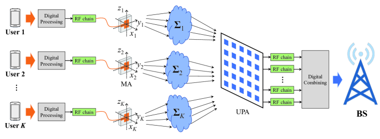
Figure 1: Illustration of the uplink transmission between $K$ single-MA users and the BS equipped with a UPA of size $N=N_{1}\times N_{2}$.

As shown in Fig. 1, the BS is equipped with a uniform planar array (UPA) of size $N=N_{1}\times N_{2}$ to serve $K$ single-MA users, where $N_{1}$ and $N_{2}$ denote the number of antennas along horizontal and vertical directions, respectively. We assume that the number of users does not exceed that of antennas at the BS, i.e., $K\leq N$, and thus the space-division multiple access (SDMA) can be used. For each user $k$, the MA is connected to the RF chain via a flexible cable such that it can be moved in a local region $\mathcal{C}_{k}$. A 3D local coordinate system is established to describe the position of MA for user $k$, which is denoted as $\mathbf{u}_{k}=[x_{k},y_{k},z_{k}]^{\mathrm{T}}\in\mathcal{C}_{k}$, $1\leq k\leq K$. Without loss of generality, we assume that the local region for moving the antenna is a cuboid, i.e., $\mathcal{C}_{k}=\left[x_{k}^{\min},x_{k}^{\max}\right]\times\left[y_{k}^{\min},y_{k}^{\max}\right]\times\left[z_{k}^{\min},z_{k}^{\max}\right]$, $1\leq k\leq K$. Besides, the local coordinate of the $n$-th FPA at the BS is denoted as $\mathbf{v}_{n}=[X_{n},Y_{n},Z_{n}]$, $1\leq n\leq N$.

Let $\mathbf{h}_{k}(\mathbf{u}_{k})\in\mathbb{C}^{N\times 1}$ denote the channel vector between the BS and user $k$, which is determined by the propagation environment and the position of the MA, $\mathbf{u}_{k}$. We consider the uplink transmission from the users to BS, where the received signals via the MAC can be expressed as

$$\mathbf{y}=\mathbf{W}^{\mathrm{H}}\mathbf{H}(\tilde{\mathbf{u}})\mathbf{P}^{1/2}\mathbf{s}+\mathbf{W}^{\mathrm{H}}\mathbf{n},$$ (1)

where $\mathbf{W}=\left[\mathbf{w}_{1},\mathbf{w}_{2},\cdots,\mathbf{w}_{K}\right]\in\mathbb{C}^{N\times K}$ is the receive combining matrix at the BS, and $\mathbf{w}_{k}$ is the combining vector for user $k$, $1\leq k\leq K$. $\mathbf{H}(\tilde{\mathbf{u}})=\left[\mathbf{h}_{1}(\mathbf{u}_{1}),\mathbf{h}_{2}(\mathbf{u}_{2}),\cdots,\mathbf{h}_{K}(\mathbf{u}_{K})\right]\in\mathbb{C}^{N\times K}$ denotes the MAC matrix from all $K$ users to the antenna array of the BS, where $\tilde{\mathbf{u}}=\left[\mathbf{u}_{1}^{\mathrm{T}},\mathbf{u}_{2}^{\mathrm{T}},\cdots,\mathbf{u}_{K}^{\mathrm{T}}\right]^{\mathrm{T}}$ is the MA positioning vector for the $K$ users. $\mathbf{s}=\left[s_{1},s_{2},\cdots,s_{K}\right]^{\mathrm{T}}\in\mathbb{C}^{K\times 1}$ represents the transmitted signals of the users with normalized power, i.e., $\mathbb{E}(\mathbf{s}^{\mathrm{H}}\mathbf{s})=\mathbf{I}_{K}$. $\mathbf{P}^{1/2}=\operatorname{diag}\left\{\sqrt{p}_{1},\sqrt{p}_{2},\cdots,\sqrt{p}_{K}\right\}$ denotes the power scaling matrix with the transmit power of user $k$ given by $p_{k}$, $1\leq k\leq K$. $\mathbf{n}=\left[n_{1},n_{2},\cdots,n_{N}\right]^{\mathrm{T}}\sim\mathcal{CN}(\mathbf{0},\sigma^{2}\mathbf{I}_{N})$ is the additive white Gaussian noise (AWGN) at the BS with $\sigma^{2}$ being the average noise power.

II-A Channel Model

In this paper, we consider narrow-band channels with slow fading and focus on one quasi-static fading block. As we have mentioned, the channel vector between each user and the BS is determined by the propagation environment and the position of MA. For simplicity, we assume that the far-field condition is satisfied between the BS and users, where the sizes of moving regions ($\mathcal{C}_{k}$) for the users and the UPA of the BS are much smaller than the signal propagation distance. Under this assumption, the plane-wave model can be used to form the field response from the MA region of each user to the UPA of the BS. In particular, the angle of departure (AoD), the angle of arrival (AoA), and the amplitude of the complex coefficient for each channel path between the BS and each user do not change for different positions of the MA in its corresponding region, while only the phase of the channel path varies with the MA position [9].

Let $L_{k}^{\mathrm{t}}$ and $L_{k}^{\mathrm{r}}$, $1\leq k\leq K$, denote the total number of transmit and receive channel paths from user $k$ to the BS, respectively. The elevation and azimuth AoDs for the $j$-th transmit path between user $k$ and the BS are denoted as $\theta_{k,j}^{\mathrm{t}}$ and $\phi_{k,j}^{\mathrm{t}}$, $1\leq j\leq L_{k}^{\mathrm{t}}$, respectively. The elevation and azimuth AoAs for the $i$-th receive path between user $k$ and the BS are denoted as $\theta_{k,i}^{\mathrm{r}}$ and $\phi_{k,i}^{\mathrm{r}}$, $1\leq i\leq L_{k}^{\mathrm{r}}$, respectively. For convenience, we define the virtual AoDs and AoAs as

$$\vartheta_{k,j}^{\mathrm{t}}=\cos\theta_{k,j}^{\mathrm{t}}\cos\phi_{k,j}^{\mathrm{t}},~{}\varphi_{k,j}^{\mathrm{t}}=\cos\theta_{k,j}^{\mathrm{t}}\sin\phi_{k,j}^{\mathrm{t}},~{}\omega_{k,j}^{\mathrm{t}}=\sin\theta_{k,j}^{\mathrm{t}},~{}1\leq k\leq K,~{}1\leq j\leq L_{k}^{\mathrm{t}},$$ (2a)

$$\vartheta_{k,i}^{\mathrm{r}}=\cos\theta_{k,i}^{\mathrm{r}}\cos\phi_{k,i}^{\mathrm{r}},~{}\varphi_{k,i}^{\mathrm{r}}=\cos\theta_{k,i}^{\mathrm{r}}\sin\phi_{k,i}^{\mathrm{r}},~{}\omega_{k,i}^{\mathrm{r}}=\sin\theta_{k,i}^{\mathrm{r}},~{}1\leq k\leq K,~{}1\leq i\leq L_{k}^{\mathrm{r}}.$$ (2b)

Denoting $\lambda$ as the carrier wavelength, the transmit and receive field-response vectors (FRVs) for the channel between user $k$ and the BS are obtained as [9, 10]

$$\mathbf{g}_{k}(\mathbf{u}_{k})=\left[\mathrm{e}^{\mathrm{j}\frac{2\pi}{\lambda}\rho_{k,1}^{\mathrm{t}}(\mathbf{u}_{k})},\mathrm{e}^{\mathrm{j}\frac{2\pi}{\lambda}\rho_{k,2}^{\mathrm{t}}(\mathbf{u}_{k})},\cdots,\mathrm{e}^{\mathrm{j}\frac{2\pi}{\lambda}\rho_{k,L_{k}^{\mathrm{t}}}^{\mathrm{t}}(\mathbf{u}_{k})}\right]^{\mathrm{T}},~{}1\leq k\leq K,$$ (3a)

$$\mathbf{f}_{k}(\mathbf{v}_{n})=\left[\mathrm{e}^{\mathrm{j}\frac{2\pi}{\lambda}\rho_{k,1}^{\mathrm{r}}(\mathbf{v}_{n})},\mathrm{e}^{\mathrm{j}\frac{2\pi}{\lambda}\rho_{k,2}^{\mathrm{r}}(\mathbf{v}_{n})},\cdots,\mathrm{e}^{\mathrm{j}\frac{2\pi}{\lambda}\rho_{k,L_{k}^{\mathrm{r}}}^{\mathrm{r}}(\mathbf{v}_{n})}\right]^{\mathrm{T}},~{}1\leq k\leq K,~{}1\leq n\leq N,$$ (3b)

where $\rho_{k,j}^{\mathrm{t}}(\mathbf{u}_{k})=x_{k}\vartheta_{k,j}^{\mathrm{t}}+y_{k}\varphi_{k,j}^{\mathrm{t}}+z_{k}\omega_{k,j}^{\mathrm{t}}$, $1\leq j\leq L_{k}^{\mathrm{t}}$, represents the difference of the signal propagation distance for the $j$-th transmit channel path between MA position $\mathbf{u}_{k}$ and the origin (i.e., $O_{k}$) of the local coordinate system at user $k$. It indicates that the phase difference of the coefficient of the $j$-th transmit channel path for user $k$ between MA locations $\mathbf{u}_{k}$ and $O_{k}$ is given by $\frac{2\pi}{\lambda}\rho_{k,j}^{\mathrm{t}}(\mathbf{u}_{k})$. Thus, the transmit FRV, $\mathbf{g}_{k}(\mathbf{u}_{k})$, characterizes the phase differences in all $L_{k}^{\mathrm{t}}$ transmit paths from user $k$ to the BS. Similarly, the receive FRV, $\mathbf{f}_{k}(\mathbf{v}_{n})$, accounts for the phase differences in all $L_{k}^{\mathrm{r}}$ receive paths from user $k$ to the BS, where $\rho_{k,i}^{\mathrm{r}}(\mathbf{v}_{n})=X_{n}\vartheta_{k,i}^{\mathrm{r}}+Y_{n}\varphi_{k,i}^{\mathrm{r}}+Z_{n}\omega_{k,i}^{\mathrm{r}}$, $1\leq i\leq L_{k}^{\mathrm{r}}$, represents the difference of the signal propagation distance for the $i$-th receive channel path between BS-antenna position $\mathbf{v}_{n}$ and the origin (i.e., $O_{0}$) of the local coordinate system at the BS.

Then, we define the path-response matrix (PRM), $\mathbf{\Sigma}_{k}\in\mathbb{C}^{L_{k}^{\mathrm{r}}\times L_{k}^{\mathrm{t}}}$, to represent the response between all the transmit and receive channel paths from $O_{k}$ to $O_{0}$, $1\leq k\leq K$. Specifically, the entry in the $i$-th row and $j$-th column of $\mathbf{\Sigma}_{k}$ is the response coefficient between the $j$-th transmit path and the $i$-th receive path for user $k$. As a result, the channel vector between user $k$ and the BS can be expressed as [9, 10]

$$\mathbf{h}_{k}(\mathbf{u}_{k})=\mathbf{F}_{k}^{\mathrm{H}}\mathbf{\Sigma}_{k}\mathbf{g}_{k}(\mathbf{u}_{k}),$$ (4)

where $\mathbf{F}_{k}=\left[\mathbf{f}_{k}(\mathbf{v}_{1}),\mathbf{f}_{k}(\mathbf{v}_{2}),\cdots,\mathbf{f}_{k}(\mathbf{v}_{N})\right]\in\mathbb{C}^{L_{k}^{\mathrm{r}}\times N}$ is the field-response matrix (FRM) at the BS, which is a constant matrix because the antennas of the BS have fixed positions. As can be observed from (4), the positioning optimization of the MA for each user can change its FRV, which yields a varying linear combination of the columns in matrix $\mathbf{F}_{k}^{\mathrm{H}}\mathbf{\Sigma}_{k}$. Thus, the channel vector between each user and the BS can be significantly changed by moving the antenna of the user in a local region.

II-B Problem Formulation

For the uplink transmission employing linear combining at the BS, the receive SINR of the signal from user $k$ is given by

$$\gamma_{k}=\frac{\left|\mathbf{w}_{k}^{\mathrm{H}}\mathbf{h}_{k}(\mathbf{u}_{k})\right|^{2}p_{k}}{\sum\limits_{q=1,q\neq k}^{K}\left|\mathbf{w}_{k}^{\mathrm{H}}\mathbf{h}_{q}(\mathbf{u}_{q})\right|^{2}p_{q}+\left\|\mathbf{w}_{k}\right\|_{2}^{2}\sigma^{2}},~{}1\leq k\leq K,$$ (5)

and thus the achievable rate for user $k$ is obtained as $R_{k}=\log_{2}\left(1+\gamma_{k}\right)$.

In this paper, we aim at minimizing the total transmit power of multiple users by jointly optimizing the position of MA for each user, the transmit power of each user, and the receive combining matrix of the BS, subject to a minimum-achievable-rate requirement for each user. Let $\mathbf{p}=[p_{1},p_{2},\cdots,p_{K}]^{\mathrm{T}}$ denote the vector of transmit power of the users. Accordingly, the optimization problem can be formulated as

$$\mathop{\min}\limits_{\tilde{\mathbf{u}},\mathbf{p},\mathbf{W}}~{}~{}~{} \sum\limits_{k=1}^{K}p_{k}$$ (6a)

$$\mathrm{s.t.}~{}~{}~{}~{} \log_{2}\left(1+\gamma_{k}\right)\geq r_{k},~{}1\leq k\leq K,$$ (6b)

$$\mathbf{u}_{k}\in\mathcal{C}_{k},~{}1\leq k\leq K,$$ (6c)

$$p_{k}\geq 0,~{}1\leq k\leq K,$$ (6d)

where constraint (6b) indicates that the achievable rate for user $k$ should be no smaller than its minimum requirement $r_{k}$. Constraint (6c) confines that the MA of user $k$ is located in its moving region, $\mathcal{C}_{k}$. Constraint (6d) guarantees that the transmit power of each user is non-negative. Problem (6) is difficult to solve because the channel vectors and achievable rates of the users are highly non-convex w.r.t. the positions of MAs. Besides, the coupling between these high-dimensional matrix/vector variables makes this problem more intractable. Problem (6) cannot be optimally solved with existing optimization tools in polynomial time. Thus, we develop suboptimal solutions for (6) in the next section.

III Proposed Solution

Due to the coupling between the positions of MAs, the transmit power of users, and the receive combining matrix at the BS, problem (6) cannot be optimally solved efficiently. In general, the alternating optimization among the three matrix/vector variables may lead to a (undesired) local optimum. For example, given the optimal receive combining matrix at the BS designed based on the channel vectors between the BS and users, the optimized positions of MAs cannot be significantly changed compared to those in the last iteration. This is because the channel vectors of other MA positions do not match the receive combining matrix and are highly likely to decrease the effective channel gains of the target signals as well as increase the interference among multiple users. To address this issue, we propose to leverage the ZF and MMSE combining methods for expressing the receive combining matrix as a function of the MA positioning vector, and then optimize the positions of MAs for minimizing the total transmit power of multiple users. The two solutions based on ZF and MMSE combining are presented in the following, respectively.

III-A ZF-Based Solution

For any given positions of MAs, $\tilde{\mathbf{u}}$, the channel vectors between the BS and users are fixed. Thus, the ZF combining matrix can be expressed as a function of the MA positioning vector [26], i.e.,

$$\mathbf{W}_{\mathrm{ZF}}(\tilde{\mathbf{u}})=\left(\mathbf{H}(\tilde{\mathbf{u}})^{\mathrm{H}}\right)^{\dagger}=\mathbf{H}(\tilde{\mathbf{u}})\left(\mathbf{H}(\tilde{\mathbf{u}})^{\mathrm{H}}\mathbf{H}(\tilde{\mathbf{u}})\right)^{-1}\triangleq\left[\bar{\mathbf{w}}_{1},\bar{\mathbf{w}}_{2},\cdots,\bar{\mathbf{w}}_{K}\right].$$ (7)

Substituting (7) into (5), the receive SINR of the signal from user $k$ can be rewritten as

$$\bar{\gamma}_{k}=\frac{p_{k}}{\left\|\bar{\mathbf{w}}_{k}\right\|_{2}^{2}\sigma^{2}}=\frac{p_{k}}{\left\|\mathbf{H}(\tilde{\mathbf{u}})\left[\left(\mathbf{H}(\tilde{\mathbf{u}})^{\mathrm{H}}\mathbf{H}(\tilde{\mathbf{u}})\right)^{-1}\right]_{:,k}\right\|_{2}^{2}\sigma^{2}},~{}1\leq k\leq K.$$ (8)

Furthermore, we substitute (8) into (6b) and obtain the minimum transmit power of user $k$ for satisfying the achievable-rate requirement as

$$\log_{2}\left(1+\bar{\gamma}_{k}\right)\geq r_{k}\Rightarrow\frac{p_{k}}{\left\|\mathbf{H}(\tilde{\mathbf{u}})\left[\left(\mathbf{H}(\tilde{\mathbf{u}})^{\mathrm{H}}\mathbf{H}(\tilde{\mathbf{u}})\right)^{-1}\right]_{:,k}\right\|_{2}^{2}\sigma^{2}}\geq 2^{r_{k}}-1$$ (9)

$$\Rightarrow p_{k}\geq\left\|\mathbf{H}(\tilde{\mathbf{u}})\left[\left(\mathbf{H}(\tilde{\mathbf{u}})^{\mathrm{H}}\mathbf{H}(\tilde{\mathbf{u}})\right)^{-1}\right]_{:,k}\right\|_{2}^{2}\eta_{k}\sigma^{2}\triangleq\bar{p}_{k},~{}1\leq k\leq K,$$

where $\eta_{k}=2^{r_{k}}-1$ represents the minimum-SINR requirement for user $k$. Note that the transmit power shown in (9) is always non-negative, and thus constraint (6d) is satisfied. As a result, the optimal solution for the total transmit power of users for satisfying the minimum-achievable-rate constraint can be expressed as

$$\sum\limits_{k=1}^{K}\bar{p}_{k} =\sum\limits_{k=1}^{K}\left\|\mathbf{H}(\tilde{\mathbf{u}})\left[\left(\mathbf{H}(\tilde{\mathbf{u}})^{\mathrm{H}}\mathbf{H}(\tilde{\mathbf{u}})\right)^{-1}\right]_{:,k}\right\|_{2}^{2}\eta_{k}\sigma^{2}=\left\|\mathbf{H}(\tilde{\mathbf{u}})\left(\mathbf{H}(\tilde{\mathbf{u}})^{\mathrm{H}}\mathbf{H}(\tilde{\mathbf{u}})\right)^{-1}\mathbf{\Omega}^{1/2}\right\|_{\mathrm{F}}^{2}$$ (10)

$$=\operatorname{tr}\left\{\left(\mathbf{H}(\tilde{\mathbf{u}})^{\mathrm{H}}\mathbf{H}(\tilde{\mathbf{u}})\right)^{-1}\mathbf{\Omega}\right\}=\operatorname{tr}\left\{\left(\mathbf{\Omega}^{-1}\mathbf{H}(\tilde{\mathbf{u}})^{\mathrm{H}}\mathbf{H}(\tilde{\mathbf{u}})\right)^{-1}\right\}$$

$$=\sum_{k=1}^{K}\frac{1}{\lambda_{k}\left\{\mathbf{\Omega}^{-1}\mathbf{H}(\tilde{\mathbf{u}})^{\mathrm{H}}\mathbf{H}(\tilde{\mathbf{u}})\right\}}\triangleq g(\tilde{\mathbf{u}}),$$

where $\mathbf{\Omega}=\operatorname{diag}\left\{\eta_{1}\sigma^{2},\eta_{2}\sigma^{2},\cdots,\eta_{K}\sigma^{2}\right\}$ is a diagonal matrix with constant elements.
$\lambda_{k}\left\{\mathbf{\Omega}^{-1}\mathbf{H}(\tilde{\mathbf{u}})^{\mathrm{H}}\mathbf{H}(\tilde{\mathbf{u}})\right\}$ denotes the $k$-th eigenvalue of matrix $\mathbf{\Omega}^{-1}\mathbf{H}(\tilde{\mathbf{u}})^{\mathrm{H}}\mathbf{H}(\tilde{\mathbf{u}})$. Then, problem (6) can be transformed into

$$\mathop{\min}\limits_{\tilde{\mathbf{u}}}~{}~{}~{} g(\tilde{\mathbf{u}})$$ (11a)

$$\mathrm{s.t.}~{}~{}~{}~{} \mathbf{u}_{k}\in\mathcal{C}_{k},~{}1\leq k\leq K.$$ (11b)

Since $g(\tilde{\mathbf{u}})$ is highly non-convex w.r.t. $\tilde{\mathbf{u}}$, it is challenging to obtain the globally optimal solution for problem (11). Next, we employ the gradient descent method to obtain a suboptimal solution. Specifically, the initial MA positioning vector is set as $\tilde{\mathbf{u}}^{(0)}=\mathbf{0}_{3K}$, which means that the MA of each user is initially placed at the origin of its local coordinate system. Let $\tilde{\mathbf{u}}^{(t-1)}$ denote the MA positioning vector obtained in the $(t-1)$-th iteration. The gradient of function $g\left(\tilde{\mathbf{u}}\right)$ at location $\tilde{\mathbf{u}}^{(t-1)}$ can be calculated according to the definition, i.e.,

$$\left[\nabla_{\tilde{\mathbf{u}}}g\left(\tilde{\mathbf{u}}^{(t-1)}\right)\right]_{i}=\frac{\partial g\left(\tilde{\mathbf{u}}\right)}{\partial\left[\tilde{\mathbf{u}}\right]_{i}}{\bigg{|}}_{\tilde{\mathbf{u}}=\tilde{\mathbf{u}}^{(t-1)}}=\lim\limits_{\delta\rightarrow 0}\frac{g\left(\tilde{\mathbf{u}}^{(t-1)}+\delta\mathbf{e}_{3K}^{i}\right)-g\left(\tilde{\mathbf{u}}^{(t-1)}\right)}{\delta},~{}1\leq i\leq 3K,$$ (12)

where $\mathbf{e}_{3K}^{i}$ is a $3K$-dimensional vector with a one as the $i$-th element and zeros elsewhere. Then, the MA positioning vector in the $t$-th iteration is updated by moving along the gradient direction [27], i.e.,

$$\tilde{\mathbf{u}}^{(t)}=\mathcal{B}\left\{\tilde{\mathbf{u}}^{(t-1)}-\bar{\tau}^{(t)}\nabla_{\tilde{\mathbf{u}}}g\left(\tilde{\mathbf{u}}^{(t-1)}\right)\right\},$$ (13)

where $\bar{\tau}^{(t)}$ is the step size for gradient descent in the $t$-th iteration. $\mathcal{B}\left\{\tilde{\mathbf{u}}\right\}$ is a function which projects each element in $\tilde{\mathbf{u}}$ to the nearest boundary of its feasible region if this element exceeds the feasible region, i.e.,

$$\left[\mathcal{B}\left\{\tilde{\mathbf{u}}\right\}\right]_{i}=\left\{\begin{aligned} &\left[\tilde{\mathbf{u}}\right]_{i}^{\min},~{}\text{if }\left[\tilde{\mathbf{u}}\right]_{i}<\left[\tilde{\mathbf{u}}\right]_{i}^{\min},\\ &\left[\tilde{\mathbf{u}}\right]_{i},~{}~{}~{}~{}\text{if }\left[\tilde{\mathbf{u}}\right]_{i}^{\min}\leq\left[\tilde{\mathbf{u}}\right]_{i}\leq\left[\tilde{\mathbf{u}}\right]_{i}^{\max},\\ &\left[\tilde{\mathbf{u}}\right]_{i}^{\max},~{}\text{if }\left[\tilde{\mathbf{u}}\right]_{i}>\left[\tilde{\mathbf{u}}\right]_{i}^{\max},\end{aligned}\right.$$ (14)

where $\left[\tilde{\mathbf{u}}\right]_{i}^{\min}$ and $\left[\tilde{\mathbf{u}}\right]_{i}^{\max}$ denote the lower-bound and upper-bound on the feasible region of the $i$-th element of $\tilde{\mathbf{u}}$, respectively. According to the definition $\tilde{\mathbf{u}}=\left[\mathbf{u}_{1}^{\mathrm{T}},\mathbf{u}_{2}^{\mathrm{T}},\cdots,\mathbf{u}_{K}^{\mathrm{T}}\right]^{\mathrm{T}}$, the $i$-th element of $\tilde{\mathbf{u}}$ corresponds to the $q_{i}$-th element of $\mathbf{u}_{k_{i}}$, with $k_{i}=\lfloor i/3\rfloor+1$ and $q_{i}=i-3(k_{i}-1)$. The utilization of projection function $\mathcal{B}\left\{\tilde{\mathbf{u}}\right\}$ is to ensure that the solution for MA positioning is always located in the feasible region during the iterations. As we know, the step size significantly impacts the performance of the gradient descent algorithm. In this paper, we employ the backtracking line search to obtain an appropriate step size [28]. Specifically, for each iteration, we start with a large positive step size, $\bar{\tau}^{(t)}=\bar{\tau}$, and repeatedly shrink it by a factor $\bar{\kappa}\in(0,1)$, i.e., $\bar{\tau}^{(t)}\leftarrow\bar{\kappa}\bar{\tau}^{(t)}$, until the Armijo–Goldstein condition is satisfied, i.e.,

$$g(\tilde{\mathbf{u}}^{(t)})\leq g(\tilde{\mathbf{u}}^{(t-1)})-\bar{\xi}\bar{\tau}^{(t)}\left\|\nabla_{\tilde{\mathbf{u}}}g\left(\tilde{\mathbf{u}}^{(t-1)}\right)\right\|_{2}^{2},$$ (15)

where $\bar{\xi}\in(0,1)$ is a given control parameter to evaluate whether the current step size achieves an adequate decrease in the objective function. The overall algorithm terminates until the decrement on the objective value in (6a) is below a small positive value, $\bar{\epsilon}$.

0:   $N$, $K$, $\sigma^{2}$, $\lambda$, $\{\mathcal{C}_{k}\}$ $\{r_{k}\}$, $\{\mathbf{\Sigma}_{k}\}$, $\{\mathbf{F}_{k}\}$, $\{\theta_{k,j}^{\mathrm{t}}\}$, $\{\phi_{k,j}^{\mathrm{t}}\}$, $\bar{\tau}$, $\bar{\xi}$, $\bar{\kappa}$, $\bar{\epsilon}$, $\bar{T}_{\max}$. 0:   $\tilde{\mathbf{u}}_{\mathrm{ZF}}$, $\mathbf{W}_{\mathrm{ZF}}$, $\mathbf{p}_{\mathrm{ZF}}$. 1:  Initialize $\tilde{\mathbf{u}}^{(0)}=\mathbf{0}_{3K}$. 2:  Obtain $g(\tilde{\mathbf{u}})$ according to (10). 3:  for $t=1:1:\bar{T}_{\max}$ do 4:     Calculate the gradient value $\nabla_{\tilde{\mathbf{u}}}g\left(\tilde{\mathbf{u}}^{(t-1)}\right)$ according to (12). 5:     Initialize the step size $\bar{\tau}^{(t)}=\bar{\tau}$. 6:     Update MA positioning vector $\tilde{\mathbf{u}}^{(t)}$ according to (13). 7:     while $g(\tilde{\mathbf{u}}^{(t)})>g(\tilde{\mathbf{u}}^{(t-1)})-\bar{\xi}\bar{\tau}^{(t)}\left\|\nabla_{\tilde{\mathbf{u}}}g\left(\tilde{\mathbf{u}}^{(t-1)}\right)\right\|_{2}^{2}$ do 8:        Shrink the step size $\bar{\tau}^{(t)}\leftarrow\bar{\kappa}\bar{\tau}^{(t)}$. 9:        Update MA positioning vector $\tilde{\mathbf{u}}^{(t)}$ according to (13). 10:     end while 11:     if $\left|g(\tilde{\mathbf{u}}^{(t)})-g(\tilde{\mathbf{u}}^{(t-1)})\right|<\bar{\epsilon}$ then 12:        Break. 13:     end if 14:  end for 15:  Set the MA positioning vector as $\tilde{\mathbf{u}}_{\mathrm{ZF}}=\tilde{\mathbf{u}}^{(t)}$. 16:  Calculate the ZF combining matrix $\mathbf{W}_{\mathrm{ZF}}$ according to (7). 17:  Calculate the transmit power $\mathbf{p}_{\mathrm{ZF}}$ according to (9). 18:  return  $\tilde{\mathbf{u}}_{\mathrm{ZF}}$, $\mathbf{W}_{\mathrm{ZF}}$, $\mathbf{p}_{\mathrm{ZF}}$.

Algorithm 1 The ZF-based solution for solving problem (6).

The ZF-based solution for solving problem (6) is summarized in Algorithm 1, where $\bar{T}_{\max}$ denotes the maximum number of iterations. In lines 3-14, the MA positioning vector is iteratively updated by using the gradient descent method, where the step size in each iteration is obtained by backtracking line search in lines 7-10. The convergence of Algorithm 1 is analyzed as follows. On one hand, due to the fact of $\bar{\tau}^{(t)}>0$, $\bar{\xi}>0$, and $\left\|\nabla_{\tilde{\mathbf{u}}}g\left(\tilde{\mathbf{u}}^{(t-1)}\right)\right\|_{2}^{2}\geq 0$, we always have $g(\tilde{\mathbf{u}}^{(t)})\leq g(\tilde{\mathbf{u}}^{(t-1)})$ during the iterations. On the other hand, for the case of $\left\|\nabla_{\tilde{\mathbf{u}}}g\left(\tilde{\mathbf{u}}^{(t-1)}\right)\right\|_{2}^{2}>0$, according to the definition of gradient, we can always find a sufficiently small positive $\bar{\tau}^{(t)}$ satisfying $g(\tilde{\mathbf{u}}^{(t)})<g(\tilde{\mathbf{u}}^{(t-1)})$, unless all elements of $\tilde{\mathbf{u}}^{(t-1)}$ with nonzero partial derivatives are located on the boundary of the feasible region as well as the corresponding gradient direction is towards the outside of the feasible region. Thus, Algorithm 1 terminates at a solution with the gradient equal to zero or a solution located on the boundary of the feasible region defined by (11b), which yields a local optimum for problem (6). To improve the capability of global search, the initial step size, $\bar{\tau}$, should be set sufficiently large such that the solution can get rid of the local optimum. In Algorithm 1, the computational complexity for calculating the gradient value in line 4 is $\mathcal{O}(K^{3}N)$. Denoting the maximum number of iterations for backtracking line search in lines 7-10 as $\bar{I}_{\max}$, the corresponding computational complexity is given by $\mathcal{O}(\bar{I}_{\max}K^{2}N)$. As a result, the maximum computational complexity of Algorithm 1 for solving problem (6) is $\mathcal{O}\left(\bar{T}_{\max}(K^{3}N+\bar{I}_{\max}K^{2}N)\right)$.

III-B MMSE-Based Solution

For any given MA positioning vector (i.e., $\tilde{\mathbf{u}}$) and transmit power of the users (i.e., $\mathbf{p}$), the optimal linear combining matrix of the BS for maximizing the achievable rate region is given by the MMSE receiver [26], i.e.,

$$\mathbf{W}_{\mathrm{MMSE}}(\tilde{\mathbf{u}},\mathbf{P})=\left(\mathbf{H}(\tilde{\mathbf{u}})\mathbf{P}\mathbf{H}(\tilde{\mathbf{u}})^{\mathrm{H}}+\sigma^{2}\mathbf{I}_{N}\right)^{-1}\mathbf{H}(\tilde{\mathbf{u}})\triangleq\left[\hat{\mathbf{w}}_{1},\hat{\mathbf{w}}_{2},\cdots,\hat{\mathbf{w}}_{K}\right],$$ (16)

with $\mathbf{P}=\operatorname{diag}\{\mathbf{p}\}$ and $\hat{\mathbf{w}}_{k}=\left(\mathbf{H}(\tilde{\mathbf{u}})\mathbf{P}\mathbf{H}(\tilde{\mathbf{u}})^{\mathrm{H}}+\sigma^{2}\mathbf{I}_{N}\right)^{-1}\mathbf{h}_{k}(\mathbf{u}_{k})$, $1\leq k\leq K$. Substituting (16) into (5), the receive SINR of the signal from user $k$ can be rewritten as

$$\hat{\gamma}_{k} =\frac{\left|\hat{\mathbf{w}}_{k}^{\mathrm{H}}\mathbf{h}_{k}(\mathbf{u}_{k})\right|^{2}p_{k}}{\sum\limits_{q=1,q\neq k}^{K}\left|\hat{\mathbf{w}}_{k}^{\mathrm{H}}\mathbf{h}_{q}(\mathbf{u}_{q})\right|^{2}p_{q}+\left\|\hat{\mathbf{w}}_{k}\right\|_{2}^{2}\sigma^{2}}\triangleq\frac{A_{k,k}p_{k}}{\sum\limits_{q=1,q\neq k}^{K}A_{k,q}p_{q}+b_{k}},~{}1\leq k\leq K,$$ (17)

where $A_{k,q}\triangleq\left|\hat{\mathbf{w}}_{k}^{\mathrm{H}}\mathbf{h}_{q}(\mathbf{u}_{q})\right|^{2}=\left|\mathbf{h}_{k}(\mathbf{u}_{k})^{\mathrm{H}}\left(\mathbf{H}(\tilde{\mathbf{u}})\mathbf{P}\mathbf{H}(\tilde{\mathbf{u}})^{\mathrm{H}}+\sigma^{2}\mathbf{I}_{N}\right)^{-1}\mathbf{h}_{q}(\mathbf{u}_{q})\right|^{2}$ and $b_{k}\triangleq\left\|\hat{\mathbf{w}}_{k}\right\|_{2}^{2}\sigma^{2}=\left\|\left(\mathbf{H}(\tilde{\mathbf{u}})\mathbf{P}\mathbf{H}(\tilde{\mathbf{u}})^{\mathrm{H}}+\sigma^{2}\mathbf{I}_{N}\right)^{-1}\mathbf{h}_{k}(\mathbf{u}_{k})\right\|_{2}^{2}\sigma^{2}$, $1\leq k\leq K$ and $1\leq q\leq K$.

Let $\mathbf{A}\in\mathbb{R}^{K\times K}$ denote a matrix with the entry in the $k$-th row and $q$-th column given by $A_{k,q}$, and $\mathbf{b}\in\mathbb{R}^{K\times 1}$ denote a vector with the $k$-th entry given by $b_{k}$. It is easy to verify that to minimize the total transmit power, the SINR of each user should be exactly equal to its minimum requirement, i.e., $\hat{\gamma}_{k}=\eta_{k}$ [23], which can be equivalently expressed as $A_{k,k}/\eta_{k}\times p_{k}=\sum_{q=1,q\neq k}^{K}A_{k,q}p_{q}+b_{k}$, $1\leq k\leq K$. The matrix form of these equations w.r.t. $\mathbf{p}$ is given by

$$\left(\mathbf{D}-\mathbf{\Psi}\right)\mathbf{p}=\mathbf{b},$$ (18)

with $\mathbf{D}=\operatorname{diag}\{A_{1,1}/\eta_{1},A_{2,2}/\eta_{2},\cdots,A_{K,K}/\eta_{K}\}$, $\left[\mathbf{\Psi}\right]_{k,q}=A_{k,q}$ for $1\leq k\neq q\leq K$ and $\left[\mathbf{\Psi}\right]_{k,k}=0$ for $1\leq k\leq K$. Thus, the optimal solution for the transmit power is obtained as

$$\hat{\mathbf{p}}=\left(\mathbf{D}-\mathbf{\Psi}\right)^{-1}\mathbf{b}.$$ (19)

The total transmit power of users for satisfying the minimum-achievable-rate constraint can be expressed as

$$\sum\limits_{k=1}^{K}\hat{p}_{k}=\left\|\left(\mathbf{D}-\mathbf{\Psi}\right)^{-1}\mathbf{b}\right\|_{1}\triangleq f(\tilde{\mathbf{u}},\mathbf{P}).$$ (20)

Note that an implicit constraint should be considered to ensure that the transmit power of each user is non-negative, i.e., $\hat{p}_{k}\geq 0$, $1\leq k\leq K$. It has been shown in [23] that the non-negative power constraint is equivalent to that the spectral radius of matrix $\mathbf{D}\mathbf{\Psi}^{-1}$ is smaller than 1. Then, problem (6) can be transformed into

$$\mathop{\min}\limits_{\tilde{\mathbf{u}},\mathbf{P}}~{}~{}~{} f(\tilde{\mathbf{u}},\mathbf{P})$$ (21a)

$$\mathrm{s.t.}~{}~{}~{}~{} \mathbf{u}_{k}\in\mathcal{C}_{k},~{}1\leq k\leq K,$$ (21b)

$$\rho\left\{\mathbf{D}\mathbf{\Psi}^{-1}\right\}<1,$$ (21c)

where $\rho\left\{\mathbf{D}\mathbf{\Psi}^{-1}\right\}$ represents the spectral radius of matrix $\mathbf{D}\mathbf{\Psi}^{-1}$, which is equal to the maximum of the absolute values of its eigenvalues.

Problem (21) is more challenging to solve compared to (11) due to the following reasons. On one hand, constraint (21c) is non-convex w.r.t. the optimization variables. On the other hand, the MA positioning vector and the transmit power matrix are highly coupled in the objective function of (21a). To tackle this non-convex problem, we propose an iterative algorithm to alternately update $\tilde{\mathbf{u}}$ and $\mathbf{P}$. Specifically, the MA positioning vector is initialized as $\tilde{\mathbf{u}}^{(0)}=\mathbf{0}_{3K}$. Under the given MA positioning, the initial transmit power is $\mathbf{P}^{(0)}$ obtained by alternately optimizing the MMSE combining matrix of the BS according to (16) and the transmit power of users according to (19) until the total transmit power is minimized. Let $\tilde{\mathbf{u}}^{(t-1)}$ and $\mathbf{P}^{(t-1)}$ denote the solution for MA positioning and transmit power in the $(t-1)$-th iteration, respectively. The gradient of function $f(\tilde{\mathbf{u}},\mathbf{P})$ w.r.t. $\tilde{\mathbf{u}}$ at location $(\tilde{\mathbf{u}}^{(t-1)},\mathbf{P}^{(t-1)})$ can be calculated as

$$\left[\nabla_{\tilde{\mathbf{u}}}f\left(\tilde{\mathbf{u}}^{(t-1)},\mathbf{P}^{(t-1)}\right)\right]_{i}=\frac{\partial f\left(\tilde{\mathbf{u}},\mathbf{P}\right)}{\partial\left[\tilde{\mathbf{u}}\right]_{i}}{\bigg{|}}_{\tilde{\mathbf{u}}=\tilde{\mathbf{u}}^{(t-1)},\mathbf{P}=\mathbf{P}^{(t-1)}}$$ (22)

$$= \lim\limits_{\delta\rightarrow 0}\frac{f\left(\tilde{\mathbf{u}}^{(t-1)}+\delta\mathbf{e}_{3K}^{i},\mathbf{P}^{(t-1)}\right)-f\left(\tilde{\mathbf{u}}^{(t-1)},\mathbf{P}^{(t-1)}\right)}{\delta},~{}1\leq i\leq 3K,$$

where $\mathbf{e}_{3K}^{i}$ is a $3K$-dimensional vector with a one as the $i$-th element and zeros elsewhere. Then, the MA positioning vector in the $t$-th iteration is updated according to the gradient descent method [27], i.e.,

$$\tilde{\mathbf{u}}^{(t)}=\mathcal{B}\left\{\tilde{\mathbf{u}}^{(t-1)}-\hat{\tau}^{(t)}\nabla_{\tilde{\mathbf{u}}}f\left(\tilde{\mathbf{u}}^{(t-1)},\mathbf{P}^{(t-1)}\right)\right\},$$ (23)

where $\hat{\tau}^{(t)}$ is the step size for gradient descent in the $t$-th iteration. $\mathcal{B}\left\{\tilde{\mathbf{u}}\right\}$ is the projection function defined in (14), which can ensure that the solution for MA positioning is always located in the feasible region during the iterations. Similarly to Section III-A, the step size is selected by backtracking line search [28]. For each iteration, we start with a large positive step size, $\hat{\tau}^{(t)}=\bar{\tau}$, and repeatedly shrink it by a factor $\hat{\kappa}\in(0,1)$, i.e., $\hat{\tau}^{(t)}\leftarrow\hat{\kappa}\hat{\tau}^{(t)}$, until the Armijo–Goldstein condition and the spectral radius constraint are both satisfied, i.e,

$$f\left(\tilde{\mathbf{u}}^{(t)},\mathbf{P}^{(t-1)}\right)\leq f\left(\tilde{\mathbf{u}}^{(t-1)},\mathbf{P}^{(t-1)}\right)-\hat{\xi}\hat{\tau}^{(t)}\left\|\nabla_{\tilde{\mathbf{u}}}f\left(\tilde{\mathbf{u}}^{(t-1)},\mathbf{P}^{(t-1)}\right)\right\|_{2}^{2},$$ (24a)

$$\rho\left\{\mathbf{D}^{(t)}(\mathbf{\Psi}^{(t)})^{-1}\right\}<1,$$ (24b)

where $\hat{\xi}\in(0,1)$ is a given control parameter to evaluate whether the current step size achieves an adequate decrease in the objective function.

After updating the MA positioning vector, we calculate the values of $\mathbf{D}^{(t)}$, $\mathbf{\Psi}^{(t)}$, $\mathbf{b}^{(t)}$, and $\hat{\mathbf{p}}^{(t)}$ according to (19). The transmit power matrix in the $t$-th iteration is thus updated as

$$\mathbf{P}^{(t)}=\operatorname{diag}\{\hat{\mathbf{p}}^{(t)}\}.$$ (25)

The overall algorithm terminates until the decrement on the objective value in (6a) is below a small positive value, $\bar{\epsilon}$.

0:   $N$, $K$, $\sigma^{2}$, $\lambda$, $\{\mathcal{C}_{k}\}$ $\{r_{k}\}$, $\{\mathbf{\Sigma}_{k}\}$, $\{\mathbf{F}_{k}\}$, $\{\theta_{k,j}^{\mathrm{t}}\}$, $\{\phi_{k,j}^{\mathrm{t}}\}$, $\hat{\tau}$, $\hat{\xi}$, $\hat{\kappa}$, $\hat{\epsilon}$, $\hat{T}_{\max}$. 0:   $\tilde{\mathbf{u}}_{\mathrm{MMSE}}$, $\mathbf{W}_{\mathrm{MMSE}}$, $\mathbf{p}_{\mathrm{MMSE}}$. 1:  Initialize $\tilde{\mathbf{u}}^{(0)}=\mathbf{0}_{3K}$ and $\mathbf{p}$ according to (9). 2:  while The decrement on $\sum_{k=1}^{K}p_{k}$ is larger than $\hat{\epsilon}$ do 3:     Update $\mathbf{P}=\operatorname{diag}\{\mathbf{p}\}$. 4:     Update $\mathbf{W}_{\mathrm{MMSE}}$ according to (16). 5:     Update $\mathbf{p}$ according to (19). 6:  end while 7:  Initialize $\mathbf{P}^{(0)}=\operatorname{diag}\{\mathbf{p}\}$. 8:  Obtain $f(\tilde{\mathbf{u}},\mathbf{P})$ according to (20). 9:  for $t=1:1:\hat{T}_{\max}$ do 10:     Calculate the gradient value $\nabla_{\tilde{\mathbf{u}}}f\left(\tilde{\mathbf{u}}^{(t-1)},\mathbf{P}^{(t-1)}\right)$ according to (22). 11:     Initialize the step size $\hat{\tau}^{(t)}=\hat{\tau}$. 12:     Update MA positioning vector $\tilde{\mathbf{u}}^{(t)}$ according to (23). 13:     Calculate $\mathbf{D}^{(t)}$, $\mathbf{\Psi}^{(t)}$, $\mathbf{b}^{(t)}$, and $\hat{\mathbf{p}}^{(t)}$ according to (19). 14:     while $f\left(\tilde{\mathbf{u}}^{(t)},\mathbf{P}^{(t-1)}\right)>f\left(\tilde{\mathbf{u}}^{(t-1)},\mathbf{P}^{(t-1)}\right)-\hat{\xi}\hat{\tau}^{(t)}\left\|\nabla_{\tilde{\mathbf{u}}}f\left(\tilde{\mathbf{u}}^{(t-1)},\mathbf{P}^{(t-1)}\right)\right\|_{2}^{2}$ or $\rho\left\{\mathbf{D}^{(t)}(\mathbf{\Psi}^{(t)})^{-1}\right\}\geq 1$ do 15:        Shrink the step size $\hat{\tau}^{(t)}\leftarrow\hat{\kappa}\hat{\tau}^{(t)}$. 16:        Update MA positioning vector $\tilde{\mathbf{u}}^{(t)}$ according to (23). 17:        Calculate $\mathbf{D}^{(t)}$, $\mathbf{\Psi}^{(t)}$, $\mathbf{b}^{(t)}$, and $\hat{\mathbf{p}}^{(t)}$ according to (19). 18:     end while 19:     Update $\mathbf{P}^{(t)}$ according to (25). 20:     if $\left|f\left(\tilde{\mathbf{u}}^{(t)},\mathbf{P}^{(t)}\right)-f\left(\tilde{\mathbf{u}}^{(t-1)},\mathbf{P}^{(t-1)}\right)\right|<\bar{\epsilon}$ then 21:        Break. 22:     end if 23:  end for 24:  Set the MA positioning vector as $\tilde{\mathbf{u}}_{\mathrm{MMSE}}=\tilde{\mathbf{u}}^{(t)}$. 25:  Set the transmit power as $\mathbf{p}_{\mathrm{MMSE}}=\hat{\mathbf{p}}^{(t)}$. 26:  Calculate the MMSE combining matrix $\mathbf{W}_{\mathrm{MMSE}}$ according to (16). 27:  return  $\tilde{\mathbf{u}}_{\mathrm{MMSE}}$, $\mathbf{W}_{\mathrm{MMSE}}$, $\mathbf{p}_{\mathrm{MMSE}}$.

Algorithm 2 The MMSE-based solution for solving problem (6).

The MMSE-based solution for solving problem (6) is summarized in Algorithm 2, where $\hat{T}_{\max}$ denotes the maximum number of iterations. In line 1, the MA positioning vector is initialized as $\tilde{\mathbf{u}}^{(0)}=\mathbf{0}_{3K}$. Under the given $\tilde{\mathbf{u}}^{(0)}$, the initial $\mathbf{P}^{(0)}$ is obtained by alternately optimizing the receive combining matrix and the transmit power in lines 2-7. Subsequently, the MA positioning vector and the transmit power matrix are alternately optimized in lines 9-23, where the MMSE combining matrix is written as a function of $\tilde{\mathbf{u}}$ and $\mathbf{P}$ for joint optimization. The convergence of Algorithm 2 is analyzed as follows. For each iteration, the update of the MA positioning vector in lines 14-18 can guarantee that the objective value is non-increasing. This is because $f\left(\tilde{\mathbf{u}},\mathbf{P}^{(t-1)}\right)$ and $\rho\left\{\mathbf{D}\mathbf{\Psi}^{-1}\right\}$ are both continuous functions w.r.t. $\tilde{\mathbf{u}}$. If there exists an element in $\nabla_{\tilde{\mathbf{u}}}f\left(\tilde{\mathbf{u}}^{(t-1)},\mathbf{P}^{(t-1)}\right)$ which is not equal to zero and the corresponding gradient direction is toward the inside of the feasible region, we can always find a sufficiently small positive $\hat{\tau}^{(t)}$ which can guarantee $f\left(\tilde{\mathbf{u}}^{(t)},\mathbf{P}^{(t-1)}\right)<f\left(\tilde{\mathbf{u}}^{(t-1)},\mathbf{P}^{(t-1)}\right)$. Besides, since we have $\rho\left\{\mathbf{D}^{(t-1)}(\mathbf{\Psi}^{(t-1)})^{-1}\right\}<1$, a sufficiently small $\hat{\tau}^{(t)}$ can also guarantee $\rho\left\{\mathbf{D}^{(t)}(\mathbf{\Psi}^{(t)})^{-1}\right\}<1$ due to the continuity of function $\rho\left\{\mathbf{D}\mathbf{\Psi}^{-1}\right\}$. Thus, during the iterations, we can always find a new solution ensuring

$$f\left(\tilde{\mathbf{u}}^{(t)},\mathbf{P}^{(t-1)}\right)\leq f\left(\tilde{\mathbf{u}}^{(t-1)},\mathbf{P}^{(t-1)}\right),$$ (26)

where the equality holds at a point with zero gradient or a point located on the boundary of the feasible region defined by (21b). Moreover, since $\mathbf{P}^{(t)}$ is updated as $\operatorname{diag}\{\hat{\mathbf{p}}^{(t)}\}$ in line 19, which yields an optimal MMSE combining matrix, $\mathbf{W}_{\mathrm{MMSE}}(\tilde{\mathbf{u}}^{(t)},\mathbf{P}^{(t)})$, for maximizing the achievable rate region of the users under the current transmit power $\hat{\mathbf{p}}^{(t)}$ [26]. This indicates that the SINR of each user achieved by $\mathbf{W}_{\mathrm{MMSE}}(\tilde{\mathbf{u}}^{(t)},\mathbf{P}^{(t)})$ and $\hat{\mathbf{p}}^{(t)}$ is no smaller than that achieved by $\mathbf{W}_{\mathrm{MMSE}}(\tilde{\mathbf{u}}^{(t)},\mathbf{P}^{(t-1)})$ and $\hat{\mathbf{p}}^{(t)}$, i.e., $\gamma_{k}\left(\mathbf{W}_{\mathrm{MMSE}}(\tilde{\mathbf{u}}^{(t)},\mathbf{P}^{(t)}),\hat{\mathbf{p}}^{(t)}\right)\geq\gamma_{k}\left(\mathbf{W}_{\mathrm{MMSE}}(\tilde{\mathbf{u}}^{(t)},\mathbf{P}^{(t-1)}),\hat{\mathbf{p}}^{(t)}\right)$, $1\leq k\leq K$. In other words, the updated $\mathbf{P}^{(t)}$ provides additional DoFs for decreasing the total transmit power when solving equations $\hat{\gamma}_{k}=\eta_{k}$, $1\leq k\leq K$. Thus, we have

$$f\left(\tilde{\mathbf{u}}^{(t)},\mathbf{P}^{(t)}\right)\leq f\left(\tilde{\mathbf{u}}^{(t)},\mathbf{P}^{(t-1)}\right).$$ (27)

Combining (26) and (27), we know that Algorithm 2 can achieve a non-increasing sequence of the objective value in (6a) during the iterations. Since the total transmit power is lower-bounded by zero, we can conclude that the convergence of Algorithm 2 for solving problem (6) is guaranteed.

In Algorithm 1, the main computational complexity is caused by the iterations in lines 9-23. Specifically, the calculation of the gradient value in line 10 entails a computational complexity of $\mathcal{O}(KN^{3})$. Denoting the maximum number of iterations for backtracking line search in lines 14-18 as $\hat{I}_{\max}$, the corresponding computational complexity is given by $\mathcal{O}(\hat{I}_{\max}N^{3})$. As a result, the maximum computational complexity of Algorithm 2 for solving problem (6) is $\mathcal{O}\left(\hat{T}_{\max}(KN^{3}+\hat{I}_{\max}N^{3})\right)$.

III-C Alternative Solution for the Single-User Case

In this subsection, we consider a special case where only a single user with MA is served by the BS. As such, the ZF and MMSE combining methods are both degraded into the maximum ratio combining (MRC) because no interference exists. Thus, the optimal MRC vector of the BS is given by

$$\mathbf{w}_{\mathrm{MRC}}(\mathbf{u})=\mathbf{h}(\mathbf{u}),$$ (28)

where $\mathbf{h}(\mathbf{u})\in\mathbb{C}^{N\times 1}$ denotes the channel vector between the BS and the user defined in (4), and $\mathbf{u}=[x,y,z]^{\mathrm{T}}$ is the MA position of the user. The receive SNR of the signal can be obtained as

$$\tilde{\gamma}_{k}=\frac{\left|\mathbf{w}_{\mathrm{MRC}}(\mathbf{u})^{\mathrm{H}}\mathbf{h}(\mathbf{u})\right|^{2}p}{\left\|\mathbf{w}_{\mathrm{MRC}}(\mathbf{u})\right\|_{2}^{2}\sigma^{2}}=\frac{\left\|\mathbf{h}(\mathbf{u})\right\|_{2}^{2}p}{\sigma^{2}},$$ (29)

where $p$ is the transmit power of the user. To satisfy constraint (6b), the minimum transmit power of the user should be given by

$$\tilde{p}=\frac{\eta\sigma^{2}}{\left\|\mathbf{h}(\mathbf{u})\right\|_{2}^{2}},$$ (30)

where $\eta=2^{r}-1$ and $r$ represents the minimum-achievable-rate requirement for the user. To minimize the transmit power of the user, we only need to maximize the gain of the channel vector, i.e.,

$$\mathop{\max}\limits_{\mathbf{u}}~{}~{}~{} \left\|\mathbf{h}(\mathbf{u})\right\|_{2}^{2}$$ (31a)

$$\mathrm{s.t.}~{}~{}~{}~{} \mathbf{u}\in\mathcal{C},$$ (31b)

where $\mathcal{C}$ is the region for moving the antenna of the user. Problem (31) can be solved by using the gradient ascent method similar to the procedures in Sections III-A and III-B. Different from problems (11) and (21), the objective function in (31a) is more tractable and its gradient can be obtained in closed form. The derivation of the gradient for function $\left\|\mathbf{h}(\mathbf{u})\right\|_{2}^{2}$ w.r.t. $\mathbf{u}$ is provided in the Appendix. Then, the gradient ascent method can be applied to problem (31) with the step size in each iteration obtained by backtracking line search [28], which is similar to the procedures in Algorithms 1 and 2.

IV Simulation Results

In this section, we show simulation results to evaluate the performance of the proposed MA-enabled multiple access systems. We first provide the simulation setup and benchmark schemes, and then present the numerical results for verifying the efficacy of the proposed algorithms.

IV-A Simulation Setup and Benchmark Schemes

In the simulation, the users are randomly distributed around the BS with their distance following uniform distribution from 20 to 100 meters (m), i.e., $d_{k}\sim\mathcal{U}[20,100]$, $1\leq k\leq K$. We adopt the channel model in (4), where the numbers of transmit and receive channel paths for each user are the same, i.e., $L_{k}^{\mathrm{t}}=L_{k}^{\mathrm{r}}=L$, $1\leq k\leq K$. For each user, the PRM, $\mathbf{\Sigma}_{k}=\operatorname{diag}\{\sigma_{1},\sigma_{2},\cdots,\sigma_{L}\}$, is a diagonal matrix with each diagonal element following CSCG distribution $\mathcal{CN}(0,c_{k}^{2}/L)$, where $c_{k}=c_{0}d_{k}^{-\alpha}$ is the expected channel gain of user $k$, $c_{0}$ denotes the expected value of the average channel gain at the reference distance of 1 m, and $\alpha$ represents the path-loss exponent. Note that for a fair comparison, the total power of the elements in the PRM is the same for the channels of a user with different numbers of paths, i.e., $\mathbb{E}\{\operatorname{tr}(\mathbf{\Sigma}_{k}^{\mathrm{H}}\mathbf{\Sigma}_{k})\}\equiv c_{k}^{2}$. The elevation and azimuth AoDs of the channel paths for each user are random variables with the joint probability density function (PDF) $f_{\mathrm{AoD}}(\theta_{k}^{\mathrm{t}},\phi_{k}^{\mathrm{t}})=\frac{\cos\theta_{k}^{\mathrm{t}}}{2\pi}$, $\theta_{k}^{\mathrm{t}}\in[-\pi/2,\pi/2]$, $\phi^{\mathrm{t}}\in[-\pi/2,\pi/2]$, which indicates that the AoD has the same probability for all directions in the front half-space of antenna [9]. Due to limited scatters around the BS, the AoAs of channel paths for multiple users are randomly selected from the same set of angles. Specifically, for each channel realization, $S$ pairs of elevation and azimuth AoAs are randomly generated with the joint PDF $f_{\mathrm{AoA}}(\theta^{\mathrm{r}},\phi^{\mathrm{r}})=\frac{\cos\theta^{\mathrm{r}}}{2\pi}$, $\theta^{\mathrm{r}}\in[-\pi/2,\pi/2]$, $\phi^{\mathrm{r}}\in[-\pi/2,\pi/2]$. Then, the $L$ elevation and azimuth AoAs for each user are randomly selected out of the $S$ candidates. The spatial region for moving the antenna at each user is set as a cubical area of size $[-J/2,J/2]\times[-J/2,J/2]\times[-J/2,J/2]$. The minimum-achievable-rate requirements for all $K$ users are set as the same value, i.e., $r_{k}=r$, $1\leq k\leq K$, in bits per second per hertz (bps/Hz). The adopted settings of simulation parameters are provided in Table I, unless specified otherwise. Each point in the simulation figures is the average result over $10^{3}$ user distributions and channel realizations.

TABLE I: Simulation Parameters

Parameter	Description	Value
$N_{1}\times N_{2}$	Antenna array size at the BS	4 $\times$ 4
$K$	Number of users	12
$L$	Number of channel paths for each user	6
$S$	Total number of AoAs at the BS	20
$\lambda$	Carrier wavelength	0.01 m
$c_{0}$	Average channel gain at reference distance	-40 dB
$\alpha$	Exponent of path loss	2.8
$\sigma^{2}$	Noise power	-80 dBm
$J$	Length of the sides of moving region $\mathcal{C}_{k}$	2$\lambda$
$r$	Minimum-achievable-rate requirement for each user	3 bps/Hz
$\bar{T}_{\max}$	Maximum number of iterations in Algorithm 1	200
$\bar{\tau}$	Initial step size for gradient descent in Algorithm 1	10
$\bar{\kappa}$	Scaling factor for shrinking the step size in Algorithm 1	0.5
$\bar{\xi}$	Control parameter for backtracking line search in Algorithm 1	0.6
$\bar{\epsilon}$	Decrement threshold for terminating Algorithm 1	10-6
$\hat{T}_{\max}$	Maximum number of iterations in Algorithm 2	200
$\hat{\tau}$	Initial step size for gradient descent in Algorithm 2	10
$\hat{\kappa}$	Scaling factor for shrinking the step size in Algorithm 2	0.5
$\hat{\xi}$	Control parameter for backtracking line search in Algorithm 2	0.6
$\hat{\epsilon}$	Decrement threshold for terminating Algorithm 2	10-6

In this section, the solutions obtained by Algorithms 1 and 2 are termed as “Proposed MA-ZF” and “Proposed MA-MMSE”, respectively. Two benchmark schemes for antenna positioning are defined as follows. For the FPA scheme, it is assumed that the antenna of each user is fixed at the origin of its local coordinate system, i.e., $\mathbf{u}_{k}^{\circ}=[0,0,0]^{\mathrm{T}}$, $1\leq k\leq K$. For the maximum channel power (MCP) scheme, the MA of each user is deployed at the position which maximizes its channel power, i.e., $\mathbf{u}_{k}^{\star}=\mathop{\arg\max}\limits_{\mathbf{u}_{k}\in\mathcal{C}_{k}}\|\mathbf{h}_{k}(\mathbf{u}_{k})\|_{2}^{2}$, $1\leq k\leq K$. For both two schemes, the ZF and MMSE combining methods are employed at the BS for calculating the minimum transmit power of users. The “FPA-ZF” and “FPA-MMSE” refer to the FPA scheme with ZF and MMSE combining, respectively. The “MCP-ZF” and “MCP-MMSE” represent the MCP scheme with ZF and MMSE combining, respectively.

IV-B Convergence Evaluation of Proposed Algorithms

First, in Fig. 3, we evaluate the convergence of the proposed algorithms for MA-enabled multiple access systems. As can be observed, the total transmit powers obtained by Algorithms 1 and 2 both decrease with the iteration index and the curves reach a steady state after 30 iterations. The results validate the convergence analysis in Sections III-A and III-B. For the ZF-based solution in Algorithm 1, the total transmit power of users decreases from 38.6 dBm to 30.2 dBm, which yields about 85% power-saving. For the MMSE-based solution in Algorithm 2, the total transmit power of users decreases from 34.7 dBm to 29 dBm, which yields about 73% power-saving. Besides, we can find that Algorithm 2 outperforms Algorithm 1 in terms of total transmit power saving, where the performance gap is larger than 5 dB. This is because the MMSE combining can achieve a good balance between the interference and noise power, while the ZF combining results in noise amplification by completely canceling the multiuser interference.

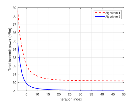
Figure 2: Evaluation of the convergence of the proposed Algorithms 1 and 2.

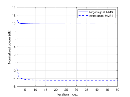
Figure 3: Average receive powers of the target signals and interference for multiple users normalized by noise power versus iteration index.

To shed more light on the properties of Algorithm 2, in Fig. 3, we show the change of normalized receive powers of the target signals and interference during the iterations, where the powers of the target signal and interference for each user are normalized by noise power, i.e., the average values of $A_{k,k}p_{k}/b_{k}$ and $\sum_{q=1,q\neq k}^{K}A_{k,q}p_{q}/b_{k}$ in (17). During the iterations, the normalized signal power decreases by 1 dB, which is mainly caused by the decreasing transmit power of the users. In comparison, the normalized interference power is reduced by more than 3 dB. The results indicate that the positioning optimization for MAs of the users can effectively decrease the correlation of the channel vectors, which contributes to more effectively mitigating the interference among multiple users. It is foreseeable that if sufficient DoFs are available for moving antennas such that the channel vectors of users are orthogonal to each other, the MRC will become the optimal combining at the BS for each user to maximize the effective channel gain without inducing any interference. In practical communication systems with limited space/DoFs, the MAs of users can still be moved within a local region for reshaping the MAC matrix and improving the communication performance.

IV-C Performance Comparison with Benchmark Schemes

Next, we compare the performance of the proposed algorithms with benchmark schemes. Fig. 5 shows the total transmit powers of different schemes versus minimum-achievable-rate requirements for the users. We can observe that the proposed MA solutions outperform FPA and MCP schemes under both ZF and MMSE combining, especially for a large achievable-rate requirement. If the rate requirement is small, the proposed MA-MMSE solution achieves significantly lower transmit power than the MA-ZF scheme. This is because for small $r$, the SINR of each user is more dominantly affected by the noise. The noise amplification caused by ZF combining may deteriorate the SINR performance compared to MMSE combining. As the rate requirement increases, the MA-ZF scheme can approach the performance achieved by MA-MMSE. Besides, we can find that the proposed MA-MMSE solution has a similar performance to the FPA-MMSE and MCP-MMSE schemes for small rate requirements because the interference mitigation acquired by MA positioning optimization has a relatively small influence on the SINR performance if the BS receiver operates in low-SNR regions. However, as the rate requirement increases to be larger than 2 bps/Hz, the performance gap between the proposed MA-MMSE and FPA-MMSE/MCP-MMSE schemes becomes larger. For sufficiently large $r$, the MA-MMSE and MA-ZF solutions can reap 10 dB power-saving compared to other benchmark schemes. The results demonstrate that the MA-enhanced multiuser system can obtain higher performance gain than its counterpart of FPA because of the increasing interference mitigation gain. Moreover, the FPA and MCP schemes have almost the same performance under both ZF and MMSE combining methods. This indicates that the performance gain of MA-enabled multiple access systems is mainly achieved by decreasing the multiuser interference rather than increasing the channel power gain of each user.

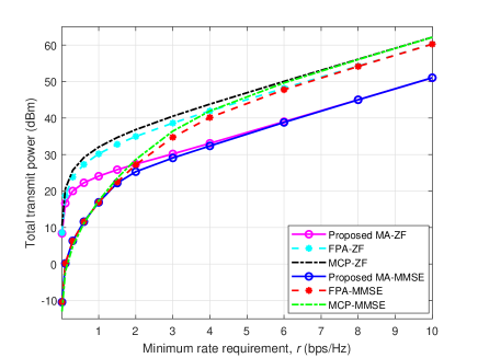
Figure 4: Total transmit powers of different schemes versus minimum-achievable-rate requirements for multiple users.

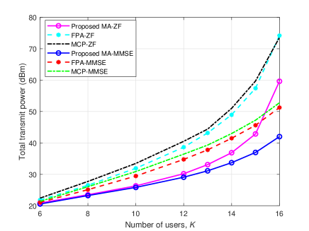
Figure 5: Total transmit powers of different schemes versus the numbers of users.

In Fig. 5, we compare the total transmit powers of different schemes versus the numbers of users. As can be observed, the total transmit power increases with the number of users for all schemes. The reason is as follows. On one hand, each user needs to send signals to the BS for satisfying its rate requirement, which increases the total transmit power. On the other hand, the increasing number of users results in higher interference for MAC, and thus each user has to increase its transmit power for fulfilling its SINR requirement. If the number of users is small, the multiuser interference at the BS receiver can be satisfactorily suppressed by ZF or MMSE combining, and thus the performance gain provided by MA positioning is not significant. As $K$ increases to be close to the number of antennas at the BS, the interference among multiple users cannot be ideally canceled by receive combining because the correlation of the users’ channel vectors is large. In such cases, the positioning optimization of MAs can significantly decrease the correlation of the channel vectors, which is helpful to mitigate multiuser interference. For example, the MA-MMSE solution can save more than 20 dB of transmit power compared to the FPA-MMSE scheme for $K=16$. Moreover, as the number of users increases, the MCP-ZF and MCP-MMSE schemes always achieve a performance worse than other strategies. This indicates that the greedy increase in the channel power gain for each user when optimizing its MA position cannot help mitigating the multiuser interference. From the results in Fig. 5, we know that the MA-enabled multiple access systems can obtain higher interference mitigation gain over conventional FPA systems for a large number of users.

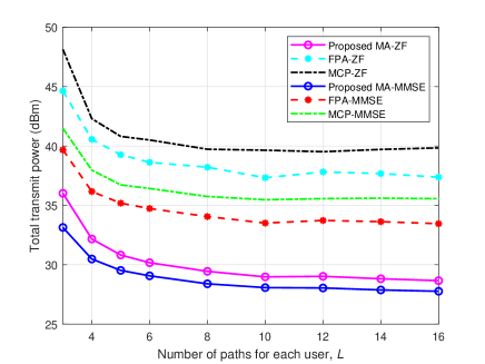
Figure 6: Total transmit powers of different schemes versus the numbers of channel paths for each user.

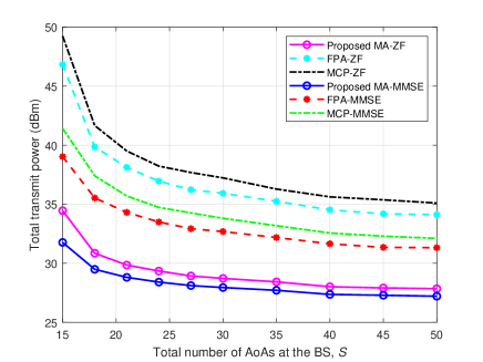
Figure 7: Total transmit powers of different schemes versus the total numbers of AoAs at the BS.

Furthermore, Figs. 7 and 7 show the total transmit powers of different schemes versus the numbers of channel paths for each user and the total numbers of AoAs at the BS, respectively. We can observe again that the total transmit power of MA systems is much smaller than those of FPA and MCP schemes because of the interference mitigation gain provided by MA positioning optimization. Besides, the total transmit powers of the proposed and benchmark schemes all decrease with $L$ and $S$. The reason is as follows. As the number of channel paths for each user increases, the spatial diversity is improved in the transmit/receive region, and thus the correlation among the channel vectors for multiple users decreases. Meanwhile, the MA systems can leverage the prominent channel variation to further decrease the correlation of the MAC. However, as shown in Fig. 7, if $L$ increases to values larger than 8, the descent rate for the total transmit power becomes small. This is because the correlation of channel vectors for multiple users is limited by the number of AoAs at the BS. According to the channel model in (4), the channel vector of user $k$ is a linear combination of the column vectors in receive FRM $\mathbf{F}_{k}$, where the MA positioning optimization can only change the coefficients of linear combinations. If the total number of AoAs of channel paths for multiple users is limited at the BS side, the FRMs of multiple users have similar column vectors. Thus, the local movement of MAs cannot significantly decrease the MAC correlation. On the contrary, as the total number of AoAs at the BS increases, it becomes easier to decrease the channel correlation among multiple users by moving the antennas.

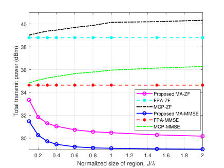
Figure 8: Total transmit powers of different schemes versus normalized region sizes for moving antennas at the users.

In Fig. 8, we compare the total transmit powers of different schemes versus normalized region sizes for moving antennas at the users, where the size of the moving region is normalized by carrier wavelength, i.e., $J/\lambda$. As can be observed, the total transmit powers achieved by MA systems decrease with the normalized size of the moving region and are much smaller than those of FPA and MCP schemes. Moreover, we can see that the total transmit powers of the proposed MA-ZF and MA-MMSE solutions both rapidly decrease as the size of the moving region increases from $0.1\lambda$ to $\lambda$, and achieve their lower bounds for $J=2\lambda$. The results mean that the MA-enabled multiple access systems can even acquire considerable performance gain by moving the antennas of users in a small local region. For example, for communication systems operating at 28 GHz, the volume of a cube of size $2\lambda\times 2\lambda\times 2\lambda$ is about $8\times 10^{-6}~{}\text{m}^{3}$, which is implementable in a small device. In addition, we can observe that the MCP schemes achieve higher transmit power as $J$ increases. This indicates that the greedy maximization of the channel power gain for each user may increase the MAC correlation and deteriorate the overall performance.

IV-D Impact of Imperfect FRI

The above simulation results are based on the assumption that the BS has a perfect knowledge on the FRI, including the AoDs, AoAs, and PRMs of the channel paths between the BS and users. However, in a real-world communication system, the acquisition of FRI requires to send/receive training pilots and feedback between the transceiver. Due to the existence of noise and the limited training overhead, it is challenging to acquire perfect FRI in practice. Thus, it is important to evaluate the impact of imperfect FRI on the performance of MA-enabled multiple access systems. To this end, we introduce two factors to depict the FRI error. On one hand, the AoD error is defined as the difference between the actual and estimated AoDs. Specifically, let $\hat{\vartheta}_{k,j}^{\mathrm{t}}$, $\hat{\varphi}_{k,j}^{\mathrm{t}}$, and $\hat{\omega}_{k,j}^{\mathrm{t}}$ denote the estimated AoDs of the $j$-th channel path between the BS and user $k$, $1\leq k\leq K$, $1\leq j\leq L$. The differences between the estimated and actual AoDs are assumed to be random variables following uniform distributions, i.e., $\vartheta_{k,j}^{\mathrm{t}}-\hat{\vartheta}_{k,j}^{\mathrm{t}}\sim\mathcal{U}[-\mu/2,\mu/2$], $\varphi_{k,j}^{\mathrm{t}}-\hat{\varphi}_{k,j}^{\mathrm{t}}\sim\mathcal{U}[-\mu/2,\mu/2$], and $\omega_{k,j}^{\mathrm{t}}-\hat{\omega}_{k,j}^{\mathrm{t}}\sim\mathcal{U}[-\mu/2,\mu/2$], where $\mu$ denotes the maximum AoD error. On the other hand, the PRM error is defined as the difference between the actual and estimated PRMs. Specifically, let $\hat{\mathbf{\Sigma}}_{k}=\operatorname{diag}\{\hat{\sigma_{1}},\hat{\sigma_{2}},\cdots,\hat{\sigma_{L}}\}$ denote the estimated PRM between the BS and user $k$, $1\leq k\leq K$. Considering the estimation error, the difference between the estimated and actual elements in the PRM is assumed to be a CSCG random variable, i.e., $\frac{\sigma_{j}-\hat{\sigma_{j}}}{|\hat{\sigma_{j}}|}\sim\mathcal{CN}(0,\nu)$, $1\leq j\leq L$, where $\nu$ is the variance of the normalized PRM error.

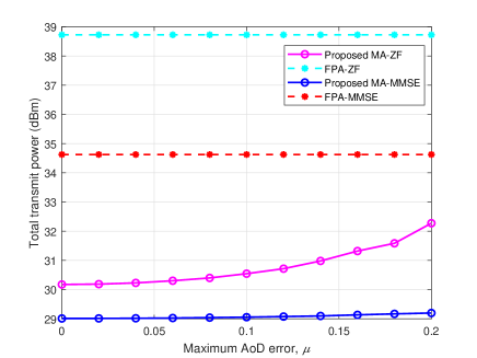
Figure 9: Impact of the AoD error on the performance of the proposed algorithms for MA-enabled multiple access systems.

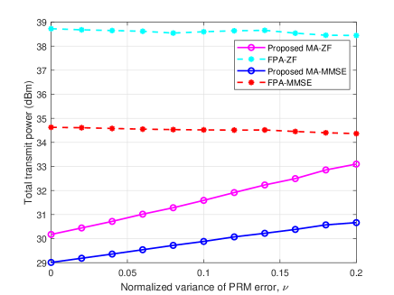
Figure 10: Impact of the PRM error on the performance of the proposed algorithms for MA-enabled multiple access systems.

In Fig. 10, we evaluate the impact of the AoD error on the performance of the proposed algorithms for MA-enabled multiple access systems, where the AoAs of the channel paths and the PRMs between the BS and users are assumed to be known for optimization. In the simulation, the MA positioning optimization is executed based on the estimated (imperfect) FRI. After the MAs are deployed at target positions, the combining matrix at the BS and the transmit power of users are calculated based on the actual channel vectors between the BS and users. As can be observed in Fig. 10, the total transmit power slightly increases with the maximum AoD error because of the deviation between the estimated and actual channels. However, the performance gap between the FPA and MA systems is still significant even for large values of $\mu$. Besides, the proposed MA-MMSE solution is robust to the AoD error, where the performance loss for $\mu=2$ is negligible compared to the perfect FRI case, i.e., not exceeding 0.2 dB power increment. The reason is as follows. Since the size of the region for moving antenna is no larger than $2\lambda$, the deviation of transmit FRVs for estimated and actual AoDs is not significant for a small AoD error. Thus, the MA positioning optimization based on estimated AoDs and transmit FRVs can still yield a good performance for the channels with actual AoDs.

Finally, Fig 10 evaluates the impact of the PRM error on the performance of the proposed algorithms for MA-enabled multiple access systems, where the AoAs and AoDs of the channel paths between the BS and users are assumed to be known for optimization. Similar to Fig. 10, in the simulation, the MA positioning optimization is executed based on the estimated FRI, while the combining matrix at the BS and the transmit power of users are calculated based on the actual channel vectors between the BS and users. We can observe again that the total transmit power increases with the variance of normalized PRM error due to the inaccurate channel information for MA positioning optimization. As $\nu$ increases from 0 to 0.2, the total transmit powers of the users for MA-ZF and MA-MMSE solutions are increased by 2.9 dB and 1.6 dB, respectively. However, the superiority of the proposed MA schemes over conventional FPA schemes is still significant even for a large value of $\nu$. It is worth noting that the normalized mean square error (MSE) of the estimated PRM is approximately equal to our defined variance of normalized PRM error, i.e., $\|\mathbf{\Sigma}_{k}-\hat{\mathbf{\Sigma}}_{k}\|_{\mathrm{F}}^{2}/\|\mathbf{\Sigma}_{k}\|_{\mathrm{F}}^{2}\approx\nu$. Thus, $\nu=0.2$ indicates a poor condition under which the estimation errors are very close to the values of elements in PRM. In this regard, the proposed MA positioning solutions are shown to be robust to the PRM error.

V Conclusion

In this paper, we investigated the MA-enhanced MAC for the uplink transmission from multiple users equipped with a single MA to a BS equipped with an FPA array. A field-response based channel model was used to characterize the multi-path channel vector between the antenna array of the BS and each user’s MA with a flexible position. Then, we formulated an optimization problem for minimizing the total transmit power of users by jointly optimizing the positions of MAs and the transmit power of users, as well as the receive combining matrix of the BS, subject to a minimum-achievable-rate requirement for each user. Since the resultant problem is highly non-convex and involves coupled variables, we developed two algorithms based on ZF and MMSE combining methods, respectively, where the combining matrix of the BS and the total transmit power of users are expressed as a function of the MA positioning vector during the iterations. For each iteration, the MA positioning vector is updated by using the gradient descent method, where the step size is obtained via backtracking line search. Analytical results showed that the proposed ZF-based and MMSE-based algorithms for MA-enabled multiple access systems can converge to suboptimal solutions with low computational complexities. Besides, an alternative solution for the single-user case was also provided, where the power-minimization problem is equivalent to maximizing the channel gain of the user. Extensive simulations were carried out to verify the superiority of the proposed MA-enabled multiple access systems. It was shown that the proposed MA-ZF and MA-MMSE solutions can significantly decrease the total transmit power of users as compared to conventional FPA systems. Especially for the scenarios with a large number of users and/or high achievable-rate requirements, the interference mitigation gain provided by MA positioning optimization becomes more significant. Besides, the results revealed that the increasing number of channel paths and the increasing size of the region for moving antennas can help decrease the total transmit power of users. Moreover, we evaluated the impact of imperfect FRI on the solution for MA positioning. It was shown that the proposed algorithms can achieve a robust performance against AoD and PRM errors.

A natural generalization of this work is to consider multi-MA users and/or multi-cell systems. In such scenarios, the coordination of user precoding and its joint optimization with receive combining and MA positioning should be studied. Besides, FRI plays an important role in MA-enabled communication systems, where the AoDs, AoAs, and PRMs should be known to the BS for joint optimization. Thus, efficient FRI estimation protocols and algorithms are required to achieve a good tradeoff between the training overhead and communication performance. These aspects are interesting topics for future research.

According to the definition of channel vector in (4), the objective function in (31a) can be written as

$$\left\|\mathbf{h}(\mathbf{u})\right\|_{2}^{2}=\left\|\mathbf{F}^{\mathrm{H}}\mathbf{\Sigma}\mathbf{g}(\mathbf{u})\right\|_{2}^{2}=\mathbf{g}(\mathbf{u})^{\mathrm{H}}\mathbf{\Sigma}^{\mathrm{H}}\mathbf{F}\mathbf{F}^{\mathrm{H}}\mathbf{\Sigma}\mathbf{g}(\mathbf{u})\triangleq\mathbf{g}(\mathbf{u})^{\mathrm{H}}\mathbf{Q}\mathbf{g}(\mathbf{u}),$$ (32)

where $\mathbf{F}\in\mathbb{C}^{L^{\mathrm{r}}\times N}$ and $\mathbf{\Sigma}\in\mathbb{C}^{L^{\mathrm{t}}\times L^{\mathrm{r}}}$ are the receive FRM and PRM between the BS and user, respectively. $L^{\mathrm{t}}$ and $L^{\mathrm{r}}$ represent the number of transmit and receive channel paths, respectively. $\mathbf{g}(\mathbf{u})=\left[e^{\mathrm{j}\frac{2\pi}{\lambda}\rho_{1}^{\mathrm{t}}(\mathbf{u})},e^{\mathrm{j}\frac{2\pi}{\lambda}\rho_{2}^{\mathrm{t}}(\mathbf{u})},\cdots,e^{\mathrm{j}\frac{2\pi}{\lambda}\rho_{L^{\mathrm{t}}}^{\mathrm{t}}(\mathbf{u})}\right]^{\mathrm{T}}$ is the transmit FRV at the user, with $\rho_{j}^{\mathrm{t}}(\mathbf{u})=x\vartheta_{j}^{\mathrm{t}}+y\varphi_{j}^{\mathrm{t}}+z\omega_{j}^{\mathrm{t}}$, $1\leq j\leq L^{\mathrm{t}}$.

Denoting the entry in the $m$-th row and $n$-th column of matrix $\mathbf{Q}$ as $q_{m,n}$, $1\leq m,n\leq L^{\mathrm{t}}$, the partial derivative of (32) w.r.t. $x$ is given by

$$\frac{\partial\mathbf{g}(\mathbf{u})^{\mathrm{H}}\mathbf{Q}\mathbf{g}(\mathbf{u})}{\partial x}=\frac{\partial\sum\limits_{m=1}^{L^{\mathrm{t}}}\sum\limits_{n=1}^{L^{\mathrm{t}}}q_{m,n}\mathrm{e}^{\mathrm{j}\frac{2\pi}{\lambda}\left[\rho_{n}^{\mathrm{t}}(\mathbf{u})-\rho_{m}^{\mathrm{t}}(\mathbf{u})\right]}}{\partial x}$$ (33)

$$= \frac{\partial\sum\limits_{m=1}^{L^{\mathrm{t}}}\sum\limits_{n=1}^{L^{\mathrm{t}}}\Re\{q_{m,n}\}\cos\left[\frac{2\pi}{\lambda}\left(\rho_{n}^{\mathrm{t}}(\mathbf{u})-\rho_{m}^{\mathrm{t}}(\mathbf{u})\right)\right]-\Im\{q_{m,n}\}\sin\left[\frac{2\pi}{\lambda}\left(\rho_{n}^{\mathrm{t}}(\mathbf{u})-\rho_{m}^{\mathrm{t}}(\mathbf{u})\right)\right]}{\partial x}$$

$$= \sum\limits_{m=1}^{L^{\mathrm{t}}}\sum\limits_{n=1}^{L^{\mathrm{t}}}(\vartheta_{m}^{\mathrm{t}}-\vartheta_{n}^{\mathrm{t}})\left\{\Re\{q_{m,n}\}\sin\left[\frac{2\pi}{\lambda}\left(\rho_{n}^{\mathrm{t}}(\mathbf{u})-\rho_{m}^{\mathrm{t}}(\mathbf{u})\right)\right]+\Im\{q_{m,n}\}\cos\left[\frac{2\pi}{\lambda}\left(\rho_{n}^{\mathrm{t}}(\mathbf{u})-\rho_{m}^{\mathrm{t}}(\mathbf{u})\right)\right]\right\}$$

$$= \sum\limits_{m=1}^{L^{\mathrm{t}}}\sum\limits_{n=1}^{L^{\mathrm{t}}}(\vartheta_{m}^{\mathrm{t}}-\vartheta_{n}^{\mathrm{t}})|q_{m,n}|\sin\left[\frac{2\pi}{\lambda}\left(\rho_{n}^{\mathrm{t}}(\mathbf{u})-\rho_{m}^{\mathrm{t}}(\mathbf{u})\right)+\angle\{q_{m,n}\}\right].$$

Similarly, the partial derivatives of (32) w.r.t. $y$ and $z$ are respectively given by

$$\frac{\partial\mathbf{g}(\mathbf{u})^{\mathrm{H}}\mathbf{Q}\mathbf{g}(\mathbf{u})}{\partial y}=\sum\limits_{m=1}^{L^{\mathrm{t}}}\sum\limits_{n=1}^{L^{\mathrm{t}}}(\varphi_{m}^{\mathrm{t}}-\varphi_{n}^{\mathrm{t}})|q_{m,n}|\sin\left[\frac{2\pi}{\lambda}\left(\rho_{n}^{\mathrm{t}}(\mathbf{u})-\rho_{m}^{\mathrm{t}}(\mathbf{u})\right)+\angle\{q_{m,n}\}\right],$$ (34)

$$\frac{\partial\mathbf{g}(\mathbf{u})^{\mathrm{H}}\mathbf{Q}\mathbf{g}(\mathbf{u})}{\partial z}=\sum\limits_{m=1}^{L^{\mathrm{t}}}\sum\limits_{n=1}^{L^{\mathrm{t}}}(\omega_{m}^{\mathrm{t}}-\omega_{n}^{\mathrm{t}})|q_{m,n}|\sin\left[\frac{2\pi}{\lambda}\left(\rho_{n}^{\mathrm{t}}(\mathbf{u})-\rho_{m}^{\mathrm{t}}(\mathbf{u})\right)+\angle\{q_{m,n}\}\right].$$ (35)

References

- [1] E. Telatar, “Capacity of multi-antenna gaussian channels,” European Trans. Telecommun., vol. 10, no. 6, pp. 585–595, Nov. 1999.
- [2] A. Paulraj, D. Gore, R. Nabar, and H. Bolcskei, “An overview of MIMO communications - a key to gigabit wireless,” Proc. IEEE, vol. 92, no. 2, pp. 198–218, Feb. 2004.
- [3] G. Stuber, J. Barry, S. McLaughlin, Y. Li, M. Ingram, and T. Pratt, “Broadband MIMO-OFDM wireless communications,” Proc. IEEE, vol. 92, no. 2, pp. 271–294, Feb. 2004.
- [4] E. G. Larsson, O. Edfors, F. Tufvesson, and T. L. Marzetta, “Massive MIMO for next generation wireless systems,” IEEE Commun. Mag., vol. 52, no. 2, pp. 186–195, Feb. 2014.
- [5] L. Lu, G. Y. Li, A. L. Swindlehurst, A. Ashikhmin, and R. Zhang, “An overview of massive MIMO: Benefits and challenges,” IEEE J. Sel. Topics Signal Process., vol. 8, no. 5, pp. 742–758, Oct. 2014.
- [6] Y. Zeng and R. Zhang, “Millimeter wave MIMO with lens antenna array: A new path division multiplexing paradigm,” IEEE Trans. Commun., vol. 64, no. 4, pp. 1557–1571, Apr. 2016.
- [7] L. Zhu, J. Zhang, Z. Xiao, X. Cao, D. O. Wu, and X.-G. Xia, “Millimeter-wave NOMA with user grouping, power allocation and hybrid beamforming,” IEEE Trans. Wireless Commun., vol. 18, no. 11, pp. 5065–5079, Nov. 2019.
- [8] B. Ning, Z. Tian, Z. Chen, C. Han, S. Li, J. Yuan, and R. Zhang, “A review of beamforming technologies for ultra-massive MIMO in terahertz communications,” arXiv preprint arXiv:2107.03032, 2022.
- [9] L. Zhu, W. Ma, and R. Zhang, “Modeling and performance analysis for movable antenna enabled wireless communications,” arXiv preprint arXiv:2210.05325, 2022.
- [10] W. Ma, L. Zhu, and R. Zhang, “MIMO capacity characterization for movable antenna systems,” arXiv preprint arXiv:2210.05396, 2022.
- [11] D. Castanheira and A. Gameiro, “Distributed antenna system capacity scaling,” IEEE Wireless Commun., vol. 17, no. 3, pp. 68–75, Jun. 2010.
- [12] R. Heath, S. Peters, Y. Wang, and J. Zhang, “A current perspective on distributed antenna systems for the downlink of cellular systems,” IEEE Commun. Mag., vol. 51, no. 4, pp. 161–167, Apr. 2013.
- [13] H. Cui and Y. Liu, “Green distributed antenna systems for smart communities: A comprehensive survey,” China Commun., vol. 16, no. 11, pp. 70–80, Nov. 2019.
- [14] A. Zhuravlev, V. Razevig, S. Ivashov, A. Bugaev, and M. Chizh, “Experimental simulation of multi-static radar with a pair of separated movable antennas,” in Proc. IEEE International Conf. Microwaves Commun. Antennas Electron. Syst. (COMCAS), Nov. 2015, pp. 1–5.
- [15] S. Basbug, “Design and synthesis of antenna array with movable elements along semicircular paths,” IEEE Antennas Wireless Propagat. Lett., vol. 16, pp. 3059–3062, Oct. 2017.
- [16] K.-K. Wong, A. Shojaeifard, K.-F. Tong, and Y. Zhang, “Fluid antenna systems,” IEEE Trans. Wireless Commun., vol. 20, no. 3, pp. 1950–1962, Mar. 2021.
- [17] K.-K. Wong and K.-F. Tong, “Fluid antenna multiple access,” IEEE Trans. Wireless Commun., vol. 21, no. 7, pp. 4801–4815, Jul. 2022.
- [18] Z. Chai, K.-K. Wong, K.-F. Tong, Y. Chen, and Y. Zhang, “Port selection for fluid antenna systems,” IEEE Commun. Lett., vol. 26, no. 5, pp. 1180–1184, May 2022.
- [19] M. Khammassi, A. Kammoun, and M.-S. Alouini, “A new analytical approximation of the fluid antenna system channel,” arXiv preprint arXiv:2203.09318, 2022.
- [20] K. N. Paracha, A. D. Butt, A. S. Alghamdi, S. A. Babale, and P. J. Soh, “Liquid metal antennas: Materials, fabrication and applications,” Sensors, vol. 20, no. 1, pp. 1–26, 2019.
- [21] J. Dong, Y. Zhu, Z. Liu, and M. Wang, “Liquid metal-based devices: Material properties, fabrication and functionalities,” Nanomaterials, vol. 11, no. 12, pp. 1–29, 2021.
- [22] A. M. Morishita, C. K. Kitamura, A. T. Ohta, and W. A. Shiroma, “A liquid-metal monopole array with tunable frequency, gain, and beam steering,” IEEE Antennas Wireless Propagat. Lett., vol. 12, pp. 1388–1391, Oct. 2013.
- [23] H. Boche and M. Schubert, “A general duality theory for uplink and downlink beamforming,” in Proc. IEEE Veh. Technol. Conf., vol. 1, Sep. 2002, pp. 87–91.
- [24] S. Vishwanath, N. Jindal, and A. Goldsmith, “Duality, achievable rates, and sum-rate capacity of gaussian MIMO broadcast channels,” IEEE Trans. Inform. Theory, vol. 49, no. 10, pp. 2658–2668, Oct. 2003.
- [25] W. Yu, “Uplink-downlink duality via minimax duality,” IEEE Trans. Inform. Theory, vol. 52, no. 2, pp. 361–374, Feb. 2006.
- [26] D. Tse and P. Viswanath, Fundamentals of Wireless Communication. New York, USA: Cambridge Univ. Press, 2005.
- [27] E. K. Chong and S. H. Zak, An introduction to optimization. Hoboken, New Jersey, USA: John Wiley & Sons, 2013.
- [28] S. Boyd and L. Vandenberghe, Convex Optimization. Cambridge, U.K.: Cambridge Univ. Press, 2004.