Investigating Multi-source Active Learning for Natural Language Inference

Abstract

In recent years, active learning has been successfully applied to an array of NLP tasks. However, prior work often assumes that training and test data are drawn from the same distribution. This is problematic, as in real-life settings data may stem from several sources of varying relevance and quality. We show that four popular active learning schemes fail to outperform random selection when applied to unlabelled pools comprised of multiple data sources on the task of natural language inference. We reveal that uncertainty-based strategies perform poorly due to the acquisition of collective outliers, i.e., hard-to-learn instances that hamper learning and generalization. When outliers are removed, strategies are found to recover and outperform random baselines. In further analysis, we find that collective outliers vary in form between sources, and show that hard-to-learn data is not always categorically harmful. Lastly, we leverage dataset cartography to introduce difficulty-stratified testing and find that different strategies are affected differently by example learnability and difficulty.

1 Introduction

In recent years, active learning (AL) Cohn et al. (1996) has emerged as a promising avenue for data-efficient supervised learning Zhang et al. (2022). AL has been successfully applied to a variety of NLP tasks, such as text classification (Zhang et al., 2016; Siddhant and Lipton, 2018; Prabhu et al., 2019; Ein-Dor et al., 2020; Margatina et al., 2022), entity recognition (Shen et al., 2017; Siddhant and Lipton, 2018; Lowell et al., 2019), part-of-speech tagging Chaudhary et al. (2021) and neural machine translation (Peris and Casacuberta, 2018; Liu et al., 2018; Zhao et al., 2020).

However, these works share a major limitation: they often implicitly assume that unlabelled training data comes from a single source (Houlsby et al., 2011; Sener and Savarese, 2018; Huang et al., 2016; Gissin and Shalev-Shwartz, 2019; Margatina et al., 2021). We refer to this setting as single-source AL.

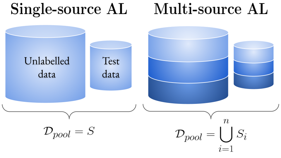
Figure 1: The pool of unlabelled data consists of a source $S$, or multiple sources $\bigcup_{i}S_{i}$, for the single-source and multi-source AL setting, respectively. The in-domain test set follows the same distribution of sources.

The single-source assumption is problematic for various reasons Kirsch et al. (2021). In real-life settings we have no guarantees that all unlabelled data at our disposal will necessarily stem from the same distribution, nor will we have assurances that all examples are of consistent quality, or that they bear sufficient relevancy to our task. For instance, quality issues may arise when unlabelled data is collected through noisy processes with limited room for monitoring individual samples, such as web-crawling Kreutzer et al. (2022). Alternatively, one may have access to several sources of unlabelled data of decent quality, but incomplete knowledge of their relevance to the task-at-hand. For instance, medical data may be collected from various different physical sites (hospitals, clinics, general practitioners) which may differ statistically from the target distribution due to e.g., differences in patient demographics. Ideally, AL methods should be robust towards these conditions in order to achieve adequate solutions.

In this work, we study whether existing AL methods can adequately select relevant data points in a multi-source scenario for NLP. We examine robustness by evaluating AL performance in both in-domain (ID) and out-of-domain (OOD) settings, while we also conduct an extensive analysis to interpret our findings. A primary phenomenon of interest here concerns collective outliers: data points which models struggle to learn due to high ambiguity, the requirement of specialist skills or labelling errors Han and Kamber (2000). While such outliers were previously found to disrupt several AL methods for visual question answering Karamcheti et al. (2021), their impact on text-based tasks remains under-explored. Given the wide body of work on the noise and biases that pervade the task of natural language inference (NLI) (Bowman et al., 2015; Williams et al., 2017; Gururangan et al., 2018; Poliak et al., 2018; Tsuchiya, 2018; Geva et al., 2019; Liu et al., 2022), we may reasonably assume popular NLI datasets to suffer from collective outliers as well.

Concretely, our contributions can be summarised as follows: (1) We apply several popular AL methods in the under-explored multi-source, pool-based setting on the task of NLI, using RoBERTa-large (Liu et al., 2020) as our acquisition model, and find that no strategy consistently outperforms random selection (§5). (2) We seek to explain our findings by creating datamaps to explore the actively acquired data (§6.1) and show that uncertainty-based acquisition functions perform poorly due to the acquisition of collective outliers (§6.2). (3) We examine the effect of training data difficulty on downstream performance (§7.1) and after thorough experiments we find that uncertainty-based AL methods recover and even surpass random selection when hard-to-learn data points are removed from the pool (§7.2). (4) Finally, we introduce difficulty-stratified testing and show that the learnability of acquired training data affects different strategies differently at test-time (§7.3). Our code is publicly available at https://github.com/asnijders/multi_source_AL.

2 Related Work

Multi-source AL for NLP

While AL has been studied for a variety of tasks in NLP Siddhant and Lipton (2018); Lowell et al. (2019); Ein-Dor et al. (2020); Shelmanov et al. (2021); Margatina et al. (2021); Yuan et al. (2022); Schröder et al. (2022); Margatina et al. (2022); Kirk et al. (2022); Zhang et al. (2022), the majority of work remains limited to settings where training data is assumed to stem from a single source. Some recent works have sought to address the issues that arise when relaxing the single-source assumption (Ghorbani et al., 2021; Kirsch et al., 2021; Kirsch and Gal, 2021), though results remain primarily limited to image classification. Moreover, these works study how AL fares under the presence of corrupted training data, such as duplicating images or adding Gaussian noise, and they do not consider settings where sampling from multiple sources may be beneficial due to complementary source attributes. He et al. (2021) examine a multi-domain AL setting, but they focus on leveraging common knowledge between domains to learn a set of models for a set of domains, which contrasts with our single-model pool-based setup. Closest to our work, Longpre et al. (2022) explore pool-based AL over multiple domains and find that some strategies consistently outperform random on question answering and sentiment analysis. However, the authors crucially omit a series of measurements, as they instead perform a single AL iteration, limiting the effectiveness of AL, while complicating comparison with our results.

Dataset Cartography

Karamcheti et al. (2021) employ dataset cartography Swayamdipta et al. (2020) and show that a series of AL algorithms fail to outperform random selection in visual question answering due to the presence of collective outliers. Zhang and Plank (2021) apply datamaps to AL and introduce the cartography active learning strategy, identifying that examples with poor learnability often suffer from label errors. Our work contrasts with both of these works in that we show that hard-to-learn data is not always unequivocally harmful to learning. Moreover, both works only examine learnability of training examples, whereas we also consider how learnability of acquired data affects model performance at test-time.

3 Single & Multi-source Active Learning

We assume a warm-start, pool-based AL scenario Settles (2010) with access to a pool of unlabelled training data, $\mathcal{D}_{pool}$, and a seed dataset of labelled examples, $\mathcal{D}_{train}$. During each iteration $i$ of AL, we first train a model $\mathcal{M}$ with $\mathcal{D}_{train}$ and then use it in conjunction with some acquisition function $\mathcal{A}$ to select a new batch of unlabelled examples $\mathcal{D}_{batch}$ from $\mathcal{D}_{pool}$ for labelling. Upon labelling, these examples are removed from $\mathcal{D}_{pool}$ and added to $\mathcal{D}_{train}$, after which a new round of AL begins.

$$\mathcal{D}_{train}^{i+1}=\mathcal{D}_{train}^{i}\cup\mathcal{D}_{batch}^{i+1}$$

$$\mathcal{D}_{pool}^{i+1}=\mathcal{D}_{pool}^{i}\setminus\mathcal{D}_{batch}^{i+1}$$

Single-source AL

For single-source AL, we assume that $\mathcal{D}_{pool}$ is a set of unlabelled data that stems from a single source $S$, i.e. $\mathcal{D}_{pool}=S$.

Multi-source AL

For multi-source AL, we assume that $\mathcal{D}_{pool}$ comprises a union of distinct sources $S_{1},S_{2},...,S_{n}$ such that $\mathcal{D}_{pool}=\bigcup\limits_{i=1}^{n}S_{i}$.

3.1 Data Acquisition

An acquisition function $\mathcal{A}$ is responsible for selecting the most informative unlabelled data from the pool, aiming to improve over random sampling. We use a set of acquisition functions which we deem representative for the wider AL toolkit: Monte Carlo Dropout Max-Entropy, (mcme; Gal et al., 2017) is an uncertainty-based acquisition strategy where we take the mean label distribution over $T$ Monte-Carlo dropout (Gal and Ghahramani, 2015) network samples and select the $k$ data points with the highest predictive entropy. Bayesian Active Learning by Disagreement, (bald; Houlsby et al., 2011) is an uncertainty-based acquisition strategy which employs Bayesian uncertainty to identify data points for which many models disagree about. Discriminative Active Learning (dal; Gissin and Shalev-Shwartz, 2019) is a diversity-based acquisition function designed to acquire a training set that is indistinguishable from the unlabelled set.

3.2 Analysis of Acquired Data

At each data acquisition step, we seek to examine what kind of data each acquisition function has selected for annotation. Following standard practice in active learning literature (Zhdanov, 2019; Yuan et al., 2020; Ein-Dor et al., 2020; Margatina et al., 2021) we profile datasets acquired by strategies via acquisition metrics. Concretely, we consider the input diversity and output uncertainty metrics. We provide more details in Appendix 9.1.

Input Diversity

To evaluate the diversity of acquired sets in the input space, we follow Yuan et al. (2020) and measure input diversity as the Jaccard similarity between the set of tokens from the acquired training set $\mathcal{D}_{train}$ and the set of tokens from the remainder of the unlabelled pool $\mathcal{D}_{pool}$. This function assigns high diversity to strategies acquiring samples with high token overlap with the unlabelled pool, and vice versa.

Output Uncertainty

To approximate the output uncertainty of an acquired training set $\mathcal{D}_{train}$ for a given strategy, we follow Yuan et al. (2020) and use a model trained on the entire dataset to compute predictive entropy of all the examples in the dataset that we want to examine. The model is trained on all training data as this grants more accurate uncertainty measurements.

4 Experimental Setup

Data

We perform experiments on Natural Language Inference (NLI), a popular classification task to gauge a model’s natural language understanding (Bowman et al., 2015). We construct the unlabelled pool from three distinct datasets: snli (Bowman et al., 2015), anli (Nie et al., 2019) and wanli (Liu et al., 2022). We consider mnli (Williams et al., 2017) as an out-of-domain set to evaluate the transferability of actively acquired training sets. For more details see Appendix 9.2.

Experiments

We apply AL with two distinct end-goals: in-domain (ID) generalization, where the same source(s) are used for both the unlabelled pool $\mathcal{D}_{pool}$ and the test set $\mathcal{D}_{test}$, and out-of-domain (OOD) generalization, where we evaluate on the test set of an external source of which no training data was present in the unlabelled pool.

Constructing multi-source pools

For multi-source AL, the unlabelled pool comprises the union of the snli, anli and wanli training sets. During model selection, we similarly assume the union of snli, anli and wanli validation sets. For both training and validation data we down-sample sources to the minority source size to obtain pools with even shares per source. We sub-sample training data for each source to reduce experiment runtimes. This yields a pool of $60$K unlabelled training examples comprised of $20$K shares of each source.

AL Parameters

We assume an initial seed training set of size $|\mathcal{D}_{train}^{i=0}|=500$ and an acquisition size $k=500$, such that $k$ examples are acquired per round of AL. We perform $7$ rounds of AL: the final actively acquired labelled dataset $\mathcal{D}_{train}^{i=7}$ comprises $4$K examples. We run each experiment $5$ times with different random seeds to account for stochasticity in parameter initializations.

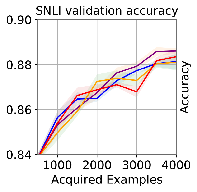
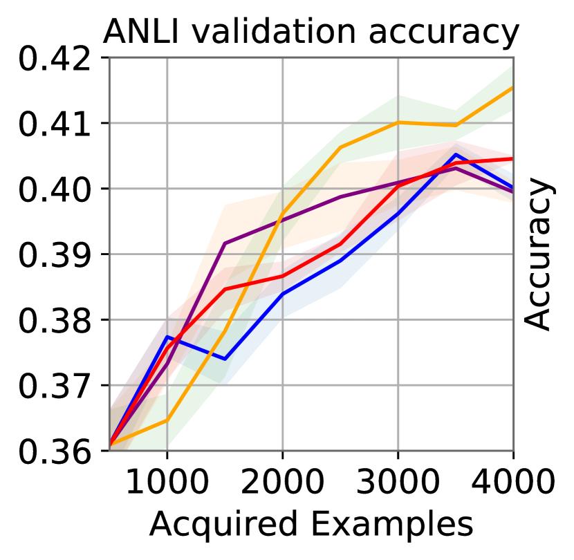
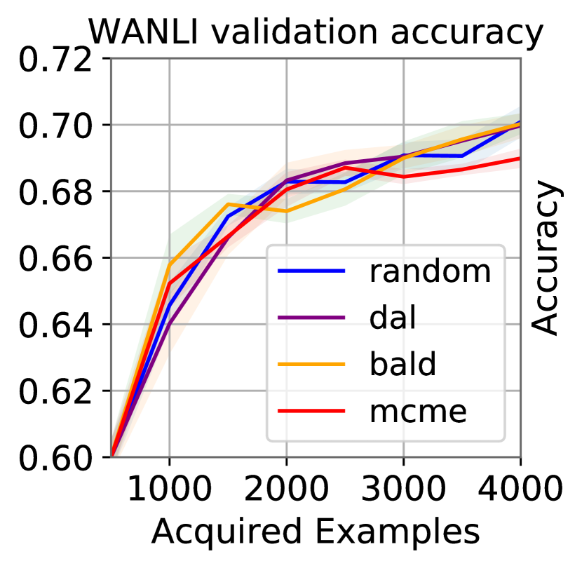
Figure 2: AL single-source in-domain learning curves.

5 Results

5.1 AL over single sources

We first provide single-source AL results in Figure 2. AL has mixed performance across sources; it fails to consistently outperform random selection on snli and wanli, though most strategies tend to outperform random on anli. However, none of the strategies consistently outperform others across sources. Moreover, the extent of improvement over the acquisition phase varies between tasks; e.g., for snli, strategy curves are close and the accuracy improvement from $500$ to $4$K examples is small. This is also reflected in test outcomes (Table 1), with models performing similarly across sources.

Observing Table 2, we find that uncertainty-based methods (bald, mcme) tend to acquire the most uncertain data points, as expected. Still, differences between strategies are small for wanli and anli. Conversely, random and dal tend to acquire data with greater diversity in the input space, but again variance across methods is low. Here, observed homogeneity in the input space may explain why test outcomes lie closely together: if the acquired training sets per strategy are very similar, we should expect to see similarly small differences in test outcomes for models trained on them. Relating these outcomes to the per-source learning curves in Figure 2, however, we observe no clear relation between metric results and performance outcomes: acquiring uncertain or diverse data does not seem to be predictive of AL success throughout the acquisition process.

	snli	anli	wanli
random	$87.09\pm 0.30$	$39.90\pm 1.02$	$\textbf{70.24}\pm 0.70$
dal	$87.49\pm 0.20$	$39.84\pm 1.15$	$69.80\pm 1.00$
bald	$87.37\pm 0.40$	$\textbf{40.16}\pm 0.69$	$69.54\pm 0.70$
mcme	$\textbf{87.58}\pm 0.80$	$40.15\pm 0.60$	$69.07\pm 1.20$

Table 1: Single-source AL test results. At test-time, the labeled set $\mathcal{D}_{train}$ comprises $4$K examples.

Task	Strategy	I-Div.	Unc.	N	E	C
	random	$0.259$	$0.051$	0.34	0.33	0.33
snli	dal	0.267	$0.067$	0.38	0.29	0.33
	bald	$0.249$	$0.072$	0.32	0.31	0.37
	mcme	$0.261$	0.093	0.32	0.34	0.34
	random	0.324	$0.208$	0.47	0.38	0.15
wanli	dal	$0.321$	$0.223$	0.49	0.38	0.13
	bald	$0.317$	$0.213$	0.40	0.39	0.21
	mcme	$0.318$	0.229	0.38	0.35	0.27
	random	0.492	$0.082$	0.43	0.32	0.26
anli	dal	$0.467$	$0.084$	0.47	0.3	0.23
	bald	$0.478$	$0.094$	0.39	0.30	0.31
	mcme	$0.491$	0.110	0.37	0.31	0.31
	random	$0.276$	$0.405$	0.41	0.34	0.25
Multi	dal	$0.276$	$0.463$	0.47	0.34	0.19
	bald	$0.220$	$0.445$	0.34	0.32	0.35
	mcme	0.323	0.556	0.40	0.30	0.30

Table 2: Profiling strategy acquisitions for single-source and multi-source AL in terms of input diversity (I-Div.), uncertainty (Unc.) and class distributions (N: neutral, E: entailment, C: contradiction) across seeds. Each strategy is profiled after all rounds of AL.

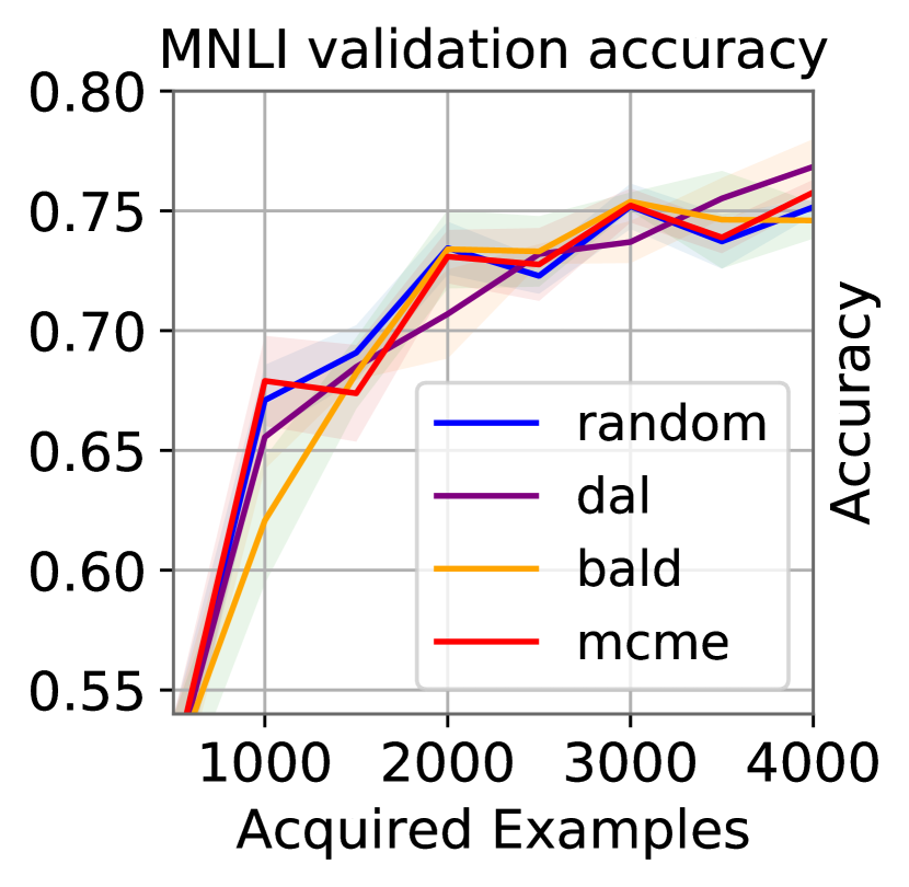
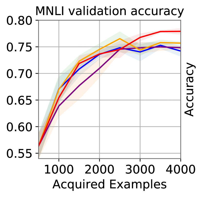
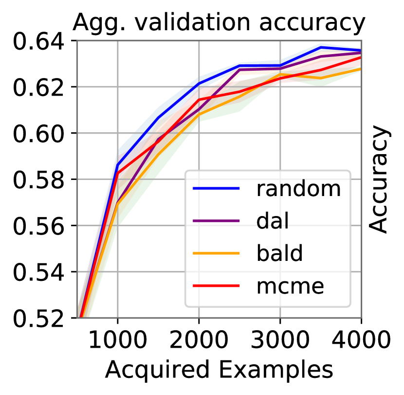
(a) Original training data

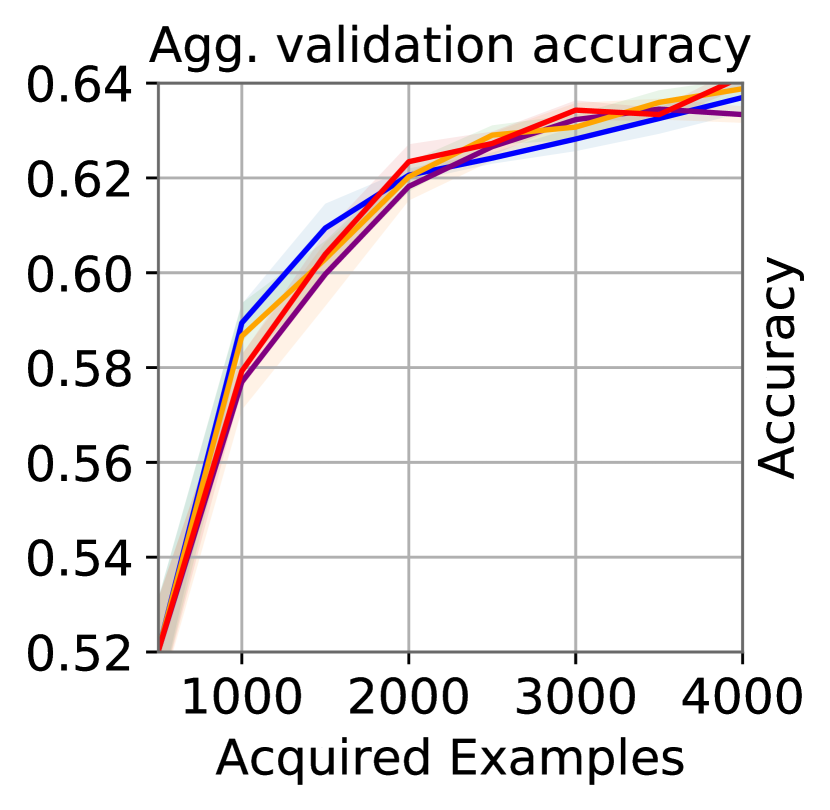
(b) Hard-to-learn removed

Figure 3: Multi-source AL OOD (mnli) and ID (snli, anli, wanli) learning curves. On the left, the unlabelled pool has been left untreated; on the right, hard-to-learn data was removed from the pool.

	snli	anli	wanli	mnli
random	$85.9\pm 0.9\mid 85.3\pm 0.3$	$37.8\pm 1.2\mid 37.9\pm 0.8$	$67.7\pm 1.6\mid 67.2\pm 0.9$	$74.2\pm 2.3\mid 74.4\pm 1.5$
mcme	$85.9\pm 0.7\mid 84.3\pm 0.6$	$\underline{\textbf{38.6}}\pm 1.0\mid\underline{38.4}\pm 0.9$	$67.4\pm 0.4\mid 66.3\pm 0.7$	$\underline{\textbf{77.8}}\pm 1.3\mid 75.6\pm 2.2$
bald	$\underline{\textbf{86.3}}\pm 1.0\mid\underline{85.8}\pm 0.2$	$36.9\pm 1.3\mid 36.1\pm 0.5$	$\underline{\textbf{68.4}}\pm 1.1\mid 65.9\pm 1.1$	$75.8\pm 0.9\mid 74.3\pm 1.6$
dal	$84.3\pm 1.2\mid 85.3\pm 0.9$	$37.8\pm 1.2\mid 37.3\pm 1.3$	$68.0\pm 0.6\mid\underline{68.1}\pm 1.0$	$74.6\pm 1.2\mid\underline{76.6}\pm 2.6$

Table 3: Multi-source AL test outcomes with and without hard-to-learn instances removed. Cell scheme to be read as ablated $\mid$ original. Bold denotes best score for each test set overall and underline best score per setting. At test-time, the labeled set $\mathcal{D}_{train}$ comprises $4$K examples.

5.2 AL over multiple sources

Next, we provide the results of our multi-source setting, as described in §3, and observe that again AL fails to consistently outperform random sampling on the aggregate ID test set of snli, anli and wanli (Figure 3, bottom left). We also evaluate on the OOD mnli that was not present in the unlabelled training data (Figure 3, top left) and still find that AL fails to outperform random.

Analyzing the acquired data in terms of input diversity, uncertainty and label distributions (Table 2) There do not appear to be clear relations between metric outcomes and strategy performance otherwise, i.e., acquiring diverse or uncertain batches does not seem to lead to higher performance.

6 Dataset Cartography for AL Diagnosis

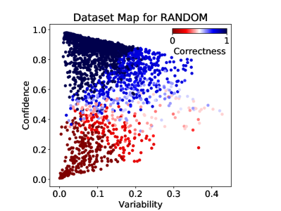
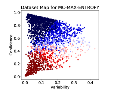
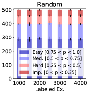
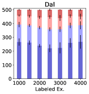
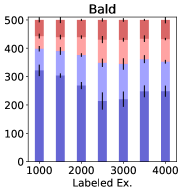
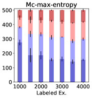
Figure 4: Top row: Strategy maps for random and mcme for multi-source AL. Correctness denotes how often the model predicts the correct label. Bottom row: Acquisition by difficulty over time for random, dal, bald and mcme. We provide additional datamap plots in the appendix (Section 9.5).

Our findings in both single and multi-source AL settings, for both in-domain and out-of-domain evaluations, showed poor performance of all algorithms (§5). We therefore aim to investigate if the answer for the observed AL failure may lie in the presence of so-called collective outliers: examples that models find hard to learn as a result of factors, such as high ambiguity, underspecification, requirement of specialist skills or labelling errors Han and Kamber (2000). Collective outliers can be identified through dataset cartography (Swayamdipta et al., 2020), a post-hoc model-based diagnostic tool which plots training examples along a so-called learnability spectrum.

6.1 Creating Datamaps

Dataset Cartography assumes that the learnability of examples relative to some model can be quantified by leveraging training dynamics, where for each example we measure at fixed intervals (1) the mean model confidence for the gold-truth label throughout training and (2) the variability of this statistic. After gathering these statistics we can plot datasets on a datamap: a 2D graph with mean confidence on the Y-axis and confidence variability on the X-axis. The resulting figure enables us to identify how data is distributed along a learnability spectrum (see an example in Figure 4).

We construct datamaps by training a model on the entire pool, i.e. $60$K examples in total. Every $\frac{1}{2}$ epoch we perform inference on the full training set to get per-example confidence statistics, where the prediction logit corresponding to the gold-truth label serves as a proxy for model confidence. Variability is computed as the standard deviation over the set of confidence measurements. Following Karamcheti et al. (2021), we classify examples along four difficulties via a threshold on the mean confidence value $p$ (Figure 4). We provide more details in the Appendix 9.5.

6.2 Strategy Maps for Multi-source AL

We show the datamaps for random sampling and the mcme acquisition functions on the multi-source AL setting in the top row of Figure 4 (see Appendix 9.5 for all datamaps). Examining the first datamap, it appears that randomly sampling from all sources in equal proportions tends to yield predominantly easy-to-learn instances, with diminishing amounts of ambiguous and hard-to-learn instances. Conversely, we find that mcme acquires considerably more examples with moderate to low confidence, suggesting a tendency to acquire hard and impossible examples. Note that these outcomes mirror the findings by Karamcheti et al. (2021) for VQA. Observing the per-difficulty acquisition over time (Figure 4 bottom row), we observe that bald and mcme initially favour easy examples, but as more examples are acquired, we observe a shift towards medium, hard and impossible examples. One explanation for these trends is that in early phases of AL, models have only been trained on small amounts of data. At this stage, model confidence is still poorly calibrated and consequently confidence values may be noisy proxies for uncertainty. As the training pool grows, model confidence will more accurately reflect example difficulty enabling uncertainty-based strategies to identify difficult data points.

Src.	Premise	Hypothesis	GT	P	Conf.
snli	A skier in electric green on the edge of a ramp made of metal bars.	The skier was on the edge of the ramp.	N	E	$0.976$
snli	Man sitting in a beached canoe by a lake.	a man is sitting outside	N	E	$0.980$
wanli	The first principle of art is that art is not a way of life, but a means of life.	Art is a way of life.	E	C	$0.944$
wanli	Some students believe that to achieve their goals they must take the lead.	Some students believe that to achieve their goals they must follow the lead.	E	C	$0.630$
anli	Marwin Javier González (born March 14, 1989) is a Venezuelan professional baseball infielder with the Houston Astros of Major League Baseball (MLB). Primarily a shortstop, González has appeared at every position except for pitcher and catcher for the Astros.	He is in his forties.	C	N	$0.769$
anli	The Whitechapel murders were committed in or near the impoverished Whitechapel district in the East End of London between 3 April 1888 and 13 February 1891. At various points some or all of these eleven unsolved murders of women have been ascribed to the notorious unidentified serial killer known as Jack the Ripper.	The women killed in the Whitechapel murders were impoverished.	N	E	$0.832$

Table 4: Impossible NLI training examples. GT denotes the gold truth label; P denotes the model prediction and Conf. denotes the prediction confidence. We provide more examples per source in the appendix (Section 9.7).

7 Stratified Analysis on Data Difficulty

We begin our analysis of collective outliers by exploring impossible data points in the three NLI datasets we use; snli, anli and wanli. We denote as impossible data points those that yield a confidence value in the range $0\leq p\leq 0.25$ (§6.1). We provide some examples in Table 4 and in the Appendix 9.7. We find that impossible examples from snli and wanli are more prone to suffer from label errors and/or often lack a clear correct answer, which may explain their poor learnability. Conversely, we find impossible anli examples to exhibit fewer of these issues - we hypothesize that their difficulty follows rather from requirement of advanced inference types, e.g. identifying relevant information from long passages and numerical reasoning about dates of birth and events.

7.1 Examining the effect of training data difficulty

Now that we are able to classify training examples as easy, medium, hard and impossible (§6.2), we proceed to explore the effect of data difficulty on learning and per-source outcomes. In this set of experiments, we aim to answer the research question: What data would the most beneficial training set consist of, in terms of data difficulty per example? We conventionally (i.e., non-AL experiment) train RoBERTa-large on training sets of various difficulties. Each training set comprises $4$K examples, i.e. the same amount of examples that would be acquired after all rounds of AL. We consider the following combinations of data: EM, EMH, MH, HI and EMHI, where E denotes easy, M medium, H hard and I impossible examples.

Results

We provide test results for all combinations of training data difficulty in Table 5. We first observe that models trained only on HI data consistently perform the worst, resulting in a drop of up to ~$50\%$(!) points in accuracy compared to the EM split for snli and ~$40\%$ for mnli. Surprisingly, we find that models trained on MH perform worse than splits that include easy examples, except for anli. Intuitively, this makes sense: of all datasets, anli features the most difficult examples, and thus it is plausible that hard-to-learn instances translate to more learning gains than easy ones. The EMHI split slightly underperforms relative to the EM and EMH splits. Otherwise, we do not observe great differences between the latter two splits. In the second part of Table 5, we compute the average performance for easy test sets (snli $\cup$ mnli), hard (anli $\cup$ wanli) and all test sets combined. We can now observe very clear patterns. The more difficult data points we include in the training set, the more the performance on an easy test set drops (avg-easy$\downarrow$). Similarly, when testing on a harder test set, the more difficult the training data the better (avg-hard$\downarrow$), but without including data points that are characterized as impossible. Overall, we observe a strong correlation between training and test data difficulty, and we conclude that we should train models on data of the same difficulty as the test set, while always removing data points that are impossible to be learned from the model (i.e. collective outliers).

	snli	anli	wanli	mnli	avg-easy	avg-hard	avg-all
EM	$\textbf{85.95}\pm\textbf{0.90}$	$36.85\pm 1.05$	$\textbf{68.34}\pm\textbf{0.68}$	$\textbf{76.16}\pm\textbf{2.32}$	81.06	$52.60$	66.83
EMH	$84.98\pm 0.56$	$37.84\pm 0.79$	$68.16\pm 0.66$	$75.50\pm 2.00$	$80.24$	$53.00$	$66.62$
MH	$76.32\pm 1.04$	$\textbf{39.11}\pm\textbf{0.79}$	$63.56\pm 1.38$	$69.82\pm 6.10$	$73.07$	54.47	$62.20$
HI	$33.57\pm 1.60$	$34.00\pm 0.69$	$45.89\pm 3.85$	$32.69\pm 1.93$	$33.13$	$39.95$	$36.54$
EMHI	$79.12\pm 0.80$	$38.41\pm 0.57$	$64.52\pm 1.38$	$73.52\pm 0.07$	$76.32$	$51.47$	$63.89$

Table 5: Multi-source test outcomes for training data of varying difficulty. Row headers denote difficulty splits, with E denoting easy, M medium, H hard and I impossible examples. Column headers denote the test set. We also compute the average over snli+mnli (easy), anli+wanli (hard) and all $4$ datasets, respectively.

7.2 Ablating Outliers for AL

Having uncovered the effects of data difficulty on learning outcomes, we now examine how the presence or absence of hard and impossible instances affects AL strategy success. Specifically, we repeat our multi-source AL experiment (§5.2) whilst excluding hard and impossible (HI) examples from $\mathcal{D}_{pool}$. Employing datamap statistics, we compute the product of an example’s mean confidence and its variability for the entire unlabelled pool, after which we exclude the $25\%$ of examples with the smallest products, following Karamcheti et al. (2021). Examples are filtered out for each source dataset separately to preserve equivalence in source sizes.

Results

Examining the learning curves (Figure 3, right) and the final test results (Table 3, left), it appears that excluding HI examples particularly affects the performance of uncertainty-based acquisition strategies (mcme and bald): across sources, both strategies do consistently better. Moreover, for anli, mcme clearly outperforms random selection and even achieves a higher accuracy compared to the non-ablated run. Similar results are obtained for the OOD mnli dataset: previously, none of the strategies consistently outperformed random, but after ablating HI instances both bald and mcme are either on par with random or outperform it. Intuitively, under normal circumstances mcme and bald tend to acquire more difficult examples than random or dal, which typically leads to poorer models (§7.1). Therefore, we should expect to see improvements when these instances are ablated (i.e., removed).

7.3 Stratified Testing

Having established that some strategies acquire more hard and examples than others (§6.2), training on such examples can both hurt or help generalization (§7.1), and removal of this data can help strategies improve (§7.2), a question arises: Do strategies that predominantly acquire data of a certain difficulty also perform better on test data of that difficulty? To investigate this we introduce stratified testing: stratifying test outcomes in terms of difficulty. Here, we follow the approach as outlined in Section 6.1, but this time training a cartography model on the test set to obtain learnability measurements for each test example. This enables us to observe how strategies perform across test examples of varying difficulties.

Results

Table 6 shows the AL results for stratified testing for both ablated (i.e., HI removed) and the original setting. We observe in the pre-ablation experiments (right side) that random and dal tend to do better on easy and medium data relative to mcme and bald, while conversely they underperform when tested on hard and impossible examples. The same pattern also occurs also in the OOD setting (mnli). In the ablation setting (left side), we find that across all sources, HI examples tends to yield a performance drop on hard and impossible examples for all strategies. Corroborating our previous analysis (§7.1), our findings here suggest that it is essential to have data of the same difficulty in both unlabelled pool and in test set. Next, we find that under ablation, random does moderately better on easy and medium, while dal shows marginally lower test outcomes on medium and hard examples. For the uncertainty-based strategies, ablation tends to yield improvements across all difficulties, with mcme outperforming bald on hard examples. We hypothesize that with HI instances absent, uncertainty-based methods select the “next-best” available data: medium examples which offer greater learning gains than easy ones. Overall, we find that post-ablation, bald and mcme outperform both random and dal across most difficulty splits.

Task	D	random	mcme	bald	dal
	E	$95.4\mid 95.0$	$95.0\mid 93.3$	$95.5\mid 94.8$	$93.7\mid 94.6$
snli	M	$69.0\mid 67.7$	$70.2\mid 68.0$	$70.5\mid 69.5$	$67.8\mid 68.2$
	H	$46.3\mid 44.6$	$48.5\mid 46.0$	$47.1\mid 49.2$	$44.7\mid 45.8$
	I	$17.7\mid 17.2$	$20.3\mid 22.1$	$20.7\mid 22.2$	$18.4\mid 17.5$
	E	$81.4\mid 81.7$	$77.0\mid 79.2$	$82.1\mid 73.8$	$81.8\mid 79.9$
anli	M	$62.2\mid 62.1$	$61.7\mid 57.8$	$61.1\mid 57.1$	$63.1\mid 59.8$
	H	$39.3\mid 40.2$	$42.9\mid 41.6$	$39.2\mid 39.7$	$39.0\mid 38.5$
	I	$14.4\mid 14.2$	$15.7\mid 17.0$	$12.6\mid 14.5$	$14.2\mid 15.0$
	E	$94.3\mid 92.9$	$92.7\mid 91.2$	$95.2\mid 90.9$	$94.1\mid 93.1$
wanli	M	$72.7\mid 69.6$	$71.4\mid 69.9$	$72.7\mid 67.9$	$72.3\mid 73.8$
	H	$41.9\mid 40.4$	$43.1\mid 44.2$	$42.4\mid 40.7$	$40.6\mid 41.0$
	I	$12.7\mid 14.4$	$14.0\mid 16.6$	$11.9\mid 14.7$	$13.9\mid 14.6$
	E	$93.3\mid 93.6$	$94.3\mid 92.8$	$94.4\mid 92.4$	$93.4\mid 93.8$
mnli	M	$72.6\mid 72.9$	$78.6\mid 74.7$	$75.9\mid 72.8$	$74.7\mid 78.1$
	H	$41.8\mid 44.5$	$51.9\mid 49.3$	$45.7\mid 46.7$	$46.1\mid 48.3$
	I	$12.8\mid 15.7$	$20.9\mid 19.5$	$13.1\mid 16.9$	$12.6\mid 18.5$
	E	$91.0\mid 90.8$	$89.8\mid 89.1$	$91.8\mid 88.0$	$90.7\mid 90.4$
All	M	$69.3\mid 68.1$	$70.5\mid 67.6$	$70.0\mid 66.8$	$69.4\mid 69.9$
	H	$42.3\mid 42.4$	$46.5\mid 45.3$	$43.6\mid 44.1$	$42.6\mid 43.4$
	I	$14.4\mid 15.3$	$17.7\mid 18.8$	$14.6\mid 17.1$	$14.8\mid 16.4$

Table 6: Multi-source strategy comparison (accuracy) for difficulty-stratified test outcomes between original training set and training set with hard-to-learn examples excluded. Test examples (D) belong to Easy (E), Medium (M), Hard (H) and Impossible (I) sets. Cell scheme to be read as ablated $\mid$ original.

8 Conclusion and Future Work

Our work highlights the challenge of successfully applying AL when the (training) pool comprises several sources which span various domains in the task of NLI. Similar to Karamcheti et al. (2021), we show that uncertainty-based strategies, such as mcme and bald, perform poorly (§5) due to acquisition of collective outliers which impede successful learning (§6.2). However, these strategies recover when outliers are removed (§7.2). Practically, this suggests that uncertainty-based methods may fare well under more carefully curated datasets and labelling schemes, while alternative strategies (e.g. diversity-based) may be preferable in cases with poorer quality guarantees (e.g.  data collection with limited budget for annotation verification). Next, we find that performance outcomes between strategies differ for test data of various difficulties (§7.3). On the one hand, this complicates strategy selection: it is unclear whether a strategy that performs well on hard data but poorer on easy data is preferable to a strategy with opposite properties. On the other hand, knowing which strategies work well for test data of a certain difficulty may be advantageous when the difficulty of the test set is known, in out-of-domain settings Lalor et al. (2018); Hupkes et al. (2022).

Lastly, in contrast with Karamcheti et al. (2021) and Zhang and Plank (2021), we have shown that cases exist in which training examples in the hard-to-learn region do not hamper learning but are in fact pivotal for achieving good generalization (§7.1). Consequently, there may be value in refining existing cartography-based methods such that they can discriminate between useful and harmful hard-to-learn data. More broadly, our findings underscore the potential of understanding these phenomena for other NLP tasks and datasets.

Limitations

In our work, we have shown that standard AL algorithms struggle to outperform random selection in some datasets for the task of NLI, which is in fact rather surprising as a large body of work has shown positive AL results in a wide spectrum of NLP tasks. Still, we are not the first to show negative AL results in NLP, as Lowell et al. (2019); Karamcheti et al. (2021); Kees et al. (2021) have shown similar problematic behavior in the cases of text classification, visual question answering and argument mining, respectively.

More broadly, while AL outcomes have shown to not always reliably generalize across models and tasks (Lowell et al., 2019), we recognise that in our work several experimental conditions remain under-explored which warrant further attention. First, this work mostly examined point-wise acquisition functions; it remains unclear whether our outcomes hold for batch-wise functions. Similarly, it is unknown how the chosen model-in-the-loop affects strategy outcomes. We use RoBERTa-large, a comparatively powerful large language model. Some authors hypothesize that as such models are already able to achieve great performance even with randomly labeled data, this could significantly raise the bar for AL algorithms to yield substantial performance improvements on top of a random selection baseline (Ein-Dor et al., 2020). Combined with the relative homogeneity of acquired batches between sources in terms of input diversity, this would explain why strategies tend to do similar across the board at test-time both in the presence and absence of hard-to-learn examples. Another factor tying into this is that small differences between results may be connected to the so-called inverse cold-start problem. This problem states that there may be cases where the initial seed set is too large, leaving comparatively little room for substantial improvements in sample efficiency. We leave further exploration of these variables to future work.

Another area within AL research which warrants further examination concerns the evaluation on out-of-domain datasets of which no data is present in the pool of unlabelled training data. Particularly, the majority of work typically assumes that acquisition is target-agnostic, i.e., target validation and test sets are assumed to be decoupled entirely from the acquisition process. This can be problematic as for different target sets, different subsets of the unlabelled training data may yield the best possible performance. Consequently, performance outcomes on some out-of-domain test data may not necessarily pose as reliable signals for determining the best strategy, for if a different target set had been chosen, a previously ’poor’ performing strategy may suddenly achieve the best result. Despite this being a clear shortcoming of the existing AL toolkit, it remains an understudied area within AL research.

While this problem may be partially alleviated by evaluating strategies on a large and diverse array of target sets, the issue remains that current acquisition functions do not acquire data with respect to the target set. This problem becomes even more apparent in a multi-source setting, where depending on the target set at hand, acquiring data from the appropriate source(s) may be pivotal to achieve good performance. In such cases, we may want to explicitly regularise the acquisition process towards target-relevant training data. A small body of work has examined ways in which such target-aware acquisition could be formalized - most noticeably in the work of Kirsch et al. (2021), who introduce several methods to perform test-distribution aware active learning. While examination of such methods lies outside the scope of this work, we recognize its potential for future work on multi-source AL.

9 Appendix

9.1 Analysis metrics

Following standard practice in active learning literature (Zhdanov, 2019; Yuan et al., 2020; Ein-Dor et al., 2020; Margatina et al., 2021) we profile datasets acquired by strategies via acquisition metrics. Concretely, we consider the input diversity and output uncertainty metrics.

Input Diversity

Input diversity quantifies the diversity of acquired sets in the input space, meaning that it operates directly on the raw input passages. We follow Yuan et al. (2020) and measure input diversity as the Jaccard similarity $\mathcal{J}$ between the set of tokens from the acquired training set $\mathcal{D}_{train}$, $\mathcal{V}$, and the set of tokens from the remainder of the unlabelled pool $\mathcal{D}_{pool}$, $\mathcal{V}\prime$, which yields:

$$\mathcal{J}(\mathcal{V},\mathcal{V}\prime)=\frac{\mid\mathcal{V}\cap\mathcal{V}\prime\mid}{\mid\mathcal{V}\cup\mathcal{V}\prime\mid}$$

This function assigns high diversity to strategies acquiring samples with high token overlap with the unlabelled pool, and vice versa.

Output Uncertainty

To approximate the output uncertainty of an acquired training set $\mathcal{D}_{train}$ for a given strategy, we train RoBERTa-large to convergence on the entire 60K training set. We then use the trained model to perform inference over $\mathcal{D}_{train}$. Following (Yuan et al., 2020), the output uncertainty of each strategy is computed as the mean predictive entropy over all examples $x$ in its acquired set $\mathcal{D}_{train}$:

$$-\frac{1}{|\mathcal{D}_{train}|}\sum_{x\in\mathcal{D}_{train}}\sum_{c=1}^{C}p(y=c\mid x)\log p(y=c\mid x)$$

9.2 Datasets

As mentioned in the paper (§4), we perform experiments on Natural Language Inference (NLI), a popular text classification task to gauge a model’s natural language understanding (Bowman et al., 2015; Williams et al., 2017). We recognize that NLI is somewhat artificial by nature - making it of lesser practical relevance for real-life active learning scenarios. However, recent work has sought to address shortcomings of existing NLI benchmarks such as snli (Bowman et al., 2015) and mnli (Williams et al., 2017). This has lead to the emergence of novel approaches to dataset-creation such as Dynamic Adversarial Data Collection (anli, (Nie et al., 2019)) and worker-and-AI-collaboration (wanli, (Liu et al., 2022)). As we seek to investigate how characteristics of data gathered through such alternative protocols may affect acquisition performance in a multi-source active learning setting, using NLI for our experiments is a natural choice. We construct the unlabelled pool from three distinct datasets: snli, anli and wanli. Next, we consider the Multi Natural Language Inference (mnli) corpus (Williams et al., 2017) as an out-of-domain challenge set to evaluate the transferability of actively acquired training sets. We provide datasets statistics in Table 7.

Label Distributions
Source	Train				Val				Test
	N	E	C	Size	N	E	C	Size	N	E	C	Size
SNLI	183.4K	182.7K	183.1K	549.5K	3.2K	3.3K	3.3K	9.8K	3.2K	3.4K	3.2K	9.8K
ANLI	61.7K	46.7K	37.4K	146K	0.7K	0.7K	0.7K	2.2K	0.7K	0.7K	0.7K	2.2K
WANLI	48.8K	39.1K	14.4K	103K	1.2K	0.9K	0.4K	2.5K	1.2K	0.9K	0.4K	2.5K
MNLI-m*	n/a	n/a	n/a	n/a	n/a	n/a	n/a	n/a	1.6K	1.7K	1.6K	4.9K

Table 7: Statistics for the used datasets. N = Neutral, E = Entailment, C = Contradiction. For MNLI, only a held-out test set was used, and thus statistics for the training and dev set are omitted. Since WANLI only has a train and test set, we split its test set in two equally sized subsets and use one half as our validation set.

9.3 Training details & Reproducibility

We use RoBERTa-large (Liu et al., 2020) from Huggingface (Wolf et al., 2019) as our model-in-the-loop and optimize with AdamW (Loshchilov and Hutter, 2018), with a learning rate of $2e-6$ and a batch size of 32. We use Dropout with $p=0.3$. Hyperparameters were chosen following a manual tuning process, evaluating models on classification accuracy. For the BALD and MCME strategies we use 4 Monte Carlo Dropout samples. Our framework is implemented in PyTorch Lightning; transformers are implemented using the. All experiments were ran on a single NVIDIA Titan RTX GPU. Trialling all acquisition functions for 7 rounds of active learning (assuming experiments are ran in series), for a single seed, requires approximately 21 hours of compute. See Table 8 for per-strategy runtimes.

	random	dal	bald	mcme
Runtime	$190\pm 19$	$269\pm 15$	$350\pm 62$	$450\pm 90$

Table 8: Total runtime per strategy in minutes. Scheme follows mean $\pm$ standard error format.

9.4 Detailed Results

Task	Strategy	I-Div.	Unc.	N	E	C
	random	$0.259\pm 0.002$	$0.051\pm 0.002$	0.34	0.33	0.33
snli	dal	$\textbf{0.267}\pm 0.002$	$0.067\pm 0.002$	0.38	0.29	0.33
	bald	$0.249\pm 0.004$	$0.072\pm 0.005$	0.32	0.31	0.37
	mcme	$0.261\pm 0.004$	$\textbf{0.093}\pm 0.005$	0.32	0.34	0.34
	random	$\textbf{0.324}\pm 0.005$	$0.208\pm 0.012$	0.47	0.38	0.15
wanli	dal	$0.321\pm 0.003$	$0.223\pm 0.008$	0.49	0.38	0.13
	bald	$0.317\pm 0.001$	$0.213\pm 0.005$	0.40	0.39	0.21
	mcme	$0.318\pm 0.002$	$\textbf{0.229}\pm 0.009$	0.38	0.35	0.27
	random	$\textbf{0.492}\pm 0.003$	$0.082\pm 0.004$	0.43	0.32	0.26
anli	dal	$0.467\pm 0.008$	$0.084\pm 0.004$	0.47	0.3	0.23
	bald	$0.478\pm 0.007$	$0.094\pm 0.003$	0.39	0.30	0.31
	mcme	$0.491\pm 0.007$	$\textbf{0.110}\pm 0.004$	0.37	0.31	0.31
	random	$0.276\pm 0.003$	$0.405\pm 0.012$	0.41	0.34	0.25
Multi	dal	$0.276\pm 0.004$	$0.463\pm 0.018$	0.47	0.34	0.19
	bald	$0.220\pm 0.012$	$0.445\pm 0.025$	0.34	0.32	0.35
	mcme	$\textbf{0.323}\pm 0.004$	$\textbf{0.556}\pm 0.011$	0.4	0.3	0.3

Table 9: Profiling strategy acquisitions for single-source and multi-source active learning in terms of mean input diversity (I-Div.), mean uncertainty (Unc.) and class distributions (N: neutral, E: entailment, C: contradiction) across seeds, following a mean $\pm$ std cell scheme. Each strategy is profiled after all rounds of active learning: $|\mathcal{D}_{train}|=4K$.

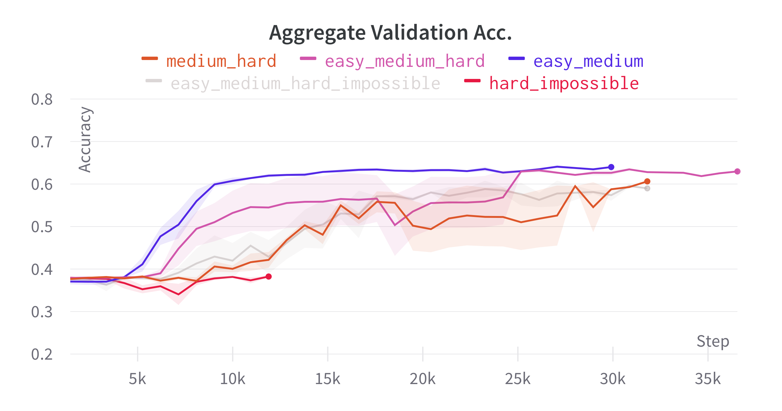
Figure 5: Aggregate validation accuracy for models trained on data of various difficulties. Training data difficulty appears to affect convergence speed: models trained on easier training sets converge earlier, whilst inclusion of hard and impossible models requires more steps to converge. In our experiments, models trained only on hard/impossible examples never surpass at-chance performance and suffer from model failure more often.

Acquisition Factor

For the multi-source experiments we also plot the acquisition factors: a source-strategy-specific statistic which indicates how much data of a given source is acquired by some strategy, normalized by the share of that source in the unlabelled pool at the time of that acquisition round. This statistic is useful to interpret how much a strategy tends to acquisition of one source relative to others.

We normalize to correct for the effect that acquiring e.g. mostly SNLI data in an early round causes it to take up a relatively smaller share in the unlabelled pool in the next round, and by the simple consequence of there being fewer SNLI examples, they may have a lower likelihood to be acquired in those future rounds compared to examples from other sources.. As this could distort our impressions of the extent to which strategies acquire examples from different sources, we ideally want to correct for this.

We thus compute the acquisition factor for a given round as (1) the amount of source examples that were actually acquired by the strategy for that round, divided by (2) the amount of source examples that would be acquired under random sampling from the unlabelled pool at that point. For instance, if BALD has an acquisition factor of $>1$ for SNLI, it means that it acquired more SNLI examples from the unlabeled pool than it would have under random sampling. Conversely, the Random sampling baseline will always have consistent acquisition factors of 1, since the quantities in the numerator and denominator will be approximately the same: random selection always acquire as much from a source as it would under random selection. See Figure 6 for a graphical explanation.

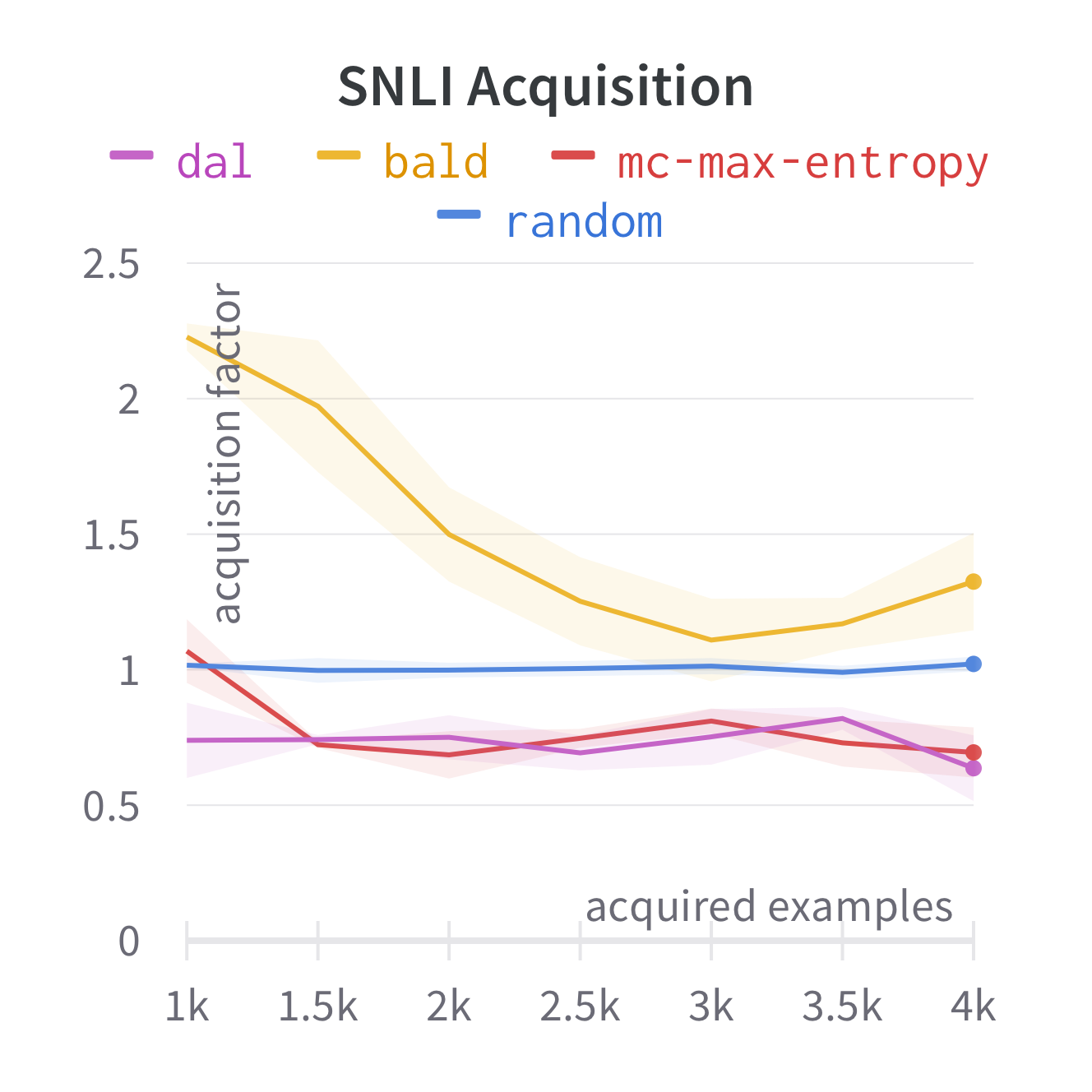
(a) SNLI Acquisition factors

(b) Acquisitions by source

(c) Acquisitions by source

Figure 6: Acquisition factor explained. By design, random selection acquires a random sample of the unlabelled pool. Since the pool is initialized with even amounts of each source, random consistently acquires a uniform sample over sources, as can be seen in (b). Consequently, the SNLI acquisition factor for Random steadily hovers around 1 in (a). Conversely, BALD initially acquires mostly SNLI examples, as reflected by its high initial acquisition factor. This corresponds to its absolute acquisition statistics in (c), where we note that initially BALD acquires predominantly SNLI.

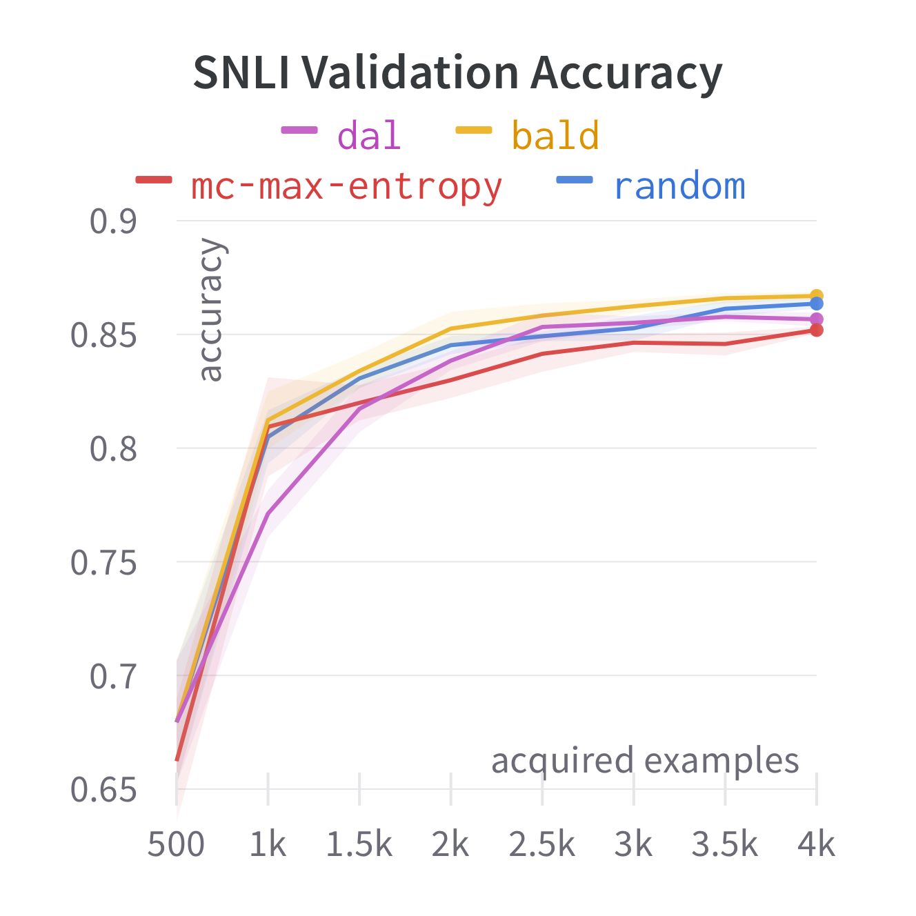
(a) SNLI Val. Acc.

(b) SNLI Acquisition

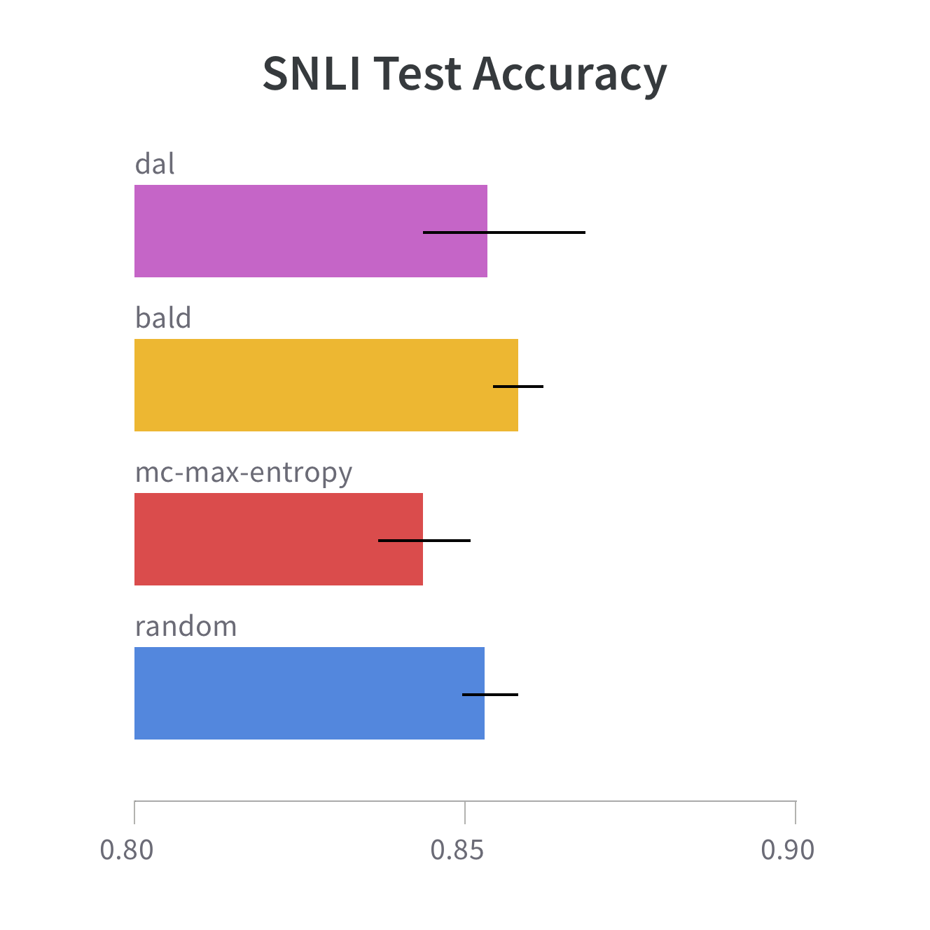
(c) SNLI Test Acc.

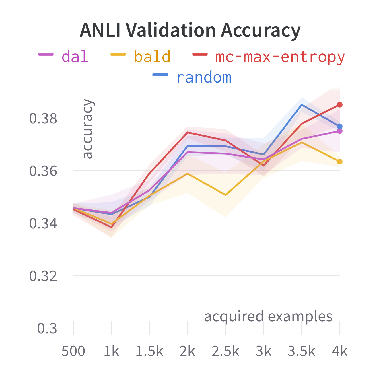
(d) ANLI Val. Acc.

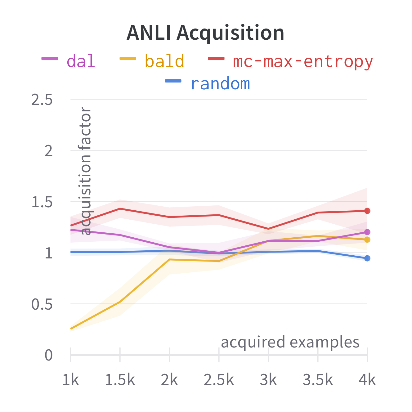
(e) ANLI Acquisition

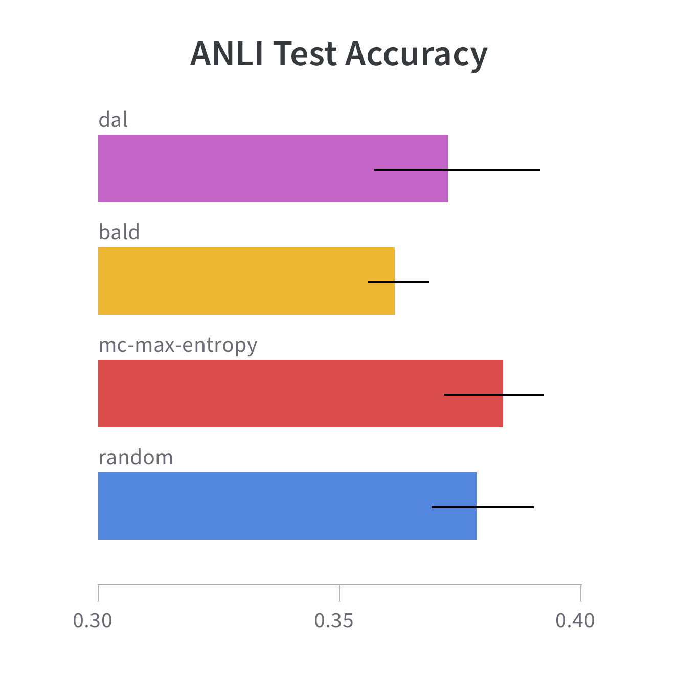
(f) ANLI Test Acc.

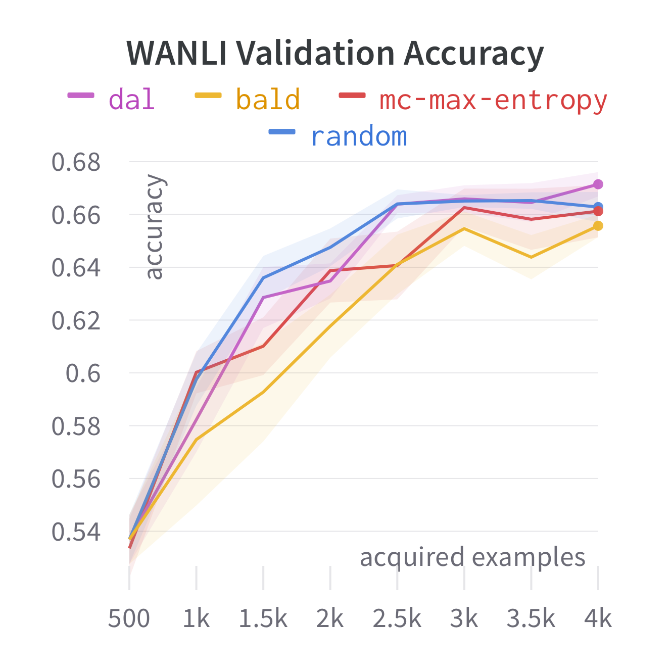
(g) WANLI Val. Acc.

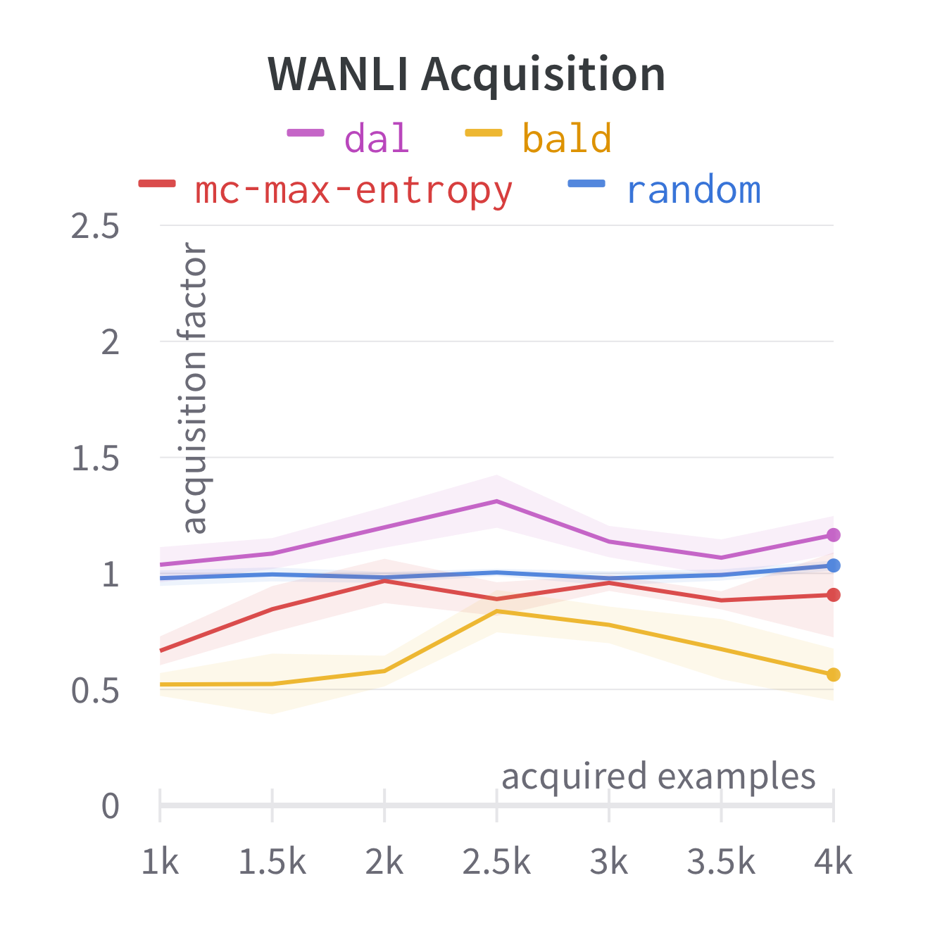
(h) WANLI Acquisition

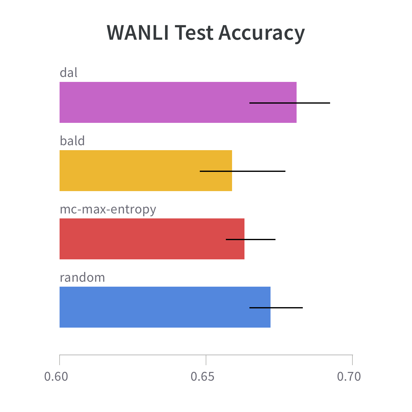
(i) WANLI Test Acc.

Figure 7: In-domain multi-source Active Learning. The left-most graph represents the learning curve per strategy, plotting the validation performance as more labelled data is acquired. The middle graph plots the acquisition factor per source: how much a strategy acquires of a source, normalized by the share that source takes up in the wider data pool. Shaded regions indicate standard errors. Active learning fails to consistently beat random.

9.5 Dataset Cartography

As mentioned in Section 6.1, we train a RoBERTa-large model on a training set comprised of the entire unlabelled pool of training examples, i.e. $60$K examples in total. Every $\frac{1}{2}$ epoch we perform inference on the full training set to get per-example confidence statistics, where the prediction logit corresponding to the gold-truth label serves as a proxy for model confidence. Variability is computed as the standard deviation over the set of confidence measurements. We stop training after $3$ epochs or after no improvement in validation accuracy on the aggregate of validation sets was observed. Following Karamcheti et al. (2021), we classify examples along four difficulties via a threshold on the mean confidence value $p$.

Note on model discrepancy

When studying the strategy maps, it is instructive to note that there exists a discrepancy between models which may distort the truthfulness of learnability measurements. That is, the cartography model that was used to obtain confidence/variability measurements for datamap construction was trained on the entire pool of 60K examples, whereas the model used during AL is exposed to at most 4K examples after completing all rounds of acquisition. Consequently, examples which were found to be easy by the cartography model are likely to be substantially more difficult for the AL model. As datamaps are inherently model-based, the generated strategy maps should be interpreted as skewed estimates of the true learnability spectra. While we recognize the potential value of preserving scale equivalence when using dataset cartography for analysis, we choose to follow Karamcheti et al. (2021) and intend to employ datamaps as a post-hoc diagnostic tool. In other words, we are interested in examining example learnability in an absolute sense (i.e. with respect to the entire pool) rather than a relative sense (with respect to the acquired data). Here, we also note that a model trained on a larger set of examples will likely more accurately reflect the true difficulty of examples. This is important if we want to draw new insights on the learnability of NLI datasets in a wider sense.

Task	Diff.	Random	MCME	BALD	DAL
	E	$95.4\pm 0.9\mid 95.0\pm 0.4$	$95.0\pm 0.5\mid 93.3\pm 0.7$	$95.5\pm 1.0\mid 94.8\pm 0.3$	$93.7\pm 1.2\mid 94.6\pm 0.8$
SNLI	M	$69.0\pm 2.6\mid 67.7\pm 1.2$	$70.2\pm 1.6\mid 68.0\pm 1.2$	$70.5\pm 2.6\mid 69.5\pm 1.2$	$67.8\pm 2.4\mid 68.2\pm 2.5$
	H	$46.3\pm 3.5\mid 44.6\pm 1.9$	$48.5\pm 1.6\mid 46.0\pm 2.2$	$47.1\pm 3.2\mid 49.2\pm 2.9$	$44.7\pm 2.2\mid 45.8\pm 3.9$
	I	$17.7\pm 1.7\mid 17.2\pm 1.7$	$20.3\pm 2.4\mid 22.1\pm 0.9$	$20.7\pm 1.7\mid 22.2\pm 0.4$	$18.4\pm 2.0\mid 17.5\pm 2.2$
	E	$81.4\pm 4.9\mid 81.7\pm 4.3$	$77.0\pm 4.1\mid 79.2\pm 1.4$	$82.1\pm 3.1\mid 73.8\pm 2.1$	$81.8\pm 3.5\mid 79.9\pm 3.4$
ANLI	M	$62.2\pm 2.7\mid 62.1\pm 0.4$	$61.7\pm 3.5\mid 57.8\pm 0.9$	$61.1\pm 1.6\mid 57.1\pm 4.0$	$63.1\pm 2.3\mid 59.8\pm 3.1$
	H	$39.3\pm 3.3\mid 40.2\pm 0.7$	$42.9\pm 3.2\mid 41.6\pm 2.4$	$39.2\pm 2.6\mid 39.7\pm 2.6$	$39.0\pm 2.0\mid 38.5\pm 1.5$
	I	$14.4\pm 2.4\mid 14.2\pm 2.2$	$15.7\pm 2.0\mid 17.0\pm 0.8$	$12.6\pm 1.2\mid 14.5\pm 1.8$	$14.2\pm 1.7\mid 15.0\pm 1.9$
	E	$94.3\pm 2.0\mid 92.9\pm 1.4$	$92.7\pm 0.8\mid 91.2\pm 0.7$	$95.2\pm 0.9\mid 90.9\pm 1.1$	$94.1\pm 0.4\mid 93.1\pm 1.3$
WANLI	M	$72.7\pm 3.2\mid 69.6\pm 3.5$	$71.4\pm 1.2\mid 69.9\pm 2.2$	$72.7\pm 1.7\mid 67.9\pm 3.0$	$72.3\pm 3.1\mid 73.8\pm 2.1$
	H	$41.9\pm 2.7\mid 40.4\pm 1.6$	$43.1\pm 2.6\mid 44.2\pm 1.2$	$42.4\pm 4.6\mid 40.7\pm 2.6$	$40.6\pm 1.9\mid 41.0\pm 3.4$
	I	$12.7\pm 1.5\mid 14.4\pm 1.4$	$14.0\pm 2.0\mid 16.6\pm 4.7$	$11.9\pm 2.6\mid 14.7\pm 4.4$	$13.9\pm 2.8\mid 14.6\pm 3.6$
	E	$93.3\pm 2.0\mid 93.6\pm 0.6$	$94.3\pm 0.9\mid 92.8\pm 1.2$	$94.4\pm 0.8\mid 92.4\pm 0.8$	$93.4\pm 1.3\mid 93.8\pm 1.5$
MNLI	M	$72.6\pm 3.8\mid 72.9\pm 1.5$	$78.6\pm 2.0\mid 74.7\pm 4.6$	$75.9\pm 1.6\mid 72.8\pm 4.4$	$74.7\pm 3.4\mid 78.1\pm 4.6$
	H	$41.8\pm 3.8\mid 44.5\pm 1.0$	$51.9\pm 4.9\mid 49.3\pm 3.3$	$45.7\pm 4.1\mid 46.7\pm 3.3$	$46.1\pm 3.9\mid 48.3\pm 4.7$
	I	$12.8\pm 3.8\mid 15.7\pm 1.8$	$20.9\pm 2.9\mid 19.5\pm 1.4$	$13.1\pm 2.0\mid 16.9\pm 1.9$	$12.6\pm 2.2\mid 18.5\pm 6.3$
	E	$91.0\pm 6.7\mid 90.8\pm 5.8$	$89.8\pm 7.7\mid 89.1\pm 5.9$	$91.8\pm 5.9\mid 88.0\pm 8.4$	$90.7\pm 5.5\mid 90.4\pm 6.4$
All	M	$69.3\pm 5.3\mid 68.1\pm 4.4$	$70.5\pm 6.4\mid 67.6\pm 6.7$	$70.0\pm 5.8\mid 66.8\pm 6.8$	$69.4\pm 5.2\mid 69.9\pm 7.6$
	H	$42.3\pm 4.2\mid 42.4\pm 2.5$	$46.5\pm 5.1\mid 45.3\pm 3.7$	$43.6\pm 4.8\mid 44.1\pm 4.9$	$42.6\pm 3.9\mid 43.4\pm 5.3$
	I	$14.4\pm 3.3\mid 15.3\pm 2.2$	$17.7\pm 3.8\mid 18.8\pm 3.4$	$14.6\pm 4.1\mid 17.1\pm 4.1$	$14.8\pm 3.2\mid 16.4\pm 4.2$

Table 10: Multi-source in-domain strategy comparison for difficulty-stratified test outcomes between original training set and training set with hard-to-learn examples excluded. Values denote test accuracies and standard deviations. We consider performance on test examples belonging to the Easy (E), Medium (M), Hard (H) and Impossible (I) sets.
Cell scheme to be read as ablated $\mid$ original.

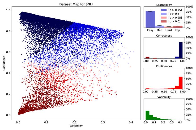
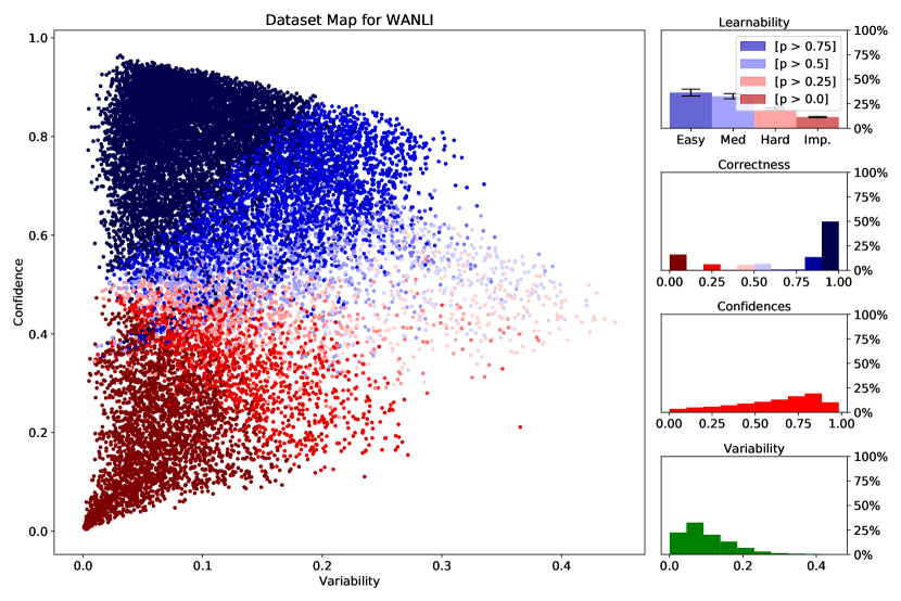
Figure 8: Dataset Maps for SNLI and WANLI training data. The majority of SNLI examples lie in the easy-to-learn region. For WANLI, datapoints are more evenly distributed across the learnability spectrum and exhibit greater variability.

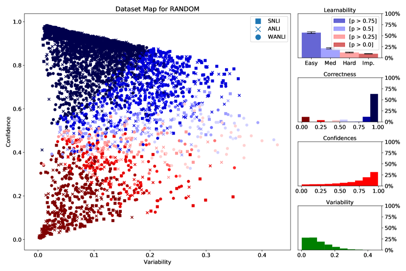
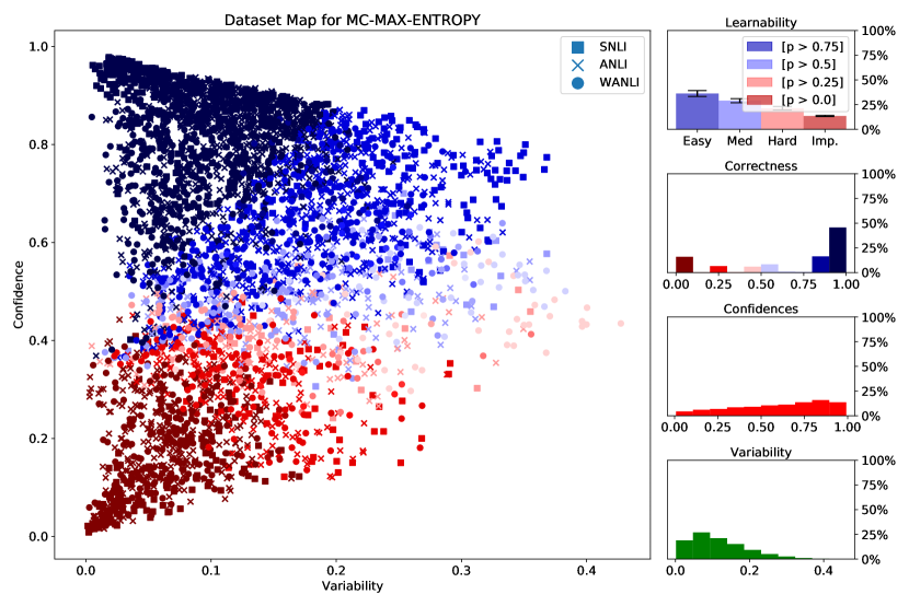
Figure 9: Strategy maps for the Random and MC-Max-entropy strategies for multi-source active learning. The latter acquires considerably more hard-to-learn instances.

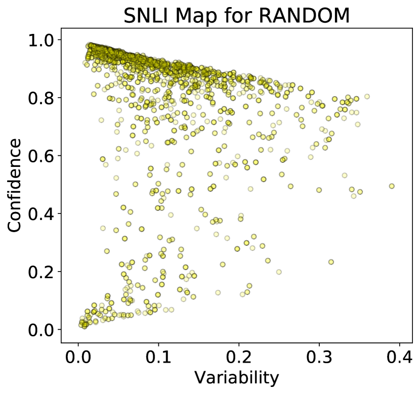
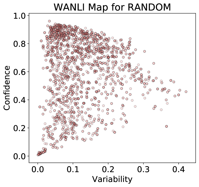
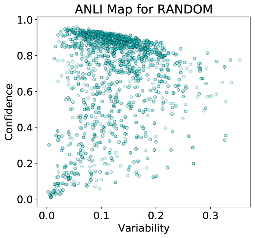
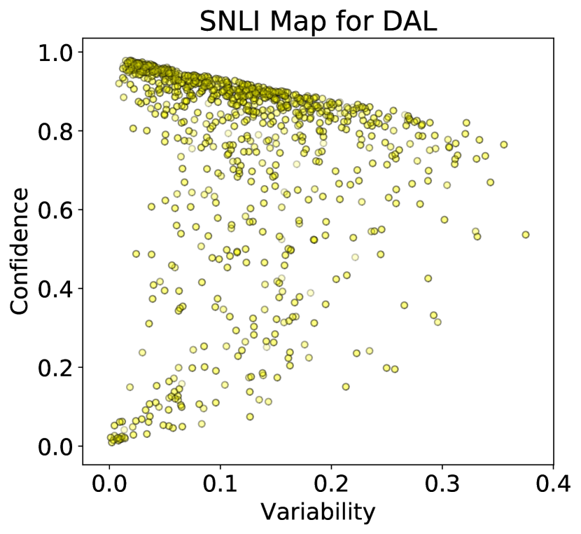
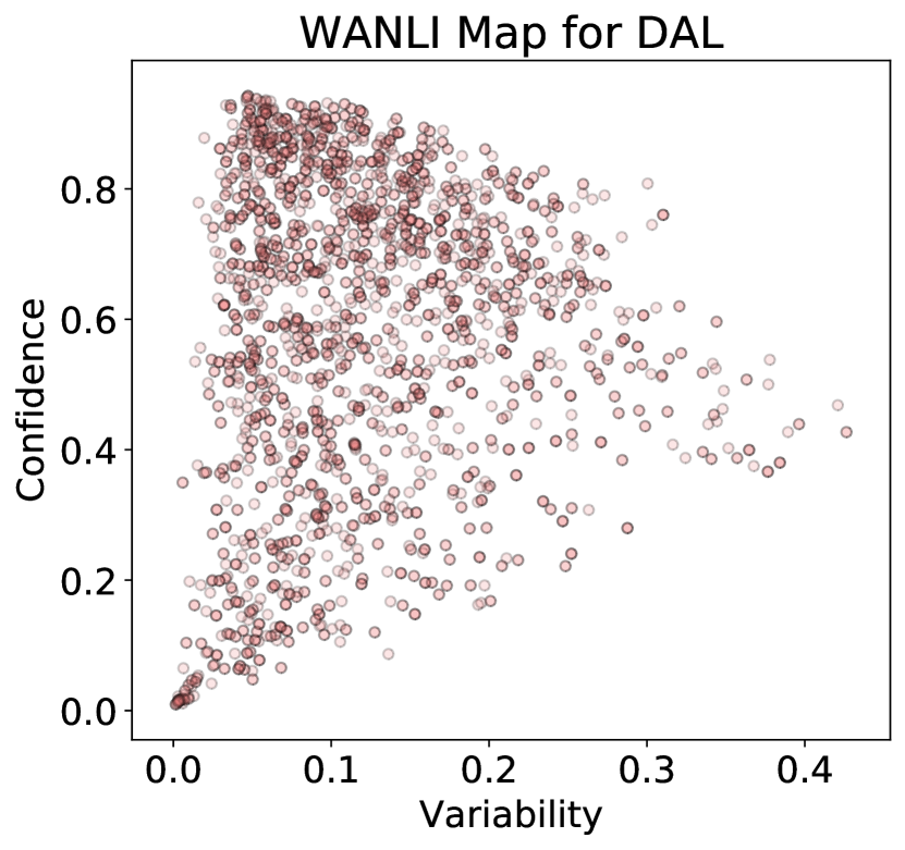
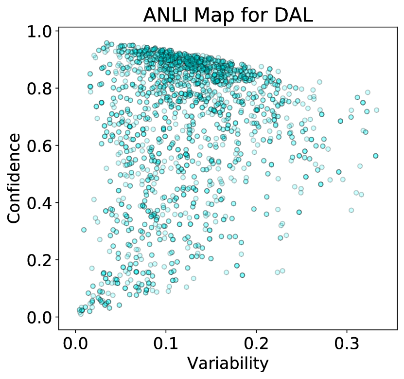
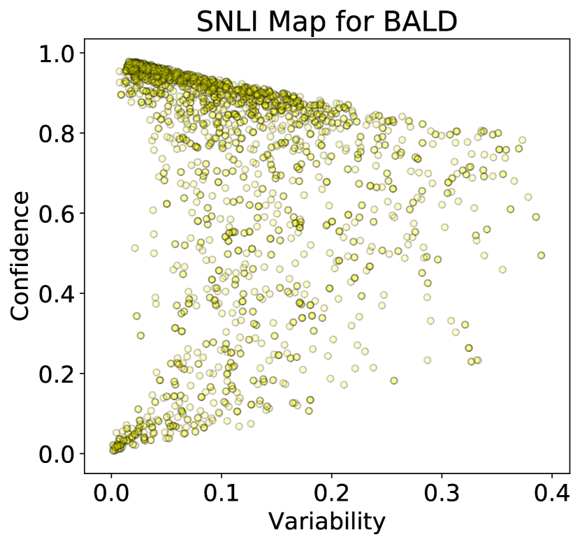
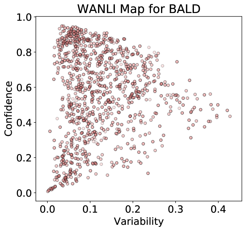
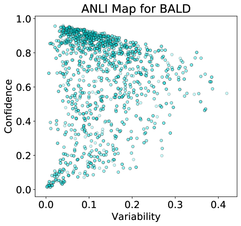
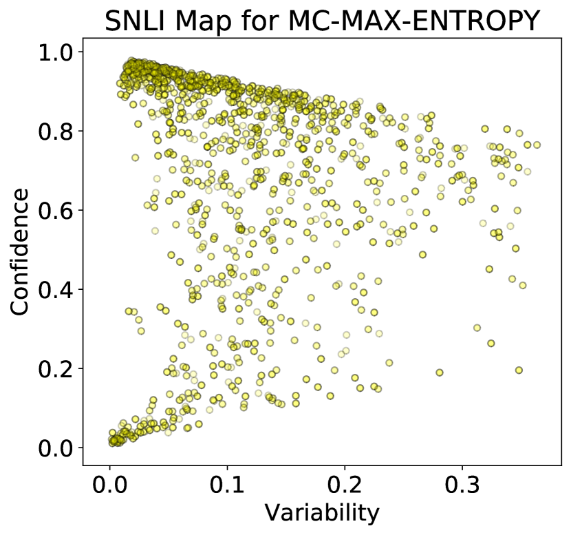
(a) Strategy maps for snli

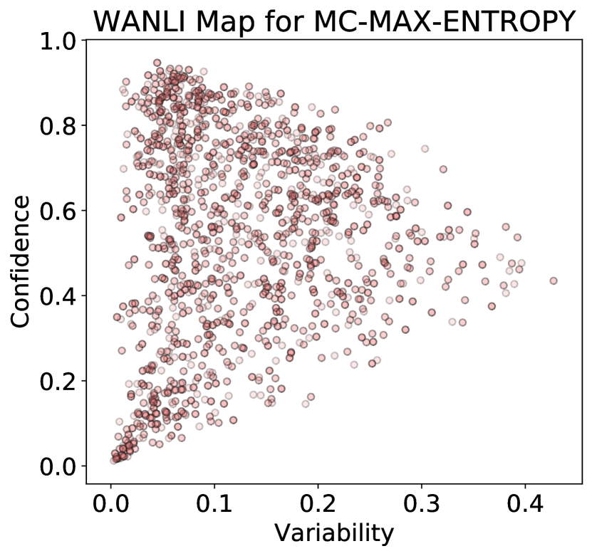
(b) Strategy maps for wanli

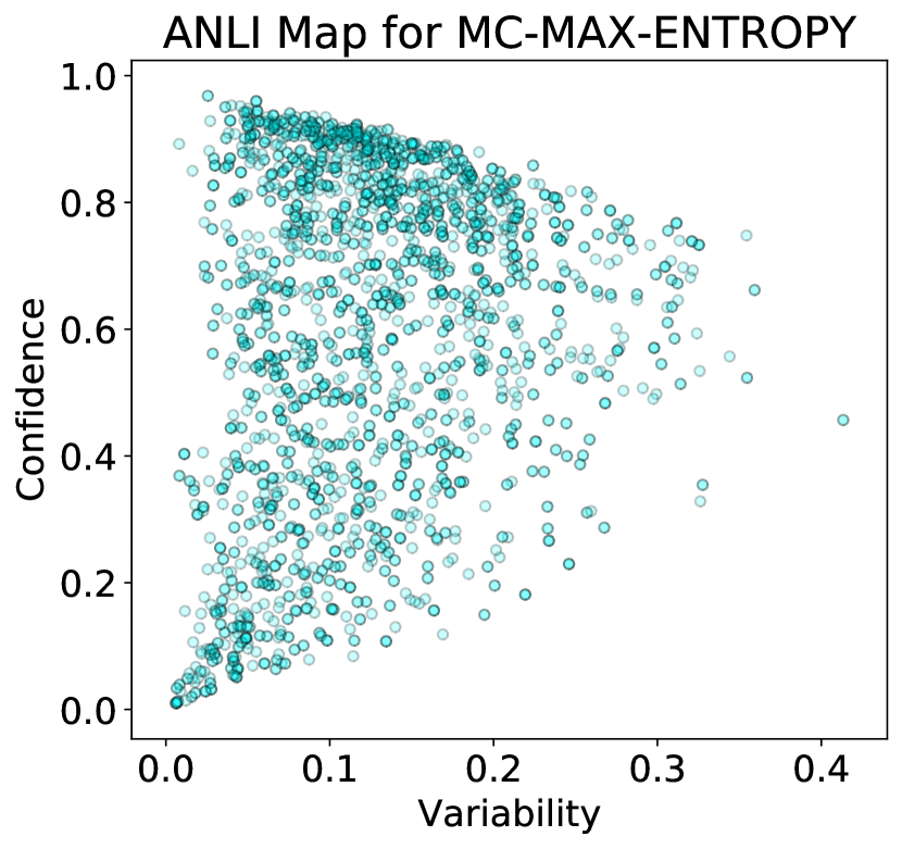
(c) Strategy maps for anli

Figure 10: Strategy maps for multi-source active learning, plotted per source.

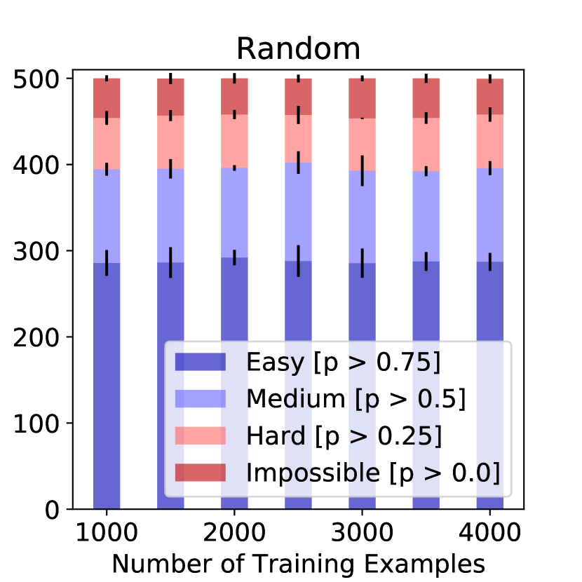
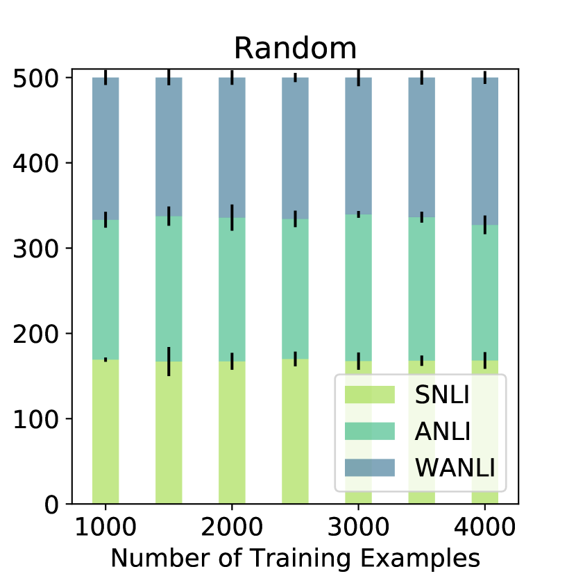
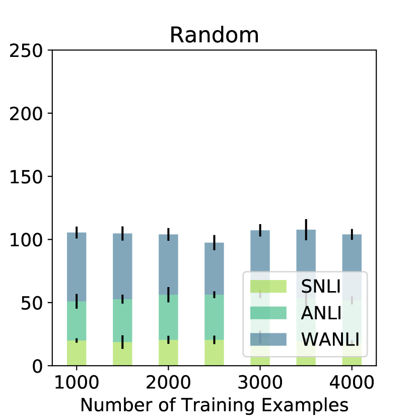
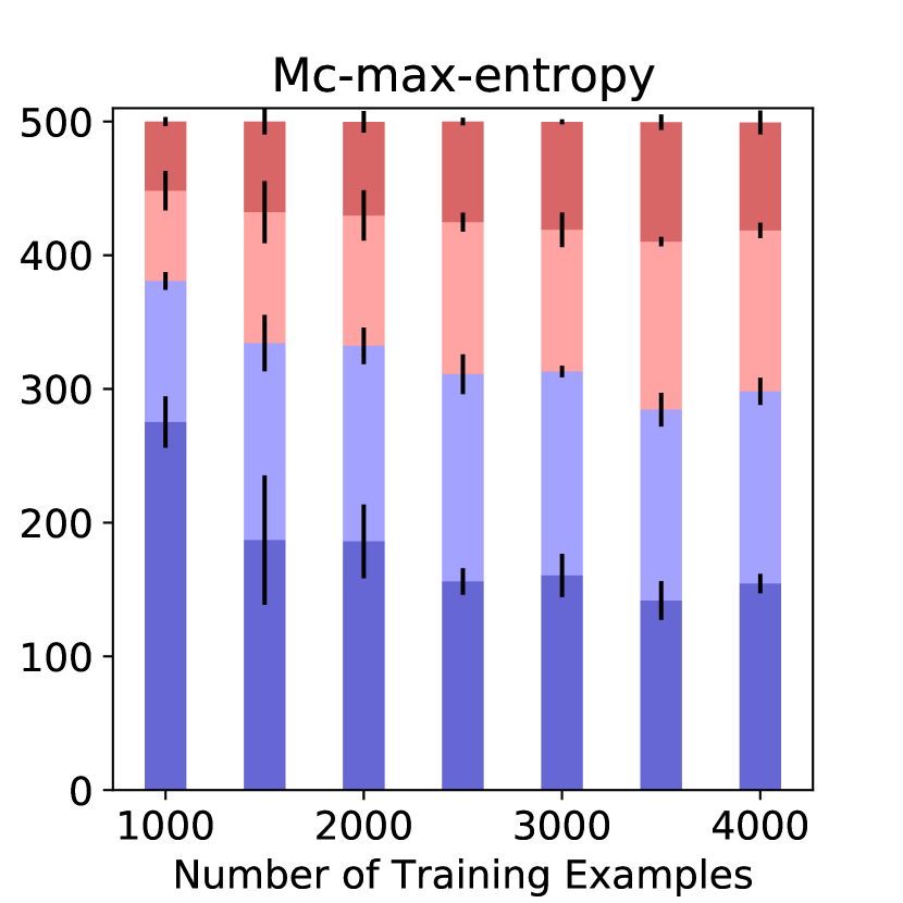
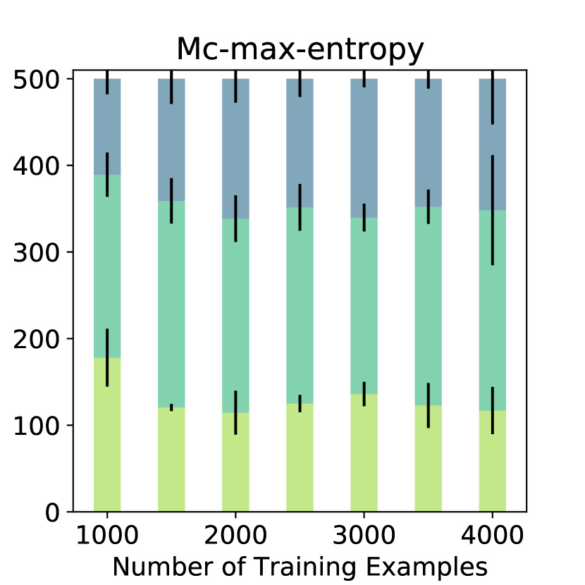
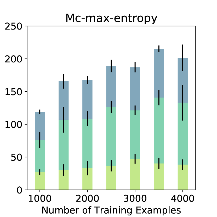
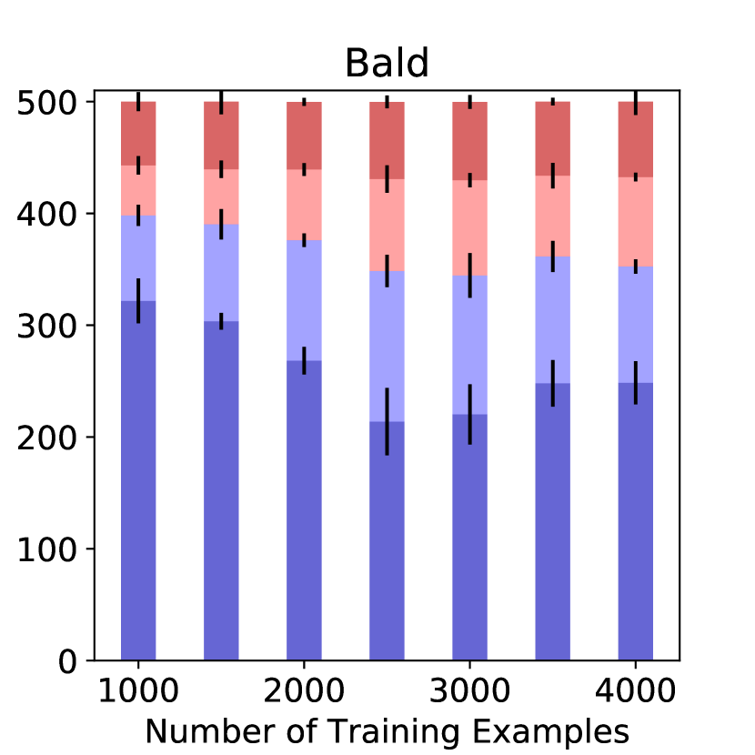
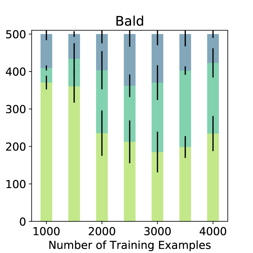
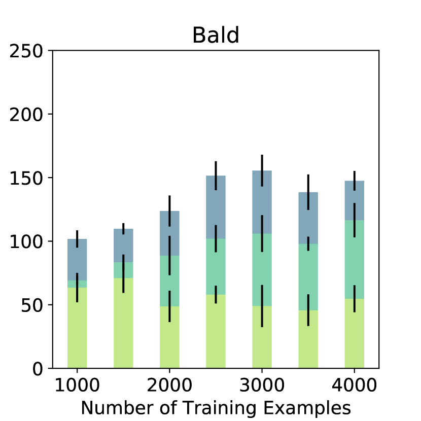
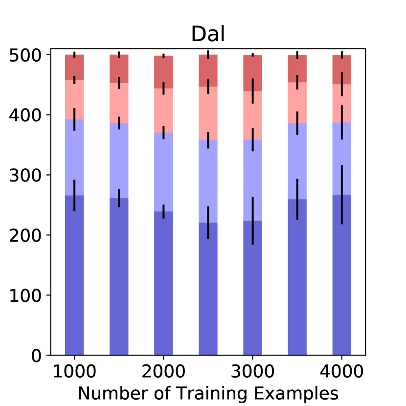
(a) Acquisition by learnability

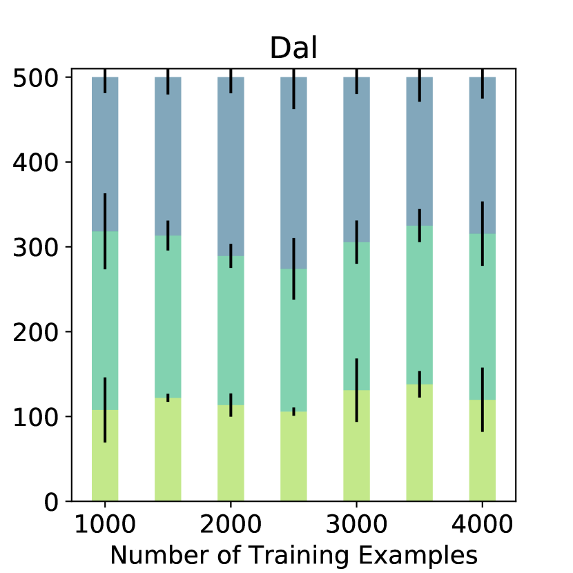
(b) Acquisition per source

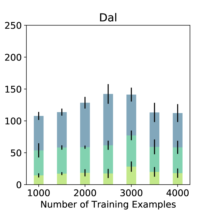
(c) Hard & Imp. per source

Figure 11: Profiling acquisitions for strategies over time. Y-axis denotes amount of acquired examples per round. The right graph plots the acquisition of hard and impossible examples. Dark bars indicate standard deviations across seeds. MCM-Entropy and BALD acquire notably more hard and impossible instances relative to random sampling.

9.6 Impact of data difficulty on training time

We find that models quickly learn simple examples while requiring more iterations for complex ones (See Figure 5). A similar outcome was observed by Lalor et al. (2018) who employ item response theory for data difficulty estimation - interestingly however, their difficulty parameters are estimated via a human population, while our difficulty estimations follow directly from training dynamics. This echoes a similar finding by (Zhang and Plank, 2021), who show that cartography-based model confidence scores strongly correlate with human agreement on SNLI validation data. Similarly, it may be of interest to see whether examples which many different models identify as ambiguous correlate with human judgements of ambiguity, e.g. with respect to human label distributions (Nie et al., 2020; Chen et al., 2020), or annotator disagreement scores.

9.7 Hard-to-learn Data

In the tables below, we present various cases of hard-to-learn examples (i.e., collective outliers) for the NLI datasets we examine.

Table 11: Impossible ($0\leq p\leq 0.25$) training examples from snli. GT denotes the gold truth; P. denotes the model prediction and Conf. the confidence associated with the predicted label.

Ex.	Premise	Hypothesis	GT	P.	Conf.
(1)	A skier in electric green on the edge of a ramp made of metal bars.	The skier was on the edge of the ramp.	N	E	0.976
($2$)	A skier in electric green on the edge of a ramp made of metal bars.	The brightly dressed skier slid down the race course.	E	C	0.770
($3$)	A man wearing a red sweater is sitting on a car bumper watching another person work.	people make speed fast at speed breaker.	C	N	0.799
(4)	Middle-aged female wearing a white sunhat and white jacket, slips her hand inside a man’s pants pocket.	The man and woman are playing together.	C	N	0.869
(5)	A young girl jumps off of a couch and high into the air	the young lady knows how to fly in sky	C	N	0.765
(6)	A young boy jumps into the oncoming wave.	The boy is at a lake.	C	N	0.951
(7)	A woman taking her wallet out of her purse at a vendor stand	A woman buying something from a vendor.	E	N	0.892
(8)	A group of people standing on a rock path.	A group of people are hiking.	E	N	0.972
(9)	Woman sitting in tree with dove.	The lady is touching a dove.	N	E	0.920
(10)	A lady standing on the corner using her phone.	The lady has a smartphone.	N	E	0.753

Table 12: Impossible ($0\leq p\leq 0.25$) training examples from wanli. GT denotes the gold truth; P. denotes the model prediction and Conf. the confidence associated with the predicted label.

Ex.	Premise	Hypothesis	GT	P.	Conf.
(1)	The first principle of art is that art is not a way of life, but a means of life.	Art is a way of life.	E	C	0.944
(2)	"Must be right good stock," Fenner observed.	"Must be pretty good stock," Fenner said.	C	E	0.646
(3)	He believes that the best thing to do is to buy the firm at a reasonable price.	If the firm is cheap, it is best to buy it.	N	E	0.964
(4)	A piece of paper with a stamp on it is worth less than a piece of paper without a stamp.	A piece of paper without a stamp is worth more than a piece of paper with a stamp.	E	C	0.818
(5)	It was the only time he had seen her laugh.	He had never seen her laugh before.	C	N	0.502
(6)	The musician shook his head.	The musician moved his head up and down.	C	E	0.510
(7)	Some students believe that to achieve their goals they must take the lead.	Some students believe that to achieve their goals they must follow the lead.	E	C	0.630
(8)	The very nature of the "American Dream" is that it is not always attainable	The American Dream is attainable.	N	C	0.817
(9)	This might be an issue for a company that is in the process of introducing a new product.	Every company is always in the process of introducing a new product.	E	N	0.894
(10)	Would Higher Interest Rates Stimulate Saving?	Higher interest rates would not stimulate saving.	E	N	0.929

Table 13: Impossible ($0\leq p\leq 0.25$) training examples from anli. GT denotes the gold truth; P. denotes the model prediction and Conf. the confidence associated with the predicted label. Instances are comparatively less characterized by noisy labels or ambiguity; rather, their difficulty arises through requirement of more advanced inference types, e.g. identifying relevant information from long passages, multi-hop reasoning to connect subjects to events and numerical reasoning about dates of birth and events.

Ex.	Premise	Hypothesis	GT	P.	Conf.
(1)	Glaiza Herradura-Agullo (born February 24, 1978) is a Filipino former child actress. She was the first-ever grand winner of the Little Miss Philippines segment of "Eat Bulaga!" in 1984. She starred in RPN-9’s television series "Heredero" with Manilyn Reynes and Richard Arellano. She won the 1988 FAMAS Best Child Actress award for her role in "Batas Sa Aking Kamay" starring Fernando Poe, Jr. .	Herradura-Agullo was born in the 80’s	C	E	0.941
(2)	The Whitechapel murders were committed in or near the impoverished Whitechapel district in the East End of London between 3 April 1888 and 13 February 1891. At various points some or all of these eleven unsolved murders of women have been ascribed to the notorious unidentified serial killer known as Jack the Ripper.	The women killed in the Whitechapel murders were impoverished.	N	E	0.832
(3)	Departure of a Grand Old Man is a 1912 Russian silent film about the last days of author Leo Tolstoy. The film was directed by Yakov Protazanov and Elizaveta Thiman, and was actress Olga Petrova’s first film.	Olga performed in many films before This one	C	N	0.922
(4)	Gay Sex in the 70s is a 2005 American documentary film about gay sexual culture in New York City in the 1970s. The film was directed by Joseph Lovett and encompasses the twelve years of sexual freedom bookended by the Stonewall riots of 1969 and the recognition of AIDS in 1981, and features interviews with Larry Kramer, Tom Bianchi, Barton Lidice Beneš, Rodger McFarlane, and many others.	Gay Sex in the 70s was directed by a gay man.	N	E	0.907
(5)	Héctor Canziani was an Argentine poet, screenwriter and film director who worked in Argentine cinema in the 1940s and 1950s. Although his work was most abundant in screenwriting and poetry after his brief film career, he is best known for his directorship and production of the 1950 tango dancing film Al Compás de tu Mentira based on a play by Oscar Wilde.	He did direct a movie after 1950	N	E	0.944

References

- Bowman et al. (2015) Samuel R Bowman, Gabor Angeli, Christopher Potts, and Christopher D Manning. 2015. A large annotated corpus for learning natural language inference. In Conference Proceedings - EMNLP 2015: Conference on Empirical Methods in Natural Language Processing, pages 632–642.
- Chaudhary et al. (2021) Aditi Chaudhary, Antonios Anastasopoulos, Zaid Sheikh, and Graham Neubig. 2021. Reducing confusion in active learning for part-of-speech tagging. Transactions of the Association for Computational Linguistics, 9:1–16.
- Chen et al. (2020) Tongfei Chen, Zhengping Jiang, Adam Poliak, Keisuke Sakaguchi, and Benjamin Van Durme. 2020. Uncertain natural language inference. In Proceedings of the 58th Annual Meeting of the Association for Computational Linguistics, pages 8772–8779, Online. Association for Computational Linguistics.
- Cohn et al. (1996) David A. Cohn, Zoubin Ghahramani, and Michael I. Jordan. 1996. Active learning with statistical models. Journal of Artificial Intelligence Research, 4(1):129–145.
- Ein-Dor et al. (2020) Liat Ein-Dor, Alon Halfon, Ariel Gera, Eyal Shnarch, Lena Dankin, Leshem Choshen, Marina Danilevsky, Ranit Aharonov, Yoav Katz, and Noam Slonim. 2020. Active learning for BERT: An empirical study. In EMNLP 2020 - 2020 Conference on Empirical Methods in Natural Language Processing, Proceedings of the Conference, pages 7949–7962.
- Gal and Ghahramani (2015) Yarin Gal and Zoubin Ghahramani. 2015. Dropout as a Bayesian Approximation: Representing Model Uncertainty in Deep Learning. 33rd International Conference on Machine Learning, ICML 2016, 3:1651–1660.
- Gal et al. (2017) Yarin Gal, Riashat Islam, and Zoubin Ghahramani. 2017. Deep Bayesian Active Learning with Image Data. 34th International Conference on Machine Learning, ICML 2017, 3:1923–1932.
- Geva et al. (2019) Mor Geva, Yoav Goldberg, and Jonathan Berant. 2019. Are We Modeling the Task or the Annotator? An Investigation of Annotator Bias in Natural Language Understanding Datasets. EMNLP-IJCNLP 2019 - 2019 Conference on Empirical Methods in Natural Language Processing and 9th International Joint Conference on Natural Language Processing, Proceedings of the Conference, pages 1161–1166.
- Ghorbani et al. (2021) Amirata Ghorbani, James Zou, and Andre Esteva. 2021. Data Shapley Valuation for Efficient Batch Active Learning. arXiv preprint 2104.08312.
- Gissin and Shalev-Shwartz (2019) Daniel Gissin and Shai Shalev-Shwartz. 2019. Discriminative Active Learning.
- Gururangan et al. (2018) Suchin Gururangan, Swabha Swayamdipta, Omer Levy, Roy Schwartz, Samuel R. Bowman, and Noah A. Smith. 2018. Annotation Artifacts in Natural Language Inference Data. NAACL HLT 2018 - 2018 Conference of the North American Chapter of the Association for Computational Linguistics: Human Language Technologies - Proceedings of the Conference, 2:107–112.
- Han and Kamber (2000) Jiawei Han and Micheline Kamber. 2000. Data Mining: Concepts and Techniques. Morgan Kaufmann.
- He et al. (2021) Rui He, Shengcai Liu, Shan He, and Ke Tang. 2021. Multi-Domain Active Learning: A Comparative Study. arXiv preprint 2106.13516.
- Houlsby et al. (2011) Neil Houlsby, Ferenc Huszár, Zoubin Ghahramani, and Máté Lengyel. 2011. Bayesian Active Learning for Classification and Preference Learning. CoRR abs/1112.5745.
- Huang et al. (2016) Jiaji Huang, Rewon Child, Vinay Rao, Hairong Liu, Sanjeev Satheesh, and Adam Coates. 2016. Active Learning for Speech Recognition: the Power of Gradients. arXiv preprint arXiv:1612.03226. Published as a workshop paper at NIPS 2016.
- Hupkes et al. (2022) Dieuwke Hupkes, Mario Giulianelli, Verna Dankers, Mikel Artetxe, Yanai Elazar, Tiago Pimentel, Christos Christodoulopoulos, Karim Lasri, Naomi Saphra, Arabella Sinclair, Dennis Ulmer, Florian Schottmann, Khuyagbaatar Batsuren, Kaiser Sun, Koustuv Sinha, Leila Khalatbari, Maria Ryskina, Rita Frieske, Ryan Cotterell, and Zhijing Jin. 2022. State-of-the-art generalisation research in nlp: A taxonomy and review.
- Karamcheti et al. (2021) Siddharth Karamcheti, Ranjay Krishna, Li Fei-Fei, and Christopher D. Manning. 2021. Mind Your Outliers! Investigating the Negative Impact of Outliers on Active Learning for Visual Question Answering. pages 7265–7281.
- Kees et al. (2021) Nataliia Kees, Michael Fromm, Evgeniy Faerman, and Thomas Seidl. 2021. Active learning for argument strength estimation. In Proceedings of the Second Workshop on Insights from Negative Results in NLP, pages 144–150, Online and Punta Cana, Dominican Republic. Association for Computational Linguistics.
- Kirk et al. (2022) Hannah Kirk, Bertie Vidgen, and Scott Hale. 2022. Is more data better? re-thinking the importance of efficiency in abusive language detection with transformers-based active learning. In Proceedings of the Third Workshop on Threat, Aggression and Cyberbullying (TRAC 2022), pages 52–61, Gyeongju, Republic of Korea. Association for Computational Linguistics.
- Kirsch and Gal (2021) Andreas Kirsch and Yarin Gal. 2021. Powerevaluationbald: Efficient evaluation-oriented deep (bayesian) active learning with stochastic acquisition functions. CoRR, abs/2101.03552.
- Kirsch et al. (2021) Andreas Kirsch, Tom Rainforth, and Yarin Gal. 2021. Test Distribution-Aware Active Learning: A Principled Approach Against Distribution Shift and Outliers. arXiv preprint 2106.11719.
- Kreutzer et al. (2022) Julia Kreutzer, Isaac Caswell, Lisa Wang, Ahsan Wahab, Daan van Esch, Nasanbayar Ulzii-Orshikh, Allahsera Tapo, Nishant Subramani, Artem Sokolov, Claytone Sikasote, Monang Setyawan, Supheakmungkol Sarin, Sokhar Samb, Benoît Sagot, Clara Rivera, Annette Rios, Isabel Papadimitriou, Salomey Osei, Pedro Ortiz Suarez, Iroro Orife, Kelechi Ogueji, Andre Niyongabo Rubungo, Toan Q. Nguyen, Mathias Müller, André Müller, Shamsuddeen Hassan Muhammad, Nanda Muhammad, Ayanda Mnyakeni, Jamshidbek Mirzakhalov, Tapiwanashe Matangira, Colin Leong, Nze Lawson, Sneha Kudugunta, Yacine Jernite, Mathias Jenny, Orhan Firat, Bonaventure F. P. Dossou, Sakhile Dlamini, Nisansa de Silva, Sakine Çabuk Ballı, Stella Biderman, Alessia Battisti, Ahmed Baruwa, Ankur Bapna, Pallavi Baljekar, Israel Abebe Azime, Ayodele Awokoya, Duygu Ataman, Orevaoghene Ahia, Oghenefego Ahia, Sweta Agrawal, and Mofetoluwa Adeyemi. 2022. Quality at a glance: An audit of web-crawled multilingual datasets. Transactions of the Association for Computational Linguistics, 10:50–72.
- Lalor et al. (2018) John P. Lalor, Hao Wu, Tsendsuren Munkhdalai, and Hong Yu. 2018. Understanding deep learning performance through an examination of test set difficulty: A psychometric case study. Proceedings of the 2018 Conference on Empirical Methods in Natural Language Processing, EMNLP 2018, pages 4711–4716.
- Liu et al. (2022) Alisa Liu, Swabha Swayamdipta, Noah A Smith, and Yejin Choi. 2022. WANLI: Worker and AI Collaboration for Natural Language Inference Dataset Creation. arXiv preprint arXiv:2201.05955.
- Liu et al. (2018) Ming Liu, Wray Buntine, and Gholamreza Haffari. 2018. Learning to Actively Learn Neural Machine Translation. CoNLL 2018 - 22nd Conference on Computational Natural Language Learning, Proceedings, pages 334–344.
- Liu et al. (2020) Sheng Liu, Jonathan Niles-Weed, Narges Razavian, and Carlos Fernandez-Granda. 2020. Early-learning regularization prevents memorization of noisy labels. Advances in Neural Information Processing Systems, 2020-December.
- Longpre et al. (2022) Shayne Longpre, Julia Reisler, Edward Greg Huang, Yi Lu, Andrew Frank, Nikhil Ramesh, and Chris DuBois. 2022. Active Learning Over Multiple Domains in Natural Language Tasks. arXiv preprint arXiv:2202.00254.
- Loshchilov and Hutter (2018) Ilya Loshchilov and Frank Hutter. 2018. Fixing weight decay regularization in adam.
- Lowell et al. (2019) David Lowell, Zachary C. Lipton, and Byron C. Wallace. 2019. Practical obstacles to deploying active learning. EMNLP-IJCNLP 2019 - 2019 Conference on Empirical Methods in Natural Language Processing and 9th International Joint Conference on Natural Language Processing, Proceedings of the Conference, pages 21–30.
- Margatina et al. (2022) Katerina Margatina, Loic Barrault, and Nikolaos Aletras. 2022. On the importance of effectively adapting pretrained language models for active learning. In Proceedings of the 60th Annual Meeting of the Association for Computational Linguistics (Volume 2: Short Papers), pages 825–836, Dublin, Ireland. Association for Computational Linguistics.
- Margatina et al. (2021) Katerina Margatina, Giorgos Vernikos, Loïc Barrault, and Nikolaos Aletras. 2021. Active learning by acquiring contrastive examples. In Proceedings of the 2021 Conference on Empirical Methods in Natural Language Processing, pages 650–663, Online and Punta Cana, Dominican Republic. Association for Computational Linguistics.
- Nie et al. (2019) Yixin Nie, Adina Williams, Emily Dinan, Mohit Bansal, Jason Weston, and Douwe Kiela. 2019. Adversarial NLI: A New Benchmark for Natural Language Understanding. pages 4885–4901.
- Nie et al. (2020) Yixin Nie, Xiang Zhou, and Mohit Bansal. 2020. What Can We Learn from Collective Human Opinions on Natural Language Inference Data? EMNLP 2020 - 2020 Conference on Empirical Methods in Natural Language Processing, Proceedings of the Conference, pages 9131–9143.
- Peris and Casacuberta (2018) Álvaro Peris and Francisco Casacuberta. 2018. Active Learning for Interactive Neural Machine Translation of Data Streams. CoNLL 2018 - 22nd Conference on Computational Natural Language Learning, Proceedings, pages 151–160.
- Poliak et al. (2018) Adam Poliak, Jason Naradowsky, Aparajita Haldar, Rachel Rudinger, and Benjamin van Durme. 2018. Hypothesis Only Baselines in Natural Language Inference. NAACL HLT 2018 - Lexical and Computational Semantics, SEM 2018, Proceedings of the 7th Conference, pages 180–191.
- Prabhu et al. (2019) Ameya Prabhu, Charles Dognin, and Maneesh Singh. 2019. Sampling bias in deep active classification: An empirical study. In Proceedings of the 2019 Conference on Empirical Methods in Natural Language Processing and the 9th International Joint Conference on Natural Language Processing (EMNLP-IJCNLP), pages 4058–4068, Hong Kong, China. Association for Computational Linguistics.
- Schröder et al. (2022) Christopher Schröder, Andreas Niekler, and Martin Potthast. 2022. Revisiting uncertainty-based query strategies for active learning with transformers. In Findings of the Association for Computational Linguistics: ACL 2022, pages 2194–2203, Dublin, Ireland. Association for Computational Linguistics.
- Sener and Savarese (2018) Ozan Sener and Silvio Savarese. 2018. Active learning for convolutional neural networks: A core-set approach. 6th International Conference on Learning Representations, ICLR 2018 - Conference Track Proceedings.
- Settles (2010) Burr Settles. 2010. Active Learning Literature Survey. Machine Learning, 15(2):201–221.
- Shelmanov et al. (2021) Artem Shelmanov, Dmitri Puzyrev, Lyubov Kupriyanova, Denis Belyakov, Daniil Larionov, Nikita Khromov, Olga Kozlova, Ekaterina Artemova, Dmitry V. Dylov, and Alexander Panchenko. 2021. Active learning for sequence tagging with deep pre-trained models and Bayesian uncertainty estimates. EACL 2021 - 16th Conference of the European Chapter of the Association for Computational Linguistics, Proceedings of the Conference, pages 1698–1712.
- Shen et al. (2017) Yanyao Shen, Hyokun Yun, Zachary C. Lipton, Yakov Kronrod, and Animashree Anandkumar. 2017. Deep Active Learning for Named Entity Recognition. Proceedings of the 2nd Workshop on Representation Learning for NLP, Rep4NLP 2017 at the 55th Annual Meeting of the Association for Computational Linguistics, ACL 2017, pages 252–256.
- Siddhant and Lipton (2018) Aditya Siddhant and Zachary C. Lipton. 2018. Deep Bayesian Active Learning for Natural Language Processing: Results of a Large-Scale Empirical Study. Proceedings of the 2018 Conference on Empirical Methods in Natural Language Processing, EMNLP 2018, pages 2904–2909.
- Swayamdipta et al. (2020) Swabha Swayamdipta, Roy Schwartz, Nicholas Lourie, Yizhong Wang, Hannaneh Hajishirzi, Noah A. Smith, and Yejin Choi. 2020. Dataset Cartography: Mapping and Diagnosing Datasets with Training Dynamics. EMNLP 2020 - 2020 Conference on Empirical Methods in Natural Language Processing, Proceedings of the Conference, pages 9275–9293.
- Tsuchiya (2018) Masatoshi Tsuchiya. 2018. Performance impact caused by hidden bias of training data for recognizing textual entailment. In Proceedings of the Eleventh International Conference on Language Resources and Evaluation (LREC 2018), Miyazaki, Japan. European Language Resources Association (ELRA).
- Williams et al. (2017) Adina Williams, Nikita Nangia, and Samuel R. Bowman. 2017. A Broad-Coverage Challenge Corpus for Sentence Understanding through Inference. NAACL HLT 2018 - 2018 Conference of the North American Chapter of the Association for Computational Linguistics: Human Language Technologies - Proceedings of the Conference, 1:1112–1122.
- Wolf et al. (2019) Thomas Wolf, Lysandre Debut, Victor Sanh, Julien Chaumond, Clement Delangue, Anthony Moi, Pierric Cistac, Tim Rault, Rémi Louf, Morgan Funtowicz, Joe Davison, Sam Shleifer, Patrick von Platen, Clara Ma, Yacine Jernite, Julien Plu, Canwen Xu, Teven Le Scao, Sylvain Gugger, Mariama Drame, Quentin Lhoest, and Alexander M. Rush. 2019. HuggingFace’s Transformers: State-of-the-art Natural Language Processing. arXiv preprint arXiv:1910.03771.
- Yuan et al. (2020) Michelle Yuan, Hsuan-Tien Lin, and Jordan Boyd-Graber. 2020. Cold-start active learning through self-supervised language modeling. In Proceedings of the 2020 Conference on Empirical Methods in Natural Language Processing (EMNLP), pages 7935–7948, Online. Association for Computational Linguistics.
- Yuan et al. (2022) Michelle Yuan, Patrick Xia, Chandler May, Benjamin Van Durme, and Jordan Boyd-Graber. 2022. Adapting coreference resolution models through active learning. In Proceedings of the 60th Annual Meeting of the Association for Computational Linguistics (Volume 1: Long Papers), pages 7533–7549, Dublin, Ireland. Association for Computational Linguistics.
- Zhang and Plank (2021) Mike Zhang and Barbara Plank. 2021. Cartography Active Learning. Findings of the Association for Computational Linguistics, Findings of ACL: EMNLP 2021, pages 395–406.
- Zhang et al. (2016) Ye Zhang, Matthew Lease, and Byron C. Wallace. 2016. Active Discriminative Text Representation Learning. 31st AAAI Conference on Artificial Intelligence, AAAI 2017, pages 3386–3392.
- Zhang et al. (2022) Zhisong Zhang, Emma Strubell, and Eduard Hovy. 2022. A Survey of Active Learning for Natural Language Processing. EMNLP 2022 - Conference on Empirical Methods in Natural Language Processing, Proceedings.
- Zhao et al. (2020) Yuekai Zhao, Haoran Zhang, Shuchang Zhou, and Zhihua Zhang. 2020. Active Learning Approaches to Enhancing Neural Machine Translation. Findings of the Association for Computational Linguistics Findings of ACL: EMNLP 2020, pages 1796–1806.
- Zhdanov (2019) Fedor Zhdanov. 2019. Diverse mini-batch Active Learning. arXiv preprint 1901.05954v1.