A degenerate Arnold Diffusion Mechanism in the Restricted 3 Body Problem

Abstract.

A major question in dynamical systems is to understand the mechanisms driving global instability in the 3 Body Problem (3BP), which models the motion of three bodies under Newtonian gravitational interaction. The 3BP is called restricted if one of the bodies has zero mass and the other two, the primaries, have strictly positive masses $m_{0},m_{1}$. We consider the Restricted Planar Elliptic 3 Body Problem (RPE3BP) where the primaries revolve in Keplerian ellipses. We prove that the RPE3BP exhibits topological instability: for any values of the masses $m_{0},m_{1}$ (except $m_{0}=m_{1}$), we build orbits along which the angular momentum of the massless body experiences an arbitrarily large variation provided the eccentricity of the orbit of the primaries is positive but small enough.

In order to prove this result we show that a degenerate Arnold Diffusion Mechanism, which moreover involves exponentially small phenomena, takes place in the RPE3BP. Our work extends the result obtained in [DKdlRS19] for the a priori unstable case $m_{1}/m_{0}\ll 1$, to the case of arbitrary masses $m_{0},m_{1}>0$, where the model displays features of the so-called a priori stable setting.

1. Introduction

The $N$ Body Problem models the motion of $N$ bodies under mutual gravitational interaction. Understanding its global dynamics for $N\geq 3$ (the system is integrable for $N=2$) is probably one of the oldest (and more challenging) questions in dynamical systems. A major achievement in this direction was the proof of the existence of a positive measure set of quasiperiodic motions in the $N$ Body Problem. This result was first established by Arnold in [Arn63], who gave a master application of the KAM technique to the case of $3$ coplanar bodies. The proof was later extended to case of $N\geq 3$ in the work of Féjoz and Herman [Fej04] (see also [Rob95, CP11]). On the other hand, in accordance with the general belief that the $N$ Body Problem, although strongly degenerate, displays the main features of a "typical" Hamiltonian system, in his ICM address, Herman conjectured [Her98] that the set of non wandering points for the flow of the $N$ Body Problem is nowhere dense on every energy level for $N\geq 3$. This would imply topological instability for the $N$ Body Problem in a very strong sense.

The existence of topological instability in Hamiltonian systems was first investigated by Arnold in [Arn64], where he constructed an example of nearly integrable Hamiltonian in which this kind of behavior occurs. To that end, Arnold proposed a mechanism giving raise to unstable motions based on the existence of a transition chain of invariant tori: a sequence of invariant irrational tori which are connected by transverse heteroclinic orbits. This mechanism is nowadays called the Arnold mechanism. Arnold verified that this mechanism takes place in a cleverly built model usually referred to as the Arnold model, and he conjectured that topological instability is indeed a common phenomenon in the complement of integrable Hamiltonian Systems [Arn63]. Despite the enormous amount of research (see for example [Dou88, BT99, DdlLS00, MS02, BB02, Mat03, CY04, Tre04, DdlLS06, Ber08, GT08, DH09, NP12, Tre12, BKZ16, DdlLS16, Che17, GT17, KZ20, GdlLS20]) the Arnold diffusion phenomenon, and more generally the dynamics in the complement of the KAM tori set, is still poorly understood (and even more poorly for real analytic or non-convex Hamiltonians).

In [Arn64], Arnold conjectured that the mechanism of instability based on the existence of transition chains “is applicable to the general case (for example, to the problem of 3 bodies)”. However, results concerning the existence of Arnold diffusion in the 3 Body Problem or related models are rather scarce (see [CG18, DKdlRS19, CFG22] and also [DGR16, FGKR16] for numerical based results).

The 3 Body Problem is called “restricted” if one of the bodies has zero mass and the other two, the primaries, have strictly positive masses $m_{0},m_{1}$. In this limit problem, the motion of the primaries is just a 2 Body Problem and the dynamics of the massless body is governed by the gravitational interaction with the primaries. In this work, we consider the case in which the primaries revolve around each other in Keplerian ellipses of eccentricity $\epsilon\in(0,1)$ and the massless body moves on the same plane as the primaries. This model, usually known in the literature as the Restricted Planar Elliptic 3 Body Problem (RPE3BP), is a $2+1/2$ degrees of freedom Hamiltonian system. For $\epsilon=0$ (i.e. for the Restricted Planar Circular 3 Body Problem), the rotational symmetry prevents the existence of topological instability in nearly integrable settings (see Remark 2 below).

The goal of this paper is to prove that a degenerate Arnold Diffusion mechanism takes place in the RPE3BP: we show that for any value of the masses of the primaries ($m_{0}\neq m_{1}$), there exist orbits of the RPE3BP along which the angular momentum of the massless body experiences any predetermined drift provided the eccentricity of the orbits of the primaries is positive but small enough. Notice that the angular momentum is a conserved quantity in the 2 Body Problem, which can be seen as a limit problem of the Restricted 3 Body Problem when $m_{1}/m_{0}\to 0$.

To the best of our knowledge the first complete proof of existence of Arnold Diffusion in Celestial Mechanics was obtained in [DKdlRS19], in which the authors showed the existence of topological instability in the RPE3BP. Nevertheless, this result was established under the strong hypothesis $m_{1}/m_{0}\ll 1$ (see Section 1.2 for a more precise description of the setting). Under this condition, the problem falls in the a priori unstable case for the study of Arnold diffusion and can be analyzed by means of classical perturbation theory. Our result extends the work in [DKdlRS19] to the case of arbitrary masses $m_{0},m_{1}>0$, a setting in which the problem displays many features of the so-called a priori stable case.

1.1. Main Result

Fix a Cartesian reference system with origin at the center of mass of the primaries and choose units so that the total mass of the primaries is equal to $1$. In these coordinates, the primaries, which we denote by $q_{0}$ and $q_{1}$, move along Keplerian ellipses of eccentricity $\epsilon\in(0,1)$ whose time parametrization reads

$$q_{0}(t)=\mu\varrho(t)(\cos f(t),\sin f(t))\qquad\qquad q_{1}(t)=-(1-\mu)\varrho(t)(\cos f(t),\sin f(t)),$$

where $m_{0}=1-\mu$ and $m_{1}=\mu\in(0,1/2]$ are the masses of $q_{0}$ and $q_{1}$, $\varrho(t)$ is the distance between the primaries and is given by

$$\varrho(t)=\frac{1-\epsilon^{2}}{1+\epsilon\cos f(t)}$$

and the so called true anomaly $f(t)$ is determined implicitely by the equation

$$\frac{\mathrm{d}f}{\mathrm{d}t}=\frac{(1+\epsilon\cos f)^{2}}{(1-\epsilon)^{3/2}},\qquad\qquad f(0)=0.$$

The RPE3BP describes the motion of a massless body $q\in\mathbb{R}^{2}$ in the gravitational field generated by the primaries and it is governed by the second order differential equation

(1.1) $$\ddot{q}=(1-\mu)\frac{q-q_{0}(t)}{|q-q_{0}(t)|^{3}}+\mu\frac{q-q_{1}(t)}{|q-q_{1}(t)|^{3}}.$$

It is a classical fact that the RPE3BP admits a Hamiltonian structure. Introducing $p$ and $E$ the conjugate momenta to $q$ and $t$, and the gravitational potential

$$U(q,t)=\frac{1-\mu}{|q-q_{0}(t)|}+\frac{\mu}{|q-q_{1}(t)|}$$

the RPE3BP is Hamiltonian with respect to

$$\mathcal{H}(q,p,t,E)=\frac{|p|^{2}}{2}-U(q,t)+E$$

and the canonical symplectic structure in the extended phase space $T^{*}(\mathbb{R}^{2}\times\mathbb{T})$. The following is our main result.

Theorem 1.1.

Let $G(q,p)=|q\wedge p|$ be the angular momentum of the massless body. Then, for any $\mu\in(0,1/2)$, there exists $G_{*}>0$ such that, for any $\epsilon\in(0,G_{*}^{-3})$ and any values $G_{1},G_{2}$ satisfying

$$G_{*}\leq G_{1}<G_{2}\leq\epsilon^{-1/3},$$

there exists $T>0$ and an orbit $\gamma$ of the RPE3BP for which

$$G\circ\gamma(0)\leq G_{1}\qquad\qquad\text{and}\qquad\qquad G_{2}\leq G\circ\gamma(T).$$

1.2. Previous results: Arnold diffusion and unstable motions in Celestial Mechanics

A number of works have shown the existence of unstable motions in the 3 Body Problem or its restricted versions. For example, oscillatory orbits (orbits that leave every bounded region but return infinitely often to some fixed bounded region, see [Cha22]) and/or chaotic behavior in particular configurations of the Restricted 3 Body Problem [Sit60, LS80, Moe84, Bol06, Moe07, GMS16, GSMS17, Mos01, SZ20, GPSV21, CGM⁺22, BGG21, BGG22, GMPS22, PT22].

However, results concerning the existence of Arnold diffusion in the 3 Body Problem or related models are rather scarce. Some remarkable works are [DGR16, FGKR16, CG18, DKdlRS19, CFG22]. In [DGR16] and [FGKR16], the authors combine numerical with analytical techniques to study the existence of diffusion orbits in the Restricted 3 Body Problem close to $L1$ and along mean motion resonances respectively. In [CG18] the authors give a computer assisted proof of the existence of Arnold diffusion in the Restricted Planar Elliptic 3 Body Problem. Moreover, some very interesting features of the random behavior, such as convergence to a stochastic process, are studied. In the recent work [CFG22], the authors show that the Arnold Diffusion mechanism takes place in the spatial 4 Body Problem.

Of major importance, and closely related to the setting of the present work, is the paper [DKdlRS19]. To the best of our knowledge it constituted the first complete analytic proof of Arnold Diffusion in Celestial Mechanics.

Theorem 1.2 (Theorem 1 in [DKdlRS19]).

There exist $G^{*}>0$ and $c>0$ such that, for any $\epsilon\in(0,cG_{*}^{-1})$ and any values $G_{1},G_{2}$ satisfying

$$G_{*}\leq G_{1}<G_{2}\leq c/\epsilon,$$

if the mass ratio satisfies

$$\mu\ll\exp(-G_{2}^{3}/3),$$

there exists $T>0$ and an orbit $\gamma:[0,T]\to\mathbb{R}_{+}\times\mathbb{T}^{2}\times\mathbb{R}^{3}$ of the RPE3BP for which

$$G\circ\gamma(0)\leq G_{1}\qquad\qquad G_{2}\leq G\circ\gamma(T).$$

1.3. From the a priori unstable to the a priori stable case

The proofs of Theorem 1.1 and Theorem 1.2 rely on the existence of a rather degenerate Arnold Diffusion mechanism. In modern language, the seminal proof of existence of Arnold diffusion in [Arn64] is based on the existence of a Normally Hyperbolic Invariant Cylinder foliated by invariant tori. The stable and unstable manifolds of the cylinder intersect transversally, what allows to construct a sequence of quasiperiodic whiskered invariant tori connected by heteroclinic orbits. An important tool in the modern approach to Arnold diffusion is the so called scattering map [DdlLS08] which encodes the dynamics along these heteroclinic connections.

In [DKdlRS19], it is shown that, for the RPE3BP, there exists a 3 dimensional (topological) Normally Hyperbolic Invariant Cylinder $\mathcal{P}_{\infty}$ foliated by periodic orbits (see Section 1.4). We will see in Section 2.2 that, in the region of the phase space $\{G\geq G_{*}\}$, the RPE3BP can be studied as a fast periodic perturbation of the integrable 2BP. Theorems 1.1 and 1.2 are based on the existence of a transition chain of periodic orbits, contained in $\mathcal{P}_{\infty}\cap\{G\geq G_{*}\}$, along which the angular momentum $G$ experiences an arbitrarily large drift.

Under the additional (and rather restrictive) hypothesis of exponentially small mass ratio $\mu\ll\exp(-G_{*}^{3}/3)$, the RPE3BP in the parabolic regime with large angular momentum $G\geq G_{*}\gg 1$ (see Section 1.4) falls in the a priori unstable setting. Indeed, one takes the parameter $\mu$, measuring the size of the perturbation, exponentially small with respect to the one measuring the ratio between the different time scales of the problem $1/G_{*}^{3}$, as Arnold did in his original paper [Arn64]. This heavily simplifies the two main steps for the construction of the diffusion chain of heteroclinic orbits (see Section 1.4). On one hand, the existence of transverse intersections between the 4 dimensional stable and unstable manifolds $W^{\mathrm{s}}(\mathcal{P}_{\infty}\cap\{G\geq G_{*}\})$ and $W^{\mathrm{u}}(\mathcal{P}_{\infty}\cap\{G\geq G_{*}\})$ can be tackled by classical perturbative techniques (Poincaré-Melnikov method). The reason is that, although the splitting between these manifolds is exponentially small in $1/G_{*}$, the system is also exponentially close to integrable. To overcome the fact that the inner dynamics on $\mathcal{P}_{\infty}$ is trivial, the proof of Theorems 1.1 and 1.2 make use of two different scattering maps associated to two different homoclinic manifolds contained in $W^{\mathrm{s}}(\mathcal{P}_{\infty}\cap\{G\geq G_{*}\})\pitchfork W^{\mathrm{u}}(\mathcal{P}_{\infty}\cap\{G\geq G_{*}\})$. In the doubly perturbative setting $\{G\geq G_{*}\}$ and $\mu\ll\exp(-G_{*}^{3}/3)$, the scattering maps are exponentially close to the identity and a (non trivial) algebraic computation shows that they share no common invariant curve. Then, the existence of drifting orbits can be deduced from classical arguments (see [Moe02]).

Theorem 1.1 extends Theorem 1.2 to the case $\mu\in(0,1/2)$. In this setting, the problem displays many features of the so called a priori stable case in the real analytic category. In particular, no extra parameters are available to study the exponentially small splitting between $W^{\mathrm{u}}(\mathcal{P}_{\infty}\cap\{G\geq G_{*}\})$ and $W^{\mathrm{s}}(\mathcal{P}_{\infty}\cap\{G\geq G_{*}\})$. To the best of our knowledge, Theorem 1.1 is the first result proving the existence of Arnold Diffusion for a real analytic Hamiltonian which does not fall in the a priori unstable setting .

We develop two main sets of tools to prove Theorem 1.1. In particular we introduce a new approach to:

• Analyze the highly anisotropic splitting between the stable and unstable manifolds associated to pairs of partially hyperbolic fully resonant invariant tori in a singular perturbation framework, and

• Distinguish the dynamics of two exponentially close scattering maps associated to different homoclinic channels.

We believe that the main ideas developed in this work can be of general interest for the study of Arnold diffusion in the real analytic a priori stable setting. We refer the interested reader to Section 1.5, where we introduce a degenerate version of the Arnold model to explain the main difficulties and novelties in the proof of Theorem 1.1.

Remark 1.

We will see later (see Section 3.1 and, in particular, the discussion below Theorem 3.4) that the angle of splitting between the invariant manifolds $W_{I}^{\mathrm{u}}$ and $W_{I}^{\mathrm{s}}$ of the invariant torus $\mathcal{T}_{I}=\mathcal{P}_{\infty}\cap\{G=I\}$ is of the order $\sim\mu(1-\mu)\epsilon\exp(-I^{3}/3)$. Since the inner dynamics on $\mathcal{P}_{\infty}$ is trivial, in the diffusion mechanism underlying the proof of Theorems 1.1 and 1.2, an estimate of the splitting angle between $W_{I}^{\mathrm{u}}$ and $W_{I}^{\mathrm{s}}$ is not enough for estimating the diffusion time, and one more ingredient comes into play: the transversality between the invariant curves of the two scattering maps associated to each transverse homoclinic intersection. Still, we will also see (see the proof of Proposition 3.13 below) that the angle between these invariant curves is again proportional to $\sim\mu(1-\mu)\epsilon\exp(-I^{3}/3)$. Thus, the orbits obtained in Theorem 1.1 for $\mu(1-\mu)\sim\mathcal{O}(1)$ present significant drift only after exponentially long times.

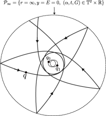
Figure 1.1. Sketch of the projection on the plane of a segment of the diffusive orbit. It shadows a finite family of parabolic orbits which are indeed heteroclinic orbits to $\mathcal{P}_{\infty}$. As the angular momentum grows the massless body $q$ passes further from the primaries.

1.4. Outline of the proof of Theorem 1.1

We introduce the (exact symplectic) change to polar coordinates $(r,y,\alpha,G,t,E)\mapsto(q,p,t,E)$ where $q=(r\cos\alpha,r\sin\alpha)$ and $(y,G)$ are the conjugate momenta to $(r,\alpha)$. In this coordinate system, the RPE3BP is a Hamiltonian system on the (extended) phase space

(1.2) $$(r,\alpha,t,y,G,E)\in\mathbb{R}_{+}\times\mathbb{T}^{2}\times\mathbb{R}^{3}\equiv M_{\mathrm{pol}}$$

with Hamiltonian function

(1.3) $$H_{\mathrm{pol}}(r,\alpha,t,y,G,E)=\frac{y^{2}}{2}+\frac{G^{2}}{2r^{2}}-V_{\mathrm{pol}}(r,\alpha,t)+E,\qquad\qquad V_{\mathrm{pol}}(r,\alpha,t)=U(r\cos\alpha,r\sin\alpha,t).$$

The equations of motion in polar coordinates simply read

$$\dot{r}= \partial_{y}H_{\mathrm{pol}}=y \dot{y}=- \partial_{r}H_{\mathrm{pol}}=\frac{G^{2}}{r^{3}}+\partial_{r}V_{\mathrm{pol}}$$

$$\dot{\alpha}= \partial_{G}H_{\mathrm{pol}}=\frac{G}{r^{2}} \dot{G}=- \partial_{\alpha}H_{\mathrm{pol}}=\partial_{\alpha}V_{\mathrm{pol}}$$

$$\dot{t}= \partial_{E}H_{\mathrm{pol}}=1 \dot{E}=- \partial_{t}H_{\mathrm{pol}}=\partial_{t}V_{\mathrm{pol}}.$$

Since $V_{\mathrm{pol}}(r,\alpha,t)\to 0$ as $r\to\infty$, we identify the invariant submanifold

(1.4) $$\mathcal{P}_{\infty}=\left\{(\infty,\varphi,t,0,I,0)\colon(\varphi,t)\in\mathbb{T}^{2},I\in\mathbb{R}\right\}$$

contained in the zero energy level $\{H_{\mathrm{pol}}=0\}$.

Remark 2.

We have already pointed out in the introduction that, although the Restricted 3 Body Problem with $\mu>0,\epsilon=0$, (i.e. the RPC3BP) is non integrable (see [GMS16]), the existence of topological instability is prevented by the rotational symmetry. In particular, the conservation of the Jacobi constant $\mathtt{J}=H_{\mathrm{pol}}-G$, which is a consequence of the rotational symmetry, readily shows that, for the RPC3BP, there cannot exist heterolicinic orbits connecting periodic orbits in $\mathcal{P}_{\infty}$ with different values of $G$ (see also Lemma 3.9).

However, we want to remark that in the setting in Theorem 1.1 one cannot deduce the existence of transversal intersections between $W^{\mathrm{u}}(\mathcal{P}_{\infty})$ and $W^{\mathrm{s}}(\mathcal{P}_{\infty})$ from that of the invariant manifolds of the RPC3BP. Indeed, the splitting between the invariant manifolds in the case $\mu>0,\epsilon=0$ is exponentially small in $1/G_{*}$ and we consider eccentricities up to polynomially small values in $1/G_{*}$.

Despite being degenerate (the linearized vector field restricted to $\mathcal{P}_{\infty}$ vanishes), it is a classical result of Baldomá and Fontich [BF04b] (see also McGehee [McG73] for the circular case) that the manifold $\mathcal{P}_{\infty}$ posseses stable and unstable manifolds

(1.5) $$\begin{split}W^{\mathrm{u}}(\mathcal{P}_{\infty})=&\{x\in\{H_{\mathrm{pol}}=0\}\colon\exists z\in\mathcal{P}_{\infty}\ \text{ for which }\ \lim_{\tau\to-\infty}|\phi^{\tau}(x)-\phi^{\tau}(z)|=0\}\\ W^{s}(\mathcal{P}_{\infty})=&\{x\in\{H_{\mathrm{pol}}=0\}\colon\exists z\in\mathcal{P}_{\infty}\ \text{ for which }\ \lim_{\tau\to\infty}|\phi^{\tau}(x)-\phi^{\tau}(z)|=0\}.\\ \end{split}$$

By introducing the McGehee transformation $r=\eta_{\mathrm{MG}}(x)=2/x^{2}$, one can prove that the flow on a neighborhood of the invariant manifold $\tilde{\mathcal{P}}_{\infty}=\eta_{\mathrm{MG}}^{-1}(\mathcal{P}_{\infty})$ “behaves” as the flow around a Normally Hyperbolic Invariant Cylinder. Namely, one can prove that $W^{\mathrm{u,s}}(\tilde{\mathcal{P}}_{\infty})=\eta_{\mathrm{MG}}^{-1}(W^{\mathrm{u,s}}(\mathcal{P}_{\infty}))$ exist and are analytic submanifolds except at $x=0$, where they are $C^{\infty}$, and that a parabolic version of the Lambda lemma holds. Because of this, we say that $\mathcal{P}_{\infty}$ is a Topological Normally Hyperbolic Invariant Cylinder (TNHIC).

In order to prove Theorem 1.1, we will use the invariant manifolds of $\mathcal{P}_{\infty}$, whose vertical direction is parametrized by the coordinate $G$, as a highway to obtain orbits whose angular momentum $G$ experiences arbitrarily large variations. More concretely, we build a transition chain of periodic orbits in $\mathcal{P}_{\infty}$ along which $G$ increases.

There are two main ingredients for the construction of the aforementioned transition chain of periodic orbits. The first one is the existence of two different transverse intersections between $W^{\mathrm{u}}(\mathcal{P}_{\infty})$ and $W^{\mathrm{s}}(\mathcal{P}_{\infty})$. The second one is to establish certain transversality property between the dynamics along the two different 3 dimensional homoclinic manifolds associated to the transverse intersections between $W^{\mathrm{u}}(\mathcal{P}_{\infty})$ and $W^{\mathrm{s}}(\mathcal{P}_{\infty})$. The application of these ideas to the RPE3BP, without assuming that $\mu$ is exponentially small with respect to $1/G_{*}$, is quite challenging since major difficulties are present in the verification of each of the two main ingredients for the construction of the transition chain.

Transverse homoclinic intersections between the invariant manifolds for $\mu\in(0,1/2)$:

The existence of transverse intersections between the stable and unstable manifolds of a hyperbolic periodic orbit was already identified by Poincaré as a major source of dynamical complexity (see [Poi90]). The occurrence of this phenomenon, although residual in the $C^{r}$ ($r\geq 1$) topology for vector fields on a compact manifold, is nevertheless rather complicated to check in a particular model and, in general, little can be said except in the case of perturbations of systems with a Normally Hyperbolic Invariant Manifold whose stable and unstable manifolds coincide along a homoclinic manifold.

Our approach to show that the invariant manifolds $W^{\mathrm{u},\mathrm{s}}(\mathcal{P}_{\infty})$ defined in (1.5) intersect transversally is to study the RPE3BP as a small perturbation of the integrable 2BP, in which the invariant manifolds of $\mathcal{P}_{\infty}$ coincide along a homoclinic manifold $W^{\mathrm{h}}_{\mathrm{2BP}}(\mathcal{P}_{\infty})$ of parabolic motions. Yet, for fixed $\mu\in(0,1/2)$, the RPE3BP is far from the 2BP. We however recover a nearly integrable regime if we focus our attention to the region of the phase space $\{G\geq G_{*}\}$ with $G_{*}$ sufficiently large. The reason is that, for $G_{*}$ large enough, the stable and unstable manifolds $W^{\mathrm{u},\mathrm{s}}(\mathcal{P}_{\infty}\cap\{G\geq G_{*}\})$ are located far away from the primaries and therefore, they can be studied as a perturbation of the homoclinic manifold $W^{\mathrm{h}}_{\mathrm{2BP}}(\mathcal{P}_{\infty}\cap\{G\geq G_{*}\})$ (see Section 2). The (substantial) price to pay is that this regime corresponds to a singular perturbation setting. Namely, as we show in Section 2, for $G_{*}\gg 1$, the dynamics in a neighborhood of $W^{\mathrm{u},\mathrm{s}}(\mathcal{P}_{\infty}\cap\{G\geq G_{*}\})$ corresponds to a fast periodic analytic perturbation coupled to the slow dynamics of the integrable 2BP. Indeed, since the Newtonian potential decays with distance, the motion of the massless body is much slower than the rotation of the primaries. The existence of these two time scales results in an exponentially small splitting (in $1/G_{*}\ll 1$) between the invariant manifolds $W^{\mathrm{u}}(\mathcal{P}_{\infty}\cap\{G\geq G_{*}\})$ and $W^{\mathrm{s}}(\mathcal{P}_{\infty}\cap\{G\geq G_{*}\})$: the effect of the perturbation along a neighborhood of the homoclinic manifold $W^{\mathrm{h}}_{\mathrm{2BP}}$ averages out up to an exponentially small remainder which, as a matter of fact, bounds the distance between $W^{\mathrm{u}}(\mathcal{P}_{\infty}\cap\{G\geq G_{*}\})$ and $W^{\mathrm{s}}(\mathcal{P}_{\infty}\cap\{G\geq G_{*}\})$ (see [Nei84]).

In the a priori unstable setting, that is, perturbations of systems with a Normally Hyperbolic Invariant Manifold whose stable and unstable manifolds coincide along a homoclinic manifold, and for which the hyperbolicity is much stronger than the size of the perturbation, there are no different time scales. Therefore, the splitting between invariant manifolds is usually tackled by means of Poincaré-Melnikov theory (see [Mel63, DdlLS06, GdlL18]), which gives an asymptotic formula for the distance between them in terms of a convergent improper integral, usually referred to in the literature as the Melnikov function. Nevertheless, establishing the validity of the Melnikov approximation in the singular perturbation framework where the splitting between $W^{\mathrm{u},\mathrm{s}}$ is exponentially small (as is the case of the present problem), is a demanding problem for which no general theory is available.

One should remark that the original Arnold model, despite having two different time scales, it possesses two parameters: the one measuring the ratio between time scales $\varepsilon$ and the one measuring the size of the perturbation $\mu$. In this case, Melnikov theory predicts that $\mathrm{dist}(W^{\mathrm{u}},W^{\mathrm{s}})\sim M+\mathcal{O}(\mu^{2})$ for a function $M$ which “typically” has size $M\sim\mu\exp(-c/\sqrt{\varepsilon})$. Therefore, by assuming that the size of the perturbation $\mu$ is exponentially small compared to the ratio between time scales, classical Melnikov theory can be directly applied even if the splitting between $W^{\mathrm{u},\mathrm{s}}$ is exponentially small in $\varepsilon$. This was the approach considered in [Arn64] and [DKdlRS19].

The analysis of exponentially small splitting has drawn major attention in the past decades due to its relevance for the study of instability mechanisms in real analytic Hamiltonian systems. Indeed, in the absence of extra perturbative parameters, as is the case in a priori stable systems (perturbations of integrable systems in action angle variables: no hyperbolicity is present in the integrable system), one has to face this phenomenon. Remarkable progress has been made in a number of works in low dimensional models (just to cite a few works, see [Laz87, DS92, Gel94, Gel97, Tre97, Gel99, BF04a, MSS11, BFGS12, Gua13]). In higher dimension, results are much more scarce. We highlight [Sau01] and [LMS03], where the exponentially small splitting between the stable and unstable manifolds of a partially hyperbolic invariant torus is investigated. When the torus under consideration is sufficiently irrational, the splitting of its invariant manifolds is exponentially small in all directions (see [DGJS97] and [Sau01]). However, if the torus is resonant, one expects that the splitting is in general highly anisotropic, involving directions in which the splitting is exponentially small and directions in which the splitting is of the order of the perturbation. This strong anisotropy complicates heavily the geometric analysis. Exponentially small splitting happens in directions close to that of the actions conjugated to the fast angles and polynomially small splitting happens in directions close to that of the actions conjugated to the resonant angles. However is not clear a priori how to locate exactly the directions of exponentially small splitting.

In [LMS03], Lochak, Marco and Sauzin developed a formalism to identify the directions of exponentially small splitting between the stable and unstable manifolds of the same partially hyperbolic invariant torus. The situation is much more intrincate when one considers the invariant manifolds associated to two different partially hyperbolic invariant tori. Indeed, all previous works which study the existence of transverse intersections between the invariant manifolds of different invariant tori rely on an indirect approach: first, one proves the existence of transverse homoclinic intersections between the invariant manifolds of a given torus and then deduce the existence of heteroclinic connections between nearby tori by direct application of the implicit function theorem. However, the directions along which the splitting is exponentially small can move as we vary the torus. Therefore, to ensure that all the errors in the approximation by the homoclinic connection are exponentially small, this indirect method only works when the two tori under consideration are exponentially close.

The present is, to the best of the authors knowledge, the first work in which the highly anisotropic splitting between the invariant manifolds of a pair of partially hyperbolic fully resonant invariant tori (which in the current problem foliate $\mathcal{P}_{\infty}$) is succesfully analyzed. Namely, by studying the problem in a direct way we establish the existence of heteroclinic connections between resonant tori separated up to a distance of the size of the perturbation. This allows us to prove the existence of two manifolds $\Gamma_{\pm}$ of homoclinic points to $\mathcal{P}_{\infty}\cap\{t=0\}$ which moreover are diffeomorphic to

$$\mathcal{P}_{\infty}^{*}=\mathcal{P}_{\infty}\cap\{t=0,\ G_{*}<G<\epsilon^{-1/3}\}.$$

The main idea behind our approach is to exploit the Hamilton-Jacobi formalism for, given a pair of partially hyperbolic invariant tori, building a local symplectic coordinate system, tailored made for each pair of invariant tori, in which the direction of exponentially small splitting between their associated invariant manifolds is clearly isolated from the non-exponentially small one. The coordinate system strongly depends on the pair of tori considered, what gives an idea of the subtleness of the phenomenon. The key player in this construction is the “splitting potential” $\Delta S$, which will be defined in (3.13) as the difference between the generating function of the unstable manifold of one of the tori and the generating function of the stable manifold of the other torus .

Remark 3.

The splitting potential was first introduced by Eliasson in [Eli94] and later appeared in the work of Sauzin [Sau01] and Lochak, Marco and Sauzin [LMS03], to study the splitting between the invariant manifolds of a given torus. The terminology splitting potential was coined in [DG00].

In the variational approach to Arnold Diffusion, the splitting potential also plays a major role, since it is related to the so called Peierl’s barrier in Mather theory (see [Zha11]).

Another remarkable novelty of our construction is that we work directly with the generating functions associated to the stable and unstable manifolds of the invariant tori instead of relying on a vector parametrization of these invariant manifolds. The difficulty to work directly with the generating function is the appearance of certain unbounded operator in the linearized invariance equation which defines the generating functions (see [Sau01]). This obstacle was removed in all previous works by considering a different vector parametrization of the invariant manifolds. We overcome the problem, and directly find the generating functions, by making use of a suitable Newton iterative scheme in a scale of Banach spaces in the spirit of the usual schemes used in KAM theory.

Construction of a transition chain of heteroclinic orbits:

The progress made in the analysis of the strongly anisotropic splitting between invariant manifolds of partially hyperbolic resonant invariant tori is of high relevance for the second step in the proposed diffusion mechanism. Indeed, we are able to prove that the scattering maps (see [DdlLS08]), which encode the dynamics along the homoclinic manifolds $\Gamma_{\pm}$, are globally defined on $\mathcal{P}_{\infty}^{*}\subset\mathcal{P}_{\infty}$. This result was already obtained in [DKdlRS19], for the a priori unstable case $\mu\ll\exp(-G_{*}^{3}/3)$ and is extended in this work to the a priori stable setting $\mu\in(0,1/2)$. Besides the importance of this achievement for the study of Arnold Diffusion in a priori stable Hamiltonians, the existence of two globally defined scattering maps is vital for the construction of diffusive orbits in the RPE3BP. As a matter of fact, the inner dynamics on $\mathcal{P}_{\infty}$ is trivial and, as seen in [DKdlRS19], we can only rely on the combination of the two scattering maps.

The pair of scattering maps on $\mathcal{P}_{\infty}^{*}$ defines an iterated function system: the existence of a transition chain of heteroclinic orbits to $\mathcal{P}_{\infty}$, along which the drift in the angular momentum $G$ takes place, is guaranteed after showing that the two scattering maps share no common invariant curves (see [Moe02] and also [LC07]). This is a rather challenging problem since, although both scattering maps are only polynomially close (in $1/G_{*}$) to the identity, the difference between them averages out up to an exponentially small quantity (in $1/G_{*}$) which, we show, is different from zero on an open subset of $\mathcal{P}^{*}_{\infty}$.

The key to establish this result is the construction of a generating function for each scattering map, which are exact symplectic. We moreover show that the asymptotics of these generating functions are well controlled by the asymptotics of an explicit function usually referred to as the reduced Melnikov potential. Once the dynamics of both scattering maps have been distinguished, we apply an interpolation result combined with an averaging procedure to show that the invariant curves of both maps always intersect transversally.

1.5. A degenerate Arnold model

Since we expect that the ideas of this work can be of interest for readers from the field of Arnold diffusion, but which might have no background in Celestial Mechanics, in this section we present a degenerate version of the Arnold model (see [Arn64]) which illustrates the two main challenges we face.

Consider the Hamiltonian system

(1.6) $$H(q,p,\varphi,I,t;\varepsilon,\mu)=H_{0}(q,p,I;\varepsilon)+\mu H_{1}(q,\varphi,t;\varepsilon),\quad\qquad(q,p)\in\mathbb{T}\times\mathbb{R},\ (\varphi,I)\in\mathbb{T}\times\mathbb{R},\ t\in\mathbb{T}$$

where

$$H_{0}(q,p,I;\varepsilon)=\frac{p^{2}}{2}+\varepsilon(\cos q-1)\left(1+\frac{I^{2}}{2}\right),\qquad\qquad H_{1}(q,\varphi,t;\varepsilon)=\varepsilon(\cos q-1)\left(\sin\varphi+\cos t\right).$$

We observe that, for any $\mu,\varepsilon\geq 0$,

$$\mathcal{N}=\{(q,p,\varphi,I,t)\in\mathbb{T}\times\mathbb{R}\times\mathbb{T}\times\mathbb{R}\times\mathbb{T}\colon q=p=0\}$$

is a Normally Hyperbolic Invariant Cylinder, which is foliated by periodic orbits with frequencies

$$(\omega_{\varphi},\omega_{t})=(0,1).$$

Due to the fact that the inner dynamics on $\mathcal{N}$ is trivial, in order to obtain orbits which present a large drift along the $I$ component, we can only rely on the outer dynamics.

The setting $0<\varepsilon\ll 1$ and $0<\mu\ll\exp(-1/\sqrt{\varepsilon})$, which corresponds to the so called a priori unstable case, can be identified (up to major difficulties and technicalities associated to the particular form of the Hamiltonian of the RPE3BP) with the situation studied in [DKdlRS19]. Define

$$\tilde{\varepsilon}=\varepsilon\left(1+\frac{I^{2}}{2}\right).$$

When $\mu=0$, the system has an homoclinic manifold to $\mathcal{N}$ which can be parametrized as

$$\Gamma_{\mathrm{h}}(s,\theta,I;\tilde{\varepsilon})=\{(q,p,\varphi,I)=(q_{\mathrm{h}}(s),\sqrt{\tilde{\varepsilon}}p_{\mathrm{h}}(s),\theta+\theta_{\mathrm{h}}(s,I;\sqrt{\tilde{\varepsilon}}),I),\ s\in\mathbb{R},\ (\theta,I)\in\mathbb{T}\times\mathbb{R}\}\quad\text{with}\quad\dot{s}=1/\sqrt{\tilde{\varepsilon}}.$$

By assuming that $\mu\ll\exp(-1/\sqrt{\tilde{\varepsilon}})$, one can use classical perturbation theory to show that, $W^{\mathrm{u}}(\mathcal{N})$ and $W^{\mathrm{s}}(\mathcal{N})$ intersect transversally along two different homoclinic manifolds $\Gamma_{\pm}$. Indeed, as explained in the previous section, Poincaré-Melnikov theory predicts that, when measured along the line orthogonal to the unperturbed homoclinic manifold and passing through the point $(\Gamma_{\mathrm{h}}(s,\theta,I;\tilde{\varepsilon}),t)$, the distance between the invariant manifolds is given by

$$\mathrm{dist}(W^{\mathrm{u}}(\mathcal{N}),W^{\mathrm{s}}(\mathcal{N}))\sim\mu\partial_{s}\mathcal{L}(\theta,I,t-s/\sqrt{\tilde{\varepsilon}};\tilde{\varepsilon})+\mathcal{O}(\mu^{2}),$$

where

$$\mathcal{L}(\theta,I,\sigma;\tilde{\varepsilon})=\frac{1}{\sqrt{\tilde{\varepsilon}}}\int_{-\infty}^{\infty}H_{1}(q_{\mathrm{h}}(\tau),\sqrt{\tilde{\varepsilon}}p_{\mathrm{h}}(\tau),\theta+\theta_{\mathrm{h}}(\tau,I;\sqrt{\tilde{\varepsilon}}),\sigma+\tau/\sqrt{\tilde{\varepsilon}})\mathrm{d}\tau,$$

is the so-called Melnikov potential. Using the expression for $H_{1}$, one can easily see that

$$\partial_{s}\mathcal{L}(\theta,I,t-s/\sqrt{\tilde{\varepsilon}};\tilde{\varepsilon})=\frac{2\pi}{\sinh\left(\frac{\pi}{2\sqrt{\tilde{\varepsilon}}}\right)}\sin\left(t-s/\sqrt{\tilde{\varepsilon}}\right)=\mathcal{O}(\exp(-1/\sqrt{\tilde{\varepsilon}}).$$

The claim then follows from the fact that, for all $(\theta,I,t)\in\mathbb{T}\times\mathbb{R}\times\mathbb{T}$, there exist two different non-degenerate zeros $s_{+}(t,I)=\sqrt{\tilde{\varepsilon}}t$ and $s_{-}(t,I)=\sqrt{\tilde{\varepsilon}}t+\pi$ of the function $s\mapsto\partial_{s}\mathcal{L}(\theta,I,t-s/\sqrt{\tilde{\varepsilon}};\tilde{\varepsilon})$.

This allows to define two scattering maps $\mathbb{P}_{\pm}:\mathcal{N}\cap\{t=0\}\to\mathcal{N}\cap\{t=0\}$, associated to the homoclinic manifolds $\Gamma_{\pm}$. Finally, one can show (see [DdlLS08]) that the dynamics of each of the scattering maps $\mathbb{P}_{\pm}$ expressed in variables $(\theta,I)$, are given by

$$\mathbb{P}_{\pm}=\mathrm{Id}+\mu\mathcal{J}\nabla\mathcal{L}_{\pm}(\theta,I;\tilde{\varepsilon})+\mathcal{O}(\mu^{2}),$$

where $\mathcal{J}$ is the standard complex structure in $\mathbb{R}^{2}$ and

$$\mathcal{L}_{\pm}(\theta,I;\tilde{\varepsilon})=\mathcal{L}(\theta,I,-s_{\pm}(0,I)/\sqrt{\tilde{\varepsilon}};\tilde{\varepsilon}).$$

Therefore, in the case $\mu\ll\exp(-1/\sqrt{\tilde{\varepsilon}})$, classical perturbation theory yields an asymptotic formula for the difference between $\mathbb{P}_{+}$ and $\mathbb{P}_{-}$ which can be used to verify the existence of drifting orbits.

The problem is much more intrincate if $\mu\sim\tilde{\varepsilon}^{\alpha}$ (for a given $\alpha>0$). On one hand, as already explained in Section 1.4, one cannot make use of classical perturbation theory to study directly the existence of transverse intersections between $W^{\mathrm{u},\mathrm{s}}(\mathcal{N})$. The ideas developed in [Sau01] and [LMS03] could be used to prove the existence of two functions $\theta_{\pm}(I^{\prime})$ such that for every $I^{\prime}$, $(q,p,\varphi,I,t)=(0,0,\theta_{\pm}(I^{\prime}),I^{\prime},0)\subset\mathcal{N}$ is a point for which there exist a homoclinic orbit to the torus $\mathcal{T}_{I^{\prime}}=\mathcal{N}\cap\{I=I^{\prime}\}$. Then, by application of the implicit function theorem, one can show that there exist two scattering maps $\mathbb{P}_{\pm}:\mathcal{N}_{\pm}\cap\{t=0\}\to\mathcal{N}\cap\{t=0\}$ where $\mathcal{N}_{\pm}$ are vertical strips of the form

$$\mathcal{N}_{\pm}=\{(q,p,\varphi,I,t)\in\mathbb{T}\times\mathbb{R}\times\mathbb{T}\times\mathbb{R}_{+}\times\mathbb{T}\colon q=p=0,\ |\varphi-\theta_{\pm}(I)|\leq\exp(-1/\sqrt{\tilde{\varepsilon}})\}.$$

However, with this approach $\mathcal{N}_{+}\cap\mathcal{N}_{-}=\emptyset$. Therefore, only one scattering map would be available on each domain and diffusion would be prevented by the existence of invariant curves of the scattering maps. The ideas we introduce in the present work allow us to prove the existence of two globally defined scattering maps $\mathbb{P}_{\pm}:\mathcal{N}\cap\{t=0\}\to\mathcal{N}\cap\{t=0\}$ in the case $\mu\sim\tilde{\varepsilon}^{\alpha}$.

Finally, in the case $\mu\sim\tilde{\varepsilon}^{\alpha}$, both scattering maps $\mathbb{P}_{\pm}$ are only $\mathcal{O}(\tilde{\varepsilon}^{\beta})$ (for some $\beta>0$) close to the identity whereas the difference between $\mathbb{P}_{+}$ and $\mathbb{P}_{-}$ averages out to up to an exponentially small $\sim\mu\exp(-1/\sqrt{\tilde{\varepsilon}})$ term (the size of the splitting). Therefore, proving that this difference is not zero, is much more demanding than in the a priori unstable case $\mu\ll\exp(-1/\sqrt{\tilde{\varepsilon}})$ (even $\mu=1$).

We end this section with two remarks concerning the degeneracy of Hamiltonian (1.6) (and of the setting in which we build the diffusion mechanism leading to Theorem 1.1). The first one is that the convexity of (1.6) close to $\mathcal{N}$ is of order $\varepsilon$ (and vanishes on $\mathcal{N}$). Therefore, the Hamiltonian (1.6) does not satisfy the assumptions of Nekhoroshev theorem and one could think that the diffusion time is polynomial in $\varepsilon$. This is not the case since the angle between the invariant curves of the map $\mathbb{P}_{+}$ and those of the map $\mathbb{P}_{-}$ is exponentially small with respect to $\varepsilon$.

The second remark is that, although in the present case all the cylinder is foliated by periodic orbits with the same frequency (which, as already discussed above, introduces certain challenges for proving the existence of diffusive orbits), we have the strong feeling that the the ideas developed in this work, specially the ones in Sections 3.1 and 3.3, can be adapted to the a priori stable case for the original Arnold model, in which there exists a Normally Hyperbolic Invariant Cylinder $\widetilde{\mathcal{N}}$ foliated by invariant tori of frequencies $(\omega_{\varphi}(I),\omega_{t})=(I,1)$.

1.6. Organization of the article

In Section 2 we introduce the (nearly integrable) parabolic regime with large angular momentum discussed in Section 1.4. We show that, in this regime, the RPE3BP can be treated as a fast time periodic perturbation of the 2BP, whose main features are also discussed in Section 2. Section 3 contains the core of the proof of Theorem 1.1. More concretely, Section 3.1 renders the main ideas behind the proof of the first main ingredient: existence of transverse intersections between the invariant manifolds of $\mathcal{P}_{\infty}$. The proof of this result is postponed to Section 4. Sections 3.2 to 3.5 are devoted to the construction of two global scattering maps on $\mathcal{P}_{\infty}$ and the analysis of the transversality between the invariant curves of these maps. The rather technical proofs of the results in these sections are deferred to Sections 5, 6 and Appendix B. Finally, in Section 3.6 we state a suitable shadowing result for parabolic manifolds which completes the proof of Theorem 1.1. Appendix A contains a detailed study of the perturbative potential and the associated Melnikov potential.

Througout the rest of the paper we fix a value $\mu\in(0,1/2)$.

Aknowledgements

This project has received funding from the European Research Council (ERC) under the European Union’s Horizon 2020 research and innovation programme (grant agreement No 757802). This work is part of the grant PID-2021-122954NB-100 funded by MCIN/AEI/10.13039/501100011033 and “ERDF A way of making Europe”. M.G. and T.M.S are supported by the Catalan Institution for Research and Advanced Studies via an ICREA Academia Prize 2019. This work is also supported by the Spanish State Research Agency, through the Severo Ochoa and María de Maeztu Program for Centers and Units of Excellence in R&D (CEX2020-001084-M).

2. The 2BP and a nearly integrable regime for the RPE3BP

The 2 Body Problem (2BP) in polar coordinates is the Hamiltonian system associated to

(2.1) $$H_{\mathrm{2BP}}(r,y,G)=\frac{y^{2}}{2}+\frac{G^{2}}{2r^{2}}-\frac{1}{r}$$

on the phase space $(r,\alpha,y,G)\in\mathbb{R}_{+}\times\mathbb{T}\times\mathbb{R}^{2}$. Since the Hamiltonian $H_{\mathrm{2BP}}$ does not depend on the angle $\alpha$, the angular momentum $G$ is a first integral for the 2BP. Moreover, it is functionally independent and commutes with the energy $H_{\mathrm{2BP}}$, what makes the 2BP integrable. The dynamics of the 2BP is completely understood: positive energy levels correspond to hyperbolic motions, negative energy levels to elliptic motions and the zero energy level corresponds to parabolic motions.

2.1. The parabolic homoclinic manifold of the 2BP

Of special interest for us are the parabolic motions. Denote by $\mathcal{P}_{\infty}^{\mathrm{2BP}}=\{(\infty,\alpha,0,G)\in\mathbb{R}_{+}\times\mathbb{T}\times\mathbb{R}^{2}\}=\mathcal{P}_{\infty}\cap\{t=E=0\}$ the parabolic infinity in the reduced phase space (see the extended phase space in polar coordinates in Section 1.1), which is a 2 dimensional TNHIC. Then, the set of points leading to parabolic motions, that is, the set $\{H_{\mathrm{2BP}}=0\}$, is a 3 dimensional submanifold $W^{\mathrm{h}}_{\mathrm{2BP}}$ homoclinic to $\mathcal{P}_{\infty}^{\mathrm{2BP}}$. Let $\phi^{\tau}_{H_{\mathrm{2BP}}}$ be the flow associated to the Hamiltonian (2.1), then

(2.2) $$W^{\mathrm{h}}_{\mathrm{2BP}}=\{x\in\mathbb{R}_{+}\times\mathbb{T}\times\mathbb{R}^{2}\colon\exists z\in\mathcal{P}_{\infty}^{\mathrm{2BP}}\quad\text{for which}\quad\lim_{\tau\pm\infty}|\phi^{\tau}_{H_{\mathrm{2BP}}}(x)-\phi^{\tau}_{H_{\mathrm{2BP}}}(z)|=0\}.$$

The following lemma gives a parametrization of the homoclinic manifold $W^{\mathrm{h}}_{\mathrm{2BP}}$. A proof can be found in [MP94].

Lemma 2.1.

There exist real analytic functions $r_{\mathrm{h}}(u),\alpha_{\mathrm{h}}(u)$ and $y_{\mathrm{h}}(u)$ such that

$$W^{\mathrm{h}}_{\mathrm{2BP}}=\{\Gamma_{\mathrm{2BP}}(u,\beta)=(G^{2}r_{\mathrm{h}}(u),\beta+\alpha_{\mathrm{h}}(u),G^{-1}y_{\mathrm{h}}(u),G)\in\mathbb{R}_{+}\times\mathbb{T}\times\mathbb{R}^{2}\colon u\in\mathbb{R},\ \beta\in\mathbb{T},\ G\in\mathbb{R}\setminus\{0\}\}$$

and, if we denote by $X_{\mathrm{2BP}}$ the vector field associated to the Hamiltonian (2.1),

$$X_{\mathrm{2BP}}\circ\Gamma_{\mathrm{2BP}}=D\Gamma_{\mathrm{2BP}}\ \Upsilon\qquad\qquad\text{with}\qquad\qquad\Upsilon=(G^{-3},0).$$

The functions $r_{\mathrm{h}},y_{\mathrm{h}}$ and $\alpha_{\mathrm{h}}$ admit a unique analytic extension to $\mathbb{C}\setminus\{u=is\colon s\in(-\infty,-1/3]\cup[1/3,\infty)\}$ and satisfy the asymptotic behavior

$$r_{\mathrm{h}}(u)\sim u^{2/3}\qquad\qquad\exp(i\alpha_{\mathrm{h}}(u))\sim 1\qquad\qquad y_{\mathrm{h}}(u)\sim u^{-1/3}\qquad\qquad\text{as}\quad u\to\pm\infty$$

and

$$r_{\mathrm{h}}(u)\sim(u\pm i/3)^{1/2}\qquad\quad\exp(i\alpha_{\mathrm{h}}(u))\sim\left(\frac{u\pm i/3}{u\mp i/3}\right)^{1/2}\qquad\quad y_{\mathrm{h}}(u)\sim(u\pm i/3)^{-1/2}\quad\qquad\text{as}\quad u\to\pm i/3.$$

Moreover, $y_{\mathrm{h}}(u)=0$ if and only if $u=0$ and $r_{\mathrm{h}}(u)\geq 1/2$ for all $u\in\mathbb{R}$.

2.2. The parabolic regime with large angular momentum for the RPE3BP

It is a fact, implied by the last item in Lemma 2.1, that, for $G_{*}\gg 1$,

$$\pi_{r}\left(W^{\mathrm{h}}_{\mathrm{2BP}}\cap\{G\geq G_{*}\}\right)\geq G_{*}^{2}/2\gg 1,$$

where by $\pi_{r}$ we denote the projection into the $r$ coordinate. Therefore, in a neighborhood of the parabolic homoclinic manifold (2.2) for the 2BP we have $r\gg 1$ (that is, the massless body is far away from the primaries) and the Hamiltonian of the RPE3BP can be studied as a perturbation of the (integrable) 2BP. Indeed, expanding the Hamiltonian (1.3) in powers of $1/r$,

$$H_{\mathrm{pol}}(r,\alpha,t,y,G,E)=\frac{y^{2}}{2}+\frac{G^{2}}{2r^{2}}-\frac{1}{r}+E+\mathcal{O}\left(\frac{1}{r^{3}}\right)=H_{\mathrm{2BP}}(r,y,G)+E+\mathcal{O}\left(\frac{1}{r^{3}}\right),$$

where we have used that $V_{\mathrm{pol}}$ in (1.3) is given by

$$\begin{split}V_{\mathrm{pol}}(r,\alpha,t)=&\frac{\mu}{(r^{2}+2(1-\mu)r\varrho(t)\cos(\alpha-f(t))+(1-\mu)^{2}\varrho^{2})^{1/2}}\\ &+\frac{1-\mu}{(r^{2}+2\mu r\varrho(t)\cos(\alpha-f(t))+\mu^{2}\varrho^{2})^{1/2}}=\frac{1}{r}+\mathcal{O}\left(\frac{1}{r^{3}}\right).\end{split}$$

With the object of investigating this perturbative regime, we consider an arbitrarily large constant $G_{*}\gg 1$ and make the conformally symplectic scaling

$$(\tilde{r},\alpha,t,\tilde{y},\tilde{G},\tilde{E})\longmapsto(r,\alpha,t,y,G,E)$$

defined by

$$r=G_{*}^{2}\tilde{r},\qquad y=G_{*}^{-1}\tilde{y},\qquad G=G_{*}\tilde{G},\qquad E=G_{*}\tilde{E}.$$

Up to time reparametrization, the autonomous Hamiltonian in the scaled variables reads

$$\tilde{H}(\tilde{r},\alpha,t,\tilde{y},\tilde{G},\tilde{E})=\frac{\tilde{y}^{2}}{2}+\frac{\tilde{G}^{2}}{2\tilde{r}^{2}}-\tilde{V}\left(\tilde{r},\alpha,t\right)+G_{*}^{3}\tilde{E},\qquad\qquad\tilde{V}(\tilde{r},\alpha,t)=G_{*}^{2}V_{\mathrm{pol}}\left(G_{*}^{2}\tilde{r},\alpha,t\right).$$

It is an easy computation to show that, for $G_{*}^{2}\tilde{r}\gg 1$,

$$\tilde{V}(\tilde{r},\alpha,t)=\frac{1}{\tilde{r}}+\mathcal{O}\left(\frac{1}{G_{*}^{4}\tilde{r}^{3}}\right)$$

and, therefore

$$\tilde{H}(\tilde{r},\alpha,t,\tilde{y},\tilde{G},\tilde{E})=H_{\mathrm{2BP}}(\tilde{r},\tilde{y},\tilde{G})+G_{*}^{3}\tilde{E}+\mathcal{O}(G_{*}^{-4}\tilde{r}^{-3}).$$

The nature of this perturbative regime is now clear: in the parabolic regime with large angular momentum the RPE3BP is a fast time periodic perturbation ($\dot{t}=G_{*}^{3}$) of the slow dynamics ($\dot{\tilde{r}}\sim\dot{\alpha}\sim\dot{\tilde{y}}=\mathcal{O}(1)$) of the 2BP. Since the gravitational potential $\tilde{V}$ is analytic on a complex neighborhood of the embedding of $W^{\mathrm{h}}_{\mathrm{2BP}}$ in the extended phase space, succesive averaging steps can be performed to find a real analytic change of variables $\psi$ defined on a complex neighborhood of $W^{\mathrm{h}}_{\mathrm{2BP}}\cap\{\tilde{G}\geq 1\}$ in which

(2.3) $$\tilde{H}\circ\psi=K+\mathcal{O}(\exp(-CG_{*}^{3}))$$

for some $C>0$ and where $K=K(\tilde{r},\alpha,\tilde{y},\tilde{G})$ is $\mathcal{O}(G_{*}^{-4})$ close to $\tilde{H}$ and coincides with $\tilde{H}$ at $\mathcal{P}_{\infty}\cap\{\tilde{G}\geq 1\}$. A simple counting dimension argument shows that, for the flow associated to the 2 degrees of freedom autonomous Hamiltonian $K$, the invariant manifolds associated to $\mathcal{P}_{\infty}\cap\{\tilde{G}\geq 1\}$ (which is also a TNHIC for $K$) must coincide along a homoclinic manifold. Therefore, it follows from (2.3) that the distance between $W^{\mathrm{u},\mathrm{s}}(\mathcal{P}_{\infty}\cap\{G\geq G_{*}\})$ is bounded by $\mathcal{O}(\exp(-CG_{*}^{3}))$.

3. Proof of the main theorem

The first step in the proof of Theorem 1.1 is to prove that the manifolds $W^{\mathrm{u},\mathrm{s}}(\mathcal{P}_{\infty})$ (defined in (1.5)) intersect transversally. This is a rather delicate problem since we will see that the splitting angle between $W^{\mathrm{u}}(\mathcal{P}_{\infty}\cap\{G\geq G_{*}\})$ and $W^{\mathrm{s}}(\mathcal{P}_{\infty}\cap\{G\geq G_{*}\})$ is exponentially small in $1/G_{*}$ and we will not study directly the existence of intersections between them. The reason is that, in order to measure this splitting, one needs to find a suitable local coordinate system which isolates the exponentially small directions. However, these directions are highly sensitive with respect to the projection along the stable and unstable foliations (see Figure 3.1) and it is not clear a priori how to locate them without exploiting the symplectic features of the problem.

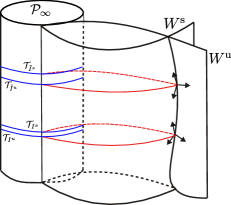
Figure 3.1. The unstable and stable manifolds $W^{\mathrm{u,s}}(\mathcal{P}_{\infty})$ of the Topological Normally Hyperbolic Invariant Cylinder $\mathcal{P}_{\infty}$. In order to measure the splitting between $W^{\mathrm{u}}_{I^{\mathrm{u}}}$ and $W^{s}_{I^{\mathrm{s}}}$ we build a suitable symplectic coordinate system (depending non trivially on $I^{\mathrm{u}}$ and $I^{\mathrm{s}}$), in which the directions of exponentially small splitting are isolated from the non-exponentially small one.

To overcome this difficulty we take advantage of the fact that $\mathcal{P}_{\infty}$ in (1.4) is foliated by invariant tori

$$\mathcal{P}_{\infty}=\bigcup_{I\in\mathbb{R}}\mathcal{T}_{I},\qquad\qquad\mathcal{T}_{I}=\left\{x=(\infty,\varphi,t,0,I,0),\ (\varphi,t)\in\mathbb{T}^{2},\ G=I\right\}$$

and, therefore, we can express

$$W^{\mathrm{u},\mathrm{s}}(\mathcal{P}_{\infty})=\bigcup_{I\in\mathbb{R}}W_{I}^{\mathrm{u},\mathrm{s}}$$

where $W_{I}^{\mathrm{u},\mathrm{s}}$ are the stable and unstable manifolds of the invariant torus $\mathcal{T}_{I}$. Since $W^{\mathrm{u},\mathrm{s}}_{I}$ are Lagrangian submanifolds, one can parametrize them (at least locally) as a graph over the configuration space and measure the splitting in the conjugate directions. Since all tori $\mathcal{T}_{I}\subset\mathcal{P}_{\infty}$ are resonant with frequencies $(\omega_{\alpha},\omega_{t})=(0,1)$, we will see that the splitting between their invariant manifolds is highly anisotropic.

In the present work, we extend the formalism developed by Lochak, Marco and Sauzin in [LMS03], to analyze directly the existence of transverse intersections between the stable $W^{\mathrm{s}}_{I^{\mathrm{s}}}$ and unstable $W^{\mathrm{u}}_{I^{\mathrm{u}}}$ manifolds of two (possibly) different invariant tori $\mathcal{T}_{I^{\mathrm{u}}}$ and $\mathcal{T}_{I^{\mathrm{s}}}$.

3.1. The non exact Lagrangian intersection problem

In this section, we exploit the Hamilton-Jacobi formalism to reduce the problem of existence of intersections between $W^{\mathrm{s}}_{I^{\mathrm{s}}}$ and $W^{\mathrm{u}}_{I^{\mathrm{u}}}$, to the problem of existence of critical points of a certain scalar function. Before entering the details of our construction, the introduction of some notation is in order. Given a value $I_{*}\in\mathbb{R}_{+}$, for $\epsilon\in(0,I_{*}^{-3})$, we define the annulus

(3.1) $$\Lambda(I_{*},\epsilon)=\mathbb{T}\times\{I_{*}\leq I\leq\epsilon^{-1/3}\}\subset\mathbb{T}\times\mathbb{R}$$

and, given $\rho>0$, we introduce the complex neighborhood

(3.2) $$\Lambda_{\rho}(I_{*},\epsilon)=\mathbb{T}_{\rho}\times\Lambda_{\rho,I}(I_{*},\epsilon)\subset(\mathbb{C}/2\pi\mathbb{Z})\times\mathbb{C}$$

where $\mathbb{T}_{\rho}$ is the strip of width $\rho$ centered at the real torus and

(3.3) $$\Lambda_{\rho,I}(I_{*},\epsilon)=\{I\in\mathbb{C}\colon|\mathrm{Im}I|\leq\rho,\ I_{*}\leq\mathrm{Re}I\leq\epsilon^{-1/3}\}.$$

Remark 4.

In the following we will restrict our analysis to tori $\mathcal{T}_{I^{\mathrm{u},\mathrm{s}}}$ such that $I^{\mathrm{u}},I^{\mathrm{s}}\in\Lambda(I_{*},\epsilon)$. The introduction of the annulus $\Lambda(I_{*},\epsilon)\subset\mathbb{T}\times\mathbb{R}$ is needed for the following reasons. On one hand, in order to work in the perturbative regime introduced in Section 2.2, one needs to consider a region of the phase space with sufficiently large angular momentum, hence the requirement $I\geq I_{*}$. On the other hand, the requirement $\epsilon\leq I_{*}^{-3}$ is of technical nature and it is related to the limitations of the method (see Appendix A) that we use to compute the so-called Melnikov potential (defined in (3.15) below).

Remark 5.

The use of complex neighborhoods of $\Lambda(I_{*},\epsilon)$ is needed to make use of Cauchy estimates in Section 3.2. In the following, fixed a value of $I_{*}$, we will simply write $\Lambda,\Lambda_{\rho}$ and $\Lambda_{\rho,I}$ and drop the dependence on $I_{*}$.

Given $I_{*},\rho>0$ and $\epsilon\in(0,I_{*}^{-3})$, for any $I^{\mathrm{u}},I^{\mathrm{s}}\in\Lambda_{\rho,I}$, we define

(3.4) $$I_{\mathrm{m}}=\frac{1}{2}(I^{\mathrm{u}}+I^{\mathrm{s}})$$

and perform the change of variables (depending on $I_{\mathrm{m}}$)

(3.5) $$\eta_{I_{\mathrm{m}}}:(u,\beta,t,Y,J,E;I_{\mathrm{m}})\longmapsto(r,\alpha,t,y,G,E)$$

given by

$$r=I_{\mathrm{m}}^{2}r_{\mathrm{h}}(u)\quad\quad\alpha=\beta+\alpha_{\mathrm{h}}(u)\quad\quad y=I_{\mathrm{m}}^{-1}y_{\mathrm{h}}(u)+I_{\mathrm{m}}^{-2}y_{\mathrm{h}}^{-1}(u)(Y-r_{\mathrm{h}}^{-2}J)\quad\quad G=I_{\mathrm{m}}+J,$$

where $r_{\mathrm{h}},y_{\mathrm{h}}$ and $\alpha_{\mathrm{h}}$ are defined in Lemma 2.1. The change of variables $\eta_{I_{\mathrm{m}}}$ is the symplectic completion of the change in the basis given by $r=I_{\mathrm{m}}^{2}r_{\mathrm{h}}(u)$, $\alpha=\beta+\alpha_{\mathrm{h}}(u)$, which is well suited to study a neighborhood of the unperturbed homoclinic orbit $W^{\mathrm{h}}_{\mathrm{2BP}}\cap\{G=I_{\mathrm{m}}\}$ (see (2.2)).

A key point in our construction, is that we use the parametrization of $W^{\mathrm{h}}_{\mathrm{2BP}}\cap\{G=I_{\mathrm{m}}\}$ in Lemma 2.1 as first order approximation both for the unstable manifold of $\mathcal{T}_{I^{\mathrm{u}}}$ and for the stable manifold of $\mathcal{T}_{I^{\mathrm{s}}}$.

Remark 6.

Notice that in $(u,\beta,t,Y,J,E)$ coordinates, the tori $\mathcal{T}_{I^{\mathrm{u},\mathrm{s}}}$ are given by $\mathcal{T}_{I^{\mathrm{u}}}=\{u=-\infty,Y=E=0,\ J=I^{\mathrm{u}}-I_{\mathrm{m}}\}$ and $\mathcal{T}_{I^{\mathrm{s}}}=\{u=\infty,Y=E=0,\ J=I^{\mathrm{s}}-I_{\mathrm{m}}\}$.

The proof of the following result is a straightforward computation.

Lemma 3.1.

Let $(M_{\mathrm{pol}},\mathrm{d}\lambda_{\mathrm{pol}})$ be the exact symplectic manifold where $M_{\mathrm{pol}}$ is the phase space in polar coordinates (see (1.2)) and $\lambda_{\mathrm{pol}}=y\mathrm{d}r+G\mathrm{d}\alpha+E\mathrm{d}t$ is the canonical one form. Let $(M,\mathrm{d}\lambda)$ be the exact symplectic manifold

$$M=\left\{(u,\beta,t,Y,J,E)\in\mathbb{R}\times\mathbb{T}^{2}\times\mathbb{R}^{3}\right\}\qquad\text{and}\qquad\lambda=Y\mathrm{d}u+J\mathrm{d}\beta+E\mathrm{d}t$$

The change of variables $\eta_{I_{\mathrm{m}}}:M\setminus\{u=0\}\to\mathbb{R}_{+}\times\mathbb{T}^{2}\times\mathbb{R}^{3}$ defined in (3.5) satisfies

$$\eta_{I_{\mathrm{m}}}^{*}\lambda_{\mathrm{pol}}-\lambda=\frac{2}{I_{\mathrm{m}}^{2}r_{\mathrm{h}}(u)}\mathrm{d}u+I_{\mathrm{m}}\mathrm{d}\beta.$$

In particular, $\eta_{I_{\mathrm{m}}}^{*}$ is a symplectic change of variables between $(M\setminus\{u=0\},\mathrm{d}\lambda)$ and $(M_{\mathrm{pol}},\mathrm{d}\lambda_{\mathrm{pol}})$.

Remark 7.

The map $\eta_{I_{\mathrm{m}}}$ is not defined at $u=0$ since $y_{\mathrm{h}}(u)=0$ (see Lemma 2.1) This will introduce some technicalities at certain steps in the proof of Theorem 1.1.

After time reparametrization (multiplication by $I_{\mathrm{m}}^{3}$), when expressed in the new coordinate system, the Hamiltonian function $H_{\mathrm{pol}}$ in (1.3) reads

(3.6) $$H(u,\beta,t,Y,J,E)=Y+I_{\mathrm{m}}^{3}E+\frac{\left(Y-r_{\mathrm{h}}^{-2}(u)J\right)^{2}}{2y_{\mathrm{h}}^{2}(u)I_{\mathrm{m}}}+\frac{J^{2}}{2r_{\mathrm{h}}^{2}(u)I_{\mathrm{m}}}-V(u,\beta,t;I_{\mathrm{m}},\epsilon),$$

where

(3.7) $$V(u,\beta,t;I_{\mathrm{m}},\epsilon)=I_{\mathrm{m}}^{3}V_{\mathrm{pol}}(I_{\mathrm{m}}^{2}r_{\mathrm{h}}(u),\beta+\alpha_{\mathrm{h}}(u),t;\epsilon)-\frac{I_{\mathrm{m}}}{r_{\mathrm{h}}(u)}$$

and $V_{\mathrm{pol}}$ is the gravitational potential expressed in polar coordinates (see (1.3)).

It is easy to check that $W^{\mathrm{u},\mathrm{s}}_{I^{\mathrm{u},\mathrm{s}}}$, are Lagrangian submanifolds of $M$ but are not exact (unless $I^{\mathrm{s}}=I^{\mathrm{u}}$) since they have defect of exactness

(3.8) $$\delta^{\mathrm{u}}=(0,\frac{1}{2}(I^{\mathrm{u}}-I^{\mathrm{s}}),0)\qquad\qquad\delta^{\mathrm{s}}=(0,\frac{1}{2}(I^{\mathrm{s}}-I^{\mathrm{u}}),0).$$

The manifolds $W^{\mathrm{u},\mathrm{s}}_{I^{\mathrm{u},\mathrm{s}}}-(0,0,0,\delta^{\mathrm{u},\mathrm{s}})$ (expressing $W^{\mathrm{u},\mathrm{s}}_{I^{\mathrm{u},\mathrm{s}}}$ in $(u,\beta,t,Y,J,E)$ coordinates) are, as a matter of fact, exact Lagrangian submanifolds and there exist functions (here $u_{0}$ is some positive constant)

(3.9) $$T^{\mathrm{u}}(u,\beta,t;I^{\mathrm{u}},I^{\mathrm{s}},\epsilon):(-\infty,-u_{0}]\times\mathbb{T}^{2}\to\mathbb{R},\qquad\qquad T^{\mathrm{s}}(u,\beta,t;I^{\mathrm{u}},I^{\mathrm{s}},\epsilon):[u_{0},\infty)\times\mathbb{T}^{2}\to\mathbb{R},$$

solutions to the Hamilton-Jacobi equation

$$H(q,\delta^{\mathrm{u},\mathrm{s}}+\nabla T^{\mathrm{u},\mathrm{s}}(q;I^{\mathrm{u}},I^{\mathrm{s}},\epsilon))=0,\qquad\qquad q=(u,\beta,t),$$

which, for $q=(u,\beta,t)$ belonging to $(-\infty,-u_{0}]\times\mathbb{T}^{2}\to\mathbb{R}$ for the unstable or $[u_{0},\infty)\times\mathbb{T}^{2}\to\mathbb{R}$ for the stable, give parametrizations

(3.10) $$\begin{split}\mathcal{W}^{\mathrm{u}}_{I^{\mathrm{u}}}(q;I^{\mathrm{u}},I^{\mathrm{s}},\epsilon)=&(q,\delta^{\mathrm{u}}+\nabla T^{\mathrm{u}}(q;I^{\mathrm{u}},I^{\mathrm{s}},\epsilon))\\ \mathcal{W}^{\mathrm{s}}_{I^{\mathrm{s}}}(q;I^{\mathrm{u}},I^{\mathrm{s}},\epsilon)=&(q,\delta^{\mathrm{u}}+\nabla T^{\mathrm{u}}(q;I^{\mathrm{u}},I^{\mathrm{s}},\epsilon))\end{split}$$

of (a part of) the invariant manifolds $W^{\mathrm{u}}_{I^{\mathrm{u}}}$ and $W^{\mathrm{s}}_{I^{\mathrm{s}}}$ (defined in (1.5)) in the coordinate system defined by (3.5). In the next proposition, we prove that these parametrizations can be uniquely extended to domains which intersect along an open set.

Proposition 3.2.

There exists $\rho_{*},I_{*}>0$ such that, for $\epsilon\in(0,I_{*}^{-3})$, and any $I^{\mathrm{u}},I^{\mathrm{s}}$ with $I_{\mathrm{m}}=(I^{\mathrm{u}}+I^{\mathrm{s}})/2\in\Lambda_{\rho_{*},I}$,and $|I^{\mathrm{s}}-I^{\mathrm{u}}|\leq\epsilon|I_{\mathrm{m}}|^{-4}$, the functions $T^{\mathrm{u,s}}$ in (3.9) admit a unique analytic continuation to certain domains of the form $(u,\beta,t)\in R^{\mathrm{u,s}}\times\mathbb{T}^{2}$ where $R^{\mathrm{u,s}}\subset\mathbb{R}$ are such that $R^{\mathrm{u}}\cap R^{\mathrm{s}}$ is a non-empty open interval. Moreover,

$$|\nabla{T}^{\mathrm{u,s}}(u,\beta,t;I^{\mathrm{u}},I^{\mathrm{s}},\epsilon)|\lesssim|I_{\mathrm{m}}|^{-4}\qquad\qquad\forall(u,\beta,t)\in R^{\mathrm{u,s}}\times\mathbb{T}^{2}$$

and

$$T^{\mathrm{u}}(u,\beta,t;I^{\mathrm{u}},I^{\mathrm{s}},\epsilon)=\mathcal{O}(|u|^{-1/3})\quad\text{as}\ u\to-\infty\qquad\text{and}\qquad T^{\mathrm{s}}(u,\beta,t;I^{\mathrm{u}},I^{\mathrm{s}},\epsilon)=\mathcal{O}(|u|^{-1/3})\quad\text{as}\ u\to+\infty.$$

Remark 8.

Ideally, one would try to extend the unstable parametrization to $R^{\mathrm{u}}=(-\infty,\tilde{u}_{0}]$ and the stable one to $R^{\mathrm{s}}=[-\tilde{u}_{0},\infty)$ for some $\tilde{u}_{0}>0$ so $0\in R^{\mathrm{u}}\cap R^{\mathrm{s}}$. However, we are not able to define the parametrizations (3.10) at $u=0$ (see Remark 7). Yet, we can extend $\mathcal{W}^{\mathrm{u}}_{I^{\mathrm{u}}}$ to a domain $R^{\mathrm{u}}$ (which does not contain the point $u=0$) and such that $R^{\mathrm{u}}\cap R^{\mathrm{s}}$ is a non empty open interval (see Section 4.3, the idea is to define a new parametrization which can be extended across $u=0$ and then come back to the Lagrangian graph parametrization). This is crucial, since for measuring the distance between the invariant manifolds, we need their parametrizations $\mathcal{W}^{\mathrm{u,s}}_{I^{\mathrm{u,s}}}$ to be defined on an open common domain.

Define now the generating functions

(3.11) $$S^{\mathrm{u},\mathrm{s}}(q;I^{\mathrm{u}},I^{\mathrm{s}},\epsilon)=\langle\delta^{\mathrm{u},\mathrm{s}},q\rangle+T^{\mathrm{u},\mathrm{s}}(q;I^{\mathrm{u}},I^{\mathrm{s}},\epsilon),\qquad\qquad q=(u,\beta,t),$$

where $\delta^{\mathrm{u},\mathrm{s}}$ are given in (3.8), which, by definition, solve the Hamilton-Jacobi equation

$$H(q,\nabla S^{\mathrm{u},\mathrm{s}}(q;I^{\mathrm{u}},I^{\mathrm{s}},\epsilon))=0,$$

and the parametrizations (3.10) can be rewritten as

(3.12) $$\begin{split}\mathcal{W}^{\mathrm{u,s}}_{I^{\mathrm{u}}}(q;I^{\mathrm{u}},I^{\mathrm{s}},\epsilon)=&(q,\nabla S^{\mathrm{u,s}}(q;I^{\mathrm{u}},I^{\mathrm{s}},\epsilon)),\qquad\qquad q\in R^{\mathrm{u,s}}\times\mathbb{T}^{2}.\end{split}$$

In this way, we have shown that the problem of existence of transverse intersections between $W^{\mathrm{u}}_{I^{\mathrm{u}}}$ and $W^{s}_{I^{\mathrm{s}}}$ is equivalent to the existence of critical points of the splitting potential

(3.13) $$(u,\beta,t)\mapsto\Delta S(u,\beta,t;I^{\mathrm{u}},I^{\mathrm{s}},\epsilon)=(S^{\mathrm{u}}-S^{s})(u,\beta,t;I^{\mathrm{u}},I^{\mathrm{s}},\epsilon).$$

We point out that the functions $S^{\mathrm{u},\mathrm{s}}$ are no more $2\pi$-periodic in $\beta$ and must be considered as functions on the covering $\beta\in\mathbb{R}$. Indeed, now for all $k\in\mathbb{Z}$,

$$\begin{split}S^{\mathrm{u}}(u,\beta+2k\pi,t;I^{\mathrm{u}},I^{\mathrm{s}},\epsilon)=&k\pi(I^{\mathrm{u}}-I^{\mathrm{s}})+S^{\mathrm{u},\mathrm{s}}(u,\beta,t;I^{\mathrm{u}},I^{\mathrm{s}},\epsilon)\\ S^{s}(u,\beta+2k\pi,t;I^{\mathrm{u}},I^{\mathrm{s}},\epsilon)=&k\pi(I^{s}-I^{\mathrm{u}})+S^{\mathrm{u},\mathrm{s}}(u,\beta,t;I^{\mathrm{u}},I^{\mathrm{s}},\epsilon).\end{split}$$

This fact reflects the non-exact nature of the problem and excludes the possibility (at least in a straighforward manner) of applying topological/variational methods such as Ljusternik-Schnirelman theory to prove the existence of critical points of (3.13) as is usually done when $\delta^{\mathrm{u}}=\delta^{\mathrm{s}}$ (see [Eli94]).

In Theorem 3.4 below we establish the existence of two manifolds of critical points for the function $\Delta S$ defined in (3.13). The main ingredient is the approximation of $\Delta S$ by the so-called Melnikov potential defined in (3.15).

Proposition 3.3.

Let $\Delta S$ be the function defined in (3.13) and let $0<v_{1}<v_{2}$ be two fixed real numbers. Then, there exists $\rho_{*},I_{*}>0$ such that, for $\epsilon\in(0,I_{*}^{-3})$ and any $I^{\mathrm{u}},I^{\mathrm{s}}$ with $I_{\mathrm{m}}=(I^{\mathrm{u}}+I^{\mathrm{s}})/2\in\Lambda_{\rho_{*},I}$ and $|I^{\mathrm{s}}-I^{\mathrm{u}}|\leq\epsilon|I_{\mathrm{m}}|^{-4}$, there exist an analytic (real analytic if $I^{\mathrm{u}},I^{\mathrm{s}}\in\mathbb{R}$) close to the identity local change of variables

$$\Phi(\cdot\ ;I^{\mathrm{u}},I^{\mathrm{s}},\epsilon):[v_{1},v_{2}]\times\mathbb{T}^{2}_{\rho} \longrightarrow \mathbb{C}\times\mathbb{T}^{2}_{2\rho}$$

$$(v,\theta,t) \longmapsto (u,\beta,t)$$

and an analytic (real analytic if $I^{\mathrm{u}},I^{\mathrm{s}}\in\mathbb{R}$) function $\Delta\mathcal{S}(\sigma,\theta;I^{\mathrm{u}},I^{\mathrm{s}},\epsilon)$ such that

(3.14) $$\Delta\mathcal{S}(t-I_{\mathrm{m}}^{3}v,\theta;I^{\mathrm{u}},I^{\mathrm{s}},\epsilon)=\Delta S\circ\Phi(v,\theta,t;I^{\mathrm{u}},I^{\mathrm{s}},\epsilon).$$

Moreover, if we define the Melnikov potential

(3.15) $$L(\sigma,\theta;I_{\mathrm{m}},\epsilon)=\int_{\mathbb{R}}V(s,\theta,\sigma+I_{\mathrm{m}}^{3}s;I_{\mathrm{m}},\epsilon)\mathrm{d}s,$$

where $V$ is defined in (3.7), then the estimates

$$|\Delta\mathcal{S}(\sigma,\theta;I^{\mathrm{u}},I^{\mathrm{s}},\epsilon)-(I^{\mathrm{u}}-I^{\mathrm{s}})\theta-L(\sigma,\theta;I_{\mathrm{m}},\epsilon)|\lesssim|I_{\mathrm{m}}|^{-7},$$

and (here $h^{[l]}$ denotes the $l$-th Fourier coefficient of a $2\pi$-periodic function $\sigma\mapsto h(\sigma)$)

$$|\Delta\mathcal{S}^{[l]}(\theta;I^{\mathrm{u}},I^{\mathrm{s}},\epsilon)-L^{[l]}(\theta;I_{\mathrm{m}},\epsilon)|\lesssim|CI_{\mathrm{m}}|^{-4+3|l|/2}\exp(-|l|\mathrm{Re}(I_{\mathrm{m}}^{3})/3),$$

are satisfied for some $C>0$ independent of $I^{\mathrm{u}},I^{\mathrm{s}}$ and $\epsilon$.

Proposition 3.3 is proved in Section 4 where we perform the analytic continuation of the stable and unstable generating functions $S^{\mathrm{u},\mathrm{s}}$ in 3.11 up to a common domain where we can study their difference $\Delta S=S^{\mathrm{u}}-S^{\mathrm{s}}$. The core of Proposition 3.3 is to give a harmonic by harmonic asymptotic approximation of $\Delta\mathcal{S}$, defined in (3.14), in terms of the Melnikov potential (3.15), whose critical points can be easily computed. Then, a direct application of the implicit function theorem yields next theorem. Again, for the sake of clarity in the ongoing discussion, its proof is deferred to Section 4.

Theorem 3.4.

There exists $\rho_{*},I_{*}>0$ such that, for $\epsilon\in(0,I^{-3}_{*})$ and all $(\theta,I^{\mathrm{u}})\in\Lambda_{\rho_{*}}$, there exist two real analytic functions

$$(\theta,I^{\mathrm{u}})\mapsto(\sigma_{\pm}(\theta,I^{\mathrm{u}}),\tilde{I}^{\mathrm{s}}_{\pm}(\theta,I^{\mathrm{u}}))$$

such that

$$\partial_{\sigma}\Delta\mathcal{S}(\sigma_{\pm}(\theta,I^{\mathrm{u}}),\theta;I^{\mathrm{u}},\tilde{I}^{\mathrm{s}}_{\pm}(\theta,I^{\mathrm{u}}),\epsilon)=0\qquad\qquad\partial_{\theta}\Delta\mathcal{S}(\sigma_{\pm}(\theta,I^{\mathrm{u}}),\theta;I^{\mathrm{u}},\tilde{I}^{\mathrm{s}}_{\pm}(\theta,I^{\mathrm{u}}),\epsilon)=0.$$

Moreover, the determinant of the Hessian matrix of the function $(\sigma,\theta)\mapsto\Delta\mathcal{S}(\sigma,\theta;I^{\mathrm{u}},I^{\mathrm{s}},\epsilon)$ evaluated at $(\sigma,\theta;I^{\mathrm{u}},I^{\mathrm{s}})=(\sigma_{\pm}(\theta,I^{\mathrm{u}}),\theta;I^{\mathrm{u}},\tilde{I}^{\mathrm{s}}_{\pm}(\theta,I^{\mathrm{u}}))$ is different from zero for all $(\theta,I^{\mathrm{u}})\in\Lambda_{\rho}$.

Before analyzing the consequences of Theorem 3.4 it is worth pointing out two remarks. The first one is that the change of coordinates $\Phi$ obtained in Proposition 3.3 can be completed to an exact symplectic change of coordinates

$$\tilde{\Phi}(\cdot\ ;I^{\mathrm{u}},I^{\mathrm{s}},\epsilon):(v,\theta,t,\mathcal{Y},\mathcal{J},\mathcal{E})\mapsto(u,\beta,t,Y,J,E)$$

in which now the stable and unstable manifolds are locally parametrized by $\widetilde{W}_{I^{\mathrm{u},\mathrm{s}}}^{\mathrm{u},\mathrm{s}}:(v_{1},v_{2})\times\mathbb{T}^{2}\to\mathbb{C}^{6}$ where

$$\begin{split}\mathcal{\widetilde{W}}^{\mathrm{u}}_{I^{\mathrm{u}}}(\tilde{q};I^{\mathrm{u}},I^{\mathrm{s}},\epsilon)=(\tilde{q},\nabla(S^{\mathrm{u}}\circ\Phi)(\tilde{q};I^{\mathrm{u}},I^{\mathrm{s}},\epsilon))\qquad\qquad\mathcal{\widetilde{W}}^{s}_{I^{s}}(\tilde{q};I^{\mathrm{u}},I^{\mathrm{s}},\epsilon)=(\tilde{q},\nabla(S^{s}\circ\Phi)(\tilde{q};I^{\mathrm{u}},I^{\mathrm{s}},\epsilon)),\end{split}$$

and $\tilde{q}=(v,\theta,t)$. Therefore, as $\Delta\mathcal{S}=(S^{\mathrm{u}}-S^{\mathrm{s}})\circ\Phi$, the existence of nondegenerate critical points of $\Delta\mathcal{S}$ found in Theorem 3.4 also implies the existence of transverse intersections between $W^{\mathrm{u}}_{I^{\mathrm{u}}}$ and $W^{s}_{I^{s}}$, which, in the coordinate system given by $\tilde{\Phi}$, can be parametrized as

(3.16) $$\tilde{\Gamma}_{\pm}(\theta,t;I^{\mathrm{u}})=\widetilde{\mathcal{W}}^{u}_{I^{\mathrm{u}}}(I_{\mathrm{m}}^{-3}(t-\sigma_{\pm}(\theta,I^{\mathrm{u}})),\theta,t;I^{\mathrm{u}},\tilde{I}^{\mathrm{s}}(\theta,I^{\mathrm{u}})).$$

The reason for introducing the change of coordinates $\tilde{\Phi}$ is that this coordinate system isolates the directions in which the splitting is exponentially small. Namely, we will see in the proof of Proposition 3.3, carried out in Section 4, that

$$|\partial_{\sigma}\Delta\mathcal{S}|\sim|I_{\mathrm{m}}|^{-1/2}\exp(-\mathrm{Re}(I_{\mathrm{m}}^{3})/3)\qquad\qquad|\partial_{\theta}\Delta\mathcal{S}|\sim\epsilon|I_{\mathrm{m}}|^{-5}.$$

The change of coordinates $\tilde{\Phi}$ depends on the pair of tori whose splitting we are measuring, namely on $I^{\mathrm{u}}$ and $I^{\mathrm{s}}$, a fact which reflects the subtleness of the problem (see Figure 3.1).

The second remark is that there are several different ways to look for zeros of the map

$$(\partial_{\sigma}\Delta\mathcal{S},\partial_{\theta}\Delta\mathcal{S})(\sigma,\theta;I^{\mathrm{u}},I^{\mathrm{s}}):\mathbb{T}^{2}\times\mathbb{R}^{2}\longmapsto\mathbb{R}^{2}.$$

In Theorem 3.4 we have chosen to express $\sigma$ and $I^{\mathrm{s}}$ in terms of $\theta$ and $I^{\mathrm{u}}$ since, with this approach, the functions $\sigma_{\pm}(\theta,I^{\mathrm{u}})$ and $\tilde{I}^{\mathrm{s}}_{\pm}(\theta,I^{\mathrm{u}})$, giving rise to critical points of $\Delta\mathcal{S}$, are globally defined on $\mathbb{T}\times\{I_{*}\leq I^{\mathrm{u}}\leq\epsilon^{-1/3}\}$ which is diffeomorphic to an annular region inside $\mathcal{P}_{\infty}\cap\{t=0\}$. In Section 3.2 we exploit this construction to show the existence of two scattering maps (one for each of the manifolds $\tilde{\Gamma}_{+}$ and $\tilde{\Gamma}_{-}$) which are globally defined on $\mathcal{P}_{\infty}\cap\{t=0\}\cap\{I_{*}\leq I\leq\epsilon^{-1/3}\}$.

In Section 3.3, once we have established the global existence of the scattering maps in Section 3.2, we describe the critical points of $\Delta\mathcal{S}$ in terms of the actions $I^{\mathrm{u}}$ and $I^{\mathrm{s}}$ labelling the tori $\mathcal{T}_{I^{\mathrm{u}}}$ and $\mathcal{T}_{I^{\mathrm{u}}}$ which are connected along the corresponding heteroclinic orbit. This, in some sense, more natural approach, sheds light on the relationship between the generating functions of the invariant manifolds and the scattering maps (see Proposition 3.6). As a matter of fact, we define the generating functions of each scattering map in terms of the generating functions $S^{\mathrm{u},\mathrm{s}}$ of the invariant manifolds.

Remark 9.

In the forthcoming sections we only write the dependence on $\epsilon$ explicitely when needed.

3.2. Construction of two global scattering maps

From now on we work with the stroboscopic Poincaré map

(3.17) $$P:\{t=0\}\to\{t=0\}$$

induced by the flow of the Hamiltonian (1.3) on the section $\{t=0\}$. Observe that the manifold

(3.18) $$\mathcal{P}_{\infty}^{*}\equiv\mathcal{P}_{\infty}\cap\{t=0,\ I_{*}<I<\epsilon^{-1/3}\}.$$

which can be parametrized by the coordinates $(\alpha,G)$, is foliated by fixed points for this map.

In Theorem 3.4 we have found two manifolds (indexed by $\pm$) of non-degenerate critical points of the function $(\sigma,\theta)\mapsto\Delta\mathcal{S}$, each of them giving rise to a manifold $\Gamma_{\pm}$ consisting on heteroclinic orbits to $\mathcal{P}_{\infty}^{*}$ (see the parametrization (3.16) for $\{t=0\}$). Our goal now is to build a map which encodes the dynamics along each of the manifolds $\Gamma_{\pm}$ which, following [DdlLS08], we denote as homoclinic channels . These are the so-called scattering maps introduced by Delshams, de la Llave and Seara in [DdlLS00, DdlLS06] (see also [DdlLS08], where the geometric properties of this object are thoroughly studied). Loosely speaking, given one of the channels $\Gamma_{\pm}$, at a point $(\varphi^{\mathrm{u}},I^{\mathrm{u}})\in\mathcal{P}_{\infty}^{*}$, its associated scattering map gives the forward asymptotic $(\alpha,G)$ components along the unique heteroclinic orbit through $\Gamma_{\pm}$ which is asymptotic in the past to $(\varphi^{\mathrm{u}},I^{\mathrm{u}})$.

The key idea behind the proof of Theorem 3.4 has been the construction of a bespoke coordinate system for the analysis of each intersection problem: notice that the changes of variables $\eta_{I_{\mathrm{m}}}$ and $\Phi$ introduced for studying the intersection between the invariant manifolds $W^{\mathrm{u}}_{I^{\mathrm{u}}}$ and $W^{\mathrm{s}}_{I^{\mathrm{s}}}$ depend both on the actions $I^{\mathrm{u},\mathrm{s}}$. Therefore, up to now, Theorem 3.4 implies the existence of a bunch of heteroclinic orbits each of them described in a different coordinate system. Still, in order to build the scattering maps, we need an unified description of the asymptotic dynamics along the families of heteroclinic orbits.

The first step towards definining them is to obtain a parametrization of the homoclinic channels $\Gamma_{\pm}$ in the original polar coordinates (1.2). To that end, let $\Phi$ be the change of variables of Theorem 3.4, let $\sigma_{\pm}(\theta,I^{\mathrm{u}})$ and $\tilde{I}^{\mathrm{s}}_{\pm}(\theta,I^{\mathrm{u}})$ be the functions obtained in that theorem and for $t=0$, define

(3.19) $$\Phi_{\pm}(\theta,I^{\mathrm{u}})=\Phi(-I_{\mathrm{m}}^{-3}(I^{\mathrm{u}},\tilde{I}^{\mathrm{s}}(\theta,I^{\mathrm{u}}))\sigma_{\pm}(\theta,I^{\mathrm{u}}),\theta,0;I^{\mathrm{u}},\tilde{I}^{\mathrm{s}}_{\pm}(\theta,I^{\mathrm{u}})).$$

Then, the homoclinic manifolds $\Gamma_{\pm}\subset M_{\mathrm{pol}}$ ($M_{\mathrm{pol}}$ is the phase space in polar coordinates) can be parametrized as follows (see (3.5) and (3.12))

(3.20) $$\Gamma_{\pm}=\bigg{\{}(r,\alpha,0,y,G,E)=\eta_{I_{\mathrm{m}}}\circ\mathcal{W}_{I^{\mathrm{u}}}^{\mathrm{u}}\circ\Phi_{\pm}(\theta,I^{\mathrm{u}})=\eta_{I_{\mathrm{m}}}\circ\mathcal{W}_{I^{\mathrm{s}}}^{\mathrm{s}}\circ\Phi_{\pm}(\theta,I^{\mathrm{u}}),\ (\theta,I^{\mathrm{u}})\in\mathbb{T}\times\{I_{*}<I<\epsilon^{-1/3}\}\bigg{\}}.$$

Remark 10.

Eventually, we will work with the extended parametrization of the homoclinic manifolds $\Gamma_{\pm}$ to the complex domain $(\theta,I^{\mathrm{u}})\in\Lambda_{\rho}$, which was defined in (3.2).

Notice that the homoclinic manifolds $\Gamma_{\pm}$ are diffeomorphic to $\mathcal{P}_{\infty}^{*}$ in (3.18). Therefore, denoting by $\phi^{\tau}_{H_{\mathrm{pol}}}$ the time $\tau$ flow associated to the Hamiltonian (1.3), we can define the backward wave map

(3.21) $$\Omega_{\pm}^{\mathrm{u}}:\Gamma_{\pm} \to\mathcal{P}_{\infty}\cap\{t=0\}$$

$$x \mapsto(\varphi_{\pm}^{\mathrm{u}},I_{\pm}^{\mathrm{u}})=\lim_{\tau\to-\infty}(\alpha\circ\phi^{\tau}_{H_{\mathrm{pol}}}(x),G\circ\phi^{\tau}_{H_{\mathrm{pol}}}(x))$$

and the forward wave map

(3.22) $$\Omega_{\pm}^{\mathrm{s}}:\Gamma_{\pm} \to\mathcal{P}_{\infty}\cap\{t=0\}$$

$$x \mapsto(\varphi_{\pm}^{\mathrm{s}},I_{\pm}^{\mathrm{s}})=\lim_{\tau\to+\infty}(\alpha\circ\phi^{\tau}_{H_{\mathrm{pol}}}(x),G\circ\phi^{\tau}_{H_{\mathrm{pol}}}(x))$$

which are diffeomorphisms on their images. Notice that $\alpha$ and $G$ are constants of motion in $\mathcal{P}_{\infty}$ and therefore, these limits are well defined. Finally, the so called scattering maps, which encode the dynamics along the heteroclinic excursions, are given by

(3.23) $$\begin{array}[]{rcl}\mathbb{P}_{\pm}=\Omega_{\pm}^{s}\circ\left(\Omega^{\mathrm{u}}_{\pm}\right)^{-1}:\mathcal{P}_{\infty}^{*}&\longrightarrow&\mathcal{P}_{\infty}\cap\{t=0\}\\ (\varphi^{\mathrm{u}},I^{\mathrm{u}})&\longmapsto&(\varphi_{\pm}^{\mathrm{s}},I_{\pm}^{s}).\end{array}$$

We notice at this point that our construction of the homoclinic channels gives much more information about the dynamics of the scattering map in the action component $I$ than in the angle component $\varphi$. Namely, using the parametrization (3.20) of the homoclinic manifold $\Gamma_{\pm}$ and writing $x=x_{\pm}(\theta,I^{\mathrm{u}})$ for a point $x_{\pm}\in\Gamma_{\pm}$, the wave maps satisfy

(3.24) $$\begin{split}\Omega^{\mathrm{u}}_{\pm}(x_{\pm}(\theta,I^{\mathrm{u}}))=&(\varphi^{\mathrm{u}}_{\pm}(\theta,I^{\mathrm{u}}),I^{\mathrm{u}})=\lim_{\tau\to-\infty}(\alpha\circ\phi^{\tau}_{H_{\mathrm{pol}}}(x_{\pm}(\theta,I^{\mathrm{u}})),I^{\mathrm{u}})\\ \Omega^{\mathrm{s}}_{\pm}(x_{\pm}(\theta,I^{\mathrm{u}}))=&(\varphi_{\pm}^{\mathrm{s}}(\theta,I^{\mathrm{u}}),I_{\pm}^{\mathrm{s}}(\theta,I^{\mathrm{u}}))=\lim_{\tau\to+\infty}(\alpha\circ\phi^{\tau}_{H_{\mathrm{pol}}}(x_{\pm}(\theta,I^{\mathrm{u}})),\tilde{I}^{\mathrm{s}}_{\pm}(\theta,I^{\mathrm{u}}))\\ \end{split}$$

so, up to composing with the close to identity transformation $(\Omega_{\pm}^{\mathrm{u}})^{-1}$, the projection of the scattering map in the direction of the action is given by the function $\tilde{I}^{\mathrm{s}}_{\pm}$ obtained in Theorem 3.4 and which is determined implicitely in terms of $\Delta\mathcal{S}=\Delta S\circ\Phi$ by the system of equations

(3.25) $$\partial_{\theta}\Delta\mathcal{S}(\sigma_{\pm}(\theta,I^{\mathrm{u}}),\theta;I^{\mathrm{u}},\tilde{I}^{\mathrm{s}}_{\pm}(\theta,I^{\mathrm{u}}))=0\qquad\qquad\partial_{\theta}\Delta\mathcal{S}(\sigma_{\pm}(\theta,I^{\mathrm{u}}),\theta;I^{\mathrm{u}},\tilde{I}^{\mathrm{s}}_{\pm}(\theta,I^{\mathrm{u}}))=0.$$

However, the existence of a direct link between the generating functions which parametrize the invariant manifolds of the tori in $\mathcal{T}_{I}^{*}=\mathcal{T}_{I}\cap\{t=0\}\subset\mathcal{P}_{\infty}^{*}$, and the angular component of the wave maps, and consequently of the scattering maps, is not clear at the moment. In Section 3.3 we establish a relationship between the difference $\Delta S(\cdot\ ;I^{\mathrm{u}},I^{\mathrm{s}})$ defined in (3.13) between generating functions associated to the invariant manifolds of a pair of invariant tori $\mathcal{T}_{I^{\mathrm{u}}}^{*},\mathcal{T}_{I^{\mathrm{s}}}^{*}$, and the angular dynamics along the heteroclinic orbit in $\Gamma_{\pm}$ which connects the tori $\mathcal{T}_{I^{\mathrm{u}}}^{*},\mathcal{T}_{I^{\mathrm{s}}}^{*}$. This connection is crucial to obtain asymptotic formulas for the scattering maps, since the asymptotics of the difference between generating functions $\Delta S(\cdot\ ;I^{\mathrm{u}},I^{\mathrm{s}})$ of a pair of invariant tori is well controlled by the Melnikov function $L$ defined in (3.15).

3.3. A generating function for the scattering maps

It is indeed quite natural to expect a direct relationship between the family of generating functions $S^{\mathrm{u}},S^{\mathrm{s}}$ in (3.11). However, until this paper, as far as the authors know, this connection had only been established up to first order using the so called Melnikov potential (see [DdlLS08]). In Theorem 3.6 we show how $S^{\mathrm{u}},S^{\mathrm{s}}$ completely determine the scattering maps.

To do so, we first need to look at the manifolds of critical points of the function $(\sigma,\theta)\mapsto\Delta\mathcal{S}(\sigma,\theta;I^{\mathrm{u}},I^{\mathrm{s}})$ in a different way from that in Theorem 3.4. This is the content of the following proposition, which will be proved together with Theorem 3.4 in Section 4.

Proposition 3.5.

Let $\Delta\mathcal{S}$ be the function defined in Theorem 3.4. Then, there exists $I_{*}>0$ such that, for any $\epsilon\in(0,I_{*}^{-3})$ and every pair of actions

(3.26) $$(I^{\mathrm{u}},I^{\mathrm{s}})\in\mathcal{R}_{I}\equiv\left\{(I^{\mathrm{u}},I^{\mathrm{s}})\in(I_{*},\epsilon^{-1/3})^{2}\colon|I^{\mathrm{s}}-I^{\mathrm{u}}|<\mu(1-\mu)(1-2\mu)\frac{15\pi\epsilon}{16(I^{\mathrm{u}})^{5}}\right\},$$

one can find functions

$$(I^{\mathrm{u}},I^{\mathrm{s}})\mapsto(\hat{\sigma}_{\pm}(I^{\mathrm{u}},I^{\mathrm{s}}),\hat{\theta}_{\pm}(I^{\mathrm{u}},I^{\mathrm{s}})),$$

such that

$$\partial_{\sigma}\Delta\mathcal{S}(\hat{\sigma}_{\pm}(I^{\mathrm{u}},I^{\mathrm{s}}),\hat{\theta}_{\pm}(I^{\mathrm{u}},I^{\mathrm{s}});I^{\mathrm{u}},I^{\mathrm{s}})=0\qquad\qquad\partial_{\theta}\Delta\mathcal{S}(\hat{\sigma}_{\pm}(I^{\mathrm{u}},I^{\mathrm{s}}),\hat{\theta}_{\pm}(I^{\mathrm{u}},I^{\mathrm{s}});I^{\mathrm{u}},I^{\mathrm{s}})=0.$$

Proposition 3.5 provides in some sense, a more natural way to look for the critical points of the function $\Delta\mathcal{S}$ than the one in Theorem 3.4: We fix a sufficiently close (but not necessarily exponentially close) pair of actions $(I^{\mathrm{u}},I^{\mathrm{s}})$ and look at the values of the angles $(\sigma,\theta)$ for which there exists a critical point of $(\sigma,\theta)\mapsto\Delta\mathcal{S}$. Next theorem gives the connection between the generating functions associated to the invariant manifolds and the scattering maps.

Theorem 3.6.

Let $(I^{\mathrm{u}},I^{\mathrm{s}})\in\mathcal{R}_{I}$ where $\mathcal{R}_{I}$ is the domain defined in (3.26), let $\hat{\sigma}_{\pm}(I^{\mathrm{u}},I^{\mathrm{s}}),\hat{\theta}_{\pm}(I^{\mathrm{u}},I^{\mathrm{s}})$ be the functions obtained in Proposition 3.5 and define

(3.27) $$\mathtt{S}_{\pm}(I^{\mathrm{u}},I^{\mathrm{s}})=\Delta\mathcal{S}(\hat{\sigma}_{\pm}(I^{\mathrm{u}},I^{\mathrm{s}}),\hat{\theta}_{\pm}(I^{\mathrm{u}},I^{\mathrm{s}});I^{\mathrm{u}},I^{\mathrm{s}}).$$

Then, for all $(I^{\mathrm{u}},I^{\mathrm{s}})\in\mathcal{R}_{I}$, the angles

(3.28) $$\varphi_{\pm}^{\mathrm{u}}(I^{\mathrm{u}},I^{\mathrm{s}})=\partial_{I^{\mathrm{s}}}\mathtt{S}_{\pm}(I^{\mathrm{u}},I^{\mathrm{s}})\qquad\qquad\varphi_{\pm}^{\mathrm{s}}(I^{\mathrm{u}},I^{\mathrm{s}})=-\partial_{I^{\mathrm{u}}}\mathtt{S}_{\pm}(I^{\mathrm{u}},I^{\mathrm{s}})$$

satisfy

$$\mathbb{P}_{\pm}(\varphi^{\mathrm{u}}_{\pm}(I^{\mathrm{u}},I^{\mathrm{s}}),I^{\mathrm{u}})=(\varphi^{\mathrm{s}}_{\pm}(I^{\mathrm{u}},I^{\mathrm{s}}),I^{\mathrm{s}}).$$

Namely, $\mathtt{S}_{\pm}$ is a generating function for the scattering map $\mathbb{P}_{\pm}$ defined in (3.23).

The rather slow decay of parabolic motions and the fact that the parametrizations (3.12) are not defined at $u=0$ introduce certain technicalities in the proof of Theorem 3.6. For this reason, the proof is deferred to Section 5.

3.4. Qualitative and asymptotic properties of the scattering maps

The link established between the scattering maps $\mathbb{P}_{\pm}$ and the difference $\Delta S$ between the generating functions associated to the invariant manifolds of pairs of invariant tori provides very rich information about the qualitative and quantitative properties of $\mathbb{P}_{\pm}$. This information is split between Theorem 3.8 and Theorem 3.10 below. The former sums up their qualitative properties and states a global asymptotic formula for $\mathbb{P}_{\pm}$ in terms of the reduced Melnikov potentials

(3.29) $$\mathcal{L}_{\pm}(\varphi^{\mathrm{u}},I^{\mathrm{u}};\epsilon)=\int_{\mathbb{R}}V(s,\varphi^{\mathrm{u}},\tilde{\sigma}_{\pm}(\varphi^{\mathrm{u}})+(I^{\mathrm{u}})^{3}s;I^{\mathrm{u}},\epsilon)\mathrm{d}s\qquad\qquad\tilde{\sigma}_{+}(\varphi^{\mathrm{u}})=\varphi^{\mathrm{u}},\qquad\tilde{\sigma}_{-}(\varphi^{\mathrm{u}})=\varphi^{\mathrm{u}}+\pi,$$

where $V(u,\beta,t;I^{\mathrm{u}},\epsilon)$ is the potential introduced in (3.7). Define also the reduced Melnikov potential associated to the circular problem

(3.30) $$\mathcal{L}_{\pm,\mathrm{circ}}(I^{\mathrm{u}})=\int_{\mathbb{R}}V_{\mathrm{circ}}(s,\tilde{\sigma}_{\pm}(\varphi^{\mathrm{u}})-\varphi^{\mathrm{u}}+(I^{\mathrm{u}})^{3}s;I^{\mathrm{u}})\mathrm{d}s$$

where $V_{\mathrm{circ}}(u,t-\beta;I^{\mathrm{u}})=V(u,\beta,t;I^{\mathrm{u}},0)$. Then, in Theorem 3.10, we establish an asymptotic formula for the difference between the scattering maps $\mathbb{P}_{+}$ and $\mathbb{P}_{-}$.

Remark 11.

In the following we identify $\Lambda_{\rho}$ defined in (3.1) with a complex neighborhood of $\mathcal{P}_{\infty}^{*}$.

Lemma 3.7.

Let $\mathcal{L}_{\pm}$ be the reduced Melnikov potentials defined in (3.29). Then, there exists $\rho_{*},I_{*}>0$ such that for $\epsilon\in(0,I_{*}^{-3})$ and for all $(\varphi^{\mathrm{u}},I^{\mathrm{u}})\in\Lambda_{\rho_{*}}$ we have

$$\begin{split}\partial_{\varphi^{\mathrm{u}}}\mathcal{L}_{\pm}(\varphi^{\mathrm{u}},I^{\mathrm{u}};\epsilon)=&\mu(1-\mu)(1-2\mu)\frac{15\pi\epsilon}{8(I^{\mathrm{u}})^{5}}\sin\varphi^{\mathrm{u}}+\mathcal{O}(\epsilon|I^{\mathrm{u}}|^{-7})\\ \partial_{I^{\mathrm{u}}}\mathcal{L}_{\pm}(\varphi^{\mathrm{u}},I^{\mathrm{u}};\epsilon)=&-\mu(1-\mu)\frac{3\pi}{2(I^{\mathrm{u}})^{4}}+\mathcal{O}(|I^{\mathrm{u}}|^{-7},\epsilon|I^{\mathrm{u}}|^{-4}).\end{split}$$

Moreover, under the same assumptions

$$\begin{split}\partial_{I^{\mathrm{u}}}(\mathcal{L}_{+}-\mathcal{L}_{-})(\varphi^{\mathrm{u}},I^{\mathrm{u}};\epsilon)=&\mu(1-\mu)\sqrt{\frac{\pi I^{3}}{2}}\left((1-2\mu)+\mathcal{O}(|I^{\mathrm{u}}|^{-1}\right)\exp(-(I^{\mathrm{u}})^{3}/3))\\ \partial_{\varphi^{\mathrm{u}}}(\mathcal{L}_{+}-\mathcal{L}_{-})(\varphi^{\mathrm{u}},I^{\mathrm{u}};\epsilon)=&-\mu(1-\mu)\epsilon\left(6\sqrt{2\pi I^{3}}\sin\varphi^{\mathrm{u}}+\mathcal{O}(|I^{\mathrm{u}}|^{1/2})\right)\exp(-(I^{\mathrm{u}})^{3}/3)).\end{split}$$

In particular, the asymptotic formula

(3.31) $$\{\mathcal{L}_{+},\mathcal{L}_{-}\}(\varphi^{\mathrm{u}},I^{\mathrm{u}};\epsilon)=2\partial_{\varphi^{\mathrm{u}}}(\mathcal{L}_{+}-\mathcal{L}_{-})\partial_{I^{\mathrm{u}}}\mathcal{L}_{+}(\varphi^{\mathrm{u}},I^{\mathrm{u}};\epsilon)+\mathcal{O}\left(\epsilon|I^{\mathrm{u}}|^{-7/2}\exp(-(I^{\mathrm{u}})^{3}/3)\right),$$

which measures the transversality between the level sets of $\mathcal{L}_{\pm}$, holds for all $(\varphi^{\mathrm{u}},I^{\mathrm{u}})\in\Lambda$.

Lemma 3.7 is proven in Appendix A, were we provide a detailed analysis of the asymptotic properties of the Melnikov potential $L$ defined in (3.15). We now state the global properties satisfied by $\mathbb{P}_{\pm}$.

Theorem 3.8.

The scattering maps $\mathbb{P}_{\pm}:\mathcal{P}_{\infty}^{*}\to\mathcal{P}_{\infty}^{*}$ defined in (3.23) are exact symplectic and real analytic. Moreover, there exists $\rho_{*}>0$ such that the maps $\mathbb{P}_{\pm}$ admit an analytic extension to $\Lambda_{\rho_{*}}$ and for all $(\varphi^{\mathrm{u}},I^{\mathrm{u}})\in\Lambda_{\rho_{*}}$

(3.32) $$\mathbb{P}_{\pm}=(\mathrm{Id}+\mathcal{J}\nabla\mathcal{L}_{\pm})+\left(\mathcal{O}(|I^{\mathrm{u}}|^{-7},\mathcal{O}(\epsilon|I^{\mathrm{u}}|^{-11/2})\right)^{\top},$$

where $\mathcal{L}_{\pm}$ has been defined in (3.29) and $\mathcal{J}$ denotes the standard complex structure in $\mathbb{R}^{2}$.

Introduce now (compare (3.18)) the domain

(3.33) $$\mathcal{P}_{\infty,\mathrm{circ}}^{*}=\mathcal{P}_{\infty}\cap\{t=0,I_{*}\leq I\},$$

and denote by

(3.34) $$\mathbb{P}_{\pm,\mathrm{circ}}:\mathcal{P}_{\infty,\mathrm{circ}}^{*}\to\mathcal{P}_{\infty,\mathrm{circ}}^{*}$$

the scattering map (3.23) associated to the case $\epsilon=0$, which corresponds to the circular problem (RPC3BP). The following result is an immediate corollary of Theorem 3.8.

Lemma 3.9.

The scattering map $\mathbb{P}_{\pm,\mathrm{circ}}:\mathcal{P}_{\infty,\mathrm{circ}}^{*}\to\mathcal{P}_{\infty,\mathrm{circ}}^{*}$, associated to the circular case $\epsilon=0$, is of the form

$$\mathbb{P}_{\pm,\mathrm{circ}}(\varphi^{\mathrm{u}},I^{\mathrm{u}})=(\varphi^{\mathrm{u}}+\omega_{\mathrm{circ}}(I^{\mathrm{u}}),I^{\mathrm{u}})$$

Moreover, for all $(\varphi^{\mathrm{u}},I^{\mathrm{u}})\in\mathcal{P}_{\infty,\mathrm{circ}}^{*}$, we have

$$\omega_{\mathrm{circ}}(I^{\mathrm{u}})=\partial_{I^{\mathrm{u}}}\mathcal{L}_{\pm,\mathrm{circ}}(I^{\mathrm{u}})+\mathcal{O}(|I^{\mathrm{u}}|^{-7}),$$

where $\mathcal{L}_{\pm,\mathrm{circ}}$ has been defined in (3.30).

Remark 12.

The integrability of the scattering map of the circular problem ($\epsilon=0$) is a consequence of the conservation of the Jacobi constant (see Remark 2).

Once we have established the global existence and asymptotic behavior for the maps $\mathbb{P}_{\pm}$, in Theorem 3.10 below we provide an asymptotic formula for the difference $\mathbb{P}_{+}-\mathbb{P}_{-}$. With the intention of clarifying the statement of Theorem 3.10, the recalling of some notation is in order. Let $\Phi_{\pm}$ be the maps defined in (3.19), let $\Omega_{\pm}^{\mathrm{u}}$ be the wave maps defined in (3.21), denote by $\Xi_{\pm}$ be the maps

(3.35) $$(I^{\mathrm{u}},I^{\mathrm{s}})\mapsto\Xi_{\pm}(I^{\mathrm{u}},I^{\mathrm{s}})=(\hat{\theta}_{\pm}(I^{\mathrm{u}},I^{\mathrm{s}}),I^{\mathrm{u}})$$

obtained in Proposition 3.5, let $\mathtt{S}_{\pm}$ be the generating functions obtained in Proposition 3.6 and consider the function $\tilde{I}^{\mathrm{s}}_{\pm}(\theta,I^{\mathrm{u}})$ obtained in Theorem 3.4. Define also the vertical strip

(3.36) $$\mathcal{P}_{\infty,\mathrm{vert}}^{*}=\mathcal{P}_{\infty}^{*}\cap\{\pi/8\leq\varphi^{\mathrm{u}}\leq\pi/4\}.$$

Theorem 3.10.

The restriction $\mathbb{P}_{\pm}|_{\mathcal{P}_{\infty,\mathrm{vert}}^{*}}:\mathcal{P}_{\infty,\mathrm{vert}}^{*}\longrightarrow\mathcal{P}_{\infty}^{*}$ of the scattering maps $\mathbb{P}_{\pm}$ to $\mathcal{P}_{\infty,\mathrm{vert}}^{*}$ can be computed as

$$(\varphi^{\mathrm{u}},I^{\mathrm{u}})\longmapsto(\varphi^{\mathrm{u}}-(\partial_{I^{\mathrm{u}}}\mathtt{S}_{\pm}+\partial_{I^{\mathrm{s}}}\mathtt{S}_{\pm})\circ(\Omega_{\pm}^{\mathrm{u}}\circ\eta_{I_{\mathrm{m}}}\circ\Phi_{\pm}\circ\Xi_{\pm})^{-1}(\varphi^{\mathrm{u}},I^{\mathrm{u}}),\ \ \tilde{I}^{\mathrm{s}}_{\pm}\circ(\Omega_{\pm}^{\mathrm{u}}\circ\eta_{I_{\mathrm{m}}}\circ\Phi_{\pm})^{-1}(\varphi^{\mathrm{u}},I^{\mathrm{u}})).$$

Moreover, for all $(\varphi^{\mathrm{u}},I^{\mathrm{u}})\in\mathcal{P}_{\infty,\mathrm{vert}}^{*}$,

(3.37) $$\mathbb{P}_{+}-\mathbb{P}_{-}=\mathcal{J}\nabla(\mathcal{L}_{+}-\mathcal{L}_{-})+\exp(-(I^{\mathrm{u}})^{3}/3)\left(\mathcal{O}((I^{\mathrm{u}})^{-1/2}),\ \mathcal{O}(\epsilon(I^{\mathrm{u}})^{-5/2})\right)^{\top}.$$

The proof of Theorems 3.8 and 3.10 is postponed until Section 6.

Remark 13.

Notice that to state Theorem 3.10, we have considered the vertical strip $\mathcal{P}_{\infty,\mathrm{vert}}^{*}$ instead of the whole submanifold $\mathcal{P}_{\infty}^{*}$. This is due to the fact that the maps

$$(I^{\mathrm{u}},I^{\mathrm{s}})\to\Omega_{\pm}^{\mathrm{u}}\circ\Xi_{\pm}(I^{\mathrm{u}},I^{\mathrm{s}})=(\varphi^{\mathrm{u}}_{\pm}(I^{\mathrm{u}},I^{\mathrm{s}}),I^{\mathrm{u}})$$

are not invertible everywhere on $\mathcal{P}_{\infty}^{*}$. However, it is easy to check from Lemma 3.7 and Theorem 3.8 that $\mathcal{P}_{\infty,\mathrm{vert}}^{*}\subset\mathrm{Dom}\ (\Omega_{\pm}^{\mathrm{u}}\circ\Xi_{\pm})^{-1}$. This will be enough for our purposes.

Remark 14.

We point out that (3.37) does not mean that $\mathbb{P}_{\pm}$ are approximated by $\mathcal{L}_{\pm}$ up to an exponentially small remainder. This is a subtle point in our argument: there are non-exponentially small, i.e. polynomially small, errors in the approximation of $\mathbb{P}_{\pm}$ by $\mathcal{L}_{\pm}$. What we prove in Theorem 3.10 is that these errors are the same for both approximations of $\mathbb{P}_{+}$ and $\mathbb{P}_{-}$.

Remark 15.

Throughout the rest of this section we write $(\varphi,I)$ instead of $(\varphi^{\mathrm{u}},I^{\mathrm{u}})$.

3.5. Transversality between the scattering maps

In this section we prove that the scattering maps $\mathbb{P}_{\pm}$ share no common invariant curves. This transversality property will imply (see Section 3.6) the existence of a transition chain of heteroclinic orbits along which the angular momentum changes in any predetermined fashion.

To prove this property we first straighten the dynamics of one of the maps. Namely, we obtain a one degree of freedom Hamiltonian $\mathcal{K}_{+}$, defined on $\mathcal{P}_{\infty}^{*}$, such that $\mathbb{P}_{+}$ follows the level sets of $\mathcal{K}_{+}$ up to an exponentially small remainder. Then, we verify that on the vertical strip $\mathcal{P}^{*}_{\mathrm{vert}}$ defined in (3.36), the scalar product between the vectors $\nabla\mathcal{K}_{+}$ and $\mathbb{P}_{-}-\mathbb{P}_{+}$ is uniformly away from zero to guarantee the absence of common invariant curves.

We start by looking for the Hamiltonian $\mathcal{K}_{+}$. To this end, we first use a theorem by Kuksin and Pöschel ([KP94]) which produces a non autonomous time periodic interpolating Hamiltonian $K_{+}$ for the map $\mathbb{P}_{+}$. The introduction of some notation is in order. Given a domain $D\subset\mathbb{T}^{n}\times\mathbb{R}^{n}$ and $\rho>0$ we write

$$D_{\rho}=\{z\in\mathbb{C}^{2n}\colon\mathrm{dist}(z,D)\leq\rho\}.$$

We write $|\cdot|_{\rho}$ for the sup norm for functions $f:D_{\rho}\to\mathbb{C}$ and use $\lVert\cdot\rVert_{\rho}$ for the case where $f$ is vector valued. Also, given a domain $D$ as before we call $\hat{D}=D\times\mathbb{T}\times\mathbb{R}$ its extended phase space.

Theorem 3.11 (Theorem 4 in [KP94]).

Fix $\rho_{0}>0$ and let $F:D_{\rho_{0}}\subset\mathbb{T}_{\rho_{0}}^{n}\times\mathbb{C}^{n}\to\mathbb{T}_{\rho_{0}}^{n}\times\mathbb{C}^{n}$ be a real analytic exact symplectic map of the form $F=F_{0}+F_{1}$ where

$$F_{0}(\varphi,I)=(\varphi+\partial_{I}h(I),I)$$

for some $h:\mathbb{R}^{n}\to\mathbb{R}$ and

$$\lVert F_{1}\rVert_{\rho_{0}}\leq\varepsilon.$$

Then, there exists $\varepsilon_{0}(n,\rho,|h|,|Dh|,|D^{2}h|)>0$ such that for all $0\leq\varepsilon\leq\varepsilon_{0}$, there exists a non-autonomous time periodic real analytic Hamiltonian $K(\varphi,\tau,I,E):\hat{D}\subset\mathbb{T}^{n+1}\times\mathbb{R}^{n+1}\to\mathbb{R}$ on the extended phase space and a real analytic symplectic embedding

$$j:D\to\Sigma=\{K=0,\ \tau=0\}$$

such that the Poincaré map $\phi_{K}$ for the flow of $K$ on the section $\Sigma$ is well defined and satisfies

$$F=j^{-1}\circ\phi_{K}\circ j.$$

Moreover,

$$|K-h|_{\rho}\lesssim\varepsilon\qquad\text{and}\qquad\lVert j-j_{0}\rVert_{\rho}\lesssim\varepsilon,$$

where $j_{0}(\varphi,\tau,I,E)=(\varphi,0,I,-h(I))$ and $\rho=\rho_{0}/2$.

Let $D=\mathcal{P}_{\infty}^{*}\cap\{I_{*}\leq I\leq I_{*}+1\}$ be a horizontal strip of width 1. Then, Lemma 3.7, Theorem 3.8 and Lemma 3.9 imply that the map $\mathbb{P}_{+}$ restricted to $D$ satisfies the hypothesis of Theorem 3.11 with $h(I)$ any function such that

$$\partial_{I}h(I)=\omega_{\mathrm{circ}}(I),\qquad\qquad\varepsilon=\epsilon I_{*}^{-5}$$

and some $\rho_{0}>0$ which does not depend on $I_{*}$. Thus, Theorem 3.11 yields a real analytic Hamiltonian function $K_{+}$ and a real analytic symplectic embedding $j_{+}$ such that

$$\mathbb{P}_{+}=j_{+}^{-1}\circ\phi_{K_{+}}\circ j_{+}$$

and

$$|K_{+}-h|_{\rho}\lesssim\epsilon I_{*}^{-5},\qquad\qquad\lVert j_{+}-j_{0}\rVert_{\rho}\lesssim\epsilon I_{*}^{-5},$$

where $\rho=\rho_{0}/2$ . Writing $X_{K_{+}}$ for the vector field generated by $K_{+}$ and expanding its Poincaré map $\phi_{K_{+}}$ on the section $\{\tau=0\}$ in Taylor series we get that

(3.38) $$\phi_{K_{+}}=\mathrm{Id}+X_{K_{+}}+\left(\mathcal{O}\left(|X_{K_{+},\varphi}|_{\rho}^{2}+|X_{K_{+},\varphi}|_{\rho}|X_{K_{+},I}|_{\rho}|\right),\ \mathcal{O}\left(|X_{K_{+},I}|_{\rho}^{2}+|X_{K_{+},\varphi}|_{\rho}|X_{K_{+},I}|_{\rho}|\right)\right)^{\top}.$$

Moreover, identifying $j_{0}$ with the identity map on $D$ and writing $j_{+}=\mathrm{Id}+\Delta j_{+}$, for all $(\varphi,I)\in D_{\rho/2}$, a simple Taylor expansion plus Cauchy estimates show that

$$\begin{split}\phi_{K_{+}}=&j_{+}\circ\mathbb{P}_{+}\circ j_{+}^{-1}=j_{+}\circ\left(j_{+}^{-1}+(\mathbb{P}_{+}-\mathrm{Id})\circ j_{+}^{-1}\right)\\ =&\left(\mathrm{Id}+\Delta j_{+}\right)\circ\left(\mathrm{Id}-\Delta j_{+}+(\mathbb{P}_{+}-\mathrm{Id})\circ(\mathrm{Id}+\Delta j_{+})^{-1}+\mathcal{O}(\lVert\Delta j_{+}\rVert_{\rho}^{2})\right)\\ =&\mathrm{Id}-\Delta j_{+}+(\mathbb{P}_{+}-\mathrm{Id})+\Delta j_{+}\circ\left(\mathrm{Id}-\Delta j_{+}+(\mathbb{P}_{+}-\mathrm{Id})\circ(\mathrm{Id}+\Delta j_{+})^{-1}\right)\\ &+\mathcal{O}(\lVert D(\mathbb{P}_{+}-\mathrm{Id})\Delta j_{+}\rVert_{\rho/2})+\mathcal{O}(\lVert\Delta j_{+}\rVert_{\rho/2}^{2})\\ =&\mathbb{P}_{+}+\mathcal{O}(\lVert\Delta j_{+}\rVert_{\rho}^{2})+\mathcal{O}(\lVert D(\mathbb{P}_{+}-\mathrm{Id})\Delta j_{+}\rVert_{\rho/2})\\ =&\mathbb{P}_{+}+\mathcal{O}(\epsilon^{2}I_{*}^{-10}).\end{split}$$

Therefore, using (3.38), we get that, for all $(\varphi,I)\in D_{\rho}$,

(3.39) $$X_{K_{+}}-(\mathbb{P}_{+}-\mathrm{Id})=\left(\mathcal{O}(I_{*}^{-8}+\epsilon I_{*}^{-9}),\ \mathcal{O}(\epsilon I_{*}^{-9})\right)^{\top}.$$

Therefore, using Lemma 3.7 and Theorem 3.8, we observe that the Hamiltonian vector field $X_{K_{+}}$ is a slow fast system on $(\varphi,\tau,I,E)\in D$ since $\dot{\tau}=1$ while $\dot{\varphi}=\mathcal{O}(I_{*}^{-4})$ and $\dot{I}=\mathcal{O}(\epsilon I_{*}^{-5})$. We now obtain a Neishtadt’s like normal form ([Nei84]) for the Hamiltonian function $K_{+}$ to push the $\tau$ dependence to an exponentially small remainder.

Lemma 3.12.

There exists a real analytic change of variables $\psi:D_{\rho/8}\to D_{\rho/2}$ with

$$\lVert\mathrm{Id}-\psi\rVert_{\rho/8}\lesssim\epsilon I_{*}^{-9}$$

and a real analytic autonomous Hamiltonian function $\mathcal{K}_{+}:D_{\rho/8}\to\mathbb{C}$ such that the map

$$\mathtt{P}_{+}=\psi^{-1}\circ j_{+}\circ\mathbb{P}_{+}\circ j_{+}^{-1}\circ\psi$$

and the time one map $\phi_{\mathcal{K}_{+}}$ associated to the Hamiltonian function $\mathcal{K}_{+}$ satisfy

(3.40) $$\lVert\mathtt{P}_{+}-\phi_{\mathcal{K}_{+}}\rVert_{\rho/8}\lesssim\epsilon\exp\left(-cI^{4}_{*}\right)$$

for some $c=c(\rho)>0$.

The proof follows the ideas developed in [Nei84] but in a Hamiltonian setting. We only sketch the proof in Appendix B in order to keep track of the $\epsilon$ dependence of the error terms.

Let $\vartheta=j_{+}^{-1}\circ\psi$, which satisfies $\vartheta=\mathrm{Id}+\mathcal{O}(\epsilon I_{*}^{-5})$ uniformly on $D_{\rho/8}$. Then, from the previous lemma, we know that the curves $\{\mathcal{K}_{+}=\mathrm{const}\}$ are almost invariant for the map

$$\mathtt{P}_{+}=\vartheta^{-1}\circ\mathbb{P}_{+}\circ\vartheta.$$

In the next proposition we show that this is not the case for the map $\mathtt{P}_{-}=\vartheta^{-1}\circ\mathbb{P}_{-}\circ\vartheta$. The approximation result

$$\mathbb{P}_{+}-\mathbb{P}_{-}\sim\mathcal{J}(\mathcal{L}_{+}-\mathcal{L}_{-})$$

obtained in Theorem 3.10 and the asymptotic expression (3.31) measuring the transversality between the level sets of $\mathcal{L}_{+}$ and $\mathcal{L}_{-}$ given in Lemma 3.7 are the key to this result.

Proposition 3.13.

There exists $I_{*}>0$ such that, for any $\epsilon\in(0,I_{*}^{-3})$, the maps $\mathbb{P}_{+}$ and $\mathbb{P}_{-}$ share no common invariant curve on $\mathcal{P}_{\infty}^{*}$.

Proof.

We write $|\cdot|,\lVert\cdot\rVert$ for the scalar and vectorial sup norm on $D$ (namely, $\rho=0$). Let $\mathcal{K}_{+}$ be the autonomous Hamiltonian obtained in Lemma 3.12. Then, for all $(\varphi,I)\in D$ the map $\mathtt{P}_{+}=\vartheta^{-1}\circ\mathbb{P}_{+}\circ\vartheta$ satisfies

$$|\mathcal{K}_{+}\circ\mathtt{P}_{+}-\mathcal{K}_{+}|=|\mathcal{K}_{+}\circ\mathtt{P}_{+}-\mathcal{K}_{+}\circ\phi_{\mathcal{K}_{+}}|\leq\lVert\nabla\mathcal{K}_{+}\rVert\lVert\mathtt{P}_{+}-\phi_{\mathcal{K}_{+}}\rVert\lesssim\epsilon\exp(-cI_{*}^{4}),$$

where $\phi_{\mathcal{K}_{+}}$ is the time one map of the Hamiltonian $\mathcal{K}_{+}$ and we have used inequality (3.40) in Lemma 3.12. We now claim that, for all $(\varphi,I)\in\mathcal{P}^{*}_{\mathrm{vert}}$, the map $\mathtt{P}_{-}=\vartheta^{-1}\circ\mathbb{P}_{-}\circ\vartheta$ satisfies

$$\mathcal{K}_{+}\circ\mathtt{P}_{-}-\mathcal{K}_{+}=\{\mathcal{L}_{+},\mathcal{L}_{-}\}+\mathcal{O}(\epsilon I_{*}^{-9/2}\exp(-I_{*}^{3}/3)),$$

from which the statement of the proposition follows using the estimates for $\{\mathcal{L}_{+},\mathcal{L}_{-}\}$ given in Lemma 3.7. Indeed, these estimates prove that the maps $\mathbb{P}_{\pm}$ share no common invariant curve on

$$\mathcal{P}^{*}_{\infty}\cap\{I_{*}\leq I\leq I_{*}+I_{*}^{-2}\}$$

where the estimates are uniform, i.e. for $I\in\{I_{*}\leq I\leq I_{*}+I_{*}^{-2}\}$ we have

$$\exp(-I_{*}^{3}/3)\lesssim\exp(-I^{3}/3)\lesssim\exp(-I_{*}^{3}/3).$$

Since the choice of $I_{*}$ was arbitrary this implies that the maps $\mathbb{P}_{\pm}$ share no common invariant curve on $\mathcal{P}^{*}_{\infty}$. To verify the claim we use the triangle inequality to write

$$|\mathcal{K}_{+}\circ\mathtt{P}_{-}-\mathcal{K}_{+}|\geq\bigg{|}\ |\mathcal{K}_{+}\circ\mathtt{P}_{-}-\mathcal{K}_{+}\circ\mathtt{P}_{+}|-|\mathcal{K}_{+}\circ\mathtt{P}_{+}-\mathcal{K}_{+}|\ \bigg{|}.$$

Now, in order to bound from below the term $|\mathcal{K}_{+}\circ\mathtt{P}_{-}-\mathcal{K}_{+}\circ\mathtt{P}_{+}|$ we expand in Taylor series

$$\mathcal{K}_{+}\circ\mathtt{P}_{-}-\mathcal{K}_{+}\circ\mathtt{P}_{+}=\langle\nabla\mathcal{K}_{+},(\mathtt{P}_{-}-\mathtt{P}_{+})\rangle+\mathcal{O}\left(\lVert D^{2}\mathcal{K}_{+}(\mathtt{P}_{-}-\mathtt{P}_{+})\rVert\lVert\mathtt{P}_{-}-\mathtt{P}_{+}\rVert\right).$$

On one hand, denoting by $\mathcal{J}$ the usual complex structure in $\mathbb{R}^{2}$ and using inequality (3.39), we have that

$$\begin{split}\nabla\mathcal{K}_{+}=&\mathcal{J}(\mathbb{P}_{+}-\mathrm{Id})+\left(\mathcal{O}\left(|X_{\mathcal{K}_{+},I}-(\mathbb{P}_{+,I}-I)|\right),\mathcal{O}\left(|X_{\mathcal{K}_{+},\varphi}+(\mathbb{P}_{+,I}-I)|\right)\right)^{\top}\\ =&\mathcal{J}(\mathbb{P}_{+}-\mathrm{Id})+\left(\mathcal{O}\left(\epsilon I_{*}^{-9}\right),\ \mathcal{O}\left(I_{*}^{-8}\right)\right)^{\top}.\end{split}$$

On the other hand, since $\vartheta$ is a $\mathcal{O}(\epsilon I_{*}^{-5})$-close to identity real analytic transformation defined in a complex neighborhood of size $\rho/8\sim 1$, one easily checks that $\tilde{\vartheta}\equiv\vartheta^{-1}-\mathrm{Id}=\mathcal{O}(\epsilon I_{*}^{-5})$ and

$$\begin{split}\mathtt{P}_{-}-\mathtt{P}_{+}=&\vartheta^{-1}\circ\mathbb{P}_{-}\circ\vartheta-\vartheta^{-1}\circ\mathbb{P}_{+}\circ\vartheta=\left(\vartheta^{-1}\circ\mathbb{P}_{-}-\vartheta^{-1}\mathbb{P}_{+}\right)\circ\vartheta\\ =&\left(\mathbb{P}_{-}-\mathbb{P}_{+}+\tilde{\vartheta}\circ\mathbb{P}_{-}-\tilde{\vartheta}\circ\mathbb{P}_{+}\right)\circ\vartheta\\ =&\left((\mathbb{P}_{-}-\mathbb{P}_{+})+\left(\int_{0}^{1}D\tilde{\vartheta}\left(\mathbb{P}_{-}+s(\mathbb{P}_{+}-\mathbb{P}_{-})\right)\mathrm{d}s\right)(\mathbb{P}_{-}-\mathbb{P}_{+})\right)\circ\vartheta\\ =&\mathbb{P}_{-}-\mathbb{P}_{+}+\mathcal{O}\left(\epsilon I_{*}^{-5}\lVert\mathbb{P}_{-}-\mathbb{P}_{+}\rVert\right).\end{split}$$

Therefore,

$$\begin{split}\langle\nabla\mathcal{K}_{+},\left(\mathtt{P}_{-}-\mathtt{P}_{+}\right)\rangle=&\big{\langle}\mathcal{J}(\mathbb{P}_{+}-\mathrm{Id})+\left(\mathcal{O}(\epsilon I_{*}^{-9}),\mathcal{O}(I_{*}^{-8})\right)^{\top},\ \mathbb{P}_{-}-\mathbb{P}_{+}+\mathcal{O}\left(\epsilon I_{*}^{-5}\lVert\mathbb{P}_{-}-\mathbb{P}_{+}\rVert\right)\big{\rangle}.\end{split}$$

Using the estimates in Theorem 3.8,

$$\begin{split}\langle\mathcal{J}(\mathbb{P}_{+}-\mathrm{Id}),(\mathbb{P}_{-}-\mathbb{P}_{+})\rangle=&(\partial_{\varphi}\mathcal{L}_{+}+\mathcal{O}(\epsilon I_{*}^{-7}))(\partial_{I}(\mathcal{L}_{+}-\mathcal{L}_{-})+\mathcal{O}(I_{*}^{1/2}\exp(-I_{*}^{3}/3)))\\ &+(\partial_{I}\mathcal{L}_{+}+\mathcal{O}(I_{*}^{-7}))(-\partial_{\varphi}(\mathcal{L}_{+}-\mathcal{L}_{-})+\mathcal{O}(\epsilon I_{*}^{-3/2}\exp(-I_{*}^{3}/3)))\\ =&\{\mathcal{L}_{+},\mathcal{L}_{-}\}+\mathcal{O}(\epsilon I_{*}^{-9/2}\exp(-I_{*}^{3}/3)),\end{split}$$

and the proposition is proved taking into account the asymptotic expressions in Lemma 3.7. ∎

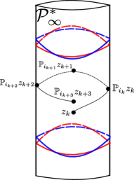
Figure 3.2. The invariant curves of the map $\mathbb{P}_{+}$ (in red) intersect transversally the invariant curves of the map $\mathbb{P}_{-}$ (in blue). We also sketch a segment of a diffusive orbit for the iterated function system generated by the maps $\mathbb{P}_{\pm}$.

3.6. Shadowing and existence of a transition chain

We now consider the iterated function system generated by the maps $\mathbb{P}_{\pm}$. Since the maps $\mathbb{P}_{\pm}$ are both twist maps and share no common invariant curve on $\mathcal{P}_{\infty}^{*}$ , it is proven in [Moe02] (see also [LC07]) that the iterated function system generated by the maps $\mathbb{P}_{\pm}$ possesses drift orbits in $\mathcal{P}^{*}_{\infty}$.

Theorem 3.14.

Let $\mathbb{P}_{\pm}$ be the maps defined in (3.23). Then, there exists $I_{*}$ such that, for any $\epsilon\in(0,I_{*}^{-3})$ and any pair $I_{1},I_{2}$ satisfying

$$I_{*}\leq I_{1}\leq I_{2}\leq\epsilon^{-1/3},$$

there exists $N\in\mathbb{N}$ and a sequence

$$\{(i_{k},z_{k})\}_{1\leq k\leq N}\subset\left(\{+,-\}\times\mathcal{P}_{\infty}^{*}\right)^{N}\qquad\qquad z_{k+1}=\mathbb{P}_{i_{k}}(z_{k})$$

such that

$$\pi_{I}z_{1}\leq I_{1}\qquad\qquad\text{and}\qquad\qquad I_{2}\leq\pi_{I}z_{N}.$$

Finally, the proof of Theorem 1.1 is completed by standard shadowing results (see Figure 3.3). Let $(\varphi,I)\in\mathcal{P}_{\infty}^{*}$, which is a parabolic fixed point of the Poincaré map $P$ in (3.17) and denote by $W_{\varphi,I}^{\mathrm{u},\mathrm{s}}$ its stable and unstable manifolds. For a number $\delta>0$ and a point $p\in\{t=0\}$ and denote by $B_{\delta}(p)\subset\{t=0\}$ the ball of radius $\delta$ centered at $p$ at the Poincaré section. The following shadowing result for TNHIC, proved in [GSMS17] fits our purposes.

Proposition 3.15 (Proposition 2 in [GSMS17]).

Let $N\in\mathbb{N}\cup\{\infty\}$ and let $\{(\varphi_{k},I_{k})\}_{1\leq k\leq N}$ be a family of fixed points in $\mathcal{P}_{\infty}^{*}$ for the Poincaré map $P$ such that, for all $1\leq k\leq N$, $W^{\mathrm{u}}_{\varphi_{k},I_{k}}$ intersects transversally $W^{\mathrm{s}}(\mathcal{P}_{\infty}^{*})$ at a point $p_{k}\in W^{s}_{\varphi_{k+1},I_{k+1}}$. Then, for any sequence $\{\delta_{k}\}_{k\geq 1}$ with $\delta_{k}>0$ there exists a point $z\in B_{\delta_{1}}(\varphi_{0},I_{0})$ and two sequences $\{n_{k}\}_{1\leq k\leq N},\{\tilde{n}_{k}\}_{1\leq k\leq N},\subset\mathbb{N}$ with $n_{k}<\tilde{n}_{k}<n_{k+1}<\tilde{n}_{k+1}$ such that $P^{n_{k}}(z)\in B_{\delta_{k}}(\varphi_{k},I_{k})$ and $P^{\tilde{n}_{k}}(z)\in B_{\delta_{k}}(p_{k})$ for all $1\leq k\leq N$.

Let $\{z_{k}\}_{1\leq k\leq N}=\{(\varphi_{k},I_{k})\}_{1\leq k\leq N}\subset\mathcal{P}_{\infty}^{*}$ be the sequence of fixed points for the Poincaré map $P$ given in Theorem 3.14 and apply Proposition 3.15 with $\delta_{k}>0$ small enough. The proof of Theorem 1.1 is complete.

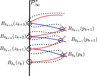
Figure 3.3. A true orbit of the RPE3BP which shadows the pseudo orbit $\{z_{k}\}_{1\leq k\leq N}$ obtained in Theorem 3.14. In blue (red) we skecth segments of the stable (unstable) manifolds associated to parabolic fixed points $\{z_{k}\}_{0\leq k\leq N}$ of the Poincaré map $P$.

4. The generating functions of the invariant manifolds

In this section we provide the proof of Propositions 3.2 and 3.3 and show how the latter readily implies Theorem 3.4. First we show the existence of real analytic solutions $T^{\mathrm{u,s}}(u,\beta,t;I^{\mathrm{u}},I^{\mathrm{s}},\epsilon)$ to the Hamilton-Jacobi equation associated to the Hamiltonian $H$ in (3.6). That is,

$$H(q,\delta^{\mathrm{u},\mathrm{s}}+\nabla T^{\mathrm{u},\mathrm{s}}(q))=0\qquad\qquad q=(u,v,t)$$

with $\delta^{\mathrm{u}}=(0,(I^{\mathrm{u}}-I^{\mathrm{s}})/2,0)$, $\delta^{s}=(0,(I^{\mathrm{s}}-I^{\mathrm{u}})/2,0)$ and asymptotic conditions

$$\lim_{\mathrm{Re}u\to-\infty}T^{\mathrm{u}}(u,\beta,t;I^{\mathrm{u}},I^{\mathrm{s}},\epsilon)=0\qquad\qquad\lim_{\mathrm{Re}u\to\infty}T^{s}(u,\beta,t;I^{\mathrm{u}},I^{\mathrm{s}},\epsilon)=0$$

on certain complex domains of the form $D^{\mathrm{u},\mathrm{s}}\times\mathbb{T}^{2}$ defined below, which satisfy

$$D^{\mathrm{u}}\cap D^{s}\neq\emptyset,\qquad\qquad\text{and}\qquad\qquad\left((-\infty,-u_{0}]\cup[u_{1},u_{2}]\right)\times\mathbb{T}^{2}\subset D^{\mathrm{u}}\times\mathbb{T}^{2},\qquad[u_{0},\infty)\times\mathbb{T}^{2}\subset D^{s}\times\mathbb{T}^{2}$$

for some real values $u_{0}<u_{1}<u_{2}$. This is the content of Sections 4.2 and 4.3. Then, in Section 4.4 we study the difference

$$\Delta S(q;I^{\mathrm{u}},I^{\mathrm{s}},\epsilon)=\langle\delta^{\mathrm{u}}-\delta^{\mathrm{s}},q\rangle+(T^{\mathrm{u}}-T^{\mathrm{s}})(q;I^{\mathrm{u}},I^{\mathrm{s}},\epsilon)$$

on the complex domain $(D^{\mathrm{u}}\cap D^{\mathrm{s}})\times\mathbb{T}^{2}$ and show that $\Delta S$ is approximated uniformly in $(D^{\mathrm{u}}\cap D^{\mathrm{s}})\times\mathbb{T}^{2}$ by

$$\Delta S\sim\langle\delta^{\mathrm{u}}-\delta^{\mathrm{s}},q\rangle+\tilde{L}$$

where $\tilde{L}$ is the Melnikov potential (recall that $I_{\mathrm{m}}=(I^{\mathrm{u}}+I^{\mathrm{s}})/2$) defined by

(4.1) $$\tilde{L}(u,\beta,t;I_{\mathrm{m}},\epsilon)=\int_{\mathbb{R}}V(s,\beta,t-I_{\mathrm{m}}^{3}u+I_{\mathrm{m}}^{3}s;I_{\mathrm{m}},\epsilon)\mathrm{d}s.$$

Remark 16.

The function $\tilde{L}$ satisfies

$$\tilde{L}(u,\beta,t;I_{\mathrm{m}},\epsilon)=L(t-I_{\mathrm{m}}^{3}u,\beta;I_{\mathrm{m}},\epsilon)$$

where $L(\sigma,\beta;I_{\mathrm{m}},\epsilon)$ was defined in (3.15). The introduction of (4.1) is just a matter of convenience for the forthcoming sections.

Finally, we prove that the existence of nondegenerate critical points of the function

$$q\mapsto\langle\delta^{\mathrm{u}}-\delta^{\mathrm{s}},q\rangle+\tilde{L}(q;I^{\mathrm{u}},I^{\mathrm{s}},\epsilon)$$

implies the existence of nondegenerate critical points of the function $q\mapsto\Delta S(q;I^{\mathrm{u}},I^{\mathrm{s}},\epsilon)$.

4.1. From the circular to the elliptic problem

As pointed out in the introduction, for $\epsilon=0$ and $\mu>0$, which corresponds to the circular problem (RPC3BP), the system is already non integrable since there exist transverse intersections between the stable and unstable manifolds of all the tori $\mathcal{T}_{I}\subset\mathcal{P}_{\infty}$ with $I$ sufficiently large (see [GMS16]). However, for $\epsilon=0$, due to the conservation of the Jacobi constant, there do not exist heteroclinic connections between different tori $\mathcal{T}_{I},\mathcal{T}_{I^{\prime}}\subset\mathcal{P}_{\infty}$. In Theorem 3.4 we prove that for $\epsilon>0$ there do exist heteroclinic connections between sufficiently close $\mathcal{T}_{I},\mathcal{T}_{I^{\prime}}\subset\mathcal{P}_{\infty}$. As explained at the beginning of Section 4 this result will be proved by approximating the difference $\Delta S$ by the Melnikov potential $L$. In this approximation there are errors errors coming from the circular part of the perturbation and errors exclusive of the elliptic part. For this reason, in order to obtain asymptotic formulas for the scattering maps associated to the aforementioned heteroclinic intersections, in the case $\mu,\epsilon>0$, it is necessary to keep track of the $\epsilon$ dependent part in the generating functions $T^{\mathrm{u,s}}$. To that end, we denote by (see [GMS16])

(4.2) $$T_{\mathrm{circ}}^{\mathrm{u,s}}(u,t-\beta;I_{\mathrm{m}})=T^{\mathrm{u,s}}(u,\beta,t;I_{\mathrm{m}},I_{\mathrm{m}},0),$$

the generating functions associated to the invariant manifolds of the invariant torus $\mathcal{T}_{I_{\mathrm{m}}}\subset\mathcal{P}_{\infty}$ for the circular problem ($\epsilon=0$), let

(4.3) $$V_{\mathrm{circ}}(u,t-\beta;I_{\mathrm{m}})=V(u,\beta,t;I_{\mathrm{m}},0)$$

and introduce the Melnikov potential associated to the circular problem

(4.4) $$\tilde{L}_{\mathrm{circ}}(u,t-\beta;I_{\mathrm{m}})=\tilde{L}(u,\beta,t;I_{\mathrm{m}},0).$$

4.2. Analytic continuation of the unstable generating function

Consider the domain (see Figure 4.1 and Remark 8)

(4.5) $$D^{\mathrm{u}}_{\kappa}=\{u\in\mathbb{C}\colon|\mathrm{Im}u|\leq 1/3-\kappa|I_{\mathrm{m}}|^{-3}-\tan\beta_{1}\mathrm{Re}u,\ |\mathrm{Im}u|\geq 1/6+\kappa|I_{\mathrm{m}}|^{-3}-\tan\beta_{2}\mathrm{Re}u\},$$

where $\beta_{1},\beta_{2}\in(0,\pi/2)$, $\beta_{1}<\beta_{2}$ and $\kappa>0$ is a given constant. It is clear that for $I_{\mathrm{m}}$ large enough $D^{\mathrm{u}}_{\kappa}$ is non empty. The role of the parameter $\kappa$ is to shrink the domain $D^{\mathrm{u}}_{\kappa}$ when, in Sections 4.3 and 4.4, we introduce close to identity changes of variables and make use of Cauchy estimates.

In this section we prove the existence of positive constants $\kappa,\rho$ and $\sigma$ such that for all $I_{*}$ large enough and any $I_{\mathrm{m}}\in\Lambda_{\rho,I}(I_{*})$, $|I^{\mathrm{u}}-I^{\mathrm{s}}|\leq\epsilon|I_{\mathrm{m}}|^{-4}$, where $\Lambda_{\rho,I}$ is introduced in (3.3), there exists a unique real analytic solution to the Hamilton-Jacobi equation

(4.6) $$H(q,\delta^{\mathrm{u}}+\nabla T^{\mathrm{u}})=(1+A^{\mathrm{u}}(q,\delta^{\mathrm{u}}+\nabla T^{\mathrm{u}}))\partial_{u}T^{\mathrm{u}}+B^{\mathrm{u}}(q,\delta^{\mathrm{u}}+\nabla T^{\mathrm{u}})\partial_{\beta}T^{\mathrm{u}}+I_{\mathrm{m}}^{3}\partial_{t}T^{\mathrm{u}}-V(q)=0$$

with asymptotic condition $\lim_{\mathrm{Re}u\to-\infty}T^{\mathrm{u}}=0$ in the complex domain $(u,\beta,t)\in D^{\mathrm{u}}_{\kappa}\times\mathbb{T}_{\rho}\times\mathbb{T}_{\sigma}$ and where

(4.7) $$A^{\mathrm{u}}=\frac{1}{2y_{\mathrm{h}}^{2}I_{\mathrm{m}}}\left(\partial_{u}T^{\mathrm{u}}-r_{\mathrm{h}}^{-2}(\delta^{\mathrm{u}}+\partial_{\beta}T^{\mathrm{u}})\right)\qquad\qquad B^{\mathrm{u}}=-\frac{1}{2y_{\mathrm{h}}^{2}r_{\mathrm{h}}^{2}I_{\mathrm{m}}}\left(\partial_{u}T^{\mathrm{u}}-r_{\mathrm{h}}^{-1}(\delta^{\mathrm{u}}+\partial_{\beta}S^{\mathrm{u}}\right).$$

The existence of $T^{\mathrm{s}}$ solving the corresponding Hamilton-Jacobi equation on $D^{\mathrm{s}}\times\mathbb{T}_{\rho}\times\mathbb{T}_{\sigma}$ with $D^{s}_{\kappa}=\{u\in\mathbb{C}\colon-u\in D^{\mathrm{u}}_{\kappa}\}$ is obtained by a completely analogous argument.

Figure 4.1. The complex domains $D^{\mathrm{u}}_{\kappa}$ and $D^{\mathrm{s}}_{\kappa}$.

Remark 17.

The use of different widths for the strips in the angles $\beta$ and $t$ is only a technical issue. The solution to the Hamilton-Jacobi equation (4.6) will be obtained by means of a Newton method in which the size of the strip $\mathbb{T}_{\rho}$ for the angle $\beta$ is reduced at each iteration while the size of the strip $\mathbb{T}_{\sigma}$ for the $t$ variable can be kept constant. For this reason, in all the forthcoming notation, we omit the dependence on $\sigma$ and only emphasize the dependence on $\rho$.

The width of the strip of analyticity in the angle $\beta$ is taken to be the same than the width of the complex neighborhood for the parameter $I_{\mathrm{m}}$. This is an arbitrary choice to avoid introducing more notation.

Let $\eta,\nu$ be positive real constants. We now introduce the family of Banach spaces of sequences of analytic functions in which we will look for solutions to (4.6)

(4.8) $$\mathcal{Z}_{\eta,\nu,\rho}=\left\{h=\{h^{[l]}\}_{l\in\mathbb{Z}}\colon\ h^{[l]}:D^{\mathrm{u}}_{\kappa}\times\mathbb{T}_{\rho}\to\mathbb{C}\ \text{is analytic for all }l\in\mathbb{Z}\ \text{and}\ \lVert h\rVert_{\eta,\nu,\rho}<\infty\right\}$$

where $\lVert\cdot\rVert_{\eta,\nu,\rho}$ is the Fourier sup norm

$$\lVert h\rVert_{\eta,\nu,\rho}=\sum_{l\in\mathbb{Z}}\lVert h^{[l]}\rVert_{\eta,\nu,\rho,l}e^{|l|\sigma}$$

defined by

$$\begin{split}\lVert h\rVert_{\eta,\nu,\rho,l}=&\sup_{(u,\beta)\in(D^{\mathrm{u}}_{\kappa}\cap\{\mathrm{Re}(u)\leq-1\})\times\mathbb{T}_{\rho}}\left|u^{\eta}h^{[l]}(u,\beta)\right|\\ &+\sup_{(u,\beta)\in(D^{\mathrm{u}}_{\kappa}\cap\{\mathrm{Re}(u)\geq-2\})\times\mathbb{T}_{\rho}}\left|(u-i/3)^{\nu+l/2}(u+i/3)^{\nu-l/2}h^{[l]}(u,\beta)\right|.\end{split}$$

It will also be convenient for us to introduce the Banach spaces

(4.9) $$\mathcal{X}_{\eta,\nu,\rho}=\left\{h=\{h^{[l]}\}_{l\in\mathbb{Z}}\ \colon\ h^{[l]}:D^{\mathrm{u}}_{\kappa}\times\mathbb{T}_{\rho}\to\mathbb{C}\ \text{is analytic for all }l\in\mathbb{Z}\ \text{and}\ \llbracket h\rrbracket_{\eta,\nu,\rho}<\infty\right\}.$$

where

(4.10) $$\llbracket h\rrbracket_{\eta,\nu,\rho}=\lVert h\rVert_{\eta,\nu,\rho}+\lVert\partial_{u}h\rVert_{\eta+1,\nu+1,\rho}.$$

Remark 18.

It is straightforward to check that the elements of $\mathcal{Z}_{\eta,\nu,\rho}$ and $\mathcal{X}_{\eta,\nu,\rho}$ can be identified with Fourier series

$$h(u,\beta,t)=\sum_{l\in\mathbb{Z}}h^{[l]}(u,\beta)e^{ilt}$$

which, for a given $u\in D^{\mathrm{u}}$, converge on the strip

$$\mathbb{T}_{\sigma}(u)=\left\{t\in\mathbb{C}/2\pi\mathbb{Z}\colon\left|\mathrm{Im}(t)-\frac{1}{2}\left(\ln(|u-i/3|)-\ln(|u+i/3|)\right)\right|\leq\sigma\right\}.$$

That is, they yield well defined functions for $(u,\beta)\in D^{\mathrm{u}}_{\kappa}\times\mathbb{T}_{\rho}$ and $t\in\mathbb{T}_{\sigma}(u)$. Alternatively one can think of the elements of $\mathcal{X}_{\eta,\nu,\rho}$ as formal Fourier series on the strip $\mathbb{T}_{\sigma}$ (see [GMS16] and [GMPS22]).

Remark 19.

In the case $I^{\mathrm{u}},I^{\mathrm{s}}\in\mathbb{R}$, one can replace analytic by real analytic in the definition of $\mathcal{Z}_{\eta,\nu,\rho}$ and $\mathcal{X}_{\eta,\nu,\rho}$.

In the following lemma we list some properties of the spaces $\mathcal{X}_{\eta,\nu,\rho}$ which will be useful. The proof is straightforward.

Lemma 4.1.

The following statements hold:

• (Graded algebra property) For any $g\in\mathcal{X}_{\eta,\nu,\rho}$ and $f\in\mathcal{X}_{\eta^{\prime},\nu^{\prime},\rho}$, their product satisfies $gf\in\mathcal{X}_{\eta+\eta^{\prime},\nu+\nu^{\prime},\rho}$.

• Let $h\in\mathcal{X}_{\eta,\nu,\rho}$. Then, for $\eta^{\prime}<\eta$ and $\nu^{\prime}<\nu$ we have $h\in\mathcal{X}_{\eta^{\prime},\nu^{\prime},\rho}$ and

  $$\lVert h\rVert_{\eta^{\prime},\nu^{\prime},\rho}\leq|I_{\mathrm{m}}|^{3(\nu-\nu^{\prime})}\lVert h\rVert_{\eta,\nu,\rho}$$

• Let $h\in\mathcal{X}_{\eta,\nu,\rho}$. Then for any $0<\delta<\rho$ we have that $\partial_{\beta}h\in\mathcal{X}_{\eta,\nu,\rho-\delta}$ and

  $$\lVert\partial_{\beta}h\rVert_{\eta,\nu,\rho-\delta}\leq\delta^{-1}\lVert h\rVert_{\eta,\nu,\rho}.$$

We also state the following lemma, which will be useful to deal with compositions in the angular variable $\beta$. The proof can be found in [GMS16].

Lemma 4.2.

Let $h\in\mathcal{X}_{\eta,\nu,\rho}$ and let $g_{i}\in\mathcal{X}_{0,0,\rho^{\prime}}$ with $\rho>\rho^{\prime}$, $i=1,2,$ and

$$\lVert g_{i}\rVert_{0,0,\rho^{\prime}}\leq\frac{\rho-\rho^{\prime}}{2}.$$

Write $h\circ(\mathrm{Id}+g_{i})(u,\beta,t)=h(u,\beta+g_{i}(u,\beta,t),t)$. Then, $h\circ(\mathrm{Id}+g_{i})\in\mathcal{X}_{\eta,\nu,\rho^{\prime}}$ with

$$\lVert h\circ(\mathrm{Id}+g_{i})\rVert_{\eta,\nu,\rho^{\prime}}\lesssim\lVert h\rVert_{\eta,\nu,\rho}.$$

Moreover, for $f=h\circ(\mathrm{Id}+g_{2})-h\circ(\mathrm{Id}+g_{1})$ we have

$$\lVert f\rVert_{\eta,\nu,\rho^{\prime}}\lesssim(\rho-\rho^{\prime})^{-1}\lVert h\rVert_{\eta,\nu,\rho}\lVert g_{2}-g_{1}\rVert_{0,0,\rho^{\prime}}.$$

The choice of the functional space for solving (4.6) is motivated by the following result proved in Appendix A.

Lemma 4.3.

Fix $\kappa>0$ and $\sigma>0$. Then, there exist $\rho_{0},I_{*}>0$ such that, for $\epsilon\in(0,I_{*}^{-3})$, and $I^{\mathrm{u}},I^{\mathrm{s}}$ with $I_{\mathrm{m}}\in\Lambda_{\rho_{0},I}$, the perturbative potential $V(v,\beta,t;I_{\mathrm{m}})$ defined in (3.7) satisfies $V\in\mathcal{X}_{2,3/2,\rho_{0}}$. Moreover

$$\lVert V\rVert_{2,3/2,\rho_{0}}\lesssim|I_{\mathrm{m}}|^{-3}$$

and

$$\lVert V-V_{\mathrm{circ}}\rVert_{2,3/2,\rho_{0}}\lesssim\epsilon|I_{\mathrm{m}}|^{-3}$$

where $V_{\mathrm{circ}}$ was defined in (4.3).

We now state the main result in this section.

Theorem 4.4.

Let $\kappa,\sigma>0$ and $\rho_{0}>0$ as in Lemma 4.3. Then, there exist $\rho\in(0,\rho_{0})$ and $I_{*}>0$ such that for for $\epsilon\in(0,I_{*}^{-3})$, and $I^{\mathrm{u}},I^{\mathrm{s}}$ such that $I_{\mathrm{m}}=(I^{\mathrm{u}}+I^{\mathrm{s}})/2\in\Lambda_{\rho,I}(I_{*})$, and $|I^{\mathrm{u}}-I^{\mathrm{s}}|\leq\epsilon|I_{\mathrm{m}}|^{-4}$, there exists $T^{\mathrm{u}}\in\mathcal{X}_{1/3,1/2,\rho}$ solution to the Hamilton-Jacobi equation (4.6) such that

$$\lVert T^{\mathrm{u}}\rVert_{1/3,1/2,\rho}\lesssim|I_{\mathrm{m}}|^{-3}\qquad\qquad\text{and}\qquad\qquad\lVert T^{\mathrm{u}}-L^{\mathrm{u}}\rVert_{1/3,1,\rho}\lesssim|I_{\mathrm{m}}|^{-7},$$

where $L^{\mathrm{u}}$ is the unstable half Melnikov potential

(4.11) $$L^{\mathrm{u}}(u,\beta,t;I_{\mathrm{m}},\epsilon)=\int_{-\infty}^{0}V(u+s,\beta,t+I_{\mathrm{m}}^{3}s;I_{\mathrm{m}},\epsilon)\mathrm{d}s.$$

Moreover,

$$\lVert T^{\mathrm{u}}-T^{\mathrm{u}}_{\mathrm{circ}}-(L^{\mathrm{u}}-L^{\mathrm{u}}_{\mathrm{circ}})\rVert_{1/3,1,\rho}\lesssim\epsilon|I_{\mathrm{m}}|^{-7},$$

where $T^{\mathrm{u}}_{\mathrm{circ}}$ is defined in (4.2) and $L^{\mathrm{u}}_{\mathrm{circ}}(u,t-\beta;I_{\mathrm{m}})=L^{\mathrm{u}}(u,\beta,t;I_{\mathrm{m}},0)$.

The proof of Theorem 4.4 will be accomplished by a Newton iterative scheme. That is, we obtain $T^{\mathrm{u}}$ as the limit of an iterative process $T^{\mathrm{u}}=\lim_{n\to\infty}T_{n}$ where $T_{0}=0$ and the $n$-th step is obtained as the solution to the linear equation

(4.12) $$H(T_{n-1})+DH(T_{n-1})[T_{n}-T_{n-1}]=0$$

where, by abuse of notation we have written (and will write in the forthcoming sections)

$$H(T_{n})=H(q,\delta^{\mathrm{u}}+\nabla T_{n};I^{\mathrm{u}},I^{\mathrm{s}})$$

and $H$ is given in (3.6). One can check that the linearized operator $DH(T)[\cdot]$ reads

(4.13) $$\begin{split}DH(T)[\cdot]=&\left(1+y_{\mathrm{h}}^{-2}I_{\mathrm{m}}^{-1}\left(\partial_{u}T-r_{\mathrm{h}}^{-2}(\delta^{\mathrm{u}}_{\beta}+\partial_{\beta}T)\right)\right)\partial_{u}[\cdot]\\ &-y_{\mathrm{h}}^{-2}r_{\mathrm{h}}^{-2}I_{\mathrm{m}}^{-1}\left(\partial_{u}T-2r_{\mathrm{h}}^{-1}(\delta^{\mathrm{u}}_{\beta}+\partial_{\beta}T)\right)\partial_{\beta}[\cdot]+I_{\mathrm{m}}^{3}\partial_{t}[\cdot],\end{split}$$

where we recall that

$$\delta^{\mathrm{u}}_{\beta}=\frac{1}{2}(I^{\mathrm{u}}-I^{\mathrm{s}}).$$

Since $H$ is quadratic in $\nabla T$ the second differential of $H$ is a bilinear operator and the error we accomplish at the step $n$ is

(4.14) $$H(T_{n})=D^{2}H\left[\Delta T_{n},\Delta T_{n}\right]=y_{\mathrm{h}}^{-2}I_{\mathrm{m}}^{-1}\left(\left(\partial_{u}\Delta T_{n}\right)^{2}-2r_{\mathrm{h}}^{-2}\partial_{u}\Delta T_{n}\partial_{\beta}\Delta T_{n}+2r_{\mathrm{h}}^{-1}\left(\partial_{\beta}\Delta T_{n}\right)^{2}\right)$$

where we have introduced the notation $\Delta T_{n}=T_{n}-T_{n-1}$.

In the proof of Theorem 4.4 we treat $DH(T)[\cdot]$ as a small perturbation of the constant coefficients linear operator

(4.15) $$\mathcal{L}[\cdot]=(\partial_{u}+I_{\mathrm{m}}^{3}\partial_{t})[\cdot].$$

The next technical lemma, proved in [GOS10], shows the existence of a right inverse for $\mathcal{L}$ on the functional space $\mathcal{X}_{\eta,\nu,\rho}$ with $\eta>1$.

Lemma 4.5.

Let $\mathcal{L}$ be the operator defined in (4.15). Then, for any $\eta>1$ there exists an operator $\mathcal{G}:\mathcal{X}_{\eta,\nu,\rho}\to\mathcal{X}_{\eta-1,\nu,\rho}$, given by

(4.16) $$\mathcal{G}(h)(u,\beta,t)=\int_{-\infty}^{0}h(u+s,\beta,t+I_{\mathrm{m}}^{3}s)\mathrm{d}s,$$

such that $\mathcal{L}\circ\mathcal{G}=\mathrm{Id}:\mathcal{X}_{\eta,\nu,\rho}\to\mathcal{X}_{\eta,\nu,\rho}$. Moreover, for any $h\in\mathcal{X}_{\eta,\nu,\rho}$ with $\eta,\nu>1$ the following estimates hold

$$\lVert\mathcal{G}(h)\rVert_{\eta-1,\nu-1,\rho}\lesssim\lVert h\rVert_{\eta,\nu,\rho}\qquad\qquad\text{and}\qquad\qquad\lVert\partial_{u}\mathcal{G}(h)\rVert_{\eta,\nu,\rho}\lesssim\lVert h\rVert_{\eta,\nu,\rho}.$$

Remark 20.

Lemma 4.5 or similar versions are usually proved for $I_{\mathrm{m}}\in\mathbb{R}$ (see [GOS10]). As for $I_{\mathrm{m}}\in\Lambda_{\rho,I}$ we have

$$\arg(I_{\mathrm{m}})=\tan^{-1}(\mathcal{O}(|I_{\mathrm{m}}|^{-1}))=\mathcal{O}(|I_{\mathrm{m}}|^{-1}),$$

and it is straightforward to check that the same proof applies for $I_{\mathrm{m}}\in\Lambda_{\rho,I}$.

4.2.1. First step of the Newton scheme

The iterative scheme proposed above defines the function $T_{1}$ as the solution to the linearized equation

(4.17) $$H(0)+DH(0)[T_{1}]=0.$$

Instead, it will be convenient to modify the first step of the iterative process and define $T_{1}$ as the solution to

(4.18) $$\mathcal{L}T_{1}=-H(0),$$

where $\mathcal{L}$ is the constant coefficients linear operator defined in (4.15). Using Lemma 4.5 we can rewrite (4.17) as

(4.19) $$T_{1}=-\mathcal{G}(H(0)).$$

The properties of the unperturbed homoclinic stated in Lemma 2.1, Lemma 4.3 for the potential $V$ and the hypothesis $|\delta^{\mathrm{u}}_{\beta}|\lesssim\epsilon|I_{\mathrm{m}}|^{-4}$ imply that (here $\rho_{0}$ is the constant given in Lemma 4.3)

(4.20) $$\lVert H(0)\rVert_{4/3,3/2,\rho_{0}}=\lVert y_{\mathrm{h}}^{-2}r_{\mathrm{h}}^{-3}I_{\mathrm{m}}^{-1}(\delta^{\mathrm{u}}_{\beta})^{2}-V\rVert_{4/3,3/2,\rho_{0}}\lesssim|I_{\mathrm{m}}|^{-3}\equiv\varepsilon_{0}.$$

Therefore, it follows from Lemma 4.5 that $T_{1}\in\mathcal{X}_{1/3,1/2,\rho_{0}}$ with

(4.21) $$\llbracket T_{1}\rrbracket_{1/3,1/2,\rho_{0}}\lesssim\varepsilon_{0}.$$

The error in this first approximation is given by

$$H(T_{1})=D^{2}H[T_{1},T_{1}]+\left(DH(T_{1})-\mathcal{L}\right)[T_{1}].$$

Using Lemma 2.1, Lemma 4.1, and the expressions (4.13) and (4.14), we obtain that for $0<\delta_{0}<\rho_{0}$

$$\begin{split}\lVert D^{2}H[T_{1},T_{1}]\rVert_{4/3,3/2,\rho_{0}-\delta_{0}}\lesssim|I_{\mathrm{m}}|^{1/2}&\left(\lVert\partial_{u}T_{1}\rVert^{2}_{4/3,3/2,\rho_{0}}+\lVert\partial_{u}T_{1}\rVert_{4/3,3/2,\rho_{0}}\lVert\partial_{\beta}T_{1}\rVert_{1/3,1/2,\rho_{0}-\delta_{0}}\right.\\ +&\left.|I_{\mathrm{m}}|^{-3/2}\lVert\partial_{\beta}T_{1}\rVert^{2}_{4/3,3/2,\rho_{0}-\delta_{0}}\right)\end{split}$$

and

$$\lVert\left(DH(T_{1})-\mathcal{L}\right)[T_{1}]\rVert_{4/,3/2,\rho_{0}-\delta_{0}}\lesssim|I_{\mathrm{m}}|^{-1}|\delta^{\mathrm{u}}_{\beta}|\left(\lVert\partial_{u}T_{1}\rVert_{1/3,1/2,\rho_{0}-\delta_{0}}+\lVert\partial_{\beta}T_{1}\rVert_{1/3,1/2,\rho_{0}-\delta_{0}}\right).$$

Then, it follows from the estimate (4.21) for $T_{1}$, the hypothesis $|\delta^{\mathrm{u}}_{\beta}|\lesssim\epsilon|I_{\mathrm{m}}|^{-4}$ and the third and fourth items in Lemma 4.1, that

$$\lVert H(T_{1})\rVert_{4/3,3/2,\rho_{0}-\delta_{0}}\lesssim|I_{\mathrm{m}}|^{1/2}\varepsilon_{0}^{2}\left(1+\delta_{0}^{-1}+I_{\mathrm{m}}^{-3/2}\delta_{0}^{-2}\right)\lesssim|I_{\mathrm{m}}|^{1/2}\varepsilon_{0}^{2}\delta_{0}^{-2},$$

where $\varepsilon_{0}$ was defined in (4.20). We now take

$$\delta_{0}\equiv\varepsilon_{0}^{1/8}\qquad\text{and define}\qquad\rho_{1}=\rho_{0}-\delta_{0}.$$

Therefore,

$$\lVert H(T_{1})\rVert_{4/3,3/2,\rho_{1}}\lesssim|I_{\mathrm{m}}|^{1/2}\varepsilon_{0}^{1/4}\varepsilon_{0}^{3/2}\leq\varepsilon_{0}^{3/2}\equiv\varepsilon_{1}.$$

4.2.2. The iterative argument

Throughout this section, the symbol $a\lesssim b$ means that there exists $C>0$ which does not depend on the step $n$ and $I_{\mathrm{m}}$ such that $a\leq Cb$.

Through the Newton iteration scheme, at the step $n+1$, we have to solve the linearized equation

$$H(T_{n})+DH(T_{n})[\varDelta T_{n+1}]=0\qquad\qquad\varDelta T_{n+1}=T_{n+1}-T_{n}.$$

For that, we have to invert the linear operator $DH(T_{n})[\cdot]$ defined in (4.13). Since this operator has a non zero coefficient multiplying $\partial_{\beta}$ we must find a change of variables

(4.22) $$(u,\beta,t)=\Psi_{n+1}(u,\varphi,t)\equiv(u,\varphi+\psi_{n+1}(u,\varphi,t),t),$$

in which the linearized operator does not involve partial derivatives with respect to the new angle $\varphi$. Define

(4.23) $$A_{n}=\frac{1}{2y_{\mathrm{h}}^{2}I_{\mathrm{m}}}\left(\partial_{u}T_{n}-r_{\mathrm{h}}^{-2}(\delta^{\mathrm{u}}_{\beta}+\partial_{\beta}T_{n})\right)\qquad\qquad B_{n}=-\frac{1}{2y_{\mathrm{h}}^{2}r_{\mathrm{h}}^{2}I_{\mathrm{m}}}\left(\partial_{u}T_{n}-r_{\mathrm{h}}^{-1}(\delta^{\mathrm{u}}_{\beta}+\partial_{\beta}T_{n})\right).$$

Then, one can check that, if one considers a change of variables (4.22) with $\psi_{n+1}$ solving (here $\mathcal{L}$ is the operator (4.15))

$$\mathcal{L}\psi_{n+1}=B_{n}\circ\Psi_{n+1}-(A_{n}\circ\Psi_{n+1})\partial_{v}\psi_{n+1},$$

the following equations determining an unknown function $h$ are equivalent

(4.24) $$DH(T_{n})[h]+H(T_{n})=0\quad\quad\Longleftrightarrow\quad\quad(1+A_{n}\circ\Psi_{n+1})\partial_{u}(h\circ\Psi_{n+1})+I_{\mathrm{m}}^{3}\partial_{t}(h\circ\Psi_{n+1})+H(T_{n})\circ\Psi_{n+1}=0.$$

Indeed, if we denote by $\Delta\widetilde{T}_{n+1}$ the solution of the second equation in (4.24), then

$$\Delta T_{n+1}=\Delta\widetilde{T}_{n+1}\circ\Psi_{n+1}^{-1}$$

solves the first equation in (4.24). As a consequence, we define

$$T_{n+1}=T_{n}+\Delta\widetilde{T}_{n+1}\circ\Psi_{n+1}^{-1}$$

and

$$\widetilde{T}_{n+1}=T_{n+1}\circ\Psi_{n+1}=\widetilde{T}_{n}\circ\Psi_{n}^{-1}\circ\Psi_{n+1}+\Delta\tilde{T}_{n+1}.$$

In order to state the inductive hypothesis, we define now the constants

(4.25) $$\varepsilon_{n}=\varepsilon_{n-1}^{3/2}\qquad\qquad\delta_{n}=\varepsilon_{n}^{1/8}\qquad\qquad\rho_{n}=\rho_{n-1}-2\delta_{n-1}.$$

Notice that it follows (taking $\varepsilon_{0}$ small enough) from this definition that $\rho_{n}\geq\rho_{0}/2\ \ \forall n\in\mathbb{N}\cup\{\infty\}$. Suppose that:

• (H1) There exists a family of functions $\{\widetilde{T}_{i}\}_{1\leq i\leq n}\subset\mathcal{X}_{1/3,1/2,\rho_{i-1}}$ and a family of close to identity maps $\Psi_{1}=\mathrm{Id}$ and $\left\{\Psi_{i}\right\}_{2\leq i\leq n}$ with $\Psi_{i}=\mathrm{Id}+\psi_{i}$, $\psi_{i}\in\mathcal{X}_{2/3,1/2,\rho_{i-1}}$, such that

  $$\mathcal{L}\psi_{i+1}=B_{i}\circ\Psi_{i+1}-(A_{i}\circ\Psi_{i+1})\partial_{u}\psi_{i+1},$$

  where now $A_{i},B_{i}$ are written in terms of $\tilde{T}_{i}$

  $$\begin{split}A_{i}=&\frac{1}{2y_{\mathrm{h}}^{2}I_{\mathrm{m}}}\left(\partial_{u}(\widetilde{T}_{i}\circ\Psi_{i}^{-1})-r_{\mathrm{h}}^{-2}(\delta^{\mathrm{u}}_{\beta}+\partial_{\beta}(\widetilde{T}_{i}\circ\Psi_{i}^{-1}))\right)\\ B_{i}=&-\frac{1}{2y_{\mathrm{h}}^{2}r_{\mathrm{h}}^{2}I_{\mathrm{m}}}\left(\partial_{u}(\widetilde{T}_{i}\circ\Psi_{i}^{-1})-r_{\mathrm{h}}^{-1}(\delta^{\mathrm{u}}_{\beta}+\partial_{\beta}(\widetilde{T}_{i}\circ\Psi_{i}^{-1}))\right).\\ \end{split}$$

• (H2) The functions $\psi_{i}$ satisfy (see Remark 21 below)

  $$\llbracket\psi_{i+1}-\psi_{i}\rrbracket_{2/3,1/2,\rho_{i}}\lesssim|I_{\mathrm{m}}|^{-1}\delta_{i-1}^{7}.$$

• (H3) The functions $\widetilde{T}_{i}$ satisfy

  $$\llbracket\widetilde{T}_{i+1}-\widetilde{T}_{i}\circ\Psi_{i}^{-1}\circ\Psi_{i+1}\rrbracket_{1/3,1/2,\rho_{i}}\lesssim\varepsilon_{i},$$

  and

  $$\lVert H(\widetilde{T}_{i+1}\circ\Psi_{i+1}^{-1})\circ\Psi_{i+1}\rVert_{4/3,3/2,\rho_{i+1}}\lesssim\varepsilon_{i+1}.$$

Remark 21.

Hypothesis (H2) can be rephrased as

$$\llbracket\Psi_{i}^{-1}\circ\Psi_{i+1}-\mathrm{Id}\rrbracket_{2/3,1/2,\rho_{i}}\lesssim|I_{\mathrm{m}}|^{-1}\delta_{i-1}^{7}.$$

We claim that, under these hypotheses, there exists a map $\Psi_{n+1}=\mathrm{Id}+\psi_{n+1}$, $\psi_{n+1}\in\mathcal{X}_{2/3,1/2,\rho_{n}}$ solving

$$\mathcal{L}\psi_{n+1}=B_{n}\circ\Psi_{n+1}-(A_{n}\circ\Psi_{n+1})\partial_{u}\psi_{n+1}$$

with

$$\llbracket\psi_{n+1}-\psi_{n}\rrbracket_{2/3,1/2,\rho_{n}}\lesssim|I_{\mathrm{m}}|^{-1}\delta_{n-1}^{7}$$

and $\widetilde{T}_{n+1}\in\mathcal{X}_{1/3,1/2,\rho_{n}}$ such that

$$\llbracket\widetilde{T}_{n+1}-\widetilde{T}_{n}\circ\Psi_{n}^{-1}\circ\Psi_{n+1}\rrbracket_{1/3,1/2,\rho_{n}}\lesssim\varepsilon_{n}$$

for which

$$\lVert H(\widetilde{T}_{n+1}\circ\Psi_{n+1}^{-1})\circ\Psi_{n+1}\rVert_{4/3,3/2,\rho_{n+1}}\lesssim\varepsilon_{n+1}.$$

The first step towards the proof of the inductive claim is to look for the change of variables $\Psi_{n+1}$.

Lemma 4.6.

Assume that (H1), (H2) and (H3) hold for all $1\leq i\leq n$ . Then, there exists $\Psi_{n+1}=\mathrm{Id}+\psi_{n+1}$, $\psi_{n+1}\in\mathcal{X}_{2/3,1/2,\rho_{n}}$ such that

$$\mathcal{L}\psi_{n+1}=B_{n}\circ\Psi_{n+1}-(A_{n}\circ\Psi_{n+1})\partial_{v}\psi_{n+1}$$

with $\llbracket\Psi_{n+1}-\Psi_{n}\rrbracket_{2/3,1/2,\rho_{n}}\lesssim|I_{\mathrm{m}}|^{-1}\delta^{7}_{n-1}$.

Proof.

Throughout the proof we will use the first part of Lemma 4.2, which deals with compositions in the angular variable, without mentioning. We also define $\tilde{\rho}_{n}=\rho_{n-1}-\delta_{n-1}$ to avoid lengthy notation. Since $\mathcal{L}$ is linear, we can write

$$\begin{split}\mathcal{L}(\psi_{n+1}-\psi_{n})=&B_{n}\circ\Psi_{n+1}-B_{n-1}\circ\Psi_{n}-(A_{n}\circ\Psi_{n+1})\partial_{u}\psi_{n+1}+(A_{n-1}\circ\Psi_{n})\partial_{u}\psi_{n}\\ =&B_{n}\circ\Psi_{n+1}-B_{n}\circ\Psi_{n}+(B_{n}-B_{n-1})\circ\Psi_{n}-((A_{n}-A_{n-1})\circ\Psi_{n+1})\partial_{u}\psi_{n+1}\\ &-(A_{n-1}\circ\Psi_{n+1}-A_{n-1}\circ\Psi_{n})\partial_{u}\psi_{n+1}-(A_{n-1}\circ\Psi_{n})\partial_{u}(\psi_{n+1}-\psi_{n})\end{split}$$

which, by the mean value theorem, can be rewritten as the fixed point equation

$$\Delta\psi_{n+1}=\mathcal{G}(F(\Delta\psi_{n+1}))$$

in a Banach space $\mathcal{X}_{\eta,\nu,\rho}$ for suitable $\eta,\nu,\rho$ to be chosen, where $\Delta\psi_{n+1}=\psi_{n+1}-\psi_{n}$, $\mathcal{G}$ is the operator introduced in Lemma 4.5 and

$$\begin{split}F(\Delta\psi_{n+1})=&\Delta\psi_{n+1}\int_{0}^{1}\partial_{\beta}B_{n}\circ\left(\mathrm{Id}+s\Delta\psi_{n+1}\right)\mathrm{d}s+(B_{n}-B_{n-1})\circ\Psi_{n}\\ &-((A_{n}-A_{n-1})\circ(\Psi_{n}+\Delta\psi_{n+1}))\partial_{u}(\psi_{n}+\Delta\psi_{n+1})\\ &-\Delta\psi_{n+1}\partial_{u}(\psi_{n}+\Delta\psi_{n+1})\int_{0}^{1}\partial_{\beta}A_{n}\circ\left(\mathrm{Id}+s\Delta\psi_{n+1}\right)\mathrm{d}s-(A_{n-1}\circ\Psi_{n})\partial_{u}\Delta\psi_{n+1}.\end{split}$$

We obtain $\Delta\psi_{n+1}$ by an standard application of the fixed point theorem for Banach spaces. To that end we first bound the term

$$F(0)=(B_{n}-B_{n-1})\circ\Psi_{n}-(A_{n}-A_{n-1})\circ\Psi_{n}\partial_{u}\psi_{n}.$$

We observe that

$$\begin{split}\partial_{u}\left(\widetilde{T}_{n}\circ\Psi_{n}^{-1}-\widetilde{T}_{n-1}\circ\Psi_{n-1}^{-1}\right)=&\partial_{u}\left(\widetilde{T}_{n}-\widetilde{T}_{n-1}\circ\Psi_{n-1}^{-1}\circ\Psi_{n}\right)\circ\Psi_{n}^{-1}\\ &+\partial_{\varphi}\left(\widetilde{T}_{n}-\widetilde{T}_{n-1}\circ\Psi_{n-1}^{-1}\circ\Psi_{n}\right)\circ\Psi_{n}^{-1}\ \ \partial_{u}\Psi_{n}^{-1}\\ \end{split}$$

and

$$\begin{split}\partial_{\beta}\left(\widetilde{T}_{n}\circ\Psi_{n}^{-1}-\widetilde{T}_{n-1}\circ\Psi_{n-1}^{-1}\right)=&\partial_{\varphi}\left(\widetilde{T}_{n}-\widetilde{T}_{n-1}\circ\Psi_{n-1}^{-1}\circ\Psi_{n}\right)\circ\Psi_{n}^{-1}\ \ \partial_{\beta}\Psi_{n}^{-1}.\\ \end{split}$$

Therefore, taking into account that (for the case $n=1$ notice that $\psi_{1}=0$)

$$\llbracket\psi_{n}\rrbracket_{2/3,1/2,\rho_{n-1}}\leq\llbracket\psi_{2}\rrbracket_{2/3,1/2,\rho_{n-1}}+\sum_{i=3}^{n}\llbracket\psi_{i}-\psi_{i-1}\rrbracket_{2/3,1/2,\rho_{n-1}}\lesssim\llbracket\psi_{2}\rrbracket_{2/3,1/2,\rho_{n-1}}\lesssim|I_{\mathrm{m}}|^{-1}\delta_{0}^{7},$$

it is easy to show that the inductive hypothesis implies

$$\begin{split}\left\lVert y_{\mathrm{h}}^{-2}r_{\mathrm{h}}^{-2}I_{\mathrm{m}}^{-1}\partial_{u}\left(\widetilde{T}_{n}\circ\Psi_{n}^{-1}-\widetilde{T}_{n-1}\circ\Psi_{n-1}^{-1}\right)\circ\Psi_{n}\right\rVert_{5/3,3/2,\tilde{\rho}_{n}}\lesssim&|I_{\mathrm{m}}|^{-1}\llbracket\widetilde{T}_{n}-\widetilde{T}_{n-1}\circ\Psi_{n-1}^{-1}\circ\Psi_{n}\rrbracket_{1/3,1/2,\rho_{n-1}}\\ \lesssim&|I_{\mathrm{m}}|^{-1}\varepsilon_{n-1}\\ \end{split}$$

and

$$\begin{split}\left\lVert y_{\mathrm{h}}^{-2}r_{\mathrm{h}}^{-3}I_{\mathrm{m}}^{-1}\partial_{\beta}\left(\widetilde{T}_{n}\circ\Psi_{n}^{-1}-\widetilde{T}_{n-1}\circ\Psi_{n-1}^{-1}\right)\circ\Psi_{n}\right\rVert_{5/3,3/2,\tilde{\rho}_{n}}\lesssim&|I_{\mathrm{m}}|^{-1}\delta_{n-1}^{-1}\\ &\times\llbracket\widetilde{T}_{n}-\widetilde{T}_{n-1}\circ\Psi_{n-1}^{-1}\circ\Psi_{n}\rrbracket_{1/3,1/2,\rho_{n-1}}\\ \lesssim&|I_{\mathrm{m}}|^{-1}\varepsilon_{n-1}\delta_{n-1}^{-1}.\end{split}$$

Thus, from the definition of $B_{n}$ in (4.23),

$$\lVert(B_{n}-B_{n-1})\circ\Psi_{n}\rVert_{5/3,3/2,\tilde{\rho}_{n}}\lesssim|I_{\mathrm{m}}|^{-1}\varepsilon_{n-1}\delta_{n-1}^{-1}=|I_{\mathrm{m}}|^{-1}\delta_{n-1}^{7}.$$

Taking into account that $\delta_{n}\leq\delta_{0}=|I_{\mathrm{m}}|^{-3/8}$ and the definition of $A_{n}$ in (4.23), a similar computation shows that

$$\begin{split}\lVert(A_{n}-A_{n-1})\circ\Psi_{n}\partial_{u}\psi_{n}\rVert_{5/3,3/2,\tilde{\rho}_{n}}\lesssim&\lVert(A_{n}-A_{n-1})\circ\Psi_{n}\rVert_{2/3,1/2,\tilde{\rho}_{n}}\lVert\partial_{u}\psi_{n}\rVert_{1,1,\rho_{n}}\\ \lesssim&|I_{\mathrm{m}}|^{3/2}\lVert(A_{n}-A_{n-1})\circ\Psi_{n}\rVert_{2/3,1/2,\tilde{\rho}_{n}}\llbracket\psi_{n}\rrbracket_{2/3,1/2,\rho_{n}}\\ \lesssim&|I_{\mathrm{m}}|^{1/2}\varepsilon_{n-1}\delta_{n-1}^{-1}\llbracket\psi_{n}\rrbracket_{2/3,1/2,\rho_{n}}\lesssim|I_{\mathrm{m}}|^{-17/8}\delta_{n-1}^{7}.\end{split}$$

Therefore,

$$\begin{split}\lVert F(0)\rVert_{5/3,3/2,\tilde{\rho}_{n}}=&\lVert(B_{n}-B_{n-1})\circ\Psi_{n}-(A_{n}-A_{n-1})\circ\Psi_{n}\partial_{u}\psi_{n}\rVert_{5/3,3/2,\rho_{n}}\\ \lesssim&|I_{\mathrm{m}}|^{-1}\varepsilon_{n-1}\delta_{n-1}^{-1}=|I_{\mathrm{m}}|^{-1}\delta_{n-1}^{7},\end{split}$$

and it follows from Lemma 4.5 that

$$\lVert\mathcal{G}(F(0))\rVert_{2/3,1/2,\tilde{\rho}_{n}}\lesssim|I_{\mathrm{m}}|^{-1}\delta_{n-1}^{7}.$$

We notice that, since $A_{n},B_{n}$ depend linearly on $T_{n}$,

$$\begin{split}\lVert\partial_{\beta}A_{n}\rVert_{2/3,1/2,\tilde{\rho}_{n}-\delta_{n-1}}\leq&\lVert\partial_{\beta}A_{1}\rVert_{2/3,1/2,\tilde{\rho}_{1}-\delta_{0}}+\sum_{i=2}^{n}\lVert\partial_{\beta}(A_{i}-A_{i-1})\rVert_{2/3,1/2,\tilde{\rho}_{i}-\delta_{i-1}}\\ \leq&\delta_{0}^{-1}\lVert\partial_{\beta}A_{1}\rVert_{2/3,1/2,\tilde{\rho}_{1}}+\sum_{i=2}^{n}\delta_{i}^{-1}\lVert A_{i}-A_{i-1}\rVert_{2/3,1/2,\tilde{\rho}_{i}}\\ \lesssim&|I_{\mathrm{m}}|^{-1}\left(\varepsilon_{0}\delta_{0}^{-1}+\sum_{i=1}^{n-1}\varepsilon_{i}\delta_{i}^{-1}\right)\lesssim|I_{\mathrm{m}}|^{-1}\varepsilon_{0}\delta_{0}^{-1}=|I_{\mathrm{m}}|^{-29/8},\end{split}$$

and the same computation shows that

$$\lVert\partial_{\beta}B_{n}\rVert_{5/3,3/2,\tilde{\rho}_{n}-\delta_{n-1}}\lesssim|I_{\mathrm{m}}|^{-1}\varepsilon_{0}\delta_{0}^{-1}=|I_{\mathrm{m}}|^{-29/8}.$$

Take now any $\Delta\psi,\Delta\psi^{*}\in B(|I_{\mathrm{m}}|^{-1}\delta_{n-1}^{7})\subset\mathcal{X}_{2/3,1/2,\rho_{n}}$. From the fundamental theorem of calculus, it follows that

$$\begin{split}F(\Delta\psi^{*})-F(\Delta\psi)=&(\Delta\psi^{*}-\Delta\psi)\int_{0}^{1}\partial_{\beta}B_{n}\circ\left(\mathrm{Id}+s(\Delta\psi^{*}-\Delta\psi)\right)\mathrm{d}s-A_{n}\circ(\Psi_{n}+\Delta\psi)\partial_{u}(\Delta\psi^{*}-\Delta\psi)\\ &-(\Delta\psi^{*}-\Delta\psi)\partial_{u}(\psi_{n}+\Delta\psi^{*})\int_{0}^{1}\partial_{\beta}A_{n}\circ\left(\mathrm{Id}+s(\Delta\psi^{*}-\Delta\psi)\right).\end{split}$$

Using the previous estimates, Lemma 4.1 and the second part of Lemma 4.2, we obtain that (recall that $\rho_{n}=\rho_{n-1}-2\delta_{n-1}=\tilde{\rho}_{n}-\delta_{n-1}$)

$$\begin{split}\lVert(\Delta\psi^{*}-\Delta\psi)\int_{0}^{1}\partial_{\beta}B_{n}\circ\left(\mathrm{Id}+s(\Delta\psi^{*}-\Delta\psi)\right)\mathrm{d}s\rVert_{5/3,3/2,\rho_{n}}\lesssim&|I_{\mathrm{m}}|^{3/2}\lVert\partial_{\beta}B_{n}\rVert_{5/3,3/2,\rho_{n}}\lVert\Delta\psi-\Delta\psi^{*}\rVert_{2/3,1/2,\rho_{n}}\\ \lesssim&|I_{\mathrm{m}}|^{-17/8}\lVert\Delta\psi-\Delta\psi^{*}\rVert_{2/3,1/2,\rho_{n}}.\\ \end{split}$$

Similar computations show that

$$\lVert F(\psi)-F(\psi^{*})\rVert_{5/3,3/2,\rho_{n}}\\ \lesssim|I_{\mathrm{m}}|^{-17/8}\lVert\psi-\psi^{*}\rVert_{2/3,1/2,\rho_{n}}.$$

Finally, from Lemma 4.5,

$$\begin{split}\lVert\mathcal{G}\left(F(\psi)-F(\psi^{*})\right)\rVert_{2/3,1/2,\rho_{n}}\lesssim&\lVert F(\psi)-F(\psi^{*})\rVert_{5/3,3/2,\rho_{n}}\\ \lesssim&|I_{\mathrm{m}}|^{-17/8}\lVert\psi-\psi^{*}\rVert_{2/3,1/2,\rho_{n}}.\\ \end{split}$$

Then, the proof of the lemma follows from direct application of the fixed point theorem in the ball of radius $C|I_{\mathrm{m}}|^{-1}\delta^{7}_{n-1}$ (for some large enough $C$) centered at the origin of the Banach space $\mathcal{X}_{2/3,1/2,\rho_{n}}$. ∎

We now complete the proof of the inductive claim for $\tilde{T}_{n+1}$.

Proposition 4.7.

The equation

(4.26) $$(1+A_{n}\circ\Psi_{n+1})\partial_{u}(\Delta\widetilde{T}_{n+1})+I_{\mathrm{m}}^{3}\partial_{t}(\Delta\widetilde{T}_{n+1})+H(T_{n})\circ\Psi_{n+1}=0$$

admits a unique solution $\Delta\widetilde{T}_{n+1}\in\mathcal{X}_{1/3,1/2,\rho_{n}}$ such that

$$\lVert\Delta\widetilde{T}_{n+1}\rVert_{1/3,1/2,\rho_{n}}\lesssim\varepsilon_{n}.$$

Moreover, the function

$$\widetilde{T}_{n+1}=T_{n}\circ\Psi_{n}^{-1}\circ\Psi_{n+1}+\Delta\widetilde{T}_{n+1}$$

satisfies

$$\lVert H(\widetilde{T}_{n+1}\circ\Psi_{n+1}^{-1})\circ\Psi_{n+1}\rVert_{1/3,1/2,\rho_{n+1}}\lesssim\varepsilon_{n+1}.$$

Proof.

Again, throughout the proof we will use the first part of Lemma 4.2, which deals with compositions in the angular variable, without mentioning. We rewrite (4.26) as the affine fixed point equation for $\Delta\tilde{T}_{n+1}$

$$\Delta\widetilde{T}_{n+1}=-\mathcal{G}\left(H(\widetilde{T}_{n}\circ\Psi_{n}^{-1})\circ\Psi_{n+1}-(A_{n}\circ\Psi_{n+1})\partial_{u}(\Delta\widetilde{T}_{n+1})\right)$$

where $\mathcal{G}$ is the operator introduced in Lemma 4.5. The existence of a fixed point $\Delta\widetilde{T}_{n+1}\in\mathcal{X}_{1/3,1/2,\rho_{n}}$ with

$$\llbracket\Delta\widetilde{T}_{n+1}\rrbracket_{1/3,1/2,\rho_{n}}\lesssim\varepsilon_{n}$$

is easily completed using the properties of $\mathcal{G}$ in Lemma 4.5 and the estimates

$$\lVert(H(\widetilde{T}_{n}\circ\Psi_{n}^{-1}))\circ\Psi_{n+1}\rVert_{4/3,3/2,\rho_{n}}\lesssim\varepsilon_{n}\quad\quad\lVert A_{n}\circ\Psi_{n+1}\rVert_{0,0,\rho_{n}}\lesssim I_{\mathrm{m}}^{3/2}\lVert A_{n}\circ\Psi_{n+1}\rVert_{2/3,1/2,\rho_{n}}\lesssim|I_{\mathrm{m}}|^{-17/8},$$

which are obtained from the inductive hypothesis after writing

$$\begin{split}(H(\widetilde{T}_{n}\circ\Psi_{n}^{-1}))\circ\Psi_{n+1}=&(H(\widetilde{T}_{n}\circ\Psi_{n}^{-1}))\circ\Psi_{n}+\left((H(\widetilde{T}_{n}\circ\Psi_{n}^{-1}))\circ\Psi_{n+1}-(H(\widetilde{T}_{n}\circ\Psi_{n}^{-1}))\circ\Psi_{n}\right),\end{split}$$

and using the estimate for $\llbracket\psi_{n+1}-\psi_{n}\rrbracket_{1/3,1/2,\rho_{n}}$ given in Lemma 4.6. In order to prove the estimate for the error, it follows from our construction that

$$H(\widetilde{T}_{n+1}\circ\Psi_{n+1}^{-1})=D^{2}H\left[\Delta\widetilde{T}_{n+1}\circ\Psi_{n+1}^{-1},\Delta\widetilde{T}_{n+1}\circ\Psi_{n+1}^{-1}\right].$$

The proof is completed in a straightforward manner from expression (4.14), the estimate for $\llbracket\Delta\tilde{T}_{n+1}\rrbracket_{1/3,1/2,\rho_{n}}$ and the estimate for $\llbracket\psi_{n+1}-\psi_{n}\rrbracket_{1/3,1/2,\rho_{n}}$ given in Lemma 4.6. ∎

We can now conclude the proof of Theorem 4.4.

Proof of Theorem 4.4.

Notice that the function $T_{1}$ obtained in (4.19) and the map $\Psi_{1}=\mathrm{Id}$ satisfy the inductive hypothesis assumed at the beginning of Section 4.2.2. Therefore, for all $n\in\mathbb{N}$, we can find maps $\Psi_{n}=\mathrm{Id}+\psi_{n}$ with $\psi_{n}\in\mathcal{X}_{1/3,1/2,\rho_{n-1}}$ satisfying

$$\llbracket\psi_{n+1}-\psi_{n}\rrbracket_{1/3,1/2,\rho_{n}}\lesssim|I_{\mathrm{m}}|^{-1}\delta_{n-1}^{7}$$

and functions $\widetilde{T}_{n}\in\mathcal{X}_{1/3,1/2,\rho_{n-1}}$ such that

$$\|\widetilde{T}_{n+1}-\widetilde{T}_{n}\circ\Psi_{n}^{-1}\circ\Psi_{n+1}\rVert_{1/3,1/2,\rho_{n}}\lesssim\varepsilon_{n}\qquad\qquad\left\lVert(H(\widetilde{T}_{n}\circ\Psi_{n}^{-1}))\circ\Psi_{n}\right\rVert_{4/3,3/2,\rho_{n}}\lesssim\varepsilon_{n+1}=\varepsilon_{0}^{(3/2)^{n+1}}.$$

Then, $\Psi_{n}$ converges uniformly on $\mathcal{X}_{1/3,1/2,\rho_{0}/4}$ to an analytic change of coordinates

(4.27) $$\Psi_{\infty}=\mathrm{Id}+\psi_{\infty}\qquad\qquad\llbracket\psi_{\infty}\rrbracket_{1/3,1/2,\rho_{n}}\lesssim|I_{\mathrm{m}}|^{-1}\delta_{0}^{7}=|I_{\mathrm{m}}|^{-29/8}$$

and the sequence $\left\{T_{n}\right\}_{n\in\mathbb{N}}$ defined by

$$T_{n}=\widetilde{T}_{n}\circ\Psi_{n}^{-1}$$

converges uniformly to an analytic function $T\in\mathcal{X}_{1/3,1/2,\rho_{0}/4}$ such that

$$\lVert T\rVert_{1/3,1/2,\rho_{0}/4}\lesssim\lVert T_{1}\rVert_{1/3,1/2,\rho/4}+\sum_{n=1}^{\infty}\lVert T_{n+1}-T_{n}\rVert_{1/3,1/2,\rho/4}\lesssim\varepsilon_{0}$$

and

$$\lVert H(T)\rVert_{4/3,3/2,\rho_{0}/4}=\lim_{n\to\infty}\lVert H(T_{n})\rVert_{4/3,3/2,\rho_{0}/4}=0.$$

This proves the existence of a solution $T\in\mathcal{X}_{1/3,1/2,\rho_{0}/4}$ to the Hamilton-Jacobi equation (4.6). Moreover, recalling the definition of the half Melnikov potential $L^{\mathrm{u}}$ in (4.11), we have

$$T^{\mathrm{u}}-L^{\mathrm{u}}=\mathcal{G}\left(\frac{1}{2y_{\mathrm{h}}^{2}I_{\mathrm{m}}}(\partial_{u}T^{\mathrm{u}}-r_{\mathrm{h}}^{-2}(\delta^{\mathrm{u}}_{\beta}+\partial_{\beta}T^{\mathrm{u}}))^{2}+\frac{1}{2y_{\mathrm{h}}^{2}r_{\mathrm{h}}^{2}I_{\mathrm{m}}}(\delta^{\mathrm{u}}_{\beta}+\partial_{\beta}T^{\mathrm{u}})^{2}\right)$$

Therefore, using that $|\delta^{\mathrm{u}}_{\beta}|\lesssim\epsilon|I_{\mathrm{m}}|^{-4}$ and $\lVert T^{\mathrm{u}}\rVert_{1/3,1/2,\rho_{0}/4}$, one easily obtains that

$$\lVert T^{\mathrm{u}}-L^{\mathrm{u}}\rVert_{1/3,1,\rho_{0}/8}\lesssim|I_{\mathrm{m}}|^{-7}.$$

We set $\rho=\rho_{0}/8$.

Now we prove the estimate for the difference $T^{\mathrm{u}}-T^{\mathrm{u}}_{\mathrm{circ}}$. The function $T_{\mathrm{circ}}^{\mathrm{u}}$ satisfies (compare (4.6))

$$(1+A_{\mathrm{circ}}^{\mathrm{u}})\partial_{u}T_{\mathrm{circ}}^{\mathrm{u}}+B_{\mathrm{circ}}^{\mathrm{u}}\partial_{\beta}T_{\mathrm{circ}}^{\mathrm{u}}+I_{\mathrm{m}}^{3}\partial_{t}T_{\mathrm{circ}}^{\mathrm{u}}-V_{\mathrm{circ}}=0,$$

with

(4.28) $$A_{\mathrm{circ}}^{\mathrm{u}}=\frac{1}{2y_{\mathrm{h}}^{2}I_{\mathrm{m}}}\left(\partial_{u}T_{\mathrm{circ}}^{\mathrm{u}}-r_{\mathrm{h}}^{-2}\partial_{\beta}T_{\mathrm{circ}}^{\mathrm{u}}\right)\qquad\qquad B_{\mathrm{circ}}^{\mathrm{u}}=-\frac{1}{2y_{\mathrm{h}}^{2}r_{\mathrm{h}}^{2}I_{\mathrm{m}}}\left(\partial_{u}T_{\mathrm{circ}}^{\mathrm{u}}-r_{\mathrm{h}}^{-1}\partial_{\beta}T_{\mathrm{circ}}^{\mathrm{u}}\right).$$

Using that (see Lemma 4.3) $\lVert V-V_{\mathrm{circ}}\rVert_{2,3/2,\rho_{0}}\lesssim\epsilon|I_{\mathrm{m}}|^{-3}$ and, by hypothesis, $|\delta^{\mathrm{u}}_{\beta}|\lesssim\epsilon|I_{\mathrm{m}}|^{-4}$, one easily obtains that

$$\lVert T^{\mathrm{u}}-T_{\mathrm{circ}}^{\mathrm{u}}\rVert_{1/3,1/2,\rho}\lesssim\epsilon|I_{\mathrm{m}}|^{-3}.$$

This estimate implies that

$$\lVert A^{\mathrm{u}}-A_{\mathrm{circ}}^{\mathrm{u}}\rVert_{2/3,1/2,\rho}\lesssim\epsilon|I_{\mathrm{m}}|^{-4}\qquad\qquad\lVert B^{\mathrm{u}}-B_{\mathrm{circ}}^{\mathrm{u}}\rVert_{2,3/2,\rho}\lesssim\epsilon|I_{\mathrm{m}}|^{-4},$$

and we obtain that

$$\lVert T^{\mathrm{u}}-T^{\mathrm{u}}_{\mathrm{circ}}-(L^{\mathrm{u}}-L^{\mathrm{u}}_{\mathrm{circ}})\rVert_{1/3,1,\rho}\lesssim\epsilon|I_{\mathrm{m}}|^{-7},$$

as was to be shown. ∎

4.3. Extension of the parametrization by the flow

Theorem 4.4 provides the existence of a Lagrangian graph parametrization $\mathcal{W}^{\mathrm{u}}$ of the form (3.10) of the unstable manifold of the invariant torus $\mathcal{T}_{I^{\mathrm{u}}}$, on the domain $(u,\beta,t)\in D^{\mathrm{u}}_{\kappa}\times\mathbb{T}_{\rho}\times\mathbb{T}_{\sigma}$. As already discussed in Remark 8 (see also Section 4.4 below), to study the difference between $W^{\mathrm{u}}_{I^{\mathrm{u}}}$ and $W^{\mathrm{s}}_{I^{\mathrm{s}}}$ we need to extend their parametrizations to a common domain containing a subset of the real line. This is (at least in a direct manner) not possible using the parametrizations (3.10) since $y_{\mathrm{h}}(0)=0$.

Figure 4.2. The domains $D_{\kappa_{1}}^{\mathrm{u},\mathrm{flow}}$ and $\tilde{D}_{\kappa_{2}}^{\mathrm{u}}$ defined in (4.32) and (4.33).

We sketch the simple solution to this technical issue. The details can be found in [GMS16]: since in polar coordinates $(r,\alpha,t,y,G,E)$ the vector field associated to the Hamiltonian (1.3) is not singular (except at $r=0$), we look for a different parametrization $\mathtt{W}^{\mathrm{u}}(\tilde{u},\tilde{\beta},t)$ of the unstable manifold in polar coordinates

(4.29) $$\begin{split}\mathtt{W}^{u}(\tilde{u},\tilde{\beta},t)=\big{\{}(r,\alpha,t,y,G,E)=&(I_{\mathrm{m}}^{2}r_{\mathrm{h}}(\tilde{u})+R_{\mathrm{flow}}(\tilde{u},\tilde{\beta},t),\tilde{\beta}+\alpha_{\mathrm{h}}(\tilde{u})+\Omega_{\mathrm{flow}}(\tilde{u},\tilde{\beta},t),t,I_{\mathrm{m}}^{-1}\\ &y_{\mathrm{h}}(\tilde{u})+Y_{\mathrm{flow}}(\tilde{u},\tilde{\beta},t,I_{\mathrm{m}}+J_{\mathrm{flow}}(\tilde{u},\tilde{\beta},t),E_{\mathrm{flow}}(\tilde{u},\tilde{\beta},t))\big{\}}\end{split}$$

such that

(4.30) $$\phi^{s}(\mathtt{W}^{\mathrm{u}}(\tilde{u},\tilde{\beta},t))=\mathtt{W}^{\mathrm{u}}(\tilde{u}+s,\tilde{\beta},t+I_{\mathrm{m}}^{3}s)$$

where $\phi^{\mathrm{s}}_{\mathrm{pol}}$ is the time $s$ flow generated by the Hamiltonian (1.3). Notice that this extension is a rather standard procedure since we will consider domains which are at distance order $\sim 1$ from the singularities $u=\pm i/3$.

Let $\eta_{I_{\mathrm{m}}}$ be the change of coordinates defined in (3.5) and let $\mathcal{W}^{\mathrm{u}}$ be the Lagrangian graph parametrization associated to the generating function $T^{\mathrm{u}}$ obtained in Theorem 4.4. The first step is to perform a change of variables $h$ of the form

(4.31) $$(u,\beta,t)=h(\tilde{u},\tilde{\beta},t)=(\tilde{u}+h_{u}(\tilde{u},\tilde{\beta},t),\tilde{\beta}+h_{\beta}(\tilde{u},\tilde{\beta},t),t)$$

such that the parametrization $\eta_{I_{\mathrm{m}}}\circ\mathcal{W}^{\mathrm{u}}\circ h$ is of the form (4.29) and satisfies (4.30). This is the content of Lemma 4.8 below. Second, we use the flow $\phi^{\mathrm{s}}_{\mathrm{pol}}$ to extend this parametrization to a domain $(\tilde{u},\tilde{\beta},t)\in D^{u,\mathrm{flow}}_{\kappa_{1}}\times\mathbb{T}_{\rho_{1}}\times\mathbb{T}_{\sigma_{1}}$ (for suitable $\kappa_{1}>\kappa,\rho_{1}<\rho,\sigma_{1}<\sigma$ ) where

(4.32) $$D_{\kappa_{1}}^{\mathrm{u},\mathrm{flow}}=\{\tilde{u}\in\mathbb{C}\colon|\mathrm{Im}\tilde{u}|\leq-\tan\beta_{1}\mathrm{Re}u+1/3-\kappa_{1}|I_{\mathrm{m}}|^{-3},\ |\mathrm{Im}\tilde{u}|\leq\tan\beta_{2}\mathrm{Re}\tilde{u}+1/6+\kappa_{1}|I_{\mathrm{m}}|^{-3}\}.$$

This domain contains $\tilde{u}=0$, is at distance $\sim\mathcal{O}(1)$ from $u=\pm i/3$, and satisfies $D_{\kappa_{1}}^{\mathrm{u},\mathrm{flow}}\cap D^{\mathrm{u}}_{\kappa}\neq\emptyset$ , $D_{\kappa_{1}}^{\mathrm{u},\mathrm{flow}}\cap D^{\mathrm{s}}\cap\mathbb{R}\neq\emptyset$ (see Figure 4.2).

Lemma 4.8.

Let $\lVert\cdot\rVert_{0,0,\rho}$ be as in (4.9) but referred to the domain $D_{\kappa_{1}}^{\mathrm{u},\mathrm{flow}}\cap D^{\mathrm{u}}_{\kappa}$. Then, on the overlapping domain $(D_{\kappa_{1}}^{\mathrm{u},\mathrm{flow}}\cap D^{\mathrm{u}}_{\kappa})\times\mathbb{T}_{\rho_{1}}\times\mathbb{T}_{\sigma_{2}}$, there exists an analytic change of coordinates $h$ of the form (4.31) such that

$$\lVert h_{u}\rVert_{0,0,\rho}\lesssim|I_{\mathrm{m}}|^{-4}\qquad\qquad\lVert h_{\beta}\rVert_{0,0,\rho}\lesssim|I_{\mathrm{m}}|^{-5/2},$$

and for which the parametrization $\eta_{I_{\mathrm{m}}}\circ\mathcal{W}^{\mathrm{u}}\circ h:(D_{\kappa_{1}}^{\mathrm{u},\mathrm{flow}}\cap D^{\mathrm{u}}_{\kappa})\times\mathbb{T}_{\rho_{1}}\times\mathbb{T}_{\sigma_{2}}\to\mathbb{C}^{6}$ is of the form (4.29) and satisfies (4.30).

The proof of this lemma follows the same lines as the proof of Theorem 5.16 in [GMS16]. As commented above, we now extend the parametrization obtained in Lemma 4.8 to the domain $D^{u,\mathrm{flow}}_{\kappa_{1}}$. Notice that this parametrization will be well defined at $\tilde{u}=0$ since the vector field associated to the Hamiltonian (1.3) is not singular at $r=I_{\mathrm{m}}^{2}r_{\mathrm{h}}(0)\neq 0$.

Lemma 4.9.

The parametrization $\eta_{I_{\mathrm{m}}}\circ\mathcal{W}^{\mathrm{u}}\circ h:(D_{\kappa_{1}}^{\mathrm{u},\mathrm{flow}}\cap D^{\mathrm{u}}_{\kappa})\times\mathbb{T}_{\rho_{1}}\times\mathbb{T}_{\sigma_{2}}\to\mathbb{C}^{6}$ obtained in Lemma 4.8 can be extended analitically to a parametrization $\mathtt{W}^{\mathrm{u}}:D^{u,\mathrm{flow}}_{\kappa_{1}}\times\mathbb{T}_{\rho_{1}}\times\mathbb{T}_{\sigma_{1}}\to\mathbb{C}^{6}$ of the form (4.29) which satisfies (4.30) and such that

$$|I_{\mathrm{m}}|^{2}(\ln(|I_{\mathrm{m}}|)^{-1}\lVert R_{\mathrm{flow}}\rVert_{0,0,\rho_{1}},\ |I_{\mathrm{m}}|^{-1/2}\ \lVert\Omega_{\mathrm{flow}}\rVert_{0,0,\rho_{1}},\ |I_{\mathrm{m}}|^{-1}\ \lVert Y_{\mathrm{flow}}\rVert_{0,0,\rho_{1}},\ |I_{\mathrm{m}}|^{-3/2}\lVert J_{\mathrm{flow}}\rVert_{0,0,\rho_{1}}\lesssim|I_{\mathrm{m}}|^{-3},$$

where the norm $\lVert\cdot\rVert_{0,0,\rho}$ is as in (4.9) but referred to the domain $D_{\kappa_{1}}^{\mathrm{u},\mathrm{flow}}$.

The proof of this lemma follows the same lines as the proof of Proposition 5.20 in [GMS16]. Finally, we come back to the graph parametrization. To that end, for suitable $\kappa_{2}>\kappa_{1},\rho_{2}<\rho_{1},\sigma_{2}<\sigma_{1}$, we define the domain

(4.33) $$\begin{split}\tilde{D}_{\kappa_{2}}^{\mathrm{u}}=\{u\in\mathbb{C}\colon&|\mathrm{Im}u|\leq-\tan\beta_{1}\mathrm{Re}u+1/3-\kappa_{2}|I_{\mathrm{m}}|^{-3},\ |\mathrm{Im}u|\leq\tan\beta_{2}\mathrm{Re}u+1/6-\kappa_{2}|I_{\mathrm{m}}|^{-3},\\ &|\mathrm{Im}u|\geq-\tan\beta_{2}\mathrm{Re}u+1/6+\kappa_{2}|I_{\mathrm{m}}|^{-3}\}\end{split}$$

which is at distance $\sim\mathcal{O}(1)$ from $u=0$ and verifies $\tilde{D}_{\kappa_{2}}^{\mathrm{u}}\subset D_{\kappa_{1}}^{\mathrm{u},\mathrm{flow}}$ (see Figure 4.2).

Lemma 4.10.

Let $\mathtt{W}^{\mathrm{u}}$ be the parametrization obtained in Lemma 4.9, which is of the form (4.29). Let $\lVert\cdot\rVert_{0,0,\rho}$ be as in (4.9) but referred to the domain $\tilde{D}^{\mathrm{u}}_{\kappa_{2}}$. Then, there exists an analytic change of coordinates $g=(\tilde{u}+g_{u}(\tilde{u},\tilde{\beta},t),\tilde{\beta}+g_{\beta}(\tilde{u},\tilde{\beta},t),t)$ such that

$$\lVert g_{u}\rVert_{0,0,\rho}\lesssim|I_{\mathrm{m}}|^{-4}\qquad\qquad\lVert g_{\beta}\rVert_{0,0,\rho}\lesssim|I_{\mathrm{m}}|^{-5/2},$$

and such that $\eta_{I_{\mathrm{m}}}^{-1}\circ\mathtt{W}^{\mathrm{u}}\circ g$ constitutes the unique analytic extension, to the domain $(u,\beta,t)\in\tilde{D}_{\kappa_{2}}^{\mathrm{u}}\times\mathbb{T}_{\rho_{2}}\times\mathbb{T}_{\sigma}$, of the Lagrangian graph parametrization $\mathcal{W}^{\mathrm{u}}$ associated to the function $T^{\mathrm{u}}$ obtained in Theorem 4.4.

The proof of this lemma follows the same lines as the proof of Proposition 5.21 in [GMS16]. In conclusion, we have proven the existence of the analytic continuation of the unstable generating function $T^{\mathrm{u}}$ to the domain (see Figure 4.3)

(4.34) $$\begin{split}D_{\kappa_{2}}=\{u\in\mathbb{C}\colon&|\mathrm{Im}u|\leq-\tan\beta_{1}\mathrm{Re}u+1/3-\kappa_{2}|I_{\mathrm{m}}|^{-3},\ |\mathrm{Im}u|\leq\tan\beta_{1}\mathrm{Re}u+1/3-\kappa_{2}|I_{\mathrm{m}}|^{-3},\\ &|\mathrm{Im}u|\geq-\tan\beta_{2}\mathrm{Re}u+1/6+\kappa_{2}|I_{\mathrm{m}}|^{-3}\}.\end{split}$$

Indeed, introducing the Banach spaces

(4.35) $$\mathcal{Y}_{\nu,\rho}=\left\{h=\{h^{[l]}\}_{l\in\mathbb{Z}}\colon h^{[l]}:D_{\kappa_{2}}\times\mathbb{T}_{\rho}\to\mathbb{C}\ \text{is analytic for all }l\in\mathbb{Z}\ \text{and}\ \lVert h\rVert_{\nu,\rho}<\infty\right\},$$

where $\lVert\cdot\rVert_{\nu,\rho}$ is the Fourier sup norm

(4.36) $$\lVert h\rVert_{\nu,\rho}=\sum_{l\in\mathbb{Z}}\lVert h^{[l]}\rVert_{\nu,\rho,l}e^{-|l|\sigma}\quad\quad\lVert h^{[l]}\rVert_{\nu,\rho,l}=\sup_{(u,\beta)\in D_{\kappa_{2}}\times\mathbb{T}_{\rho}}\left|(u-i/3)^{\nu+l/2}(u+i/3)^{\nu-l/2}h^{[l]}(u,\beta)\right|$$

(notice that the weight $u^{\eta}$ becomes now meaningless since $D_{\kappa_{2}}$ is bounded), the following proposition, which extends the domain of definition of the function element $T^{\mathrm{u}}$ in Theorem 4.4, holds.

Figure 4.3. The domain $D_{\kappa}$ defined in (4.34).

Proposition 4.11.

There exist $\kappa_{2},\sigma_{2},\rho_{2}>0$ and $I_{*}>0$ such that for $\epsilon\in(0,I_{*}^{-3})$ and $I^{\mathrm{u}},I^{\mathrm{s}}$ with $I_{\mathrm{m}}\in\Lambda_{\rho_{2},I}$, and $|I^{\mathrm{u}}-I^{\mathrm{s}}|\leq\epsilon|I_{\mathrm{m}}|^{-4}$, there exists $T^{\mathrm{u}}\in\mathcal{Y}_{1/2,\rho_{2}}$ which constitutes the unique analytic continuation to $(u,\beta,t)\in D_{\kappa_{2}}\times\mathbb{T}_{\rho_{2}}\times\mathbb{T}_{\sigma_{2}}$ of the function obtained in Theorem 4.4. Moreover, in this domain

$$\lVert T^{\mathrm{u}}\rVert_{1/2,\rho_{2}}\lesssim|I_{\mathrm{m}}|^{-3}\qquad\qquad\text{and}\qquad\qquad\lVert T^{\mathrm{u}}-L^{\mathrm{u}}\rVert_{1,\rho_{2}}\lesssim|I_{\mathrm{m}}|^{-7},$$

where $L^{\mathrm{u}}$ is the unstable half Melnikov potential defined in (4.11). In addition, we have that

$$\lVert T^{\mathrm{u}}-T^{\mathrm{u}}_{\mathrm{circ}}-(L^{\mathrm{u}}-L^{\mathrm{u}}_{\mathrm{circ}})\rVert_{1,\rho_{2}}\lesssim\epsilon|I_{\mathrm{m}}|^{-7}$$

where $T^{\mathrm{u}}_{\mathrm{circ}}$ is defined in (4.2) and $L^{\mathrm{u}}_{\mathrm{circ}}(u,t-\beta;I_{\mathrm{m}})=L^{\mathrm{u}}(u,\beta,t;I_{\mathrm{m}},0)$.

4.4. The difference $\Delta S$ between the generating functions of the invariant manifolds

In Theorem 4.4 we have proved that, for suitable $\kappa,\sigma>0$ and $\rho>0$, the formal Fourier series $T^{\mathrm{u}}$ (see Remark 18) in the parametrization (3.10) of the unstable manifold of the torus $\mathcal{T}_{I^{\mathrm{u}}}$ is uniformly $\mathcal{O}(|I_{\mathrm{m}}|^{-7})$ approximated in $\mathcal{X}_{1/3,1/2,\rho}$, by the half Melnikov potential $L^{\mathrm{u}}$ introduced in (4.11). Moreover, in Proposition 4.11 we have shown that $T^{\mathrm{u}}$ admits a unique analytic continuation to the domain $(u,\beta,t)\in D_{\kappa_{2}}\times\mathbb{T}_{\rho_{2}}\times\mathbb{T}_{\sigma_{2}}$ for suitable $\kappa_{2}>\kappa,\rho_{2}<\rho$ and $\sigma_{2}<\sigma$.

The very same argument in the proof of Theorem 4.4 shows the stable counterpart for the formal Fourier series $T^{\mathrm{s}}$ on the domain $(u,\beta,t)\in D^{\mathrm{s}}_{\kappa}\times\mathbb{T}_{\rho}\times\mathbb{T}_{\sigma}$ where $D^{\mathrm{s}}_{\kappa}=\{u\in\mathbb{C}\colon-u\in D^{\mathrm{u}}_{\kappa}\}$. Moreover, denoting by $\mathcal{X}^{\mathrm{s}}_{1/3,1/2,\rho}$ the associated Banach space for formal Fourier series defined on $D^{\mathrm{s}}_{\kappa}\times\mathbb{T}_{\rho}\times\mathbb{T}_{\sigma}$, $T^{\mathrm{s}}$ is uniformly $\mathcal{O}(|I_{\mathrm{m}}|^{-7})$ approximated in $\mathcal{X}^{\mathrm{s}}_{1/3,1/2,\rho}$ by the stable half Melnikov potential

(4.37) $$L^{\mathrm{s}}(u,\beta,t;I_{\mathrm{m}},\epsilon)=\int_{+\infty}^{0}V(u+s,\beta,t+I_{\mathrm{m}}^{3}s;I_{\mathrm{m}},\epsilon)\mathrm{d}s.$$

Since $D_{\kappa_{2}}\subset D^{\mathrm{s}}_{\kappa}$, we can now analyze the difference between the generating functions of the stable and unstable manifolds (see equation (3.11) and the discussion below it)

(4.38) $$\Delta S=S^{\mathrm{u}}-S^{\mathrm{s}}=\langle\delta^{\mathrm{u}}-\delta^{\mathrm{s}},q\rangle+T^{\mathrm{u}}-T^{\mathrm{s}}$$

on the common domain $q=(u,\beta,t)\in D_{\kappa_{2}}\times\mathbb{T}_{\rho_{2}}\times\mathbb{T}_{\sigma_{2}}$. For the sake of clarity in the forthcoming arguments, we summarize in Theorem 4.12 the previous discussion. We denote by

(4.39) $$\Delta S_{\mathrm{circ}}(u,t-\beta;I_{\mathrm{m}})\equiv T_{\mathrm{circ}}^{\mathrm{u}}(u,t-\beta;I_{\mathrm{m}})-T_{\mathrm{circ}}^{\mathrm{s}}(u,t-\beta;I_{\mathrm{m}}).$$

Theorem 4.12.

There, there exist $\kappa_{2},\sigma_{2},\rho_{2}>0$ and $I_{*}>0$ such that for $\epsilon\in(0,I_{*}^{-3})$ and $I^{\mathrm{u}},I^{\mathrm{s}}$ with $I_{\mathrm{m}}\in\Lambda_{\rho_{2},I}$ and $|I^{\mathrm{u}}-I^{\mathrm{s}}|\leq\epsilon|I_{\mathrm{m}}|^{-4}$, the difference $\Delta S=S^{\mathrm{u}}-S^{\mathrm{s}}$ defined in (3.11) satisfies $\Delta S\in\mathcal{Y}_{1/2,\rho_{2}}$ and

$$\lVert\Delta S-\langle\delta^{\mathrm{u}}-\delta^{\mathrm{s}},q\rangle-\tilde{L}\rVert_{1/2,\rho_{2}}\lesssim|I_{\mathrm{m}}|^{-7},$$

where the norm $\lVert\cdot\rVert_{\nu,\rho}$ is defined in (4.36) and the Melnikov potential $\tilde{L}$ is defined in (4.1). Moreover, we have

$$\lVert\Delta S-\Delta S_{\mathrm{circ}}-(\langle\delta^{\mathrm{u}}-\delta^{\mathrm{s}},q\rangle+\tilde{L}-\tilde{L}_{\mathrm{circ}})\rVert_{1,\rho_{2}}\lesssim\epsilon|I_{\mathrm{m}}|^{-7},$$

where $\Delta S_{\mathrm{circ}}$ is defined in (4.39) and $\tilde{L}_{\mathrm{circ}}$ is defined in (4.4).

We now recall that the aim of Section 4 is to show that the existence of nondegenerate critical points of the function $\langle(\delta^{\mathrm{u}}-\delta^{\mathrm{s}}),q\rangle+\tilde{L}$ implies the existence of critical points of the function $q\to\Delta S$. Namely, our goal is to prove Theorem 3.4. As first step, we provide a proof of Proposition 3.3. With that objective we state the following lemma, whose proof is given in Appendix A.

Lemma 4.13.

Let $\rho_{0}>0$ be given in Lemma 4.3. Then, there exists $I_{*}>0$ such that for $\epsilon\in(0,I_{*}^{-3})$ and $I_{\mathrm{m}}\in\Lambda_{\rho_{0},I}$, the Melnikov potential $\tilde{L}$ defined in (4.1) is an analytic function of all its arguments (real analytic if $I_{\mathrm{m}}\in\mathbb{R}$) and can be expressed as the absolutely convergent series

$$\tilde{L}(u,\beta,t;I^{\mathrm{u}},I^{\mathrm{s}},\epsilon)=\sum_{l\in\mathbb{N}}\mathcal{L}_{l}(t-I_{\mathrm{m}}^{3}u,\beta;I_{\mathrm{m}},\epsilon),$$

where, writing $\sigma=t-I_{\mathrm{m}}^{3}u$,

• $\displaystyle\mathcal{L}_{0}(\beta;I_{\mathrm{m}})=\mu(1-\mu)\big{(}L_{0,0}(I_{\mathrm{m}},\epsilon)+L_{0,1}(I_{\mathrm{m}},\epsilon)\cos\beta+E_{0}(\beta;I_{\mathrm{m}},\epsilon)\big{)}$ with

  $$\begin{split}L_{0,0}(I_{\mathrm{m}},\epsilon)=&\frac{\pi}{2I_{\mathrm{m}}^{3}}\left(1+\mathcal{O}(|I_{\mathrm{m}}|^{-4},\epsilon^{-2})\right)\\ L_{0,1}(I_{\mathrm{m}},\epsilon)=&-(1-2\mu)\frac{15\pi\epsilon}{8I_{\mathrm{m}}^{3}}\left(1+\mathcal{O}(|I_{\mathrm{m}}|^{-4},\epsilon^{-2})\right)\\ |E_{0}(\beta;I_{\mathrm{m}},\epsilon)|\lesssim&\epsilon^{2}|I_{\mathrm{m}}|^{-7},\end{split}$$

• $\displaystyle\mathcal{L}_{1}(\sigma,\beta;I_{\mathrm{m}},\epsilon)=\mu(1-\mu)\big{(}2L_{1,1}(I_{\mathrm{m}},\epsilon)\cos(\sigma-\beta)+2L_{1,2}(I_{\mathrm{m}},\epsilon)\cos(\sigma-2\beta)+E_{1}(\sigma,\beta;I_{\mathrm{m}},\epsilon)\big{)}$ with

  (4.40) $$\begin{split}2L_{1,1}(I_{\mathrm{m}},\epsilon)=&(1-2\mu)\sqrt{\frac{\pi}{8I_{\mathrm{m}}}}\left(1+\mathcal{O}(|I_{\mathrm{m}}|^{-1},\epsilon^{-2})\right)\exp(-I_{\mathrm{m}}^{3}/3)\\ 2L_{1,2}(I_{\mathrm{m}},\epsilon)=&-3\epsilon\sqrt{2\pi I^{3}_{\mathrm{m}}}\left(1+\mathcal{O}(|I_{\mathrm{m}}|^{-1},\epsilon^{-1})\right)\exp(-I_{\mathrm{m}}^{3}/3)\\ |E_{1}(\sigma,\beta;I_{\mathrm{m}},\epsilon)|\lesssim&\epsilon(|I_{\mathrm{m}}|^{-3/2}+\epsilon|I_{\mathrm{m}}|^{5/2})\exp(-I_{\mathrm{m}}^{3}/3),\end{split}$$

• The sum of the higher coefficients

  $$\mathcal{L}_{\geq 2}(u,\beta,t;I_{\mathrm{m}})=\sum_{l\geq 2}\mathcal{L}_{l}(\sigma,\beta;I_{\mathrm{m}},\epsilon)$$

  satisfies the estimate

  $$|\mathcal{L}_{\geq 2}|\lesssim|I_{\mathrm{m}}|^{3/2}\exp(-2\mathrm{Re}(I_{\mathrm{m}}^{3})/3).$$

Notice that the estimates in Theorem 4.4 only imply

$$|\partial_{u}\Delta(S-\tilde{L})|\lesssim|I_{\mathrm{m}}|^{-7}$$

while

$$|\partial_{u}\tilde{L}|\sim|I_{\mathrm{m}}|^{3/2}\exp(-\mathrm{Re}(I_{\mathrm{m}}^{3})/3).$$

The existence of critical points of $\Delta S$ as a consequence of the existence of nondegenerate critical points of the function $\langle(\delta^{\mathrm{u}}-\delta^{\mathrm{s}}),q\rangle+\tilde{L}$ is therefore not clear at the moment. This “mismatch” is caused by not looking at the problem in the right set of coordinates. In Lemma 4.14 below, we prove the existence of a change of variables $(u,\beta,t)=\Phi(v,\theta,t)$ such that $\Delta\mathcal{S}=\Delta S\circ\Phi$ only depends on $v$ and $t$ through the difference $\sigma=t-I_{\mathrm{m}}^{3}v$. This fact is equivalent to $\Delta\mathcal{S}\in\mathrm{Ker}\mathcal{L}$ where $\mathcal{L}$ is the linear operator

$$\mathcal{L}=\partial_{v}+I_{\mathrm{m}}^{3}\partial_{t}.$$

Then, in Lemma 4.15 it is shown that functions in $\mathcal{Y}_{\nu,\rho}\cap\mathrm{Ker}\mathcal{L}$ (see (4.35)), present an exponential decay in the size of their Fourier coefficients. Finally, this last property, together with the approximation of $\Delta\mathcal{S}$ by $\langle(\delta^{\mathrm{u}}-\delta^{\mathrm{s}}),q\rangle+\tilde{L}$ in the norm (4.36), given in Theorem 4.12, are used to complete the proof of Proposition 3.3.

Lemma 4.14.

There exists $\rho_{3},I_{*}>0$ such that for $\epsilon\in(0,I_{*}^{-3})$ and $I^{\mathrm{u}},I^{\mathrm{s}}$ with $I_{\mathrm{m}}\in\Lambda_{\rho_{3},I}$ and $|I^{\mathrm{u}}-I^{\mathrm{s}}|\leq\epsilon|I_{\mathrm{m}}|^{-4}$, there exists an analytic change of variables of the form

$$(u,\beta,t)=\Phi(v,\theta,t)=(v+\phi_{v}(v,\theta,t),\theta+\phi_{\theta}(v,\theta,t),t)$$

with $\phi_{v}\in\mathcal{Y}_{0,\rho_{3}}$, $\phi_{\theta}\in\mathcal{Y}_{1/2,\rho_{3}}$ and $\lVert\phi_{v}\rVert_{0,\rho_{3}}\lesssim|I_{\mathrm{m}}|^{-4}$, $\lVert\phi_{\theta}\rVert_{1/2,\rho_{3}}\lesssim|I_{\mathrm{m}}|^{-4}$, such that $\Delta\mathcal{S}=\Delta S\circ\Phi$ satisfies

(4.41) $$\mathcal{L}\Delta\mathcal{S}=(\partial_{v}+I_{\mathrm{m}}^{3}\partial_{t})\Delta\mathcal{S}=0.$$

Moreover, under the same hypotheses, there exists an analytic change of variables

$$(u,t-\beta)=\Phi_{\mathrm{circ}}(v,t-\theta)=(v+\phi_{v,\mathrm{circ}}(v,t-\theta),\theta+\phi_{\theta,\mathrm{circ}}(v,t-\theta))$$

with $\phi_{v,\mathrm{circ}}\in\mathcal{Y}_{0,\rho_{3}}$, $\phi_{\theta,\mathrm{circ}}\in\mathcal{Y}_{1/2,\rho_{3}}$ and $\lVert\phi_{v}-\phi_{v,\mathrm{circ}}\rVert_{0,\rho_{3}}\lesssim\epsilon|I_{\mathrm{m}}|^{-4}$, $\lVert\phi_{\theta}-\phi_{\theta,\mathrm{circ}}\rVert_{1/2,\rho_{3}}\lesssim\epsilon|I_{\mathrm{m}}|^{-4}$, such that $\Delta\mathcal{S}_{\mathrm{circ}}=\Delta S_{\mathrm{circ}}\circ\Phi_{\mathrm{circ}}$ satisfies

(4.42) $$\Delta\mathcal{S}_{\mathrm{circ}}(v,t-\theta)=\Delta\widehat{\mathcal{S}}_{\mathrm{circ}}(t-\theta-I_{\mathrm{m}}^{3}v;I_{\mathrm{m}}),$$

for some periodic function $\Delta\widehat{\mathcal{S}}_{\mathrm{circ}}(t-\theta-I_{\mathrm{m}}^{3}v;I_{\mathrm{m}})$.

Proof.

Using that both $S^{\mathrm{u},\mathrm{s}}$ satisfy the same Hamilton-Jacobi equation $H(q,\nabla S^{\mathrm{u},\mathrm{s}})=0$ it is an straightforward computation to check that $\Delta S$ is a solution to $\mathcal{\widetilde{L}}\Delta S=0$ with

(4.43) $$\mathcal{\widetilde{L}}=\left(1+(A^{\mathrm{s}}+A^{\mathrm{u}})\right)\partial_{u}+(B^{\mathrm{s}}+B^{\mathrm{u}})\partial_{\beta}+I_{\mathrm{m}}^{3}\partial_{t}$$

and where $A^{\mathrm{u},\mathrm{s}},B^{\mathrm{u},\mathrm{s}}$ are defined as in (4.7). One can now check that $\Delta\mathcal{S}\in\mathrm{Ker}\mathcal{L}$, if and only if, $\Phi$ satisfies

(4.44) $$\mathcal{L}\phi_{v}=(A^{\mathrm{s}}+A^{\mathrm{u}})\circ\Phi\qquad\qquad\text{and}\qquad\qquad\mathcal{L}\phi_{\beta}=(B^{\mathrm{s}}+B^{\mathrm{u}})\circ\Phi.$$

In order to rewrite (4.44) as a fixed point equation for $\Phi$ we introduce the left inverse operator $\mathcal{G}$ for $\mathcal{L}$ defined by the expression (here $v_{+}$ and $v_{-}$ are the top and bottom points and $v_{0}$ is any real point in the domain $D_{\kappa_{2}}$ defined in (4.34)),

(4.45) $$\mathcal{G}(h)=\sum_{l\in\mathbb{Z}}\mathcal{G}^{[l]}(h)$$

with

$$\mathcal{G}^{[l]}(h)= \int_{v_{+}-v}^{0}h^{[l]}(v+s,\theta)e^{ilI_{\mathrm{m}}^{3}s}\mathrm{d}s \qquad\qquad\text{for}\qquad l>0$$

$$\mathcal{G}^{[0]}(h)= \int_{v_{0}-v}^{0}h^{[0]}(v+s,\theta)\mathrm{d}s \qquad\qquad\text{for}\qquad l=0$$

$$\mathcal{G}^{[l]}(h)= \int_{v_{-}-v}^{0}h^{[l]}(v+s,\theta)e^{ilI_{\mathrm{m}}^{3}s}\mathrm{d}s \qquad\qquad\text{for}\qquad l<0.$$

Therefore, it is enough to look for $\Phi$ satisfying

$$\phi_{v}=\mathcal{G}((A^{\mathrm{s}}+A^{\mathrm{u}})\circ\Phi)\qquad\qquad\text{and}\qquad\qquad\phi_{\theta}=\mathcal{G}((B^{\mathrm{s}}+B^{\mathrm{u}})\circ\Phi).$$

The proof of the first part of the lemma now follows from a standard fixed point argument along the lines (but considerably simpler) of the proof of Lemma 4.6 (see also Theorem 6.3 in [GMS16]). In particular, the proof is easily completed using the estimates

$$\lVert A^{\mathrm{u},\mathrm{s}}\rVert_{1/2,\rho}\lesssim|I_{\mathrm{m}}|^{-4}\qquad\lVert B^{\mathrm{u},\mathrm{s}}\rVert_{3/2,\rho}\lesssim|I_{\mathrm{m}}|^{-4},$$

which are obtained in an straightforward manner from Proposition 4.11 and the discussion at the beginning of Section 4.4 by taking, for example, $\rho_{3}\leq\rho_{2}/2$. To deal with compositions, we make use of a natural extension of Lemma 4.2 which allows to treat also changes of variables in $v$ (details can be found in [GMS16]).

We now prove the second part of the lemma. Introduce the angle $\xi=t-\beta$, and write $\Delta S_{\mathrm{circ}}(u,\xi;I_{\mathrm{m}})$. Therefore, $\Delta S_{\mathrm{circ}}$ is a solution to $\mathcal{\widetilde{L}}_{\mathrm{circ}}\Delta S_{\mathrm{circ}}=0$ where

(4.46) $$\mathcal{\widetilde{L}}_{\mathrm{circ}}=\left(1+(A^{\mathrm{s}}_{\mathrm{circ}}+A^{\mathrm{u}}_{\mathrm{circ}})\right)\partial_{u}+(I_{\mathrm{m}}^{3}-B^{\mathrm{s}}_{\mathrm{circ}}-B^{\mathrm{u}}_{\mathrm{circ}})\partial_{\xi}$$

and $A^{\mathrm{u},\mathrm{s}}_{\mathrm{circ}},B^{\mathrm{u},\mathrm{s}}_{\mathrm{circ}}$ are defined in (4.28). Thus, $\Delta\mathcal{S}_{\mathrm{circ}}\in\mathrm{Ker}\mathcal{L}$, if and only if, $\tilde{\Phi}_{\mathrm{circ}}(v,\tilde{\xi})\equiv(v+\phi_{v,\mathrm{circ}}(v,\tilde{\xi}),\tilde{\xi}-\phi_{\theta,\mathrm{circ}}(v,\tilde{\xi}))$ satisfies

$$\mathcal{L}\phi_{v,\mathrm{circ}}=(A^{\mathrm{s}}_{\mathrm{circ}}+A^{\mathrm{u}}_{\mathrm{circ}})\circ\tilde{\Phi}_{\mathrm{circ}}\qquad\qquad\text{and}\qquad\qquad\mathcal{L}\phi_{\theta,\mathrm{circ}}=(B^{\mathrm{s}}_{\mathrm{circ}}+B^{\mathrm{u}}_{\mathrm{circ}})\circ\tilde{\Phi}_{\mathrm{circ}}.$$

The lemma follows using the estimates (see the proof of Theorem 4.4)

$$\lVert A^{\mathrm{u},\mathrm{s}}-A^{\mathrm{u},\mathrm{s}}_{\mathrm{circ}}\rVert_{1/2,\rho}\lesssim\epsilon|I_{\mathrm{m}}|^{-4}\qquad\lVert B^{\mathrm{u},\mathrm{s}}-B^{\mathrm{u},\mathrm{s}}_{\mathrm{circ}}\rVert_{3/2,\rho}\lesssim\epsilon|I_{\mathrm{m}}|^{-4}.$$

∎

The following lemma gives the exponential decay of the Fourier coefficients for functions in $\mathcal{Y}_{\nu,\rho}\cap\mathrm{Ker}\mathcal{L}$ (see also Lemma 6.7 in [GMS16])

Lemma 4.15.

Fix $\nu,\rho\geq 0$ and let $h\in\mathcal{Y}_{\nu,\rho}$ be such that $h\in\mathrm{Ker}\mathcal{L}$. Then $h$ can be written as

$$h(v,\theta,t)=\sum_{l\in\mathbb{Z}}\Lambda^{[l]}(\theta)e^{il(t-I_{\mathrm{m}}^{3}v)}$$

and, for some $C>0$ independent of $\lVert h\rVert_{\nu,\rho}$ and $I_{\mathrm{m}}$,

$$\begin{split}\sup_{\theta\in\mathbb{T}_{\rho}}|\Lambda^{[l]}(\theta)|\lesssim&\lVert h\rVert_{\nu,\rho}\ (C|I_{\mathrm{m}}|)^{3(\nu+|l|/2)}\exp(-|l|\mathrm{Re}(I_{\mathrm{m}}^{3})/3).\end{split}$$

Proof.

Write

$$h(v,\theta,t)=\sum_{l\in\mathbb{Z}}h^{[l]}(v,\theta)e^{ilt}.$$

Since $h\in\mathrm{Ker}\mathcal{L}$

$$h(v,\theta,t)=\sum_{l\in\mathbb{Z}}\Lambda^{[l]}(\theta)e^{il(t-I_{\mathrm{m}}^{3}v)},$$

where $\Lambda^{[l]}(\theta)=h^{[l]}(v,\theta)e^{ilI_{\mathrm{m}}^{3}v}$ is independent of $v$. For $l>0$, we evaluate at $v_{+}=i(1/3-\kappa|I_{\mathrm{m}}|^{-3})$ and use that

$$\lVert h^{[l]}\rVert_{\nu,\rho}\leq|I_{\mathrm{m}}|^{3|l|/2}\lVert h\rVert_{\nu,\rho}$$

to obtain that

$$\begin{split}|\Lambda^{[l]}|\leq&|I_{\mathrm{m}}|^{3\nu}\lVert h^{[l]}\rVert_{\nu,\rho}\ \exp(-|l|\mathrm{Re}(I_{\mathrm{m}}^{3})(1/3-\kappa|I_{\mathrm{m}}|^{-3}))\\ \leq&\lVert h\rVert_{\nu,\rho}\ (C|I_{\mathrm{m}}|)^{3(\nu+|l|/2)}\exp(-|l|\mathrm{Re}(I_{\mathrm{m}}^{3})/3)\\ \end{split}$$

for some $C>0$. The result for $l<0$ is obtained analogously evaluating at $v_{-}=-i(1/3-\kappa|I_{\mathrm{m}}|^{-3})$. ∎

We now have all the ingredients to complete the proof of Proposition 3.3.

Remark 22.

In the following, we rename as $\rho$ the constant $\rho_{3}>0$ which was obtained in Lemma 4.14.

Proof of Proposition 3.3.

Recall that $\tilde{L}$, which was defined in (4.1), satisfies

$$\tilde{L}(u,\beta,t;I_{\mathrm{m}},\epsilon)=L(t-I_{\mathrm{m}}^{3}u,\beta;I_{\mathrm{m}},\epsilon),$$

where $L(\sigma,\beta;I_{\mathrm{m}},\epsilon)$ was defined in (3.15). Let $\tilde{q}=(v,\theta,t)$. Since $\mathcal{E}=\Delta\mathcal{S}-\langle(\delta^{\mathrm{u}}-\delta^{\mathrm{s}}),\tilde{q}\rangle-\tilde{L}\in\mathrm{Ker}\mathcal{L}$, and $\mathcal{E}\in\mathcal{Y}_{1/2,\rho}$, it is enough to estimate $\lVert\mathcal{E}\rVert_{1/2,\rho}$ and apply Lemma 4.15. To that end, we write

$$\mathcal{E}=\mathcal{E}_{1}+\mathcal{E}_{2}$$

with $\mathcal{E}_{1}=\Delta S-\langle\delta^{\mathrm{u}}-\delta^{\mathrm{s}},\tilde{q}\rangle-\tilde{L}$, and $\mathcal{E}_{2}=\Delta\mathcal{S}-\Delta S$. Using that $|\delta^{\mathrm{u},\mathrm{s}}|\lesssim\epsilon|I_{\mathrm{m}}|^{-4}$, the estimate for $\lVert\phi_{\theta}\rVert_{0,\rho}$ in Lemma 4.14 and the estimate for $\Delta S-\langle\delta^{\mathrm{u}}-\delta^{\mathrm{s}},q\rangle-\tilde{L}$ in Theorem 4.12 we obtain

$$\lVert\mathcal{E}_{1}\rVert_{1/2,\rho}\lesssim|I_{\mathrm{m}}|^{-7}.$$

In order to bound $\mathcal{E}_{2}$, it follows from the mean value theorem, the estimates for $\lVert S^{\mathrm{u},\mathrm{s}}\rVert_{3/2,\rho}$, which can be deduced from Proposition 4.11 and the analogous version for $T^{\mathrm{s}}$ (see the discussion at Section 4.4), and the estimates for$\lVert\phi_{v}\rVert_{0,\rho},\lVert\phi_{\theta}\rVert_{1/2,\rho}$ in Lemma 4.14, that

$$\lVert\mathcal{E}_{2}\rVert_{1/2,\rho}\lesssim|I_{\mathrm{m}}|^{-11/2}.$$

Applying Lemma 4.15, we obtain that

(4.47) $$\Delta\mathcal{S}-\langle\delta^{\mathrm{u}}-\delta^{\mathrm{s}},\tilde{q}\rangle-\tilde{L}=\sum_{l\in\mathbb{Z}}\mathcal{E}^{[l]}(\theta)e^{il(t-I_{\mathrm{m}}^{3}v)}$$

where, there exists some $C>0$, such that for $l\neq 0$,

$$\begin{split}\sup_{\theta\in\mathbb{T}_{\rho}}|\mathcal{E}^{[l]}(\theta)|\lesssim&(C|I_{\mathrm{m}}|)^{3(1+|l|)/2}\lVert\mathcal{E}\rVert_{1/2,\rho}\exp(-|l|\mathrm{Re}(I_{\mathrm{m}}^{3})/3)\\ \lesssim&(C|I_{\mathrm{m}}|)^{-4+3|l|/2}\exp(-|l|\mathrm{Re}(I_{\mathrm{m}}^{3})/3)\\ \end{split}$$

as was to be shown. ∎

Finally, we also state the following lemma which will prove useful in the proof, in Section 4.5, of Theorem 3.4.

Lemma 4.16.

Define the function $\mathcal{E}_{\mathrm{circ}}(\theta,\sigma;I^{\mathrm{u}},I^{\mathrm{s}})$ given by

(4.48) $$\mathcal{E}_{\mathrm{circ}}=\Delta\mathcal{S}-\Delta\mathcal{S}_{\mathrm{circ}}-((I^{\mathrm{u}}-I^{\mathrm{s}})\theta+L-L_{\mathrm{circ}})$$

where $\Delta\mathcal{S}$ and $\Delta\mathcal{S}_{\mathrm{circ}}$ are defined in Lemma 4.14, $L$ is defined in (3.15) and $L_{\mathrm{circ}}(\sigma-\theta;I_{\mathrm{m}})=L(\sigma,\theta;I_{\mathrm{m}},0)$. Then, we have that

$$\lVert\mathcal{E}_{\mathrm{circ}}\rVert_{1/2,\rho}\lesssim\epsilon|I_{\mathrm{m}}|^{-11/2}.$$

Proof.

We write $\mathcal{E}_{\mathrm{circ}}=\mathcal{E}_{\mathrm{circ},1}+\mathcal{E}_{\mathrm{circ},2}+\mathcal{E}_{\mathrm{circ},3}+\mathcal{E}_{\mathrm{circ},4}$ with

$$\begin{split}\mathcal{E}_{\mathrm{circ},1}=&\left(\Delta S-\Delta S_{\mathrm{circ}}-(I^{\mathrm{u}}-I^{\mathrm{s}})\beta-(\tilde{L}-\tilde{L}_{\mathrm{circ}})\right)\circ\Phi\\ \mathcal{E}_{\mathrm{circ},2}=&\Delta S_{\mathrm{circ}}\circ\Phi-\Delta\mathcal{S}_{\mathrm{circ}}\\ \mathcal{E}_{\mathrm{circ},3}=&-(I^{\mathrm{u}}-I^{\mathrm{s}})\phi_{\theta}\\ \mathcal{E}_{\mathrm{circ},4}=&-(\tilde{L}-\tilde{L}_{\mathrm{circ}})+(\tilde{L}-\tilde{L}_{\mathrm{circ}})\circ\Phi\end{split}$$

On one hand, Theorem 4.12 implies that $\lVert\mathcal{E}_{\mathrm{circ},1}\rVert_{1,\rho}\lesssim\epsilon|I_{\mathrm{m}}|^{-7}$. On the other hand, the estimates

$$\lVert\partial_{v}\Delta S_{\mathrm{circ}}\rVert_{3/2,\rho},\lVert\partial_{\beta}\Delta S_{\mathrm{circ}}\rVert_{1/2,\rho}\lesssim|I_{\mathrm{m}}|^{-3},$$

which can be deduced from Theorem 4.12, and the estimates $\lVert\phi_{v}-\phi_{v,\mathrm{circ}}\rVert_{0,\rho},\lVert\phi_{\theta}-\phi_{\theta,\mathrm{circ}}\rVert_{1/2,\rho}\lesssim\epsilon|I_{\mathrm{m}}|^{-4}$ obtained in Lemma 4.14 imply that $\lVert\mathcal{E}_{\mathrm{circ},2}\rVert_{1/2,\rho}\lesssim\epsilon|I_{\mathrm{m}}|^{-11/2}$. For the third term, since $|I^{\mathrm{u}}-I^{\mathrm{s}}|\lesssim\epsilon|I_{\mathrm{m}}|^{-4}$, the estimate $\lVert\phi_{v}\rVert_{0,\rho}\lesssim|I_{\mathrm{m}}|^{-4}$ in Lemma 4.14 shows that $\lVert\mathcal{E}_{\mathrm{circ},3}\rVert_{1/2,\rho}\lesssim\epsilon|I_{\mathrm{m}}|^{-8}$. Finally, since $\lVert\partial_{v}(\tilde{L}-\tilde{L}_{\mathrm{circ}})\rVert_{3/2,\rho},\lVert\partial_{\beta}(\tilde{L}-\tilde{L}_{\mathrm{circ}})\rVert_{1/2,\rho}\lesssim\epsilon|I_{\mathrm{m}}|^{-3}$, which can be deduced from Theorem 4.12, we obtain that $\lVert\mathcal{E}_{\mathrm{circ},4}\rVert_{1/2,\rho}\lesssim\epsilon|I_{\mathrm{m}}|^{-11/2}$. ∎

4.5. The critical points of the function $\Delta\mathcal{S}$

In this section we use Lemma 4.13 and Proposition 3.3 to provide a proof of Theorem 3.4 and Proposition 3.5.

Remark 23.

Since we always assume that $|I^{\mathrm{u}}-I^{\mathrm{s}}|\leq\epsilon|I^{\mathrm{u}}|^{-4}$, all the errors, which a priori depend on both $I^{\mathrm{u}},I^{\mathrm{s}}$ can be estimated in terms of the value of $I^{\mathrm{u}}$ alone. This is an arbitrary choice motivated by the fact that, in the following, we take $I^{\mathrm{u}}$ as independent variable.

Proof of Theorem 3.4.

Throughout the proof we will use the following notation. Let

$$K=\{(\theta,\sigma,I^{\mathrm{u}},I^{\mathrm{s}})\in\mathbb{T}^{2}_{\rho}\times\Lambda_{\rho,I}^{2}\colon|I^{\mathrm{u}}-I^{\mathrm{s}}|\leq\epsilon|I^{\mathrm{u}}|^{-4}\}.$$

We look for zeros of the function

(4.49) $$F(\theta,\sigma,I^{\mathrm{u}},I^{\mathrm{s}})\equiv(\partial_{\sigma}\Delta\mathcal{S},\partial_{\theta}\Delta\mathcal{S})(\theta,\sigma;I^{\mathrm{u}},I^{\mathrm{s}}),$$

which are of the form $(\theta,\sigma,I^{\mathrm{u}},I^{\mathrm{s}})=(\theta,\sigma_{\pm}(\theta,I^{\mathrm{u}}),I^{\mathrm{u}},I^{\mathrm{s}}(\theta,I^{\mathrm{u}}))$.

In order to obtain asymptotic formulas for the critical points, we divide the proof in two steps. First we study the existence of critical points $\sigma_{\pm,\mathrm{circ}}(\theta,I^{\mathrm{u}})$ of the function $\Delta\mathcal{S}_{\mathrm{circ}}(\sigma,\theta,I^{\mathrm{u}})=\Delta\mathcal{\widehat{S}}_{\mathrm{circ}}(\sigma-\theta;I^{\mathrm{u}})$, and then prove the existence of critical points of the function $F$ which are $\epsilon$ close to $(\sigma,I^{\mathrm{s}})=(\sigma_{\pm,\mathrm{circ}}(\theta,I^{\mathrm{u}}),I^{\mathrm{u}})$. Since for all $(\theta,\sigma,I^{\mathrm{u}},I^{\mathrm{s}})\in K$ (see (4.40))

$$\partial_{\sigma}L_{\mathrm{circ}}(\sigma-\theta;I^{\mathrm{u}})=\mu(1-\mu)(1-2\mu)\sqrt{\frac{\pi}{2I^{\mathrm{u}}}}\exp(-(I^{\mathrm{u}})^{3}/3)\sin(\sigma-\theta)+\mathcal{O}(|I^{\mathrm{u}}|^{-3/2}\exp(-\mathrm{Re}((I^{\mathrm{u}})^{3})/3))$$

and

$$|\partial_{\sigma}\Delta S_{\mathrm{circ}}(\sigma,\theta;I^{\mathrm{u}})-L_{\mathrm{circ}}(\sigma-\theta;I^{\mathrm{u}})|\lesssim|I^{\mathrm{u}}|^{-5/2}\exp(-\mathrm{Re}((I^{\mathrm{u}})^{3})/3),$$

a direct application of the implicit function theorem shows that there exist non degenerate critical points

(4.50) $$\sigma_{+,\mathrm{circ}}(\theta,I^{\mathrm{u}})=\theta+\mathcal{O}(|I^{\mathrm{u}}|^{-1})\qquad\qquad\sigma_{-,\mathrm{circ}}(\theta,I^{\mathrm{u}})=\theta+\pi+\mathcal{O}(|I^{\mathrm{u}}|^{-1})$$

of the function $\partial_{\sigma}\Delta\mathcal{S}_{\mathrm{circ}}(\sigma,\theta,I^{u})$.

Therefore, to analyze the zeros of $F$, we write

$$\begin{split}\partial_{\sigma}\Delta\mathcal{S}=&\partial_{\sigma}\Delta\mathcal{S}_{\mathrm{circ}}+\mathcal{E}_{\sigma}\\ \partial_{\theta}\Delta\mathcal{S}=&(I^{\mathrm{u}}-I^{\mathrm{s}})+\partial_{\theta}(L-L_{\mathrm{circ}})+\mathcal{E}_{\theta,1}+\mathcal{E}_{\theta,2}\\ \end{split}$$

with

(4.51) $$\begin{split}\mathcal{E}_{\sigma}=&\partial_{\sigma}(\Delta\mathcal{S}-\Delta\mathcal{S}_{\mathrm{circ}})\\ \mathcal{E}_{\theta,1}=&\partial_{\theta}(\Delta\mathcal{S}-\Delta\mathcal{S}_{\mathrm{circ}}-((I^{\mathrm{u}}-I^{\mathrm{s}})\theta+L-L_{\mathrm{circ}}))\\ \mathcal{E}_{\theta,2}=&\partial_{\theta}\Delta\mathcal{S}_{\mathrm{circ}}\end{split}$$

The existence of nondegenerate zeros of the function $F(\theta,\sigma,I^{\mathrm{u}},I^{\mathrm{s}})$ will be a direct consequence of the asymptotic formulas in Lemma 4.13, the estimates in Lemma 4.16 and the implicit function theorem. The first step is to estimate the error terms $\mathcal{E}_{\sigma},\mathcal{E}_{\theta,1}$ and $\mathcal{E}_{\theta,2}$. We write $\mathcal{E}_{\sigma}=\partial_{\sigma}(L-L_{\mathrm{circ}})+\mathcal{E}_{\mathrm{circ}}$ where $\mathcal{E}_{\mathrm{circ}}$ has been defined in (4.48). Therefore, the asymptotic formulas in Lemma 4.13, the fact that $\mathcal{E}_{\mathrm{circ}}\in\mathrm{Ker}\mathcal{L}$ and the estimates in Lemma 4.16 imply that

$$|\mathcal{E}_{\sigma}|\lesssim\epsilon|I^{\mathrm{u}}|^{3/2}\exp(-\mathrm{Re}((I^{\mathrm{u}})^{3})/3).$$

The estimate in Lemma 4.16 implies that

$$|\mathcal{E}_{\theta,1}|\lesssim\epsilon|I^{\mathrm{u}}|^{-11/2}.$$

Moreover, since

$$|\partial^{2}_{\sigma\theta}\Delta\mathcal{S}_{\mathrm{circ}}|\lesssim|I^{\mathrm{u}}|^{-1/2}\exp(-\mathrm{Re}((I^{\mathrm{u}})^{3})/3),$$

if we define (for a sufficiently large, but fixed, $C>0$)

$$K_{\pm}=\{(\theta,\sigma,I^{\mathrm{u}},I^{\mathrm{s}})\in K\colon|\sigma-\sigma_{\pm,\mathrm{circ}}(\theta,I^{\mathrm{u}})|\leq C\epsilon|I^{\mathrm{u}}|^{2}\}$$

we obtain that

$$\sup_{(\theta,\sigma)\in K_{\pm}}|\mathcal{E}_{\theta,2}|\lesssim\epsilon|I^{\mathrm{u}}|^{3/2}\exp(-\mathrm{Re}((I^{\mathrm{u}})^{3})/3).$$

Therefore, in view of the asymptotic expression in Lemma 4.13

(4.52) $$\partial_{\theta}(L-L_{\mathrm{circ}})(\theta,I^{\mathrm{u}})=\mu(1-\mu)(1-2\mu)\frac{15\pi\epsilon}{8(I^{\mathrm{u}})^{5}}\sin\theta+\mathcal{O}(\epsilon|I^{\mathrm{u}}|^{-11/2}),$$

we take

(4.53) $$\tilde{\sigma}_{\pm}(\theta,I^{\mathrm{u}})=\sigma_{\pm,\mathrm{circ}}(\theta,I^{\mathrm{u}})\qquad\qquad\hat{I}^{\mathrm{s}}_{\pm}(\theta,I^{\mathrm{u}})=I^{\mathrm{u}}+\partial_{\theta}(L-L_{\mathrm{circ}})(\theta,\tilde{\sigma}_{\pm}(\theta,I^{\mathrm{u}}),I^{\mathrm{u}}),$$

where $\sigma_{\pm,\mathrm{circ}}(\theta,I^{\mathrm{u}})$ are defined in (4.50), as approximate solutions. Indeed, taking into account the estimates for $\mathcal{E}_{\sigma},\mathcal{E}_{\theta,1}$ and $\mathcal{E}_{\theta,2}$ defined in(4.51), for all $(\theta,\tilde{\sigma}_{\pm},I^{\mathrm{u}},\hat{I}^{\mathrm{s}}_{\pm})\in K$

(4.54) $$F(\theta,\tilde{\sigma}_{\pm},I^{\mathrm{u}},\tilde{I}^{\mathrm{s}})=\left(\mathcal{O}(\epsilon\exp(-\mathrm{Re}((I^{\mathrm{u}})^{3})/3)),\mathcal{O}(\epsilon|I^{\mathrm{u}}|^{-11/2})\right),$$

and these estimates extend to $(\theta,\sigma,I^{\mathrm{u}},I^{\mathrm{s}})\in\tilde{K}_{\pm}\equiv\{(\theta,\sigma,I^{\mathrm{u}},I^{\mathrm{s}})\in K_{\pm}\colon|I^{\mathrm{s}}-\hat{I}^{\mathrm{s}}_{\pm}|\leq\epsilon|I^{\mathrm{u}}|^{-5}\}$. Denote by $A\pm$ the differential of the map $(\sigma,I^{\mathrm{s}})\mapsto F(\theta,\sigma,I^{\mathrm{u}},I^{\mathrm{s}})$ evaluated at $(\theta,\tilde{\sigma}_{\pm},I^{\mathrm{u}},\hat{I}^{\mathrm{s}}_{\pm})$. It is an straightforward but tedious computation to check that the asymptotic expression in Lemma 4.13 and the estimates in 4.16 imply

$$\begin{split}A_{\pm}=&\left(\begin{array}[]{cc}\pm 2\mu(1-\mu)L_{1,1}&0\\ 0&-1\\ \end{array}\right)\\ &+\left(\begin{array}[]{cc}\mathcal{O}((|I^{\mathrm{u}}|^{-5/2}+\epsilon|I^{\mathrm{u}}|^{3/2})\exp(-\mathrm{Re}((I^{\mathrm{u}})^{3})/3))&\mathcal{O}(|I^{\mathrm{u}}|^{3/2}\exp(-\mathrm{Re}((I^{\mathrm{u}})^{3})/3))\\ \mathcal{O}(|I^{\mathrm{u}}|^{-1/2}\exp(-\mathrm{Re}((I^{\mathrm{u}})^{3})/3))&\mathcal{O}(|I^{\mathrm{u}}|^{-7})\\ \end{array}\right).\end{split}$$

Therefore, a direct application of the Implicit function theorem, together with the fact that (see (4.40))

$$|L_{1,1}|\sim|I_{\mathrm{m}}|^{-1/2}\exp(-\mathrm{Re}((I^{\mathrm{u}})^{3})/3)),$$

yields the existence of $I_{*}\gg 1$ and

(4.55) $$\sigma_{\pm}(\theta,I^{\mathrm{u}})=\tilde{\sigma}_{\pm}(\theta,I^{\mathrm{u}})+\mathcal{O}(\epsilon|I^{\mathrm{u}}|^{2})\qquad\qquad\tilde{I}^{\mathrm{s}}_{\pm}(\theta,I^{\mathrm{u}})=\hat{I}^{\mathrm{s}}_{\pm}(\theta,I^{\mathrm{u}})+\mathcal{O}(\epsilon|I_{\mathrm{m}}|^{-11/2})$$

such that, for all $(\theta,I^{\mathrm{u}})\in\Lambda_{\rho}=\mathbb{T}_{\rho}\times\Lambda_{\rho,I}$, we have

$$F(\theta,\sigma_{\pm}(\theta,I^{\mathrm{u}}),I^{\mathrm{u}},\tilde{I}_{\pm}^{\mathrm{s}}(\theta,I^{\mathrm{u}}))=0.$$

∎

It will be convenient for the proofs of Theorems 3.8 and 3.10, which will be given in Section 6, to state now the following more technical version of Theorem 3.4, which includes the asymptotic formulas for the functions $\sigma_{\pm}(\theta,I^{\mathrm{u}}),\tilde{I}^{\mathrm{s}}_{\pm}(\theta,I^{\mathrm{u}})$ obtained in the proof of Theorem 3.4 above.

Lemma 4.17.

Let $(\theta,I^{\mathrm{u}})\in\Lambda_{\rho}$ and let

$$(\theta,I^{\mathrm{u}})\mapsto(\sigma_{\pm}(\theta,I^{\mathrm{u}}),\tilde{I}^{\mathrm{s}}_{\pm}(\theta,I^{\mathrm{u}}))$$

be the real analytic functions satisfying

$$\partial_{\sigma}\Delta\mathcal{S}(\sigma_{\pm}(\theta,I^{\mathrm{u}}),\theta;I^{\mathrm{u}},\tilde{I}^{\mathrm{s}}_{\pm}(\theta,I^{\mathrm{u}}))=0\qquad\qquad\partial_{\theta}\Delta\mathcal{S}(\sigma_{\pm}(\theta,I^{\mathrm{u}}),\theta;I^{\mathrm{u}},\tilde{I}^{\mathrm{s}}_{\pm}(\theta,I^{\mathrm{u}}))=0,$$

which were obtained in Theorem 3.4. Then, for all $(\theta,I^{\mathrm{u}})\in\Lambda_{\rho}$ we have

$$\sigma_{+}=\theta+\mathcal{O}(|I^{\mathrm{u}}|^{-1}),\qquad\sigma_{-}=\theta+\pi+\mathcal{O}(|I^{\mathrm{u}}|^{-1})$$

and

$$\tilde{I}^{\mathrm{s}}_{\pm}(\theta,I^{\mathrm{u}})=I^{\mathrm{u}}+\partial_{\theta}\mathcal{L}_{\pm}(\theta,I^{\mathrm{u}})+\mathcal{O}(\epsilon|I^{\mathrm{u}}|^{-11/2}),$$

where $\mathcal{L}_{\pm}(\theta,I^{\mathrm{u}})$ is the Melnikov potential defined in (3.29).

Proof.

The result for $\sigma_{\pm}$ is deduced from (4.50) and (4.55). We only have to prove the result for $\tilde{I}^{\mathrm{s}}_{\pm}$. In the proof of Theorem 3.4 above, we have obtained that (see (4.53) and (4.55))

$$\tilde{I}^{\mathrm{s}}_{\pm}(\theta,I^{\mathrm{u}})=I^{\mathrm{u}}+\partial_{\theta}(L-L_{\mathrm{circ}})(\theta,\sigma_{\pm}(\theta,I^{\mathrm{u}});I^{\mathrm{u}})+\mathcal{O}(\epsilon|I^{\mathrm{u}}|^{-11/2}).$$

Let $\tilde{\sigma}_{+}(\theta)=\theta$ and $\tilde{\sigma}_{-}(\theta)=\theta+\pi$. On one hand, since

$$|\sigma_{\pm}-\tilde{\sigma}_{\pm}|\lesssim|I^{\mathrm{u}}|^{-1},$$

from the asymptotic expression in Lemma 4.13, we obtain that, for all $(\theta,I^{\mathrm{u}})\in\Lambda_{\rho}$,

$$|\partial_{\theta}(L-L_{\mathrm{circ}})(\theta,\tilde{\sigma}_{\pm}(\theta);I^{\mathrm{u}})-\partial_{\theta}(L-L_{\mathrm{circ}})(\theta,\sigma_{\pm}(\theta,I^{\mathrm{u}});I^{\mathrm{u}})|\lesssim\epsilon|I^{\mathrm{u}}|^{3/2}\exp(-\mathrm{Re}((I^{\mathrm{u}})^{3}/3)$$

and,

$$|\partial_{\sigma}(L-L_{\mathrm{circ}})\partial_{\theta}\tilde{\sigma}_{\pm}(\theta,\tilde{\sigma}_{\pm}(\theta);I^{\mathrm{u}})|\lesssim\epsilon|I^{\mathrm{u}}|^{3/2}\exp(-\mathrm{Re}((I^{\mathrm{u}})^{3}/3),$$

and the lemma follows from the fact that $L_{\mathrm{circ}}(\tilde{\sigma}_{\pm}(\theta)-\theta;I^{\mathrm{u}})$ does not depend on $\theta$. ∎

We now finish this section with the proof of Proposition 3.5.

Proof of Proposition 3.5.

For $I^{\mathrm{u}},I^{\mathrm{s}}$ such that

$$|I^{\mathrm{s}}-I^{\mathrm{u}}|\leq\frac{\mu(1-\mu)(1-2\mu)15\pi\epsilon}{16|I^{\mathrm{u}}|^{5}},$$

we define

$$\tilde{\theta}(I^{\mathrm{s}},I^{\mathrm{u}})=\sin^{-1}\left(\frac{8(I^{\mathrm{u}})^{5}(I^{\mathrm{s}}-I^{\mathrm{u}})}{\mu(1-\mu)(1-2\mu)15\pi\epsilon}\right)\qquad\qquad\tilde{\sigma}_{\pm}(I^{\mathrm{u}},I^{\mathrm{s}})=\sigma_{\pm,\mathrm{circ}}(\tilde{\theta}(I^{\mathrm{s}},I^{\mathrm{u}}),I^{\mathrm{u}}).$$

where $\sigma_{\pm,\mathrm{circ}}$ are defined in (4.50). Denoting by $\widetilde{A}_{\pm}$ the differential of the map $(\sigma,\theta)\mapsto F(\theta,\sigma,I^{\mathrm{u}},I^{\mathrm{s}})$, where $F$ is defined in (4.49), evaluated at $(\tilde{\theta}(I^{\mathrm{u}},I^{\mathrm{s}}),\tilde{\sigma}_{\pm}(I^{\mathrm{u}},I^{\mathrm{s}}),I^{\mathrm{u}},I^{\mathrm{s}})$, we obtain that

$$\begin{split}\widetilde{A}_{\pm}=&\left(\begin{array}[]{cc}\pm\mu(1-\mu)L_{1,1}&0\\ 0&\mu(1-\mu)(1-2\mu)\frac{15\pi\epsilon}{8I^{5}}\cos\tilde{\theta}\\ \end{array}\right)\\ &+\left(\begin{array}[]{cc}\mathcal{O}((|I^{\mathrm{u}}|^{-5/2}+\epsilon|I^{\mathrm{u}}|^{3/2})\exp(-\mathrm{Re}((I^{\mathrm{u}})^{3})/3))&\mathcal{O}(|I^{\mathrm{u}}|^{-1/2}\exp(-\mathrm{Re}((I^{\mathrm{u}})^{3})/3))\\ \mathcal{O}(|I^{\mathrm{u}}|^{-1/2}\exp(-\mathrm{Re}((I^{\mathrm{u}})^{3})/3))&\mathcal{O}(\epsilon|I^{\mathrm{u}}|^{-11/2})\\ \end{array}\right),\end{split}$$

and again, it follows from direct application of the Implicit function theorem the existence of a value $I_{*}$ (which might be different from the one obtained in the proof of Theorem 3.4) and functions

$$\hat{\sigma}_{\pm}(I^{\mathrm{u}},I^{\mathrm{s}})=\tilde{\sigma}_{\pm}(\theta,I^{\mathrm{u}})=+\mathcal{O}(\epsilon|I^{\mathrm{u}}|^{2})\qquad\qquad\hat{\theta}_{\pm}(I^{\mathrm{u}},I^{\mathrm{s}})=\tilde{\theta}(I^{\mathrm{u}},I^{\mathrm{s}})+\mathcal{O}(\epsilon|I^{\mathrm{u}}|^{-11/2})$$

such that

$$F(\theta_{\pm}(I^{\mathrm{u}},I^{\mathrm{s}}),\hat{\sigma}_{\pm}(I^{\mathrm{u}},I^{\mathrm{s}}),I^{\mathrm{u}},I^{\mathrm{s}})=0$$

for all

$$(I^{\mathrm{u}},I^{\mathrm{s}})\in\left\{(I^{\mathrm{u}},I^{\mathrm{s}})\in\mathbb{C}^{2}\colon I^{\mathrm{u}}\in\Lambda_{\rho,I},\ |I^{\mathrm{s}}-I^{\mathrm{u}}|\leq\frac{\mu(1-\mu)(1-2\mu)15\pi\epsilon}{16|I^{\mathrm{u}}|^{5}}\right\}.$$

∎

5. The generating functions of the scattering maps. Proof of Theorem 3.6

As explained in Section 3.2, Theorem 3.4 implies the existence of two scattering maps $\mathbb{P}_{\pm}:\mathcal{P}_{\infty}^{*}\to\mathcal{P}_{\infty}^{*}$ (see (3.23)). In this section, we provide the rather technical proof of Theorem 3.6, in which we prove the existence (and obtain an explicit expression) of a generating function for each of the scattering maps $\mathbb{P}_{\pm}$.

Proof of Theorem 3.6.

Consider the time $T$ map $\phi^{T}_{H_{\mathrm{pol}}}$ of the Hamiltonian $H_{\mathrm{pol}}$ introduced in (1.3). The transformation $\phi^{T}_{H_{\mathrm{pol}}}$ is exact symplectic and therefore there exists a function $P^{T}:M_{\mathrm{pol}}\to\mathbb{R}$ such that $\mathrm{d}P^{T}=(\phi^{T}_{H_{\mathrm{pol}}})^{*}\lambda-\lambda_{\mathrm{pol}}$. The function (it is defined modulo constants) $P^{T}$ is known as the primitive function associated to the exact symplectic map $\phi^{T}_{H_{\mathrm{pol}}}$. It is a standard computation (see the proof of Theorem 13 in [DdlLS08]) that (up to a constant)

$$P^{T}=\int_{0}^{T}(i_{H_{\mathrm{pol}}}\lambda_{\mathrm{pol}}+H_{\mathrm{pol}})\circ\phi^{\tau}_{H_{\mathrm{pol}}}\mathrm{d}\tau,$$

where $i_{H_{\mathrm{pol}}}\lambda_{\mathrm{pol}}$ denotes the contraction of the one form $\lambda_{\mathrm{pol}}=y\mathrm{d}r+G\mathrm{d}\alpha+E\mathrm{d}t$ with the vector field associated to the Hamiltonian $H_{\mathrm{pol}}$. Now we obtain an expression for the primitive function associated to the (exact symplectic) scattering maps $\mathbb{P}_{\pm}$. The natural candidate to consider as primitive function of the scattering map $\mathbb{P}_{\pm}$ defined in (3.23) would be (see Theorem 13 in [DdlLS08]) to consider the function $P^{T}$ restricted to $\Gamma_{\pm}$, which is given by

(5.1) $$\tilde{P}_{\pm}(\varphi^{\mathrm{u}},I^{\mathrm{u}})=\lim_{T\to\infty}\int_{-T}^{T}i_{H_{\mathrm{pol}}}\lambda_{\mathrm{pol}}\circ\phi^{\tau}_{H_{\mathrm{pol}}}\circ(\Omega^{\mathrm{u}})_{\pm}^{-1}(\varphi^{\mathrm{u}},I^{\mathrm{u}})\ \mathrm{d}\tau,$$

where we have already taken into account that $H_{\mathrm{pol}}\circ\phi^{\tau}_{H_{\mathrm{pol}}}\circ(\Omega^{\mathrm{u}})_{\pm}^{-1}=0$ and that the dynamics in $\mathcal{P}_{\infty}$ is trivial. However, the improper integral (5.1) is not convergent (Theorem 13 in [DdlLS08] is proved for scattering maps associated to Normally Hyperbolic Invariant Manifolds, however, in the present case the rate of contraction/expansion along the stable/unstable leaves of $\mathcal{P}_{\infty}$ is only polynomial). Indeed, for $\tau\to\pm\infty$ (see Lemma 2.1 and Proposition 3.2)

$$\begin{split}i_{H_{\mathrm{pol}}}\lambda_{\mathrm{pol}}\circ\phi^{\tau}_{H_{\mathrm{pol}}}\circ(\Omega^{\mathrm{u}})_{\pm}^{-1}(\varphi^{\mathrm{u}},I^{\mathrm{u}})=&\left(y^{2}+\frac{G^{2}}{r^{2}}\right)\circ\phi^{\tau}_{H_{\mathrm{pol}}}\circ(\Omega^{\mathrm{u}})_{\pm}^{-1}(\varphi^{\mathrm{u}},I^{\mathrm{u}})\\ \sim&I_{\mathrm{m}}^{-2}\left(y_{\mathrm{h}}^{2}(\tau)+\frac{1}{r_{\mathrm{h}}^{2}(\tau)}\right)=\frac{2}{I_{\mathrm{m}}^{2}r_{\mathrm{h}}(\tau)}\sim\tau^{-2/3}.\end{split}$$

Therefore, we consider instead the renormalized primitive function $P_{\pm}:\mathcal{P}_{\infty}^{*}\to\mathbb{R}$, defined as

(5.2) $$\begin{split}P_{\pm}(\varphi^{\mathrm{u}},I^{\mathrm{u}})=&\int_{\mathbb{R}}\left(i_{H_{\mathrm{pol}}}\lambda_{\mathrm{pol}}\circ\phi^{\tau}_{H_{\mathrm{pol}}}\circ(\Omega^{\mathrm{u}})_{\pm}^{-1}(\varphi^{\mathrm{u}},I^{\mathrm{u}})-Q^{\prime}(\tau)\right)\mathrm{d}\tau,\\ \end{split}$$

where $Q(u)$ is any function satisfying $Q^{\prime}(u)=2/I_{\mathrm{m}}^{2}r_{\mathrm{h}}(u)$. We now want to express the integrand in (5.2) in terms of the parametrizations (3.12). To that end we notice that

$$\begin{split}i_{H_{\mathrm{pol}}}\lambda_{\mathrm{pol}}\circ\phi^{\tau}_{H_{\mathrm{pol}}}\circ(\Omega^{\mathrm{u}})_{\pm}^{-1}=&i_{H_{\mathrm{pol}}}\lambda_{\mathrm{pol}}\circ\phi^{\tau}_{H_{\mathrm{pol}}}\circ\eta_{I_{\mathrm{m}}}\circ(\Omega^{\mathrm{u}}\circ\eta_{I_{\mathrm{m}}})_{\pm}^{-1}=i_{H_{\mathrm{pol}}}\lambda_{\mathrm{pol}}\circ\eta_{I_{\mathrm{m}}}\circ\phi_{\mathrm{h}}^{\tau}\circ(\Omega^{\mathrm{u}}\circ\eta_{I_{\mathrm{m}}})_{\pm}^{-1}.\\ \end{split}$$

Then, using Lemma 3.1 and the definition of $Q$,

$$i_{H_{\mathrm{pol}}}\lambda_{\mathrm{pol}}\circ\phi^{\tau}_{H_{\mathrm{pol}}}\circ(\Omega^{\mathrm{u}})_{\pm}^{-1}=i_{H}(\lambda+\mathrm{d}Q+I_{\mathrm{m}}\mathrm{d}\beta)\circ\phi_{\mathrm{h}}^{\tau}\circ(\Omega^{\mathrm{u}}\circ\eta_{I_{\mathrm{m}}})_{\pm}^{-1}\\$$

where $\lambda=Y\mathrm{d}u+G\mathrm{d}\beta+E\mathrm{d}t$. Yet, the parametrization (3.12) is not defined at $u=0$ so $\phi_{\mathrm{h}}^{\tau}\circ(\Omega^{\mathrm{u}}\circ\eta_{I_{\mathrm{m}}})_{\pm}^{-1}$ might not be defined for all $\tau\in\mathbb{R}$ . The rather simple solution to this annoyance goes as follows. By Cauchy’s initial value theorem, the function $\phi^{\tau}_{H_{\mathrm{pol}}}\circ(\Omega^{\mathrm{u}})_{\pm}^{-1}$ can be extended analitically to a real analytic function, which, by abuse of notation, we denote as $\tau\mapsto\phi^{\tau}_{H_{\mathrm{pol}}}\circ(\Omega^{\mathrm{u}})_{\pm}^{-1}$, defined in a complex neighborhood of $\mathbb{R}$ and such that

$$\frac{\mathrm{d}}{\mathrm{d}\tau}\left(\phi^{\tau}_{H_{\mathrm{pol}}}\circ(\Omega^{\mathrm{u}})_{\pm}^{-1}\right)=X_{H_{\mathrm{pol}}}\circ\phi^{\tau}_{H_{\mathrm{pol}}}\circ(\Omega^{\mathrm{u}})_{\pm}^{-1},$$

where $X_{H_{\mathrm{pol}}}$ is the vector field associated to the Hamiltonian (1.3). Therefore, we can change the integration path in the definition of $P_{\pm}$ to a complex path $\gamma\subset\mathbb{C}$ on the domain of analyticity of the function $\tau\mapsto\phi^{\tau}_{H_{\mathrm{pol}}}\circ(\Omega^{\mathrm{u}})_{\pm}^{-1}$ and such that $0\notin\gamma$. Moreover, we can choose $\gamma$ to also satisfy that ($\pi_{u}$ denotes the projection onto the $u$ component)

(5.3) $$u(\tau;\varphi^{\mathrm{u}},I^{\mathrm{u}})\equiv\pi_{u}\left(\eta^{-1}_{I_{\mathrm{m}}}\circ\phi^{\tau}_{H_{\mathrm{pol}}}\circ(\Omega^{\mathrm{u}})_{\pm}^{-1}(\varphi^{\mathrm{u}},I^{\mathrm{u}})\right)\neq 0\qquad\qquad\forall\tau\in\gamma.$$

This is possible since (see the expresion (3.6) of the Hamiltonian $H$ and Proposition 3.2) away from $u\neq 0$

$$\frac{\mathrm{d}}{\mathrm{d}\tau}\pi_{u}\circ\phi^{\tau}_{\mathrm{h}}(u,\beta,t)=\partial_{Y}H\circ\phi^{\tau}_{H}(u,\beta,t)=1+\mathcal{O}(|I_{\mathrm{m}}|^{-5}),$$

so by taking $\gamma$ which does not enter a $\mathcal{O}(|I_{\mathrm{m}}|^{-5})$ neighborhood of $\tau=0$ we can guarantee that (5.3) holds. Then,

(5.4) $$\begin{split}P_{\pm}(\varphi^{\mathrm{u}},I^{\mathrm{u}})=&\int_{\gamma}i_{H_{\mathrm{pol}}}\lambda_{\mathrm{pol}}\circ\phi^{\tau}_{H_{\mathrm{pol}}}\circ(\Omega^{\mathrm{u}})_{\pm}^{-1}(\varphi^{\mathrm{u}},I^{\mathrm{u}})-Q^{\prime}(\tau)\ \mathrm{d}\tau\\ =&\int_{\gamma}i_{H}(\lambda+\mathrm{d}Q+I_{\mathrm{m}}\mathrm{d}\beta)\circ\phi^{\tau}_{H}\circ(\Omega^{\mathrm{u}}\circ\eta_{I_{\mathrm{m}}})_{\pm}^{-1}(\varphi^{\mathrm{u}},I^{\mathrm{u}})-Q^{\prime}(\tau)\mathrm{d}\tau\end{split}$$

is well defined. Moreover,

$$\begin{split}\lim_{T\to\infty}\int_{-T}^{T}i_{\mathrm{h}}\mathrm{d}Q\ \circ\phi^{\tau}_{H}\circ(\Omega^{\mathrm{u}}\circ\eta_{I_{\mathrm{m}}})_{\pm}^{-1}(\varphi^{\mathrm{u}},I^{\mathrm{u}})&-Q^{\prime}(\tau)\ \mathrm{d}\tau\\ =&\lim_{T\to\infty}\int_{-T}^{T}\frac{\mathrm{d}}{\mathrm{d}\tau}(Q\circ\phi^{\tau}_{H}\circ(\Omega^{\mathrm{u}}\circ\eta_{I_{\mathrm{m}}})_{\pm}^{-1})(\varphi^{\mathrm{u}},I^{\mathrm{u}})-Q^{\prime}(\tau)\ \mathrm{d}\tau\\ =&\lim_{T\to\infty}(Q(u(T;\varphi^{\mathrm{u}},I^{\mathrm{u}}))-Q(T))+(Q(-T)-Q(u(-T;\varphi^{\mathrm{u}},I^{\mathrm{u}}))).\end{split}$$

We claim that this limit is zero. Indeed, from the expresion (3.6) of the Hamiltonian $H$ and Proposition 3.2 we observe, that for large values of $u$,

$$\begin{split}\frac{\mathrm{d}}{\mathrm{d}\tau}u(\tau;\varphi^{\mathrm{u}},I^{\mathrm{u}})=&\frac{\mathrm{d}}{\mathrm{d}\tau}\pi_{u}\circ\phi^{\tau}_{H}\circ(\Omega^{\mathrm{u}}\circ\eta_{I_{\mathrm{m}}})_{\pm}^{-1}(\varphi^{\mathrm{u}},I^{\mathrm{u}})=\partial_{Y}H\circ\phi^{\tau}_{H}(\Omega^{\mathrm{u}}\circ\eta_{I_{\mathrm{m}}})_{\pm}^{-1}(\varphi^{\mathrm{u}},I^{\mathrm{u}})\\ =&1+\mathcal{O}(|u(\tau;\varphi^{\mathrm{u}},I^{\mathrm{u}})|^{-2/3}).\end{split}$$

So for large $T$ we have

$$|u(\pm T;\varphi^{\mathrm{u}},I^{\mathrm{u}})\mp T)|=\mathcal{O}(T^{1/3}).$$

Moreover, $Q^{\prime}(\pm T)\sim T^{-2/3}$ for $T\to\infty$ so, by application of the mean value theorem

$$|Q(u(\pm T;\varphi^{\mathrm{u}},I^{\mathrm{u}}))-Q(\pm T)|\lesssim Q^{\prime}(\pm T)|u(\pm T;\varphi^{\mathrm{u}},I^{\mathrm{u}})\mp T|\leq\mathcal{O}(T^{-1/3}).$$

Therefore, expression (5.4) reduces to

(5.5) $$P_{\pm}(\varphi^{\mathrm{u}},I^{\mathrm{u}})=\int_{\gamma}(i_{H}\lambda+I_{\mathrm{m}}\mathrm{d}\beta)\circ\phi^{\tau}_{H}\circ(\Omega^{\mathrm{u}})_{\pm}^{-1}(\varphi^{\mathrm{u}},I^{\mathrm{u}})\mathrm{d}\tau.$$

Let now $\gamma^{\mathrm{u}}=\gamma|_{\tau\leq 0}$, $\gamma^{\mathrm{s}}=\gamma|_{\tau\geq 0}$ and introduce the functions

$$\begin{split}P^{\mathrm{u}}(u,\beta,t;I^{\mathrm{u}},I^{\mathrm{s}})=&\int_{\gamma^{\mathrm{u}}}i_{H}(\lambda+I_{\mathrm{m}}\mathrm{d}\beta)\circ\phi^{\tau}_{\mathrm{h}}\circ\mathcal{W}^{\mathrm{u}}(u,\beta,t;I^{\mathrm{u}},I^{\mathrm{s}})\mathrm{d}\tau\\ P^{\mathrm{s}}(u,\beta,t;I^{\mathrm{u}},I^{\mathrm{s}})=&\int_{\gamma^{\mathrm{s}}}i_{H}(\lambda+I_{\mathrm{m}}\mathrm{d}\beta)\circ\phi^{\tau}_{\mathrm{h}}\circ\mathcal{W}^{\mathrm{s}}(u,\beta,t;I^{\mathrm{u}},I^{\mathrm{s}})\mathrm{d}\tau,\end{split}$$

where $\mathcal{W}^{\mathrm{u},\mathrm{s}}$ are the parametrizations of the invariant manifolds introduced in (3.12). Therefore

(5.6) $$\begin{split}P^{\mathrm{u}}(u,\beta,t;I^{\mathrm{u}},I^{\mathrm{s}},\epsilon)=&\int_{\gamma^{\mathrm{u}}}\frac{\mathrm{d}}{\mathrm{d}\tau}\left((S^{\mathrm{u}}+I_{\mathrm{m}}\beta)\circ\phi^{\tau}_{\mathrm{h}}\circ\mathcal{W}^{\mathrm{u}}\right)(u,\beta,t;I^{\mathrm{u}},I^{\mathrm{s}},\epsilon)\mathrm{d}\tau\\ =&S^{\mathrm{u}}(u,\beta,t;I^{\mathrm{u}},I^{\mathrm{s}},\epsilon)+I_{\mathrm{m}}\beta-I^{\mathrm{u}}\varphi^{\mathrm{u}}(u,\beta,t;I^{\mathrm{u}},I^{\mathrm{s}},\epsilon)\\ P^{s}(u,\beta,t;I^{\mathrm{u}},I^{\mathrm{s}},\epsilon)=&\int_{\gamma^{\mathrm{s}}}\frac{\mathrm{d}}{\mathrm{d}\tau}\left((S^{\mathrm{s}}+I_{\mathrm{m}}\beta)\circ\phi^{\tau}_{\mathrm{h}}\circ\mathcal{W}^{\mathrm{s}}\right)(u,\beta,t;I^{\mathrm{u}},I^{\mathrm{s}},\epsilon)\mathrm{d}\tau\\ =&-S^{s}(u,\beta,t;I^{\mathrm{u}},I^{\mathrm{s}},\epsilon)-I_{\mathrm{m}}\beta+I^{\mathrm{s}}\varphi^{\mathrm{s}}(u,\beta,t;I^{\mathrm{u}},I^{\mathrm{s}},\epsilon),\end{split}$$

where $\varphi^{\mathrm{u},\mathrm{s}}(u,\beta,t;I^{\mathrm{u}},I^{\mathrm{s}},\epsilon)$ denotes the asymptotic value of the $\alpha$ coordinate along the unstable or unstable leave of a point in $W^{u}$ or $W^{\mathrm{s}}$ given by the parametrization (3.12). Notice that, in particular,

$$(P^{\mathrm{u}}+P^{\mathrm{s}})(u,\beta,t;I^{\mathrm{u}},I^{\mathrm{s}},\epsilon)=\Delta S(u,\beta,t;I^{\mathrm{u}},I^{\mathrm{s}},\epsilon)+I^{\mathrm{s}}\varphi^{\mathrm{s}}(u,\beta,t;I^{\mathrm{u}},I^{\mathrm{s}},\epsilon)-I^{\mathrm{u}}\varphi^{\mathrm{u}}(u,\beta,t;I^{\mathrm{u}},I^{\mathrm{s}},\epsilon).$$

Let now $(I^{\mathrm{u}},I^{\mathrm{s}})\in\mathcal{R}_{I}$ (see (3.26)) and denote by $\varphi_{\pm}^{\mathrm{u},\mathrm{s}}(I^{\mathrm{u}},I^{\mathrm{s}})$ the backwards and forward asymptotic value of the $\beta$ component along the heteroclinic orbit which passes through the heteroclinic point $x_{\pm}=(u,\beta,t,Y,J,E)$ given by

$$\begin{split}x_{\pm}(I^{\mathrm{u}},I^{\mathrm{s}})=&\mathcal{W}^{\mathrm{u}}\circ\Phi(-I_{\mathrm{m}}^{3}(I^{\mathrm{u}},I^{\mathrm{s}})\hat{\sigma}_{\pm}(I^{\mathrm{u}},I^{\mathrm{s}}),\hat{\theta}_{\pm}(I^{\mathrm{u}},I^{\mathrm{s}}),0;I^{\mathrm{u}},I^{\mathrm{s}})\\ =&\mathcal{W}^{\mathrm{s}}\circ\Phi(-I_{\mathrm{m}}^{3}(I^{\mathrm{u}},I^{\mathrm{s}})\hat{\sigma}_{\pm}(I^{\mathrm{u}},I^{\mathrm{s}}),\hat{\theta}_{\pm}(I^{\mathrm{u}},I^{\mathrm{s}}),0;I^{\mathrm{u}},I^{\mathrm{s}}),\\ \end{split}$$

where $\Phi(v,\theta,t;I^{\mathrm{u}},I^{\mathrm{s}},\epsilon)$ is the change of variables obtained in Proposition 3.3 and $\hat{\sigma}_{\pm},\hat{\theta}_{\pm}$ were obtained in Proposition 3.5. That is,

$$\mathbb{P}_{\pm}(\varphi_{\pm}^{\mathrm{u}}(I^{\mathrm{u}},I^{\mathrm{s}}),I^{\mathrm{u}})=(\varphi_{\pm}^{\mathrm{s}}(I^{\mathrm{u}},I^{\mathrm{s}}),I^{\mathrm{s}}).$$

Then, using expression (5.6), we obtain that the primitive function in (5.5) can be expressed as

$$\begin{split}P_{\pm}(\varphi^{\mathrm{u}}_{\pm}(I^{\mathrm{u}},I^{\mathrm{s}}),I^{\mathrm{u}})=&(P^{\mathrm{u}}+P^{\mathrm{s}})\circ\Phi_{\pm}(\hat{\theta}_{\pm}(I^{\mathrm{u}},I^{\mathrm{s}});I^{\mathrm{u}})\\ =&\mathtt{S}_{\pm}(I^{\mathrm{u}},I^{\mathrm{s}})+I^{\mathrm{s}}\varphi^{\mathrm{s}}_{\pm}(I^{\mathrm{u}},I^{\mathrm{s}})-I^{\mathrm{u}}\varphi^{\mathrm{u}}_{\pm}(I^{\mathrm{u}},I^{\mathrm{s}}),\end{split}$$

where $\mathtt{S}_{\pm}$ is the function defined in (3.27). The proposition plainly follows from the definition of primitive function of an exact symplectic map. Indeed

$$\mathrm{d}\mathtt{S}_{\pm}=\mathrm{d}P_{\pm}-I^{\mathrm{s}}\mathrm{d}\varphi_{\pm}^{\mathrm{s}}-\varphi^{\mathrm{s}}_{\pm}\mathrm{d}I^{\mathrm{s}}+I^{\mathrm{u}}\mathrm{d}\varphi_{\pm}^{\mathrm{u}}+\varphi^{\mathrm{u}}_{\pm}\mathrm{d}I^{\mathrm{u}}=\varphi^{\mathrm{u}}_{\pm}\mathrm{d}I^{\mathrm{u}}-\varphi^{\mathrm{s}}_{\pm}\mathrm{d}I^{\mathrm{s}}.$$

∎

6. Asymptotic analysis of the scattering maps

In this section we prove Theorems 3.8 and 3.10. Namely, we establish an asymptotic formula for the scattering maps defined in (3.23) and for their difference in terms of the reduced Melnikov potentials $\mathcal{L}_{\pm}$ defined in (3.29). Let $\eta_{I_{\mathrm{m}}}$ be the change of variables defined in (3.5), consider the function $\tilde{I}^{\mathrm{s}}_{\pm}(\theta,I^{\mathrm{u}})$ obtained in Theorem 3.4 (see also Lemma 4.17), let $\Phi_{\pm}$ be the map defined in (3.19) and let $\Omega_{\pm}^{\mathrm{u}}$ be the wave maps introduced in (3.21). By the expressions (3.24) for the wave maps, it follows that for all $(\varphi^{\mathrm{u}},I^{\mathrm{u}})\in\mathcal{P}_{\infty}^{*}$, the $G$ coordinate of the scattering map $\mathbb{P}_{\pm}$ is given by

$$I^{\mathrm{s}}_{\pm}(\varphi^{\mathrm{u}},I^{\mathrm{u}})=\tilde{I}^{\mathrm{s}}_{\pm}\circ(\Omega^{\mathrm{u}}_{\pm}\circ\eta_{I_{\mathrm{m}}}\circ\Phi_{\pm})^{-1}(\varphi^{\mathrm{u}},I^{\mathrm{u}}).$$

6.1. The wave maps and their difference

Let

(6.1) $$\varphi^{\mathrm{u}}=\Theta(u,\beta,t;I^{\mathrm{u}},I^{\mathrm{s}},\epsilon)\equiv\beta+\vartheta(u,\beta,t;I^{\mathrm{u}},I^{\mathrm{s}},\epsilon)$$

be the map which to $q=(u,\beta,t)$ associates the backward asymptotic $\beta$ component along the leave of the unstable foliation which passes through the point $\mathcal{W}^{\mathrm{u}}(q;I^{\mathrm{u}},I^{\mathrm{s}},\epsilon)$. The map (6.1) is indeed the inverse of the map $\Psi_{\infty}=\mathrm{Id}+\psi_{\infty}$ in (4.27) and therefore (the norm $\llbracket\cdot\rrbracket_{\eta,\nu,\rho}$ is defined in (4.10))

(6.2) $$\llbracket\vartheta\rrbracket_{1/3,1/2,\rho}\lesssim|I^{\mathrm{u}}|^{-29/8}.$$

Remark 24.

A more refined analysis of the first step in the iterative process carried out in Sections 4.2.1 and 4.2.2 shows that the map $\Psi_{\infty}=\mathrm{Id}+\psi_{\infty}$ in (4.27) satisfies indeed $\llbracket\psi_{\infty}\rrbracket_{1/3,1/2,\rho_{n}}\lesssim|I^{\mathrm{u}}|^{-4}$ and consequently $\llbracket\vartheta\rrbracket_{1/3,1/2,\rho}\lesssim|I^{\mathrm{u}}|^{-4}$. Performing this extra step would complicate unnecessarily the iterative process in Sections 4.2.1 and 4.2.2. Therefore we continue our discussion making use of the rougher estimate (6.2) which is sufficient for our purposes.

Let now $\Phi_{\pm}$ be the change of coordinates defined in (3.19) and $\sigma_{\pm},\tilde{I}^{\mathrm{s}}_{\pm}$ be the functions obtained in Theorem 3.4. Define now the maps

(6.3) $$\widetilde{\Omega}^{\mathrm{u}}_{\pm}=\Omega^{\mathrm{u}}_{\pm}\circ\eta_{I_{\mathrm{m}}}\circ\Phi_{\pm}$$

where $\Omega_{\pm}^{\mathrm{u}}$ are the backward wave maps introduced in (3.21). By construction

(6.4) $$\widetilde{\Omega}_{\pm}^{\mathrm{u}}(\theta,I^{\mathrm{u}})=\left(\theta+(\vartheta\circ\Phi_{\pm})(\theta,I^{\mathrm{u}})+\phi_{\theta}(-I_{\mathrm{m}}^{3}(I^{\mathrm{u}},\tilde{I}^{\mathrm{s}}_{\pm}(\theta,I^{\mathrm{u}}))\sigma_{\pm}(\theta,I^{\mathrm{u}})),\theta,0;I^{\mathrm{u}},\tilde{I}^{\mathrm{s}}_{\pm}(\theta,I^{\mathrm{u}})),\ \ I^{\mathrm{u}}\right)$$

where $\Phi=(v+\phi_{v},\theta+\phi_{\theta},t)$ was defined in Lemma 4.14. In this section we show that $\widetilde{\Omega}^{\mathrm{u}}_{\pm}$ is a $\mathcal{O}(|I_{\mathrm{m}}|^{-29/4})$-close to identity map and show that the difference between the map $\widetilde{\Omega}^{\mathrm{u}}_{+}$ and $\widetilde{\Omega}^{\mathrm{u}}_{-}$ is exponentially small. To do so we will show that the function

(6.5) $$\Upsilon=\vartheta\circ\Phi+\phi_{\theta}$$

is the sum of a function $\Upsilon_{\mathrm{hom}}\in\mathrm{Ker}\mathcal{L}$ and a function which vanishes when evaluated at $(\theta,\sigma_{\pm}(\theta,I^{\mathrm{u}}),I^{\mathrm{u}},\tilde{I}^{\mathrm{s}}_{\pm}(\theta,I^{\mathrm{u}}))$.

By construction, if we denote by $X_{H}$ the vector field associated to the Hamiltonian (3.6) and write

$$X_{H}^{\mathrm{u}}=(X_{H,u}^{\mathrm{u}},X_{H,\beta}^{\mathrm{u}},X_{H,t}^{\mathrm{u}})=(X_{H,u}\circ\mathcal{W}^{\mathrm{u}},X_{H,\beta}\circ\mathcal{W}^{\mathrm{u}},I_{\mathrm{m}}^{3}),$$

then $\Theta$, defined in (6.1), conjugates the vector field

$$\dot{u}=X_{H,u}^{\mathrm{u}}\circ\Theta^{-1}\qquad\qquad\dot{\varphi}^{\mathrm{u}}=0\qquad\qquad\dot{t}=I_{\mathrm{m}}^{3}$$

to the vector field $X^{\mathrm{u}}_{\mathrm{h}}$. That is, $\Theta^{-1}$ straightens the dynamics in the $\varphi^{\mathrm{u}}$ component. It is straightforward to check that this conjugacy is equivalent to the fact that, $\vartheta$ defined in (6.1), solves

(6.6) $$\mathcal{L}^{\mathrm{u}}\vartheta=-X_{H,\beta}^{\mathrm{u}}$$

with

$$\mathcal{L}^{\mathrm{u}}=X_{H,u}^{\mathrm{u}}\partial_{u}+X_{H,\beta}^{\mathrm{u}}\partial_{\beta}+I_{\mathrm{m}}^{3}\partial_{t}$$

Notice now that

$$X^{\mathrm{u}}_{H,u}=1+2A^{\mathrm{u}}\qquad\qquad X^{\mathrm{u}}_{H,\beta}=2B^{\mathrm{u}},$$

where $A^{\mathrm{u}}$ and $B^{\mathrm{u}}$ are the functions defined in (4.7). Therefore, denoting by $\widetilde{\mathcal{L}}$ the differential operator defined in (4.43) one can rewrite (6.6) as

$$\begin{split}\mathcal{\widetilde{L}}\vartheta=&-2B^{\mathrm{u}}+\left(A^{\mathrm{s}}-A^{\mathrm{u}}\right)\partial_{u}\vartheta+\left(B^{\mathrm{s}}-B^{\mathrm{u}}\right)\partial_{\beta}\vartheta.\\ \end{split}$$

It now follows from the definition of $\Phi$ in Lemma 4.14 that $\Upsilon$, defined in (6.5), solves

(6.7) $$\begin{split}\mathcal{L}\Upsilon=&\bigg{(}(A^{\mathrm{u}}-A^{\mathrm{s}})\partial_{u}\vartheta+\left(B^{\mathrm{s}}-B^{\mathrm{u}}\right)(1+\partial_{\beta}\vartheta)\bigg{)}\circ\Phi.\end{split}$$

Write $\Phi^{-1}=(u+\tilde{\phi}_{u},\beta+\tilde{\phi}_{\beta},t)$. Thus, from the definition of $A^{\mathrm{u},\mathrm{s}}$ and $B^{\mathrm{u},\mathrm{s}}$, expression (6.7) can be rewritten as

$$\mathcal{L}\Upsilon=F\partial_{v}\Delta\mathcal{S}+G\partial_{\theta}\Delta\mathcal{S}$$

where $\Delta\mathcal{S}$ is defined in (3.14),

$$F=f(1+\partial_{v}\tilde{\phi}_{u})+g\partial_{v}\tilde{\phi}_{\beta}\qquad\qquad G=g(1+\partial_{\beta}\tilde{\phi}_{\beta})+f\partial_{\beta}\tilde{\phi}_{v}$$

and

$$f=-\frac{1}{2y_{\mathrm{h}}^{2}r_{\mathrm{h}}^{2}I_{\mathrm{m}}}\left(1+\partial_{\beta}\vartheta-r_{\mathrm{h}}^{2}\partial_{u}\vartheta\right)\qquad\qquad g=\frac{1}{y_{\mathrm{h}}^{2}r_{\mathrm{h}}^{3}I_{\mathrm{m}}}\left(1+\partial_{\beta}\vartheta-r_{\mathrm{h}}^{-1}\partial_{u}\vartheta\right)$$

Let $\mathcal{G}$ be the left inverse operator for $\mathcal{L}$ defined in (4.45). Since $\Delta\mathcal{S}\in\mathrm{Ker}\mathcal{L}$ (and $\partial_{v}\Delta\mathcal{S},\partial_{\theta}\Delta\mathcal{S}$ too),

$$\mathcal{L}\left(\mathcal{G}(F)\partial_{v}\Delta\mathcal{S}+\mathcal{G}(G)\partial_{\theta}\Delta\mathcal{S}\right)=F\partial_{v}\Delta\mathcal{S}+G\partial_{\theta}\Delta\mathcal{S}$$

and hence,

$$\Upsilon=\Upsilon_{\mathrm{hom}}+\mathcal{G}(F)\partial_{v}\Delta\mathcal{S}+\mathcal{G}(G)\partial_{\theta}\Delta\mathcal{S}$$

for some function $\Upsilon_{\mathrm{hom}}\in\mathrm{Ker}\mathcal{L}$. Define now

(6.8) $$\Upsilon_{\pm}(\theta,I^{\mathrm{u}})=\Upsilon(-I_{\mathrm{m}}^{-3}(I^{\mathrm{u}},\tilde{I}^{\mathrm{s}}_{\pm}(\theta,I^{\mathrm{u}}))\sigma_{\pm}(\theta,I^{\mathrm{u}}),\theta,0;I^{\mathrm{u}},\tilde{I}^{\mathrm{s}}_{\pm}(\theta,I^{\mathrm{u}}))$$

where $\sigma_{\pm}(\theta,I^{\mathrm{u}}),\tilde{I}^{\mathrm{s}}_{\pm}(\theta,I^{\mathrm{u}})$ are the functions obtained in Theorem 3.4. Then, the functions $\widetilde{\Omega}_{\pm}$ defined in (6.3) satisfy

(6.9) $$\widetilde{\Omega}_{\pm}(\theta,I^{\mathrm{u}})=(\theta+\Upsilon_{\pm}(\theta,I^{\mathrm{u}}),I^{\mathrm{u}}).$$

Lemma 6.1.

For all $(\theta,I^{\mathrm{u}})\in\Lambda_{\rho}$,

$$|\Upsilon_{\pm}|\lesssim|I^{\mathrm{u}}|^{-29/8}\qquad\qquad\text{and}\qquad\qquad|\Upsilon_{+}-\Upsilon_{-}|\lesssim|I^{\mathrm{u}}|^{-5/8}\exp(-\mathrm{Re}((I^{\mathrm{u}})^{3}))/3).$$

Proof.

Taking into account the estimate for $\phi_{\theta}$ in Lemma 4.14 and the estimate (6.2) (the norm $\lVert\cdot\rVert_{\nu,\rho}$ is defined in (4.36))

$$\lVert\Upsilon\rVert_{1/2,\rho}\leq\lVert\vartheta\rVert_{1/2,\rho}+\lVert\phi_{\theta}\rVert_{1/2,\rho}\lesssim|I^{\mathrm{u}}|^{-29/8},$$

which implies the first estimate. In order to prove the result for the difference we only need to estimate

$$\left\lVert\Upsilon_{\mathrm{hom}}\right\rVert_{1/2,\rho}=\left\lVert\Upsilon-\mathcal{G}(F)\partial_{v}\Delta\mathcal{S}-\mathcal{G}(G)\partial_{\theta}\Delta\mathcal{S}\right\rVert_{1/2,\rho}.$$

Indeed, since $\partial_{v}\Delta\mathcal{S}(\sigma_{\pm}(\theta,I^{\mathrm{u}}),\theta;I^{\mathrm{u}},\tilde{I}^{\mathrm{s}}_{\pm}(\theta,I^{\mathrm{u}}),\epsilon)=\partial_{\theta}\Delta\mathcal{S}(\sigma_{\pm}(\theta,I^{\mathrm{u}}),\theta;I^{\mathrm{u}},\tilde{I}^{\mathrm{s}}_{\pm}(\theta,I^{\mathrm{u}}),\epsilon)=0$, it follows from Lemma 4.15

$$|\Upsilon_{+}-\Upsilon_{-}|\leq 2\left|(\mathrm{Id}-\pi_{0})\Upsilon_{\mathrm{hom}}\right|\lesssim|I^{\mathrm{u}}|^{3}\left\lVert\Upsilon_{\mathrm{hom}}\right\rVert_{1/2,\rho}\exp(-\mathrm{Re}((I^{\mathrm{u}})^{3})/3).$$

To estimate $\left\lVert\Upsilon_{\mathrm{hom}}\right\rVert_{1/2,\rho}$, one can check from the definition of $F,G$ and the estimates for $\lVert\Delta S\rVert_{1/2,\rho}$ which can be deduced from Theorem 4.12 that

$$\begin{split}\lVert\mathcal{G}(F)\partial_{v}\Delta\mathcal{S}\rVert_{1/2,\rho}\lesssim&|I^{\mathrm{u}}|^{-1}\lVert\partial_{v}\Delta\mathcal{S}\rVert_{3/2,\rho}\lesssim|I^{\mathrm{u}}|^{-4}\\ \lVert\mathcal{G}(G)\partial_{\theta}\Delta\mathcal{S}\rVert_{1/2,\rho}\lesssim&|I^{\mathrm{u}}|^{-1}\lVert\partial_{\theta}\Delta\mathcal{S}\rVert_{1,\rho}\lesssim|I^{\mathrm{u}}|^{-4}\\ \end{split}$$

and the proof is completed.

∎

Remark 25.

From now on we will decrease the value of $\rho>0$ without mentioning.

6.2. Proof of Theorem 3.8

From the definition of the scattering maps $\mathbb{P}_{\pm}(\varphi^{\mathrm{u}},I^{\mathrm{u}})=(\varphi^{\mathrm{s}}_{\pm},I^{\mathrm{s}}_{\pm})$ in (3.23), the expressions (3.24) for the wave maps $\Omega_{\pm}^{\mathrm{u}}$ and $\Omega^{\mathrm{s}}_{\pm}$ , and the definition of $\widetilde{\Omega}_{\pm}$ in (6.3)

$$I_{\pm}^{\mathrm{s}}=\tilde{I}^{\mathrm{s}}_{\pm}\circ(\widetilde{\Omega}_{\pm})^{-1}.$$

We then write

$$I_{\pm}^{\mathrm{s}}=I^{\mathrm{u}}+\partial_{\theta}\mathcal{L}_{\pm}+(\tilde{I}^{\mathrm{s}}_{\pm}-(I^{\mathrm{u}}+\partial_{\theta}\mathcal{L}_{\pm}))\circ(\widetilde{\Omega}_{\pm})^{-1}+((I^{\mathrm{u}}+\partial_{\theta}\mathcal{L}_{\pm})\circ(\widetilde{\Omega}_{\pm})^{-1}-(I^{\mathrm{u}}+\partial_{\theta}\mathcal{L}_{\pm})).$$

Therefore, from Lemma 4.17, we obtain that for all $(\varphi^{\mathrm{u}},I^{\mathrm{u}})\in\Lambda_{\rho}$

$$|(\tilde{I}^{\mathrm{s}}_{\pm}-(I^{\mathrm{u}}+\partial_{\theta}\mathcal{L}_{\pm}))\circ(\widetilde{\Omega}_{\pm})^{-1}|\lesssim\epsilon|I^{\mathrm{u}}|^{-11/2}.$$

Also, from the estimates of the Melnikov potential $L$ given in Lemma 4.13, the expression (6.9) for $\widetilde{\Omega}_{\pm}$ and the estimate for $\Upsilon_{\pm}$ in Lemma 6.1, we deduce that, for all $(\varphi^{\mathrm{u}},I^{\mathrm{u}})\in\Lambda_{\rho}$,

$$|(I^{\mathrm{u}}+\partial_{\theta}\mathcal{L}_{\pm})\circ(\widetilde{\Omega}_{\pm})^{-1}-(I^{\mathrm{u}}+\partial_{\theta}\mathcal{L}_{\pm})|\lesssim\epsilon|I^{\mathrm{u}}|^{-69/8}.$$

Combining both estimates

$$|I_{\pm}^{\mathrm{s}}-(I^{\mathrm{u}}+\partial_{\theta}\mathcal{L}_{\pm})|\lesssim\epsilon|I^{\mathrm{u}}|^{-11/2}.$$

The result

$$|\varphi^{\mathrm{s}}_{\pm}-(\varphi^{\mathrm{u}}-\partial_{I^{\mathrm{u}}}\mathcal{L}_{\pm})|\lesssim|I^{\mathrm{u}}|^{-7}$$

has already been proved in [GSMS17] (see also the proof of Proposition 6.2).

Remark 26.

In [GSMS17] the authors consider the case $0\leq\epsilon\leq\exp(-\mathrm{Re}(I^{\mathrm{u}})^{3}/3))$, however, since both the main term in the asymptotic expansion and the error come from the circular part, the result holds for $0\leq\epsilon<1$).

6.3. Proof of Theorem 3.10

We now derive asymptotic formulas for the difference between the components of each of the maps $\mathbb{P}_{+}$ and $\mathbb{P}_{-}$ defined in (3.23), thus completing the proof of Theorem 3.10.

Let $\tilde{I}^{\mathrm{s}}_{\pm}(\theta,I^{\mathrm{u}})$ be the functions obtained in Theorem 3.4, let $\hat{\sigma}_{\pm}(I^{\mathrm{u}},I^{\mathrm{s}}),\hat{\theta}_{\pm}(I^{\mathrm{u}},I^{\mathrm{s}})$ be the functions obtained in Proposition 3.5, denote by $\Xi_{\pm}$ be the maps

(6.10) $$(I^{\mathrm{u}},I^{\mathrm{s}})\mapsto\Xi_{\pm}(I^{\mathrm{u}},I^{\mathrm{s}})=(\hat{\theta}_{\pm}(I^{\mathrm{u}},I^{\mathrm{s}}),I^{\mathrm{u}})$$

and define the function (see Proposition 3.6)

$$\begin{split}\mathtt{S}_{\pm}(I^{\mathrm{u}},I^{\mathrm{s}})=&\Delta\mathcal{S}(\hat{\sigma}_{\pm}(I^{\mathrm{u}},I^{\mathrm{s}}),\hat{\theta}_{\pm}(I^{\mathrm{u}},I^{\mathrm{s}});I^{\mathrm{u}},I^{\mathrm{s}}).\\ \end{split}$$

Then, it follows from Proposition 3.6 that, for $(\varphi^{\mathrm{u}},I^{\mathrm{u}})\in\mathcal{P}^{*}_{\mathrm{vert}}=\mathcal{P}^{*}_{\infty}\cap\{\pi/8\leq\varphi^{\mathrm{u}}\leq\pi/4\}$ (see Remark 14) the scattering maps $\mathbb{P}_{\pm}:(\varphi^{\mathrm{u}},I^{\mathrm{u}})\mapsto(\varphi^{\mathrm{s}}_{\pm},I^{\mathrm{s}}_{\pm})$ are given by the implicit expression

(6.11) $$\begin{split}(\varphi^{\mathrm{u}},I^{\mathrm{u}})\mapsto(\varphi^{\mathrm{u}}+(\partial_{I^{\mathrm{u}}}\mathtt{S}_{\pm}+\partial_{I^{\mathrm{s}}}\mathtt{S}_{\pm})\circ(\Omega^{\mathrm{u}}_{\pm}\circ\eta_{I_{\mathrm{m}}}\circ\Phi_{\pm}\circ\Xi_{\pm})^{-1},\ \tilde{I}^{\mathrm{s}}_{\pm}\circ(\Omega^{\mathrm{u}}_{\pm}\circ\eta_{I_{\mathrm{m}}}\circ\Phi_{\pm})^{-1}).\end{split}$$

Proposition 6.2.

Let $\mathcal{L}_{\pm}(\theta,I^{\mathrm{u}})$ be the reduced Melnikov potentials introduced in (3.29). Then, there exists $I_{*}>0$ such that

• For all $(\theta,I^{\mathrm{u}})\in\Lambda$ (see (3.1)),

  (6.12) $$|(\tilde{I}_{+}^{\mathrm{s}}-\tilde{I}_{-}^{\mathrm{s}})(\theta,I^{\mathrm{u}})-\partial_{\theta}(\mathcal{L}_{+}-\mathcal{L}_{-})(\theta,I^{\mathrm{u}})|\lesssim\epsilon(I^{\mathrm{u}})^{-5/2}\exp(-(I^{\mathrm{u}})^{3})/3)$$

• For all $(\theta,I^{\mathrm{u}})\in[\pi/8,\pi/4]\times\{I^{\mathrm{u}}\geq I_{*}\}\subset\mathrm{Dom}(\Xi_{\pm}^{-1})$, we have

  (6.13) $$\begin{split}|(\partial_{I^{\mathrm{u}}}\mathtt{S}_{+}+\partial_{I^{\mathrm{s}}}\mathtt{S}_{+}-\partial_{I^{\mathrm{u}}}\mathcal{L}_{+})\circ\Xi_{+}^{-1}-&(\partial_{I^{\mathrm{u}}}\mathtt{S}_{-}+\partial_{I^{\mathrm{s}}}\mathtt{S}_{-}-\partial_{I^{\mathrm{u}}}\mathcal{L}_{-})\circ\Xi_{-}^{-1}|\\ &\lesssim(I^{\mathrm{u}})^{-1/2}\exp(-(I^{\mathrm{u}})^{3})/3).\end{split}$$

Proof.

We first check (6.12). To do so, we write

$$\begin{split}\partial_{\sigma}\Delta\mathcal{S}=&\partial_{\sigma}\Delta\mathcal{S}_{\mathrm{circ}}+\partial_{\sigma}(L-L_{\mathrm{circ}})+\mathcal{E}_{\sigma}\\ \partial_{\theta}\Delta\mathcal{S}=&\partial_{\theta}\Delta\mathcal{S}^{[0]}+\partial_{\theta}\left((\mathrm{Id}-\pi_{0})(L-L_{\mathrm{circ}})\right)+\partial_{\theta}\left((\mathrm{Id}-\pi_{0})\Delta\mathcal{S}_{\mathrm{circ}}\right)+\mathcal{E}_{\theta},\\ \end{split}$$

where $\mathcal{E}_{\sigma}=\partial_{\sigma}\mathcal{E}_{\mathrm{circ}}$, $\mathcal{E}_{\theta}=\partial_{\theta}\left((\mathrm{Id}-\pi_{0})\mathcal{E}_{\mathrm{circ}}\right)$ and $\mathcal{E}_{\mathrm{circ}}$ has been defined in (4.48). Let now $\hat{\sigma}_{\pm}(\theta,I^{\mathrm{u}},I^{\mathrm{s}})$ and $\hat{I}^{\mathrm{s}}(\theta,I^{\mathrm{u}})$ be such that

$$\partial_{\sigma}\Delta\mathcal{S}(\theta,\tilde{\sigma}_{\pm}(\theta,I^{\mathrm{u}},I^{\mathrm{s}}),I^{\mathrm{u}},I^{\mathrm{s}})=0\qquad\qquad(\partial_{\theta}\Delta\mathcal{S})^{[0]}(\theta,I^{\mathrm{u}},\hat{I}^{\mathrm{s}}(\theta,I^{\mathrm{u}}))=0.$$

One expects that the solution $(\sigma,I^{\mathrm{s}})=(\sigma_{\pm}(\theta,I^{\mathrm{u}}),\tilde{I}^{\mathrm{s}}_{\pm}(\theta,I^{\mathrm{u}}))$ to $(\partial_{\sigma}\Delta\mathcal{S},\partial_{\theta}\Delta\mathcal{S})=0$ is close to $(\sigma,I^{\mathrm{s}})=(\hat{\sigma}_{\pm}(\theta,I^{\mathrm{u}},\hat{I}^{\mathrm{s}}(\theta,I^{\mathrm{u}})),\hat{I}^{\mathrm{s}}(\theta,I^{\mathrm{u}}))$. The main term in the correction of the solution to the second equation of the system $(\partial_{\sigma}\Delta\mathcal{S},\partial_{\theta}\Delta\mathcal{S})=0$ is given by the term

(6.14) $$\partial_{\theta}\left((\mathrm{Id}-\pi_{0})(L-L_{\mathrm{circ}})\right)(\theta,\hat{\sigma}_{\pm}(\theta,I^{\mathrm{u}},I^{\mathrm{s}});I^{\mathrm{u}},\hat{I}^{\mathrm{s}}(\theta,I^{\mathrm{u}}),\epsilon)+\partial_{\theta}\left((\mathrm{Id}-\pi_{0})\Delta\mathcal{S}_{\mathrm{circ}}\right)(\theta,\hat{\sigma}_{\pm}(\theta,I^{\mathrm{u}},\hat{I}^{\mathrm{s}}(\theta,I^{\mathrm{u}}));I^{\mathrm{u}},I^{\mathrm{s}}).$$

Therefore, using the fact that $\Delta\mathcal{S}_{\mathrm{circ}}(\theta,\sigma;I^{\mathrm{u}},I^{\mathrm{s}})=\Delta\widehat{\mathcal{S}}_{\mathrm{circ}}(\sigma-\theta;I^{\mathrm{u}},I^{\mathrm{s}})$ and the definition of $\hat{\sigma}_{\pm}(\theta,I^{\mathrm{u}},I^{\mathrm{s}})$, the term (6.14) can be expressed as

$$\begin{split}\partial_{\theta}\left((\mathrm{Id}-\pi_{0})(L-L_{\mathrm{circ}})\right)(\theta,\hat{\sigma}_{\pm}(\theta,I^{\mathrm{u}},I^{\mathrm{s}});I^{\mathrm{u}},\hat{I}^{\mathrm{s}}(\theta,I^{\mathrm{u}}),\epsilon)&+\partial_{\sigma}(L-L_{\mathrm{circ}})(\theta,\hat{\sigma}_{\pm}(\theta,I^{\mathrm{u}},\hat{I}^{\mathrm{s}}(\theta,I^{\mathrm{u}}));I^{\mathrm{u}},I^{\mathrm{s}},\epsilon)\\ &+\mathcal{E}_{\sigma}(\theta,\hat{\sigma}_{\pm}(\theta,I^{\mathrm{u}},I^{\mathrm{s}});I^{\mathrm{u}},\hat{I}^{\mathrm{s}}(\theta,I^{\mathrm{u}}),\epsilon).\end{split}$$

It follows from the fact that $L_{\mathrm{circ}}=L_{\mathrm{circ}}(\sigma-\theta,I^{\mathrm{u}})$ and the definition of $\mathcal{L}_{\pm}(\theta,I^{\mathrm{u}};\epsilon)$ that

$$\partial_{\theta}\mathcal{L}_{\pm}(\theta,I^{\mathrm{u}};\epsilon)=\partial_{\theta}\left((\mathrm{Id}-\pi_{0})(L-L_{\mathrm{circ}})\right)(\theta,\tilde{\sigma}_{\pm}(\theta);I^{\mathrm{u}},\epsilon)+\partial_{\sigma}(L-L_{\mathrm{circ}})(\theta,\tilde{\sigma}_{\pm}(\theta);I^{\mathrm{u}},\epsilon),$$

where

$$\tilde{\sigma}_{+}(\theta)=\theta\qquad\tilde{\sigma}_{+}(\theta)=\theta+\pi.$$

Then, the asymptotic formula (6.12) follows from the estimates

$$|\mathcal{E}_{\sigma}|,|\mathcal{E}_{\theta}|\lesssim\epsilon|I^{\mathrm{u}}|^{-5/2}\exp(-\mathrm{Re}((I^{\mathrm{u}})^{3}/3))$$

the fact that

$$|\tilde{\sigma}(\theta)-\hat{\sigma}(\theta,I^{\mathrm{u}},\hat{I}^{\mathrm{s}}(\theta,I^{\mathrm{u}})|\lesssim|I^{\mathrm{u}}|^{-1},$$

and Lemma 4.13.

We now prove the asymptotic formula (6.13). Let $\Phi_{\pm}$ be defined in (3.19) and $\Xi_{\pm}$ be defined in (3.35). Then, using that

$$(\partial_{\sigma}\Delta\mathcal{S})\circ\Phi_{\pm}\circ\Xi_{\pm}=(\partial_{\theta}\Delta\mathcal{S})\circ\Phi_{\pm}\circ\Xi_{\pm}=0$$

we have

$$\begin{split}\partial_{I^{\mathrm{u}}}\mathtt{S}_{\pm}+\partial_{I^{s}}\mathtt{S}_{\pm}=&\partial_{I^{\mathrm{u}}}(\Delta\mathcal{S}\circ\Phi_{\pm}\circ\Xi_{\pm})+\partial_{I^{s}}(\Delta\mathcal{S}\circ\Phi_{\pm}\circ\Xi_{\pm})=(\partial_{I^{\mathrm{u}}}\Delta S+\partial_{I^{s}}\Delta S)\circ\Phi_{\pm}\circ\Xi_{\pm}\\ =&(\partial_{I^{\mathrm{u}}}\tilde{L}+\partial_{I^{\mathrm{s}}}\tilde{L})\circ\Phi_{\pm}\circ\Xi_{\pm}+\mathcal{E}_{I}\end{split}$$

where $\tilde{L}$ is the Melnikov potential defined in (4.1), and

$$\begin{split}\mathcal{E}_{I}=(\partial_{I^{\mathrm{u}}}(\Delta S-\tilde{L})+\partial_{I^{\mathrm{s}}}(\Delta S-\tilde{L}))\circ\Phi_{\pm}\circ\Xi_{\pm}.\end{split}$$

It follows from the estimate

$$|(\mathrm{Id}-\pi_{0})(\Delta S-\tilde{L})(\theta,\sigma;I^{\mathrm{u}},I^{\mathrm{s}},\epsilon)|\lesssim(I^{\mathrm{u}})^{-5/2}\exp(-(I^{\mathrm{u}})^{3}/3)$$

in Proposition 3.3, that for all $(\theta,I^{\mathrm{u}})\in\Lambda$

$$|(\mathrm{Id}-\pi_{0})\partial_{I^{\mathrm{u},\mathrm{s}}}(\Delta S-\tilde{L})(\theta,\sigma;I^{\mathrm{u}},I^{\mathrm{s}},\epsilon)|\lesssim(I^{\mathrm{u}})^{-1/2}\exp(-(I^{\mathrm{u}})^{3}/3).$$

so

$$|\mathcal{E}_{I}(\theta,\sigma;I^{\mathrm{u}},I^{\mathrm{s}},\epsilon)|\lesssim(I^{\mathrm{u}})^{-1/2}\exp(-(I^{\mathrm{u}})^{3}/3).$$

Therefore, it follows from the definition of $\Phi_{\pm}(\theta,I^{\mathrm{u}})$ that

$$|\mathcal{E}_{I}\circ\Phi_{+}-\mathcal{E}_{I}\circ\Phi_{-}|\lesssim(I^{\mathrm{u}})^{-1/2}\exp(-(I^{\mathrm{u}})^{3}/3),$$

for all $(\theta,I^{\mathrm{u}})\in\Lambda$ and the asymptotic formula (6.13) is inmediate. ∎

Finally, we complete the proof of Theorem 3.10.

Proof of Theorem 3.10.

We write

$$I^{s}_{+}-I^{\mathrm{s}}_{-}=(\tilde{I}_{+}^{\mathrm{s}}-\tilde{I}_{-}^{\mathrm{s}})\circ(\widetilde{\Omega}_{+})^{-1}+\mathcal{E}_{1}\qquad\qquad\text{with}\qquad\qquad\mathcal{E}_{1}=\tilde{I}^{\mathrm{s}}_{-}\circ(\widetilde{\Omega}_{+})^{-1}-\tilde{I}^{\mathrm{s}}_{-}\circ(\widetilde{\Omega}_{-})^{-1}$$

and the result for the $G$ component follows using that $\widetilde{\Omega}_{\pm}(\theta,I^{\mathrm{u}})=(\theta+\Upsilon_{\pm}(\theta,I^{\mathrm{u}}),I^{\mathrm{u}})$ and the estimate $|\Upsilon_{+}-\Upsilon_{-}|\lesssim|I^{\mathrm{u}}|^{-5/8}\exp(-\mathrm{Re}((I^{\mathrm{u}})^{3})/3)$ given in Lemma 6.1. Indeed by the mean value theorem

$$\begin{split}|\mathcal{E}_{1}|=&|\tilde{I}^{\mathrm{s}}_{-}\circ(\widetilde{\Omega}_{+})^{-1}-\tilde{I}^{\mathrm{s}}_{-}\circ(\widetilde{\Omega}_{-})^{-1}|\lesssim\sup_{\theta\in\mathbb{T}_{\rho}}|\partial_{\theta}\tilde{I}^{\mathrm{s}}_{-}||\Upsilon_{+}-\Upsilon_{-}|\lesssim\epsilon(I^{\mathrm{u}})^{-45/8}\exp(-(I^{\mathrm{u}})^{3}/3),\end{split}$$

where we have used that for all $(\theta,I^{\mathrm{u}})\in\Lambda_{\rho}$

$$|\partial_{\theta}\tilde{I}^{\mathrm{s}}_{-}|\lesssim|\partial^{2}_{\theta\theta}\mathcal{L}_{-}|\lesssim\epsilon(I^{\mathrm{u}})^{-5}.$$

We now study the angular component, which for $(\varphi^{\mathrm{u}},I^{\mathrm{u}})\in\Lambda_{\mathrm{vert}}$, is given by

$$\varphi^{\mathrm{s}}_{+}-\varphi^{\mathrm{s}}_{-}=((\partial_{I^{\mathrm{u}}}\mathtt{S}_{+}+\partial_{I^{\mathrm{s}}}\mathtt{S}_{+})\circ\Xi_{+}^{-1}-(\partial_{I^{\mathrm{u}}}\mathtt{S}_{-}+\partial_{I^{\mathrm{s}}}\mathtt{S}_{-})\circ\Xi_{-}^{-1})\circ\widetilde{\Omega}_{+}^{-1}+\mathcal{E}_{2},$$

where

$$\begin{split}\mathcal{E}_{2}=&(\partial_{I^{\mathrm{u}}}\mathtt{S}_{-}+\partial_{I^{\mathrm{s}}}\mathtt{S}_{-})\circ(\widetilde{\Omega}_{+}\circ\Xi_{-})^{-1}-(\partial_{I^{\mathrm{u}}}\mathtt{S}_{-}+\partial_{I^{\mathrm{s}}}\mathtt{S}_{-})\circ(\widetilde{\Omega}_{-}\circ\Xi_{-})^{-1}.\\ \end{split}$$

The asymptotic formulas for the Melnikov potential given in Lemma 4.13 and the uniform estimates in Proposition 6.2 imply that

$$|\partial_{\theta}((\partial_{I^{\mathrm{u}}}\mathtt{S}_{-}+\partial_{I^{\mathrm{s}}}\mathtt{S}_{-})\circ\Xi_{-}^{-1})|\lesssim\epsilon(I^{\mathrm{u}})^{-6}.$$

Since

$$|\Upsilon_{+}-\Upsilon_{-}|\lesssim(I^{\mathrm{u}})^{-5/8}\exp(-(I^{\mathrm{u}})^{3})/3),$$

we obtain that, for all $(\theta,I^{\mathrm{u}})\in\Lambda_{\mathrm{vert}}$,

$$|\mathcal{E}_{2}|\lesssim\epsilon(I^{\mathrm{u}})^{-53/8}\exp(-(I^{\mathrm{u}})^{3}/3).$$

Theorem 3.10 now follows combining these estimates with the ones given in Proposition 6.2.

∎

Appendix A The perturbative potential $V$ and the Melnikov potential $L$

In this appendix we provide we provide the proofs of Lemma 4.3, which describes the behavior of the perturbative potential $V$ defined in (3.7), Lemma 4.13 which states the main properties of the Melnikov potential $L$ defined in (4.1) and Lemma 3.7 concerning the reduced Melnikov potentials $\mathcal{L}_{\pm}$ introduced in (3.29). We start by recalling the following well known result, a proof of which can be found in [MP94].

Lemma A.1.

Let $r_{\mathrm{h}}(u)$ and $\alpha_{\mathrm{h}}(u)$ the functions defined in Lemma 2.1. Then, under the real analytic change of variables $u=(\tau+\tau^{3}/3)/2$, and using the same notation $r_{\mathrm{h}}(\tau)$ and $\alpha_{\mathrm{h}}(\tau)$, we have that

$$r_{\mathrm{h}}(\tau)=\frac{\tau^{2}+1}{2}\qquad\qquad e^{i\alpha_{\mathrm{h}}(\tau)}=\frac{\tau-i}{\tau+i}.$$

A.1. Proof of Lemma 4.3

From the definition of $V(u,\beta,t;I_{\mathrm{m}})$ in (3.7) and straightforward manipulations we obtain that

(A.1) $$\begin{split}U(\tau,\beta,t;I_{\mathrm{m}})=&V(u(\tau),\beta,t;I_{\mathrm{m}})\\ =&\frac{\mu I_{\mathrm{m}}}{r_{\mathrm{h}}(\tau)\left(1+\frac{2\left(1-\mu\right)\varrho\left(t\right)}{I_{\mathrm{m}}^{2}r_{\mathrm{h}}(\tau)}e^{i(\beta+\alpha_{\mathrm{h}}(\tau)-f(t))}\right)^{1/2}\left(1+\frac{2\left(1-\mu\right)\varrho\left(t)\right)}{I_{\mathrm{m}}^{2}r_{\mathrm{h}}(\tau)}e^{-i(\beta+\alpha_{\mathrm{h}}(\tau)-f(t))}\right)^{1/2}}\\ &+\frac{(1-\mu)I_{\mathrm{m}}}{r_{\mathrm{h}}(\tau)\left(1-\frac{2\mu\varrho\left(t\right)}{I_{\mathrm{m}}^{2}r_{\mathrm{h}}(\tau)}e^{i(\beta+\alpha_{\mathrm{h}}(\tau)-f(t))}\right)^{1/2}\left(1-\frac{2\mu\varrho\left(t\right)}{I_{\mathrm{m}}^{2}r_{\mathrm{h}}(\tau)}e^{-i(\beta+\alpha_{\mathrm{h}}(\tau)-f(t))}\right)^{1/2}}-\frac{I_{\mathrm{m}}}{r_{\mathrm{h}}(\tau)}.\\ \end{split}$$

As we need to bound the Fourier coefficients of $V(u,\beta,t;I_{\mathrm{m}})$ for $u\in D_{\kappa}^{\mathrm{u}}$, we will use the transformation in Lemma A.1 and bound the potential in these variables, where we have the explicit expressions of $r_{\mathrm{h}}$ and $\alpha_{\mathrm{h}}$. Important in the sequel is that when $u\in D^{\mathrm{u}}_{\kappa}$ we know that $|\tau^{2}+1|\geq\kappa|I_{\mathrm{m}}|^{-3/2}$. We now define the Fourier coefficients of $t\to U(\tau,\beta,t;I_{\mathrm{m}})$ as the integral expression

(A.2) $$U^{[l]}(\tau,\beta;I_{\mathrm{m}})=\frac{1}{2\pi}\int_{0}^{2\pi}U(\tau,\beta,t;I_{\mathrm{m}})e^{-ilt}\mathrm{d}t.$$

In this proof we will perform several changes of variables in this integral but we will keep the same notation for the functions $\varrho$ and $f$. In order to analyze this integral, we change the integration variable to the eccentric anomaly $\xi$ by means of Kepler equation $t=\xi-\epsilon\sin\xi$ so that (A.2) reads

(A.3) $$U^{[l]}(\tau,\beta;I_{\mathrm{m}})=\frac{1}{2\pi}\int_{0}^{2\pi}(1-\epsilon\cos\xi)U(\tau,\beta,\xi-\epsilon\sin\xi;I_{\mathrm{m}})e^{-il(\xi-\epsilon\sin\xi)}\mathrm{d}t.$$

In this way, we have the explicit formulas

(A.4) $$\varrho(\xi)=1-\epsilon\cos\xi\qquad\qquad\varrho(\xi)e^{if(\xi)}=a^{2}e^{i\xi}-\epsilon+\frac{\epsilon^{2}}{4a^{2}}e^{-i\xi},$$

where $a=(\sqrt{1+\epsilon}+\sqrt{1-\epsilon})/2$. Changing the integration contour in (A.3) to the line $\{\xi\in\mathbb{C}/2\pi\mathbb{Z}\colon\xi=\alpha_{\mathrm{h}}(\tau)+s,\ s\in[0,2\pi]\}$ we obtain that,

$$U^{[l]}(\tau,\beta;I_{\mathrm{m}})=\frac{e^{-il\alpha_{\mathrm{h}}(\tau)}}{2\pi}\int_{0}^{2\pi}(1-\epsilon\cos(\alpha_{\mathrm{h}}(\tau)+s))U(\tau,\beta,\alpha_{\mathrm{h}}(\tau)+s-\epsilon\sin(\alpha_{\mathrm{h}}(\tau)+s);I_{\mathrm{m}})e^{-il(s-\epsilon\sin(\alpha_{\mathrm{h}}(\tau)+s))}\mathrm{d}s,$$

and

(A.5) $$\varrho(s)=(1-\epsilon\cos(\alpha_{\mathrm{h}}(\tau)+s))\qquad\varrho(s)e^{if(s)}=e^{i\alpha_{\mathrm{h}}(\tau)}\left(a^{2}e^{is}-\epsilon e^{-i\alpha_{\mathrm{h}}(\tau)}+\frac{\epsilon^{2}}{4a^{2}}e^{-i(2\alpha_{\mathrm{h}}(\tau)+s))}\right)$$

Now, the main observation is that, using the assumption $\epsilon\lesssim I_{\mathrm{m}}^{-2}$, for fixed $\kappa,\sigma>0$ and all $(\tau,\beta)\in\{|\tau^{2}+1|\geq\kappa|I_{\mathrm{m}}|^{-3/2}\}\times\mathbb{T}_{\sigma}$ one can easily see that

$$\left|\epsilon e^{\pm i\alpha_{\mathrm{h}}(\tau)}\right|\lesssim I_{\mathrm{m}}^{-\frac{1}{2}}$$

and, therefore,

$$\left|\varrho\left(s\right)\right|\lesssim 1\qquad\left|\varrho\left(s\right)e^{\pm i(\beta+\alpha_{\mathrm{h}}(\tau)-f(t))}\right|\lesssim 1.$$

Using these inequalities, as well as the fact that

$$\left|\frac{1}{I_{\mathrm{m}}^{2}r_{\mathrm{h}}(\tau)}\right|\lesssim I_{\mathrm{m}}^{-\frac{1}{2}},$$

we obtain,

$$\left|\frac{2\left(1-\mu\right)\varrho\left(t\right)}{I_{\mathrm{m}}^{2}r_{\mathrm{h}}(\tau)}e^{\pm i(\beta+\alpha_{\mathrm{h}}(\tau)-f(t))}\right|\lesssim\frac{1}{I_{\mathrm{m}}^{2}r_{\mathrm{h}}(\tau)}\lesssim I_{\mathrm{m}}^{-\frac{1}{2}}\qquad\qquad\left|\frac{2\mu\varrho\left(t\right)}{I_{\mathrm{m}}^{2}r_{\mathrm{h}}(\tau)}e^{\pm i(\beta+\alpha_{\mathrm{h}}(\tau)-f(t))}\right|\lesssim\frac{1}{I_{\mathrm{m}}^{2}r_{\mathrm{h}}(\tau)}\lesssim I_{\mathrm{m}}^{-\frac{1}{2}}.$$

This justifies that we can use the Taylor formula

$$(1+x)^{-\frac{1}{2}}=1-\frac{1}{2}x+\mathcal{O}(x^{2}),$$

to bound the Fourier coefficients of the potential. Using the cancellations of the order $0$ and $1$ terms we get, for a certain $\rho_{0},\tilde{\sigma}>0$ small enough but independent of $|I_{\mathrm{m}}|$, and for $(\tau,\beta)\in\{|\tau^{2}+1|\geq\kappa|I_{\mathrm{m}}|^{-3/2}\}\times\mathbb{T}_{\rho_{0}}$

$$|U^{[l]}(\tau,\beta)|\lesssim|I_{\mathrm{m}}|^{-3}|r_{\mathrm{h}}(\tau)|^{-3}|e^{-il\alpha_{\mathrm{h}}(\tau)}|e^{-|l|\tilde{\sigma}}.$$

Equivalenty, for $(u,\beta)\in D_{\kappa}^{\mathrm{u}}\times\mathbb{T}_{\rho_{0}}$

(A.6) $$|V^{[l]}(u,\beta)|\lesssim|I_{\mathrm{m}}|^{-3}|r_{\mathrm{h}}(u)|^{-3}|e^{-il\alpha_{\mathrm{h}}(u)}|e^{-|l|\tilde{\sigma}},$$

that taking into account Lemma 2.1 gives the desired bound for the norm of $V^{[l]}$ and $V$ and completes the proof of the first estimate in Lemma 4.3. The estimate for the difference $V-V_{\mathrm{circ}}$ is obtained from the fact that $V$ depends analytically on $\epsilon$ and a straightforward application of Schwarz’s lemma.

A.2. Proof of Lemmas 3.7 and 4.13

The estimates (A.6) are enough to bound the associated Fourier coefficients $L^{[l]}(\beta;I_{\mathrm{m}})$ of the Melnikov potential $\tilde{L}(u,\beta,t;I_{\mathrm{m}})$ defined in (4.1). In fact

(A.7) $$\tilde{L}(u,\beta,t;I_{\mathrm{m}},\epsilon)=\sum e^{il(t-I_{\mathrm{m}}^{3}u)}L^{[l]}(\beta;I_{\mathrm{m}},\epsilon),\quad L^{[l]}(\beta;I_{\mathrm{m}})=\int_{-\infty}^{\infty}V^{[l]}(s,\beta;I_{\mathrm{m}},\epsilon)e^{ilI_{\mathrm{m}}^{3}s}ds,$$

so we can write

$$\tilde{L}(u,\beta,t;I^{\mathrm{u}},I^{\mathrm{s}},\epsilon)=\sum_{l\in\mathbb{N}}\mathcal{L}_{l}(t-I_{\mathrm{m}}^{3}u,\beta;I_{\mathrm{m}},\epsilon)$$

where

$$\mathcal{L}_{l}(t-I_{\mathrm{m}}^{3}u,\beta;I_{\mathrm{m}},\epsilon)=e^{il(t-I_{\mathrm{m}}^{3}u)}L^{[l]}(\beta;I_{\mathrm{m}},\epsilon)+e^{-il(t-I_{\mathrm{m}}^{3}u)}L^{[-l]}(\beta;I_{\mathrm{m}},\epsilon).$$

Then, for $l\geq 1$, it is enough to change the path of integration to $\Im u=\frac{1}{3}-|I_{\mathrm{m}}|^{3}$ to bound $|L^{[l]}|$, use the bounds (A.6), use that

$$\left|e^{\pm i\alpha_{\mathrm{h}}(u)}\right|\lesssim|I_{\mathrm{m}}|^{\frac{3}{2}}$$

and the fact that $L^{[-l]}=\overline{L^{[l]}}$, to obtain, writing $\sigma=t-I_{\mathrm{m}}^{3}u$,

$$|\mathcal{L}_{l}(\sigma,\beta;I_{\mathrm{m}})|\leq|I_{\mathrm{m}}|^{\frac{3l}{2}+\frac{3}{2}}\exp(-l\mathrm{Re}(I_{\mathrm{m}}^{3})/3)$$

and, therefore, for the sum,

$$|\mathcal{L}_{\geq 2}(\sigma,\beta;I_{\mathrm{m}})|\leq|I_{\mathrm{m}}|^{\frac{9}{2}}\exp(-2\mathrm{Re}(I_{\mathrm{m}}^{3})/3).$$

The coefficients $L^{[0]}$ and $L^{[1]}$ can be computed expanding the potential $U$ up to order four in powers of $1/r_{\mathrm{h}}(\tau)$ and bounding the remainder in an analogous way. We do not do the computations here because they can be found in Lemmas 31 and 36 in [DKdlRS19]. Define the coefficients

$$c^{k,n}_{l}(\mu)=\frac{1}{2\pi}((1-\mu)^{k-1}-(-\mu)^{k-1})\int_{0}^{2\pi}\varrho^{k}(t)e^{-inf(t))}e^{-ilt}\mathrm{d}t.$$

Then, one has

$$\begin{split}\mathcal{L}_{0}(\beta;I_{\mathrm{m}})=&\mu(1-\mu)\left(c^{2,0}_{0}(0)\frac{\pi}{2I_{\mathrm{m}}^{3}}+(1-2\mu)c^{3,1}_{0}(0)\frac{3\pi}{4I_{\mathrm{m}}^{5}}\cos\beta+\mathcal{O}(\epsilon^{2}|I_{\mathrm{m}}|^{-7})\right),\\ \end{split}$$

and

$$\begin{split}\mathcal{L}_{1}(\sigma,\beta;I_{\mathrm{m}},\epsilon)=\mu(1-\mu)&\left(2L_{1,1}(I_{\mathrm{m}},\epsilon)\cos(\sigma-\beta)+2L_{1,2}(I_{\mathrm{m}},\epsilon)\cos(\sigma-2\beta)+\mathcal{O}(\epsilon|I_{\mathrm{m}}|^{-3/2},|c^{3,3}_{1}I_{\mathrm{m}}^{4}|)\right),\end{split}$$

with

$$\begin{split}L_{1,1}(I_{\mathrm{m}},\epsilon)=&(1-2\mu)\left(c^{3,1}_{1}(0)\sqrt{\frac{\pi}{8I_{\mathrm{m}}}}+\mathcal{O}(|I_{\mathrm{m}}|^{-2})\right)\exp(-I_{\mathrm{m}}^{3}/3)\\ L_{1,2}(I_{\mathrm{m}},\epsilon)=&\left(c_{1}^{2,2}(0)\sqrt{\frac{\pi I_{\mathrm{m}}^{3}}{2}}+\mathcal{O}(\epsilon)\right)\exp(-I_{\mathrm{m}}^{3}/3).\end{split}$$

The proof of Lemma 4.13 is now completed by making use of Lemma 28 in [DKdlRS19] where the coefficients $c^{k,n}_{l}(0)$ are computed. An analogous computation is done in [GMPS22].
Finally, the proof of Lemma 3.7 is straightforward after noticing that

$$\mathcal{L}_{+}(\beta;I_{\mathrm{m}})=\sum_{l\in\mathbb{Z}}e^{il\beta}L^{[l]}(\beta;I_{\mathrm{m}})\qquad\qquad\mathcal{L}_{-}(\beta;I_{\mathrm{m}})=\sum_{l\in\mathbb{Z}}(-1)^{l}e^{il\beta}L^{[l]}(\beta;I_{\mathrm{m}}).$$

Appendix B Proof of Lemma 3.12

We look for a symplectic change of variables as the time one map of the Hamiltonian flow $\phi_{F_{1}}$ induced by a function $F_{1}$ to be determined. We write $K_{+}=K_{0}+R_{0}$ where $K_{0}$ does not depend on time and the average $\langle R_{0}\rangle=0$. Notice that

$$\lVert X_{K_{0}}\rVert_{\rho/2}\equiv\varepsilon\lesssim I_{*}^{-4}\qquad\qquad\lVert X_{R_{0}}\rVert_{\rho/2}\equiv\tilde{\varepsilon}\lesssim\epsilon I_{*}^{-9}$$

By Taylor’s formula with integral remainder we find that

$$\begin{split}K_{+}\circ\phi_{F_{1}}=&K_{0}+\partial_{\tau}F_{1}+R_{0}+P_{0}\end{split}$$

where

$$P_{0}=\left\{K_{0},F_{1}\right\}+\int_{0}^{1}\left\{R_{0}+(1-s)\left\{K_{0},F_{1}\right\},F_{1}\right\}\circ\phi_{F_{1}}^{\mathrm{s}}\mathrm{d}s\\ .$$

Since $\langle R_{0}\rangle=0$ we can choose $F_{1}$ periodic and satisfying $F_{1}=-\int_{0}^{\tau}R_{0}\mathrm{d}s$ so

$$\left\lVert X_{F_{1}}\right\rVert_{\rho/2}\leq\tilde{\varepsilon}.$$

Now we write $K_{+}\circ\phi_{F_{1}}=K_{1}+R_{1}$ where $K_{1}=K_{0}+\langle P_{0}\rangle$ and $R_{1}=P_{0}-\langle P_{0}\rangle$. Write $\tilde{\rho}=\rho/2$, then, the estimates

(B.1) $$\left\lVert X_{F_{1}}\right\rVert_{\tilde{\rho}}\lesssim\tilde{\varepsilon},\qquad\qquad|R_{1}|_{\tilde{\rho}-\delta}\lesssim\tilde{\varepsilon}\varepsilon,\qquad\qquad\left\lVert X_{K_{1}}-X_{K_{0}}\right\rVert_{\tilde{\rho}-2\delta}\lesssim\tilde{\varepsilon}\delta^{-1}\varepsilon$$

for any $0<\varepsilon<\delta<\tilde{\rho}$ are straightforward. Indeed

$$|\{K_{0},F_{1}\}|_{\tilde{\rho}}\lesssim\lVert X_{K_{+}}\rVert_{\tilde{\rho}}\lVert X_{F_{1}}\rVert_{\tilde{\rho}}\lesssim\varepsilon\tilde{\varepsilon}\qquad\qquad|\{R_{0},F_{1}\}|_{\tilde{\rho}}\lesssim\lVert X_{R_{0}}\rVert_{\tilde{\rho}}\lVert X_{F_{1}}\rVert_{\tilde{\rho}}\lesssim\tilde{\varepsilon}^{2}$$

and

$$|\{\{K_{0},F_{1}\},F_{1}\}|_{\tilde{\rho}-\delta}\lesssim\delta^{-2}\lVert X_{K_{+}}\rVert_{\tilde{\rho}}\lVert X_{F_{1}}\rVert_{\tilde{\rho}}\lVert X_{F_{1}}\rVert_{\tilde{\rho}-\delta}\lesssim\varepsilon\tilde{\varepsilon}^{2}\delta^{-2}\leq\varepsilon\delta^{-1}\tilde{\varepsilon}$$

from where the second and third inequalities (B.1) plainly follow. Assume now that we are able to carry on the process iteratively and find $n$ functions $F_{i},\ i=1,\dots,n$ such that

$$K\circ\phi_{F_{1}}\circ\cdots\circ\phi_{F_{n}}=K_{n}+R_{n}$$

with

$$\left\lVert X_{F_{n}}\right\rVert_{\tilde{\rho}-2(n-1)\delta}\lesssim\tilde{\varepsilon}\delta^{-n+1}\varepsilon^{n-1},\quad\quad|R_{n}|_{\tilde{\rho}-(2n-1)\delta}\lesssim\tilde{\varepsilon}\delta^{-n+1}\varepsilon^{n},\quad\quad\left\lVert X_{K_{n}}-X_{K_{n-1}}\right\rVert_{\tilde{\rho}-2n\delta}\lesssim\tilde{\varepsilon}\delta^{-n}\varepsilon^{n}$$

where the symbol $a\lesssim b$ means that there exists $C>0$ which does not depend on $n,\varepsilon,\tilde{\varepsilon}$ and $\delta$ such that $a\leq Cb$.

Then, if $\delta^{-1}\varepsilon<1$ and $\tilde{\rho}-2(n+1)\delta>0$ is an easy computation to show that we can perform one averaging step more to obtain a new function $F_{n+1}$ such that

$$K\circ\phi_{F_{1}}\circ\cdots\circ\phi_{F_{n+1}}=K_{n+1}+R_{n+1}$$

with

$$\left\lVert X_{F_{n+1}}\right\rVert_{\tilde{\rho}-2n\delta}\lesssim\tilde{\varepsilon}\delta^{-n}\varepsilon^{n},\qquad\qquad|R_{n+1}|_{\tilde{\rho}-(2n+1)\delta}\lesssim\tilde{\varepsilon}\delta^{-n}\varepsilon^{n+1},$$

and

$$\left\lVert X_{K_{n+1}}-X_{K_{n}}\right\rVert_{\tilde{\rho}-2(n+1)\delta}\lesssim\tilde{\varepsilon}\delta^{-(n+1)}\varepsilon^{n+1}.$$

Therefore, taking $\delta=2\varepsilon$, after a number $N=\left[\tilde{\rho}\delta^{-1}\right]/4$ of averaging steps we get that $\tilde{\rho}-2n\delta\geq\tilde{\rho}/2=\rho/8$ and the reminder has size

$$|R_{N}|_{\rho/8}\lesssim\tilde{\epsilon}\delta\left(\epsilon/\delta\right)^{N}=2\tilde{\varepsilon}\varepsilon 2^{-N}=2\tilde{\varepsilon}\varepsilon\exp\left(\frac{-[\tilde{\rho}\delta^{-1}]\ln 2}{4}\right)$$

from where the estimate (3.40) follows using the definition of $\delta$. On the other hand, by construction

$$\left\lVert X_{K_{N}}-{X_{K_{0}}}\right\rVert_{\rho/8}\lesssim\sum_{n=1}^{N}\left\lVert X_{K_{n}}-X_{K_{n-1}}\right\rVert_{\rho/8}\lesssim\tilde{\varepsilon}\sum_{n=1}^{N}\delta^{-n}\varepsilon^{n}\leq\tilde{\varepsilon}$$

and we have shown that $\left\lVert X_{K_{N}}-(\mathbb{P}_{+}-\mathrm{Id})\right\rVert_{\rho/8}\lesssim I_{*}^{-8}$. Finally, for $\psi=\phi_{F_{1}}\circ\cdots\circ\phi_{F_{N}}$ we have

$$\left\lVert\mathrm{Id}-\psi\right\rVert_{\rho/8}\lesssim\left\lVert X_{F_{1}}\right\rVert_{\rho/2}\lesssim\epsilon I_{*}^{-9}.$$

References

- [Arn63] Vladimir. I. Arnold. Small denominators and problems of stability of motion in classical and celestial mechanics. Uspehi Mat. Nauk, 18(6 (114)):91–192, 1963.
- [Arn64] Vladimir. I. Arnold. Instability of dynamical systems with many degrees of freedom. Dokl. Akad. Nauk SSSR, 156:9–12, 1964.
- [BB02] Massimiliano Berti and Philippe Bolle. A functional analysis approach to Arnold diffusion. Ann. Inst. H. Poincaré C Anal. Non Linéaire, 19(4):395–450, 2002.
- [Ber08] Patrick Bernard. The dynamics of pseudographs in convex Hamiltonian systems. J. Amer. Math. Soc., 21(3):615–669, 2008.
- [BF04a] Inmaculada Baldomá and Ernest Fontich. Exponentially small splitting of invariant manifolds of parabolic points. Mem. Amer. Math. Soc., 167(792):x–83, 2004.
- [BF04b] Inmaculada Baldomá and Ernest Fontich. Stable manifolds associated to fixed points with linear part equal to identity. J. Differential Equations, 197(1):45–72, 2004.
- [BFGS12] Inmaculada Baldomá, Ernest Fontich, Marcel Guardia, and Tere M. Seara. Exponentially small splitting of separatrices beyond Melnikov analysis: rigorous results. J. Differential Equations, 253(12):3304–3439, 2012.
- [BGG21] Inmaculada Baldomá, Mar Giralt, and Marcel Guardia. Breakdown of homoclinic orbits to l3 in the rpc3bp (ii). an asymptotic formula, 2021.
- [BGG22] Inmaculada Baldomá, Mar Giralt, and Marcel Guardia. Breakdown of homoclinic orbits to in the RPC3BP (I). Complex singularities and the inner equation. Adv. Math., 408:Paper No. 108562, 2022.
- [BKZ16] Patrick Bernard, Vadim Kaloshin, and Ke Zhang. Arnold diffusion in arbitrary degrees of freedom and normally hyperbolic invariant cylinders. Acta Math., 217(1):1–79, 2016.
- [Bol06] Sergey Bolotin. Symbolic dynamics of almost collision orbits and skew products of symplectic maps. Nonlinearity, 19(9):2041, 2006.
- [BT99] Sergey Bolotin and Dmitry Treschev. Unbounded growth of energy in nonautonomous Hamiltonian systems. Nonlinearity, 12(2):365–388, 1999.
- [CFG22] Andrew Clarke, Jacques Fejoz, and Marcel Guardia. Why are inner planets not inclined? Preprint available at https://arxiv.org/abs/2210.11311, 2022.
- [CG18] Maciej J Capiński and Marian Gidea. Arnold diffusion, quantitative estimates, and stochastic behavior in the three-body problem. Communications on Pure and Applied Mathematics, 2018.
- [CGM+22] Maciej J. Capiński, Marcel Guardia, Pau Martín, Tere M-Seara, and Piotr Zgliczyński. Oscillatory motions and parabolic manifolds at infinity in the planar circular restricted three body problem. J. Differential Equations, 320:316–370, 2022.
- [Cha22] Jean Chazy. Sur l’allure du mouvement dans le problème des trois corps quand le temps croît indéfiniment. Ann. Sci. École Norm. Sup. (3), 39:29–130, 1922.
- [Che17] Chong-Qing Cheng. Dynamics around the double resonance. Camb. J. Math., 5(2):153–228, 2017.
- [CP11] Luigi Chierchia and Gabriella Pinzari. The planetary -body problem: symplectic foliation, reductions and invariant tori. Invent. Math., 186(1):1–77, 2011.
- [CY04] Chong-Qing Cheng and Jun Yan. Existence of diffusion orbits in a priori unstable Hamiltonian systems. J. Differential Geom., 67(3):457–517, 2004.
- [DdlLS00] Amadeu Delshams, Rafael de la Llave, and Tere M. Seara. A geometric approach to the existence of orbits with unbounded energy in generic periodic perturbations by a potential of generic geodesic flows of . Comm. Math. Phys., 209(2):353–392, 2000.
- [DdlLS06] Amadeu Delshams, Rafael de la Llave, and Tere M. Seara. A geometric mechanism for diffusion in Hamiltonian systems overcoming the large gap problem: heuristics and rigorous verification on a model. Mem. Amer. Math. Soc., 179(844):viii+141, 2006.
- [DdlLS08] Amadeu Delshams, Rafael de la Llave, and Tere M. Seara. Geometric properties of the scattering map of a normally hyperbolic invariant manifold. Adv. Math., 217(3):1096–1153, 2008.
- [DdlLS16] Amadeu Delshams, Rafael de la Llave, and Tere M. Seara. Instability of high dimensional Hamiltonian systems: multiple resonances do not impede diffusion. Adv. Math., 294:689–755, 2016.
- [DG00] Amadeu Delshams and Pere Gutiérrez. Splitting potential and the Poincaré-Melnikov method for whiskered tori in Hamiltonian systems. J. Nonlinear Sci., 10(4):433–476, 2000.
- [DGJS97] Amadeu Delshams, Vassili Gelfreich, Àngel Jorba, and Tere M. Seara. Exponentially small splitting of separatrices under fast quasiperiodic forcing. Comm. Math. Phys., 189(1):35–71, 1997.
- [DGR16] Amadeu Delshams, Marian Gidea, and Pablo Roldan. Arnold’s mechanism of diffusion in the spatial circular restricted three-body problem: a semi-analytical argument. Phys. D, 334:29–48, 2016.
- [DH09] Amadeu Delshams and Gemma Huguet. Geography of resonances and Arnold diffusion in a priori unstable Hamiltonian systems. Nonlinearity, 22(8):1997–2077, 2009.
- [DKdlRS19] Amadeu Delshams, Vadim Kaloshin, Abraham de la Rosa, and Tere M. Seara. Global instability in the restricted planar elliptic three body problem. Comm. Math. Phys., 366(3):1173–1228, 2019.
- [Dou88] Raphaël Douady. Stabilité ou instabilité des points fixes elliptiques. Ann. Sci. École Norm. Sup. (4), 21(1):1–46, 1988.
- [DS92] Amadeu Delshams and Tere M. Seara. An asymptotic expression for the splitting of separatrices of the rapidly forced pendulum. Comm. Math. Phys., 150(3):433–463, 1992.
- [Eli94] L. Hakan Eliasson. Biasymptotic solutions of perturbed integrable Hamiltonian systems. Bol. Soc. Brasil. Mat. (N.S.), 25(1):57–76, 1994.
- [Fay23] Bassam Fayad. Lyapunov unstable elliptic equilibria. J. Amer. Math. Soc., 36(1):81–106, 2023.
- [Fej04] Jacques Fejoz. Démonstration du ‘théorème d’Arnold’ sur la stabilité du système planétaire (d’après Herman). Ergodic Theory Dynam. Systems, 24(5):1521–1582, 2004.
- [FGKR16] Jacques Fejoz, Marcel Guardia, Vadim Kaloshin, and Pablo Roldán. Kirkwood gaps and diffusion along mean motion resonances in the restricted planar three-body problem. J. Eur. Math. Soc. (JEMS), 18(10):2315–2403, 2016.
- [GdlL18] Marian Gidea and Rafael de la Llave. Global Melnikov theory in Hamiltonian systems with general time-dependent perturbations. J. Nonlinear Sci., 28(5):1657–1707, 2018.
- [GdlLS20] Marian Gidea, Rafael de la Llave, and Tere M. Seara. A general mechanism of instability in Hamiltonian systems: skipping along a normally hyperbolic invariant manifold. Discrete Contin. Dyn. Syst., 40(12):6795–6813, 2020.
- [Gel94] Vassili Gelfreich. Separatrices splitting for the rapidly forced pendulum. In Seminar on Dynamical Systems (St. Petersburg, 1991), volume 12 of Progr. Nonlinear Differential Equations Appl., pages 47–67. Birkhäuser, Basel, 1994.
- [Gel97] Vassili Gelfreich. Melnikov method and exponentially small splitting of separatrices. Phys. D, 101(3-4):227–248, 1997.
- [Gel99] Vassili Gelfreich. A proof of the exponentially small transversality of the separatrices for the standard map. Comm. Math. Phys., 201(1):155–216, 1999.
- [GMPS22] Marcel Guardia, Pau Martín, Jaime Paradela, and Tere M. Seara. Hyperbolic dynamics and oscillatory motions in the 3 body problem. Preprint available at https://arxiv.org/abs/2207.14351, 2022.
- [GMS16] Marcel Guardia, Pau Martín, and Tere M. Seara. Oscillatory motions for the restricted planar circular three body problem. Invent. Math., 203(2):417–492, 2016.
- [GOS10] Marcel Guardia, Carme Olivé, and Tere M. Seara. Exponentially small splitting for the pendulum: a classical problem revisited. J. Nonlinear Sci., 20(5):595–685, 2010.
- [GPSV21] Marcel Guardia, Jaime Paradela, Tere M Seara, and Claudio Vidal. Symbolic dynamics in the restricted elliptic isosceles three body problem. Journal of Differential Equations, 294:143–177, 2021.
- [GSMS17] Marcel Guardia, Tere M. Seara, Pau Martín, and Lara Sabbagh. Oscillatory orbits in the restricted elliptic planar three body problem. Discrete Contin. Dyn. Syst., 37(1):229–256, 2017.
- [GT08] Vassili Gelfreich and Dmitry Turaev. Unbounded energy growth in Hamiltonian systems with a slowly varying parameter. Comm. Math. Phys., 283(3):769–794, 2008.
- [GT17] Vassili Gelfreich and Dmitry Turaev. Arnold diffusion in a priori chaotic symplectic maps. Comm. Math. Phys., 353(2):507–547, 2017.
- [Gua13] Marcel Guardia. Splitting of separatrices in the resonances of nearly integrable Hamiltonian systems of one and a half degrees of freedom. Discrete Contin. Dyn. Syst., 33(7):2829–2859, 2013.
- [Her98] Michael Herman. Some open problems in dynamical systems. Documenta Mathematica, pages 797–808, 1998.
- [KP94] Sergei Kuksin and Jürgen Pöschel. On the inclusion of analytic symplectic maps in analytic Hamiltonian flows and its applications. In Seminar on Dynamical Systems (St. Petersburg, 1991), volume 12 of Progr. Nonlinear Differential Equations Appl., pages 96–116. Birkhäuser, Basel, 1994.
- [KZ20] Vadim Kaloshin and Ke Zhang. Arnold diffusion for smooth systems of two and a half degrees of freedom, volume 208 of Annals of Mathematics Studies. Princeton University Press, Princeton, NJ, 2020.
- [Laz87] Vladimir F. Lazutkin. Splitting of separatrices for a standard family of area-preserving transformations. In Wave propagation. Scattering theory (Russian), volume 12 of Probl. Mat. Fiz., pages 32–41, 256–257. Leningrad. Univ., Leningrad, 1987.
- [LC07] Patrice Le Calvez. Drift orbits for families of twist maps of the annulus. Ergodic Theory Dynam. Systems, 27(3):869–879, 2007.
- [LMS03] Pierre Lochak, Jean-Pierre Marco, and David Sauzin. On the splitting of invariant manifolds in multidimensional near-integrable Hamiltonian systems. Mem. Amer. Math. Soc., 163(775):viii+145, 2003.
- [LS80] Jaume Llibre and Carles Simó. Oscillatory solutions in the planar restricted three-body problem. Mathematische Annalen, 248(2):153–184, 1980.
- [Mat03] John N. Mather. Arnold diffusion I. Announcement of results. Sovrem. Mat. Fundam. Napravl., 2:116–130, 2003.
- [McG73] Richard McGehee. A stable manifold theorem for degenerate fixed points with applications to celestial mechanics. J. Differential Equations, 14:70–88, 1973.
- [Mel63] V. K. Melnikov. On the stability of a center for time-periodic perturbations. Trudy Moskov. Mat. Obšč., 12:3–52, 1963.
- [Moe84] Richard Moeckel. Heteroclinic phenomena in the isosceles three-body problem. SIAM journal on mathematical analysis, 15(5):857–876, 1984.
- [Moe02] Richard Moeckel. Generic drift on Cantor sets of annuli. In Celestial mechanics (Evanston, IL, 1999), volume 292 of Contemp. Math., pages 163–171. Amer. Math. Soc., Providence, RI, 2002.
- [Moe07] Richard Moeckel. Symbolic dynamics in the planar three-body problem. Regul. Chaotic Dyn., 12(5):449–475, 2007.
- [Mos01] Jürgen Moser. Stable and random motions in dynamical systems. Princeton Landmarks in Mathematics. Princeton University Press, Princeton, NJ, 2001. With special emphasis on celestial mechanics, Reprint of the 1973 original, With a foreword by Philip J. Holmes.
- [MP94] Regina Martínez and Conxita Pinyol. Parabolic orbits in the elliptic restricted three body problem. J. Differential Equations, 111(2):299–339, 1994.
- [MS02] Jean-Pierre Marco and David Sauzin. Stability and instability for Gevrey quasi-convex near-integrable Hamiltonian systems. Publ. Math. Inst. Hautes Études Sci., (96):199–275 (2003), 2002.
- [MSS11] Pau Martín, David Sauzin, and Tere M. Seara. Exponentially small splitting of separatrices in the perturbed McMillan map. Discrete Contin. Dyn. Syst., 31(2):301–372, 2011.
- [Nei84] Anatoly I. Neishtadt. The separation of motions in systems with rapidly rotating phase. Prikl. Mat. Mekh., 48(2):197–204, 1984.
- [NP12] Meysam Nassiri and Enrique R. Pujals. Robust transitivity in Hamiltonian dynamics. Ann. Sci. Éc. Norm. Supér. (4), 45(2):191–239, 2012.
- [Poi90] Henri Poincaré. Sur le problème des trois corps et les équations de la dynamique. Acta mathematica, 13(1):A3–A270, 1890.
- [PT22] Jaime Paradela and Susanna Terracini. Oscillatory motions in the restricted 3-body problem: A functional analytic approach. Preprint available at https://arxiv.org/abs/2212.05684, 2022.
- [Rob95] Philippe Robutel. Stability of the planetary three-body problem. II. KAM theory and existence of quasiperiodic motions. Celestial Mech. Dynam. Astronom., 62(3):219–261, 1995.
- [Sau01] David Sauzin. A new method for measuring the splitting of invariant manifolds. Ann. Sci. École Norm. Sup. (4), 34(2):159–221, 2001.
- [Sit60] Kirill Sitnikov. The existence of oscillatory motions in the three-body problem. In Dokl. Akad. Nauk SSSR, volume 133, pages 303–306, 1960.
- [SZ20] Tere M. Seara and Jianlu Zhang. Oscillatory orbits in the restricted planar four body problem. Nonlinearity, 33(12):6985–7015, 2020.
- [Tre97] Dmitry Treschev. Separatrix splitting for a pendulum with rapidly oscillating suspension point. Russ. J. Math. Phys., 5(1):63–98, 1997.
- [Tre04] Dmitry Treschev. Evolution of slow variables in a priori unstable Hamiltonian systems. Nonlinearity, 17(5):1803–1841, 2004.
- [Tre12] Dmitry Treschev. Arnold diffusion far from strong resonances in multidimensional a priori unstable Hamiltonian systems. Nonlinearity, 25(9):2717–2757, 2012.
- [Zha11] Ke Zhang. Speed of Arnold diffusion for analytic Hamiltonian systems. Invent. Math., 186(2):255–290, 2011.