Perturbative analysis of the Wess-Zumino flow

Abstract

We investigate an interacting supersymmetric gradient flow in the Wess-Zumino model. Thanks to the nonrenormalization theorem and an appropriate initial condition, we find that any correlator of flowed fields is ultraviolet finite. This is shown at all orders of the perturbation theory using the power counting theorem for one-particle irreducible supergraphs. Since the model does not have the gauge symmetry, the mechanism of realizing the ultraviolet finiteness is quite different from that of the Yang-Mills flow, and this could provide further understanding of the gradient flow approach.

1 Introduction

The gradient flow has achieved great success in lattice field theory[1, 2], and there are many applications, such as nonperturbative renormalization group[3, 4, 5, 6, 7, 8, 9, 10, 11, 12, 13, 14], a holographic description of field theory[15, 16, 17, 18, 19, 20, 21], O($N$) nonlinear sigma model and large $N$ expansion[22, 23, 24, 25], supersymmetric theory[26, 27, 28, 29, 30, 31, 32, 33, 34, 35], and phenomenological physics to obtain the bounce solution or sphaleron fields configuration[36, 37, 38, 39]. Further studies of the gradient flows could provide a deep understanding of field theories[40, 41].

In the Yang-Mills flow, any correlator of the flowed field is ultraviolet(UV) finite at positive flow time if the four-dimensional Yang-Mills theory is properly renormalized. In the case of QCD, with an extra field strength renormalization for the flowed quarks, a similar property is obtained[42]. This property is a key ingredient of the flow approach, and physical quantities that are difficult to define exactly on the lattice can be studied by lattice simulations with the flows[43, 44, 45, 46, 47, 48, 49, 50].

Such a UV finiteness of gradient flow, however, does not hold for scalar field theory in general[51]. The interacting flow has nonremovable divergences, and the extra field strength renormalization remains even for the massless free flow. This seems to suggest that the gauge symmetry or other symmetries are necessary in realizing the UV finiteness of the interacting gradient flow.

Supersymmetric gradient flow is another possibility of realizing the UV finiteness. The supersymmetric flows are constructed for the super-Yang-Mills in Refs. [28, 30] and for the super-QCD in Ref. [32]. In Ref. [31], we also constructed a supersymmetric flow in the Wess-Zumino model, which is referred to as Wess-Zumino flow in this paper. The Wess-Zumino flow is the simplest supersymmetric extension of the gradient flow and gives a good testing ground in investigating the influence of supersymmetry on the flow approach.

In this paper, we show that any correlation function of chiral superfields obtained from the Wess-Zumino flow is UV finite at positive flow time in all orders of the perturbation theory. Since the model does not have the gauge symmetry, the mechanism of realizing the UV finiteness is quite different from that of the Yang-Mills flow. As we will see later, it is a direct consequence of the supersymmetry, in particular, the nonrenormalization theorem of the Wess-Zumino model.

To show this, we first introduce a method of defining a Wess-Zumino flow with renormalization-invariant couplings. We also give a renormalization-invariant initial condition. These renormalization invariances are immediately shown from the nonrenormalization theorem. The perturbation calculation of the Wess-Zumino flow is carried out using an iterative expansion of the flow equation and the ordinary perturbation theory for the boundary Wess-Zumino model. Since the initial condition depends on the coupling constant, the order of the perturbative expansion is given by a fractional power $g^{2/3}$. The super-Feynman rule for one-particle irreducible (1PI) supergraphs is then derived. Using the power counting theorem based on the super-Feynman rule, the UV finiteness of the Wess-Zumino flow is established.

The rest of this paper is arranged as follows: In Sec. 2, we consider the gradient flow of the $\phi^{4}$ scalar field theory. In Sec. 3, we review a perturbation theory in the Wess-Zumino model as a supersymmetric extension of $\phi^{4}$ scalar field theory. In Sec. 4, we construct the Wess-Zumino flow with renormalization-invariant couplings according to Ref. [31] with some modifications. With the super-Feynman rule for the correlation function derived from the iterative expansion of the flow equation, we show that the Wess-Zumino flow has UV finiteness using the power counting theorem. Section 5 is devoted to summarizing results.

2 The case of $\phi^{4}$ theory

Let $t\geq 0$ be a flow time and $\varphi(t,x)$ be a $t$-dependent field. We consider a gradient flow equation of Euclidean $\phi^{4}$ theory as

$$\frac{\partial\varphi(t,x)}{\partial t}=(\Box-m^{2})\varphi(t,x)-\lambda\varphi^{3}(t,x)$$ (1)

with an initial condition,

$$\varphi(t=0,x)=\phi(x),$$ (2)

where $\Box=\partial_{\mu}\partial_{\mu}$. As the name suggests, the rhs of Eq. (1) is $-\delta S/\delta\phi|_{\phi\rightarrow\varphi}$ where

$$S=\int d^{4}x\,\left\{\frac{1}{2}(\partial_{\mu}\phi)^{2}+\frac{m^{2}}{2}\phi^{2}+\frac{\lambda}{4}\phi^{4}\right\}(x)$$ (3)

with a bare mass $m$ and a bare coupling constant $\lambda$. In this setup, the scalar theory (3) is put on the boundary ($t=0$).

In the Yang-Mills flow, it is shown that correlation functions at positive flow time are UV finite under the initial condition $B_{\mu}(t=0,x)=A_{\mu}(x)$ where $A_{\mu}(x)$ is a bare field irrelevant to a renormalization scheme. This property plays a crucial role in matching two different schemes that are used for calculating nontrivial renormalizations for operators[1, 42, 43, 44]. In this paper, we also employ an initial condition given by bare fields for the Wess-Zumino flow in later sections, such as Eq. (2) for scalar theory.

The formal solution of Eq. (1) can be obtained from an iterative approximation of the flow equation. This is regarded as a perturbative expansion in terms of $\lambda$. The flowed field $\varphi(t,x)$ is thus given by a treelike graph with the boundary field $\phi$ at the end points. The correlation function of the flowed field is then evaluated by the usual perturbation theory at the boundary[1, 2].

In the massless free flow where $\partial\varphi/\partial t=\Box\varphi$ and Eq.(3) gives the boundary theory, any correlation function of $\varphi(t,x)$ is UV finite up to an extra wave function renormalization once the boundary theory is properly renormalized. However, for massive or interacting flows ($m\neq 0$ or $\lambda\neq 0$), such a property is not obtained[51].

This conclusion is easily understood from the 4+1-dimensional theory that produces the same perturbative series discussed above. As in the case of the Yang-Mills flow[2], the bulk action of the 4+1-dimensional theory is given by

$$S_{\mathrm{bulk}}=\int_{0}^{\infty}dt\int d^{4}xL(t,x)\bigg{\{}\partial_{t}\varphi(t,x)-(\Box-m^{2})\varphi(t,x)+\lambda\varphi^{3}(t,x)\bigg{\}}$$ (4)

with a Lagrange multiplier field $L(t,x)$. The effect of the boundary field on the bulk field $\varphi(t,p)$ is suppressed by a damping factor ${\rm e}^{-tp^{2}}$. Therefore, at large flow times, correlation functions of the bulk fields are given by Feynman diagrams consisting only of flow lines and flow vertices. Any diagram of this kind resulting from the action (4) starts from $L$ and ends at $\varphi$, and is expressed as a directed graph without loops. Since there are no divergences, bulk counterterms are absent for the action (4). However, $m$ and $\lambda$ are the bare parameters of the boundary theory and contain divergences determined in the theory. Therefore, unnecessary “bulk counterterms” arise from the renormalization of $m$ and $\lambda$, and this $d+1$-dimensional theory is nonrenormalizable.

Achieving UV finiteness in the massive or interacting flow requires the absence of the bulk counterterms. In other words, the flow equation should be given by renormalization-invariant couplings. We consider a supersymmetric $\phi^{4}$ theory in the next section because further constraints on the renormalization are needed to define such a renormalization-invariant flow equation.

3 Review of the Wess-Zumino model

We work in Euclidean space with the notation of Refs. [30, 31], which is derived from Ref. [52] by a Wick rotation. See A for details of the notation.

3.1 The Wess-Zumino model

The Wess-Zumino model is a supersymmetric extension of $\phi^{4}$ theory, which is given by a scalar field $A(x)$, a Weyl spinor $\psi(x)$, and an auxiliary field $F(x)$. In the superfield formalism, a chiral superfield $\Phi(x,\theta,\bar{\theta})$ contains the field contents as

$$\Phi(y,\theta)\equiv A(y)+\sqrt{2}\theta\psi(y)+i\theta\theta F(y),$$ (5)

where $y_{\mu}=x_{\mu}+i\theta\sigma_{\mu}\bar{\theta}$.

In Minkowski space, an antichiral superfield $\Phi^{\dagger}$ is defined by the Hermitian conjugate of $\Phi$. However, in Euclidean space, such a definition is incompatible with the Wick rotation. In fact, $\bar{\psi}$ is not a Hermitian conjugate of $\psi$ but a different Weyl spinor. We define an antichiral superfield $\bar{\Phi}$ that is a Euclidean counterpart of $\Phi^{\dagger}$ as

$$\bar{\Phi}(\bar{y},\bar{\theta})\equiv A^{\ast}(\bar{y})+\sqrt{2}\bar{\theta}\bar{\psi}(\bar{y})+i\bar{\theta}\bar{\theta}F^{\ast}(\bar{y}),$$ (6)

where $\bar{y}_{\mu}=x_{\mu}-i\theta\sigma_{\mu}\bar{\theta}$.

In Euclidean space, the chiral and antichiral superfields $\Phi$ and $\bar{\Phi}$ also satisfy $\bar{D}_{\dot{\alpha}}\Phi=D_{\alpha}\bar{\Phi}=0$. The supersymmetry transformation of a superfield ${\cal F}(x,\theta,\bar{\theta})$ is defined as

$$\delta_{\xi}{\cal F}(x,\theta,\bar{\theta})=(\xi Q+\bar{\xi}\bar{Q}){\cal F}(x,\theta,\bar{\theta}),$$ (7)

where the supercovariant derivatives $D,\bar{D}$ and supercharges $Q,\bar{Q}$ are defined in A. Supersymmetry transformations of component fields are derived from (7).

The Wess-Zumino model is then defined by

$$S=-\int d^{8}z\,\bar{\Phi}(z)\Phi(z)-\int d^{4}xd^{2}\theta W(\Phi(z))-\int d^{4}xd^{2}\bar{\theta}W(\bar{\Phi}(z)),$$ (8)

where

$$W(\Phi)\equiv\frac{m}{2}\Phi^{2}+\frac{g}{3}\Phi^{3}$$ (9)

for bare coupling constants $m\geq 0$ and $g>0$. To simplify the notation, we used $z=(x_{\mu},\theta_{\alpha},\bar{\theta}_{\dot{\alpha}})$ and $d^{8}z\equiv d^{4}xd^{2}\theta d^{2}\bar{\theta}$. The action is invariant under the supersymmetry transformation (7).

Renormalized superfield $\Phi_{R}$ and renormalized coupling constants $m_{R},g_{R}$ satisfy

$$\Phi_{R}=Z^{-\frac{1}{2}}\Phi,\quad\ \ \bar{\Phi}_{R}=Z^{-\frac{1}{2}}\bar{\Phi},$$ (10)

and

$$\delta_{m}=mZ-m_{R},\quad\delta_{g}=gZ^{\frac{3}{2}}-g_{R}.$$ (11)

The nonrenormalization theorem of the Wess-Zumino model tells us that the F-terms are not renormalized, that is, $\delta_{m}=\delta_{g}=0$ [53, 54, 55, 56]. Therefore, we have

$$m_{R}=mZ,\qquad g_{R}=gZ^{\frac{3}{2}}.$$ (12)

It turns out that a normalized mass given by

$$M\equiv mg^{-\frac{2}{3}}$$ (13)

is invariant under the renormalization.

3.2 Perturbation theory

The perturbation theory can be given in the superfield formalism[55]. We derive a super-Feynman rule for 1PI supergraphs of the Wess-Zumino model in Euclidean space. Equation (12) is formally confirmed by the power counting theorem derived from the super-Feynman rule.

We first introduce external chiral and antichiral superfields $J$ and $\bar{J}$ satisfying $\bar{D}_{\dot{\alpha}}J=D_{\alpha}\bar{J}=0$ and consider

$$Z[J,\bar{J}]=\int D\Phi D\bar{\Phi}\,e^{-S_{0}-S_{int}-S_{src}},$$ (14)

where

$$S_{src}=-\int d^{4}xd^{2}\theta\,J(z)\Phi(z)-\int d^{4}xd^{2}\bar{\theta}\,\bar{J}(z)\bar{\Phi}(z).$$ (15)

The superfield Green’s function $G(z_{1},z_{2},\cdots,z_{m};z^{\prime}_{1},z^{\prime}_{2},\cdots,z^{\prime}_{n})$ is obtained by

$$G(z_{1},\cdots,z_{m};z^{\prime}_{1},\cdots,z^{\prime}_{n})$$

$$\hskip 28.45274pt=\frac{1}{Z|_{J=\bar{J}=0}}\left.\frac{\delta^{m}}{\delta J(z_{1})\cdots\delta J(z_{m})}\frac{\delta^{n}}{\delta\bar{J}(z^{\prime}_{1})\cdots\delta\bar{J}(z^{\prime}_{n})}\,Z[J,\bar{J}]\right|_{J=\bar{J}=0},$$ (16)

where

$$\frac{\delta J(z_{1})}{\delta J(z_{2})}= -\frac{\bar{D}_{1}^{2}}{4}\delta^{8}(z_{1}-z_{2}),$$ (17)

$$\frac{\delta\bar{J}(z_{1})}{\delta\bar{J}(z_{2})}= -\frac{D_{1}^{2}}{4}\delta^{8}(z_{1}-z_{2}),$$ (18)

and the other functional derivatives are zero, where $D_{1}$ and $\bar{D}_{1}$ are defined for $z_{1}$.

Let $S_{0}$ and $S_{int}$ be the free and interaction parts of the action, respectively. The free field action $S_{0}$ can be written in the full superspace as

$$S_{0}=- \int d^{8}z\left\{\bar{\Phi}\Phi+\frac{m}{2}\Phi\left(-\frac{D^{2}}{4\Box}\right)\Phi+\frac{m}{2}\bar{\Phi}\left(-\frac{\bar{D}^{2}}{4\Box}\right)\bar{\Phi}\right\}(z).$$ (19)

Similarly, we have

$$S_{int}=-\frac{g}{3}\int d^{8}z\left\{\Phi^{2}\left(-\frac{D^{2}}{4\Box}\right)\Phi+\bar{\Phi}^{2}\left(-\frac{\bar{D}^{2}}{4\Box}\right)\bar{\Phi}\right\}(z),$$ (20)

and

$$S_{src}=-\int d^{8}z\left\{J\left(-\frac{D^{2}}{4\Box}\right)\Phi+\bar{J}\left(-\frac{\bar{D}^{2}}{4\Box}\right)\bar{\Phi}\right\}(z).$$ (21)

These are easily derived using Eqs. (127) and (128).

A short calculation tells us that $Z_{0}[J,\bar{J}]\equiv Z[J,\bar{J}]|_{g=0}$ is written as

$$Z_{0}[J,\bar{J}]= \exp\left\{\frac{1}{2}\int d^{8}zd^{8}z^{\prime}\left(J(z),\bar{J}(z)\right)\Delta_{GRS}(z,z^{\prime})\left(\begin{array}[]{cc}J(z^{\prime})\\ \bar{J}(z^{\prime})\end{array}\right)\right\},$$ (24)

where

$$\Delta_{GRS}(z,z^{\prime})= \frac{1}{-\Box+m^{2}}\left(\begin{array}[]{cc}\frac{mD^{2}}{4\Box}&1\\ 1&\frac{m\bar{D}^{2}}{4\Box}\end{array}\right)\delta^{8}(z-z^{\prime}).$$ (27)

The propagator $\Delta_{GRS}$ is called the Grisaru-Rocek-Siegel (GRS) propagator introduced in [55].

Two-point functions are thus obtained as

$$\langle\Phi(z_{1})\bar{\Phi}(z_{2})\rangle_{0}=\frac{1}{16}\frac{\bar{D}^{2}_{1}D_{1}^{2}}{-\Box_{1}+m^{2}}\delta^{8}(z_{1}-z_{2}),$$

$$\langle\Phi(z_{1})\Phi(z_{2})\rangle_{0}=\frac{m}{4}\frac{\bar{D}^{2}_{1}}{-\Box_{1}+m^{2}}\delta^{8}(z_{1}-z_{2}),$$ (28)

$$\langle\bar{\Phi}(z_{1})\bar{\Phi}(z_{2})\rangle_{0}=\frac{m}{4}\frac{D^{2}_{1}}{-\Box_{1}+m^{2}}\delta^{8}(z_{1}-z_{2}),$$

where $\langle\cdots\rangle_{0}$ is the expectation value in the free theory. The Green’s function (16) is obtained from

$$Z[J,\bar{J}]=\exp\left\{-S_{int}\left[\frac{\delta}{\delta J},\frac{\delta}{\delta\bar{J}}\right]\right\}Z_{0}[J,\bar{J}],$$ (29)

by evaluating the functional derivatives $\delta/\delta J$ and $\delta/\delta\bar{J}$. In perturbation theory, we need to evaluate extra derivatives that arise from the Taylor expansion of $\exp\left\{-S_{int}\left[\frac{\delta}{\delta J},\frac{\delta}{\delta\bar{J}}\right]\right\}$.

The perturbative calculation of Green’s functions contains a term like

$$-S_{int}\left[\frac{\delta}{\delta J},0\right]J(z_{1})J(z_{2})J(z_{3})$$

$$=\frac{g}{3}\int d^{8}z_{4}\left\{-\frac{D_{4}^{2}}{4\Box_{4}}\left(\frac{\delta}{\delta J(z_{4})}\right)\right\}\left(\frac{\delta}{\delta J(z_{4})}\right)^{2}J(z_{1})J(z_{2})J(z_{3})$$

$$=2g\int d^{8}z_{4}\delta^{8}(z_{1}-z_{4})\left(-\frac{\bar{D}_{2}^{2}}{4}\right)\delta^{8}(z_{2}-z_{4})\left(-\frac{\bar{D}_{3}^{2}}{4}\right)\delta^{8}(z_{3}-z_{4}),$$ (30)

where $J(z_{i})$ attaches to antichiral superfields via Eq. (24). We used (128) to show the second equality.

The effective action is made of 1PI supergraphs that are calculated from 1PI Green’s functions amputating propagators of external lines. Each vertex of 1PI diagrams has two or three internal lines. For a vertex with no external lines, two of the three internal lines have $\frac{\bar{D}^{2}}{4}$ as suggested from the last line of Eq. (30). Whereas, for a vertex with two internal lines and one external line, one of the two internal lines has $\frac{\bar{D}^{2}}{4}$ because the external lines are associated with $\delta/\delta J$ without $\frac{D^{2}}{4\Box}$ in the second line of (30).

The super-Feynman rules for 1PI supergraphs are given in the momentum space as follows:

1. Use the propagators $\tilde{\Delta}_{GRS}$ for $\Phi\Phi,\Phi\bar{\Phi},\bar{\Phi}\bar{\Phi}$, which are given by

   $$\tilde{\Delta}_{GRS}(p;\theta_{1},\bar{\theta}_{1},\theta_{2},\bar{\theta}_{2})$$

   $$=\frac{1}{p^{2}+m^{2}}\left(\begin{array}[]{cc}-\frac{mD_{1}^{2}}{4p^{2}}&1\\ 1&-\frac{m\bar{D}_{1}^{2}}{4p^{2}}\end{array}\right)\delta^{2}(\theta_{1}-\theta_{2})\delta^{2}(\bar{\theta}_{1}-\bar{\theta}_{2}).$$ (33)

2. Write a factor $2g$ and $\int d^{2}\theta d^{2}\bar{\theta}$ at each vertex. For a vertex with $n$ internal lines ($n=2,3$), put a factor of $-\bar{D}^{2}/4$ $(-D^{2}/4)$ at $n-1$ lines of the $n$ chiral (antichiral) lines.

3. Impose the momentum conservation at each vertex and integrate over undetermined loop momenta.

4. Compute the usual combinatoric factors.

These rules are given in Euclidean space. See also Ref. [52] for the rule in Minkowski space.

We can calculate the superficial degrees of divergence for 1PI supergraphs using the super-Feynman rule. Consider a 1PI supergraph with $L$ loops, $V$ vertices, $E$ external lines and $P$ propagators of which $C$ are $\Phi\Phi$ or $\bar{\Phi}\bar{\Phi}$ massive propagators. We count $D^{2},\bar{D}^{2}$ as $p$ because $\bar{D}^{2}D^{2}\sim p^{2}$ for chiral superfields. Each loop integral has $d^{4}p$. The GRS propagator provides $1/p^{2}$ with an additional factor $1/p$ for $\Phi\Phi$ or $\bar{\Phi}\bar{\Phi}$ propagators. The internal lines have $2V-E$ factors of $D^{2}$ or $\bar{D}^{2}$. In each loop integral, we can use an identity $\delta_{12}D^{2}\bar{D}^{2}\delta_{12}=16\delta_{12}$ to remove a $D^{2}\bar{D}^{2}\sim p^{2}$. The superficial degrees of divergence for the graph is given by

$$d=4L-2P-C+2V-E-2L.$$ (34)

Using $V-P+L=1$, we find

$$d=2-E-C.$$ (35)

For $E=2$, $d$ can be zero (the logarithmic divergence). If two external lines have the same chirality, $d<0$ because at least one $\Phi\Phi$ or $\bar{\Phi}\bar{\Phi}$ propagator is needed. We have $d<0$ for $E\geq 3$. Thus we find that the wave function renormalization exists but the effective action does not have any divergent correction to $m\Phi^{2}$ and $g\Phi^{3}$.

4 The Wess-Zumino flow

We consider a supersymmetric gradient flow in the Wess-Zumino model. It can be shown that any correlation function of the flowed fields is UV finite thanks to the nonrenormalization theorem under an appropriate initial condition.

4.1 The Wess-Zumino flow with renormalization-invariant couplings

In Ref. [31], we defined a supersymmetric flow equation using the gradient of the action (8). However, the bulk counterterms exist in this case, because the bare coupling constants $m,g$ included in the flow receive the renormalizations determined at $t=0$. See Ref. [51] for relevant arguments. Therefore, the flow theory with bare $m$ and $g$ is ill defined at the quantum level.

In order to solve this issue, we introduce renormalization-invariant couplings into the flow equation. We consider the following rescaling of coordinates and field variables:

$$\begin{split}x^{\prime}_{\mu}\equiv g^{\frac{2}{3}}x_{\mu},\quad\theta^{\prime}\equiv g^{\frac{1}{3}}\theta,\quad\bar{\theta}^{\prime}\equiv g^{\frac{1}{3}}\bar{\theta}\end{split}$$ (36)

and

$$A^{\prime}(x^{\prime})\equiv g^{\frac{1}{3}}A(x),$$

$$\psi^{\prime}(x^{\prime})\equiv\psi(x),$$ (37)

$$F^{\prime}(x^{\prime})\equiv g^{-\frac{1}{3}}F(x).$$

Replacing every variable of the superfields by the corresponding rescaled variable, we have

$$\Xi(x^{\prime},\theta^{\prime},\bar{\theta}^{\prime})\equiv g^{\frac{1}{3}}\Phi(x,\theta,\bar{\theta}),$$ (38)

where

$$\Xi(y^{\prime},\theta^{\prime})=A^{\prime}(y^{\prime})+\sqrt{2}\theta^{\prime}\psi^{\prime}(y^{\prime})+i\theta^{\prime}\theta^{\prime}F^{\prime}(y^{\prime}),$$ (39)

and $y^{\prime}_{\mu}\equiv x^{\prime}_{\mu}+i\theta^{\prime}\sigma_{\mu}\bar{\theta}^{\prime}=g^{\frac{2}{3}}y$. The differential operators satisfy $Q^{\prime}_{\alpha}=g^{\frac{1}{3}}Q_{\alpha}$ and $D^{\prime}_{\alpha}=g^{\frac{1}{3}}D_{\alpha}$. The superfield formalism is then kept unchanged because $\Xi$ is a chiral superfield satisfying $\bar{D}^{\prime}_{\dot{\alpha}}\Xi=0$ and the supersymmetry transformation laws of $A^{\prime},\psi^{\prime},F^{\prime}$ are the same as those of $A,\psi,F$.

Hereafter, we omit the prime symbols unless they are confusing. From a short calculation, one can show that the Wess-Zumino action is rewritten in $\Xi(x,\theta,\bar{\theta})$ and $\bar{\Xi}(x,\theta,\bar{\theta})$ as

$$S= -\frac{1}{g^{2}}\int d^{4}xd^{2}\theta d^{2}\bar{\theta}\bar{\Xi}\Xi-\frac{1}{g^{2}}\int d^{4}xd^{2}\theta\left(\frac{1}{2}M\Xi^{2}+\frac{1}{3}\Xi^{3}\right)$$

$$-\frac{1}{g^{2}}\int d^{4}xd^{2}\bar{\theta}\left(\frac{1}{2}M\bar{\Xi}^{2}+\frac{1}{3}\bar{\Xi}^{3}\right).$$ (40)

We should note that $M$ is defined as Eq.(13), which is invariant under the renormalization for (8) in the standard manner.

In terms of rescaled variables, we can consider a supersymmetric gradient flow according to Ref. [31] as

$$\partial_{t}\Psi(t,z)=g^{2}\frac{\bar{D}^{2}}{4}\frac{\delta S}{\delta\Xi(z)}\bigg{|}_{\Xi(z)\rightarrow\Psi(t,z)},$$ (41)

where $z=(x,\theta,\bar{\theta})$. The $\bar{D}^{2}$ factor is needed to keep the superchiral condition for $\Psi(t,z)$ because ${\delta S}/{\delta\Xi}$ is not chiral. The flow equation for $\bar{\Psi}$ is given by a replacement $(\Psi,\Xi,\bar{D})\leftrightarrow(\bar{\Psi},\bar{\Xi},D)$ from Eq. (41). We thus have

$$\partial_{t}\Psi=\Box\Psi-M\frac{\bar{D}^{2}}{4}\bar{\Psi}-\frac{\bar{D}^{2}}{4}\bar{\Psi}^{2},$$ (42)

$$\partial_{t}\bar{\Psi}=\Box\bar{\Psi}-M\frac{D^{2}}{4}\Psi-\frac{D^{2}}{4}{\Psi}^{2}.$$ (43)

The flow equation is given with couplings that are renormalization invariant for the original Wess-Zumino action (8) given by $(A,\psi,F)$.

The initial condition for $\Psi(t,z)$ and $\bar{\Psi}(t,z)$ is given in the next section. If a supersymmetry transformation of the flowed fields is defined by extending (7) to the 4+1 dimensions as $\delta_{\xi}\Psi(t,z)=(\xi Q+\bar{\xi}\bar{Q})\Psi(t,z)$, then the flow equations and the supersymmetry transformation are consistent because they satisfy $[\delta_{\xi},\partial_{t}]=0$.

The superchiral condition $\bar{D}_{\dot{\alpha}}\Psi=D_{\alpha}\bar{\Psi}=0$ allows us to expand $\Psi$ and $\bar{\Psi}$ as

$$\Psi(t,y,\theta)=\phi(t,y)+\sqrt{2}\theta{\cal\chi}(t,y)+i\theta\theta G(t,y),$$ (44)

$$\bar{\Psi}(t,\bar{y},\theta)=\bar{\phi}(t,\bar{y})+\sqrt{2}\bar{\theta}\bar{\chi}(t,\bar{y})+i\bar{\theta}\bar{\theta}\bar{G}(t,\bar{y}).$$ (45)

For the component fields, we have

$$\partial_{t}\phi =\Box\phi+iM\bar{G}+\left(2i\bar{\phi}\bar{G}-\bar{\chi}\bar{\chi}\right),$$ (46)

$$\partial_{t}\bar{\phi} =\Box\bar{\phi}+iMG+\left(2i\phi G-\chi\chi\right),$$ (47)

$$\partial_{t}\chi =\Box\chi+i\sigma_{\mu}\partial_{\mu}\left(M\bar{\chi}+2\bar{\phi}\bar{\chi}\right),$$ (48)

$$\partial_{t}\bar{\chi} =\Box\bar{\chi}+i\bar{\sigma}_{\mu}\partial_{\mu}\left(M\chi+2\phi\chi\right),$$ (49)

$$\partial_{t}G =\Box G-i\Box\left(M\bar{\phi}+\bar{\phi}^{2}\right),$$ (50)

$$\partial_{t}\bar{G} =\Box\bar{G}-i\Box\left(M\phi+\phi^{2}\right).$$ (51)

Since the reality condition is broken by the Wick rotation, the Hermitian conjugate relation is not kept for the flow equation. So $\bar{\phi}$ and $\bar{G}$ are independent complex fields that are not complex conjugates of $\phi$ and $G$. From the initial condition given in the next section, the complex conjugate relation is kept only at the boundary such as $\bar{\phi}(t=0,x)=(\phi(t=0,x))^{*}$. Note that the flow equations for $\bar{\phi},\bar{\chi},\bar{G}$ are obtained from those of $\phi,\chi,G$ by a simple replacement as $\phi\leftrightarrow\bar{\phi},\chi\leftrightarrow\bar{\chi},G\leftrightarrow\bar{G}$ and $\sigma_{\mu}\leftrightarrow\bar{\sigma}_{\mu}$.

4.2 The vector notation and an initial condition

We introduce a vector notation of chiral superfields as

$${\bf\Psi}(t,z)=\left(\begin{array}[]{c}{\bf\Psi}_{1}(t,z)\\ {\bf\Psi}_{2}(t,z)\end{array}\right)\equiv\left(\begin{array}[]{c}\Psi(t,z)\\ \bar{\Psi}(t,z)\end{array}\right).$$ (56)

The Wess-Zumino flow equations (42) and (43) can be expressed as

$$\partial_{t}{\bf\Psi}=(\Box+M{\bf\Gamma\Delta}){\bf\Psi}+\bar{\bf\Delta}{\bf N},$$ (57)

where

$${\bf\Delta}\equiv\left(\begin{array}[]{cc}-\frac{1}{4}D^{2}&0\\ 0&-\frac{1}{4}\bar{D}^{2}\end{array}\right),$$ (60)

$$\bar{\bf\Delta}\equiv\left(\begin{array}[]{cc}-\frac{1}{4}\bar{D}^{2}&0\\ 0&-\frac{1}{4}D^{2}\end{array}\right),$$ (63)

$${\bf\Gamma}\equiv\left(\begin{array}[]{cc}0&1\\ 1&0\end{array}\right),$$ (66)

and the nonlinear part is characterized by

$${\bf N}_{i}(t,z)=\frac{1}{2}g_{ijk}{\bf\Psi}_{j}(t,z){\bf\Psi}_{k}(t,z),$$ (67)

with a coefficient $g_{ijk}$ defined as $g_{ijk}=2{\bf\Gamma}_{ij}{\bf\Gamma}_{ik}$.

We consider the following initial condition,

$${\bf\Psi}|_{t=0}={\bf\Phi}_{0},$$ (68)

where

$${\bf\Phi}_{0}(z)\equiv g^{\frac{1}{3}}\left(\begin{array}[]{c}\Phi(z)\\ \bar{\Phi}(z)\end{array}\right)=g_{R}^{\frac{1}{3}}\left(\begin{array}[]{c}\Phi_{R}(z)\\ \bar{\Phi}_{R}(z)\end{array}\right).$$ (73)

The second equality of Eq.(73) is a direct consequence of the nonrenormalization theorem. We may consider ${\bf\Psi}|_{t=0}=f(M){\bf\Phi}_{0}$ instead of Eq.(68) because the conclusion of this section does not change for any nonzero function $f(M)$. Hereafter, we take $f(M)=1$ for simplicity.

The operators introduced above satisfy

$$\bar{\bf\Delta}{\bf\Delta}\bar{\bf\Delta}=\Box\bar{\bf\Delta},$$ (74)

$${\bf\Gamma}\bar{\bf\Delta}{\bf\Gamma}={\bf\Delta},$$ (75)

$${\bf\Gamma}^{2}={\bf 1},$$ (76)

and

$$\bar{\bf\Delta}{\bf\Delta}{\bf\Psi}=\Box{\bf\Psi}.$$ (77)

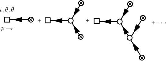
Fig. 1: Treelike graphs of the iterative solution ${\bf\Psi}(t,p,\theta,\bar{\theta})$.

4.3 Iterative solution of the Wess-Zumino flow

The flowed field $\Psi(t,z)$ satisfying the Wess-Zumino flow equation can be expressed as an iterative expansion. To show this, we first introduce a heat kernel in the superspace $z=(x_{\mu},\theta_{\alpha},\bar{\theta}_{\dot{\alpha}})$ as

$${\bf K}_{t}(z)=\left(\begin{array}[]{cc}C_{t}(x)&-\frac{\bar{D}^{2}}{4\sqrt{-\Box}}S_{t}(x)\\ -\frac{D^{2}}{4\sqrt{-\Box}}S_{t}(x)&C_{t}(x)\end{array}\right)\times\delta^{2}(\theta)\delta^{2}(\bar{\theta})$$ (80)

where

$$C_{t}(x) \equiv\int\frac{d^{4}p}{(2\pi)^{4}}e^{ipx-tp^{2}}\cos(tM\sqrt{p^{2}}),$$ (81)

$$S_{t}(x) \equiv\int\frac{d^{4}p}{(2\pi)^{4}}e^{ipx-tp^{2}}\sin(tM\sqrt{p^{2}}).$$ (82)

The heat kernel satisfies

$$\left(\partial_{t}-\Box-M{\bf\Gamma\Delta}\right){\bf K}_{t}(z)=0$$ (83)

and

$${\bf K}_{0}(z)=\delta^{8}(z),$$ (84)

since $C_{0}(x)=\delta^{4}(x)$ and $S_{0}(x)=0$. The flow equation (57) can be solved formally as

$${\bf\Psi}(t,z)=\int d^{8}z^{\prime}{\bf K}_{t}(z-z^{\prime}){\bf\Phi}_{0}(z^{\prime})+\int_{0}^{t}ds\int d^{8}z^{\prime}\bar{\bf\Delta}{\bf K}_{t-s}(z-z^{\prime}){\bf N}(s,z^{\prime}),$$ (85)

where $\bar{\bf\Delta}$ acts on $z$. Inserting the formal solution into ${\bf\Psi}$ of ${\bf N}$ on the rhs repeatedly yields an iterative approximation of the flow equation. The iterative approximation can be expressed as a treelike graph with ${\bf\Phi}_{0}$ at end points.

In Fig. 1, the iterative solution of the Wess-Zumino flow equation (57) is represented graphically. The circle with cross associated with the end points of the flow time zero is a one-point vertex defined by

(86)

The flow vertex shown by an open circle is defined as

(87)

where an operator $\bar{\bf\Delta}_{ii}(p,\theta,\bar{\theta})$ acts upon the outgoing line with the index $i$. For each vertex (one-point and flow vertex), the Grassmann integral $\int d^{2}\theta d^{2}\bar{\theta}$ is performed. In addition, for the flow vertex, the flow time $t$ is integrated out from $0$ to $\infty$.

The flow line connecting the vertices is defined by

(88)

where ${\bf\tilde{K}}_{t}(p,\theta,\bar{\theta})=\int d^{4}xe^{-ipx}{\bf K}_{t}(x,\theta,\bar{\theta})$ and $\Theta(t)$ is the Heaviside step function. The arrow indicates the direction of increasing flow time.

As for the momenta, at each flow vertex, the momentum conservation is assumed, and an undermined momentum of ingoing flow lines is integrated.

In Fig. 1, the treelike graph begins at a single square of flow time $t$ and terminates at the one-point vertices of flow time $0$. The flow time runs from $0$ to $t$ keeping the time order with step functions. The initial condition (73) tells us that this iterative approximation may be understood as the perturbative expansion of one-third power of the coupling constant $g^{\frac{1}{3}}$.

4.4 Super-Feynman rules

We move on to perturbative calculations of correlation functions of ${\bf\Psi}_{i}$ combining the above iterative approximation of the Wess-Zumino flow and the super-Feynman rules in the Wess-Zumino model at $t=0$ discussed in Sec. 3.2.

For example, the leading order contribution to the two-point function is diagrammatically represented as

$$\begin{minipage}[c]{284.52756pt} \centering\includegraphics[width=227.62204pt]{fig01new.pdf} \@add@centering\end{minipage}.$$ (89)

The staple symbol on the lhs denotes the contraction between two boundary fields ${\bf\Phi}_{0}$, which is given at the leading order as

$$\begin{split}&\langle{\bf\Phi}_{0,i}(p,\theta,\bar{\theta}){\bf\Phi}_{0,j}(p^{\prime},\theta^{\prime},\bar{\theta}^{\prime})\rangle\\ &\qquad=g^{\frac{2}{3}}{\bf D}_{ij}(p,\theta,\bar{\theta})\ (2\pi)^{4}\delta^{4}(p+p^{\prime})\delta^{2}(\theta-\theta^{\prime})\delta^{2}(\bar{\theta}-\bar{\theta}^{\prime}),\end{split}$$ (90)

where

$${\bf D}(p,\theta,\bar{\theta})=\frac{1}{\sqrt{p^{2}+m^{2}}}\left(\begin{array}[]{cc}{\rm sin}\left(\beta_{0}(p)\right)\frac{\bar{D}^{2}}{4}&{\rm cos}\left(\beta_{0}(p)\right)\frac{\bar{D}^{2}D^{2}}{16\sqrt{p^{2}}}\\ {\rm cos}\left(\beta_{0}(p)\right)\frac{D^{2}\bar{D}^{2}}{16\sqrt{p^{2}}}&{\rm sin}\left(\beta_{0}(p)\right)\frac{D^{2}}{4}\end{array}\right)$$ (93)

for ${\rm tan}(\beta_{0}(p))=m/\sqrt{p^{2}}$.

As shown in Eq. (89), we obtain the two-point function of $\bf\Psi$ at the leading order taking a contraction between two $\bf\Phi_{0}$ for two tree-level solutions of $\bf\Psi$ as

$$\begin{split}&\langle{\bf\Psi}_{i}(t,p,\theta,\bar{\theta}){\bf\Psi}_{j}(s,q,\theta^{\prime},\bar{\theta}^{\prime})\rangle\\ &\qquad=g^{\frac{2}{3}}{\bf D}_{t+s,ij}(p,\theta,\bar{\theta})\ (2\pi)^{4}\delta^{4}(p+q)\delta^{2}(\theta-\theta^{\prime})\delta^{2}(\bar{\theta}-\bar{\theta}^{\prime}),\end{split}$$ (94)

where

$${\bf D}_{t}(p,\theta,\bar{\theta})=\frac{e^{-tp^{2}}}{\sqrt{p^{2}+m^{2}}}\left(\begin{array}[]{cc}{\rm sin}\left(\beta_{t}(p)\right)\frac{\bar{D}^{2}}{4}&{\rm cos}\left(\beta_{t}(p)\right)\frac{\bar{D}^{2}D^{2}}{16\sqrt{p^{2}}}\\ {\rm cos}\left(\beta_{t}(p)\right)\frac{D^{2}\bar{D}^{2}}{16\sqrt{p^{2}}}&{\rm sin}\left(\beta_{t}(p)\right)\frac{D^{2}}{4}\end{array}\right)$$ (97)

for $\beta_{t}(p)=\beta_{0}(p)+tM\sqrt{p^{2}}$.

Thus, a field propagator associated with Eq.(94) is defined by

(98)

The time dependence appears as a sum of two boundary times, and the diagram of field propagator is shown by a line without an arrow. Since Eq. (97) reproduces Eq. (93) for $t=0$, Eq. (98) contains all of the field propagators such as $\langle{\bf\Phi}_{0}{\bf\Phi}_{0}\rangle$ and the mixed one $\langle{\bf\Phi}_{0}{\bf\Psi}\rangle$, as well as $\langle{\bf\Psi\Psi\rangle}$. Note that each field propagator is counted as $g^{\frac{2}{3}}$ in the perturbation theory.

We reformulate the perturbation theory at $t=0$ in terms of ${\bf\Phi}_{0}$ because the ${\bf\Phi}_{0}$ propagator is treated uniformly with flow propagators. Unlike the perturbation theory given in Sec. 3.2, the GRS propagator $\Delta_{GRS}$ is not used. The super-Feynman rules at $t=0$ should be modified to make fit with the rules for the iterative approximation of the Wess-Zumino flow equation. First, we rewrite the interaction part of the action (20) as

$$S_{int}=-\int d^{8}z\left\{\frac{1}{3!}h_{ijk}\left(\frac{{\bf\Delta}}{\Box}{\bf\Phi}_{0}\right)_{i}{\bf\Phi}_{0,j}{\bf\Phi}_{0,k}\right\}(z),$$ (99)

where $h_{ijk}=2\delta_{ij}\delta_{ik}$. The three-point vertex of the flow time zero may be defined by

$$\begin{minipage}[l]{142.26378pt} \centering\includegraphics[width=71.13188pt]{fig4new3.pdf} \@add@centering\end{minipage}=\hskip 22.76219pt-h_{ijk}\frac{{\bf\Delta}_{ii}(p,\theta,\bar{\theta})}{p^{2}},$$ (100)

where ${\bf\Delta}_{ii}(p,\theta,\bar{\theta})$ acts on an internal line $p,i$. This is because ${\bf\Delta}_{ii}(p,\theta,\bar{\theta})/p^{2}$ can be changed to ${\bf\Delta}_{jj}(q,\theta,\bar{\theta})/q^{2}$ or ${\bf\Delta}_{kk}(r,\theta,\bar{\theta})/r^{2}$ by using the identity $\frac{\bar{\bf\Delta}{\bf\Delta}}{\Box}{\bf\Phi}_{0}={\bf\Phi}_{0}$ for Eq.(99). For each boundary vertex, the Grassmann integral $\int d^{2}\theta d^{2}\bar{\theta}$ is performed.

Now, we consider the following one-loop correction to the two-point function, including one flow vertex (open circle) and one ordinary vertex (filled circle):

$$\begin{minipage}[c]{284.52756pt} \centering\includegraphics[width=341.43306pt]{fig02new.pdf} \@add@centering\end{minipage}\hskip 56.9055pt.$$ (101)

As in the tree-level case, performing the contraction between two ${\bf\Phi}_{0}$ yields a field propagator. In this case, the three lines without arrows on the rhs indicate the mixed propagators associated with $\langle{\bf\Phi}_{0}{\bf\Psi}\rangle$.

Here, we mention that the coupling expansion does not naively correspond to the loop expansion. This is because the $g$ dependence arises only from the field propagators of the order $g^{2/3}$, and the vertices and flow propagator do not depend on $g$. Each one-loop diagram in Fig. 2 has different orders $g^{2n/3}$ where $n$ is the number of field propagators.

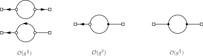
Fig. 2: One-loop diagrams

The super-Feynman rules for the correlation functions of ${\bf\Psi}$ in the momentum space are summarized as follows:

• Use Eq.(88) for a flow line that is an outgoing line emanated from each flow vertex.

• Use Eq.(98) for a field propagator by which two points (flow vertices, boundary vertices, and starting points denoted by $\square$) are connected.

• Use Eq.(87) for each flow vertex, and use Eq.(100) for each boundary vertex. For each flow vertex at $t$, perform the flow time integral $\int_{0}^{\infty}dt$. For all the flow and boundary vertices at $(\theta,\bar{\theta})$, perform the Grassmann integral $\int d^{2}\theta d^{2}\bar{\theta}$.

• Impose the momentum conservation at each vertex and integrate over undetermined loop momenta.

• Compute the usual combinatoric factors.

These rules are given in Euclidean space. In addition, we mention rules and properties that are common with the Yang-Mills flow[2]. Diagrams with closed flow line loops are absent because any loop has at least a field propagator. The flow lines depend on the difference between two flow times of end points. The flow time dependence of propagators are determined by the sum of flow times at the end points.

4.5 The massive free flow

We consider the massive free flow, dropping the interaction terms from the flow equations (but the boundary Wess-Zumino model has the interactions). The exact solution is

$${\bf\Psi}(t,z)=\int d^{8}z^{\prime}{\bf K}_{t}(z-z^{\prime}){\bf\Phi}_{0}(z^{\prime}).$$ (102)

Then, recalling the definition of ${\bf\Phi}_{0}$ (73), a correlation function of the flowed fields $\langle{\bf\Psi}(t_{1},z_{1}){\bf\Psi}(t_{2},z_{2})\ldots{\bf\Psi}(t_{n},z_{n})\rangle$ can be given by a linear combination of correlation functions of the renormalized fields $\Phi_{R}(z_{i})$ and $\bar{\Phi}_{R}(z_{i})$ with $(g_{R})^{\frac{n}{3}}$. In the renormalized perturbation theory, when evaluating the correlators of $\Phi_{R}(z_{i})$ and $\bar{\Phi}_{R}(z_{i})$, UV divergences are renormalized by the normal counterterms. So, in the case of the massive free flow, any correlation function of the flowed fields is UV finite for any nonzero flow time if the Wess-Zumino model is properly renormalized.

4.6 Power counting theorem

We can calculate the superficial degrees of divergence in the perturbation theory of the Wess-Zumino flow using the super-Feynman rule given in Sec. 4.4.

Since the field propagators given in Eq. (98) have $t$-dependent functions, we need to evaluate the following integrals for each flow vertex:

$$I(p^{2})\equiv\int_{0}^{\infty}dte^{-tp^{2}}f(t,p^{2}),$$ (103)

where $p$ is a loop momentum and external momenta are set to zero for simplicity. After a short calculation, we find that, for large $p^{2}$,

$$I(p^{2})=p^{-2}f(0,p^{2})+\left(p^{-2}\right)^{2}f^{(1)}(0,p^{2})+\cdots,$$ (104)

where $f^{(n)}(t,p^{2})=d^{n}f(t,p^{2})/dt^{n}$. Since flow propagators with the same chirality and field propagators have $f(t,p^{2})\sim{\rm cos}(tM\sqrt{p^{2}})$, ${\rm cos}(\beta_{t}(p^{2}))$, ${\rm sin}(\beta_{t}(p^{2}))$, the extra suppression factor appears as $p^{-2}$ from the first term of (104). Whereas, for massive flow propagators with the opposite chirality, $f(t,p^{2})\sim{\rm sin}(tM\sqrt{p^{2}})$ leads to $f(0,p^{2})=0$ and the extra factor becomes $p^{-3}$ from the second term of (104).

At each flow vertex with an external flow line, we can apply the identity $\frac{\bar{\bf\Delta}{\bf\Delta}}{\Box}{\bf\Psi}={\bf\Psi}$ to an internal line and move a factor of $\bar{\bf\Delta}$ to the external line by integrals of parts. This transformation leads to an extra suppression factor $p^{-1}$ because a factor $\frac{{\bf\Delta}}{\Box}$ remains at the internal line. This type of transformation cannot be applied to the boundary vertex because, since it is made of fields with the same chirality, the partial integration of $\bar{\bf\Delta}$ does not work.

Consider a 1PI supergraph with $L$ loops, $V$ boundary vertices, $V_{f}$ flow vertices, $E$ external field lines, $E_{f}$ external flow lines, and $P$ field propagators, of which $C$ are massive field propagators with the same chirality, $\Psi\Psi$ and $\bar{\Psi}\bar{\Psi}$, and $P_{f}$ flow propagators, of which $C_{f}$ are massive flow propagators with the opposite chirality. Each loop has a $d^{4}p$ integral, and the identity $\delta_{12}D^{2}\bar{D}^{2}\delta_{12}=16\delta_{12}$ still applies in this case to remove a $D^{2}\bar{D}^{2}\sim p^{2}$ at each loop. At $t=0$, $\Psi\bar{\Psi}$ propagators behave as $p^{0}$, while massive chiral propagators behave as $p^{-1}$ for large $p^{2}$. We have extra suppression factors $p^{-2}$ from the boundary of $t$ integrations at each flow vertex discussed above. For massive flow propagators with the opposite chirality, we have $p^{-3}$ instead of $p^{-2}$. Each boundary vertex has a factor of ${\bf\Delta}_{ii}/p^{2}\sim p^{-1}$ on one of the internal lines. Each internal outgoing flow line emanated from the flow vertex has a factor of $\bar{\bf\Delta}_{ii}\sim p$. Each external flow line has a suppression factor $p^{-1}$ from the discussion using the identity $\frac{\bar{\bf\Delta}{\bf\Delta}}{\Box}{\bf\Psi}={\bf\Psi}$.

Thus, we find that the superficial degrees of divergence $d$ is given by

$$d=2L-C-2V_{f}-C_{f}-V+V_{f}-E_{f}-E_{f}.$$ (105)

Using a topology relation $L-P-P_{f}+V+V_{f}=1$ and a few relations such as $3V+3V_{f}=E+E_{f}+2P+2P_{f}$ (each vertex has three lines) and $V_{f}=E_{f}+P_{f}$ (the flow vertex has an outgoing flow line), where $E_{f}\geq 1$ for nonzero $V_{f}$, we finally obtain

$$d=2-C-C_{f}-E-3E_{f}.$$ (106)

This shows that any super-Feynman graph with flow vertices is UV finite at all orders of perturbation theory. The remaining divergences for $V_{f}=E_{f}=0$ arise from boundary vertices and cancel as in the massive free flow case because $n$-point functions of ${\bf\Psi}(t,z)$ are those of ${\bf K}_{t}{\bf\Phi}_{0}(z)$ for $V_{f}=0$ and ${\bf\Phi}_{0}$ is given by $g_{R}$ and renormalized fields $\Phi_{R}$ from (73). We can conclude that any correlation function of flowed fields is UV finite in the Wess-Zumino flow at all orders of perturbation theory.

5 Summary

We introduced a supersymmetric gradient flow with renormalization-invariant couplings in the Wess-Zumino model and showed that correlation functions of the flowed superfield are UV finite using a power counting theorem for 1PI supergraphs based on super-Feynman rules. In particular, we found that the interaction terms of the flow equation do not contribute to divergent graphs, only terms of the boundary theory do. After the parameter renormalization in the boundary theory, the remaining divergence of the wave function can be removed by taking initial conditions to be renormalization invariant. Thus, we found that any correlation function of the flowed superfield is UV finite at all orders of the perturbation theory.

In nonsupersymmetric scalar field theory, including the mass term and a term like $\phi^{4}$ interaction yields nonremovable divergences. Even in the massless free flow, a wave function renormalization remains. Some kind of symmetry could be necessary for the UV finiteness property. In the Yang-Mills flow, the BRS symmetry guarantees the UV finiteness, whereas in the Wess-Zumino flow the supersymmetry plays a crucial role to hold the property in a mechanism that is quite different from the Yang-Mills flow.

The existence of the nonrenormalization theorem is significant in our proof because it leads to the renormalization-invariant initial condition [Eqs. (68) and (73)] and the invariant mass [Eq. (13)] in the Wess-Zumino flow [Eq. (57)]. The UV finiteness is a direct consequence of these invariances. Therefore, it is unclear whether our results can be extended to other theories that do not have a nonrenormalization theorem.

Without the renormalization-invariant initial conditions (68) and (73), the wave function renormalization remains, and the extra wave function renormalization of the flowed superfield, as in gradient flow of quark fields, makes the correlation function finite. On the other hand, if the flow equations are not given by renormalization-invariant coupling constants, the perturbative renormalizability breaks down completely.

Gradient flows have been successfully applied to various research such as nonperturbative renormalization group, holographic descriptions of field theory, and lattice simulations. In addition, supersymmetry has been actively studied in particle physics in a variety of ways. Therefore, supersymmetric gradient flows can be expected to have various applications. The techniques developed in this article will be very useful for subsequent studies using supersymmetric gradient flows.

Appendix A Convention in Euclidean space

In order to obtain the Euclidean theory from the Minkowski one with metric $\eta_{\mu\nu}={\rm diag}\{-1,1,1,1\}$ in Ref. [52], we use the Wick rotation $x_{0}\rightarrow-ix_{0}$ to move on to the Euclidean signature. The Euclidean four-dimensional $\sigma$ matrices are defined as $\sigma_{0}=\bar{\sigma}_{0}\equiv-i\mathbf{1}$; the others are the same. The auxiliary fields in the chiral superfields are replaced as $F,F^{*}\rightarrow iF,iF^{*}$. The Euclidean action is defined as $S_{E}=-iS$ after the Wick rotation.

The Fourier transformation is defined by

$$\Phi(x,\theta,\bar{\theta})=\int\frac{d^{4}p}{(2\pi)^{4}}e^{ipx}\tilde{\Phi}(p,\theta,\bar{\theta}).$$ (107)

A.1 Spinors and $\sigma$ matrices

Let $\psi_{\alpha}$ ($\alpha=1,2$) be a $SU(2)_{R}$ spinor and $\bar{\psi}_{\dot{\alpha}}$ ($\dot{\alpha}=1,2$) be a $SU(2)_{L}$ spinor, then they are not related to each other under the complex conjugate in the four-dimensional Euclidian space. We define the invariant tensors of $SU(2)_{R}$ and $SU(2)_{L}$ as

$$\epsilon_{21}=\epsilon^{12}=\epsilon_{\dot{2}\dot{1}}=\epsilon^{\dot{1}\dot{2}}=1,\quad\epsilon_{12}=\epsilon^{21}=\epsilon_{\dot{1}\dot{2}}=\epsilon^{\dot{2}\dot{1}}=-1$$ (108)

with the others being zero, so that $\epsilon_{\alpha\beta}\epsilon^{\beta\gamma}=\delta_{\alpha}{}^{\gamma}$ and $\epsilon_{\dot{\alpha}\dot{\beta}}\epsilon^{\dot{\beta}\dot{\gamma}}=\delta_{\dot{\alpha}}{}^{\dot{\gamma}}$. Then spinors with upper and lower indices are related through the invariant tensors,

$$\psi^{\alpha}=\epsilon^{\alpha\beta}\psi_{\beta},\quad\psi_{\alpha}=\epsilon_{\alpha\beta}\psi^{\beta}.$$ (109)

We use the following spinor summation convention:

$$\psi\chi=\psi^{\alpha}\chi_{\alpha},\qquad\bar{\psi}\bar{\chi}=\bar{\psi}_{\dot{\alpha}}\bar{\chi}^{\dot{\alpha}}.$$ (110)

The $\sigma$ matrices in the Euclidean space $(\sigma_{\mu})_{\alpha\dot{\beta}}$ and $(\bar{\sigma}_{\mu})^{\dot{\alpha}\beta}$ are defined as

$$\sigma_{0}=\left(\begin{array}[]{cc}-i&0\\ 0&-i\end{array}\right),\qquad\sigma_{1}=\left(\begin{array}[]{cc}0&1\\ 1&0\end{array}\right),$$ (115)

$$\sigma_{2}=\left(\begin{array}[]{cc}0&-i\\ i&0\end{array}\right),\qquad\sigma_{3}=\left(\begin{array}[]{cc}1&0\\ 0&-1\end{array}\right),$$ (120)

$$(\bar{\sigma}_{\mu})^{\dot{\alpha}\alpha}=\epsilon^{\dot{\alpha}\dot{\beta}}\epsilon^{\alpha\beta}(\sigma_{\mu})_{\beta\dot{\beta}},$$

$$\bar{\sigma}_{0}=\sigma_{0},\qquad\bar{\sigma}_{i}=-\sigma_{i}\ \ (i=1,2,3).$$

For more detail on the spinor algebra, see Ref. [30].

A.2 Chiral superfield

The supercharges $Q_{\alpha}$ and $\bar{Q}_{\dot{\alpha}}$ are defined as difference operators on the superspace labeled by $z=(x_{\mu},\theta_{\alpha},\bar{\theta}_{\dot{\alpha}})$,

$$\begin{split}&Q_{\alpha}={\partial_{\alpha}}-i(\sigma_{\mu})_{\alpha\dot{\alpha}}\bar{\theta}^{\dot{\alpha}}\partial_{\mu}\\ &\bar{Q}_{\dot{\alpha}}=-{\partial_{\dot{\alpha}}}+i\theta^{\alpha}(\sigma_{\mu})_{\alpha\dot{\alpha}}\partial_{\mu},\end{split}$$ (121)

where $\partial_{\alpha}=\frac{\partial}{\partial\theta^{\alpha}},\ \partial_{\dot{\alpha}}=\frac{\partial}{\partial\bar{\theta}^{\dot{\alpha}}}$, and $\partial_{\mu}=\frac{\partial}{\partial x_{\mu}}$. The associated supercovariant derivatives that commute with the supercharges are defined as

$$\begin{split}&D_{\alpha}={\partial_{\alpha}}+i(\sigma_{\mu})_{\alpha\dot{\alpha}}\bar{\theta}^{\dot{\alpha}}\partial_{\mu}\\ &\bar{D}_{\dot{\alpha}}=-{\partial_{\dot{\alpha}}}-i\theta^{\alpha}(\sigma_{\mu})_{\alpha\dot{\alpha}}\partial_{\mu}.\end{split}$$ (122)

These difference operators obey

$$\begin{split}&\{Q_{\alpha},\bar{Q}_{\dot{\alpha}}\}=2i(\sigma_{\mu})_{\alpha\dot{\alpha}}\partial_{\mu}\\ &\{D_{\alpha},\bar{D}_{\dot{\alpha}}\}=-2i(\sigma_{\mu})_{\alpha\dot{\alpha}}\partial_{\mu}\end{split}$$ (123)

and the other anticommutation relations vanish. After a short calculation, one can show the useful identities

$$\begin{split}D^{2}\bar{D}^{2}D^{2}=&16\Box D^{2},\\ \bar{D}^{2}D^{2}\bar{D}^{2}=&16\Box\bar{D}^{2},\end{split}$$ (124)

where $\Box=\partial_{\mu}\partial_{\mu}$.

The chiral and antichiral superfields $\Phi(x,\theta,\bar{\theta})$ and $\bar{\Phi}(x,\theta,\bar{\theta})$ are characterized by the constraints $\bar{D}_{\dot{\alpha}}\Phi=0$ and $D_{\alpha}\bar{\Phi}=0$, respectively. They are expanded in $\theta$ and $\bar{\theta}$ as

$$\Phi(x,\theta,\bar{\theta})= A(x)+i\theta\sigma_{\mu}\bar{\theta}\partial_{\mu}A(x)+\frac{1}{4}\theta\theta\bar{\theta}\bar{\theta}\Box A(x)$$

$$+\sqrt{2}\theta\psi(x)-\frac{i}{\sqrt{2}}\theta\theta\partial_{\mu}\psi(x)\sigma_{\mu}\bar{\theta}+i\theta\theta F(x),$$ (125)

$$\bar{\Phi}(x,\theta,\bar{\theta})= A^{*}(x)-i\theta\sigma_{\mu}\bar{\theta}\partial_{\mu}A^{*}(x)+\frac{1}{4}\theta\theta\bar{\theta}\bar{\theta}\Box A^{*}(x)$$

$$+\sqrt{2}\bar{\theta}\bar{\psi}(x)+\frac{i}{\sqrt{2}}\bar{\theta}\bar{\theta}\theta\sigma_{\mu}\partial_{\mu}\bar{\psi}(x)+i\bar{\theta}\bar{\theta}F^{*}(x),$$ (126)

where $A$ and $F$ are complex bosonic fields, and $\psi,\bar{\psi}$ are two component spinors. Note that $\bar{\Phi}$ is not a complex conjugate of $\Phi$ in this Euclidean theory. One can easily find the following projection operators for the chiral superfields:

$$\frac{\bar{D}^{2}D^{2}}{16\Box}\Phi=\Phi,$$ (127)

$$\frac{D^{2}\bar{D}^{2}}{16\Box}\bar{\Phi}=\bar{\Phi}.$$ (128)

Introducing new coordinate $(y,\theta,\bar{\theta})$ with $y_{\mu}=x_{\mu}+i\theta\sigma_{\mu}\bar{\theta}$, the derivative operators and $\Phi$ are expressed as

$$\begin{split}&Q_{\alpha}={\partial_{\alpha}},\\ &\bar{Q}_{\dot{\alpha}}=-{\partial_{\dot{\alpha}}}+2i\theta^{\alpha}(\sigma_{\mu})_{\alpha\dot{\alpha}}\partial_{\mu},\\ &D_{\alpha}={\partial_{\alpha}}+2i(\sigma_{\mu})_{\alpha\dot{\alpha}}\bar{\theta}^{\dot{\alpha}}\partial_{\mu},\\ &\bar{D}_{\dot{\alpha}}=-{\partial_{\dot{\alpha}}},\\ &\Phi(y,\theta)=A(y)+\sqrt{2}\theta\psi(y)+i\theta\theta F(y),\end{split}$$ (129)

while in $(\bar{y},\theta,\bar{\theta})$ with $\bar{y}_{\mu}=x_{\mu}-i\theta\sigma_{\mu}\bar{\theta}$,

$$\begin{split}&Q_{\alpha}={\partial_{\alpha}}-2i(\sigma_{\mu})_{\alpha\dot{\alpha}}\bar{\theta}^{\dot{\alpha}}\partial_{\mu},\\ &\bar{Q}_{\dot{\alpha}}=-{\partial_{\dot{\alpha}}},\\ &D_{\alpha}={\partial_{\alpha}},\\ &\bar{D}_{\dot{\alpha}}=-{\partial_{\dot{\alpha}}}-2i\theta^{\alpha}(\sigma_{\mu})_{\alpha\dot{\alpha}}\partial_{\mu},\\ &\bar{\Phi}(\bar{y},\bar{\theta})=A^{*}(\bar{y})+\sqrt{2}\bar{\theta}\bar{\psi}(\bar{y})+i\bar{\theta}\bar{\theta}F^{*}(\bar{y}).\end{split}$$ (130)

Note that $\bar{y}$ is not a complex conjugate of $y$ in the Euclidean space.

A.3 Integral and delta function over Grassmann coordinates

The volume element of the superspace $z=(x_{\mu},\theta_{\alpha},\bar{\theta}_{\dot{\alpha}})$ is

$$d^{8}z=d^{4}x\,d^{2}\theta\,d^{2}\bar{\theta},$$ (131)

where

$$\int d^{2}\theta\,\theta^{2}=1,\quad\int d^{2}\bar{\theta}\,\bar{\theta}^{2}=1.$$ (132)

Under the Euclidean space integral, the Grassmann integrals can be interpreted as

$$\int d^{4}x\,d^{2}\theta=\int d^{4}x\,\left(-\frac{D^{2}}{4}\right),\quad\int d^{4}x\,d^{2}\bar{\theta}=\int d^{4}x\,\left(-\frac{\bar{D}^{2}}{4}\right)$$ (133)

and

$$\int d^{4}x\,d^{2}\theta\,d^{2}\bar{\theta}=\int d^{4}x\,\left(\frac{D^{2}\bar{D}^{2}}{16}\right).$$ (134)

The delta functions are defined as

$$\delta^{2}(\theta)=\theta^{2},\quad\delta^{2}(\bar{\theta})=\bar{\theta}^{2},$$ (135)

such that

$$\int d^{2}\theta\,\delta^{2}(\theta)=1,\quad\int d^{2}\bar{\theta}\,\delta^{2}(\bar{\theta})=1.$$ (136)

The functional derivatives of chiral superfields $\Phi(z)$ and $\bar{\Phi}(z)$ are

$$\frac{\delta\Phi(z_{1})}{\delta\Phi(z_{2})}=-\frac{\bar{D}_{1}^{2}}{4}\delta^{8}(z_{1}-z_{2}),$$ (137)

$$\frac{\delta\bar{\Phi}(z_{1})}{\delta\bar{\Phi}(z_{2})}=-\frac{D_{1}^{2}}{4}\delta^{8}(z_{1}-z_{2}),$$ (138)

where

$$\delta^{8}(z_{1}-z_{2})=\delta^{4}(x_{1}-x_{2})\delta^{2}(\theta_{1}-\theta_{2})\delta^{2}(\bar{\theta}_{1}-\bar{\theta}_{2}).$$ (139)

We use the abbreviation $\delta_{12}=\delta^{2}(\theta_{1}-\theta_{2})\delta^{2}(\bar{\theta}_{1}-\bar{\theta}_{2})$ for simplicity. The following relation

$$\delta_{12}D^{2}\bar{D}^{2}\delta_{21}=\delta_{12}\bar{D}^{2}D^{2}\delta_{21}=16\delta_{12}$$ (140)

is useful in perturbative calculations.

References

- [1] M. Lüscher, “Properties and uses of the Wilson flow in lattice QCD,” JHEP 08 (2010) 071, arXiv:1006.4518 [hep-lat]. [Erratum: JHEP03,092(2014)].
- [2] M. Luscher and P. Weisz, “Perturbative analysis of the gradient flow in non-abelian gauge theories,” JHEP 02 (2011) 051, arXiv:1101.0963 [hep-th].
- [3] R. Yamamura, “The Yang-Mills gradient flow and lattice effective action,” PTEP 2016 no. 7, (2016) 073B10, arXiv:1510.08208 [hep-lat].
- [4] H. Makino, O. Morikawa, and H. Suzuki, “Gradient flow and the Wilsonian renormalization group flow,” PTEP 2018 no. 5, (2018) 053B02, arXiv:1802.07897 [hep-th].
- [5] Y. Abe and M. Fukuma, “Gradient flow and the renormalization group,” PTEP 2018 no. 8, (2018) 083B02, arXiv:1805.12094 [hep-th].
- [6] A. Carosso, A. Hasenfratz, and E. T. Neil, “Nonperturbative Renormalization of Operators in Near-Conformal Systems Using Gradient Flows,” Phys. Rev. Lett. 121 no. 20, (2018) 201601, arXiv:1806.01385 [hep-lat].
- [7] H. Sonoda and H. Suzuki, “Derivation of a gradient flow from the exact renormalization group,” PTEP 2019 no. 3, (2019) 033B05, arXiv:1901.05169 [hep-th].
- [8] H. Sonoda and H. Suzuki, “Gradient flow exact renormalization group,” PTEP 2021 no. 2, (2021) 023B05, arXiv:2012.03568 [hep-th].
- [9] Y. Miyakawa and H. Suzuki, “Gradient flow exact renormalization group: Inclusion of fermion fields,” PTEP 2021 no. 8, (2021) 083B04, arXiv:2106.11142 [hep-th].
- [10] Y. Miyakawa, H. Sonoda, and H. Suzuki, “Manifestly gauge invariant exact renormalization group for quantum electrodynamics,” PTEP 2022 no. 2, (2022) 023B02, arXiv:2111.15529 [hep-th].
- [11] Y. Miyakawa, “Axial anomaly in the gradient flow exact renormalization group,” arXiv:2201.08181 [hep-th].
- [12] H. Sonoda and H. Suzuki, “One-particle irreducible Wilson action in the gradient flow exact renormalization group formalism,” PTEP 2022 no. 5, (2022) 053B01, arXiv:2201.04448 [hep-th].
- [13] A. Hasenfratz, C. J. Monahan, M. D. Rizik, A. Shindler, and O. Witzel, “A novel nonperturbative renormalization scheme for local operators,” PoS LATTICE2021 (2022) 155, arXiv:2201.09740 [hep-lat].
- [14] Y. Abe, Y. Hamada, and J. Haruna, “Fixed point structure of the gradient flow exact renormalization group for scalar field theories,” PTEP 2022 no. 3, (2022) 033B03, arXiv:2201.04111 [hep-th].
- [15] S. Aoki, K. Kikuchi, and T. Onogi, “Geometries from field theories,” PTEP 2015 no. 10, (2015) 101B01, arXiv:1505.00131 [hep-th].
- [16] S. Aoki, J. Balog, T. Onogi, and P. Weisz, “Flow equation for the large scalar model and induced geometries,” PTEP 2016 no. 8, (2016) 083B04, arXiv:1605.02413 [hep-th].
- [17] S. Aoki and S. Yokoyama, “AdS geometry from CFT on a general conformally flat manifold,” Nucl. Phys. B933 (2018) 262–274, arXiv:1709.07281 [hep-th].
- [18] S. Aoki and S. Yokoyama, “Flow equation, conformal symmetry, and anti-de Sitter geometry,” PTEP 2018 no. 3, (2018) 031B01, arXiv:1707.03982 [hep-th].
- [19] S. Aoki, J. Balog, and S. Yokoyama, “Holographic computation of quantum corrections to the bulk cosmological constant,” PTEP 2019 no. 4, (2019) 043B06, arXiv:1804.04636 [hep-th].
- [20] S. Aoki, S. Yokoyama, and K. Yoshida, “Holographic geometry for nonrelativistic systems emerging from generalized flow equations,” Phys. Rev. D 99 no. 12, (2019) 126002, arXiv:1902.02578 [hep-th].
- [21] S. Aoki, J. Balog, T. Onogi, and S. Yokoyama, “Special flow equation and the GKP–Witten relation,” PTEP 2023 no. 1, (2023) 013B03, arXiv:2204.06855 [hep-th].
- [22] H. Makino, F. Sugino, and H. Suzuki, “Large- limit of the gradient flow in the 2D nonlinear sigma model,” PTEP 2015 no. 4, (2015) 043B07, arXiv:1412.8218 [hep-lat].
- [23] S. Aoki, K. Kikuchi, and T. Onogi, “Gradient Flow of O(N) nonlinear sigma model at large N,” JHEP 04 (2015) 156, arXiv:1412.8249 [hep-th].
- [24] H. Makino and H. Suzuki, “Renormalizability of the gradient flow in the 2D non-linear sigma model,” PTEP 2015 no. 3, (2015) 033B08, arXiv:1410.7538 [hep-lat].
- [25] S. Aoki, J. Balog, T. Onogi, and P. Weisz, “Flow equation for the scalar model in the large expansion and its applications,” PTEP 2017 no. 4, (2017) 043B01, arXiv:1701.00046 [hep-th].
- [26] N. Nakazawa, “N=1 superYang-Mills theory in Ito calculus,” Prog. Theor. Phys. 110 (2004) 1117–1150, arXiv:hep-th/0302138 [hep-th].
- [27] N. Nakazawa, “Stochastic gauge fixing in N=1 supersymmetric Yang-Mills theory,” Prog. Theor. Phys. 116 (2007) 883–917, arXiv:hep-th/0308081 [hep-th].
- [28] K. Kikuchi and T. Onogi, “Generalized Gradient Flow Equation and Its Application to Super Yang-Mills Theory,” JHEP 11 (2014) 094, arXiv:1408.2185 [hep-th].
- [29] S. Aoki, K. Kikuchi, and T. Onogi, “Flow equation of = 1 supersymmetric O(N) nonlinear sigma model in two dimensions,” JHEP 02 (2018) 128, arXiv:1704.03717 [hep-th].
- [30] D. Kadoh and N. Ukita, “Supersymmetric gradient flow in SYM,” Eur. Phys. J. C 82 no. 5, (2022) 435, arXiv:1812.02351 [hep-th].
- [31] D. Kadoh, K. Kikuchi, and N. Ukita, “Supersymmetric gradient flow in the Wess-Zumino model,” Phys. Rev. D100 no. 1, (2019) 014501, arXiv:1904.06582 [hep-th].
- [32] D. Kadoh and N. Ukita, “Gradient flow equation in SQCD,” PoS LATTICE2019 (2020) 199, arXiv:1912.13247 [hep-lat].
- [33] G. Bergner, C. López, and S. Piemonte, “Study of center and chiral symmetry realization in thermal super Yang-Mills theory using the gradient flow,” Phys. Rev. D 100 no. 7, (2019) 074501, arXiv:1902.08469 [hep-lat].
- [34] K. Hieda, A. Kasai, H. Makino, and H. Suzuki, “4D SYM supercurrent in terms of the gradient flow,” PTEP 2017 no. 6, (2017) 063B03, arXiv:1703.04802 [hep-lat].
- [35] A. Kasai, O. Morikawa, and H. Suzuki, “Gradient flow representation of the four-dimensional super Yang–Mills supercurrent,” PTEP 2018 no. 11, (2018) 113B02, arXiv:1808.07300 [hep-lat].
- [36] S. Chigusa, T. Moroi, and Y. Shoji, “Bounce Configuration from Gradient Flow,” Phys. Lett. B 800 (2020) 135115, arXiv:1906.10829 [hep-ph].
- [37] R. Sato, “Simple Gradient Flow Equation for the Bounce Solution,” Phys. Rev. D 101 no. 1, (2020) 016012, arXiv:1907.02417 [hep-ph].
- [38] Y. Hamada and K. Kikuchi, “Obtaining the sphaleron field configurations with gradient flow,” Phys. Rev. D 101 no. 9, (2020) 096014, arXiv:2003.02070 [hep-th].
- [39] D. L. J. Ho and A. Rajantie, “Classical production of ’t Hooft–Polyakov monopoles from magnetic fields,” Phys. Rev. D 101 no. 5, (2020) 055003, arXiv:1911.06088 [hep-th].
- [40] K. Fujikawa, “The gradient flow in theory,” JHEP 03 (2016) 021, arXiv:1601.01578 [hep-lat].
- [41] O. Morikawa and H. Suzuki, “Axial anomaly in a gravitational field via the gradient flow,” PTEP 2018 no. 7, (2018) 073B02, arXiv:1803.04132 [hep-th].
- [42] M. Luscher, “Chiral symmetry and the Yang–Mills gradient flow,” JHEP 04 (2013) 123, arXiv:1302.5246 [hep-lat].
- [43] H. Suzuki, “Energy–momentum tensor from the Yang–Mills gradient flow,” PTEP 2013 (2013) 083B03, arXiv:1304.0533 [hep-lat]. [Erratum: PTEP2015,079201(2015)].
- [44] H. Makino and H. Suzuki, “Lattice energy–momentum tensor from the Yang–Mills gradient flow—inclusion of fermion fields,” PTEP 2014 (2014) 063B02, arXiv:1403.4772 [hep-lat]. [Erratum: PTEP2015,079202(2015)].
- [45] FlowQCD Collaboration, M. Asakawa, T. Hatsuda, E. Itou, M. Kitazawa, and H. Suzuki, “Thermodynamics of SU(3) gauge theory from gradient flow on the lattice,” Phys. Rev. D90 no. 1, (2014) 011501, arXiv:1312.7492 [hep-lat]. [Erratum: Phys. Rev.D92,no.5,059902(2015)].
- [46] Y. Taniguchi, S. Ejiri, R. Iwami, K. Kanaya, M. Kitazawa, H. Suzuki, T. Umeda, and N. Wakabayashi, “Exploring = 2+1 QCD thermodynamics from the gradient flow,” Phys. Rev. D96 no. 1, (2017) 014509, arXiv:1609.01417 [hep-lat]. [Erratum: Phys. Rev.D99,no.5,059904(2019)].
- [47] M. Kitazawa, T. Iritani, M. Asakawa, and T. Hatsuda, “Correlations of the energy-momentum tensor via gradient flow in SU(3) Yang-Mills theory at finite temperature,” Phys. Rev. D96 no. 11, (2017) 111502, arXiv:1708.01415 [hep-lat].
- [48] R. Yanagihara, T. Iritani, M. Kitazawa, M. Asakawa, and T. Hatsuda, “Distribution of Stress Tensor around Static Quark–Anti-Quark from Yang-Mills Gradient Flow,” Phys. Lett. B789 (2019) 210–214, arXiv:1803.05656 [hep-lat].
- [49] R. V. Harlander, Y. Kluth, and F. Lange, “The two-loop energy–momentum tensor within the gradient-flow formalism,” Eur. Phys. J. C78 no. 11, (2018) 944, arXiv:1808.09837 [hep-lat].
- [50] T. Iritani, M. Kitazawa, H. Suzuki, and H. Takaura, “Thermodynamics in quenched QCD: energy–momentum tensor with two-loop order coefficients in the gradient-flow formalism,” PTEP 2019 no. 2, (2019) 023B02, arXiv:1812.06444 [hep-lat].
- [51] F. Capponi, A. Rago, L. Del Debbio, S. Ehret, and R. Pellegrini, “Renormalisation of the energy-momentum tensor in scalar field theory using the Wilson flow,” PoS LATTICE2015 (2016) 306, arXiv:1512.02851 [hep-lat].
- [52] J. Wess and J. Bagger, “Supersymmetry and Supergravity SECOND EDITION, REVISED AND EXPANDED,” Princeton Serieis in Physics Princeton University Press, Princeton, New Jersey (1992).
- [53] J. Wess and B. Zumino, “A Lagrangian Model Invariant Under Supergauge Transformations,” Phys. Lett. B 49 (1974) 52.
- [54] J. Iliopoulos and B. Zumino, “Broken Supergauge Symmetry and Renormalization,” Nucl. Phys. B 76 (1974) 310.
- [55] M. T. Grisaru, W. Siegel, and M. Rocek, “Improved Methods for Supergraphs,” Nucl. Phys. B 159 (1979) 429.
- [56] N. Seiberg, “Naturalness versus supersymmetric nonrenormalization theorems,” Phys. Lett. B 318 (1993) 469–475, arXiv:hep-ph/9309335.