A general basis set algorithm for galactic haloes and discs

We present a unified approach to (bi-)orthogonal basis sets for gravitating systems. Central to our discussion is the notion of mutual gravitational energy, which gives rise to the self-energy inner product on mass densities. We consider a first-order differential operator that is self-adjoint with respect to this inner product, and prove a general theorem that gives the conditions under which a (bi-)orthogonal basis set arises by repeated application of this differential operator. We then show that these conditions are fulfilled by all the families of analytical basis sets with infinite extent that have been discovered to date. The new theoretical framework turns out to be closely connected to Fourier-Mellin transforms, and it is a powerful tool for constructing general basis sets. We demonstrate this by deriving a basis set for the isochrone model and demonstrating its numerical reliability by reproducing a known result concerning unstable radial modes.

1 Introduction

Orthogonal basis sets play a key role in the efficient calculation of the gravitational potential of perturbed, isolated mass distributions. They also have great value for investigating the stability of dynamical models for galaxies. Both these topics have attracted renewed interest recently in light of the mounting observational evidence that the Milky Way and other galaxies are not as symmetric in shape as assumed previously (Vera-Ciro & Helmi, 2013; Law & Majewski, 2010), and moreover may not be in exact dynamical equilibrium (Erkal et al., 2021; Petersen & Peñarrubia, 2021).

A small sample of recent applications of basis sets includes: efficiently reconstructing individual trajectories in time-varying snapshots of $N$-body simulations of dark matter haloes (Lowing et al., 2011; Sanders et al., 2020; Petersen et al., 2022); flexible non-parametric models for the Milky Way (Garavito-Camargo et al., 2021); and a wide variety of perturbation calculations (Hamilton et al., 2018; Fouvry & Prunet, 2022).

The development of these so-called ‘biorthogonal’ basis sets begins with Clutton-Brock (1972, 1973), who introduced two remarkable analytical sets of potential-density pairs based on the Kuzmin (1956) disc and Plummer (1911) sphere respectively. These mathemtical discoveries (along with some later results discussed below), while fortunate, are limited. It has long been recognised that to make best use of the basis set technique, one would prefer a complete freedom in choice of zeroth-order (as well as underlying coordinate system and geometry), while making minimal sacrifice of computational efficiency.

To this end, there are basically three possible directions of generalisation. One might hope to have the good fortune of finding other ‘analytical’ basis sets, taking some known model as the zeroth-order potential-density pair and then hoping that by some ingenious change-of-variables or integral transform a set of orthogonal higher-order functions can be written down. This approach is limited but has provided a handful of further results in both spherical polar coordinates (Hernquist & Ostriker, 1992; Zhao, 1996; Rahmati & Jalali, 2009; Lilley et al., 2018b, a) and for infinitesimally thin discs (Kalnajs, 1976; Qian, 1993). Generally speaking, for both spheres and thin discs, basis sets exist for some double power-laws and for certain types of exponential distributions of mass.

Secondly, one could posit an arbitrary sequence of non-orthogonal potential-density pairs, and from them derive an orthogonal set using the Gram-Schmidt algorithm. This is the approach of Saha (1993); Robijn & Earn (1996). The downsides are the large number of expensive numerical integrations required to compute the required inner products, the numerical instability inherent to the Gram-Schmidt process, and the uncertain completeness or convergence properties of the resulting orthogonal basis.

Lastly, the strategy devised by Weinberg (1999); Petersen et al. (2022) generalises Clutton-Brock (1973)’s original result directly by noticing that the potential-density relation takes the form of a Sturm-Liouville eigenfunction equation with a certain weight function; by choosing a different weight function and using a numerical Sturm-Liouville solver, a different set of eigenfunctions (and hence basis set) can be found. This approach has the upside that certain guarantees about completeness and convergence can be made, but the downside that the resulting eigenfunctions must be tabulated numerically on a coordinate grid.

In this paper we describe a different generalisation of Clutton-Brock’s original results – we jettison the eigenfunction equation but retain a three-term recurrence relation.

Essentially our approach is motivated by the observation that the extant basis sets so far described in the literature admit the curious property of tridiagonality with respect to a radial derivative operator. That is, for a given density basis function $\rho_{n}(\mathbf{r})$ (suppressing the angular indices and coordinates), the following holds,

$$r\frac{\partial\rho_{n}}{\partial r}=a_{n}\rho_{n-1}+b_{n}\rho_{n}+c_{n}\rho_{n+1},$$ (1.1)

where $a_{n}$, $b_{n}$, $c_{n}$ are constants. This may seem to be merely a curiosity, but upon further reflection it motivates a far-reaching generalisation: armed with just knowledge of an arbitrary (smooth) zeroth-order basis element, the tridiagonality property (1.1) allows us to build up an entire ladder of basis elements recursively, using just one additional integral per recursive step. The resulting basis elements are linear combinations of derivatives of the zeroth order and hence require no further interpolation. Along these lines, in Sec. 2 we present an algorithm to generate general basis sets from arbitrary zeroth-order potential-density pairs.

Underlying this main result is a link to the general theory of orthogonal polynomials, which motivates us to claim completeness of the resulting basis sets. This theoretical background is discussed in Sec. 3, where we introduce the Fourier-Mellin transform, and show a correspondence between tridiagonal orthogonal basis sets and orthogonal polynomials in the transformed space. Key to this link is the notion of the gravitational self-energy inner product, and an operator ($\mathcal{D}$) that is self-adjoint with respect to it.

The new approach was in part first suggested implicitly by Kalnajs (1976), who introduced the Fourier-Mellin transform (but not naming it as such) in the case of thin discs, but nevertheless only used it to rederive the Clutton-Brock (1972) basis set. Those results are partially repeated (using our updated notation) in Sec. 4.2, where we show that a formalism equivalent to the spherical case exists for thin discs in cylindrical polar coordinates, along with a similar self-adjoint operator ($\mathcal{A}$).

As further motivation for our new algorithm, in Sec. 4 we demonstrate concretely how the formalism applies to some existing basis sets in the literature. Specifically we show that the two major families of basis sets – corresponding to double-power laws in the spherical (Lilley et al., 2018a) and thin disc (Qian, 1993) scenarios (along with their various limiting forms) – both possess the tridiagonality property, and hence each admit a representation in terms of a polynomial in $\mathcal{D}$ or $\mathcal{A}$ respectively.

In Sec. 5 we return to the general algorithm described in Sec. 2, and discuss the numerical and computational issues that arise when trying to implement it in practice. In particular it is necessary to find a fast, stable method to evaluate the requisite numerical integrals. This is most easily accomplished using Gauss-Laguerre quadrature in the transformed (Fourier-Mellin) space, first computing the underlying system of orthogonal polynomials. The recommended procedure is illustrated with the case of the isochrone model, which we use in Sec. 5.4 to recover a known result about unstable radial modes.

Finally in Sec. 6 we discuss some of the geometric ideas underlying the new formalism. We outline how our results might be extended to other geometries or coordinate systems relevant to the study of realistic galaxies, and give an outlook on future work to be done in the area.

2 Description of algorithm

First we make some new definitions as well as recapitulating the standard terminology. We define the self-energy inner product $\langle\cdot,\cdot\rangle$ on mass densities

$$\langle\rho_{1},\rho_{2}\rangle=\int\!d^{3\,}\!\mathbf{r}\!\int\!d^{3\,}\!\mathbf{r}^{\prime}\>\frac{\rho_{1}(\mathbf{r})\overline{\rho_{2}(\mathbf{r}^{\prime})}}{\lVert\mathbf{r}-\mathbf{r}^{\prime}\rVert}.$$ (2.1)

This is sometimes referred to as the mutual gravitational potential energy of $\rho_{1}$ with respect to $\rho_{2}$. Of course, the total self-energy is just $\lVert\rho\rVert^{2}=\langle\rho,\rho\rangle$, which here must clearly always be real and positive (although the normal convention is for this quantity to be negative, the overall choice of sign is irrelevant for our purposes). It is important that (2.1) obeys the standard properties of a inner product: linear in its first and conjugate linear in its second argument. Generically we allow mass densities to be complex-valued, as it eases some of the following derivations; however the entire formalism (necessarily) also works in the case of purely real mass densities. We are also not limited to densities with finite total mass, only finite total self-energy. Finally we note that if we have a solution to Poisson’s equation for $\rho_{1}$ and $\rho_{2}$, finding their gravitational potentials to be $\Phi_{1}$ and $\Phi_{2}$, then (using Green’s identities) we can rewrite the inner product (2.1) as

$$\langle\rho_{1},\rho_{2}\rangle=\frac{1}{4\pi}\int\!d^{3\,}\!\mathbf{r}\>\bm{\nabla}\Phi_{1}\cdot\overline{\bm{\nabla}\Phi_{2}},$$ (2.2)

or alternatively as

$$\langle\rho_{1},\rho_{2}\rangle=-\!\int\!d^{3\,}\!\mathbf{r}\>\Phi_{1}\overline{\rho_{2}}.$$ (2.3)

We set the gravitational constant $G=1$ throughout. Now we introduce both spherical polar coordinates $(r,\varphi,\vartheta)$ and cylindrical polar coordinates $(R,\varphi,z)$, the latter being used here only in the situation where the mass density is confined to a thin disc aligned with the $z$-axis. We define two important operators,

$$\mathcal{D}=\mathrm{i}\left(r\partial_{r}+\frac{5}{2}\right)$$ (2.4)

and

$$\mathcal{A}=\mathrm{i}\left(R\partial_{R}+\frac{3}{2}\right).$$ (2.5)

These have the important property of being self-adjoint with respect to the inner product (2.1) (see App. A for a proof), i.e.

$$\langle\mathcal{D}f,g\rangle=\langle f,\mathcal{D}g\rangle,$$ (2.6)

and (when $f$ and $g$ are thin discs)

$$\langle\mathcal{A}f,g\rangle=\langle f,\mathcal{A}g\rangle.$$ (2.7)

Our standard notation for basis sets is as follows. We denote by $\{\rho_{nlm}\}$ a complete basis for the set of smooth mass densities satisfying:

$$\lVert\rho\rVert^{2} <\infty\qquad\text{(finite self-energy)},$$ (2.8)

$$\rho(\mathbf{r}) =0\>\text{at only isolated points}\>\mathbf{r}\qquad\text{(infinite extent)}.$$

The set $\{\rho_{nlm}\}$ is assumed orthogonal with respect to (2.1),

$$\langle\rho_{nlm},\rho_{n^{\prime}l^{\prime}m^{\prime}}\rangle=N_{nlm}\delta_{nlm}^{n^{\prime}l^{\prime}m^{\prime}},\qquad N_{nlm}=-K_{nl}N_{nl}.$$ (2.9)

These basis functions are the product of radial and angular components,

$$\Phi_{nlm}(\mathbf{r}) =\Phi_{nl}(r)\>Y_{lm}(\hat{\mathbf{r}}),$$ (2.10)

$$\rho_{nlm}(\mathbf{r}) =K_{nl}\>\rho_{nl}(r)\>Y_{lm}(\hat{\mathbf{r}}),$$

which satisfy

$$\nabla^{2}\Phi_{nlm} =4\pi\rho_{nlm},$$ (2.11)

$$\nabla^{2}_{l}\Phi_{nl} =4\pi K_{nl}\rho_{nl}.$$

where $K_{nl}$ are constants factored out of $\rho_{nl}$ just to simplify the expressions; and $\nabla^{2}_{l}$ is the radial part of the Laplacian when operating on $(\text{radial functions})\times(\text{a spherical harmonic of order}\>l)$:

$$\nabla^{2}_{l}=r^{-2}\frac{d}{dr}\left(r^{2}\frac{d}{dr}\right)-\frac{l(l+1)}{r^{2}}.$$ (2.12)

The purely radial functions $\rho_{nl}(r)$ and $\Phi_{nl}(r)$ are real-valued, and satisfy a ‘bi-orthogonality relation’

$$\int_{0}^{\infty}dr\>r^{2}\>\Phi_{nl}\>\rho_{nl}=N_{nl}\delta_{nn^{\prime}}.$$ (2.13)

For this reason such basis sets are traditionally referred to as bi-orthogonal. Note that we take $Y_{lm}$ throughout to be a unit-normalised (complex) spherical harmonic. If non-orthonormal spherical harmonics are employed then $N_{nlm}$ must contain the appropriate factor that normalises them. The radial functions $\Phi_{nl}$ and $\rho_{nl}$ are typically functions of the quantity $r/r_{s}$, where $r_{s}$ is some ‘scalelength’ with units of length; we will generally use $r_{s}=1$ implicitly.

An analogous notational convention is used throughout for the case of a thin disc. We write $\{\sigma_{nm}\}$ to represent a complete basis, where

$$\nabla^{2}\left(\psi_{nm}(R,z)\>\mathrm{e}^{\mathrm{i}m\varphi}\right)=\sigma_{nm}(R,z)=\sigma_{nm}(R)\>\mathrm{e}^{\mathrm{i}m\varphi}\>\delta(z).$$ (2.14)

In an abuse of notation we suppress the $z$-dependence and elide the quantities which have subscript $nm$, writing the potential in the disc plane as

$$\psi_{nm}(\mathbf{R})=\psi_{nm}(R)\>\mathrm{e}^{\mathrm{i}m\varphi}.$$ (2.15)

We now describe a natural method for deriving basis sets with any smooth analytical zeroth-order element. We will focus on the spherical case, and afterwards describe the (slight) changes required in the thin disc case.

The first step is to choose a suitable zeroth-order potential, which we denote $\Phi(r)$. This can be chosen according to the problem at hand, the only requirements being that it must be a smooth spherically-symmetric function of $r$, and the potential-density pair must have finite total gravitational self-energy. Starting from $\Phi$ we must then invent a function $\Phi_{0l}(r)$ that provides the zeroth radial order for the higher multipoles indexed by $l$. This function must satisfy two boundary conditions: $\Phi_{0l}\sim r^{l}$ as $r\to 0$ and $\Phi_{0l}\sim r^{-l-1}$ as $r\to\infty$. One way to achieve this is to take

$$\Phi_{0l}(r)=r^{l}\left[\Phi(r)\right]^{2l+1},$$ (2.16)

but any choice with the correct asymptotic behaviour will do just as well Once $\Phi_{0l}$ is chosen, the corresponding density multipoles $\rho_{0l}$ are fully determined by

$$\nabla^{2}_{l}\Phi_{0l}=4\pi K_{0l}\rho_{0l},$$ (2.17)

where $K_{0l}$ is an arbitrary constant chosen to simplify the algebra.

The defining relation for the basis set with zeroth order $\rho_{0l}$ is the differential-recurrence relation,

$$\rho_{n+1,l}=\left(r\partial_{r}+\frac{5}{2}\right)\rho_{nl}+\beta_{nl}\rho_{n-1,l},$$ (2.18)

with initial conditions $\rho_{-1,l}=0$, and where $\beta_{nl}$ are some (as yet undetermined) constants. Note that the operator applied to the $\rho_{nl}$ term on the RHS is equal to $-\mathrm{i}\mathcal{D}$ (2.4). We can immediately write down a similar recurrence for the potential elements,

$$\Phi_{n+1,l}=\left(r\partial_{r}+\frac{1}{2}\right)\Phi_{nl}+\beta_{nl}\Phi_{n-1,l},$$ (2.19)

due to the commutation relation between $\mathcal{D}$ and the radial Laplacian $\nabla^{2}_{l}$ (see App. B). By taking the inner product of (2.18) with both $\rho_{n+1,l}$ and $\rho_{n-1,l}$, and exploiting the self-adjointness property (2.6), we find that the constants $\beta_{nl}$ are given by

$$\beta_{nl}=\frac{\lVert\rho_{nl}\rVert^{2}}{\lVert\rho_{n-1,l}\rVert^{2}}.$$ (2.20)

This is just the ratio of the gravitational self-energy of the $n$th and $(n-1)$th basis elements. Because the RHS of (2.18) depends only on the $n$th and lower elements, we can now build up the entire sequence of basis elements by alternating applications of (2.18) and (2.20).

This deceptively simple algorithm leaves some unresolved issues: 1. Are these basis sets truly complete? 2. How do we deal with the differentiation required in (2.18)? 3. Are the numerical integrals in (2.20) stable?

We can give at least convincing heuristic answers to these questions. The question of completeness we consider in the course of the theoretical discussion in Sec. 3.2. The repeated differentiation will in general require some form of symbolic or automatic differentiation, which we discuss in Sec. 5.3 – unless the specific form of the zeroth-order allows for a simplification. The question of numerically calculating the recurrence coefficients $\beta_{nl}$ is thorny, and we return to it in Sec. 5 after developing in Sec. 3 the theoretical machinery that links these basis sets to the theory of general orthogonal polynomials.

Our resulting basis elements are linear combinations of the higher-derivatives of the zeroth-order functions: $\{\mathcal{D}^{n}\rho_{0lm}\}$ in the case of the density, and $\{\mathcal{D}^{n}\Phi_{0lm}\}$ in the case of the potential. This means that, given a closed-form zeroth-order, all higher elements are generated through differentiation – no numerical interpolation is required, unlike Weinberg (1999)’s algorithm based on Sturm-Liouville eigenfunctions. In fact, given a particular zeroth-order, a basis computed via the Sturm-Liouville approach will not in general coincide with the basis set developed from our own algorithm, except for certain special cases that are known to obey eigenfunction equations (for example the Zhao (1996) basis sets).

In addition, unlike Saha (1993), we are able to avoid the brute force approach of Gram Schmidt orthogonalisation (with complexity $O(n^{2})$ in the number of inner products, and uncertain numerical stability). This is due to the self-adjointness of the operator $\mathcal{D}$, which ensures that each basis set maps onto an underlying orthogonal polynomial in Fourier-Mellin space, a mathematical connection elaborated upon in Sec. 3. Thus we can reuse the large body of literature regarding the construction of general orthogonal polynomials, the most important property being that any set of orthogonal polynomials obeys a three-term recurrence relation – this relation is transferred over to the basis set, manifesting as the differential-recurrence relation (2.18).

Lastly we note that in the case of a thin disc the surface densities $\sigma_{nm}$ have fundamental differential-recurrence relation

$$\sigma_{n+1,m}=\left(R\partial_{R}+\frac{3}{2}\right)\sigma_{nm}+\beta_{nm}\sigma_{n-1,m},$$ (2.21)

where the operator applied to $\sigma_{nm}$ on the RHS is now $-\mathrm{i}\mathcal{A}$ (2.5); but the algorithm is otherwise identical to the spherical case. In both the spherical and thin disc case the algorithm can be initialised by choosing either the zeroth-order potential or the zeroth-order density; but starting with a density may be more difficult in the thin disc case as analytical potential-density pairs are harder to come by. The required boundary conditions on $\psi_{0m}$ (with azimuthal index $m$ standing in for $l$) are unchanged, as is the requirement of smoothness and finite self-energy.

3 Theoretical background

3.1 Functional calculus of $\mathcal{D}$ and the Fourier-Mellin transform

Consider the eigenfunctions of $\mathcal{D}$, which we denote $\Psi_{s}$. These satisfy

$$\mathcal{D}\Psi_{s}=s\Psi_{s},\qquad s\in\mathbb{R}$$ (3.1)

and have the form

$$\Psi_{s}(r)=r^{-\mathrm{i}s-5/2}.$$ (3.2)

We combine this with a spherical harmonic to define the $\mathcal{D}$-eigenbasis

$$\Psi_{slm}(\mathbf{r})=\Psi_{s}(r)\>Y_{lm}(\hat{\mathbf{r}}).$$ (3.3)

Now let $F(\mathbf{r})$ be a general mass density, and $F_{lm}(r)$ its spherical multipole moments. Then the expansion coefficient of $F$ in the $\mathcal{D}$-eigenbasis is (see App. C for proof)

$$\langle F,\Psi_{slm}\rangle=\frac{4\pi}{K_{l}(\mathrm{i}s)}\mathcal{M}_{r}\!\left\{F_{lm}(r)\right\}\!\!\left(5/2+\mathrm{i}s\right),$$ (3.4)

where $K_{l}(\mathrm{i}s)$ is defined through

$$K_{l}(s)=(l+1/2+s)(l+1/2-s),$$ (3.5)

and $\mathcal{M}_{r}$ is the Mellin transform,

$$\mathcal{M}_{r}\!\left\{f(r)\right\}\!\!\left(s\right)=\int_{0}^{\infty}r^{s-1}\>f(r)\>dr.$$ (3.6)

We will refer (with some precedent) to the combination (3.4) of taking multipole moments and a Mellin transform as the three-dimensional Fourier-Mellin transform. We can re-express $F$ in terms of its Fourier-Mellin expansion coefficients using the Mellin inversion theorem (via an appropriate change of variable),

$$F(\mathbf{r})=\frac{1}{8\pi^{2}}\sum_{lm}\int_{-\infty}^{\infty}ds\>K_{l}(\mathrm{i}s)\>\Psi_{slm}(\mathbf{r})\>\langle F,\Psi_{slm}\rangle.$$ (3.7)

where the inverse Mellin transform $\mathcal{M}^{-1}$ is

$$\mathcal{M}^{-\!1}_{s}\!\!\left\{g(s)\right\}\!\!\left(r\right)=\frac{1}{2\pi\mathrm{i}}\>\int_{c-\mathrm{i}\infty}^{c+\mathrm{i}\infty}r^{-s}\>g(s)\>ds$$ (3.8)

for some constant $c$, the choice of which does not affect any of our results. The mutual gravitational energy of two general mass densities $F$ and $G$ can therefore be expressed as

$$\langle F,G\rangle=\frac{1}{8\pi^{2}}\sum_{lm}\int_{-\infty}^{\infty}ds\>K_{l}(\mathrm{i}s)\>\langle F,\Psi_{slm}\rangle\langle\Psi_{slm},G\rangle.$$ (3.9)

Because $\mathcal{D}$ is self-adjoint the spectral theorem applies, and we can consider arbitrary bounded complex-valued functions of $\mathcal{D}$. The Fourier-Mellin transform can be viewed as the (unitary) map to the space in which $\mathcal{D}$ acts as a multiplication operator. In practice though, we can limit ourselves to considering polynomials in $\mathcal{D}$.

The formalism developed above also applies mutatis mutandis to the thin disc case. The derivation is now mostly the same as that found in Kalnajs (1971, 1976), but we update his notation. Our self-adjoint operator $\mathcal{A}$ has eigenfunctions $\Sigma_{s}$ satisfying

$$\mathcal{A}\Sigma_{s} =s\Sigma_{s},$$ (3.10)

$$\Sigma_{s}(R) =R^{-\mathrm{i}s-3/2},$$

$$\Sigma_{sm}(\mathbf{R}) =\Sigma_{s}(R)\>\mathrm{e}^{\mathrm{i}m\varphi}.$$

The functions $\Sigma_{sm}(\mathbf{R})$ are Kalnajs’ logarithmic spirals. For a general razor-thin mass density $\sigma(\mathbf{R})$ we have the thin disc version of the Fourier-Mellin transform (see App. C.2 for proof),

$$\langle\sigma,\Sigma_{sm}\rangle=\frac{\pi}{K_{m}(\mathrm{i}s)}\mathcal{M}_{R}\!\left\{\sigma_{m}(R)\right\}\!\!\left(3/2+\mathrm{i}s\right),$$ (3.11)

where $\sigma_{m}(R)$ are the cylindrical multipoles of $\sigma(\mathbf{R})$, and

$$K_{m}(\mathrm{i}s)=\left|\frac{\Gamma\!\left(\frac{m+3/2+\mathrm{i}s}{2}\right)}{\Gamma\!\left(\frac{m+1/2+\mathrm{i}s}{2}\right)}\right|^{2}.$$ (3.12)

3.2 Tridiagonality and polynomials

Associated to each of our basis sets is a polynomial we refer to as the index-raising polynomial – depending on the normalisation we write either $p_{nl}(s)$ or $P_{nl}(s)$ (for a polynomial of degree $n$ in the variable $s$). The general result proved below is that applying the $n$th-degree polynomial with argument $\mathcal{D}$ to the zeroth-order density element gives the $n$th-order density element. It may help with interpretation to note that these polynomials in a sense ‘live’ in the Fourier-Mellin space introduced in the previous section.

There are several related statements that one can make about a given basis set and its associated index-raising polynomial:

1. The tridiagonality of the density basis functions $\{\rho_{nlm}\}$ with respect to the operator $\mathcal{D}$;

2. The expressibility of each basis function in terms of a polynomial in $\mathcal{D}$ applied to the lowest-order basis function, with these polynomials obeying a three-term recurrence relation;

3. The orthogonality of $p_{nl}(s)$ with respect to a weight function $\omega_{l}(s)$ given in terms of the Mellin transform of $\rho_{0l}$;

4. The orthogonality of the basis functions $\{\rho_{nlm}\}$ with respect to the self-energy inner product $\langle\cdot,\cdot\rangle$.

Below we show that the first and second statements are equivalent. We also find that the third statement implies the fourth, and the second and fourth together imply the third. However, while it is easy to show that the third statement implies the second, the converse is much harder. Favard’s theorem guarantees that a set of polynomials obeying a three-term recurrence relation is orthogonal with respect to some measure, however this is a difficult computation and is not what we actually want. In practice we want the freedom to specify zeroth-order basis elements, not the recurrence coefficients themselves.

Therefore, to construct an arbitrary basis set we impose the first and fourth statements. Then the second and third statements (which provide the polynomials $P_{nl}(s)$ or $p_{nl}(s)$) are a useful representation of the underlying basis set, which we exploit in order to solve numerical issues in the implementation described in Sec. 5.

The idea of finding orthogonal polynomials from tridiagonal matrices or operators is not new; in the finite-dimensional case the corresponding matrix is called a Jacobi matrix, and gives rise to polynomials of discrete argument. Our work invokes the infinite-dimensional case, in which a Jacobi operator (here $\mathcal{D}$ or $\mathcal{A}$) operates on an infinite sequence of functions, which we generally assume to be a complete orthogonal set that spans the relevant function space. Such infinite-dimensional Jacobi operators are studied in Granovskii & Zhedanov (1986); Ismail & Koelink (2011); Dombrowski (1985), and our set-up mimics the development given in the first paper, with the difference that our $\mathcal{D}$ and $\mathcal{A}$ are taken as given and do not arise from any Lie algebraic considerations.

As in the previous section, we give the main derivations in the case of spherical polar coordinates; the thin disc case then follows with little modification.

3.2.1 Polynomials from tridiagonality

We show that any set of densities $\{\rho_{nlm}\}$ that is tridiagonal with respect to $\mathcal{D}$ gives rise to an expression for each $\rho_{nlm}$ in terms of an index-raising polynomial in $\mathcal{D}$, of the form

$$\rho_{nlm}=P_{nl}(\mathcal{D})\rho_{0lm}.$$ (3.13)

By tridiagonality we mean that the following expression holds,

$$\mathcal{D}\rho_{nlm}=a_{nl}\rho_{n-1,lm}\!+\!b_{nl}\rho_{nlm}\!+\!c_{nl}\rho_{n+1,lm},$$ (3.14)

for some constants $a_{nl}$, $b_{nl}$ and $c_{nl}$. First, define

$$\chi_{nlm}=\mathcal{D}^{n}\rho_{0lm}.$$ (3.15)

From (3.14) there exists an expansion of $\chi_{nlm}$ of the form

$$\chi_{nlm}=\sum_{j=0}^{n}B_{nlj}\rho_{jlm}.$$ (3.16)

Then by inverting $B_{njl}$ (interpreted as a matrix with respect to the $nj$ indices) it is evidently possible to write an expansion for $\rho_{nlm}$ of the form

$$\rho_{nlm}=\sum_{j=0}^{n}A_{nlj}\>\chi_{jlm}.$$ (3.17)

Now make the definition

$$P_{nl}(s)=\frac{\langle\Psi_{slm},\rho_{nlm}\rangle}{\langle\Psi_{slm},\rho_{0lm}\rangle}.$$ (3.18)

To prove that $P_{nl}(s)$ is a polynomial, take the Fourier-Mellin expansion of (3.17),

$$\langle\Psi_{slm},\rho_{nlm}\rangle =\sum_{j=0}^{n}A_{njl}\langle\Psi_{slm},\chi_{jlm}\rangle$$ (3.19)

$$=\sum_{j=0}^{n}A_{njl}\>s^{j}\>\langle\Psi_{slm},\rho_{0lm}\rangle,$$

where the second equality uses the self-adjointness property (2.6) as well as the definition of the eigenbasis (3.3). Dividing through by $\langle\Psi_{slm},\rho_{0lm}\rangle$ then gives $P_{nl}(s)$ as a polynomial in $s$ with (as yet undetermined) coefficients $A_{njl}$. But from the definition (3.17) we see that $P_{nl}(\mathcal{D})$ is just the operator expression for $\rho_{nlm}$ that raises the radial index from $0$ to $n$, which is (3.13). To find the three-term recurrence relation for $P_{nl}(s)$, take the Fourier-Mellin expansion of (3.14), divide through by $\langle\Psi_{slm},\rho_{0lm}\rangle$, and rearrange, giving

$$P_{n+1,l}(s)=\frac{s-b_{nl}}{c_{nl}}P_{nl}(s)-\frac{a_{nl}}{c_{nl}}P_{n-1,l}(s).$$ (3.20)

For the converse statement, substituting $\mathcal{D}$ for $s$ in the above recurrence and left-applying to $\rho_{0lm}$ trivially recovers the tridiagonality property (we must also take the initial conditions $P_{0l}=1$ and $P_{-1l}=0$).

3.2.2 Orthogonal polynomials

From Favard’s theorem we know that the $P_{nl}(\mathcal{D})$ are a system of orthogonal polynomials, as they satisfy a three-term recurrence relation (3.20). However, in order to actually construct the orthogonalising weight function, we first assume that the underlying basis functions are already orthogonal. It follows that

$$\langle\rho_{nlm},\rho_{n^{\prime}l^{\prime}m^{\prime}}\rangle =\delta_{ll^{\prime}}\delta_{mm^{\prime}}\int_{-\infty}^{\infty}ds\>\omega_{l}(s)\>P_{nl}(s)\>\overline{P_{n^{\prime}l}(s)}$$ (3.21)

$$\propto\delta_{nn^{\prime}}\delta_{ll^{\prime}}\delta_{mm^{\prime}},$$

where the (positive, real-valued) weight function $\omega_{l}(s)$ is related to the zeroth-order density basis function $\rho_{0l}$ by

$$\omega_{l}(s)=\frac{2K_{0l}^{2}}{K_{l}(\mathrm{i}s)}\left|\mathcal{M}_{r}\!\left\{\rho_{0l}(r)\right\}\!\!\left(5/2+\mathrm{i}s\right)\right|^{2},$$ (3.22)

the proof of which is in App. D. The orthogonality relation (3.21) works in both directions: if we instead assume that $P_{nl}(s)$ are orthogonal with respect to (a given) $\omega_{l}(s)$, then the orthogonality of the $\rho_{nlm}$ follows.

In fact, $P_{nl}(s)$ can be written in terms of purely real polynomials $p_{nl}(s)$, which are also orthogonal with respect to $\omega_{l}(s)$,

$$\int_{-\infty}^{\infty}\omega_{l}(s)\>p_{nl}(s)\>p_{n^{\prime}l}(s)\>ds\propto\delta_{nn^{\prime}},$$ (3.23)

with

$$P_{nl}(s)\propto\mathrm{i}^{-n}\>p_{nl}(s).$$ (3.24)

It is often more convenient in applications to deal with these real-valued polynomials. Without loss of generality (up to normalisation) we can take the polynomials $p_{nl}(s)$ to be monic, obeying a three-term recurrence relation

$$p_{n+1,l}(s)=s\>p_{nl}(s)-\beta_{nl}\>p_{n-1,l}(s).$$ (3.25)

In this way we only have to consider the single sequence of recurrence coefficients $\beta_{nl}$. According to this normalisation the $P_{nl}(s)$ therefore obey the recurrence

$$P_{n+1,l}(s)=-\mathrm{i}s\>P_{nl}(s)+\beta_{nl}\>P_{n-1,l}(s).$$ (3.26)

Replacing $s$ with $\mathcal{D}$ and applying to $\rho_{0l}$ on the right then leads to the defining recurrence for the density basis elements (2.18). Alternatively we can express the density and potential directly in terms of $p_{nl}(s)$,

$$\Phi_{nlm} =\mathrm{i}^{-n}p_{nl}\!\left(\mathrm{i}(r\partial_{r}+1/2)\right)\Phi_{0lm},$$ (3.27)

$$\rho_{nlm} =\mathrm{i}^{-n}p_{nl}\!\left(\mathrm{i}(r\partial_{r}+5/2)\right)\rho_{0lm}.$$

3.2.3 Disc case

As expected, similar results apply in the case of thin discs. Take $\{\sigma_{nm}\}$ to be a set of infinitesimally thin surface densities that are tridiagonal with respect to the operator $\mathcal{A}$ and orthogonal with respect to $\langle\cdot,\cdot\rangle$. We have index-raising polynomials $P_{nm}(s)$, defined by

$$P_{nm}(s)=\frac{\langle\Sigma_{sm},\sigma_{nm}\rangle}{\langle\Sigma_{sm},\sigma_{0m}\rangle}.$$ (3.28)

This gives rise to a representation of the basis functions via repeated application of the operator $\mathcal{A}$,

$$\sigma_{nm} =P_{nm}(\mathcal{A})\sigma_{0m},$$ (3.29)

$$\psi_{nm} =P_{nm}(\mathcal{A}-\mathrm{i})\psi_{0m}.$$

The orthogonality relation can be written

$$\langle\sigma_{nm},\sigma_{n^{\prime}m^{\prime}}\rangle =\delta_{mm^{\prime}}\int_{-\infty}^{\infty}ds\>\Omega_{m}(s)\>P_{nm}(s)\>\overline{P_{n^{\prime}m}(s)}$$ (3.30)

$$\propto\delta_{nn^{\prime}}\delta_{mm^{\prime}}$$

where

$$\Omega_{m}(s)=\frac{\left|\mathcal{M}_{R}\!\left\{\sigma_{0m}(R)\right\}\!\!\left(3/2+\mathrm{i}s\right)\right|^{2}}{4\pi K_{m}(\mathrm{i}s)}.$$ (3.31)

The details of this derivation are in App. D.2. As before we can instead use real-valued polynomials $p_{nm}(s)$, also orthogonal with respect to $\Omega_{m}(s)$. The potential and surface density in terms of $p_{nm}(s)$ are

$$\psi_{nm} =\mathrm{i}^{-n}p_{nm}\!\left(\mathrm{i}(R\partial_{R}+1/2)\right)\psi_{0m},$$ (3.32)

$$\sigma_{nm} =\mathrm{i}^{-n}p_{nm}\!\left(\mathrm{i}(R\partial_{R}+3/2)\right)\sigma_{0m}.$$

In general it is difficult to find the $z$-dependence of the potential for thin discs analytically, although in exceptional cases there may be a simple solution (e.g. the Kuzmin-Toomre discs). In any case because $p_{nm}(\mathcal{A})$ acts by differentiation with respect to $R$ alone, this guarantees that if the $z$-dependence of the zeroth-order potential is known, then the correct the $z$-dependence is preserved in all higher-order potential basis elements. This will have important implications when considering the extension of our results to the Robijn & Earn (1996) method for thickened-disc basis sets, however we do not pursue this in the present work.

3.3 Completeness

We make some informal comments about the completeness of a general basis set $\{\rho_{nlm}\}$, derived from a zeroth-order $\rho_{0l}(r)$ as described above. The completeness of the angular part of each basis (the spherical harmonics) is taken as given.

The question then of whether a set $\{\rho_{0l},\mathcal{D}\rho_{0l},\mathcal{D}^{2}\rho_{0l},\ldots\}$ forms a complete basis for (the $l$th multipole of) the space of mass densities is the same as asking whether $\rho_{0l}$ is a cyclic vector for the operator $\mathcal{D}$. This is related to the completeness of the associated orthogonal polynomials $p_{nl}(s)$, as powers of $\mathcal{D}$ correspond to powers of $s$; so we require that the monomials $s^{n}$ (weighted by $\omega_{l}(s)$) form a complete basis for functions on the interval $(-\infty,\infty)$. This is achieved if $\omega_{l}(s)$ is nonzero everywhere. By the definition of $\omega_{l}(s)$, this then requires the Mellin transform of $\rho_{0l}$ to be nonzero everywhere, which in turn requires that $\mathcal{D}^{n}\rho_{0l}$ be non-vanishing everywhere for all $n$ (Marín & Seubert, 2006).

Therefore, to be a valid zeroth-order density, $\rho_{0l}$ must fulfil the following:

$$\lVert\mathcal{D}^{n}\rho_{0l}\rVert^{2} <\infty,$$ (3.33)

$$\mathcal{D}^{n}\rho_{0l}(r) =0\>\text{at only isolated}\>r.$$

These conditions are required to hold for all $n\in\mathbb{N}$; restricting to $n=0$ gives the conditions (2.8) on representable mass densities. While these conditions are fairly restrictive, in general any reasonable ‘analytical’ potential-density pairs will satisfy them; in particular those described in the following section whose corresponding basis sets or index-raising polynomials have closed-form expressions.

4 Application to known basis sets

In Sec. 3 we developed a theoretical justification for the simple algorithm described in Sec. 2. We now provide further motivation by applying the formalism to some concrete examples of basis sets from the literature. Remarkably, all known analytical spherical (resp. thin disc) basis sets of infinite extent have a representation in terms of $\mathcal{D}$ (resp. $\mathcal{A}$). In fact, it is extremely theoretically suggestive that these previously-described analytical basis sets have index-raising polynomials that can be written in terms of known classical orthogonal polynomials. The expressions we derive below for the various basis sets’ index-raising polynomials may appear complicated; however the presence of a classical polynomial indicates simply that in each case the recurrence coefficient $\beta_{nl}$ (2.18) can be written as a rational combination of the given basis set’s fixed shape parameters.

4.1 Spherical case

4.1.1 Clutton-Brock’s Plummer basis set

The simplest possible useful basis set in spherical polar coordinates is that of Clutton-Brock (1973), which uses the Plummer (1911) model as its zeroth-order. By making an appropriate variable substitution, Clutton-Brock transformed the Poisson equation for the radial components (2.11) into the defining second-order differential equation for the Gegenbauer polynomials (DLMF §18.8). Each radial density and potential component is proportional to just one polynomial,

$$\Phi_{nl}^{\text{CB73}}(r) =\frac{-r^{l}}{(1+r^{2})^{l+1/2}}C_{n}^{(l+1)}\!\!\left(\frac{r^{2}-1}{r^{2}+1}\right),$$ (4.1)

$$\rho_{nl}^{\text{CB73}}(r) =\frac{-(2n+2l+3)\>(2n+2l+1)\>\Phi_{nl}^{\text{CB73}}(r)}{4\pi(1+r^{2})^{2}},$$

and the normalisation constant is

$$\int_{0}^{\infty}\!\!r^{2}dr\>\Phi_{nl}^{\text{CB73}}(r)\rho_{nl}^{\text{CB73}}(r)=-\frac{(2n\!+\!2l\!+\!3)(2n\!+\!2l\!+\!1)(n\!+\!2l\!+\!1)!}{2^{4l+6}(n+l+1)n!(l!)^{2}}.$$ (4.2)

This basis set is in fact a special case of the family described in Sec. 4.1.2, but as it is the simplest (and earliest) of all the spherical basis sets we present it in some depth as a didactic example.

Plugging $\rho_{0l}^{\text{CB73}}$ into the definition of the weight function (3.22) we find that

$$\omega_{l}^{\text{CB73}}(s) =\frac{\left|\Gamma\!\left(1/4+l/2+\mathrm{i}s/2\right)\Gamma\!\left(5/4+l/2+\mathrm{i}s/2\right)\right|^{2}}{8\pi^{2}\Gamma(l+1/2)^{2}}$$ (4.3)

$$=\frac{w\!\left(s/2;1/4+l/2,5/4+l/2\right)}{8\pi^{2}\Gamma(l+1/2)^{2}},$$

where $w(x;a,b)$ is the weight function for the continuous Hahn polynomials $p_{n}(x;a,b)$ (App. E.1). It can be verified that each basis element $\rho_{nl}^{\text{CB73}}$ and $\Phi_{nl}^{\text{CB73}}$ indeed Fourier-Mellin-transforms into a single continuous Hahn polynomial. Specifically, we find that

$$P_{nl}^{\text{CB73}}(s) =A_{nl}\>\mathrm{i}^{n}\>p_{n}\!\left(\frac{s}{2};\frac{1}{4}+\frac{l}{2},\frac{5}{4}+\frac{l}{2}\right),$$ (4.4)

$$A_{nl} =\frac{\sqrt{\pi}\>\Gamma(l+1/2)\>(n+2l+1)!}{2^{2l}\>(2n+2l+1)\>l!\>\Gamma(n+l+1/2)^{2}}.$$

Looking at the definition of a continuous Hahn polynomial (E.1), we find a hypergeometric function that terminates after $n$ terms, but where the argument $s$ appears as a ‘parameter’. Given how this relates to the definition of the density elements, this means that

$$\rho_{nl}^{\text{CB73}} \!=\!B_{nl}\>{}_{3}F_{2}\!\left(\left.\!\begin{matrix}-n,n+2l+2,l/2+1/4+\mathrm{i}\mathcal{D}/2\\ l+1/2,l+3/2\end{matrix}\>\!\right|\!1\!\right)\rho_{0l}^{\text{CB73}},$$

$$B_{nl} =(-1)^{n}\!\left(\!{{n\!+\!2l\!+\!1}\atop n}\!\right),$$ (4.5)

where the operator $\mathcal{D}$ alarmingly also appears as a ‘parameter’; each term in the sum is proportional to a Pochhammer symbol whose argument involves $\mathcal{D}$. However these are unproblematic to evaluate, as they expand to

$$\left(l/2+1/4+\mathrm{i}\mathcal{D}/2\right)_{j}=\left(l/2-1-r\partial_{r}/2+j-1\right)\times\\ \left(l/2-1-r\partial_{r}/2+j-2\right)\times\ldots\times\left(l/2-1-r\partial_{r}/2\right),$$ (4.6)

and each occurrence of $r\partial_{r}$ then operates to the right on $\rho_{0l}^{\text{CB73}}(r)$ in the expected fashion. The index-raising polynomials (of argument $\mathcal{D}$ or $\mathcal{A}$) in the remainder of this section are evaluated in a similar way.

4.1.2 The double-power law basis sets

Practically all known double-power law basis sets in spherical polar coordinates are contained within one super-family described in Lilley et al. (2018a) (containing within it the basis sets of Clutton-Brock (1973); Hernquist & Ostriker (1992); Zhao (1996); Rahmati & Jalali (2009); Lilley et al. (2018b)). There are two free parameters ($\alpha$ and $\nu$) controlling both the asymptotic power-law slope and turnover. We refer to the expressions given in Lilley et al. (2018a) for the potential, density and normalisation constants (Eqs (30)–(33) of that work), and label them with the superscript $\mathrm{LSE}$. The zeroth-order has $\rho_{0l}^{\text{LSE}}\sim r^{-2+1/\alpha+l}$ as $r\to 0$, and $\rho_{0l}^{\text{LSE}}\sim r^{-3-\nu/\alpha-l}$ as $r\to\infty$. Inserting $\rho_{0l}^{\text{LSE}}$ into the definition of the weight function (3.22) and writing $\mu=\alpha(1+2l)$, we find that

$$\omega_{l}^{\text{LSE}}(s)=\left(\frac{\mu}{4\pi\Gamma(\mu+\nu)}\right)^{2}\>w\!\left(\alpha s;\frac{\mu}{2},\frac{\mu}{2}+\nu\right),$$ (4.7)

which is again proportional to a continuous Hahn weight function (App. E.1). Explicitly for the index-raising polynomials we have

$$P_{nl}^{\text{LSE}}(s) =\frac{K_{nl}^{\text{LSE}}}{K_{0l}^{\text{LSE}}}\frac{\mathrm{i}^{n}n!}{(\mu)_{n}(\mu+\nu)_{n}}p_{n}\!\left(\alpha s;\frac{\mu}{2},\frac{\mu}{2}+\nu\right)$$ (4.8)

$$=\frac{(-1)^{n}K_{nl}^{\text{LSE}}}{K_{0l}^{\text{LSE}}}{}_{3}F_{2}\!\left(\left.\!\begin{matrix}-n,n+2\mu+2\nu-1,\mu/2+\mathrm{i}\alpha s\\ \mu,\mu+\nu\end{matrix}\>\!\right|\!1\!\right).$$

4.1.3 The cuspy-exponential basis sets

These basis sets were not mentioned in Lilley et al. (2018a) and are therefore newly presented in the literature; but they are a straightforward derivation from the double power-law result, obtained by letting the parameter $\nu$ and the scalelength simultaneously tend to infinity. The result is a family of basis sets with both an exponential fall-off and a central cusp in density, both controlled by the parameter $\alpha$ – hence the nickname cuspy exponential. The lowest order density function is $\rho_{00}\propto r^{-2+1/\alpha}\mathrm{e}^{-r^{1/\alpha}}$. Important cases are $\alpha=1/2$ which gives a Gaussian, and $\alpha=1$ which is a density familiar to chemists as the Slater-type orbital. We use the superscript CE for these basis functions. The density and potential are (with $\mu=\alpha(1+2l)$)

$$\rho_{nl}^{\text{CE}}(r) =2\>(-1)^{n}r^{l-2+1/\alpha}\mathrm{e}^{-r^{1/\alpha}}\!\!\left[L_{n}^{(\mu)}\left(2r^{1/\alpha}\right)+L_{n-1}^{(\mu)}\left(2r^{1/\alpha}\right)\right],$$

$$\Phi_{0l}^{\text{CE}}(r) =\frac{\mu\>\upgamma\!\left(\mu,r^{1/\alpha}\right)}{r^{l+1}},$$

$$\Phi_{nl}^{\text{CE}} -\Phi_{n+1,l}^{\text{CE}}=\frac{2n!(-1)^{n}}{(\mu+1)_{n}}r^{l}\mathrm{e}^{-r^{1/\alpha}}L_{n}^{(\mu)}\left(2r^{1/\alpha}\right),$$ (4.9)

where $\upgamma(\mu,z)$ is the (lower) incomplete Gamma function and $L_{n}^{(\mu)}(z)$ is a Laguerre polynomial. The relevant constants are

$$N_{nl}^{\text{CE}} =\frac{\alpha\Gamma(\mu+1)}{2^{\mu-1}},$$ (4.10)

$$K_{nl}^{\text{CE}} =\frac{-n!\Gamma(\mu+1)}{8\pi\alpha^{2}\Gamma(n+\mu)}.$$

We can apply the limiting procedure directly to $P_{nl}^{\text{LSE}}(s)$, and the calculation is simpler than for the basis functions themselves. The operator $\mathcal{D}$ does not depend on the scalelength, and hence is unaffected by the limiting procedure. So we need only consider the limit in $\nu$. The result is proportional to a Meixner-Pollaczek polynomial $P_{n}^{(\mu/2)}(z;\phi)$ (App. E.2),

$$P_{nl}^{\text{CE}}(s) =\frac{K_{nl}^{\text{CE}}}{K_{0l}^{\text{CE}}}\frac{\mathrm{i}^{n}n!}{(\mu)_{n}}P_{n}^{(\mu/2)}\left(\alpha s;\frac{\pi}{2}\right).$$ (4.11)

4.2 Thin disc case

4.2.1 Clutton-Brock’s Kuzmin-Toomre basis set

The Kuzmin-Toomre model (Kuzmin, 1956; Toomre, 1963) is the simplest power law for the infinitesimally thin disc. This model provides the zeroth-order for a basis set introduced by Clutton-Brock (1972). This basis set turns out to be a special case of Qian’s family (Sec. 4.2.2), but here at least we can write down simple expressions in terms of a single Gegenbauer polynomial $C_{n}^{(\alpha)}(x)$ (Aoki & Iye, 1978), so it is worth recording the results separately. The density and potentials in the plane are

$$\psi_{nm}^{\text{CB72}}(R,\varphi) =\frac{-\mathrm{e}^{\mathrm{i}m\varphi}\>R^{m}}{\left(1+R^{2}\right)^{m+1/2}}C_{n}^{(m+1/2)}\!\left(\frac{R^{2}-1}{R^{2}+1}\right),$$ (4.12)

$$\sigma_{nm}^{\text{CB72}}(R,\varphi) =-\frac{n+m+1/2}{2\pi}\>\frac{\psi_{nm}^{\text{CB72}}(R,\varphi)}{1+R^{2}},$$

and the normalisation constant in the orthogonality relation is

$$N_{nm}^{\text{CB72}}=\int\!d^{2}\mathbf{R}\>\sigma_{nm}^{\text{CB72}}\>\psi_{nm}^{\text{CB72}}=\frac{-\pi\>\Gamma(n+2m+1)}{2^{4m+2}\>n!\>\Gamma(m+1/2)^{2}}.$$ (4.13)

The corresponding Fourier-Mellin weight function (3.31) is then

$$\Omega_{m}^{\text{CB72}}(s)=\frac{\left|\Gamma(1/2+m+\mathrm{i}s)\right|^{2}}{2^{2m+5}\pi^{2}\Gamma(m+1/2)^{2}},$$ (4.14)

which is proportional to the weight function for a Meixner-Pollaczek polynomial (App. E.2) with parameters $\lambda=m+1/2$ and $\phi=\pi/2$. So the index-raising polynomials have a simple expression in terms of the Meixner-Pollaczek polynomials,

$$P_{nm}^{\text{CB72}}(s) =\mathrm{i}^{n}\>P_{n}^{(m+1/2)}(s;\pi/2).$$ (4.15)

4.2.2 Qian’s $k$-basis sets

The family of basis sets introduced by Qian (1993) is a generalisation of Clutton-Brock (1972), allowing for an arbitrary generalised Kuzmin-Toomre model to be the zeroth order. That is, the zeroth-order density functions are (using the superscript Q)

$$\sigma_{0m}^{\text{Q}}(R,\varphi) =\sqrt{\pi}\frac{\Gamma(m+k+3/2)}{\Gamma(m+k+1)}\frac{R^{m}\>\mathrm{e}^{\mathrm{i}m\varphi}}{\left(1+R^{2}\right)^{m+k+3/2}}.$$ (4.16)

$$\psi_{0m}^{\text{Q}}(R,\varphi) =\pi\>\mathrm{B}\!\left(m+\frac{1}{2},\frac{1}{2}\right)\>\frac{R^{m}\>\mathrm{e}^{\mathrm{i}m\varphi}}{(1+R^{2})^{m+1/2}}$$

$$\qquad\times{}_{2}F_{1}\!\left(\left.\!\begin{matrix}-k,m+1/2\\ m+1\end{matrix}\>\!\right|\!\frac{R^{2}}{1+R^{2}}\!\right).$$

Here $\mathrm{B}(x,y)=\Gamma(x)\Gamma(y)/\Gamma(x+y)$ is the standard Beta function, and the prefactors have been chosen so that all derived expressions are compatible with those in Qian (1993). The higher-order potential and density functions that Qian provides are given in terms of very complicated recursion relations, that are only valid when $k$ is an integer. However there is no such limitation in our representation. The weight function is proportional to that for a continuous Hahn polynomial $p_{n}(s;a,b)$ (App. E.1), and so the index-raising polynomial is

$$P_{nm}^{\text{Q}}(s)=\frac{\mathrm{i}^{n}}{(m+k+1)_{n}}\>p_{n}\!\left(\frac{s}{2};\frac{m}{2}+\frac{1}{4},\frac{m}{2}+k+\frac{3}{4}\right).$$ (4.17)

We therefore have closed-form expressions for $\sigma_{nm}^{\text{Q}}$ and $\psi_{nm}^{\text{Q}}$, that are valid for all real values of $k$, as long as the zeroth-order model has finite total self-energy. The original Clutton-Brock (1972) basis set (Sec. 4.2.1) is recovered when $k=0$. The normalisation constant for the orthogonality relation can be derived from that of the continuous Hahn polynomials, and is

$$N_{nm}^{\text{Q}} =\int_{0}^{\infty}R\>dR\>\sigma_{nm}^{\text{Q}}\>\psi_{nm}^{\text{Q}}$$ (4.18)

$$=\frac{\pi^{2}\Gamma\left(m+n+\frac{1}{2}\right)\Gamma\left(2k+m+n+\frac{3}{2}\right)}{2n!(2k+2m+2n+1)\Gamma(2k+2m+n+1)}.$$

4.2.3 Qian’s Gaussian basis set

A Gaussian density profile is another plausible model for the density of a galactic disc, and such a basis set was also studied by Qian (1993). Just as we derived the cuspy-exponential basis sets of Sec. 4.1.3 from the double-power law result by taking the infinite limit of the shape parameter $\nu$, it turns out that Qian’s basis set for the Gaussian disc can be derived by taking the limit $k\to\infty$ in the corresponding expressions (4.16) for the generalised Kuzmin-Toomre basis set of Sec. 4.2.2. The zeroth-order density and potential are (using the superscript G)

$$\sigma_{0m}^{\text{G}}(R,\varphi) =\lim_{k\to\infty}\left\{k^{\frac{m}{2}}\sigma_{0m}^{\text{Q}}\!\left(\frac{R}{\sqrt{k}},\varphi\right)\right\}$$ (4.19)

$$=\sqrt{\pi}\>R^{m}\>\mathrm{e}^{-R^{2}}\>\mathrm{e}^{\mathrm{i}m\varphi},$$

$$\psi_{0m}^{\text{G}}(R,\varphi) =\lim_{k\to\infty}\left\{k^{\frac{m}{2}}\psi_{0m}^{\text{Q}}\!\left(\frac{R}{\sqrt{k}},\varphi\right)\right\}$$

$$=\pi\>\mathrm{B}\!\left(m+\frac{1}{2},\frac{1}{2}\right)\>R^{m}\>\mathrm{e}^{\mathrm{i}m\varphi}{}_{1}F_{1}\!\left(\left.\!\begin{matrix}m+1/2\\ m+1\end{matrix}\>\!\right|\!-R^{2}\!\right).$$

The function denoted ${}_{1}F_{1}$ is a confluent hypergeometric (Kummer) function, that reduces to combinations of modified Bessel functions for any given $m$. At zeroth-order we have the well-known result that the potential of a plain Gaussian disc involves a single modified Bessel function, $\psi_{00}^{\text{G}}(R)=\pi^{2}I_{0}\!\left(R^{2}/2\right)\mathrm{e}^{-R^{2}/2}$.

Again Qian gives the higher-order potential and densities only as complicated recursion relations. However, explicit expressions follow upon taking the limit $k\to\infty$ in (4.17). We find that

$$P_{nm}^{\text{G}}(s) =\lim_{k\to\infty}\left\{P_{nm}^{\text{Q}}(s)\right\}=\mathrm{i}^{-n}\>P_{n}^{(m/2+1/4)}\!\left(\frac{s}{2};\frac{\pi}{2}\right),$$ (4.20)

$$N_{nm}^{\text{G}} =\lim_{k\to\infty}\left\{k^{m+\frac{1}{2}}N_{nm}^{\text{Q}}\right\}=\frac{\pi^{2}\Gamma(n+m+1/2)}{2^{m+3/2}n!},$$

where $P_{n}^{(m/2+1/4)}(s/2;\pi/2)$ is a Meixner-Pollaczek polynomial (Sec. E.2). Then (4.19) and (4.20) can be combined to find

$$\sigma_{nm}^{\text{G}}(R,\varphi) =\lim_{k\to\infty}\left\{k^{\frac{m}{2}}\sigma_{nm}^{\text{Q}}\!\left(\frac{R}{\sqrt{k}},\varphi\right)\right\}$$ (4.21)

$$=\lim_{k\to\infty}\left\{k^{\frac{m}{2}}P_{nm}^{\text{Q}}(\mathcal{A})\sigma_{0m}^{\text{Q}}\!\left(\frac{R}{\sqrt{k}},\varphi\right)\right\}$$

$$=P_{nm}^{\text{G}}(\mathcal{A})\sigma_{0m}^{\text{G}}\!\left(R,\varphi\right),$$

which works because the factor of $1/\sqrt{k}$ cancels out in $\mathcal{A}$; there is a similar expression for the potential functions.

4.2.4 Exponential disc

Interestingly, there is another thin disc model which has classical index-raising polynomials: we briefly sketch the derivation for an exponential disc.

We require all density components to fall off exponentially like $\mathrm{e}^{-R}$ but also to behave like an interior multipole as $R\to 0$, so as a zeroth-order ansatz for the density we take simply

$$\sigma_{0m}^{\text{exp}}(R)=R^{m}\mathrm{e}^{-R}.$$ (4.22)

This gives a weight function (via (3.31)) proportional to that for a continuous Hahn polynomial. Thus the index-raising polynomials can be written down explicitly as

$$P_{nm}^{\text{exp}}(s)=\mathrm{i}^{-n}\>p_{n}\!\left(s/2;m/2+1/4,m/2+5/4\right),$$ (4.23)

along with closed-form expressions for the recurrence coefficient and normalisation constant. The remaining complication is the zeroth-order potential. The $m=0$ case is awkward but classical (Binney & Tremaine, 1987, Ch. 2) and uses modified Bessel functions,

$$\psi_{00}^{\text{exp}}(R)=-\pi R\!\left[I_{0}\!\left(\frac{R}{2}\right)\!K_{1}\!\left(\frac{R}{2}\right)-I_{1}\!\left(\frac{R}{2}\right)\!K_{0}\!\left(\frac{R}{2}\right)\right].$$ (4.24)

Deriving expressions when $m\!>\!0$ is trickier – we give the details in App. F – but it can be accomplished with the following differential-recurrence relation:

$$\psi_{0,m+1}^{\text{exp}}(R)=\frac{\left(R\partial_{R}-m-1\right)\left(\partial_{R}-m/R\right)}{2m+3}\psi_{0m}^{\text{exp}}(R).$$ (4.25)

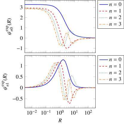
Figure 2: Radial parts of the exponential disc basis $\psi^{\text{exp}}_{nm}(r)$ for $n=0,1,2,3$ and $m=0$ (top) and $m=1$ (bottom). The potentials have been unit-normalised.

Some examples of the potential basis elements $\psi_{nm}^{\text{exp}}(R)$ are plotted in Fig. 2.

5 Numerical implementation

At the end of Sec. 2 we mentioned the main obstacles to the effective implementation of the new algorithm – primarily the numerical stability when computing the coefficients $\beta_{nl}$, but also the need to compute repeated radial derivatives of the zeroth-order elements.

For the recurrence coefficients $\beta_{nl}$ the difficulty is that naively computing the integrals (2.20) becomes computationally expensive very quickly with increasing order $n$ (and to some extent also with $l$). Therefore it is essential to pick a numerical integration method that is fast without sacrificing accuracy. Unfortunately due to the total freedom in choice of zeroth-order $\rho_{0l}$, it is difficult to find a quadrature scheme for the integrals (2.20) that is optimal in general.

Fortunately, due to the link to the polynomials $p_{nl}(s)$ developed in Sec. 3, we can take advantage of the extensive literature on the construction of general orthogonal polynomials. Following Gautschi (1985) we have two options: either the discretized Stieltjes procedure or the modified Chebyshev algorithm. As it happens, computing the recurrence coefficients naively as in (2.20) is directly analogous to using the discretized Stieltjes procedure, except that now we perform the integrals in Fourier-Mellin space. This turns out to be the better option numerically, as the modified Chebyshev algorithm runs into floating point issues sooner due to catastrophic cancellation of terms. However, for completeness we describe both algorithms (Sections 5.1 and 5.2). We also discuss computer-assisted techniques for performing the repeated differentiations (Sec. 5.3).

All these methods are illustrated throughout for a basis set constructed to have the isochrone model (Henon, 1959) as its zeroth-order, and we follow up the numerical discussion with a demonstration of the validity of the isochrone-adapted basis set (Sec. 5.4); however the underlying methods we describe are applicable to any suitable zeroth-order model. The potential, density and polynomial weight function for the isochrone model are as follows:

$$\Phi_{0l}^{\text{iso}}(r) =\frac{-r^{l}}{\left(1+\sqrt{1+r^{2}}\right)^{2l+1}},$$ (5.1)

$$\rho_{0l}^{\text{iso}}(r) =\frac{(2l+1)r^{l}\left[(2l+3)(1+\sqrt{1+r^{2}})+(2l+2)r^{2}\right]}{(1+\sqrt{1+r^{2}})^{2l+3}(1+r^{2})^{3/2}},$$

$$\omega_{l}^{\text{iso}}(s) =\frac{(2l+1)^{2}}{2^{2l+6}\pi^{2}}\left|\frac{\Gamma\!\left(l+3/2+\mathrm{i}s\right)\Gamma\!\left(l/2+1/4+\mathrm{i}s/2\right)}{\Gamma\!\left(3l/2+7/4+\mathrm{i}s/2\right)}\right|^{2}.$$

The precise $l$-dependence of these expressions is of course arbitrary to some extent, but we have made a suitable ‘natural’ choice.

5.1 Discretized Stieltjes procedure

The sequence of recurrence coefficients $\beta_{nl}$ that we need to compute can be expressed as the ratio of two integrals,

$$\beta_{nl}=\frac{I_{nl}}{I_{n-1,l}},\>\>\mathrm{where}\>\>I_{nl}=\langle\rho_{nl},\rho_{nl}\rangle=\lVert\rho_{nl}\rVert^{2},$$ (5.2)

and so for each higher $n$ we need one additional evaluation of $I_{nl}$. Evaluations of $\beta_{nl}$ alternate with applications of the recurrence relation (3.25) to find the next basis element $\rho_{nl}$. Once sufficient $\beta_{nl}$ have been found, the potential or density functions $\rho_{nlm}$ and $\Phi_{nlm}$ can be evaluated via their own recurrences as described in Sec. 2.

The difficulty then is in finding an appropriate strategy to compute the integrals $I_{nl}$. We opt to evaluate them in Fourier-Mellin-space, using the polynomials $p_{nl}(s)$ directly, and making use of the fact that the integral can be written

$$I_{nl}=\int_{-\infty}^{\infty}\omega_{l}(s)\left[p_{nl}(s)\right]^{2}ds.$$ (5.3)

Therefore the first step is to determine the weight function $\omega_{l}(s)$. This can be found in terms of the (Fourier-)Mellin transform of either the zeroth-order potential or the density,

$$\omega_{l}(s) =\frac{2K_{0l}^{2}}{(l+1/2)^{2}+s^{2}}\left|\mathcal{M}_{r}\!\left\{\rho_{0l}(r)\right\}\!\!\left(5/2+\mathrm{i}s\right)\right|^{2}$$ (5.4)

$$=\frac{(l+1/2)^{2}+s^{2}}{8\pi^{2}}\left|\mathcal{M}_{r}\left\{\Phi_{0l}(r)\right\}(1/2+\mathrm{i}s)\right|^{2}.$$

The Mellin transform is perhaps one of the less familiar integral transforms, but in practice a wide variety of Mellin transforms can be found in closed-form (helped especially by computer algebra systems), in part because with a logarithmic change of variable it can be written as a Fourier transform. All the polynomial weight functions considered in this paper can be found symbolically using Mathematica. Numerical evaluation of the Mellin transform is also an option – by transformation to the Fourier transform and approximation using Fast Fourier Transform methods – however we do not pursue this further in the present work.

Now we consider the asymptotic behaviour of the weight function $\omega_{l}(s)$ as $s\to\pm\infty$. The smoothness requirement (2.8) on $\rho_{0l}$ forces $\omega_{l}(s)$ to decay faster than any power of $s$, i.e. at least exponentially. We expect that

$$\omega_{l}(s)\sim|s|^{b}\>\mathrm{e}^{-a|s|}\>\>\mathrm{as}\>\>s\to\pm\infty,$$ (5.5)

so we need to determine the decay constant $a$. In the case of our isochrone basis set this asymptotic behaviour is derived from the behaviour of the complex gamma function at infinity (DLMF §5.11.9), giving $\omega_{l}(s)\sim\left|s\right|^{-1}\mathrm{e}^{-\pi\left|s\right|}$, or $a=\pi$. When $\omega_{l}(s)$ can be written down, it is usually simple to read off the decay constant $a$; for example, the double power-law basis sets (Sec. 4.1.2) have $a=\alpha$.

The at-least-exponential decay of the weight function suggests that the appropriate discretisation scheme for (5.3) is Gauss-Laguerre quadrature. To implement this for the isochrone case, rewrite (5.3) to pull out a factor of $\mathrm{e}^{-\pi s}$, and use the symmetry of the integrand to change the domain of integration to $(0,\infty)$ (defining $x=\pi s$),

$$I_{nl}=\frac{2}{\pi}\int_{0}^{\infty}\mathrm{e}^{-x}\>\underbrace{\mathrm{e}^{x}\>\omega_{l}(x/\pi)\>\left[p_{nl}(x/\pi)\right]^{2}}_{\sim x^{2n-1}\text{ as }x\to\infty}\>dx$$ (5.6)

We can then implement Gauss-Laguerre quadrature of order $\nu$, as a weighted sum over evaluation points $x_{j\nu}$, which are the roots of the $\nu$th Laguerre polynomial $L_{\nu}(x)$:

$$I_{nl}\approx\frac{2}{\pi}\sum_{j=1}^{\nu}w_{j\nu}\>\mathrm{e}^{x_{j\nu}}\>\omega_{l}(x_{j\nu}/\pi)\>\left[p_{nl}(x_{j\nu}/\pi)\right]^{2},$$ (5.7)

$$w_{j\nu}=\frac{x_{j\nu}}{\left[(\nu+1)\>L_{\nu+1}\left(x_{j\nu}\right)\right]^{2}},$$

$$L_{\nu}\!\left(x_{j\nu}\right)=0,\qquad j=1\ldots\nu.$$

The quadrature rule of order $\nu$ integrates polynomials exactly up to order $2\nu-1$, so to compute $I_{nl}$ with the isochrone weight function we would expect to need at least $\nu\geq n$. (An acceptable rule of thumb is that $I_{nl}$ requires $\nu=\text{max}(n+l,10)$.) It may be necessary to compute the weights $w_{j\nu}$ and roots $x_{j\nu}$ to a higher order of precision internally using arbitrary-precision arithmetic, but this is not a bottleneck in practice – and typically Gauss-Laguerre quadrature is implemented as a library function whose implementation details are hidden. In this way we can get e.g. $50$ orders of $\beta_{nl}$ to floating-point precision in under a tenth of a second using one core of a modern CPU.

The radial parts of some examples of potential elements in the isochrone basis set are plotted in Fig. 1.

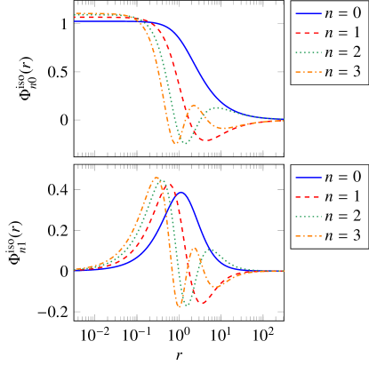
Figure 1: Radial parts of the isochrone potential basis $\Phi^{\text{iso}}_{nl}(r)$ for $n=0,1,2,3$ and $l=0$ (top) and $l=1$ (bottom). The potentials have been unit-normalised.

5.2 Modified Chebyshev algorithm

This is an alternative method described in Gautschi (1985), which we find to be less numerically stable in practice. However we describe it here for completeness, as it may yet find some usefulness (e.g. to facilitate finding exact expressions for the recurrence coefficients in certain cases).

Gautschi’s modified Chebyshev algorithm prescribes the modified moments

$${\tilde{\mu}}_{kl}\equiv\int_{-\infty}^{\infty}\omega_{l}(s)\>{\tilde{p}}_{kl}(s).$$ (5.8)

Here, ${\tilde{p}}_{kl}(s)$ are some auxiliary set of (monic) polynomials, orthogonal with respect to a symmetric measure on the interval $(-\infty,\infty)$, and obeying a three-term recurrence relation

$${\tilde{p}}_{-1,l}(s) =0,$$ (5.9)

$${\tilde{p}}_{k+1,l}(s) =s\>{\tilde{p}}_{kl}(s)-{\tilde{\beta}}_{kl}{\tilde{p}}_{k-1,l}(s).$$

By symmetry this means that ${\tilde{\mu}}_{kl}$ are nonzero only for even $k$. In principle the choice of auxiliary polynomial is wide open, but the obvious choice in our case (for ease and stability of computation) is the monic Hermite polynomials $H\!e_{k}(s)$, for which ${\tilde{\beta}}_{kl}=k$. We can then proceed to find the mixed moments

$$\sigma_{jkl}=\int_{-\infty}^{\infty}p_{jl}(s)\>{\tilde{p}}_{kl}(s)\>\omega_{l}(s)\>ds$$ (5.10)

via a system of recurrence relations that produces the desired recurrence coefficients $\beta_{nl}$ as a byproduct:

$$\sigma_{0kl} ={\tilde{\mu}}_{kl},$$ (5.11)

$$\sigma_{jkl} =\sigma_{j-1,k+1,l}-\beta_{j-1,l}\sigma_{j-2,k,l}+{\tilde{\beta}}_{kl}\sigma_{j-1,k-1,l},$$

$$\beta_{nl} =\frac{\sigma_{nnl}}{\sigma_{n-1,n-1,l}}.$$

In practice (for our isochrone basis set) we find that $\sigma_{jkl}$ suffers from catastrophic cancellation beyond approximately $j=20$. Alternatively if the modified moments ${\tilde{\mu}}_{kl}$ are known in ‘closed-form’ then this method is convenient for finding ‘exact’ recurrence coefficients. This turns out to be the case for the isochrone basis set, for which see App. G.

5.3 Repeated differentiation

There are three classes of algorithm for computer-assisted differentiation: 1. finite-differencing, 2. symbolic differentiation, and 3. automatic differentiation. The first of these we can discount pretty much immediately as being wildly numerically unstable and expensive compared to the other two.

The second, symbolic differentiation via computer algebra, is potentially competitive at low expansion orders, but it is hard to predict the degree of blow-up in the number of algebraic terms. It depends strongly on the precise form of the function that is being differentiated. In practice we find that efficient application of symbolic differentiation at high expansion orders requires alternating between differentiation and algebraic simplification.

Of course, one may also attempt symbolic differentiation by hand, attempting to find simplifications that reduce the tower of applications of $\mathcal{D}^{n}$ to a simpler form – whether this is possible also depends on the form of $\Phi_{0l}$ and $\rho_{0l}$. Many of the basis sets considered in Sec. 4 have simple closed-forms (at all orders) due to fortunate simplification in repeated differentiation. For example, taking the double-power law basis (Sec. 4.1.2) with parameters $\alpha=1/2$, $\nu=p-3/2$ and $n=l=0$ (and labelling each density function with $p$), we have

$$\rho_{p+1}=p^{-1}\>(p-5/4-\mathrm{i}\mathcal{D}/2)\rho_{p}.$$ (5.12)

Using this identity in (4.8) then leads (after some further simplification) to a known closed-form expression for $\rho_{nl}^{\text{LSE}}$. However it is likely to be difficult to find easy differentiation formulas in general. For our isochrone basis set, the method we give in App. G for computing the modified moments can be adapted to find expressions for the higher-order derivatives, but the result is complicated and of dubious numerical stability.

The third method, automatic differentiation (AD) is what we find to be most competitive in practice. This is a general term referring to a class of algorithms implemented entirely at the software library level, that provides an evaluation of the derivative at a single point given only knowledge of the chain rule and the differentiation rules for primitive arithmetic operations and standard mathematical library functions. Essentially, the function to be differentiated is written in ordinary code, and the AD algorithm automatically deduces the correct sequence of chain rule steps to carry out. For our purposes we require higher-order derivatives; while applying an AD algorithm to itself works in principle (and often works in practice) it is very inefficient, as the AD logic itself must be differentiated. It is better to use an AD implementation that natively understands higher-order derivatives.

As we are coding in the Julia programming language, we use a suitable library called TaylorSeries.jl (Benet & Sanders, 2019). A special variable $t(N)$ is instantiated that represents the first $N$ terms of an (abstract) Taylor series. Given a point $r_{0}$, we can use $t+r_{0}$ as the argument of any ordinary mathematical function; the result is the first $N$ coefficients of the Taylor series around $r_{0}$ that approximates that function. For example, setting $N=3$ and $r_{0}=1.0$ and using the potential of the isochrone model (5.1) as our function, the computer prints a data structure representing the following truncated Taylor series,

$$\Phi_{00}^{\text{iso}}(t(3)+1.0)=-0.4142+0.1213t-0.0052t^{2}-0.0225t^{3}.$$ (5.13)

When it comes to the actual implementation, we have two choices, which we find to have similar efficiency in practice. The first option begins with computing the vector of derivatives (at a point $\mathbf{r}_{0}$) up to some maximum order $N$ all in one go,

$$\mathbf{V}_{l}=(\Phi_{0lm},\mathcal{D}\Phi_{0lm},\mathcal{D}^{2}\Phi_{0lm},\ldots,\mathcal{D}^{N}\Phi_{0lm}).$$ (5.14)

In fact, because $\mathcal{D}$ can be expressed as a single differentiation with respect to a transformed variable (via $r\>d/dr=d/ds$, where $s=\log r$), $\mathbf{V}_{l}$ can be obtained directly from a single $N$-term Taylor series evaluation. Separately, we derive from $\beta_{nl}$ the matrix elements $(\mathsf{A}_{l})_{nj}=A_{njl}$ in the expansion

$$\Phi_{nlm}=\sum_{j=0}^{n}A_{njl}\>\mathcal{D}^{j}\Phi_{0lm}.$$ (5.15)

To evaluate a vector of potential functions at a single point,

$$\mathbf{\Phi}_{l}=(\Phi_{0lm},\Phi_{1lm},\ldots,\Phi_{Nlm})$$ (5.16)

we perform the contraction $\mathbf{\Phi}_{l}=\mathsf{A}_{l}\cdot\mathbf{V}_{l}$. At each different point $\mathbf{r}_{1}$, we have to re-compute $\mathbf{V}$ but not $\mathsf{A}$.

The second option is to use the recurrence relation directly (i.e. (2.18) or (2.19)). Because we know ahead of time that we want $N$ iterations of the recurrence relation, we set up the Taylor series $t(N)$, and use $r_{0}+t(N)$ as the dependent variable. The length of the series then shrinks as we go up the ladder of basis function evaluations. In practice this second method seems to be marginally slower than the first one, as more operations on the abstract Taylor series need to be performed.

5.4 Unstable modes of a spherical system

It is important to check whether a basis set constructed according to the prescriptions of Sec. 5 actually works in practice. One simple approach might be to just construct $n$ basis functions, and integrate up the $n\times n$ square of inner products, testing whether orthogonality is achieved to a given floating-point precision. However, we know that it is possible to construct basis sets that are genuinely orthogonal but whose expansions of realistic mass densities fail to converge in practice, or display other undesirable numerical effects. Therefore we choose to demonstrate the validity of our approach by reproducing a physical result from the literature – the unstable radial mode of the isochrone model.

We use the discretized Stieltjes method described in Sec. 5.1, where the basis set is adapted to the isochrone model at zeroth order. However the specific adaptation is not the crucial part; for this particular application only the perturbing density needs to be accurately resolved by the basis elements, so the key feature required of the basis set is only that it has the correct asymptotic behaviour. To this end, we adapt the code and method of Fouvry & Prunet (2022) to show that the same unstable mode is recovered by our isochrone-adapted basis set. The part of the code that implements the basis set may be found at https://github.com/ejlilley/basis.

The details of the computation can be found in Fouvry & Prunet (2022). In brief, we start with knowledge of an isotropic distribution function that solves the collisionless Boltzmann equation for the isochrone potential. We also have the corresponding action and angle coordinates $(\mathbf{J},\mathbf{w})$ as a function of position and momentum, which for the isochrone potential are known in closed form. Then, each potential basis element must be Fourier-transformed with respect to the angle coordinates

$${\hat{\Phi}}_{nlm}^{\mathbf{n}}(\mathbf{J})=(2\pi)^{-3}\int\!d^{\,3}\!\mathbf{w}\>\mathrm{e}^{-\mathrm{i}\mathbf{n}\cdot\mathbf{w}}\>\Phi_{nlm}(\mathbf{J},\mathbf{w}),$$ (5.17)

out of which a matrix $\mathsf{M}$ is formed,

$$(\mathsf{M})_{n_{1}l_{1},n_{2}l_{2}}=(2\pi)^{3}\sum_{\mathbf{n}}\int\!d^{\,3}\!\mathbf{J}\>{\hat{\Phi}}_{n_{1}l_{1}0}^{\mathbf{n}}\>\overline{{\hat{\Phi}}_{n_{2}l_{2}0}^{\mathbf{n}}}\>R_{\mathbf{n}}(s),$$ (5.18)

where the $R_{\mathbf{n}}(s)$ represents the collisionless Boltzmann operator for a perturbation with growth rate proportional to $\mathrm{e}^{st}$. The unstable growing mode then corresponds to a solution $\mathbf{A}$ of the matrix equation

$$(\mathsf{M}+\mathbb{I})\cdot\mathbf{A}=0,$$ (5.19)

with the vector of coefficients $\mathbf{A}=\left(A_{nl}\right)$ giving the expansion of the mode $\delta\Phi$ with respect to the basis $\{\Phi_{nlm}\}$,

$$\delta\Phi=\sum_{nl}A_{nl}\>\Phi_{nl0}.$$ (5.20)

A plot of this mode is shown in Fig. 3. The maximum expansion orders were $n_{\mathrm{max}}=6$ and $l_{\mathrm{max}}=2$, with a scale length of $r_{s}=1$ and a maximum resonance number of $n_{1}^{\mathrm{max}}=10$. All our other integration parameters are identical to those in Fouvry & Prunet (2022, App. C), where a matching result was obtained using the Clutton-Brock (1973) basis set with $n_{\mathrm{max}}=100$ and $r_{s}=20$ – the mode shape also agreeing with the original result of Saha (1991). As mentioned previously, it is not strictly necessary to exactly match the zeroth-order element of the basis set to the underlying equilibrium model. However the basis elements must have the correct asymptotic behaviour, so using the isochrone-adapted basis set guarantees that this condition is satisfied. Nevertheless, our results do hint that accurate mode recovery may be possible with many fewer basis elements when the basis is suitably adapted, although we hesitate to draw any firm conclusions until a more systematic comparison can be drawn.

Calculating the matrix $\mathsf{M}$ is very computationally expensive, as it requires multiple truncated infinite summations, over several indices ($n$, $l$ and the vector of wavenumbers $\mathbf{n}$). It also requires two nested integrations, as the Fourier transform (5.17) must also be performed numerically. In the general non-isochrone case a third level of integration is required, because the action and angle coordinates are no longer known in closed-form. Any method of reducing this computational effort is therefore desirable. It is possible that judicious choice of basis elements and application of their differential-recursion relation (2.19) may ameliorate these calculations, but further investigation is needed.

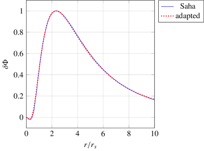
Figure 3: Recovery of the unstable radial mode of the isotropic isochrone model. The mode is recovered well despite the low ($n_{\mathrm{max}}=6$) number of basis functions used.

6 Discussion and Conclusions

We have reformulated the study of bi-orthogonal basis sets using the language of Fourier-Mellin transforms. This unexpected development unifies many previous results into a coherent theoretical framework. The general idea of generating new potential-density pairs from old by differentiation is not entirely new. Traditionally this is accomplished by differentiating with respect to the model’s scalelength – in particular, Aoki & Iye (1978) found compact expressions for Clutton-Brock (1972)’s thin disc basis by repeatedly applying the operator $a\partial_{a}$ (for $a$ the scalelength) and orthogonalising the resulting sequence of potential-densities by the Gram-Schmidt process. Subsequently de Zeeuw & Pfenniger (1988), in the course of deriving a series of ellipsoidal potential-density pairs, noted that the operators $r\partial_{r}$ and $\nabla^{2}$ obey an important commutation relation (which we re-derive in App. B). Therefore Aoki & Iye (1978)’s result (and by extension our algorithm presented here) can be expressed in terms of the coordinates alone, without reference to an arbitrary scalelength.

The formalism developed in sections 2–3 deserves some further interpretation. In particular, the operator $\mathcal{D}$ on which the whole development hinges may appear to have been plucked out of thin air, but it is in fact no accident: $\mathcal{D}$ is precisely the infinitesimal generator of the scaling symmetry of the self-energy inner product (2.1). To briefly motivate this, let $S_{t}$ be a ‘radial scaling’ operator,

$$(S_{t}f)(\mathbf{r})=t^{-5/2}f(t\mathbf{r}).$$ (6.1)

As is immediately evident from dimensional analysis, this preserves the self-energy, i.e.

$$\langle S_{t}f,S_{t}g\rangle=\langle f,g\rangle.$$ (6.2)

The operator $\mathcal{D}$ is now defined in terms of the infinitesimal generator of $S_{t}$,

$$(\mathcal{D}f)(\mathbf{r})\equiv\mathrm{i}\left.\frac{d}{dt}(S_{t}f)(\mathbf{r})\right|_{t=0}.$$ (6.3)

Differentiating (6.2) with respect to the parameter $t$, it is immediately evident that $\mathcal{D}$ is self-adjoint. In Sec. 3.1 we implicitly invoked Stone’s theorem from functional analysis to provide a Fourier-like transform whose integral kernel is the eigenfunction of a self-adjoint operator. In our case the operator is $\mathcal{D}$, the eigenfunction is $\Psi_{s}$ (3.2), and the resulting integral transform is exactly the radial part of the Fourier-Mellin transform that we defined in (3.4). The spherical harmonics arise from a similar argument applied to the generators of the coordinate rotations.

This line of reasoning suggests that it may be worthwhile to look for other symmetries of the self-energy inner product, perhaps arising from other coordinate systems or geometries in which the Laplacian separates. Given a set of three mutually-commuting operators arising from three symmetries of the self-energy, we would expect to be able to construct a basis set formalism similar to that of the present work. To sketch out what this looks like in full generality, let $\tau$ be a suitable self-adjoint operator according to the criteria just described (restricting to one spatial dimension for the sake of discussion). Then the self-adjointness condition (2.6) combined with the properties of the inner product (2.1) implies that

$$\nabla^{2}\tau=\tau^{*}\nabla^{2},$$ (6.4)

where $\tau^{*}$ is the Hermitian adjoint of $\tau$ with respect to the ordinary inner product on $L^{2}$ functions (A.3). Suppose further that we have found a set of orthogonal potential functions $\{\Phi_{n}\}$, with an index-raising polynomial $p_{n}(s)$ such that

$$\Phi_{n}=p_{n}(\tau)\Phi_{0}.$$ (6.5)

Then the associated density functions (obeying $\nabla^{2}\Phi_{n}=\rho_{n}$) are given by

$$\rho_{n}=p_{n}(\tau^{*})\rho_{0}.$$ (6.6)

There are further simplifications involved in Sec. 3, which come about essentially because $\mathcal{D}=\mathcal{D}^{*}+\text{const.}$, which means that the eigenfunctions of $\mathcal{D}$ and $\mathcal{D}^{*}$ are the same up to a constant shift in the eigenvalue. Generically we would expect a different relationship between $\tau$ and $\tau^{*}$.

The task remaining, which we leave to future efforts, is therefore to classify the symmetries of the self-energy inner product, in order to develop expansions that are usefully adapted to different coordinate systems and geometries. In a sense, the ‘holy grail’ would be the construction of an expansion adapted to the confocal ellipsoidal coordinate system, appropriate for studying the equilibrium dynamics of ellipsoidal galaxies.

Some symmetries are already known. For example, in Cartesian coordinates $(x,y,z)$ we trivially have the three cardinal translations ($x\mapsto x+a$ etc.). Writing down their associated infinitesimal generators $X=\mathrm{i}\partial_{x}$, $Y=\mathrm{i}\partial_{y}$ and $Z=\mathrm{i}\partial_{z}$, their joint eigenfunction $\mathrm{e}^{\mathrm{i}\mathbf{k}\cdot\mathbf{r}}$ is just the kernel of the standard Fourier transform, with the wavevector $\mathbf{k}$ taking the role of the (continuous) eigenvalue. The Fourier transform would therefore play the same role in the resulting basis set formalism as the Fourier-Mellin transform did in ours (Sec. 3). Poisson solvers directly using the Fourier transform are ubiquitous in astrophysical applications, so it would be interesting to construct a set of ‘Cartesian’ basis functions and compare their performance with the current state-of-the art.

Other symmetries are known from classical potential theory. Firstly, the Kelvin transform, which is an inversion in a sphere and preserves the self-energy up to a sign (Kalnajs, 1976). However it is not a continuous symmetry, so there is no associated infinitesimal self-adjoint operator. Secondly, a symmetry that takes spheres to concentric ellipsoids (sometimes called homeoids). This maps the spherical radius to an ‘ellipsoidal’ radius, $r\mapsto m=\sqrt{x^{2}/a^{2}+y^{2}/b^{2}+z^{2}/c^{2}}$. It has long been known that this transformation preserves the mutual self-energy of any two charge or mass densities (Carlson, 1961), up to a constant factor that is essentially just an elliptical integral of the three semi-axes $(a,b,c)$. We can use this to transform any purely spherical basis set into one stratified on concentric ellipsoids. Note however that the concentric ellipsoids in this transformation are distinct from the confocal ellipsoids inherent in the ellipsoidal coordinate system that is more dynamically relevant due to its relationship to the Stäckel potentials (de Zeeuw, 1985; de Zeeuw et al., 1986).

Also, we mention some gaps in our analysis. While we purport in this work to provide a general theory of orthogonal basis sets, there are some aspects that are still not fully characterised. Firstly, it is clear from Sec. 4 that there exists a connection between basis sets which have a classical index-raising polynomial $P_{n}(s)$, and those whose potential and density elements are known in closed-form (i.e. possessing a recurrence relation independent of $\mathcal{D}$ or $\mathcal{A}$). However, the exact nature of this connection is unknown, although it is likely related to the fact that the Hahn-type polynomials appearing in the various index-raising polynomials obey second-order difference equations. Secondly, we do not touch on the issue of basis sets appropriate for finite-radius systems. This was approached by Kalnajs (1976) in the case of thin discs, using a formalism initially similar to our own. There are also contributions from Polyachenko & Shukhman (1981) for finite spheres, and Tremaine (1976) for finite elliptical discs. In general it appears to be straightforward to construct basis sets for finite systems out of polynomials or Bessel functions, but a concrete connection to our new formalism would be attractive. A more rigorous form of the argument about completeness in Sec. 3.3 would also be desirable, as would a quantitative comparison with basis sets computed via the Sturm-Liouville approach of Weinberg (1999).

Finally, some broader speculation. It is possible that the general ideas developed here may find applications beyond the solution of Poisson’s equation. In physics we are often required to compute the inverse of Hermitian operators with a continuous spectrum – a well-known example being the Schrödinger operator for certain boundary conditions and choices of potential. These operators could conceivably be supplied with a set of (adapted) orthogonal basis functions, by identifying a suitable commuting set of self-adjoint operators and then diagonalising their cyclic vectors. Any such basis set then provides an infinite series representation of the Green’s function of the underlying Hermitian operator where the coordinates appear multiplicatively separated in each term. Such series representations may find use in various applications. The appearance of tridiagonal Jacobi operators in particular may presage links to similar numerical methods in quantum mechanics (Alhaidari et al., 2008; Ismail & Koelink, 2011).

Appendix A Self-adjointness of $\mathcal{D}$

Let $f,g$ be densities that are non-zero on a $\delta$-dimensional hyperplane in three-dimensional space ($\delta\leq 3$). Then

$$\langle f,g\rangle=\int d^{\delta}\mathbf{r}\int d^{\delta}\mathbf{r}^{\prime}f(\mathbf{r})\overline{g(\mathbf{r}^{\prime})}\,G(\mathbf{r},\mathbf{r}^{\prime}),$$ (A.1)

where the (three-dimensional Newtonian) Green’s function $G$ is

$$G(\mathbf{r},\mathbf{r}^{\prime})=\lVert\mathbf{r}-\mathbf{r}^{\prime}\rVert^{-1}=\left(r^{2}+r^{\prime 2}-2rr^{\prime}\cos{\phi}\right)^{-1/2},$$ (A.2)

and $\phi$ is the angle between the two position vectors. Also define the ordinary $L^{2}$ inner product,

$$(f,g)=\int d^{\delta}\mathbf{r}f(\mathbf{r})\overline{g(\mathbf{r})}.$$ (A.3)

We write $\theta=r\partial_{r}$ and $\theta^{\prime}=r^{\prime}\partial_{r^{\prime}}$. Preliminaries: first note that

$$(\theta+\theta^{\prime})G=-G,$$ (A.4)

and also note that (from integration by parts on $r$)

$$(f,\theta g)+(\theta f,g)=-\delta(f,g).$$ (A.5)

So we compute

$$\langle f,\theta g\rangle =\int d^{\delta}\mathbf{r}\int d^{\delta}\mathbf{r}^{\prime}f(\mathbf{r})G(\mathbf{r},\mathbf{r}^{\prime})\theta^{\prime}\,\overline{g(\mathbf{r}^{\prime})}$$ (A.6)

$$=-\int d^{\delta}\mathbf{r}\int d^{\delta}\mathbf{r}^{\prime}\left[f(\mathbf{r})(\delta G(\mathbf{r},\mathbf{r}^{\prime})\overline{g(\mathbf{r}^{\prime})}+\overline{g(\mathbf{r}^{\prime})}\,\theta^{\prime}G(\mathbf{r},\mathbf{r}^{\prime})\right]$$

$$=\int d^{\delta}\mathbf{r}\int d^{\delta}\mathbf{r}^{\prime}\left[(1-\delta)f(\mathbf{r})G(\mathbf{r},\mathbf{r}^{\prime})\overline{g(\mathbf{r}^{\prime})}+f(\mathbf{r})\overline{g(\mathbf{r}^{\prime})}\,\theta G(\mathbf{r},\mathbf{r}^{\prime})\right]$$

$$=\int d^{\delta}\mathbf{r}\int d^{\delta}\mathbf{r}^{\prime}\left[(1-2\delta)f(\mathbf{r})G(\mathbf{r},\mathbf{r}^{\prime})\overline{g(\mathbf{r}^{\prime})}-\overline{g(\mathbf{r}^{\prime})}G(\mathbf{r},\mathbf{r}^{\prime})\,\theta f(\mathbf{r})\right]$$

$$=(1-2\delta)\langle f,g\rangle-\langle\theta f,g\rangle,$$

where to obtain the final result we applied (A.5), then (A.4), and then (A.5) again. So define $\mathcal{D}$ in a $\delta$-dependent way, as

$$\mathcal{D}=\mathrm{i}(\theta+\delta-1/2),$$ (A.7)

and we can see that

$$\langle f,\mathcal{D}g\rangle=\langle\mathcal{D}f,g\rangle.$$ (A.8)

Setting $\delta=3$ (i.e. no restriction to a hyperplane) gives the appropriate result for spherical geometry. For thin discs we have $\mathcal{A}=\left.\mathcal{D}\right|_{\delta=2}$. We could also consider $\delta=1$ for an infinite line density.

Appendix B Commutator of $\mathcal{D}$ and $\nabla^{2}$

Working on a $\delta$-dimensional hyperplane again, write the potential using the Green’s function (A.2),

$$\Phi(\mathbf{r})=\int d^{\delta}\mathbf{r}^{\prime}\rho(\mathbf{r}^{\prime})G(\mathbf{r},\mathbf{r}^{\prime}).$$ (B.1)

Now apply $\theta$, giving

$$\theta\Phi(\mathbf{r}) =\int d^{\delta}\mathbf{r}^{\prime}\rho(\mathbf{r}^{\prime})\left[G(\mathbf{r},\mathbf{r}^{\prime})+\theta^{\prime}G(\mathbf{r},\mathbf{r}^{\prime})\right]$$ (B.2)

$$=-\Phi(\mathbf{r})+\int d^{\delta}\mathbf{r}^{\prime}G(\mathbf{r},\mathbf{r}^{\prime})\left(\delta+\theta^{\prime}\right)\rho(\mathbf{r}^{\prime})$$

$$=(\delta-1)\Phi(\mathbf{r})+\int d^{\delta}\mathbf{r}^{\prime}G(\mathbf{r},\mathbf{r}^{\prime})\theta^{\prime}\rho(\mathbf{r}^{\prime}),$$

where we used (A.4) and then (A.5). Note that in the spherical ($\delta=3$) case this is equivalent to calculating the following commutator,

$$[\nabla^{2}_{l},\theta]=\nabla^{2}_{l}\theta-\theta\nabla^{2}_{l}=2\nabla^{2}_{l},$$ (B.3)

which can be shown directly by differentiation and the Leibniz rule; however (B.3) is inapplicable to the thin disc ($\delta=2$) case, so the previous derivation in terms of the Green’s function is required. Now, writing these results in terms of the self-adjoint operator $\mathcal{D}$, we have

$$\left(\mathcal{D}+(1-\delta)\mathrm{i}\right)\Phi=\int d^{\delta}\mathbf{r}^{\prime}G(\mathbf{r},\mathbf{r}^{\prime})\mathcal{D}^{\prime}\rho(\mathbf{r}^{\prime}).$$ (B.4)

Specialising to the spherical case, if for some basis set $\{\rho_{n}\}$ there exists a suitable index-raising polynomial $P_{n}(s)$, we have

$$\rho_{n}=P_{n}(\mathcal{D})\rho_{0}$$ (B.5)

for the density functions, and

$$\Phi_{n}=P_{n}\!\left(\mathcal{D}-2\mathrm{i}\right)\Phi_{0}$$ (B.6)

for the potentials. Analogously, in the thin disc case, we have

$$\sigma_{n}=P_{n}(\mathcal{A})\sigma_{0}$$ (B.7)

and

$$\psi_{n}=P_{n}\!\left(\mathcal{A}-\mathrm{i}\right)\psi_{0}.$$ (B.8)

Appendix C The Fourier-Mellin transform

We develop expressions for the forwards and reverse Fourier-Mellin transform, and the corresponding orthogonality relation. A similar procedure is followed for both the spherical and the thin disc cases.

C.1 Spherical case

We work in spherical polar coordinates $(r,\vartheta,\varphi)$, with $\mathbf{r}=r\hat{\mathbf{r}}$. Our density basis function for the Fourier-Mellin transform is $\Psi_{slm}$, defined in (3.3). The corresponding potential, obeying $\nabla^{2}\phi_{slm}=4\pi\Psi_{slm}$, is

$$\phi_{slm}(\mathbf{r})=\frac{-4\pi}{K_{l}(\mathrm{i}s)}\>r^{-\mathrm{i}s-1/2}\>Y_{lm}(\hat{\mathbf{r}}),$$ (C.1)

where $K_{l}(\mathrm{i}s)$ is defined in (3.5). The expansion of an arbitrary mass density $F$ with respect to the $\Psi_{slm}$-basis is the Fourier-Mellin transform of $F$:

$$\langle F,\Psi_{slm}\rangle =-\int\!d^{3\,}\!\mathbf{r}\>F(\mathbf{r})\>\overline{\phi_{slm}(\mathbf{r})}$$ (C.2)

$$=\frac{4\pi}{K_{l}(\mathrm{i}s)}\int_{0}^{\infty}r^{2}dr\>r^{\mathrm{i}s-1/2}\int\!d^{2}\hat{\mathbf{r}}\>\overline{Y_{lm}(\hat{\mathbf{r}})}\>F(\mathbf{r})$$

$$=\frac{4\pi}{K_{l}(\mathrm{i}s)}\mathcal{M}_{r}\!\left\{F_{lm}(r)\right\}\!\!\left(5/2+\mathrm{i}s\right),$$

where $F_{lm}(r)=\int\!d^{2}\hat{\mathbf{r}}\>\overline{Y_{lm}(\hat{\mathbf{r}})}\>F(\mathbf{r})$ are the spherical multipole moments of $F$. Inverting this using the Mellin inversion theorem (3.8) (choosing the constant $c=5/2$ in the integral), we have

$$F(\mathbf{r})=\frac{1}{8\pi^{2}}\sum_{lm}\int_{-\infty}^{\infty}ds\>K_{l}(\mathrm{i}s)\>\Psi_{slm}(\mathbf{r})\>\langle F,\Psi_{slm}\rangle.$$ (C.3)

The potential corresponding to the density $F$ can be expressed similarly by replacing $\Psi_{slm}(\mathbf{r})$ in (C.3) by its potential $\phi_{slm}(\mathbf{r})$. Finally, the mutual energy of two densities $F_{1}$ and $F_{2}$ is

$$\langle F_{1},F_{2}\rangle=\frac{1}{8\pi^{2}}\sum_{lm}\int_{-\infty}^{\infty}ds\>K_{l}(\mathrm{i}s)\>\langle F_{1},\Psi_{slm}\rangle\>\langle\Psi_{slm},F_{2}\rangle$$ (C.4)

and the Fourier-Mellin basis functions satisfy the orthogonality relation

$$\langle\Psi_{slm},\Psi_{t\lambda\mu}\rangle=\frac{8\pi^{2}}{K_{l}(\mathrm{i}s)}\>\delta_{m\mu}\>\delta_{l\lambda}\>\delta(s-t).$$ (C.5)

C.2 Disc case

We work in cylindrical polar coordinates $(R,\varphi,z)$, with $\mathbf{R}=R\hat{\mathbf{R}}$. Define $\mathcal{A}=\mathrm{i}(R\partial_{R}+3/2)$. Then for two arbitrary thin disc densities $\sigma_{1},\sigma_{2}\propto\delta(z)$ we have $\langle\mathcal{A}\sigma_{1},\sigma_{2}\rangle=\langle\sigma_{1},\mathcal{A}\sigma_{2}\rangle$, i.e. $\mathcal{A}$ is self-adjoint (see App. A for proof, setting $\delta=2$ at the end to give the thin disc case). The eigenfunctions of $\mathcal{A}$ are $\Sigma_{s}(R)=R^{-\mathrm{i}s-3/2}$ with real eigenvalue $s$. We then adjoin a cylindrical harmonic to form the basis functions (Kalnajs’ logarithmic spirals)

$$\Sigma_{sm}(\mathbf{R})=\Sigma_{s}(R)\>\mathrm{e}^{\mathrm{i}m\varphi}=R^{-\mathrm{i}s-3/2}\>\mathrm{e}^{\mathrm{i}m\varphi}.$$ (C.6)

Using Toomre’s Hankel-transform method we can find the potential corresponding to this density, which is

$$\psi_{sm}(R,\varphi,0)=\frac{-\pi}{K_{m}(\mathrm{i}s)}\>R^{-\mathrm{i}s-1/2}\>\mathrm{e}^{\mathrm{i}m\varphi},\qquad K_{m}(\mathrm{i}s)=\left|\frac{\Gamma\!\left(\frac{m+3/2+\mathrm{i}s}{2}\right)}{\Gamma\!\left(\frac{m+1/2+\mathrm{i}s}{2}\right)}\right|^{2}\geq 0,$$ (C.7)

so that in the plane (i.e. first acting with the full Laplacian, then afterwards setting $z=0$) we have

$$\left.\nabla^{2}\psi_{sm}(\mathbf{r})\right|_{z=0}=4\pi\Sigma_{sm}(\mathbf{R}).$$ (C.8)

Now we compute the thin disc Fourier-Mellin transform for an arbitrary thin disc density $\sigma$,

$$\langle\sigma,\Sigma_{sm}\rangle =-\int\!d^{3\,}\!\mathbf{r}\>\sigma(\mathbf{R})\>\delta(z)\>\overline{\psi_{sm}(\mathbf{r})}$$ (C.9)

$$=\frac{\pi}{K_{m}(\mathrm{i}s)}\int_{0}^{\infty}R\>dR\>R^{\mathrm{i}s-1/2}\int_{0}^{2\pi}d\phi\>\mathrm{e}^{-\mathrm{i}m\varphi}\sigma(\mathbf{R})$$

$$=\frac{\pi}{K_{m}(\mathrm{i}s)}\mathcal{M}_{R}\!\left\{\sigma_{m}(R)\right\}\!\!\left(3/2+\mathrm{i}s\right),$$

where $\sigma_{m}(R)$ are the cylindrical multipoles of $\sigma(\mathbf{R})$. Using the Mellin inversion theorem to invert this transform (3.8) (with constant $c=3/2$) gives

$$\sigma(\mathbf{R})=\frac{1}{4\pi^{3}}\sum_{m=-\infty}^{\infty}\int_{-\infty}^{\infty}ds\>K_{m}(\mathrm{i}s)\>\Sigma_{sm}(\mathbf{R})\>\langle\sigma,\Sigma_{sm}\rangle.$$ (C.10)

Therefore the mutual energy of two thin disc densities can be expressed as

$$\langle\sigma_{1},\sigma_{2}\rangle=\frac{1}{4\pi^{3}}\sum_{m=-\infty}^{\infty}\int_{-\infty}^{\infty}ds\>K_{m}(\mathrm{i}s)\>\langle\sigma_{1},\Sigma_{sm}\rangle\>\langle\Sigma_{sm},\sigma_{2}\rangle.$$ (C.11)

We also have the orthogonality relation

$$\langle\Sigma_{sm},\Sigma_{t\mu}\rangle=\frac{4\pi^{3}}{K_{m}(\mathrm{i}s)}\>\delta_{m\mu}\>\delta(t-s).$$ (C.12)

As noted in Sec. 3.2.3, these results are independent of the $z$-dependence of the potential away from the disc plane.

Appendix D Orthogonality relation

D.1 Spherical case

For the inner product of any two density basis functions $\rho_{nlm}$ we have

$$\langle\rho_{nlm},\rho_{n^{\prime}l^{\prime}m^{\prime}}\rangle =\frac{\delta_{ll^{\prime}}\delta_{mm^{\prime}}}{8\pi^{2}}\int_{-\infty}^{\infty}ds\>K_{l}(\mathrm{i}s)\>\langle\Psi_{slm},\rho_{nlm}\rangle\>\langle\rho_{n^{\prime}lm},\Psi_{slm}\rangle$$ (D.1)

$$=\frac{\delta_{ll^{\prime}}\delta_{mm^{\prime}}}{8\pi^{2}}\int_{-\infty}^{\infty}ds\>K_{l}(\mathrm{i}s)\>\langle\Psi_{slm},P_{nl}(\mathcal{D})\rho_{0lm}\rangle\>\langle P_{n^{\prime}l}(\mathcal{D})\rho_{0lm},\Psi_{slm}\rangle$$

$$=\frac{\delta_{ll^{\prime}}\delta_{mm^{\prime}}}{8\pi^{2}}\int_{-\infty}^{\infty}ds\>K_{l}(\mathrm{i}s)\>\overline{P_{nl}(s)}\>P_{n^{\prime}l}(s)\left|\langle\Psi_{slm},\rho_{0lm}\rangle\right|^{2}.$$

The non-polynomial factors in the above expression are collected into a weight function $\omega_{l}(s)$, which can be written explicitly in terms of the Mellin transform of the zeroth-order density (or a similar expression in terms of the zeroth-order potential – see (5.4)),

$$\omega_{l}(s) =\frac{K_{l}(\mathrm{i}s)}{8\pi^{2}}\left|\langle\rho_{0lm},\Psi_{slm}\rangle\right|^{2}$$ (D.2)

$$=\frac{2K_{0l}^{2}}{K_{l}(\mathrm{i}s)}\left|\mathcal{M}_{r}\!\left\{\rho_{0l}(r)\right\}\!\!\left(5/2+\mathrm{i}s\right)\right|^{2}.$$

We also assume we have found the (real) monic polynomials orthogonal with respect to the weight function $\omega_{l}(s)$, writing them as $p_{nl}(s)$, so that

$$\int_{-\infty}^{\infty}\omega_{l}(s)\>p_{nl}(s)\>p_{n^{\prime}l}(s)=\delta_{nn^{\prime}}h_{nl}.$$ (D.3)

Now write $P_{nl}(s)$ in terms of $p_{nl}(s)$ as

$$P_{nl}(s)=\mathrm{i}^{-n}\>p_{nl}(s),$$ (D.4)

so that the orthogonality relation for the $\rho_{nlm}$ becomes

$$\langle\rho_{nlm},\rho_{n^{\prime}l^{\prime}m^{\prime}}\rangle =\delta_{ll^{\prime}}\delta_{mm^{\prime}}\int_{-\infty}^{\infty}ds\>\omega_{l}(s)\>\overline{P_{nl}(s)}\>P_{n^{\prime}l}(s)$$ (D.5)

$$=\delta_{ll^{\prime}}\delta_{mm^{\prime}}(-\mathrm{i})^{-n}\>\mathrm{i}^{-n^{\prime}}\>\int_{-\infty}^{\infty}\omega_{l}(s)\>p_{nl}(s)\>p_{n\prime l}(s)$$

$$=\delta_{ll^{\prime}}\delta_{mm^{\prime}}\delta_{nn^{\prime}}h_{nl}.$$

We have that $P_{nl}(\mathcal{D})$ is a real operator, because

$$\overline{P_{nl}(\mathcal{D})} =(-\mathrm{i})^{-n}\>p_{nl}(\overline{\mathcal{D}})$$ (D.6)

$$=(-\mathrm{i})^{-n}\>p_{nl}(-\mathcal{D})$$

$$=(-\mathrm{i})^{-n}\>(-1)^{n}\>p_{nl}(\mathcal{D})$$

$$=\mathrm{i}^{-n}\>p_{nl}(\mathcal{D})$$

$$=P_{nl}(\mathcal{D}).$$

This ensures that applying $P_{nl}(\mathcal{D})$ to a real function (e.g. $\rho_{0l}(r)$) gives a real result. Note that we used $p_{nl}(-x)=(-1)^{n}p_{nl}(x)$, which is true for any orthogonal polynomial where the weight function and domain of integration are both symmetric.

D.2 Thin disc case

For $\sigma_{nm}=P_{nm}(\mathcal{A})\sigma_{0m}$ we have the orthogonality relation

$$\langle\sigma_{nm},\sigma_{n^{\prime}m^{\prime}}\rangle =\frac{\delta_{mm^{\prime}}}{4\pi^{3}}\int_{-\infty}^{\infty}ds\>K_{m}(\mathrm{i}s)\>\langle P_{nm}(\mathcal{A})\sigma_{0m},\Sigma_{sm}\rangle\>\langle\Sigma_{sm},P_{n^{\prime}m}(\mathcal{A})\sigma_{0m}\rangle$$ (D.7)

$$=\frac{\delta_{mm^{\prime}}}{4\pi^{3}}\int_{-\infty}^{\infty}ds\>K_{m}(\mathrm{i}s)\>\left|\langle\sigma_{0m},\Sigma_{sm}\rangle\right|^{2}\>P_{nm}(s)\>\overline{P_{n^{\prime}m}(s)}$$

$$=\delta_{mm^{\prime}}\int_{-\infty}^{\infty}ds\>\Omega_{m}(s)\>P_{nm}(s)\>\overline{P_{n^{\prime}m}(s)},$$

where the weight function can be written in terms of either the zeroth-order potential or density,

$$\Omega_{m}(s) =\frac{K_{m}(\mathrm{i}s)}{4\pi^{3}}\left|\mathcal{M}_{R}\!\left\{\psi_{0m}(R)\right\}\!\!\left(1/2+\mathrm{i}s\right)\right|^{2}.$$ (D.8)

$$=\frac{\left|\mathcal{M}_{R}\!\left\{\sigma_{0m}(R)\right\}\!\!\left(3/2+\mathrm{i}s\right)\right|^{2}}{4\pi K_{m}(\mathrm{i}s)}.$$

Appendix E Classical polynomials

Here we record two types of orthogonal polynomial that are used in Sec. 4 – the continuous Hahn and the Meixner-Pollaczek polynomials. We summarise only the properties that are relevant for our purposes, and direct the reader to other sources for more comprehensive information (DLMF §18.19).

These two polynomials are perhaps obscure compared to the well-known classical polynomials of Jacobi, Laguerre and Hermite. However, a slight generalisation of the notion of ‘classical’ leads to the Askey scheme (Koekoek et al. 2010), according to which the continous Hahn and Meixner-Pollaczek polynomials lie just one level above the Jacobi polynomials. Like the standard classical polynomials, all Askey polynomials possess 1. closed-form expressions in terms of hypergeometric functions, and 2. three-term recurrence relations with simple expressions for the recurrence coefficients. The latter property means that detailed knowledge about the polynomials is usually unnecessary, and the end-user can just plug in the recurrence formulas (E.4) and (E.11).

E.1 Continuous Hahn

The continuous Hahn polynomials conventionally take four real parameters, usually written in terms of two complex parameters: $(a,b,\overline{a},\overline{b})$. We restrict ourselves to the case of two real parameters, so $a=\overline{a}$ and $b=\overline{b}$, and an explicit representation in terms of a terminating ${}_{3}{F}_{2}$ hypergeometric series is

$$p_{n}(s;a,b)=\mathrm{i}^{n}\frac{(2a)_{n}\>(a+b)_{n}}{n!}{}_{3}F_{2}\!\left(\left.\!\begin{matrix}-n,n+2a+2b-1,a+\mathrm{i}s\\ 2a,a+b\end{matrix}\>\!\right|\!1\!\right).$$ (E.1)

The orthogonality relation is

$$\int_{-\infty}^{\infty}p_{n}(s;a,b)\>p_{m}(s;a,b)\>ds=\delta_{nm}\>h_{n}(a,b),\qquad\text{where}\qquad h_{n}(a,b)=\frac{2\pi\>\Gamma(n+2a)\>\Gamma(n+2b)\Gamma(n+a+b)^{2}}{n!\>(2n+2a+2b-1)\>\Gamma(n+2a+2b-1)}.$$ (E.2)

Note that $p_{n}(s;a,b)$ is a real-valued polynomial in $s$ of degree $n$, symmetric in the parameters $a$ and $b$, despite the fact that $s$ appears (abnormally) in the ‘parameter’ part of the hypergeometric function. Like any orthogonal polynomial on a symmetric interval, each individual polynomial is either an even or an odd function, according to the parity relation $p_{n}(-s;a,b)=(-1)^{n}p_{n}(s;a,b)$. We also define the monic form of the polynomials,

$${\hat{p}}_{n}(s;a,b)=p_{n}(s;a,b)/k_{n}(a,b),\qquad\text{where}\qquad k_{n}(a,b)=\frac{(n+2a+2b-1)_{n}}{n!}.$$ (E.3)

The monic form obeys the three-term recurrence relation

$${\hat{p}}_{-1}(s;a,b) =0;\qquad{\hat{p}}_{0}(s;a,b)=1;$$ (E.4)

$${\hat{p}}_{n+1}(s;a,b) =s\>{\hat{p}}_{n}(s;a,b)-\beta_{n}(a,b)\>{\hat{p}}_{n-1}(s;a,b),\qquad\text{where}\qquad\beta_{n}(a,b)=\frac{n(n+2a-1)(n+2b-1)(b+2a+2b-2)}{4(2n+2a+2b-3)(2n+2a+2b-1)}.$$

E.2 Meixner-Pollaczek

The Meixner-Pollaczek polynomials are another set of orthogonal polynomials on the interval $(-\infty,\infty)$, depending on two real parameters $\lambda$ and $\phi$, and have an explicit representation in terms of a terminating ${}_{2}{F}_{1}$ hypergeometric function

$$P_{n}^{(\lambda)}(x;\phi)=\frac{(2\lambda)_{n}\>\mathrm{e}^{\mathrm{i}n\phi}}{n!}{}_{2}F_{1}\!\left(\left.\!\begin{matrix}-n,\lambda+\mathrm{i}x\\ 2\lambda\end{matrix}\>\!\right|\!1-\mathrm{e}^{-2\mathrm{i}\phi}\!\right).$$ (E.5)

The orthogonality relation is

$$\int_{-\infty}^{\infty}P_{n}^{(\lambda)}(s;\phi)\>P_{m}^{(\lambda)}(s;\phi)\>ds=\delta_{nm}\>h_{n}^{(\lambda)}(\phi),\qquad\text{where}\qquad h_{n}^{(\lambda)}(\phi)=\frac{2\pi\>\Gamma(n+2\lambda)}{\left(2\sin\phi\right)^{2\lambda}\>n!}.$$ (E.6)

Note that once again the variable $x$ appears in the ‘parameter’ part of the hypergeometric function. The weight function is

$$w^{(\lambda)}(x;\phi)=\left|\Gamma(\lambda+\mathrm{i}x)\right|^{2}\mathrm{e}^{(2\phi-\pi)x}.$$ (E.7)

In the case that the parameter $\phi=\pi/2$, the Meixner-Pollaczek polynomials can be derived from the continuous Hahn polynomials in two different ways (DLMF §18.21): if the two parameters (of the latter) differ by one half

$$p_{n}(x;a,a+1/2)=\frac{(n+4a)_{n}}{2^{2n}}P^{(2a)}_{n}\!\left(2s;\frac{\pi}{2}\right),$$ (E.8)

or if the second parameter is taken to infinity

$$\lim_{b\to\infty}\left\{\frac{p_{n}(x;a,b)}{(a+b)_{n}}\right\}=P^{(a)}_{n}\!\left(s;\frac{\pi}{2}\right).$$ (E.9)

The monic form is

$${\hat{P}}_{n}^{(\lambda)}(s;\phi)=P_{n}^{(\lambda)}(s;\phi)/k_{n}(\phi),\qquad\text{where}\qquad k_{n}(\phi)=\frac{\left(2\sin\phi\right)^{n}}{n!},$$ (E.10)

and for the case $\phi=\pi/2$ the three-term recurrence relation is

$${\hat{P}}^{(\lambda)}_{-1}(s;\pi/2) =0;\qquad{\hat{P}}^{(\lambda)}_{0}(s;\pi/2)=1;$$ (E.11)

$${\hat{P}}^{(\lambda)}_{n+1}(s;\pi/2) =s\>{\hat{P}}^{(\lambda)}_{n}(s;\pi/2)-\beta^{(\lambda)}_{n}\>{\hat{P}}^{(\lambda)}_{n-1}(s;\pi/2),\qquad\text{where}\qquad\beta^{(\lambda)}_{n}=\frac{n(n+2\lambda-1)}{4}.$$

Appendix F Exponential disc potential

We find the potential multipoles corresponding to the exponential disc density given in (4.22), using Toomre’s Hankel transform method as a starting point. Applying the Toomre method to the disc density gives an auxiliary function

$$g_{m}(k)=-2\pi\int_{0}^{\infty}R\>\sigma^{\text{exp}}_{m}(R)\>J_{m}(kR)\>dR=-\frac{2^{2+m}\sqrt{\pi}\>\Gamma(m+3/2)\>k^{m}}{(1+k^{2})^{m+3/2}},$$ (F.1)

from which the potential is found via

$$\psi_{m}^{\text{exp}}(R)=\int_{0}^{\infty}g_{m}(k)\>J_{m}(kR)\>dk.$$ (F.2)

Surprisingly, this integral does not appear in the standard tables, and computer algebra provides an unsatisfactory result involving a Meijer $G$-function. The $m=0$ case is given (4.24), but to derive the higher-orders we need to combine two basic ideas. Firstly, Lynden-Bell (1989) shows how to (in effect) raise the angular index $m$ of the RHS of (F.2), using an operator (modifying his notation)

$$\Delta_{m}=R^{m}\partial_{R}R^{-m}=\partial_{R}+(1-m)/R$$ (F.3)

that obeys (for generic $\psi_{m}$ and $g_{m}$)

$$\Delta_{m}\psi_{m}=-\int_{0}^{\infty}k\>g_{m}(k)\>J_{m+1}(kR)\>dk.$$ (F.4)

Secondly, inspired by the use of the operator $\theta=R\partial_{R}$ in the main part of the present work, we apply it to (F.2) and perform some integration by parts to find (writing $\theta_{k}=k\partial_{k}$)

$$(\theta+1)\psi_{m}=-\int_{0}^{\infty}\theta_{k}\!\left(g_{m}(k)\right)J_{m}(kR)\>dk.$$ (F.5)

It remains to apply linear combinations of $\theta$ and $\Delta_{m}$ to (F.2), and then rearrange the terms inside the integral sign according to our knowledge of $g_{m}(k)$ such that only a term proportional to $g_{m+1}(k)\>J_{m+1}(kR)$ remains on the RHS. The result is the recursion relation given in (4.25).

Appendix G Exact moments for the isochrone

Using the expressions for the isochrone model in (5.1), we seek the modified moments of self-energy

$${\tilde{\mu}}_{jl}=\left\langle{\tilde{p}}_{jl}(\mathcal{D})\rho_{0l}^{\text{iso}},\rho_{0l}^{\text{iso}}\right\rangle=\int_{-\infty}^{\infty}ds\>\omega_{l}^{\text{iso}}(s)\>{\tilde{p}}_{jl}(s)=-\!\!\int_{0}^{\infty}\!\!dr\>r^{2}\rho_{0l}^{\text{iso}}\>{\tilde{p}}_{jl}\!\left(\mathcal{D}-2\mathrm{i}\right)\Phi_{0l}^{\text{iso}}.$$ (G.1)

The auxiliary polynomials ${\tilde{p}}_{jl}(s)$ here are the monic Hermite polynomials. To facilitate variable substitutions in this integral, it is useful to rewrite both $\Phi_{0l}^{\text{iso}}$ and $\rho_{0l}^{\text{iso}}$ in rationalised-surd form,

$$\Phi_{0l}^{\text{iso}}(r) =-\frac{\left(1-\sqrt{1+r^{2}}\right)^{1+2l}}{r^{2+3l}},$$ (G.2)

$$\rho_{0l}^{\text{iso}}(r) =-\frac{(1+2l)\left(1-\sqrt{1+r^{2}}\right)^{2+2l}}{4\pi r^{4+3l}\left(1+r^{2}\right)^{3/2}}\left[1+2(1+l)\sqrt{1+r^{2}}\right].$$

We also define an auxiliary quantity $K_{jl}$,

$$K_{jl}=(1+2l)\int_{0}^{1}dt\>(1+t)^{-5/2-3l}(1-t)^{l+1/2}t^{1+2l+j}=\frac{(1+2l)\mathrm{B}(l+3/2,2l+j+2)}{2^{3l+5/2}}{}_{2}F_{1}\!\left(\left.\!\begin{matrix}l+3/2,3l+5/2\\ 3l+j+7/2\end{matrix}\>\!\right|\!\frac{1}{2}\!\right).$$ (G.3)

In fact $K_{jl}$ can always be reduced (by a computer algebra system such as Mathematica) to a form $a+b/\pi$ with $a,b$ rational. Writing the integral for the zeroth-order self-energy ${\mu}_{0l}$ with the variable substitution $t=1/\sqrt{1+r^{2}}$, we find that

$${\mu}_{0l} =-\!\!\int_{0}^{\infty}\!\!dr\>r^{2}\rho_{0l}\>\Phi_{0l}$$ (G.4)

$$=(1+2l)\int_{0}^{1}dt\>t^{1+2l}(1-t)^{1/2+l}(1+t)^{-5/2-3l}\left[t+2(l+1)\right]$$

$$=K_{1l}+2(l+1)K_{0l}.$$

To find the higher-order moments, consider the following polynomial $Q_{jl}(t)$ of degree $2j-1$,

$$Q_{jl}(t)=\left[\Phi_{0l}^{\text{iso}}(r(t))\right]^{-1}\>{\tilde{p}}_{jl}(\mathcal{D}-2\mathrm{i})\>\Phi_{0l}^{\text{iso}}(r(t)),$$ (G.5)

and note that $r\partial_{r}=-t(1-t^{2})\partial_{t}$. Using the recurrence relation (5.9) for the auxiliary polynomials ${\tilde{p}}_{jl}(s)$ we can therefore write $Q_{jl}(t)$ recursively as

$$Q_{0l}(t) =1,$$ (G.6)

$$Q_{1l}(t) =\frac{\mathrm{i}}{2}(1+2l)(2t-1),$$

$$Q_{jl}(t) =\left[Q_{1l}(t)-\mathrm{i}t(1-t^{2})\partial_{t}\right]Q_{j-1,l}(t)-{\tilde{\beta}}_{j-1,l}Q_{j-2,l}(t).$$

Writing out the polynomial explicitly as $Q_{jl}(t)=\sum_{k=0}^{2j-1}q_{jkl}t^{k}$, we have the following recurrence on the coefficients $q_{jkl}$,

$$q_{jkl} =0\text{ when }k<0\text{ or }k>2j-1,$$ (G.7)

$$q_{00l} =1,$$

$$q_{10l} =\frac{-\mathrm{i}}{2}(1+2l),$$

$$q_{11l} =\mathrm{i}(1+2l),$$

$$q_{jkl} =\mathrm{i}\left[(1+2l)q_{j-1,k-1,l}-(1/2+l+k)q_{j-1,kl}+(k-2)q_{j-1,k-2,l}\right]-{\tilde{\beta}}_{j-1}q_{j-2,kl}.$$

Now insert this into the integral for ${\tilde{\mu}}_{jl}$, finally giving us the modified moments

$${\tilde{\mu}}_{jl}=\sum_{k=0}^{2j-1}q_{jkl}\left(K_{k+1,l}+2(l+1)K_{kl}\right).$$ (G.8)

G.1 Specific exact coefficient expressions

Plugging the expression for the modified moments into the modified Chebyshev method described in Sec. 5.2, we can get exact expressions for the recurrence coefficients $\beta_{nl}$. Setting $b_{l}=B_{1/2}\!\left(3l+\frac{5}{2},-l-\frac{1}{2}\right)$ (for $\mathrm{B}_{z}\!(a,b)$ an incomplete Beta function), the first few are

$$\beta_{0l} =\frac{(2l+1)^{2}(2l)!\Gamma\left(l+\frac{1}{2}\right)\left(4^{-l}-2(2l+1)b_{l}\right)}{24\pi\Gamma\left(3l+\frac{3}{2}\right)}$$

$$\beta_{1l} =\frac{(2l+1)(2l+3)\left(4l-2^{2l+1}(2l+1)(8l+5)b_{l}+1\right)}{4^{l+2}(2l+1)b_{l}-8}$$

$$\beta_{2l} =-\frac{4l(3l(20l+39)+67)+4^{l+1}(2l+1)^{2}b_{l}\left(4l(l(8l-23)-58)-4^{l}(2l-1)(2l(16l(4l+9)+95)+35)b_{l}-93\right)+55}{16\left(4l+4^{l+1}(2l+1)^{2}b_{l}\left(4^{l}(8l+5)b_{l}-3\right)+1\right)}$$