Reference prior for Bayesian estimation of seismic fragility curves

Abstract

One of the central quantities of probabilistic seismic risk assessment studies is the fragility curve, which represents the probability of failure of a mechanical structure conditional on a scalar measure derived from the seismic ground motion. Estimating such curves is a difficult task because, for many structures of interest, few data are available and the data are only binary; i.e., they indicate the state of the structure, failure or non-failure. This framework concerns complex equipments such as electrical devices encountered in industrial installations. In order to address this challenging framework a wide range of the methods in the literature rely on a parametric log-normal model. Bayesian approaches allow for efficient learning of the model parameters. However, the choice of the prior distribution has a non-negligible influence on the posterior distribution and, therefore, on any resulting estimate. We propose a thorough study of this parametric Bayesian estimation problem when the data are limited and binary. Using the reference prior theory as a support, we suggest an objective approach for the prior choice. This approach leads to the Jeffreys prior which is explicitly derived for this problem for the first time. The posterior distribution is proven to be proper (i.e., it integrates to unity) with the Jeffreys prior and improper with some classical priors from the literature. The posterior distribution with the Jeffreys prior is also shown to vanish at the boundaries of the parameters domain, so sampling the posterior distribution of the parameters does not produce anomalously small or large values. Therefore, this does not produce degenerate fragility curves such as unit-step functions and the Jeffreys prior leads to robust credibility intervals. The numerical results obtained on two different case studies – including an industrial case – illustrate the theoretical predictions.

[label1]organization=CMAP, CNRS, École polytechnique, Institut Polytechnique de Paris,city=91120 Palaiseau, country=France

[label2]organization=Université Paris-Saclay, CEA, Service d’Études Mécaniques et Thermiques,city=91191 Gif-sur-Yvette, country=France

[label3]organization=Université Paris-Saclay, CEA, Service de Génie Logiciel pour la Simulation,city=91191 Gif-sur-Yvette, country=France

1 Introduction

Seismic fragility curves of mechanical structures are key quantities of interest in the Seismic Probabilistic Risk Assessment (SPRA) framework. They were been introduced in the 1980s for seismic risk assessment studies performed on nuclear facilities (e.g., [1, 2, 3, 4, 5]). They express the probability of failure of the mechanical structure conditional on a scalar value derived from the seismic ground motions – coined Intensity Measure (IM) – such as Peak Ground Acceleration (PGA). In [5], Cornell recalls the main assumption according to which the reduction of the seismic hazard to the IM values is relevant. This is the so-called sufficiency assumption of the IM w.r.t. the magnitude (M), source-to-site distance (R) and other parameters thought to dominate the seismic hazard at the location of interest [6].

Various data sources can be exploited to estimate fragility curves, namely: expert judgments supported by test data [1, 2, 3, 7], experimental data [3, 8, 9], results of damage – called empirical data – collected on existing structures that have been subjected to an earthquake [10, 11, 12], and analytical results given by more or less refined numerical models using artificial or real seismic excitations [13, 14, 15, 16, 17, 18]. Parametric fragility curves were historically introduced in the SPRA framework because their estimations are possible with small sample sizes and when the data are only binary; i.e., they indicate the state of the structure, failure or non-failure. From then on, the log-normal model became the most used model [10, 11, 12, 13, 15, 16, 17, 18, 19, 20, 21, 22] and it still remains a model widely used by practitioners nowadays because of its proven ability to handle limited and binary data (e.g., [14, 23, 24, 25]). In practice, several strategies can be implemented to fit the two parameters of the model, namely, the median, $\alpha$, and the log standard deviation, $\beta$. When the data are binary, [11] recommends the Maximum Likelihood Estimation (MLE). This technique is itself one of the most used. When the data are independent, the bootstrap technique is additionally used to obtain confidence intervals relating to the size of the sample considered [10, 13, 14]. If the data set contains more information than indications of failure, such as in the case where a mechanical structural failure occurs when an Engineering Demand Parameter (EDP) exceeds a limit threshold and the EDP is observed – in numerical or real experiments –, techniques based on machine learning can also be exploited, namely: linear regression or generalized linear regression [11], classification - based techniques [26, 27, 28], kriging [29, 30, 31], polynomial chaos expansion [32], stochastic polynomial chaos expansions [33], and Artificial Neural Networks (ANN) [17, 34, 16]. Whenever data come from numerical simulations, some of these methods can be coupled with adaptive techniques to reduce the number of calculations to be performed [17, 28, 29, 35]. Some of these techniques are compared in [11], highlighting advantages and disadvantages.

The Bayesian framework has recently become increasingly popular in seismic fragility analysis [8, 17, 23, 25, 36, 37, 38, 39, 40, 41]. It actually allows solving the irregularity issues encountered for the estimation of parametric fragility curves, by using, for example, the MLE-based method, which can lead to unrealistic or degenerate fragility curves such as unit step functions, when the data availability is limited. Those problems are especially encountered when resorting to complex and detailed modeling – or high-fidelity models – due to the calculation burden or when dealing with experimental tests performed on shaking tables, for instance. In earthquake engineering, Bayesian inference is often used to update log-normal fragility curves obtained beforehand by various approaches, by assuming independent distributions for the prior values of $\alpha$ and $\beta$ such as log-normal distributions. For instance, in [38] and [39], the median prior values come from equivalent linearized mechanical models. In [17], the aleatory and epistemic uncertainties are both taken into account in the parametric model initially introduced in [1]. An ANN is trained and used to characterize (i) the aleatory uncertainty and (ii) the prior median value of $\alpha$ whereas its associated epistemic uncertainty is taken from literature. The log-normal prior distribution of $\alpha$ is then updated with empirical data. In [23], results of Incremental Dynamic Analysis are used to obtain a prior value of $\alpha$ whereas a parametric study is carried out to determine the prior value of $\beta$ which leads to a satisfactory convergence, whatever its target value, before application to practical problems. In [12], Straub and Der Kiureghian mainly focus on consequences of statistical dependencies in the data on fragility analyses. The prior is defined as the product of a normal distribution for $\ln(\alpha)$ and the improper distribution $1/\beta$ for $\beta$. The normal distribution is defined based on engineering judgment, assuming that, for the component of interest for example, the median lies between 0.02 g and 3 g with 90% probability. This prior was preferred to $1/\alpha$ on the grounds that it led to unrealistically large posterior values of $\alpha$. A sensitivity analysis is further performed to examine the influence of the choice of the prior distribution on the final results. The Bayesian framework is also relevant to fit numerical models – e.g., mathematical expressions based on engineering judgments or physics-based models – to experimental data to estimate the fragility curves [8, 41], or metamodels such as logistic regressions [36, 40].

In this paper, we deal with a limited set of binary data and we consider the log-normal model in a Bayesian framework. In this sense, this work mainly addresses equipment problems for which only the binary results of seismic qualification tests are available (e.g., for relays of electrical devices, etc.) or empirical data such as those used in [12]. However, nothing prevents its use from being extended to simulation-based approaches. The Bayesian standpoint is considered by focusing on the influence of the prior on the estimates of parametric fragility curves, as part of the SPRA. With a small data set, the choice of the prior has indeed a non-negligible influence on the posterior distribution and therefore on the estimation of any quantity of interest related to the fragility curves. In this work, the purpose is, as much as possible, to choose the prior by removing any subjectivity which can rightfully lead to inevitable open questions about the influence of the prior on the final results. By relying on the reference prior theory, which defines relevant metrics to express whether a prior can be called ”objective” [42], we focus on the well-known Jeffreys prior – asymptotic optimum of the mutual information w.r.t. the data set size [43] – which is explicitly derived for the first time for this problem. Of course, from the point of view of subjectivity, the choice of a parametric model for the fragility curve is debatable. However, numerical experiments based on the seismic responses of mechanical systems suggest that the choice of an appropriate IM makes it possible to reduce the potential biases between reference fragility curves – that can be obtained by massive Monte-Carlo methods – and their log-normal estimates [35]. This observation is reinforced by recent work on the influence of IMs on fragility curves [28, 44, 45]. In the present work, we ensure the relevance of the estimates by comparing them to the results of massive Monte-Carlo methods on academic examples. Although the numerical results are illustrated with the PGA, the proposed methodology is independent of the choice of the IM and it can be implemented with any IM of interest, without additional complexity.

After a statement of the problem under the Bayesian point of view in the next section, we review the objective prior theory in section 3. Our main contributions start in section 4 where the reference prior is explicitly derived. In section 5, the estimation tools and the performance evaluation metrics used in this work are presented. They are implemented in section 6 on two different case studies. For each case, the a posteriori distributions of the parameters of the log-linear probit model and of the corresponding fragility curves are compared with those obtained with classical a priori choices taken from the literature. Finally, a conclusion is proposed in section 7. A and B deal with mathematical results on the asymptotic properties of the priors and posteriors considered in this work. In particular, A.4 explains the apparition of degenerate and unrealistic fragility curves with the MLE or the Bayesian estimation with classical priors.

2 Bayesian model for parametric log-normal seismic fragility curves

As mentioned in the introduction, a log-linear probit model is often used to approximate fragility curves. In this model the probability of failure given the IM takes the following form:

$$P_{f}(a)=\mathbb{P}(\mbox{`failure'}|\text{IM}=a)=\Phi\left(\frac{\log a-\log\alpha}{\beta}\right),$$ (1)

where $\alpha,\beta\in(0,+\infty)$ are the two model parameters and $\Phi$ is the cumulative distribution function of a standard Gaussian variable. In the following we denote $\theta=(\alpha,\beta)$. In the Bayesian point of view $\theta$ is considered as a random variable [46]. Its distribution is denoted by $\pi$ and called the prior, it is supposed to be defined on a set $\Theta\subset(0,+\infty)^{2}$.

Our statistical model consists in the observations of independent realizations $(a_{1},z_{1}),\dots,(a_{k},z_{k})\in\mathcal{A}\times\{0,1\}$, where $\mathcal{A}\subset(0,+\infty)$ is the support of the distribution of the IM and $k$ is the data set size. For the $i$th seismic event, $a_{i}$ is its observed IM and $z_{i}$ is the observation of a failure ($z_{i}$ is equal to one if failure has been observed during the $i$th seismic event and it is equal to zero otherwise). The joint distribution of the pair $(a,z)$ conditionally to $\theta$ has the form:

$$p(a,z|\theta)=p(a)p(z|a,\theta),$$ (2)

where $p(a)$ denotes the distribution of the IM and $p(z|a,\theta)$ is a Bernoulli distribution whose parameter (the probability of failure) depends on $a$ and $\theta$ as expressed by equation (1). The product of the conditional distributions $p(z_{i}|a_{i},\theta)$ is the likelihood of our model and is expressed as

$$\ell_{k}(\mathbf{z}|\mathbf{a},\theta)=\prod_{i=1}^{k}\Phi\left(\frac{\log\frac{a_{i}}{\alpha}}{\beta}\right)^{z_{i}}\left(1-\Phi\left(\frac{\log\frac{a_{i}}{\alpha}}{\beta}\right)\right)^{1-z_{i}},$$ (3)

denoting $\mathbf{a}=(a_{i})_{i=1}^{k}$, $\mathbf{z}=(z_{i})_{i=1}^{k}$.

The a posteriori distribution of $\theta$ can be computed by the Bayes theorem. The resulting distribution

$$p(\theta|\mathbf{a},\mathbf{z})=\frac{\ell_{k}(\mathbf{z}|\mathbf{a},\theta)\pi(\theta)}{\int_{\Theta}\ell_{k}(\mathbf{z}|\mathbf{a},\theta^{\prime})\pi(\theta^{\prime})d\theta^{\prime}}$$ (4)

is called the posterior. Sampling $\theta$ with the posterior distribution allows for the estimation of any quantity of interest. This method is explained further in section 5.2. Note that the Bayesian method requires the choice of the prior $\pi$. Such a choice without any subjectivity is the subject of the next section.

3 Reference prior theory

This section is devoted to the choice of the prior in the Bayesian context. To this end, we deal with the notion of mutual information. Its definition and its usefulness in Bayesian problems is not new [47, 42], however, its use to estimate seismic fragility curves has not yet been studied in the literature. Shannon’s information theory provides relevant elements for this problem. Information entropy is a common example that helps distinguish between an informative or non-informative distribution [48].

One way to define a non-subjective prior is to look for a non-informative one (i.e. with high entropy). However, this type of prior leads to a posterior distribution little influenced by the likelihood of the statistical model and can lead to unrealistic posterior values of the parameters of interest when few data are available. The consequence is then a weaker convergence of the resulting estimates. Moreover, in practice, in earthquake engineering in particular, we note that it is difficult to completely define a prior by a ”rigorous” approach. For a given distribution for example – which is already a subjective choice that is not always easy to justify – the median can be obtained beforehand via a less refined mechanical model. There remains, however, the question of the choice of the associated variance, of which we have just said that the consequences on the convergence of the a posteriori estimates are not negligible. For all these reasons, the search for an a priori with objective information is relevant.

To choose such a prior, we consider the criterion introduced by Bernardo [47] to define the so-called reference priors. It consists in choosing the prior $\pi$ that maximizes the mutual information indicator $I(\pi|k)$ which expresses the information provided by the data to the posterior, relatively to the prior. In other words, this criterion seeks the prior that maximizes the “learning” capacity from observations. The mutual information indicator is defined by:

$$I(\pi|k)=\sum_{{\mathbf{z}}\in\{0,1\}^{k}}\int_{\mathcal{A}^{k}}KL(p(\cdot|\mathbf{a},\mathbf{z})||\pi)p(\mathbf{a},\mathbf{z})\prod_{l=1}^{k}da_{l},$$ (5)

where the posterior $p(\cdot|\mathbf{a},\mathbf{z})$ is given by (4) and the joint distribution $p(\mathbf{a},\mathbf{z})$ is from (2-3):

$$p(\mathbf{a},\mathbf{z})=\int_{\Theta}\prod_{l=1}^{k}p(a_{l},z_{l}|\theta)\pi(\theta)d\theta=\int_{\Theta}\prod_{l=1}^{k}p(a_{l})\ell_{k}(\mathbf{z}|\mathbf{a},\theta)\pi(\theta)d\theta.$$ (6)

As we discuss in section 4.2, $p(a)$ can be assumed to be a log-normal probability distribution function, which is derived from a basis of seismic signals not included in the observations. The indicator in (5) is thus not dependent on the data set of interest.

It is based on the Kullback-Leibler divergence between the posterior and the prior, which is known to numerically express this idea of the information provided by one distribution to another one:

$$KL(p||q)=\int_{\Theta}p(\theta)\log\frac{p(\theta)}{q(\theta)}d\theta.$$ (7)

A suitable definition of a reference prior is suggested in the literature as the solution of an asymptotic optimization of this mutual information metric [43, 49]. It has been proven that, under some mild assumptions which are satisfied in our framework, the Jeffreys prior defined by

$$J(\theta)\propto\sqrt{|\det\mathcal{I}^{k}(\theta)|},$$ (8)

is the reference prior, with $\mathcal{I}^{k}$ being the Fisher information matrix:

$$\mathcal{I}(\theta)^{k}_{i,j}=-\sum_{\mathbf{z}\in\{0,1\}^{k}}\int_{\mathcal{A}^{k}}\ell_{k}(\mathbf{z}|\mathbf{a},\theta)\frac{\partial^{2}\log\ell_{k}(\mathbf{z}|\mathbf{a},\theta)}{\partial\theta_{i}\partial\theta_{j}}\prod_{l=1}^{k}p(a_{l})da_{l}.$$ (9)

The property $\mathcal{I}(\theta)^{k}=k\mathcal{I}(\theta)$ makes $J$ independent of $k$, as its definition only stands up to a multiplicative constant. The Jeffreys prior is already well known in Bayesian theory for being invariant by a reparametrization of the statistical model [50]. This property is essential as it makes the choice of the model parameters $\theta$ without any incidence on the resulting posterior.

4 The Jeffreys prior construction

According to the previous discussion, the Jeffreys prior seems to be the best objective prior candidate for our problem. Thus, in this section, we carry out its calculation to estimate log-normal seismic fragility curves with binary data. The application of the reference prior theory to this field of study is, to our knowledge, new. The explicit calculation of this prior is carried out in section 4.1. It is followed in section 4.2 by an elucidation of the practical implementation we suggest for it, which is discussed in section 4.3. Especially, that last section tackles the question of the proper characteristic of its resulting posterior, essential for the validation of any MCMC-based posterior sampling algorithm.

4.1 The Jeffreys prior calculation

In a first step, we compute the Fisher information matrix $\mathcal{I}(\theta)=\mathcal{I}(\theta)^{1}$ in our model defined in Equation (3). Here, $\theta=(\alpha,\beta)\in\Theta$ and

$$\mathcal{I}(\theta)_{i,j}=-\sum_{z\in\{0,1\}}\int_{\mathcal{A}}p(z|a,\theta)\frac{\partial^{2}\log p(z|a,\theta)}{\partial\theta_{i}\partial\theta_{j}}p(a)da$$ (10)

for $i,j\in\{1,2\}$, with $p(z|a,\theta)=\ell_{1}(z|a,\theta)$ being the likelihood expressed in equation (3), i.e.

$$\log p(z|a,\theta)$$

$$=z\log\Phi\left(\frac{\log a-\log\alpha}{\beta}\right)+(1-z)\log\left(1-\Phi\left(\frac{\log a-\log\alpha}{\beta}\right)\right).$$ (11)

Denoting $\gamma=\gamma(a)=\beta^{-1}\log({a}/{\alpha})$, the first-order partial derivatives with respect to $\theta$ of $\log p(z|a,\theta)$ are:

$$\frac{\partial}{\partial\alpha}\log p(z|a,\theta)= -\frac{1}{\alpha\beta}z\frac{\Phi^{\prime}(\gamma)}{\Phi(\gamma)}+\frac{1}{\alpha\beta}(1-z)\frac{\Phi^{\prime}(\gamma)}{1-\Phi(\gamma)},$$ (12)

$$\frac{\partial}{\partial\beta}\log p(z|a,\theta)= -\frac{\log\frac{a}{\alpha}}{\beta^{2}}z\frac{\Phi^{\prime}(\gamma)}{\Phi(\gamma)}+\frac{\log\frac{a}{\alpha}}{\beta^{2}}(1-z)\frac{\Phi^{\prime}(\gamma)}{1-\Phi(\gamma)},$$ (13)

and the second-order partial derivatives are:

$$\frac{\partial^{2}}{\partial\alpha\partial\beta}\log p(z|a,\theta)= -\frac{1}{\beta}\frac{\partial}{\partial\alpha}p(z|a,\theta)+\frac{\log\frac{a}{\alpha}}{\alpha\beta^{3}}z\frac{\Phi^{\prime\prime}(\gamma)\Phi(\gamma)-\Phi^{\prime}(\gamma)^{2}}{\Phi(\gamma)^{2}}$$

$$-\frac{\log\frac{a}{\alpha}}{\alpha\beta^{3}}(1-z)\frac{\Phi^{\prime\prime}(\gamma)(1-\Phi(\gamma))+\Phi^{\prime}(\gamma)^{2}}{(1-\Phi(\gamma))^{2}},$$ (14)

$$\frac{\partial^{2}}{\partial\alpha^{2}}\log p(z|a,\theta)= -\frac{1}{\alpha}\frac{\partial}{\partial\alpha}\log p(z|a,\theta)+\frac{1}{\alpha^{2}\beta^{2}}z\frac{\Phi^{\prime\prime}(\gamma)\Phi(\gamma)-\Phi^{\prime}(\gamma)^{2}}{\Phi(\gamma)^{2}}$$

$$-\frac{1}{\alpha^{2}\beta^{2}}(1-z)\frac{\Phi^{\prime\prime}(\gamma)(1-\Phi(\gamma))+\Phi^{\prime}(\gamma)^{2}}{(1-\Phi(\gamma))^{2}},$$ (15)

and

$$\frac{\partial^{2}}{\partial\beta^{2}}\log p(z|a,\theta)= -\frac{2}{\beta}\frac{\partial}{\partial\beta}\log p(z|a,\theta)+\frac{\log^{2}\frac{a}{\alpha}}{\beta^{4}}z\frac{\Phi^{\prime\prime}(\gamma)\Phi(\gamma)-\Phi^{\prime}(\gamma)^{2}}{\Phi(\gamma)^{2}}$$

$$-\frac{\log^{2}\frac{a}{\alpha}}{\beta^{4}}(1-z)\frac{\Phi^{\prime\prime}(\gamma)(1-\Phi(\gamma))+\Phi^{\prime}(\gamma)^{2}}{(1-\Phi(\gamma))^{2}}.$$ (16)

The expressions (14), (15) and (16) of the second-order partial derivatives of $p(z|a,\theta)$ need to be integrated over $\mathcal{Z}$ and $\mathcal{A}$. Summing over the discrete variable $z$ first replaces $z$ by $\Phi(\gamma)$ in the equations. Finally, if we denote

$$A_{01} =\int_{\mathcal{A}}\frac{\Phi^{\prime}(\gamma(a))^{2}}{\Phi(\gamma(a))}p(a)da, A_{02} =\int_{\mathcal{A}}\frac{\Phi^{\prime}(\gamma(a))^{2}}{\Phi(-\gamma(a))}p(a)da,$$ (17)

$$A_{11} =\int_{\mathcal{A}}\log\frac{a}{\alpha}\frac{\Phi^{\prime}(\gamma(a))^{2}}{\Phi(\gamma(a))}p(a)da, A_{12} =\int_{\mathcal{A}}\log\frac{a}{\alpha}\frac{\Phi^{\prime}(\gamma(a))^{2}}{\Phi(-\gamma(a))}p(a)da,$$

$$A_{21} =\int_{\mathcal{A}}\log^{2}\frac{a}{\alpha}\frac{\Phi^{\prime}(\gamma(a))^{2}}{\Phi(\gamma(a))}p(a)da, A_{22} =\int_{\mathcal{A}}\log^{2}\frac{a}{\alpha}\frac{\Phi^{\prime}(\gamma(a))^{2}}{\Phi(-\gamma(a))}p(a)da,$$

then the information matrix $\mathcal{I}(\theta)$ has the following form

$$\mathcal{I}(\theta)=\begin{pmatrix}\frac{1}{\alpha^{2}\beta^{2}}(A_{01}+A_{02})&\frac{1}{\alpha\beta^{3}}(A_{11}+A_{12})\\ \frac{1}{\alpha\beta^{3}}(A_{11}+A_{12})&\frac{1}{\beta^{4}}(A_{21}+A_{22})\end{pmatrix}.$$ (18)

The integrals in (17) are computed by Simpson’s rule on a regular grid. The distribution $p(a)$ is approximated by kernel density estimation from a basis of seismic signals. Finally, the Jeffreys prior is obtained by taking the square root of the determinant of the matrix (18).

4.2 Practical implementation

Section 3 shows that the probability distribution of the IM is necessary to calculate the Fisher information matrix. Without loss of generality regarding the applicability of the methodology, we consider in the following the PGA as IM, yet we remind that this choice is illustrative and has no impact on the proposed methodology. In this work we use $10^{5}$ artificial seismic signals generated using the stochastic generator defined in [51] and implemented in [28] from 97 real accelerograms selected in the European Strong Motion Database for $5.5\leq\text{M}\leq 6.5$ and $\text{R}<20$ km. Seismic ground motions generation is not a necessity in the Bayesian framework – especially if we have a sufficient number of real signals – but it allows comparisons with the reference method of Monte-Carlo for simulation-based approaches as well as comparative studies of performance. Note that the synthetic signals have the same PGA distribution as the real ones, as shown in Figure  1.

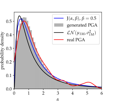
Figure 1: Comparison of a sectional view of the Jeffreys prior w.r.t. $\alpha$ (blue line) with some PGA distributions: approximated distribution of real accelerograms via Gaussian kernels in red, histogram of the generated signals in gray, and log-normal fit of the distribution in black.

In practice, due to the use of Markov Chain Monte Carlo (MCMC) methods (see section 5.2) to sample the a posteriori distribution, the prior must be evaluated (up to a multiplicative constant) many times in the calculations. Because of its computational complexity due to the integrals to be computed, we decided to perform evaluations of the prior on an experimental design based on a fine-mesh grid of $\Theta$ (here $[0,\infty)^{2}$) and to build an interpolated approximation of the Jeffreys prior from this design. This strategy is more suitable for our numerical applications and very tractable because the domain $\Theta$ is only two-dimensional. Figure 2 gives a plot of the Jeffreys prior. To be precise, $500\times 500$ prior values have been computed for $\alpha\in[10^{-5},10]$ and $\beta\in[10^{-3},2]$. A linear interpolation has been processed from these.

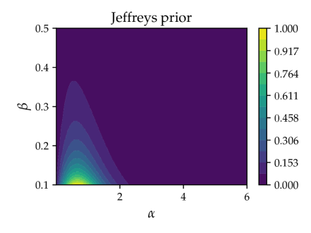
Figure 2: The Jeffreys prior calculated from PGA and plotted in the subdomain $[0,6]\times[0.1,0.5]$.

4.3 Discussion

The computational complexity of the Jeffreys prior is not in itself a major drawback. Depending solely on the distribution of the IM, its initial calculation will quickly be valued at the scale of an installation such as a nuclear plant which comprises several Structures and Components (SCs) whose fragility curves must be evaluated. Compared to methodologies that aim to define a prior on the basis of prior mechanical calculations which are specific to SCs by definition, the advantage of the Jeffreys prior is its generic character as will be seen in the applications section of this paper (section 6). Moreover, this prior is completely defined, it does not depend on an additional subjective choice.

The Jeffreys prior is known to be improper in numerous common cases (i.e. it cannot be normalized as a probability). In the present case, its asymptotic behavior is computed for different limits of $\theta=(\alpha,\beta)$ in A which shows that it is indeed improper. This characteristic is not an issue, as our work focuses on the posterior which is proper as proven in A. This property is essential as MCMC algorithms would not make any sense if the posterior were improper. These asymptotic expansions also provide complementary and essential insight into the Jeffreys prior. They make it possible to understand that its behavior in $\alpha$ is similar to that of a log-normal distribution having the same median as that of the IM (i.e. here 1.1 m/s²) with a variance which is the sum of the variance of the IM and of a term which depends on $\beta$. Figure 1 clearly illustrates this result.

5 Estimation tools, competing approaches and performance evaluation metrics

In this section, we first present the Bayesian estimation tools and the Monte-Carlo reference method to which we refer to evaluate the relevance of the log-normal model when the number of data allows it. Then, to evaluate the performance of the Jeffreys prior on practical cases, we present two competing approaches that we implement. On the one hand, we apply the MLE method widely used in literature, coupled with a bootstrap technique. On the other hand, we apply a Bayesian technique implemented with the prior introduced by Straub and Der Kiureghian [12]. For a fair comparison we propose to calibrate the latter according to the results of Figure 1 which evinces that in $\alpha$ the distribution is similar to the PGA distribution of the synthetic and real signals. It would indeed be easy to calibrate it in such a way so as to skew comparisons, by considering, for instance, a too large variance. Finally, performance evaluation metrics are defined.

5.1 Fragility curves estimations via Monte-Carlo

Here we assume that a validation data set $(\mathbf{a}^{\mathrm{MC}},$ $\mathbf{z}^{\mathrm{MC}})$ $=$ $((a_{i}^{\mathrm{MC}})_{i=1}^{N^{\mathrm{MC}}}$, $(z_{i}^{\mathrm{MC}})_{i=1}^{N^{\mathrm{MC}}})$ is available. This section describes how from such a large data set a fragility curve can be obtained by nonparametric estimation that can serve as a reference. This way, our estimations (based on a small data set and parametric estimation) can be compared with this reference.

Good candidates are Monte-Carlo (MC) estimators which estimate the expected number of failures locally w.r.t. the IM. We first need to define a subdivision of the IM values and to estimate the failure probability on each of the sub-intervals. Regular subdivisions are not appropriate because the observed IMs are not uniformly distributed. We follow the suggestion by Trevlopoulos et al. [22] to take clusters of the IM using K-means. Given such $N_{c}$ clusters $(K_{j})_{j=1}^{N_{c}}$, the Monte-Carlo fragility curve estimated at the centroids $(c_{j})_{j=1}^{N_{c}}$ is expressed as

$$P_{f}^{\mathrm{MC}}(c_{j})=\frac{1}{n_{j}}\sum_{i,\,a_{i}^{\mathrm{MC}}\in K_{j}}z_{i}^{\mathrm{MC}},$$ (19)

where $n_{j}$ is the sample size of cluster $K_{j}$. An asymptotic confidence interval for this estimator can also be derived using its Gaussian approximation. It is accepted that a MC-based fragility curve is a reference curve because it is not based on any assumption.

5.2 Fragility curves estimations in the Bayesian framework

To benefit from the Bayesian theory introduced in section 3 and the reference prior construction presented in section 4, the relevant method is to derive the posterior defined in equation (4) and to generate, according to that distribution, samples of $\theta$ conditioned on the observed data. Those a posteriori generations of $\theta$ can be performed thanks to MCMC methods. We have implemented an adaptive Metropolis-Hastings (M-H) algorithm with Gaussian transition kernel and covariance adaptation [52]. Such an algorithm allows sampling from a probability density known up to a multiplicative constant. In this context, the a posteriori samples of $\theta$ can be used to define credibility intervals for the log-normal estimates of the fragility curves.

5.3 Multiple MLE by bootstrapping

The best known parameter estimation method is the MLE, defined as the maximal argument of the likelihood derived from the observed data:

$$\hat{\theta}^{\mathrm{MLE}}_{k}=\operatorname*{arg\,max}_{\theta\in\Theta}\ell_{k}(\mathbf{z}|\mathbf{a},\theta).$$ (20)

A common method for obtaining a wide range of $\theta$ estimates is to compute multiple MLE by bootstrapping. Denoting the data set size by $k$, bootstrapping consists in doing $L$ independent draws with replacement of $k$ items within the data set. Those lead to $L$ different likelihoods from the $k$ initial observations, and so to $L$ values of the estimator which can be averaged. In the context of fragility curves, this method is widespread (e.g., [10, 11, 53, 54, 14]). The convergence of the MLE and the relevance of this method is stated in [55]. Nevertheless the bootstrap method is often limited by the irregularity of the results for small values of $k$ (e.g., [7]). In this context, the $L$ values of $\theta$ are used to define confidence intervals for the log-normal estimates of the fragility curves.

5.4 Example of a prior from literature for log-normal seismic fragility curves

For comparison purposes, we choose the prior suggested by Straub and Der Kiureghian – called the SK prior – which is defined as the product of a normal distribution for $\ln(\alpha)$ and the improper distribution $1/\beta$ for $\beta$, namely:

$$\pi_{SK}(\theta)\propto\frac{1}{\alpha\beta}\exp\Big{(}-\frac{(\log\alpha-\mu)^{2}}{2\sigma^{2}}\Big{)}.$$ (21)

In [12] the parameters $\mu$ and $\sigma$ of the log-normal distribution are chosen to generate a non-informative prior. As specified in the introduction to section 5, for a fair comparison with the approach proposed in this paper, we decided to choose $\mu$ and $\sigma$ being equal to the mean and the standard deviation of the logarithm of the IM. This choice is consistent with the fact that the Jeffreys prior is similar to a log-normal distribution with these parameters (see Figure 1). The prior $\pi_{SK}(\theta)$ is plotted in Figure 3.

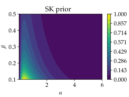
Figure 3: Prior suggested by Straub and Der Kiureghian [12] and plotted in the subdomain $[0,6]\times[0.1,0.5]$. It is expressed in equation (21) and scaled on a log-normal estimation of the PGA’s distribution.

An analysis of the posterior which results from the SK prior is given in A. It shows that the posterior is improper. This statement jeopardizes the validity of any a posteriori estimates using MCMC methods. This issue is nevertheless manageable with the consideration of a truncation w.r.t. $\beta$. In B we verify that the same issue still stands within the authors’ original framework which is slightly different from ours.

5.5 Performance evaluation metrics

To have a clear view of the performance of the proposed approach, we consider two quantitative metrics which can be calculated for each of the methods described in the previous subsections. We consider the sample $(\mathbf{a},\mathbf{z})$. We denote by $a\mapsto P_{f}^{|\mathbf{a},\mathbf{z}}(a)$ the random process defined as the fragility curve conditional to the sample (the probability distribution of $P_{f}^{|\mathbf{a},\mathbf{z}}(a)$ is inherited from the a posteriori distribution of $\theta$). For each value $a$ the $r$-quantile of the random variable $P_{f}^{|\mathbf{a},\mathbf{z}}(a)$ is denoted by $q_{r}^{|\mathbf{a},\mathbf{z}}(a)$. We define:

• The conditional quadratic error:

  $$\mathcal{E}^{Q|\mathbf{a},\mathbf{z}}=\mathbb{E}\big{[}\|P_{f}^{|\mathbf{a},\mathbf{z}}-P_{f}^{\mathrm{MLE}}\|_{L^{2}}^{2}|\mathbf{a},\mathbf{z}\big{]}=\int_{0}^{A_{\rm max}}\mathbb{E}\big{[}(P_{f}^{|\mathbf{a},\mathbf{z}}(a)-P_{f}^{\mathrm{MLE}}(a))^{2}|\mathbf{a},\mathbf{z}\big{]}da.$$ (22)

  $P_{f}^{\mathrm{MLE}}$ stands for the log-normal estimate of the fragility curve obtained by the MLE (see section 5.1) with the full data available according to the case study. We further check that this estimate is close to the reference curve obtained by MC when possible (see section 6).

• The conditional width of the $1-r$ credibility zone for the fragility curve:

  $$\mathcal{S}^{r|\mathbf{a},\mathbf{z}}=\|q_{1-{r/2}}^{|\mathbf{a},\mathbf{z}}-q_{{r/2}}^{|\mathbf{a},\mathbf{z}}\|_{L^{2}}^{2}=\int_{0}^{A_{\rm max}}(q_{1-{r/2}}^{|\mathbf{a},\mathbf{z}}(a)-q_{{r/2}}^{|\mathbf{a},\mathbf{z}}(a))^{2}da.$$ (23)

To estimate such variables, we simulate a set of $L$ fragility curves $(P_{f}^{\theta_{i}|\mathbf{a},\mathbf{z}})_{i=1}^{L}$ where $(\theta_{i})_{i=1}^{L}$ is a sample of the a posteriori distribution of the model parameters obtained by MCMC. The empirical quantiles $\hat{q}_{r}^{\theta_{i=1}^{L}|\mathbf{a},\mathbf{z}}(a)$ of $(P_{f}^{\theta_{i}|\mathbf{a},\mathbf{z}}(a))_{i=1}^{L}$ are approximations of the quantiles $q_{r}^{|\mathbf{a},\mathbf{z}}(a)$ of the random variable $P_{f}^{|\mathbf{a},\mathbf{z}}(a)$. We derive

• The approximated conditional quadratic error:

  $$\hat{\mathcal{E}}_{L}^{Q|\mathbf{a},\mathbf{z}}=\frac{1}{L}\sum_{i=1}^{L}\|P_{f}^{\theta_{i}|\mathbf{a},\mathbf{z}}-P_{f}^{\mathrm{MLE}}\|_{L^{2}}^{2}.$$ (24)

• The approximated conditional width of the $1-r$ credibility zone for the fragility curve:

  $$\hat{\mathcal{S}}_{L}^{r|\mathbf{a},\mathbf{z}}=\|\hat{q}_{1-{r/2}}^{\theta_{i=1}^{L}|\mathbf{a},\mathbf{z}}-\hat{q}_{{r/2}}^{\theta_{i=1}^{L}|\mathbf{a},\mathbf{z}}\|_{L^{2}}^{2}.$$ (25)

The $L^{2}$ norms are integrals over $a\in[0,A_{\rm max}]$ which are approximated numerically using Simpson’s interpolation on a regular subdivision $0=A_{0}<\dots<A_{p}=A_{\rm max}$. In the forthcoming examples we use $A_{0}=0$, $A_{\rm max}=12\,\mathrm{m/s^{2}}$, $p=200$.

For the MLE with bootstrapping, we can define a conditional quadratic error as in equation (24) and conditional width of the $1-r$ confidence interval as in equation (25) using a bootstrapped sample $(\theta_{i})_{i=1}^{L}$.

6 Numerical applications

In this section, three case studies are examined. Two of them benefit from a large number of available simulation data which have been computed for validation purposes. They serve the derivation of a reference fragility curve (in accordance with section 5.1’s suggestion), and allow to validate the log-normal model for those.

Indeed, the first is a nonlinear oscillator, for which $N_{s}=10^{5}$ nonlinear simulations have been implemented for validation purposes as described in section 6.1. The second case study, described in section 6.2, corresponds to a piping system which is a part of a secondary line of a French Pressurized Water Reactor. In this case, only $N_{s}=10^{4}$ simulations have been performed due to the high computational cost. For both of them, estimations are performed from different testing data sets extracted from the set of the available nonlinear dynamical simulation results. Thus, different subsamples of size $k$ are considered, chosen negligible in front of $N_{s}$.

Another case study is treated within a supplementary material of this work, to illustrate the application of the method to practical experiments.

6.1 Case study 1: a nonlinear oscillator

The first case study - depicted in Figure 4 - relates to a single degree of freedom elastoplastic oscillator which exhibits kinematic hardening. This mechanical system reflects the essential features of the nonlinear responses of some real structures under seismic excitation and has already been used in several studies [22, 28, 35]. For a unit mass $m$, its equation of motion is:

$$\ddot{y}(t)+2\zeta\omega_{\text{L}}\dot{y}(t)+f(t)=-s(t)\ ,$$ (26)

with $s(t)$ a seismic signal. $\dot{y}(t)$ and $\ddot{y}(t)$ are respectively the relative velocity and acceleration of the mass. $\zeta$ is the damping ratio and $\omega_{\text{L}}$ is the circular frequency. The EDP of interest is the maximum in absolute value of the displacement of the mass, i.e. $\max_{t\in[0,T]}|y(t)|$ where $T$ is the duration of the seismic excitation. The failure criterion $C$ is chosen to be the $90\%$-level quantile of the maximum displacement calculated with $10^{5}$ artificial signals, i.e. $C=8.0\;10^{-3}$ m. Figure 5 shows the comparison between the reference MC-based fragility curve $P_{f}^{\mathrm{MC}}$ (equation (19)) and its log-normal estimate $P_{f}^{\mathrm{MLE}}$, both estimated via the results of the $10^{5}$ simulations. The log-normal fragility curve is here a good approximation of the reference curve.

Figure 4: Elastoplastic oscillator with kinematic hardening, with parameters $f_{\text{L}}=5$ Hz and $\zeta=2\%$. The yield limit is $Y=5.10^{-3}$ m and the post-yield stiffness is $20\%$ of the elastic stiffness, i.e. $a=0.2$.

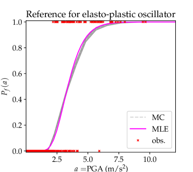
Figure 5: Reference fragility curve $P_{f}^{\mathrm{MC}}$ (see section 5.1) compared with $P_{f}^{\mathrm{MLE}}$ (see section 5.5) for the elastoplastic oscillator (case study 1). They are computed using the full data set generated ($10^{5}$ items). The red crosses represent the observations; 0 means no failure while 1 means failure.

The fragility curve estimates are shown in Figure 6. They result from $L=5000$ samples of $\theta$ generated with the implemented statistical methods (see section 5), which are based on two samples of nonlinear dynamical simulations of sizes $k=20$ and $k=30$. Although the intervals compared – that of the Bayesian framework and that of the MLE – are not of the same nature – credibility interval for the first versus confidence interval for the second – these results clearly illustrate the advantage of the Bayesian framework over the MLE for small samples. With the MLE appear irregularities characterized by null estimates of $\beta$, which result in “vertical” confidence intervals. In A, we prove indeed that the likelihood is easily maximized with $\beta=0$ when samples are partitioned into two disjoint subsets when classified according to IM values: the one for which there is no failure and the one for which there is failure. When few failures are observed in the initial sample, the bootstrap technique can moreover lead to the generation of a large number of such samples. This last statement is perceived better through the inspection of the raw values of $\theta$ generated in Figure 7. The degenerate $\beta$ values that result from the MLE appear clearly and no such phenomenon is observed in the Bayesian framework although it is also theoretically affected by this type of samples.

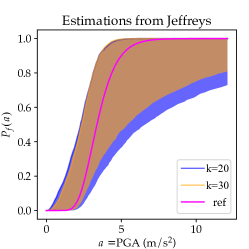
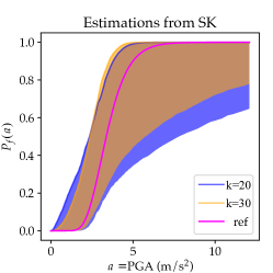
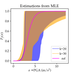
Figure 6: $95\%$ credibility (for Bayesian estimation) or confidence (for the MLE) intervals of fragility curves estimates, for the elastoplastic oscillator, resulting from a total of $L=5000$ estimations of $\theta$ using the statistical methods introduced in section 5.1: (from left to right) Bayesian estimation using the Jeffreys prior, Bayesian estimation using the SK prior, the MLE with bootstrapping. For each of them, two data samples of nonlinear dynamical simulations of two different sizes are considered ($k=20$ in blue, $k=30$ in orange). In magenta is plotted $P_{f}^{\mathrm{MLE}}$ (see section 5.5).

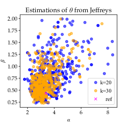
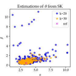
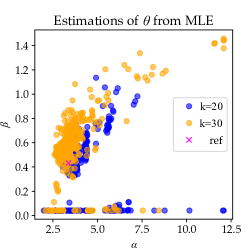
Figure 7: Scatter plots of the generated $\theta$ to estimate the fragility curves presented in Figure 6 for the elasto-plastic oscillator. For the three statistical methods and two data sets of nonlinear dynamical simulations (of size $k=20$ in blue and $k=30$ in orange) are plotted $500$ points from the $L=5000$ $\theta=(\alpha,\beta)$ estimated. The magenta crosses stand for $\theta^{\mathrm{MLE}}$ which is used for the computation of $P_{f}^{\mathrm{MLE}}$ (see section 5.5). This figure unveils both the irregularities characterized by null estimates of $\beta$ for the coupled MLE and bootstrap approach and the outliers generated from the SK prior.

Since the SK prior is calibrated to look like the Jeffreys prior, Figure 6 shows a strong similarity between the Bayesian estimates of the fragility curves obtained with these two priors. However, Figure 7 (middle) shows that many outliers are simulated with the SK prior. These values explain that the credibility intervals of the fragility curves are larger with the SK prior when $k=20$. This observation is supported theoretically by the calculation we provide in A. Indeed, we have shown a better convergence of the Jeffreys prior toward $0$ when $\beta\longrightarrow\infty$. This better asymptotic behavior obviously results in posteriors which happen to give a lower probability to outlier points – phenomena particularly noticeable when the data sample is small – as well as to the weight of the likelihood within the posterior.

For a better understanding of this phenomenon, we calculate the quantitative metrics defined in section 5.5. For any $k$ varying from $15$ to $100$, $m=200$ different draws of observations $(\mathbf{a}^{(j)},\mathbf{z}^{(j)})_{j=1}^{m}$ have been conducted to derive the metrics $\hat{\mathcal{E}}_{L,R}^{Q|\mathbf{a}^{(j)},\mathbf{z}^{(j)}}$, $\hat{\mathcal{S}}_{L,R}^{r|\mathbf{a}^{(j)},\mathbf{z}^{(j)}}$, $j\in\{1,\dots,m\}$, $R\in\{$‘MLE’, ‘SK’, ‘Jeffreys$\}$, $L=5000$, $1-r=95\%$. Their means and their $95\%$-confidence intervals are plotted in Figure 8. First, these plots demonstrate the interest of the Bayesian framework compared to the MLE approach, with small observation sets. Second, the performance of the Jeffreys posterior in comparison with the SK posterior is highlighted by the confidence interval endpoints of the quadratic error and the credibility interval. The latter highlights the effect of the better asymptotic behavior of the Jeffreys prior on the width of the credibility interval, which varies similarly while being smaller than that of the SK prior, thus highlighting its ability to generate fewer outliers for the pair $(\alpha,\beta)$ as expected.

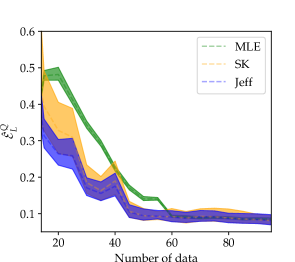
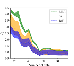
Figure 8: Performance evaluation metrics (see section 5.5) for the elasto-plastic oscillator computed by replications from independent draws in the full data set of nonlinear dynamical simulations and for sample sizes ranging from $k=15$ to $100$. Left: as a function of the number of observations, the dashed lines plot the quadratic errors and the shaded areas show their confidence intervals. Right: the dashed lines plot the widths of the credibility intervals (for the Bayesian estimation) or confidence intervals (for the MLE) and the shaded areas show their confidence intervals.

6.2 Case study 2 : piping system

This second case study concerns a piping system that is a part of a secondary line of a French Pressurized Water Reactor. This piping system was studied, experimentally and numerically, within the framework of the ASG program [56]. Figure 9 shows a view of the mock-up mounted on the shaking table Azalee of the EMSI laboratory of CEA/Saclay whereas the Finite Element Model (FEM) – based on beam elements – is shown in Figure 9-right. The latter has been implemented with the homemade FE code CAST3M [57] and has been validated via an experimental campaign.

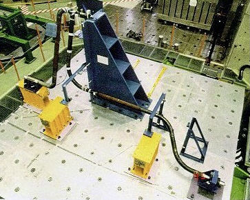
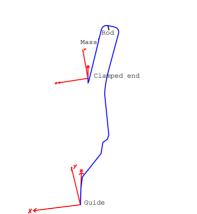
Figure 9: (left) Overview of the piping system on the Azalee shaking table and (right) Mock-up FEM.

The mock-up is a 114.3 mm outside diameter and 8.56 mm thickness pipe with a 0.47 elbow characteristic parameter, in carbon steel TU42C, filled with water without pressure. It has three elbows and a mass modeling a valve (120 kg) which corresponds to more than 30% of the total mass of the mock-up. One end of the mock-up is clamped whereas the other is supported by a guide in order to prevent the displacements in the X and Y directions. Additionally, a rod is placed on the top of the specimen to limit the mass displacements in the Z direction (see Figure 9-right). In the tests, the excitation is only imposed in the X direction. For this study, the artificial signals are filtered by a fictitious $2\%$ damped linear single-mode building at $5$ Hz, the first eigenfrequency of the $1\%$ damped piping system. As failure criterion, we consider excessive out-of-plane rotation of the elbow located near the clamped end of the mock-up, as recommended in [58]. The critical rotation considered is equal to $4.1^{\circ}$. This is the $90\%$-level quantile of a sample of nonlinear numerical simulations of size $10^{4}$.

Figure 10 shows the comparison between the reference MC-based fragility curve $P_{f}^{\mathrm{MC}}$ (equation (19)) and its log-normal estimate $P_{f}^{\mathrm{MLE}}$, both estimated via the results of $10^{4}$ simulations. The log-normal fragility curve is also here a good approximation of the reference curve.

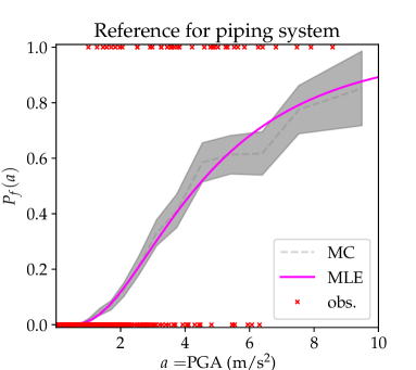
Figure 10: Reference fragility curve $P_{f}^{\mathrm{MC}}$ (see section 5.1) compared with $P_{f}^{\mathrm{MLE}}$ (see section 5.5) for the piping system (case study 2). They are computed using the full data set generated ($10^{4}$ items). The red crosses represent the observations; 0 means no failure while 1 means failure.

Similar estimations to those carried out for the elastoplastic oscillator have been performed for this case study and they highlight the same trends. Indeed, for sets of $L=5000$ values of $\theta$ – generated with each statistical method considered in this work – and for two sample sizes $k=20$ and $k=30$ of nonlinear dynamical simulations, Figure 11 shows as expected the superiority of the Bayesian framework over the coupled MLE and bootstrap approach. As in the case of the oscillator, we see the same irregularities with the MLE-based approach: the confidence intervals are ”quasi-vertical”, reflecting many estimates of $\beta$ equal to $0$. Moreover, the credibility intervals are wider with the SK prior than with the Jeffreys prior, reflecting here also more outliers of $\theta$ generated with the SK prior. These observations are clearly supported by the results presented in Figure 12.

For a more complete overview of their relative performance, the evaluation metrics described in section 5.5 have been computed in the same way as for the first case study: $m=200$ draws of data samples $(\mathbf{a}^{(j)},\mathbf{z}^{(j)})_{j=1}^{m}$ have been randomly chosen to compute, for any value of $k$ varying in a range from $15$ to $100$, $m$ values of the metrics $\hat{\mathcal{E}}_{L,R}^{Q|\mathbf{a}^{(j)},\mathbf{z}^{(j)}}$, $\hat{\mathcal{S}}_{L,R}^{r|\mathbf{a}^{(j)},\mathbf{z}^{(j)}}$, $R\in\{$‘MLE’, ‘SK’, ‘Jeffreys’$\}$, $L=5000$, $1-r=95\%$ . Their means and confidence intervals are proposed in Figure 13. These results confirm the better performance of the Jeffreys prior compared to the other two methods.

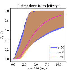
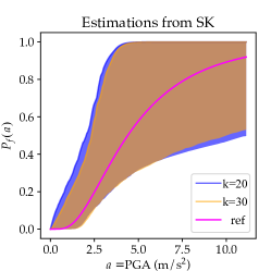
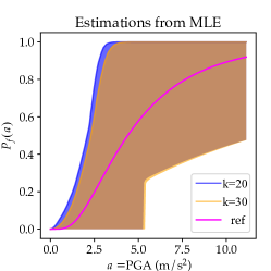
Figure 11: $95\%$ credibility (for Bayesian estimation) or confidence (for the MLE) intervals of fragility curves estimates, for the piping system, resulting from a total of $L=5000$ estimations of $\theta$ using the statistical methods introduced in section 5.1: (from left to right) Bayesian estimation using the Jeffreys prior, using the SK prior, the MLE with bootstrapping. For each of them, two data samples of nonlinear dynamical simulations of two different sizes are considered ($k=20$ in blue, $k=30$ in orange). In magenta is plotted $P_{f}^{\mathrm{MLE}}$ (see section 5.5).

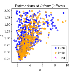
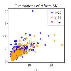
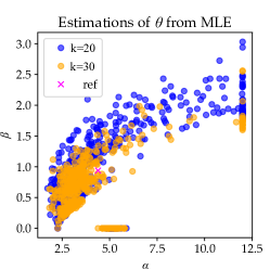
Figure 12: Scatter plots of the generated $\theta$ to estimate the fragility curves presented in Figure 11 for the piping system. For the three statistical methods and two data sets of nonlinear dynamical simulations (of size $k=20$ in blue and $k=30$ in orange) are plotted $500$ points from the $L=5000$ $\theta=(\alpha,\beta)$ generated. The magenta crosses plot $\theta^{\mathrm{MLE}}$ which is used for the computation of $P_{f}^{\mathrm{MLE}}$ (see section 5.5). This figure unveils both the irregularities characterized by null estimates of $\beta$ for the coupled MLE and bootstrap approach and the outliers generated from the SK prior.

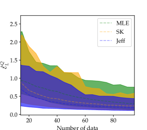
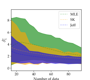
Figure 13: Performance evaluation metrics (see section 5.5) for the piping system computed by replications from independent draws in the full data set of nonlinear dynamical simulations and for sample sizes ranging from $k=15$ to $100$. Left: as a function of the number of observations, the dashed lines plot the quadratic errors and the shaded areas show their confidence intervals. Right: the dashed lines plot the widths of the credibility intervals (for the Bayesian estimation) or confidence intervals (for the MLE) and the shaded areas show their confidence intervals.

7 Conclusion

Assessing the seismic fragility of Structures and Components (SCs) when few data are available is a daunting task. The Bayesian framework is known to be efficient for these kinds of problems. Nevertheless, the choice of the prior remains tricky because it has a non-negligible influence on the a posteriori distribution and therefore on the estimation of any quantity of interest linked to the fragility curves.

So, based on the reference prior theory to define an objective prior, we have derived, for the first time in this field of study, the Jeffreys prior for the log-normal model with binary data that indicate the state of the structure (e.g., failure or non-failure). In doing so, this prior is completely defined; it does not depend on an additional subjective choice.

This work is also an opportunity to have a better theoretical understanding of the conditions that allow to have non-degenerate fragility curves (i.e., no curves in the form of unit step functions) in practice. This is indeed an inevitable issue when data are limited, since they are induced by the very composition of the data sample. Thus, although it affects all approaches, in comparison with the classical ones of the literature, we show rigorously – i.e., both theoretically and numerically – the robustness and advantages of the proposed approach in terms of regularization (absence of degenerate functions when sampling fragility curves with the a posteriori distribution) and stability (absence of outliers when sampling the a posteriori distribution of the parameters) for fragility curves estimation. The Jeffreys prior therefore leads to robust credibility intervals.

Although its numerical implementation is complex – i.e., more complex than a prior defined as the product of two classical distributions, such as log-normal distributions, for instance –, it is not a major obstacle. In fact, depending solely on the distribution of the IM, its initial calculation will be quickly valued on the scale of an industrial installation which includes several SCs whose fragility curves must be evaluated. For instance, in comparison to methodologies that aim to define, for a given SC, a prior based on mechanical calculations, the advantage of the Jeffreys prior is its generic nature. It can be applied to all SCs subject to the same seismic scenario, which largely compensates for the implementation of mechanical studies dedicated to each SC of interest. Additionally, the methodology can be implemented with any IM of interest, without additional complexity.

8 Acknowledgments

This research was supported by CEA (French Alternative Energies and Atomic Energy Commission) and SEISM Institute (www.institut-seism.fr/en/).

Appendix A Prior and posterior asymptotics

This appendix is dedicated to the asymptotic study of the density functions that are considered in this work. Those calculations provide a proof of the proper characteristics of the posterior distributions, needed to validate MCMC methods for sampling the posterior distributions. Also, the asymptotics of the Jeffreys prior can be compared to the ones of Straub and Der Kiureghian’s prior to state rigorously their different convergence rates. The derived asymptotics of the likelihood depend on the distribution of the observed data, inducing different phenomena which are discussed.

The analysis of the Jeffreys prior convergence rates requires an assumption about the IM’s distribution. Here we consider the following one.

Assumption 1.

The IM is distributed according to a log-normal distribution. i.e. there exist $\mu\in\mathbb{R}$ and $\sigma\in(0,+\infty)$ such that

$$p(a)=\frac{1}{\sqrt{2\pi\sigma^{2}}a}\exp\left({-\frac{(\log a-\mu)^{2}}{2\sigma^{2}}}\right).$$ (27)

This assumption, not far from reality, meets the discussion we conducted in section 5.4. It makes the SK prior being given by

$$\pi_{SK}(\theta)=\frac{1}{\sqrt{2\pi\sigma^{2}}\alpha\beta}\exp\left(-\frac{(\log\alpha-\mu)^{2}}{2\sigma^{2}}\right).$$ (28)

The appendix is organized as follows: we summarize our theoretical results about the asymptotic of the likelihood first (in A.1) and the prior density functions then (in A.2). A discussion and a comparison of the resulting posteriors’ proper characteristic are given in A.3. In A.4, potential scenarios issuing degenerate fragility curves are presented. The proofs are finally presented in A.5.

A.1 Likelihood asymptotic

The following proposition gives the asymptotic behaviors of the likelihood for different limits of $\theta=(\alpha,\beta)$.

Proposition 1.

Consider $k>1$ and a data sample $(\mathbf{a},\mathbf{z})=((a_{i})_{i=1}^{k},(z_{i})_{i=1}^{k})$. Introduce the vectors $\mathbf{N}=(z_{i}\mathbbm{1}_{a_{i}<\alpha}+(1-z_{i})\mathbbm{1}_{a_{i}>\alpha})_{i=1}^{k}$, $\log^{2}\frac{\mathbf{a}}{\alpha}=(\log^{2}\frac{a_{i}}{\alpha})_{i=1}^{k}$.

• Fix $\alpha>0$, then

  $$\ell_{k}(\mathbf{z}|\mathbf{a},\theta)\overset{\ }{\underset{\beta\rightarrow\infty}{\longrightarrow}}2^{-k}$$ (29)

  and

  $$\ell_{k}(\mathbf{z}|\mathbf{a},\theta)\underset{\beta\rightarrow 0}{=}O\left(\beta^{|\mathbf{N}|}e^{-\frac{\mathbf{N}^{T}\log^{2}\frac{\mathbf{a}}{\alpha}}{2\beta^{2}}}\right),$$ (30)

  where $|\mathbf{N}|=\sum_{i=1}^{k}N_{i}$.

• Fix $\beta>0$, then

  $$\ell_{k}(\mathbf{z}|\mathbf{a},\theta)\underset{\alpha\rightarrow 0}{=}O\left(|\log\alpha|^{|\mathbf{z}|-k}e^{-\frac{1}{2\beta^{2}}\sum_{i=1}^{k}(1-z_{i})(\log a_{i}-\log\alpha)^{2}}\right)$$ (31)

  and

  $$\ell_{k}(\mathbf{z}|\mathbf{a},\theta)\underset{\alpha\rightarrow\infty}{=}O\left(\log(\alpha)^{-|\mathbf{z}|}e^{-\frac{1}{2\beta^{2}}\sum_{i=1}^{k}z_{i}(\log a_{i}-\log\alpha)^{2}}\right),$$ (32)

  where $|\mathbf{z}|=\sum_{i=1}^{k}z_{i}$ is the number of failures in the observed sample.

Under general circumstances, the vector $\mathbf{N}$ is not null and the likelihood converges rapidly to zero when $\beta\longrightarrow 0$. Under some special circumstances, however, the vector $\mathbf{N}$ is null and the likelihood does not converge to zero when $\beta\longrightarrow 0$. This happens when the failure occurrences are perfectly separated, i.e. when there exists an open interval $U$ such that $\forall\alpha\in U,$ $\forall i,$ $z_{i}=1\iff a_{i}>\alpha$). Then the vector $\mathbf{N}$ is equal to ${\bf 0}$ for any $\alpha\in U$. This also happens when the observed sample only contains failures, resp. no-failures. Then the vector $\mathbf{N}$ is equal to ${\bf 0}$ for $\alpha<\min(a_{i})$, resp. $\alpha>\max(a_{i})$.

A.2 Prior asymptotic

The next three propositions give the asymptotics of the Jeffreys prior $J(\theta)$ for $\theta=(\alpha,\beta)$ in the four main directions of $(0,+\infty)^{2}$.

Proposition 2.

Fix $\alpha>0$, there exists $D^{\prime}(\alpha)>0$ such that

$$J(\theta)\underset{\beta\rightarrow 0}{\sim}\frac{D^{\prime}(\alpha)}{\beta}.$$ (33)

Proposition 3.

There exists a constant $E^{\prime}>0$ such that for any $\alpha>0$

$$J(\theta)\underset{\beta\rightarrow\infty}{\sim}\frac{E^{\prime}}{\alpha\beta^{3}}.$$ (34)

Proposition 4.

Fix $\beta>0$, there exists $G^{\prime\prime}(\beta)>0$ such that

$$J(\theta)\underset{|\log\alpha|\rightarrow\infty}{\sim}G^{\prime\prime}(\beta)\frac{|\log\alpha|}{\alpha}\exp\left(-\frac{(\log\alpha-\mu)^{2}}{2\beta^{2}+2\sigma^{2}}\right).$$ (35)

A.3 Discussion about posteriors

Proper characteristic discussion

Those results confirm that the Jeffreys and the SK priors are not proper with respect to $\beta$. For the Jeffreys prior, its divergence and convergence rates with respect to $\beta$ make its resulting posterior being proper when the prior is coupled with the likelihood –while the particular circumstances making the likelihood divergent when $\beta\rightarrow 0$ as raised in A.1 do not stand–. However, one can see that this is not the case for the SK posterior, which is not integrable w.r.t. $\beta$, because of its too low convergence rate at $+\infty$. This makes the MCMC estimates from this posterior impossible to validate, unless considering a truncation of the distribution. This statement explains the generation of a posteriori outliers using the SK prior. Note that Straub and Der Kiureghian consider this prior within a Bayesian framework in [12] which is slightly different from ours. In B we confirm that the posterior is not proper even when derived in the exact framework of [12].

Asymptotic comparison of the Jeffrey and the SK priors

By comparing the Jeffreys prior asymptotics with the SK prior asymptotics (28), we can note that:

• Regarding their asymptotics w.r.t. $\beta$, while their divergence rates are the same when $\beta\longrightarrow 0$, the Jeffreys prior performs better when $\beta\longrightarrow\infty$:

  $$J(\theta)\underset{\beta\rightarrow\infty}{\propto}\beta^{-2}\pi_{SK}(\theta).$$

  Consequently, the SK posterior gives higher probabilities to high values of $\beta$ compared to the Jeffreys prior.

• Regarding their asymptotics w.r.t. $\alpha$, both are asymptotically close to a log-normal distribution, with a disadvantage on the side of the Jeffreys prior, for which the asymptotic variance is derived by adding $\beta^{2}$ to the one of the SK prior. Thus, while for small values of $\beta$ (smaller than $\sigma$) both priors remain comparable w.r.t. $\alpha$, the Jeffreys prior gives higher probabilities to outliers $\alpha$ when $\beta$ is high itself. However, as seen above large values of $\beta$ have a quite low probability in the case of the Jeffreys prior compared with the SK prior. This explains why the generation of such outliers $\alpha$ has not been encountered in the estimates generated in our paper.

A.4 On the consequences of the non-convergence of the likelihood towards 0 when $\beta$ tends towards 0 in certain circumstances

Proposition 1 states different convergence rates according to the way the observed data are distributed. Indeed, as explained before, three kinds of samples will lead to a divergence of the likelihood when $\beta$ tends toward $0$: (i) a sample orderly by “no failure” and “failure” events when classified by IM values, (ii) a sample with only “no failure” events and (iii) a sample with only “failure” events. Such samples lead to unrealistic estimations of $\beta$ as $0$ within the MLE estimates which result in unit step fragility curves functions. In such circumstances, the likelihood is not fully controlled by the priors implemented in this work, leading to improper posteriors when integrated around $\beta\longrightarrow 0$. Those might issue degenerate fragility curves as well, yet the validity of such a posteriori estimates would remain questionable in that case.

A.5 Proofs

In this section, we prove propositions 1 to 4. We first state some upper bounds for the function $\gamma\mapsto[\Phi(\gamma)(1-\Phi(\gamma))]^{-1}$.

Lemma 1.

For any $\gamma\in\mathbb{R}$, $[\Phi(\gamma)(1-\Phi(\gamma))]^{-1}\leq 4\exp\left(2\gamma^{2}/\pi\right)$.

Lemma 2.

For any $\gamma\in\mathbb{R}$,

$$\Phi(\gamma)(1-\Phi(\gamma))\geq\frac{\sqrt{2/\pi}\exp(-\gamma^{2}/2)}{(|\gamma|+\sqrt{\gamma^{2}+4})}.$$ (36)

Proof of lemma 1.

From the folliwing inequality about the $\operatorname{erf}$ function [59]:

$$\forall\gamma>0,\,\sqrt{1-e^{-\frac{\gamma^{2}}{2}}}\leq\operatorname{erf}(\gamma/\sqrt{2})\leq\sqrt{1-e^{-2\frac{\gamma^{2}}{\pi}}},$$

we can deduce that, for any $\gamma>0$,

$$e^{-\frac{2\gamma^{2}}{\pi}}\leq 1-\operatorname{erf}(\gamma/\sqrt{2})^{2}\leq e^{-\frac{\gamma^{2}}{2}},$$

$$\frac{1}{4}e^{-\frac{2\gamma^{2}}{\pi}}\leq\frac{1}{4}\left(1-\operatorname{erf}\left({\gamma}/{\sqrt{2}}\right)\right)\left(1+\operatorname{erf}\left({\gamma}/{\sqrt{2}}\right)\right)\leq\frac{1}{4}e^{-\frac{\gamma^{2}}{2}},$$

the middle hand term being equal to $\Phi(\gamma)(1-\Phi(\gamma))$. This implies:

$$[\Phi(\gamma)(1-\Phi(\gamma))]^{-1}\leq 4e^{\frac{2\gamma^{2}}{\pi}},$$

hence the result for $\gamma>0$.

While it is clear that the inequality still stands for $\gamma=0$, notice from $\Phi(-\gamma)=1-\Phi(\gamma)\,\forall\gamma\in\mathbb{R}$ that $\gamma\mapsto\Phi(\gamma)(1-\Phi(\gamma))$ is an even function. Thus, the inequality still stands for any $\gamma<0$; this concludes the proof of the lemma. ∎

Proof of lemma 2.

Komatsu’s inequality [60, p. 17]:

$$\forall\gamma>0,\,\frac{2}{\sqrt{\gamma^{2}+4}+\gamma}\leq e^{\frac{\gamma^{2}}{2}}\int_{\gamma}^{\infty}e^{-\frac{t^{2}}{2}}dt\leq\frac{2}{\sqrt{\gamma^{2}+2}+\gamma}$$

implies

$$\forall\gamma>0,\,\frac{2e^{-\frac{\gamma^{2}}{2}}}{\sqrt{\gamma^{2}+4}+\gamma}\leq\sqrt{2\pi}(1-\Phi(\gamma))\leq\frac{2e^{-\frac{\gamma^{2}}{2}}}{\sqrt{\gamma^{2}+2}+\gamma}.$$

As $0<\Phi<1$ it comes for $\gamma>0$

$$\Phi(\gamma)(1-\Phi(\gamma)) \geq\frac{2e^{-\frac{\gamma^{2}}{2}}}{\sqrt{\gamma^{2}+4}+\gamma}\left(1-\frac{2e^{-\frac{\gamma^{2}}{2}}}{\sqrt{\gamma^{2}+2}+\gamma}\right)\geq\frac{\sqrt{2/\pi}e^{-\frac{\gamma^{2}}{2}}}{\sqrt{\gamma^{2}+4}+\gamma}.$$

Finally, as $\Phi(-\gamma)=1-\Phi(\gamma)$, $\gamma\mapsto\Phi(\gamma)(1-\Phi(\gamma))$ is an even function and we have for any $\gamma\in\mathbb{R}$

$$\Phi(\gamma)(1-\Phi(\gamma))\geq\frac{\sqrt{2/\pi}e^{-\frac{\gamma^{2}}{2}}}{\sqrt{\gamma^{2}+4}+|\gamma|}.$$

∎

A.5.1 Proof of Proposition 1

We recall the likelihood expression:

$$\ell_{k}(\mathbf{z}|\mathbf{a},\theta) =\prod_{i=1}^{k}\Phi\left(\frac{\log a_{i}-\log\alpha}{\beta}\right)^{z_{i}}\left(1-\Phi\left(\frac{\log a_{i}-\log\alpha}{\beta}\right)\right)^{1-z_{i}}$$

$$=\exp\left[\sum_{i=1}^{k}\left(z_{i}\log\Phi(\gamma_{i})+(1-z_{i})\log(1-\Phi(\gamma_{i}))\right)\right],$$

denoting $\gamma_{i}=\beta^{-1}\log\frac{a_{i}}{\alpha}$.

To treat the case $\beta\longrightarrow\infty$ we remark that while $\alpha$ is fixed, the quantities $\Phi(\gamma_{i})$ all converge to ${1}/{2}$. The product of those limits gives the limit $\ell_{k}(\mathbf{z}|\mathbf{a},\theta)\overset{\ }{\underset{\beta\rightarrow\infty}{\longrightarrow}}2^{-k}$.

For the other cases, we remind that $\Phi(x)=\frac{1}{2}(1+\operatorname{erf}(x/\sqrt{2}))$ and $\operatorname{erf}(x)\underset{x\rightarrow\infty}{=}1-\frac{e^{-x^{2}}}{x\sqrt{\pi}}+o\left(\frac{e^{-x^{2}}}{x}\right)$, leading to

$$\Phi(x)\underset{x\rightarrow\infty}{=}1-\frac{e^{-\frac{x^{2}}{2}}}{x\sqrt{2\pi}}+o\left(\frac{e^{-\frac{x^{2}}{2}}}{x}\right).$$ (37)

Consider an $i\in\{1,\dots,k\}$ and compute

$$z_{i}\log\Phi(\gamma_{i})+(1-z_{i})\log(1-\Phi(\gamma_{i}))$$

$$\underset{\gamma_{i}\rightarrow\infty}{=}z_{i}\log\left(1-\frac{e^{-\frac{\gamma_{i}^{2}}{2}}}{\gamma_{i}\sqrt{2\pi}}+o\left(\frac{e^{-\frac{\gamma_{i}^{2}}{2}}}{\gamma_{i}}\right)\right)+(1-z_{i})\log\left(\frac{e^{-\frac{\gamma_{i}^{2}}{2}}}{\gamma_{i}\sqrt{2\pi}}+o\left(\frac{e^{-\frac{\gamma_{i}^{2}}{2}}}{\gamma_{i}}\right)\right)$$

$$\underset{\gamma_{i}\rightarrow\infty}{=}-z_{i}\frac{e^{-\frac{\gamma_{i}^{2}}{2}}}{\gamma_{i}\sqrt{2\pi}}+(1-z_{i})\log\left(\frac{e^{-\frac{\gamma_{i}^{2}}{2}}}{\gamma_{i}\sqrt{2\pi}}\right)+o(1)$$

$$\underset{\gamma_{i}\rightarrow\infty}{=}-(1-z_{i})\frac{\gamma_{i}^{2}}{2}-(1-z_{i})\log(\gamma_{i}\sqrt{2\pi})+o(1).$$

Using the relation $\Phi(-x)=1-\Phi(x)$ leads to

$$z_{i}\log\Phi(\gamma_{i})+(1-z_{i})\log(1-\Phi(\gamma_{i}))\underset{\gamma_{i}\rightarrow-\infty}{=}-z_{i}\frac{\gamma_{i}^{2}}{2}-z_{i}\log(-\gamma_{i}\sqrt{2\pi})+o(1).$$

Going back to the likelihood asymptotics, we firstly fix $\alpha>0$ and suppose $\beta\longrightarrow 0$. Thus, denoting the vectors $\mathbf{N}=(z_{i}\mathbbm{1}_{a_{i}<\alpha}+(1-z_{i})\mathbbm{1}_{a_{i}>\alpha})_{i=1}^{k}$ and $\log^{2}\frac{\mathbf{a}}{\alpha}=(\log^{2}\frac{a_{i}}{\alpha})_{i=1}^{k}$, we obtain

$$\ell_{k}(\mathbf{z}|\mathbf{a},\theta)\underset{\beta\rightarrow 0}{=}\frac{C(\alpha)}{\sqrt{2\pi}^{|\mathbf{N}|}}\beta^{|\mathbf{N}|}e^{-\frac{\mathbf{N}^{T}\log^{2}\frac{\mathbf{a}}{\alpha}}{2\beta^{2}}+o(1)}\underset{\beta\rightarrow 0}{=}O\left(\beta^{|\mathbf{N}|}e^{-\frac{\mathbf{N}^{T}\log^{2}\frac{\mathbf{a}}{\alpha}}{2\beta^{2}}}\right),$$

where $|\mathbf{N}|=\sum_{i=1}^{k}N_{i}$ and $C(\alpha)=\prod_{i=1}^{k}\left|\log\frac{a_{i}}{\alpha}\right|^{N_{i}}$.

Secondly, fix $\beta>0$ to get

$$\ell_{k}(\mathbf{z}|\mathbf{a},\theta) \underset{\alpha\rightarrow\infty}{=}\frac{\beta^{|\mathbf{N}|}}{\sqrt{2\pi}^{|\mathbf{N}|}}\left(\prod_{i=1}^{k}\log\left(\frac{\alpha}{a_{i}}\right)^{-z_{i}}\right)e^{-\frac{1}{2\beta^{2}}\sum_{i=1}^{k}z_{i}(\log a_{i}-\log\alpha)^{2}+o(1)}$$

$$\underset{\alpha\rightarrow\infty}{=}O\left(\log(\alpha)^{-|\mathbf{z}|}e^{-\frac{1}{2\beta^{2}}\sum_{i=1}^{k}z_{i}(\log a_{i}-\log\alpha)^{2}}\right),$$

where $|\mathbf{z}|=\sum_{i=1}^{k}z_{i}$ is the number of failures in the observed sample. In the same way we have

$$\ell_{k}(\mathbf{z}|\mathbf{a},\theta)\underset{\alpha\rightarrow 0}{=} \frac{\beta^{|\mathbf{N}|}}{\sqrt{2\pi}^{|\mathbf{N}|}}\left(\prod_{i=1}^{k}\log\left(\frac{a_{i}}{\alpha}\right)^{-(1-z_{i})}\right)e^{-\frac{1}{2\beta^{2}}\sum_{i=1}^{k}(1-z_{i})(\log a_{i}-\log\alpha)^{2}+o(1)}$$

$$\underset{\alpha\rightarrow 0}{=} O\left(|\log\alpha|^{|\mathbf{z}|-k}e^{-\frac{1}{2\beta^{2}}\sum_{i=1}^{k}(1-z_{i})(\log a_{i}-\log\alpha)^{2}}\right).$$

A.5.2 Proof of proposition 2

Let $\alpha>0$. For $0\leq k\leq 2$, we consider $A_{k1,k2}=A_{k1}+A_{k2}$ with $A_{kj}$ defined in (17):

$$A_{k1,k2}=\int_{0}^{\infty}\log^{k}\frac{a}{\alpha}\frac{\Phi^{\prime}(\gamma(a))^{2}}{\Phi(\gamma(a))(1-\Phi(\gamma(a)))}p(a)da.$$

We have

$$A_{k1,k2} =\beta^{k+1}\int_{-\infty}^{\infty}F_{A_{k1,k2}}(\gamma)d\gamma,$$ (38)

$$F_{A_{k1,k2}}(\gamma) =\frac{\gamma^{k}}{2\sqrt{\pi^{3}\sigma^{2}}}\frac{e^{-\gamma^{2}}e^{-\frac{(\beta\gamma-\mu+\log\alpha)^{2}}{2\sigma^{2}}}}{\Phi(\gamma)(1-\Phi(\gamma))}.$$ (39)

By lemma 1 an upper bound can be derived for $F_{A_{k1k2}}$: for any $\gamma\in\mathbb{R},\,\beta>0$,

$$|F_{A_{k1,k2}}(\gamma)|\leq\tilde{C}|\gamma|^{k}e^{-\frac{1}{3}\gamma^{2}}$$ (40)

which defines an integrable function on $\mathbb{R}$, $\tilde{C}$ being a constant independent of $\gamma$ and $\beta$. Hence the limit

$$\lim_{\beta\rightarrow 0}\int_{-\infty}^{\infty}F_{A_{k1,k2}}(\gamma)d\gamma=\int_{-\infty}^{\infty}\frac{\gamma^{k}}{2\sqrt{\pi^{3}\sigma^{2}}}\frac{e^{-\gamma^{2}}e^{-\frac{(\mu-\log\alpha)^{2}}{2\sigma^{2}}}}{\Phi(\gamma)(1-\Phi(\gamma))}d\gamma.$$

The last integral is null when $k=1$ as the integrated function is odd in this case. Otherwise, it is the integral of positive-valued function a.e. and so it is a positive constant. This way, we can state $A_{k1,k2}\underset{\beta\rightarrow 0}{\sim}D_{k}(\alpha)\beta^{k+1}$ for some $D_{k}(\alpha)>0$ if $k=0,2$, and $A_{11,12}\underset{\beta\rightarrow 0}{=}o(\beta^{2})$.

Focusing back on the Fisher information matrix expression, it comes

$$\det\mathcal{I}(\theta)\underset{\beta\rightarrow 0}{=}\frac{D_{0}(\alpha)D_{2}(\alpha)}{\alpha^{4}\beta^{2}}+o\left(\frac{1}{\beta^{2}}\right).$$

Finally, we obtain:

$$J(\theta)\underset{\beta\rightarrow 0}{\sim}\frac{D^{\prime}(\alpha)}{\beta},$$ (41)

where $D^{\prime}(\alpha)>0$ is a constant independent of $\beta$.

A.5.3 Proof of proposition 3

We remind firstly the asymptotic expansion of the $\operatorname{erf}$ function in $0$:

$$\operatorname{erf}(\gamma)\underset{\gamma\rightarrow 0}{=}\frac{2}{\sqrt{\pi}}\gamma+O(\gamma^{2}),$$

which allows us to state the behavior of $\Phi(\gamma)$ when $\gamma\longrightarrow 0$:

$$\Phi(\gamma)\underset{\gamma\rightarrow 0}{=}\frac{1}{2}+\frac{1}{\sqrt{2\pi}}\gamma+O(\gamma^{2}).$$

We now fix $\alpha>0$ and consider $A_{k1,k2}=A_{k1}+A_{k2}$:

$$A_{k1,k2} =\int_{-\infty}^{\infty}\tilde{F}_{A_{k1,k2}}(x)dx,$$

$$\tilde{F}_{A_{k1,k2}}(x) =\frac{x^{k}}{2\sqrt{\pi^{3}\sigma^{2}}}\frac{e^{-\frac{x^{2}}{\beta^{2}}}e^{-\frac{(x-\mu+\log\alpha)^{2}}{2\sigma^{2}}}}{\Phi(\beta^{-1}x)(1-\Phi(\beta^{-1}x))}.$$

We note the convergence of $\tilde{F}_{A_{k1,k2}}(x)$ towards an integrable function when $\beta\longrightarrow\infty$. Moreover, lemma 1 allows us to bound $\tilde{F}_{A_{k1,k2}}$ as

$$|\tilde{F}_{A_{k1,k2}}(x)| \leq\frac{2|x|^{k}}{\sqrt{\pi^{3}\sigma^{2}}}e^{-\frac{(x-\mu+\log\alpha)^{2}}{2\sigma^{2}}}e^{2\frac{x^{2}}{\pi\beta^{2}}}\leq\frac{2|x|^{k}}{\sqrt{\pi^{3}\sigma^{2}}}e^{-\frac{(x^{2}-2(\mu-\log\alpha))^{2}}{4\sigma^{2}}}e^{\frac{(\mu+\log\alpha)^{2}}{2\sigma^{2}}},$$

for any $x\in\mathbb{R}$ and $\beta>2\sigma/\sqrt{\pi}$. This dominating function is integrable on $\mathbb{R}$. Thus, $A_{k1,k2}$ admits a limit when $\beta\longrightarrow\infty$ expressed by:

$$\lim_{\beta\rightarrow\infty}A_{k1,k2}=E_{k}(\alpha)=\int_{-\infty}^{\infty}\frac{2x^{k}}{\sqrt{\pi^{3}\sigma^{2}}}e^{-\frac{(x-\mu+\log\alpha)^{2}}{2\sigma^{2}}}dx=\frac{2\sqrt{2}}{\pi}\mathbb{E}[X^{k}],$$

with $X\sim\mathcal{N}(\mu-\log\alpha,\sigma^{2})$. We can now recall the expression of the Jeffreys prior:

$$J(\theta)^{2}=\left|\frac{1}{\alpha^{2}\beta^{6}}A_{01,02}A_{21,22}-\frac{1}{\alpha^{2}\beta^{6}}A_{11,12}^{2}\right|,$$

we deduce that it is equivalent to $(E_{0}(\alpha)E_{2}(\alpha)-E_{1}^{2}(\alpha))/\alpha^{2}\beta^{6}$ when $\beta\longrightarrow\infty$. Finally,

$$J(\theta)\underset{\beta\rightarrow\infty}{\sim}\frac{E^{\prime}}{\alpha\beta^{3}},$$

with $E^{\prime}=\sqrt{E_{0}(\alpha)E_{2}(\alpha)-E_{1}^{2}(\alpha)}=2\sigma/\pi$.

A.5.4 Proof of proposition 4

As a preliminary result, we use equation (37) to obtain

$$\Phi(\gamma)(1-\Phi(\gamma))\underset{|\gamma|\longrightarrow\infty}{\sim}\frac{e^{\frac{-\gamma^{2}}{2}}}{|\gamma|\sqrt{2\pi}}.$$ (42)

We consider $A_{k1,k2}=A_{k1}+A_{k2}$:

$$A_{k1,k2}=C^{\prime}\int_{0}^{\infty}\left(\log\frac{a}{\alpha}\right)^{k}\frac{e^{-\frac{1}{\beta^{2}}\log^{2}\frac{a}{\alpha}}e^{-\frac{(\log a-\mu)^{2}}{2\sigma^{2}}}}{\Phi(\beta^{-1}\log\frac{a}{\alpha})\left(1-\Phi(\beta^{-1}\log\frac{a}{\alpha})\right)}\frac{da}{a},$$

denoting $C^{\prime}=\sqrt{4\pi^{3}\sigma^{2}}^{-1}$. By substitution

$$\nu=\log a-\frac{\sigma^{2}}{\sigma^{2}+\beta^{2}}\log\alpha-\frac{\beta^{2}}{\sigma^{2}+\beta^{2}}\mu=\log a-r\log\alpha-s\mu,$$

we get

$$A_{k1,k2} =C^{\prime}\int_{-\infty}^{\infty}\hat{F}_{A_{k1,k1}}(\nu)d\nu,$$

$$\hat{F}_{A_{k1,k1}}(\nu) =(\nu+(r-1)\log\alpha+s\mu)^{k}\frac{e^{-\frac{(\nu+(r+1)\log\alpha+s\mu)^{2}}{\beta^{2}}}e^{-\frac{(\nu+r\log\alpha+(s-1)\mu)^{2}}{2\sigma^{2}}}}{\left[\Phi(1-\Phi)\right](h_{\beta}(\nu))},$$

where $h_{\beta}(\nu)=\beta^{-1}(\nu+(r-1)\log\alpha+s\mu)$. Using equation (42), we obtain

$$\left[\Phi(1-\Phi)\right](h_{\beta}(\nu))\underset{|\log\alpha|\rightarrow\infty}{\sim}\frac{\beta e^{-\frac{(\nu+(r-1)\log\alpha+s\mu)^{2}}{2\beta^{2}}}}{|\nu+(r-1)\log\alpha+s\mu|\sqrt{2\pi}}.$$ (43)

Then for a clear sight of the asymptotic behavior of $\hat{F}_{A_{k1,k2}}$ we compute

$$-\frac{(\nu+(r-1)\log\alpha+s\mu)^{2}}{2\beta^{2}}-\frac{(\nu+r\log\alpha+(s-1)\mu)^{2}}{2\sigma^{2}}$$

$$=-\left(\frac{1}{2\beta^{2}}+\frac{1}{2\sigma^{2}}\right)\nu^{2}-\left(\frac{((r-1)\log\alpha+s\mu)^{2}}{2\beta^{2}}+\frac{(r\log\alpha+(s-1)\mu)^{2}}{2\sigma^{2}}\right)$$

$$=-\left(\frac{1}{2\beta^{2}}+\frac{1}{2\sigma^{2}}\right)\nu^{2}-\frac{(\log\alpha-\mu)^{2}}{2(\beta^{2}+\sigma^{2})}.$$ (44)

We expand $\hat{F}_{k1,k2}(\nu)=\sum_{j=1}^{k}C_{k}^{j}(r-1)^{j}\log^{j}\alpha(\nu+s\mu)^{k-j}g(\nu)$ $=\sum_{j=0}^{k}\hat{F}_{k1,k2}^{(j)}(\nu)$, with $g(\nu)$ defined as

$$g(\nu)=\frac{e^{-\frac{(\nu+(r+1)\log\alpha+s\mu)^{2}}{\beta^{2}}}e^{-\frac{(\nu+r\log\alpha+(s-1)\mu)^{2}}{2\sigma^{2}}}}{\left[\Phi(1-\Phi)\right](\beta^{-1}(\nu+(r-1)\log\alpha+s\mu))}.$$

The combination of equations (43) and (44) gives that the $\hat{F}_{k1,k2}^{(j)}$’s satisfy

$$\hat{F}_{k1,k2}^{(j)}(\nu)e^{\frac{(\log\alpha-\mu)^{2}}{2\beta^{2}+2\sigma^{2}}}(\log\alpha)^{-j}|\log\alpha|^{-1}\\ \overset{\ }{\underset{|\log\alpha|\rightarrow\infty}{\longrightarrow}}(\sqrt{2\pi}\beta)^{-1}C_{k}^{j}(r-1)^{j+1}(\nu+s\mu)^{k-j}e^{-\left(\frac{1}{2\beta^{2}}+\frac{1}{2\sigma^{2}}\right)\nu^{2}}.$$

Using lemma 2 allows to additionally dominate the above function by an integrable function as

$$|\hat{F}_{k1,k2}^{(j)}(\nu)|e^{\frac{(\log\alpha-\mu)^{2}}{2\beta^{2}+2\sigma^{2}}}|\log\alpha|^{-j-1}\leq\frac{\sqrt{2/\pi}e^{-\left(\frac{1}{2\beta^{2}}+\frac{1}{2\sigma^{2}}\right)\nu^{2}}}{|h_{\beta}(\nu)|+\sqrt{h_{\beta}(\nu)^{2}+4}}\leq\frac{1}{\sqrt{2\pi}}e^{-\left(\frac{1}{2\beta^{2}}+\frac{1}{2\sigma^{2}}\right)\nu^{2}}.$$

Therefore, we can switch the limits and the integration, and the following results stand:

$$C^{\prime\prime}\beta A_{01,02}e^{\frac{(\log\alpha-\mu)^{2}}{2\beta^{2}+2\sigma^{2}}}\underset{\log\alpha\rightarrow\infty}{=} (1-r)G\log\alpha-s\mu G+o(1),$$

$$C^{\prime\prime}\beta A_{11,12}e^{\frac{(\log\alpha-\mu)^{2}}{2\beta^{2}+2\sigma^{2}}}\underset{\log\alpha\rightarrow\infty}{=}-(1-r)^{2}G\log^{2}\alpha-s^{2}\mu^{2}G+2(1-r)s\mu G\log\alpha-G^{\prime}+o(1),$$

$$C^{\prime\prime}\beta A_{22,22}e^{\frac{(\log\alpha-\mu)^{2}}{2\beta^{2}+2\sigma^{2}}}\\ \underset{\log\alpha\rightarrow\infty}{=}(1-r)^{3}G\log^{3}\alpha-s^{3}\mu^{3}G-3(1-r)^{2}s\mu G\log^{2}\alpha\\ +3(1-r)s^{2}\mu^{2}G\log\alpha+3(1-r)G^{\prime}\log\alpha+o(1),$$

with $C^{\prime\prime}=(C^{\prime}\sqrt{2\pi})^{-1}$, $G=\sigma\beta\sqrt{2\pi(\beta^{2}+\sigma^{2})^{-1}}$ and $G^{\prime}=G^{2}/2\pi$. This way

$$C^{\prime\prime}\alpha\beta^{8}J(\theta)^{2}e^{\frac{(\log\alpha-\mu)^{2}}{2\beta^{2}+2\sigma^{2}}}\\ \underset{\log\alpha\rightarrow\infty}{=}3(r-1)^{2}s^{2}\mu^{2}G^{2}\log^{2}\alpha+3(r-1)^{2}s^{2}\mu^{2}G^{2}\log^{2}\alpha\\ +3(r-1)^{2}GG^{\prime}\log^{2}\alpha-4(r-1)^{2}s^{2}\mu^{2}G^{2}\log^{2}\alpha\\ -2(r-1)^{2}s^{2}\mu^{2}G^{2}\log^{2}\alpha-2(r-1)^{2}GG^{\prime}\log^{2}\alpha+o(\log^{2}\alpha).$$

Notice the above equality is still valid when $\log\alpha\longrightarrow-\infty$. Finally

$$J(\theta)\underset{|\log\alpha|\rightarrow\infty}{\sim}G^{\prime\prime}(\beta)\frac{|\log\alpha|}{\alpha}\exp\left(-\frac{(\log\alpha-\mu)^{2}}{2\beta^{2}+2\sigma^{2}}\right),$$

with

$$G^{\prime\prime}(\beta) =C^{\prime\prime-1}(r-1)^{2}GG^{\prime}\beta^{-4}=\frac{2\sigma^{3}\beta^{3}}{\sqrt{\pi}(\sigma^{2}+\beta^{2})^{7/2}}.$$

Appendix B A review of the properties of the SK posterior

In this paper we have compared our approach with the one that results from an adaptation of the prior suggested by Straub and Der Kiureghian [12]. We proved in A that this prior gives an improper posterior in our framework. This questions the validity of the MCMC estimates, which could explain the lower performance of the SK prior compared to the Jeffreys prior. The authors in [12] use the Bayesian methodology as we do, yet the consideration of uncertainties over the observed earthquake intensity measures and the equipment capacities lead to a slightly different likelihood. To stay convinced that the drawbacks of their prior that we highlighted are not due to our statistical choices, we dedicate this section to the study of the asymptotics of the posterior in the exact framework of [12].

First we present the exact model of Straub and Der Kiureghian for the estimation of seismic fragility curves in B.1, using notations consistent with our work. Second, the likelihood and its asymptotics are derived in B.2. Finally the convergence rates of the posterior are expressed in B.3 and allow us to conclude that the SK posterior is indeed improper.

B.1 Statistical model and likelihood

We consider the observations of earthquakes labeled $l=1,\dots,L$ at equipment labeled $i=1,\dots,I_{j}$ located in substations labeled $j=1,\dots,J$. The observed items are $(\mathbf{z}_{jl},\hat{a}_{jl})_{j,l}$, $\mathbf{z}_{jl}=(z_{ijl})_{i}$ being the failure occurrences of the $I_{j}$ equipments at substation $j$ during earthquake $l$ ($z_{ijl}\in\{0,1\}$) and $\hat{a}_{jl}$ being the observed IM at substation $j$ during earthquake $l$ ($\hat{a}_{jl}\in(0,+\infty)$). They are assumed to follow the latent model presented below.

At substation $j$ the $l$-th earthquake results in an IM value $a_{jl}$ that is observed with an uncertainty multiplicative noise: $\log\hat{a}_{jl}=\log a_{jl}+\varepsilon_{jl}$ where $\varepsilon_{jl}\sim\mathcal{N}(0,\sigma_{\varepsilon}^{2})$. The noise variance $\sigma_{\varepsilon}^{2}$ is supposed to be known. The uncertain intrinsic capacity of equipment $i$ at substation $j$ is $r_{ij}\sim\mathcal{N}(\mu_{r},\sigma^{2}_{r})$ and $y_{jl}\sim\mathcal{N}(0,\sigma^{2}_{y})$ is the uncertain factor common to all equipment capacities at substation $j$ during earthquake $l$. The random variables $r_{ij}$, $y_{jl}$ and $\varepsilon_{jl}$ are supposed to be independent.

A failure for equipment $i$ at substation $j$ during earthquake $l$ is considered when the performance of the structural component $g_{ijl}$ satisfies $g_{ijl}>0$.This performance can be expressed as

$$g_{ijl}=\log\hat{a}_{jl}+\varepsilon_{jl}-y_{jl}-r_{ij}=x_{jl}-r_{ij}\ \mbox{ with }x_{jl}=\log\hat{a}_{jl}+\varepsilon_{jl}-y_{jl}.$$

This states the following conditional relation between the observed data:

$$p(z_{ijl}|\hat{a}_{jl},\Sigma)=\int_{\mathbb{R}}p(z_{ijl}|x_{jl},\hat{a}_{jl},\Sigma)\frac{\exp\left({-\frac{(x_{jl}-\log\hat{a}_{jl})^{2}}{2(\sigma^{2}_{\varepsilon}+\sigma^{2}_{y})}}\right)}{\sqrt{2\pi(\sigma_{\varepsilon}^{2}+\sigma_{y}^{2})}}dx_{jl},$$ (45)

denoting $\Sigma=(\sigma_{r},\,\sigma_{y},\,\mu_{r})$, and with

$$p(z_{ijl}|x_{jl},\hat{a}_{jl},\Sigma)=\Phi\left(\frac{x_{jl}-\mu_{r}}{\sigma_{r}}\right)^{z_{ijl}}\left(1-\Phi\left(\frac{x_{jl}-\mu_{r}}{\sigma_{r}}\right)\right)^{1-z_{ijl}},$$ (46)

when substation $j$ is affected only by one earthquake. Indeed, the method proposed in [12] considers the cases in which a substation may be affected by two successive earthquakes and takes into account the fact that its response to the second is correlated to its response to the first one. That would lead to a different likelihood. However, it is mentioned that this possibility concerns only a few data items. We, therefore, limit our calculations to the simplest case and we assume $l=L=1$, we thus drop the subscript $l$ in what follows.

Finally, the likelihood for this model can be expressed as:

$$\ell_{J}(\mathbf{z}|\mathbf{\hat{a}},\Sigma)=\prod_{j=1}^{J}\int_{\mathbb{R}}\prod_{i=1}^{I_{j}}p(z_{ij}|x_{j},\log\hat{a}_{j},\Sigma)\frac{\exp\left({-\frac{(x_{j}-\log\hat{a}_{j})^{2}}{2(\sigma^{2}_{\varepsilon}+\sigma^{2}_{y})}}\right)}{\sqrt{2\pi(\sigma_{\varepsilon}^{2}+\sigma_{y}^{2})}}dx_{j},$$ (47)

denoting $\mathbf{z}=(\mathbf{z}_{j})_{j=1}^{J}$, $\mathbf{\hat{a}}=(\hat{a}_{j})_{j=1}^{J}$, and with the integrated conditional distribution being defined in equation (46).

In the Bayesian framework introduced in [12] the model parameter is $\Sigma$. We denote $\alpha=\exp\mu_{r}$, $\beta=\sqrt{\sigma_{r}^{2}+\sigma^{2}_{y}}$ and $\rho=\sigma^{2}_{y}/\beta^{2}$. Therefore, denoting $\theta=(\alpha,\beta,\rho)$, the knowledge of $\Sigma$ becomes equivalent to the one of $\theta$ and the likelihood of equation (47) can be expressed conditionally to $\theta$ instead of $\Sigma$:

$$\ell_{J}(\mathbf{z}|\mathbf{\hat{a}},\theta)=\prod_{j=1}^{J}\int_{\mathbb{R}}\prod_{i=1}^{I_{j}}\Psi^{z_{ij}}\left(\frac{x-\log\alpha}{\beta\sqrt{1-\rho}}\right)\frac{\exp\left({-\frac{(x-\log\hat{a}_{j})^{2}}{2(\sigma^{2}_{\varepsilon}+\rho\beta^{2})}}\right)}{\sqrt{2\pi(\sigma_{\varepsilon}^{2}+\rho\beta^{2})}}dx,$$ (48)

where the notation $\Psi^{z_{ij}}(\gamma)$ is used to denote $\Phi(\gamma)^{z_{ij}}(1-\Phi(\gamma))^{1-z_{ij}}$.

Straub and Der Kiureghian propose the following improper prior distribution for the parameter $\theta$:

$$\pi_{SK}(\theta)\propto\frac{1}{\beta\alpha}\exp\left(-\frac{(\log\alpha-\mu)^{2}}{2\sigma^{2}}\right)\mathbbm{1}_{0\leq\rho\leq 1}.$$ (49)

A posteriori estimations of $\theta$ are consequently generated from MCMC methods

$$p(\theta|\mathbf{z},\mathbf{\hat{a}})\propto\ell_{J}(\mathbf{z}|\mathbf{\hat{a}},\theta)\pi_{SK}(\theta).$$ (50)

B.2 Likelihood asymptotics

In this appendix we study the asymptotics of the likelihood defined in (48) when $\beta\longrightarrow\infty$. First we consider the substitution $u=(x-\log\hat{a}_{j})/\sqrt{\sigma_{\varepsilon}^{2}+\rho\beta^{2}}$ to express the likelihood as

$$\ell_{J}(\mathbf{z}|\mathbf{\hat{a}},\theta) =\prod_{j=1}^{J}\int_{\mathbb{R}}f_{j}^{\beta}(u)du,$$

$$f_{j}^{\beta}(u) =\prod_{i=1}^{I_{j}}\Phi(h_{j}^{\beta}(u))^{z_{ij}}(1-\Phi(h_{j}^{\beta}(u)))^{1-z_{ij}}\frac{e^{-\frac{u^{2}}{2}}}{\sqrt{2\pi}},$$

with

$$h_{j}^{\beta}(u)=\frac{(u+\log\hat{a}_{j})\sqrt{\sigma_{\varepsilon}^{2}+\rho\beta^{2}}-\log\alpha}{\beta\sqrt{1-\rho}}.$$

This way, reminding $0\leq\Phi(1-\Phi)\leq 1$, $f_{j}^{\beta}$ can be dominated for any $\beta,u$ by $u\mapsto e^{-u^{2}/2}/\sqrt{2\pi}$ and it converges as $\beta\longrightarrow+\infty$ as follows:

$$\lim_{\beta\rightarrow\infty}f_{j}^{\beta}(u)=\prod_{i=1}^{I_{J}}\Psi^{z_{ij}}\left(\frac{(u+\log\hat{a}_{j})\sqrt{\rho}}{\sqrt{1-\rho}}\right)\frac{e^{-\frac{u^{2}}{2}}}{\sqrt{2\pi}}.$$

This gives the following limit for the likelihood:

$$\lim_{\beta\rightarrow\infty}\ell_{J}(\mathbf{z}|\mathbf{\hat{a}},\theta)=\prod_{j=1}^{J}\int_{\mathbb{R}}\prod_{i=1}^{I_{j}}\Psi^{z_{ij}}\left(\frac{(u+\log\hat{a}_{j})\sqrt{\rho}}{\sqrt{1-\rho}}\right)\frac{e^{-\frac{u^{2}}{2}}}{\sqrt{2\pi}}du,$$ (51)

which is a positive quantity.

B.3 Posterior asymptotics

By combining equations (51), (50) and (49) we find the posterior asymptotics

$$p(\theta|\mathbf{z},\mathbf{\hat{a}})\underset{\beta\rightarrow{\infty}}{\sim}\frac{C}{\beta},$$ (52)

with $C$ being a positive constant. This makes the posterior improper w.r.t. $\beta$, with the same convergence rate as the one that was derived in our framework.

References

- Kennedy et al. [1980] R. P. Kennedy, C. A. Cornell, R. D. Campbell, S. J. Kaplan, F. Harold, Probabilistic seismic safety study of an existing nuclear power plant, Nuclear Engineering and Design 59 (1980) 315–338. doi:10.1016/0029-5493(80)90203-4.
- Kennedy and Ravindra [1984] R. P. Kennedy, M. K. Ravindra, Seismic fragilities for nuclear power plant risk studies, Nuclear Engineering and Design 79 (1984) 47–68. doi:10.1016/0029-5493(84)90188-2.
- Park et al. [1998] Y.-J. Park, C. H. Hofmayer, N. C. Chokshi, Survey of seismic fragilities used in PRA studies of nuclear power plants, Reliability Engineering & System Safety 62 (1998) 185–195. doi:10.1016/S0951-8320(98)00019-2.
- Kennedy [1999] R. P. Kennedy, Risk based seismic design criteria, Nuclear Engineering and Design 192 (1999) 117–135. doi:10.1016/S0029-5493(99)00102-8.
- Cornell [2004] C. A. Cornell, Hazard, ground motions and probabilistic assessments for PBSD, in: Proceedings of the International Workshop on Performance-Based Seismic Design - Concepts and Implementation, PEER Center, University of California, Berkeley, 2004, pp. 39–52.
- Grigoriu and Radu [2021] M. D. Grigoriu, A. Radu, Are seismic fragility curves fragile?, Probabilistic Engineering Mechanics 63 (2021) 103115. doi:10.1016/j.probengmech.2020.103115.
- Zentner et al. [2017] I. Zentner, M. Gündel, N. Bonfils, Fragility analysis methods: Review of existing approaches and application, Nuclear Engineering and Design 323 (2017) 245–258. doi:10.1016/j.nucengdes.2016.12.021.
- Gardoni et al. [2002] P. Gardoni, A. Der Kiureghian, K. M. Mosalam, Probabilistic capacity models and fragility estimates for reinforced concrete columns based on experimental observations, Journal of Engineering Mechanics 128 (2002) 1024–1038. doi:10.1061/(ASCE)0733-9399(2002)128:10(1024).
- Choe et al. [2007] D.-E. Choe, P. Gardoni, D. Rosowsky, Closed-form fragility estimates, parameter sensitivity, and bayesian updating for rc columns, Journal of Engineering Mechanics 133 (2007) 833–843. doi:10.1061/(ASCE)0733-9399(2007)133:7(833).
- Shinozuka et al. [2000] M. Shinozuka, M. Q. Feng, J. Lee, T. Naganuma, Statistical analysis of fragility curves, Journal of Engineering Mechanics 126 (2000) 1224–1231. doi:10.1061/(ASCE)0733-9399(2000)126:12(1224).
- Lallemant et al. [2015] D. Lallemant, A. Kiremidjian, H. Burton, Statistical procedures for developing earthquake damage fragility curves, Earthquake Engineering & Structural Dynamics 44 (2015) 1373–1389. doi:10.1002/eqe.2522.