Asteroids seen by JWST-MIRI: Radiometric Size, Distance and Orbit Constraints

Infrared measurements of asteroids are crucial for the determination of physical and thermal properties of individual objects, and for the understanding of the small-body populations in the solar system as a whole. But standard radiometric methods can only be applied if the orbit of an object is known, hence its position at the time of the observation. With JWST-MIRI observations the situation will change and many unknown, often very small, solar system objects will be detected. Later orbit determinations are difficult due to the faintness of the objects and the lack of dedicated follow-up concepts. We present MIRI observations of the outer-belt asteroid (10920) 1998 BC1 and an unknown object, detected in all 9 MIRI bands in close apparent proximity to (10920). We developed a new method ”STM-ORBIT” to interpret the multi-band measurements without knowing the object’s true location. The power of the new technique is that it determines the most-likely helio- and observer-centric distance and phase angle ranges, allowing to do a radiometric size estimate. The application to the MIRI fluxes of (10920) was used to validate the method. It leads to a confirmation of known radiometric size-albedo solution and puts constraints on the asteroid’s location and orbit in agreement with its true orbit. To back up the validation of the method, we obtained additional groundbased lightcurve observations of (10920), combined with Gaia data, which indicate a very elongated object (a/b $\geq$ 1.5), with a spin-pole at ($\lambda$, $\beta$)_ecl = (178^∘, +81^∘), with an estimated error of about 20^∘, and a rotation period of 4.861191 $\pm$ 0.000015 h. A thermophysical study of all available JWST-MIRI and WISE measurements leads to a size of 14.5 - 16.5 km (diameter of an equal-volume sphere), a geometric albedo p_V between 0.05 and 0.10, and a thermal inertia in the range 9 to 35 (best value 15) J m^-2s^-0.5K^-1. For the newly discovered MIRI object, the STM-ORBIT method revealed a size of 100-230 m. The new asteroid must be on a low-inclination orbit (0.7^∘ $<$ i $<$ 2.0^∘) and it was located in the inner main-belt region during JWST observations. A beaming parameter $\eta$ larger than 1.0 would push the size even below 100 meter, a main-belt regime which escaped IR detections so far. These kind of MIRI observations can therefore contribute to formation and evolution studies via classical size-frequency studies which are currently limited to objects larger than about one kilometer in size. We estimate that MIRI frames with pointings close to the ecliptic and only short integration times of a few seconds will always include a few asteroids, most of them will be unknown objects.

1 Introduction

The radiometric method is widely used to determine physical and thermal properties of small atmosphereless objects in the Solar System (e.g. Delbo et al., 2015). Measurements in the thermal infrared (IR) are combined with reflected light properties (usually represented by an object’s H, G1, G2 values) to find size-albedo solutions which explain the visual magnitudes and the IR fluxes simultaneously. If sufficient good-quality IR measurements are available, it is also possible to determine surface properties, like the roughness, the thermal inertia or thermal conductivity. A detailed modelling of the temperature distribution on the surface even allows to put constraints on spin or shape properties (e.g. Müller et al., 2017). Different thermal models are available, like the Standard Thermal Model (STM; Lebofsky et al. (1986)), the Near-Earth Thermal Model (NEATM, Harris (1998)), or more complex Thermophysical Models (TPM; Lagerros (1996, 1997, 1998); Rozitis & Green (2011)). The STM or NEATM are typically applied to survey data (e.g. Tedesco et al., 2002b, a; Usui et al., 2011; Mainzer et al., 2011), while TPM techniques are used in cases where spin-shape properties are known or for the interpretation of more complex data sets. But all these techniques have in common that they work for objects with known orbits where the helio-centric distance, the observer-centric distance and the phase angle are known for each individual observing epoch. In this context, the JWST asteroid observations and potential science cases are presented and discussed by Norwood et al. (2016), Rivkin et al. (2016) or Thomas et al. (2016), but the scientific aspects of IR detections of unknown object are not well covered yet.

Here, we present JWST-MIRI size and orbit constraints of the outer MBA (10920) 1998 BC1 and a faint, unknown object (Section 2). For (10920) we complement the MIRI observations by lightcurve and Gaia DR3 for spin-shape modeling, ATLAS survey data for an estimation of its H-magnitude, and WISE observations for a radiometric study. The derived MIRI photometric and astrometric information is given in Section 3, followed by a detailed radiometric thermophysical model (TPM) study for (10920) (Section 4). In Section 5 we exploit the possibilities and limitations of newly developed STM-ORBIT method for the determination of the object’s physical and orbital properties just based on IR data alone. We apply the new method first to the known asteroid (10920) for testing purposes and then to a newly discovered object where no orbit solution is available. The results are discussed in Section 6 and summarized in Section 7.

2 Observations

2.1 JWST-MIRI observations

A MIRI imaging mode (Bouchet et al., 2015) multi-filter measurement sequence was executed on July 14, 2022 as part of the JWST calibration program ”MIRI Imaging Filter Characterization”. The main-belt asteroid (10920) 1998 BC1 was the prime object, however, the individual images also show a faint object which moved with respect to (10920) and the background sources (see Fig. 1). This faint unknown object was in the 56.3^′′ $\times$ 56.3^′′ field-of-view (BRIGHTSKY sub-array with 512 $\times$ 512 pixels) in all 9 MIRI bands, while the much brighter MBA (10920) was found to be located at the edge or even outside the FOV in the long-wavelength measurements. In each of the nine MIRI filters, a set of 4 dithered images were taken, each with a frame time of 0.865 s (FASTR1 readout mode), and an exposure time of 21.632 s (F0560 band) or 8.653 s (for all other bands). The JWST data processing is done in three different stages, using the following pipeline modules for the MIRI imaging observations: calwebb_detector1 (L1): to process raw ramps data into uncalibrated slopes data (data quality initialization, saturation check, reference pixel correction, jump detection, slope fitting, reset anomaly correction, first/last frame correction, linearity & RSCD correction, dark subtractions); calwebb_image2 (L2): to process data from uncalibrated slope images into calibrated slope images (WCS information, background subtraction, flat-field correction, flux calibration, drizzle algorith to produce rectified 2-D products); calwebb_image3 (L3): to process the imaging data from calibrated slope images to mosaics and source catalogs (refine relative WCS, moving target WCS, background matching ”Skymatch”, outlier detection, image combination, source catalog, update of exposure level products).

For the dedicated (10920) observations presented here, we used the calibrated L2 images (corrected for detector and physical effects, and flux calibrated) where we found 4 individual (dithered) images per filter (for the astrometry and flux extraction). We also worked with the pipeline-processed calibrated L3 images (see Fig. 1 top row) with the 4 dithered images combined with respect to the moving target (10920) position, and manually combined L2 images after stacking onto the new object’s position (see Fig. 1 bottom row). For more details on the MIRI imaging mode, see the JWST-specific documentation. Table 1 summarizes details for the 36 individual data frames.

Table 1: MIRI imaging mode observations of asteroid (10920) 1998 BC1 were taken as part of a filter characterization calibration program^a.

No.	IDb	Date-BEG…ENDc	Filterd	Texp [s]e
01	2101	10:21:08.7…10:21:30.4	F560W	21.632
02	2101	10:24:25.1…10:24:46.8	F560W	21.632
03	2101	10:27:45.9…10:28:07.5	F560W	21.632
04	2101	10:31:05.8…10:31:27.4	F560W	21.632
05	2103	10:36:05.2…10:36:13.8	F770W	8.653
06	2103	10:39:09.5…10:39:18.1	F770W	8.653
07	2103	10:42:13.8…10:42:22.4	F770W	8.653
08	2103	10:45:14.7…10:45:23.3	F770W	8.653
09	2105	10:50:42.6…10:50:51.2	F1000W	8.653
10	2105	10:53:46.0…10:53:54.7	F1000W	8.653
11	2105	10:56:45.2…10:56:53.8	F1000W	8.653
12	2105	10:59:46.0…10:59:54.7	F1000W	8.653
13	2107	11:04:14.2…11:04:22.9	F1130W	8.653
14	2107	11:07:17.7…11:07:26.3	F1130W	8.653
15	2107	11:10:24.6…11:10:33.3	F1130W	8.653
16	2107	11:13:26.3…11:13:35.0	F1130W	8.653
17	2109	11:17:52.0…11:18:00.6	F1280W	8.653
18	2109	11:20:55.4…11:21:04.0	F1280W	8.653
19	2109	11:24:00.5…11:24:09.2	F1280W	8.653
20	2109	11:27:04.9…11:27:13.5	F1280W	8.653
21	210B	11:31:38.3…11:31:47.0	F1500W	8.653
22	210B	11:34:43.5…11:34:52.1	F1500W	8.653
23	210B	11:37:47.8…11:37:56.5	F1500W	8.653
24	210B	11:40:51.2…11:40:59.9	F1500W	8.653
25f	210D	11:45:16.9…11:45:25.5	F1800W	8.653
26	210D	11:48:18.6…11:48:27.2	F1800W	8.653
27	210D	11:51:26.4…11:51:35.0	F1800W	8.653
28	210D	11:54:31.5…11:54:40.2	F1800W	8.653
29g	210F	11:58:54.6…11:59:03.3	F2100W	8.653
30	210F	12:01:58.0…12:02:06.7	F2100W	8.653
31g	210F	12:05:01.5…12:05:10.1	F2100W	8.653
32g	210F	12:08:01.4…12:08:10.1	F2100W	8.653
33g	210H	12:13:11.3…12:13:19.9	F2550W	8.653
34g	210H	12:16:21.6…12:16:30.3	F2550W	8.653
35g	210H	12:19:31.1…12:19:39.8	F2550W	8.653
36g	210H	12:22:35.4…12:22:44.1	F2550W	8.653

^a The calibration proposal ID is 1522. All measurements include also a faint moving source while the prime target asteroid was in some cases not in the FOV. ^b The official JWST IDs (all starting with ”V01522002001P000000000”); ^c the UT start and end times (all taken on 2022-07-14); ^d the MIRI filter band; ^e the exposure times. ^f PSF of asteroid (10920) is half outside MIRI image. ^g Asteroid (10920) is outside FOV.

The level-2 (L2) products are absolutely calibrated individual exposures. Level-3 (L3) products have all four dithered images combined (here, stacked on the calculated JWST-centric position of asteroid (10920) 1998 BC1). These L3 images have effective integration times of 86.528 s (F560W band) and 34.612 s (all other bands). Figure 1 shows the F1000W, F1130W, F1280W L3 images (top row) where the dithered frames were combined (pipeline processed) on the prime target’s position. The star-shaped JWST PSF of asteroid (10920) is dominating the lower quarter of the frames. The bottom row shows the same data, but now, the L2 data were manually stacked on the position of the faint moving object (point source moving up in vertical direction) which can easily be seen in individual dither frames.

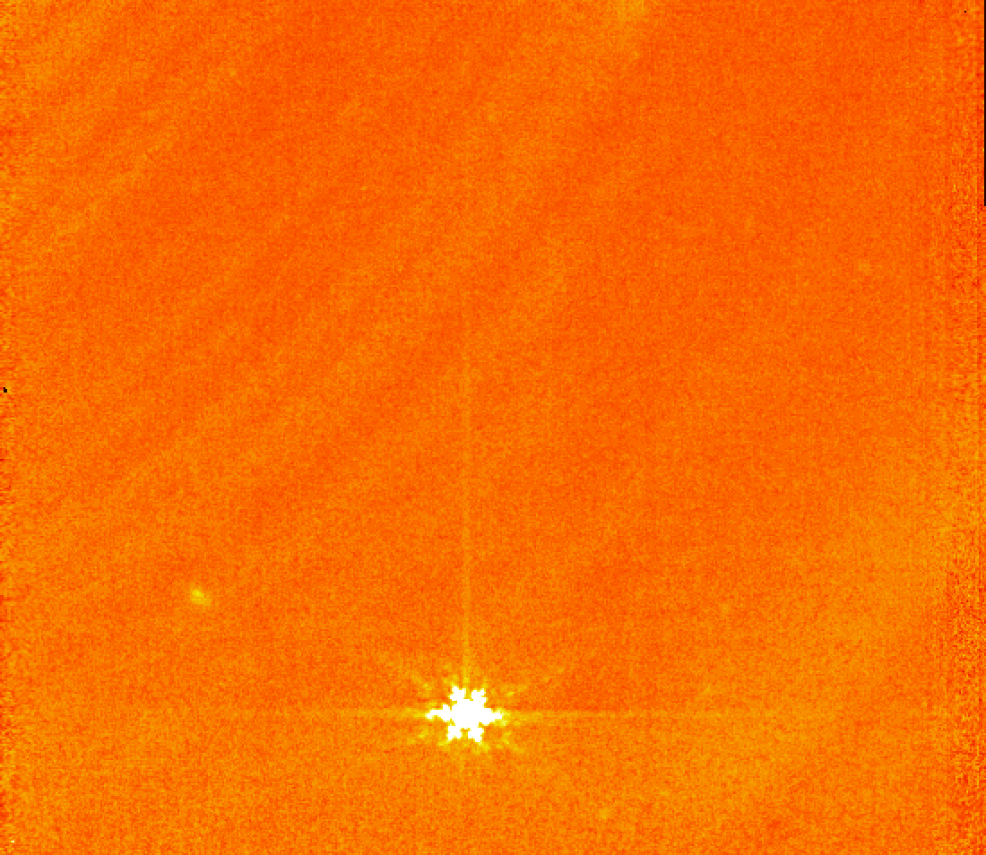
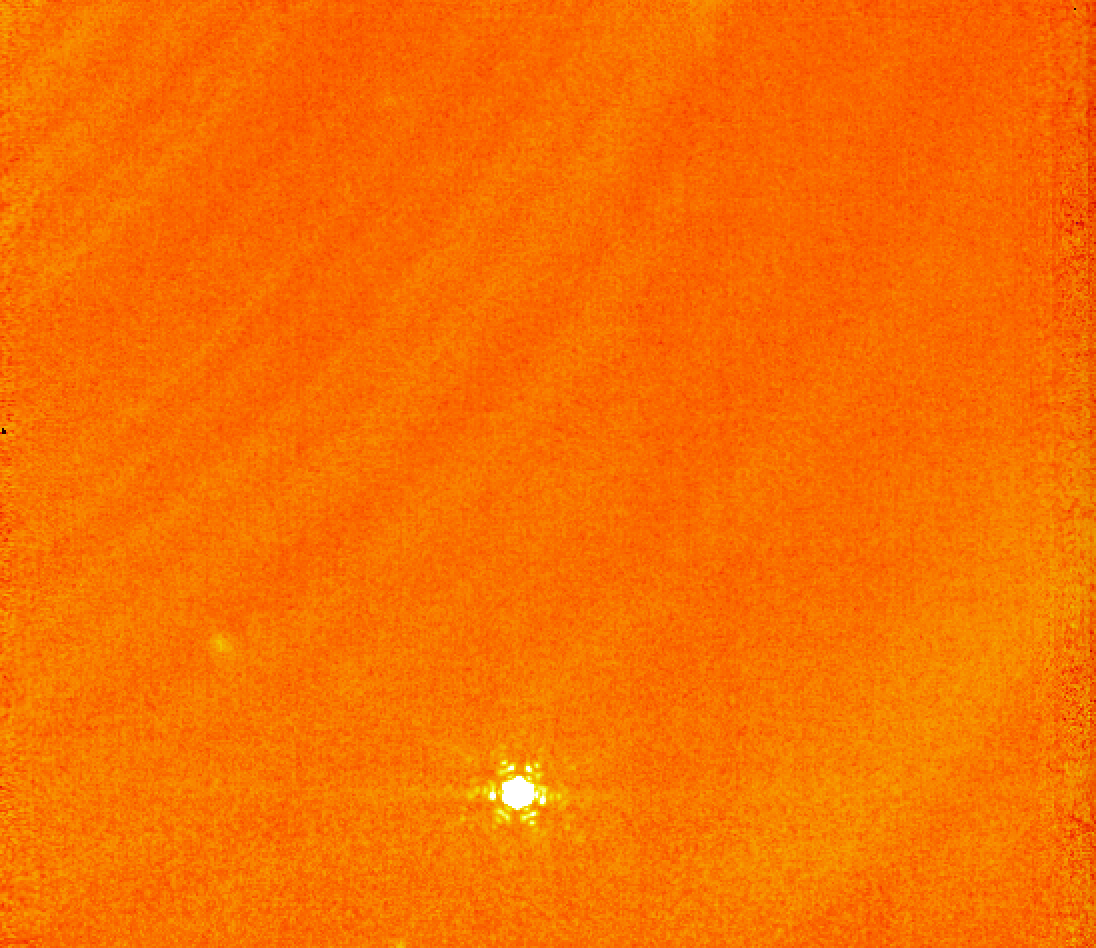
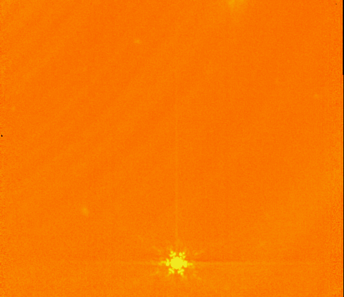
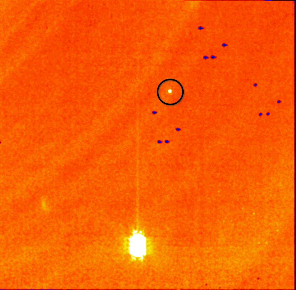
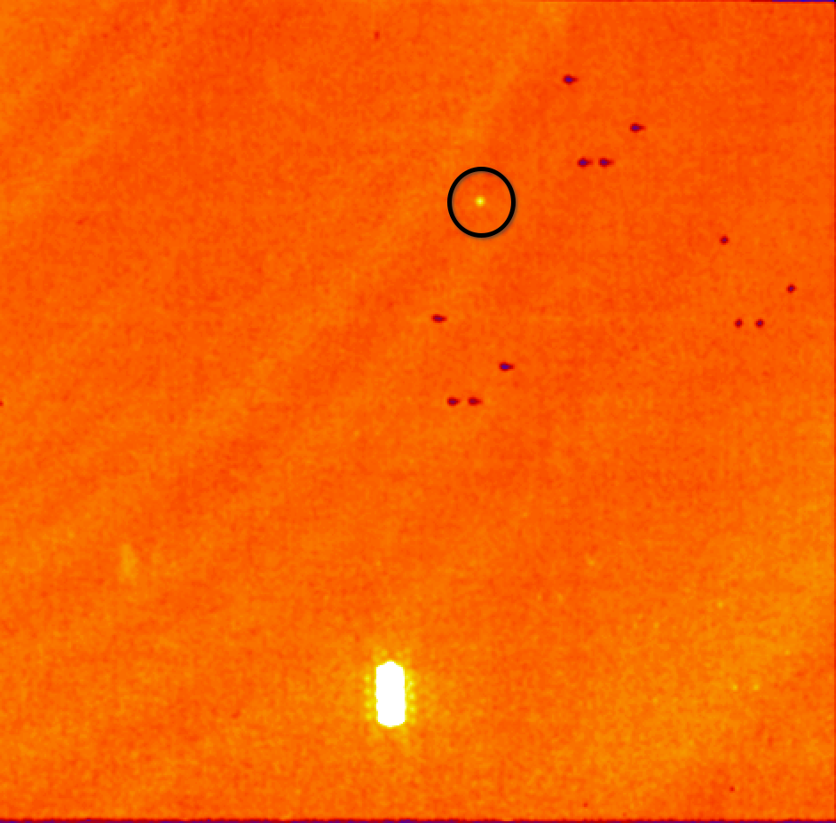
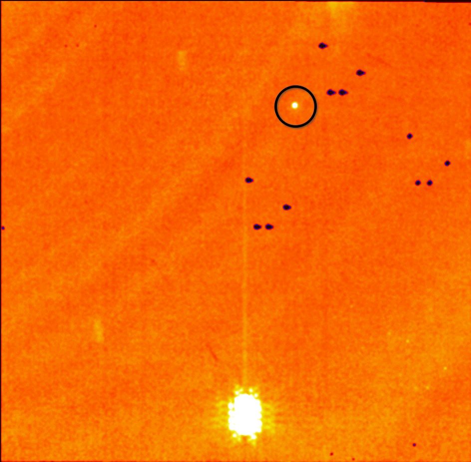
Figure 1: MIRI L3 images of asteroid (10920) (top row) in the F1000W, F1130W, and F1280W band (from left to right), and in the reference frame of (10920). The JWST-centric position of (10920) is 15h41m21.3s in R.A.  and -19^∘12^′17.0^′′, the FOV about 50^′′ $\times$ 40^′′. Bottom row: the corresponding L2 data in the same three bands, but the four dithered images in each band were manually stacked on the new faint asteroid (visible as faint point source in the upper part of the images, marked with a black circle). The FOV is about 50^′′ $\times$ 50^′′. The new object is not visible in the standard L3 data products in the archive.

2.2 Auxiliary observations and lightcurves for (10920)

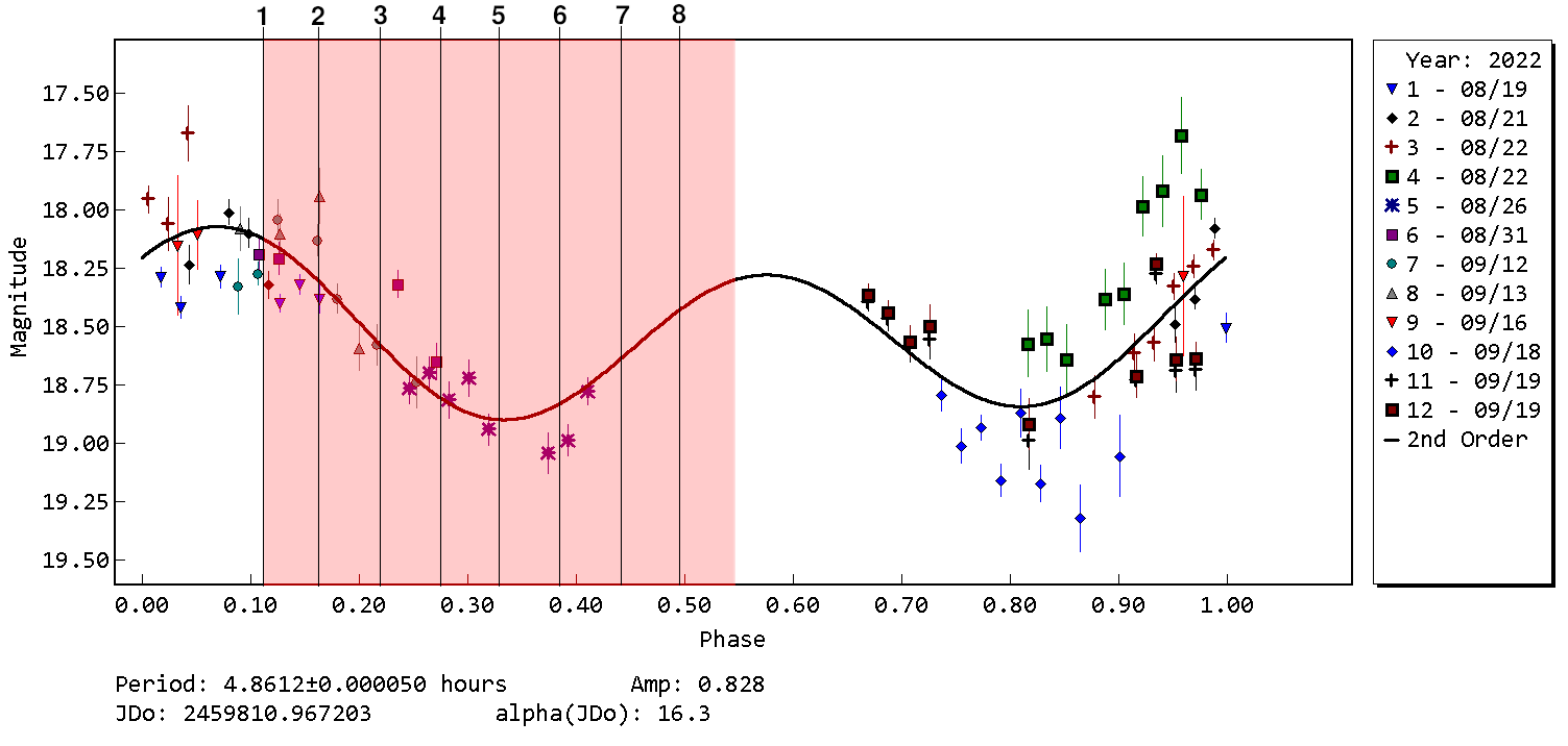
Figure 2: Lightcurve of (10920) obtained in July/August 2022. Using the period solution, the lightcurve (in the geocentric reference frame) has been phased to the MIRI observation epochs, which are marked with vertical black strokes indicating the beginning of each measurement. The numbers from 1 to 8 correspond to the lines in Table 3.

Although asteroid (10920) was discovered in 1998, there is very little knowledge about its physical properties. No shape model or full lightcurves are available, meaning that the spin state of the body is unknown. Since the asteroid’s shape and orientation are needed to refine the radiometric model, we performed an observation campaign from August to September 2022 to obtain a lightcurve of (10920) (see Figure 2). We used the 2 m telescopes of the Las Cumbres Observatory network: the Faulkes Telescope North (FTN) located at Haleakala Observatory and the Faulkes Telescope South (FTS) at Siding Spring observatory. All lightcurve data has been submitted to LCDB and can be retrieved by searching for ”10920”. Figure 2 shows the relevant measurements together with their photometric errors. The scatter between the photometric points is not fully compatible with the photometric errors. However, the viewing geometry changed slightly over the 32 days of measurements (phase angle range from 16.4^∘ to 15.0^∘). Therefore, the scatter on the composite lightcurve for observations taken some weeks apart is reasonable and expected for this very elongated object. The lightcurves are close to a sinusoidal function and show a large amplitude (larger than one magnitude in some cases) and a spin period of about 4.86 h. In order to study the spin shape and orientation we used a modified version of the SAGE modelling technique (Bartczak & Dudziński, 2018) to fit our lightcurve combined with the 13 available Gaia DR3 sparse photometric measurements of (10920) (Tanga et al., 2022). We used a simple triaxial ellipsoid shape to fit the data, since the number of measurements is not enough to study detailed shape features. However, this simple shape model has proved to work very efficiently to fit sparse data like the one provided by Gaia (Cellino et al., 2015), and also combined with ground-based lightcurves (Santana-Ros et al., 2015). We found a solid pole solution with $\lambda_{ecl}=178^{\circ}$ and $\beta_{ecl}=81^{\circ}$ (with an estimated error of about 20^∘), and a very elongated shape with axis ratios of $a/b=1.5-1.8$ and $b/c=1.0-1.1$. The Gaia and WISE (see Section 2.3 and Figure 10) data are best matched by a/b $\approx$ 1.5 while groundbased data pointed to an even more extreme elongation of the object. The SAGE lightcurve inversion (including the fit to the Gaia DR3 data) also resulted in a well-determined rotation period of 4.861191 $\pm$ 0.000015 h. From the spin solution we can infer that the object is always observed close to an equator-on viewing geometry, meaning that the aspect angle will not change much from apparition to apparition. Therefore, changes in the observed cross section of the object are mainly dominated by the a/b axis ratio while the object is rotating. We used the derived simple ellipsoidal spin-shape solution to phase the lightcurve (Fig. 2) back to the epoch of MIRI observations of (10920) (14 July 2022). The phased lightcurve shows that MIRI observations were obtained mainly during the minima, implying that most of the measurements were gathered close to the smallest possible cross section of the body, only the long-wavelength bands were taken at higher brightness approaching lightcurve maximum.

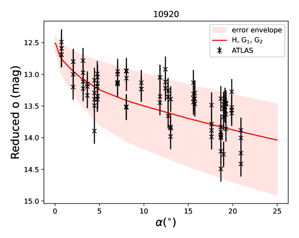
Figure 3: Fitting the H, G1, G2 photometric phase function to o-band data from the ATLAS survey obtained during three oppositions (2018, 2019/2020, 2021). The single-point uncertainty was assumed to be 0.2 mag.

For the determination of the H-magnitude of (10920) we fitted the H, G1, G2 photometric phase function of Muinonen et al. (2010) to the data from the ATLAS survey (Tonry et al., 2018). We utilized only the photometry from the orange filter as it was more numerous and had a better phase angle coverage than the data from the cyan filter. The orange passband ($\approx$550 - 820 nm) largely covers the Johnsons V band ($\approx$500 - 700 nm) and derived H values are very similar Photometry was downloaded through an astroquery wrapper for querying services at the IAU Minor Planet Center (MPC) (Ginsburg et al., 2019). Since the aspect changes between the oppositions are minimal, we fitted the data from three oppositions (2018, 2019/2020, 2021) together (see Fig. 3). The fit was performed in the flux domain using a linear least-squares procedure and we assumed 0.2 mag photometric uncertainty for the individual data points. Following Penttilä et al. (2016) we constrained the fits to obtain a physically meaningful solution: $H_{o}=12.51_{-0.12}^{+0.14}$ mag, and phase-function parameters $G_{1}=0.27_{-0.17}^{+0.21}$, $G_{2}=0.20_{-0.09}^{+0.08}$. This compares very well with values derived by Mahlke et al. (2021) and a previous study by Oszkiewicz et al. (2011).

2.3 Auxiliary WISE observations for (10920)

The Wide-field Infrared Survey Explorer (WISE, Wright et al., 2010) mapped in 2010 large parts of the sky in four IR bands at 3.4, 4.6, 12, and 22 $\mu$m (W1-W4). After the cryo-phase, the mission was continued as Near-Earth Object WISE (NEOWISE, Mainzer et al., 2014), but only in the short-wavelength channels W1 and W2. Masiero et al. (2011) published a size-albedo solution for (10920) based on multiple W3 (15x) and W4 (16x) detections. They found a size of 14.436 $\pm$ 0.267 km and a geometric albedo of p_V=0.0847 $\pm$0.0159 (based on H = 12.50 mag). The fitted beaming parameter $\eta$ is given with 1.058 $\pm$ 0.038. Nugent et al. (2015) published a size of 11.12 $\pm$ 2.85 km and p_V = 0.11 $\pm$ 0.07 (H=12.80 mag) as their best solution (via NEATM $\eta$-fit with $\eta$ = 0.95 $\pm$ 0.17). Detections from W1 (6x) and W2 (6x) were used for these calculations. They also see a 0.31 mag amplitude of the WISE 4.6 $\mu$m (W2) lightcurve, however, based on 6 data points only. Mainzer et al. (2019) list another solution where the fit was done on W2 (9x), W3 (9x), and W4 (10x) detections: D=15.712 $\pm$ 0.187 km, p_V = 0.082 $\pm$0.012, $\eta$ = 1.087 $\pm$ 0.022. All WISE-specific radiometric solutions are based on the Near-Earth Asteroid Thermal Model (via NEATM, Harris, 1998) which uses the beaming parameter $\eta$ to obtain the best fit to the observed spectral slope. $\eta$ depends on the object’s rotation, thermal, surface, and emissivity properties, and is also influenced by the observed wavelength regime and observing geometry (heliocentric distance and phase angle). The NEATM is closely connected to the Standard Thermal Model (STM, Lebofsky et al., 1986) which uses a fixed $\eta$ of 0.756, and which is widely applied to main-belt asteroids (e.g. Tedesco et al., 2002b, a; Delbo et al., 2015).

For our radiometric study of asteroid (10920), we extracted all W2, W3, and W4 WISE measurements with photometry quality flags ’A’ (SNR$\geq$10) or ’B’ (3$\leq$SNR$<$10), avoiding saturation, moon separation of less than 15^∘ or close-by background sources. The extracted magnitudes have been converted to fluxes (see Wright et al., 2010) and color-corrected with correction factors of 1.23, 0.97, and 0.98 for W2, W3, and W4, respectively. For the WISE absolute flux errors we considered the observational flux errors, an estimated error for the color correction and absolute flux errors which added up to minimum values of 15, 7, and 7% in the W2, W3, and W4 bands, respectively. The full list of WISE fluxes and errors are given in Table LABEL:app:wise_fluxes.

3 MIRI-related results

3.1 Astrometry

We determined the PSF centroid of asteroid (10920) (28 L2 images) and the newly discovered object (all 36 L2 images) by a simple 2-D Gauss fit, and used the WCS header information to translate the pixel coordinates into a rough estimate of their R.A. and Declination (see Table 2). The WCS-translated source positions gave a total apparent sky path of 7.27^′′ in 1:40:42.82 h or an apparent motion of 4.33^′′/h, in excellent agreement with JPL/Horizons predictions.

However, the absolute coordinates for (10920) are in poor agreement with the true JWST-centric ephemeris of the object, as determined by JPL/Horizons and our own orbital calculation. They show an offset of about 0.17^′′, which corresponds to about 1.5 pixels of the MIRI detector. The offset is not aligned with the direction of motion, and therefore not due to a timing issue.

In order to track down the source of this issue we manually re-measured the position of the asteroid in one of the shorter wavelength images, using stars that are visible in the IR image while still having counterparts in the optical. Unfortunately, only 2 Gaia DR3 sources are contained in the FoV of the MIRI frames. However, we located a deep optical image of the same area of the sky obtained by the Dark Energy Camera (DECam) (Flaugher et al., 2015) in their public archive. The frame, dated 2019 February 23, has an exposure time of 56 s, and contains a significant number of optical sources falling close to the MIRI sky-print. We carefully measured the position of 44 such sources versus a Gaia-based solution of the entire DECam chip, and used these positions to create a secondary catalog for applying to the astrometry of the MIRI frame. A total of 16 of such sources showed a detectable counterpart in the MIRI exposure, and could be used to perform a full astrometric solution on it, completely independent from the WCS coefficients. This solution evidenced a bias that exactly compensates the offset observed in the WCS-based astrometry. An astrometric measurement of asteroid (10920) with respect to this self-derived solution fits the existing ephemeris of the asteroid with residuals of $<$0.01^′′ in both coordinates (and has a formal uncertainty of roughly $\pm$0.03^′′). This test proves that the bias we observed in the WCS-based astrometry is due to the WCS solution present in the MIRI images, and it is not a manifestation of a physical offset in the object’s true sky position, nor of a problem with the ephemeris of the observing spacecraft.

Table 2: The WCS-based R.A. and Dec. coordinates of (10920) and the new object extracted from L2 products via Gaussian centroid fitting to the sources. MJD is the observation mid-time (UT).

		(10920) 1998 BC1		new object
No.	MJD	R.A. [deg]	Dec. [deg]	R.A. [deg]	Dec. [deg]
01	59774.431476	235.3396411	-19.2048876	235.3453320	-19.2049123
02	59774.433749	235.3395726	-19.2048763	235.3454998	-19.2049910
03	59774.436073	235.3395027	-19.2048649	235.3456712	-19.2050717
04	59774.438387	235.3394330	-19.2048534	235.3458419	-19.2051356
05	59774.441776	235.3393309	-19.2048367	235.3460921	-19.2052401
06	59774.443910	235.3392667	-19.2048262	235.3462495	-19.2053028
07	59774.446043	235.3392024	-19.2048156	235.3464069	-19.2053612
08	59774.448136	235.3391394	-19.2048053	235.3465613	-19.2054410
09	59774.451932	235.3390251	-19.2047865	235.3468414	-19.2055228
10	59774.454055	235.3389612	-19.2047760	235.3469981	-19.2055865
11	59774.456128	235.3388987	-19.2047658	235.3471510	-19.2056832
12	59774.458222	235.3388357	-19.2047555	235.3473055	-19.2057778
13	59774.461326	235.3387422	-19.2047401	235.3475346	-19.2058274
14	59774.463449	235.3386783	-19.2047296	235.3476912	-19.2059116
15	59774.465613	235.3386131	-19.2047190	235.3478509	-19.2059585
16	59774.467716	235.3385498	-19.2047086	235.3480061	-19.2060255
17	59774.470790	235.3384572	-19.2046934	235.3482329	-19.2061170
18	59774.472913	235.3383933	-19.2046829	235.3483896	-19.2061859
19	59774.475056	235.3383288	-19.2046723	235.3485477	-19.2062493
20	59774.477190	235.3382645	-19.2046618	235.3487051	-19.2063141
21	59774.480355	235.3381692	-19.2046462	235.3489387	-19.2064240
22	59774.482498	235.3381047	-19.2046356	235.3490968	-19.2064844
23	59774.484631	235.3380404	-19.2046250	235.3492542	-19.2065476
24	59774.486754	235.3379765	-19.2046145	235.3494109	-19.2066109
25a	59774.489829	—	—	235.3496377	-19.2067233
26	59774.491932	235.3378206	-19.2045890	235.3497929	-19.2067603
27	59774.494105	235.3377552	-19.2045782	235.3499533	-19.2068342
28	59774.496248	235.3376906	-19.2045677	235.3501114	-19.2069013
29b	59774.499293	—	—	235.3503361	-19.2069632
30	59774.501416	235.3375350	-19.2045421	235.3504927	-19.2070349
31b	59774.503539	—	—	235.3506494	-19.2070889
32b	59774.505622	—	—	235.3508031	-19.2071688
33b	59774.509208	—	—	235.3510677	-19.2073011
34b	59774.511411	—	—	235.3512302	-19.2073613
35b	59774.513604	—	—	235.3513921	-19.2074352
36b	59774.515738	—	—	235.3515495	-19.2074973

^a Asteroid (10920) at edge, no centroid position possible. ^b Asteroid (10920) is outside FOV.

The new object was detected in all 36 L2 frames (9 filters with 4 dithered frames in each band). The WCS-translated source positions are also given in Table 2. The new target moved by 23.00^′′ during the 2:01:20.24 hours, corresponding to an apparent motion of 11.37^′′/hour, or about 2.6 times faster than the outer main-belt asteroid (10920). We also determined the absolute astrometric solution for the new object based on the DECam deep optical image and connected to a Gaia-based solution, as described above for (10920). This allowed us to determine highly accurate ($<$ $\pm$0.05^′′) positions for the new object in the short-wavelength MIRI bands (where the stars are still visible). The observed arc is in principle too short for the MPC to designate it (it will be kept in the unpublished and unreferenced ”Isolated Tracklet File”), but future projects like LSST or the NEO Surveyor might be able to pick it up again. The JWST positions of this new object from July 2022 will then be very useful for orbit calculations.

3.2 IR Photometry

Before we worked on the flux extraction for both moving objects, we looked at all calibration stars which were observed as part of the MIRI photometric calibration program. They were taken in the same MIRI imaging mode, the same readout (FASTR1) and dither mode (4-POINT-SETS), and only the sub-array settings (SUB64, SUB128, SUB256, BRIGHTSKY, FULL) and the exposure times were different. These stars cover the MIRI flux range between 0.05 mJy (in F2550W) and above 300 mJy (in F560W), similar to the flux levels of the asteroid (10920). We applied aperture photometry (up to a point where the growth curve flattened out) with the sky background subtracted (calculated within an annulus at sufficient distance from the star, avoiding background sources and image artifacts). When comparing these aperture fluxes with the corresponding model fluxes (Gordon et al., 2022), we found an agreement of typically 5% or better, but with some outliers on the 10-15% level, mostly in cases where the star was close to the edge of the FOV or near a bright artifact (visible in level-2 products). Only for HD 2811, we found MIRI fluxes (level-2 and level-3 products) which are about 1.5-2.2 times higher than the model fluxes. The reason for the HD 2811 discrepancy is not clear, but Rieke et al. (2022) flagged this star as less reliable due to obscuration (A_V $>$ 0.2 mag). We excluded this star from our study.

Following the experience from our stellar calibration analysis, we performed similar aperture photometry for the two moving objects, both on L2 and L3 data (or manually stacked level-2 frames for the new object). For the flux error we considered the scatter between the individual L2 fluxes and the SNRs of the combined images. In case of (10920), the SNRs are well above 100 in all cases and the scatter between fluxes derived from the four L2 frames agree within 5%. Therefore, we took 5% as the measurement error, except for the single F2100W measurement where a significant part of the source PSF is outside the FOV. Here, we performed a ”half-source photometry” (multiplied by 2) and we estimated a 10% measurement error.

For the new object the fluxes are much lower (note, that we use mJy for (10920) and $\mu$Jy for the new object!). Still, the SNR for this object ranges between 10 and 20 (individual L2 frames) and goes to 25 in some of the final stacked images. At longer wavelengths, the object increases in brightness, but also the background level goes up, and the detection was more difficult.

The MIRI flux calibration is based on the assumption of ${F}_{\mathrm{ref}}(\lambda)=\mathrm{const.}$ (Gordon et al., 2022). It is therefore necessary to color-correct the extracted in-band fluxes to obtain mono-chromatic flux densities at the MIRI reference wavelengths. Based on the MIRI filter transmission curves and a WISE-based model spectrum for (10920) (Mainzer et al., 2019), we calculated corrections factors of 1.15, 1.02, 0.99, 1.00, 0.99, 0.99, 1.00, 1.01, and 1.01 in the 9 MIRI bands from F560W to F2550W (roughly corresponding to the corrections for $\approx$200-240 K black bodies). For the color correction we assume a 2% error (5% in the F560W band), and for the MIRI absolute flux calibration another 5% error in all bands. All errors were added quadratically. The results are presented in table 3 and in Figures 4 and 5. Note that these multi-band fluxes cannot be used to see rotational (lightcurve) flux variations directly as the flux changes are dominated by the change in wavelength. Only in combination with good-quality spin-shape model solutions there is a possibility to (partially) separate rotational from spectral flux variations (see discussion for (10920) in Section 4).

Table 3: Extracted MIRI fluxes for the main-belt asteroid (10920)^a (in mJy) and the new faint asteroid^b (in $\mu$Jy).

. MBA (10920) New Object No. MJD $\lambda$ [$\mu$m] flux [mJy] error^c [mJy] Comments flux [$\mu$Jy] error^c [$\mu$Jy] Comments 1 59774.434921 5.60 0.40 0.03 L2 1-4 & L3 4.0 1.1 low SNR 2 59774.444966 7.70 3.89 0.27 L2 5-8 & L3 25.9 3.4 3 59774.455084 10.00 13.19 0.90 L2 9-12 & L3 54.3 5.7 4 59774.464526 11.30 20.14 1.48 L2 13-16 & L3 79.7 9.0 5 59774.473988 12.80 25.67 1.63 L2 17-20 & L3 93.5 8.3 6 59774.483560 15.00 35.83 2.15 L2 21-24 & L3 121.3 7.5 7 59774.493029 18.00 54.31 3.98 L2 26-28 & L3 103.1 8.3 high bgr 8 59774.502468 21.00 77.63 8.79 L2 30 & L3 91.8 24.4 high bgr 9 59774.512490 25.50 — — out of FOV 111.2 19.8 high bgr

^a The asteroid (10920) was at a helio-centric distance of r=3.5640 au, a JWST-centric distance of 2.86328 au, a solar elongation of 125.87^∘, and seen under a phase angle $\alpha$=13.51^∘ at observation mid-time (2022-Jul-14 11:20 UT). ^b For the faint new asteroid, only its positions over two hours and the apparent motion are known (see Table 2). Both objects had a solar elongation ($\lambda$ - $\lambda_{sun}$) = 125.8^∘, as seen from JWST. ^c The flux errors are standard deviations of the photometry of the four level-2 images, combined with estimated errors for the color correction and absolute flux calibration.

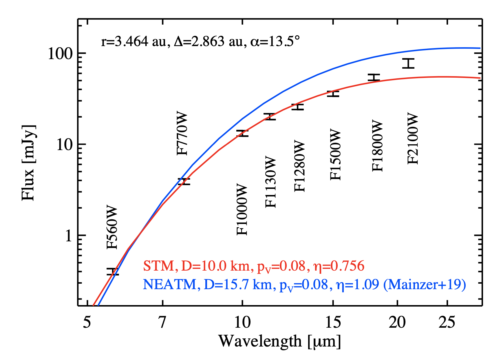
Figure 4: The extracted MIRI fluxes for asteroid (10920), shown together with two different model predictions for the JWST observing epoch and geometry. The blue line shows the NEATM prediction, using the (Mainzer et al., 2019) solution, the red line is based on a STM prediction, but using a 10 km diameter for (10920).

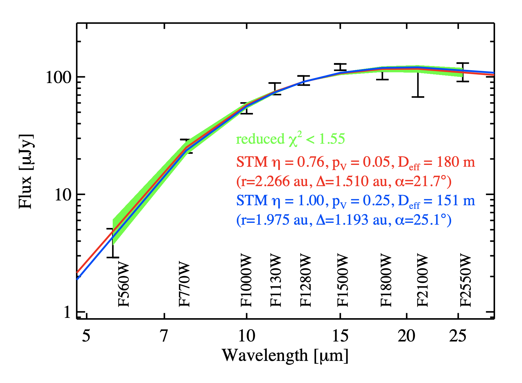
Figure 5: The extracted MIRI fluxes for the new object, shown together with STM predictions for two different $\eta$-values which correspond also to different best-fit $r,\Delta,\alpha$ observing geometries. The red line shows the $\eta=0.756$ (p_V = 0.05, D_eff = km), the blue line the $\eta=1.0$ (p_V = 0.25, D_eff = km) STM solution, and the green envelope all orbit solutions with $\chi^{2}$ $<$ 1.55. Note that the flux scale is given in $\mu$Jy.

4 Radiometric study for MBA (10920)

Figure 4 shows our calibrated MIRI fluxes of MBA (10920) together with two flux predictions: (1) A NEATM prediction (blue line) for this specific JWST-centric observing geometry on July 14, 2022. The model parameters (D, p_V, and $\eta$) were taken from Mainzer et al. (2019). (2) In addition, we calculated a STM prediction ($\eta$=0.756) for a 10 km diameter sphere (with p_V=0.082 as in the NEATM calculations) shown in red. The NEATM fluxes are too high (by almost a factor of 2 at 15 $\mu$m) while the STM fluxes are in nice agreement in the wavelength range up to 18 $\mu$m. Only the 21 $\mu$m point is off, but it was taken when the source was at the edge of the MIRI array. And, as can be seen from Figure 2, the 21 $\mu$m point (No. 8 in Table 3) falls close to the lightcurve maximum which might also explain the discrepancy with the simple model prediction.

The 8 MIRI fluxes (or only 7 as the 21-$\mu$m flux is uncertain) span a wide wavelength range close to the object’s thermal emission peak. We fitted these data with the STM by using different beaming values (and albedos). A beaming parameter of $\eta$ = 0.76 ($\pm$ 0.03) (or 0.73 $\pm$ 0.04 when using 7 fluxes only) produces the best-fit to the observations. In conclusion, the STM assumption with $\eta$=0.756 is working very well in case of our MIRI observations of (10920). The corresponding STM radiometric size is 10.0 $\pm$ 0.2 km, the geometric albedo 0.13 (assuming an absolute magnitude H = 12.8 mag).

The WISE data were taken in mid January 2010 (11 detections in W3/W4) at a phase angle of +18.8^∘ (trailing the Sun) and in early July 2010 (14 detections in W3/W4) at a phase angle of -17.9^∘ (leading the Sun). These dual-band and dual-epoch data are best fit for a pro-grade spin of (10920) with a thermal inertia in the range between 9 and 35 J m^-2s^-0.5K^-1, with the best-fit value of 15 J m^-2s^-0.5K^-1. The WISE flux variations point to an elongated body with an estimated axis ratio a/b $\approx$ 1.5 (see Fig. 10). However, a simple ellipsoidal shape cannot fully explain the observed thermal lightcurves. Instead, the variations might point to a (contact-)binary system. The relatively high thermal inertia (as compared to other outer main-belt objects, see Delbo et al. (2015)) leads to a radiometric size of 14.5 - 16.5 km (size of an equal-volume sphere), larger than our STM predictions and close to previously published WISE solutions. The best-fit radiometric size for a spherical shape model is 14.7 km, the best-fit for the ellipsoidal shape is a bit larger at 15.3 km. Based on the WISE-W3 and W4 data (Fig. 10), we estimated a minimum cross section of (10920) of about 10.5 km (similar to our initial STM fit to the JWST data in Fig. 4), and a maximum cross-section of 18 km. However, the MIRI observations were taken close to the lightcurve minimum (see Fig. 2) and a radiometric TPM analysis of these data alone would result in a smaller cross-section (about 11-13 km in diameter). Adjusting the MIRI fluxes via our optical lightcurve data to a lightcurve-median value (followed by a radiometric study using a spherical-shape model) is not easily possible. Lightcurves are changing with phase angle and, the interpretation in terms of spin-shape properties depends on surface scattering models (Lu & Jewitt, 2019). The IR fluxes, on the other hand, are influenced in a wavelength-dependent fashion by thermally-relevant properties, like the surface roughness or thermal inertia (Müller, 2002). Only at longer wavelengths, close to the thermal emission peak and beyond, the thermal fluxes are less sensitive to thermal properties and follow closely the object’s changes in cross section. A simple (optical) lightcurve-based correction of the MIRI fluxes is therefore not possible.

The object’s albedo is connected to the absolute magnitude. H = 12.5 mag corresponds to p_V = 0.07, as expected for a typical object in the outer main-belt region. A smaller (larger) H-magnitude would lead to a higher (lower) albedo and p_V values between 0.05 and 0.09 are compatible with the available absolute magnitude fits (see Fig. 3).

5 STM-ORBIT method

In this section, we assume that the orbits of both asteroids are not known. The goal is to constrain the size, helio-centric distance (at the same time the JWST-centric distance $\Delta$ and the phase angle $\alpha$), and possibly also their orbital parameters by just using the MIRI fluxes, the JWST-centric R.A. and Dec. coordinates, the derived apparent motion, and the solar-elongation of the targets at the time of the MIRI measurements.

5.1 Orbit calculations

For the MBA (10920) we calculated more than 9300 orbits that are compatible with the observed JWST-centric RA/Dec and motion direction of the object, the apparent solar elongation, and the specific apparent motion of 4.33^′′/hour. The calculations were done via a ranging approach (Virtanen et al., 2001; Oszkiewicz et al., 2009) using the ”Find_Orb” software. Similar ranging computations have been used before, but usually in the context of unconstrained systematic ranging concepts for the orbit determination of near-Earth asteroids, for impact probability calculations or collision predictions (e.g. Virtanen & Muinonen, 2006; Oszkiewicz et al., 2012; Farnocchia et al., 2015). These orbits cover a wide parameter space with semi-major axes between 0.6 and 1000 au, eccentricities between 0.0 and 1.0, inclinations between 0 and 180^∘, and perihelion distances are from 0.008 to 29 au. All of these orbits can explain the MIRI-specific astrometric data presented in Tbl. 2 within assumed uncertainties of $\pm$0.025^′′ and $\pm$0.050^′′ respectively for the two objects, with a reduced $\chi^{2}$ of the orbital fit being close to unity.

For the new asteroid, a similar procedure was applied, this time for the specific apparent motion of 11.37^′′/hour. The almost 10 000 orbits cover a similar parameter space as the ones for (10920), but due to the different motion of the arc observed in the sky, the orbit ranging approach constrained the orbital perihelia to values below 3.3 au.

Each of the possible orbit solution is coming with orbital parameters $a$ (semi-major axis), $e$ (eccentricity), $i$ (inclination), $q$ (perihelion distance), and the calculated $r_{helio}$ (helio-centric distance [au] from the Sun), $\Delta$ (JWST-asteroid distance [au]), and $\alpha$ (phase angle in [^∘]) for the specific JWST observing geometry and observing epoch.

5.2 STM calculations and fit to the MIRI data

The possible orbit solutions are now taken to calculate flux predictions at the MIRI reference wavelengths, and by using the corresponding $r_{helio}$, $\Delta$, and $\alpha$ values. The model calculations are done via the STM, but with the option to use different values for the beaming parameter $\eta$. A 1-km diameter is used as a starting value and predictions are done for a range of different albedos (p_V = 0.05, 0.10, 0.15, 0.20, and 0.25). In a second step, the reference diameter is scaled up or down to obtain the best fit in terms of $\chi^{2}$-minimization to the MIRI fluxes: The $\chi^{2}$ calculation is done via $\sum\frac{(flx_{miri}(i)-flx_{STM}(i))^{2}}{{\sigma}(i)^{2}}$, with $flx_{miri}$ and $\sigma$ being the individual MIRI fluxes and absolute errors (see Table 3), and $flx_{STM}$ the corresponding STM prediction. This recipe produced for each orbit (and each albedo value) the best-fit size solution and the corresponding (reduced) $\chi^{2}$ value.

5.3 MBA (10920)

The $\chi^{2}$ fitting for (10920) was done for all 8 fluxes from 5.6 to 21.0 $\mu$m (see Tbl. 3), with $\mu=n-m=7$ as the degree of freedom (considering the diameter scaling as the only fitting parameter $m$). The 21-$\mu$m point is not well matched by our spherical STM shape model. The reason could either be the fact that (10920) was partially outside MIRI’s FOV and the photometry is simply wrong, or spin-shape related problems (see Section 2.2). Therefore, we did a separate $\chi^{2}$ fitting for the 7 good-quality fluxes (from 5.6 to 18.0 $\mu$m), and with $\mu$ = 6 as the degree of freedom for the reduced $\chi^{2}$ calculations. The results are shown in Fig. 6.

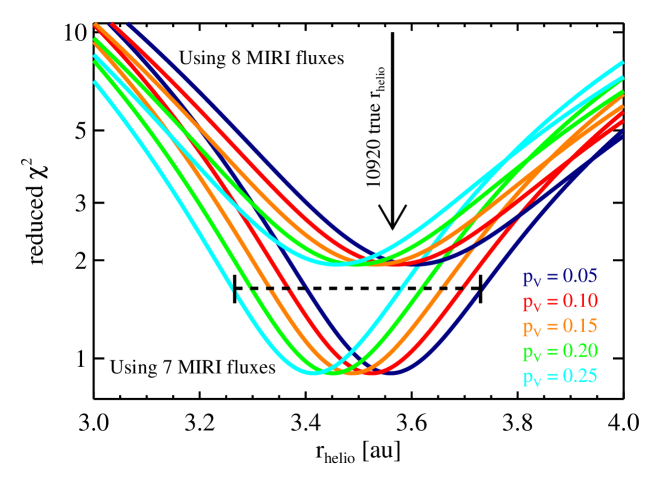
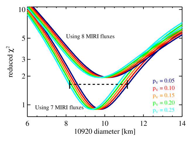
Figure 6: Results of the $\chi^{2}$-fitting of STM predictions to the measured MIRI fluxes of asteroid (10920). Top: Assuming that the orbit of (10920) is not known, we find that the most likely r_helio would be in the range between 3.25 and 3.75 au. Bottom: The most-likely size, based on the MIRI data alone and assuming a spherical shape of (10920), would be in the range between 8 and about 11.5 km.

The STM-ORBIT method puts very strong constraints on the object’s helio-centric distance at the time of the JWST observations: 3.27 au $<$ r_helio $<$ 3.73 au, where the lower (higher) boundary is connected to the assumption of a high (low) albedo of p_V = 0.25 (0.05). This places the object at the edge of the outer main-belt at the time of the JWST observations. In a similar way, the JWST-object distance is limited to 2.56 au $<$ $\Delta_{JWST}$ $<$ 3.04 au, and the phase angle $\alpha$ to values between 13.0 and 14.9^∘. These derived radiometric distance and angle ranges for (10920) 1998 BC1 are in excellent agreement with the true values r_helio = 3.56 au, $\Delta_{JWST}$ = 2.86 au, $\alpha$ = 13.5^∘ at 2022-Jul-14 11:30 UT.

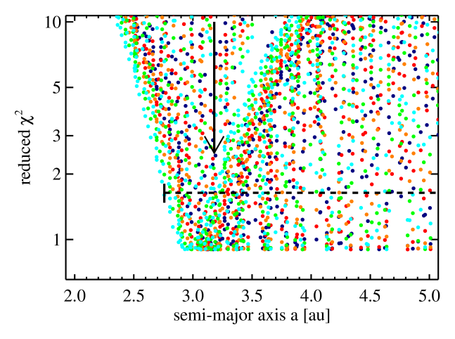
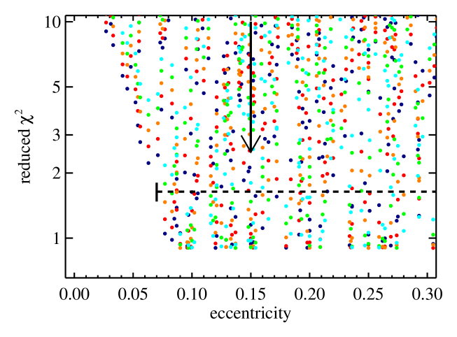
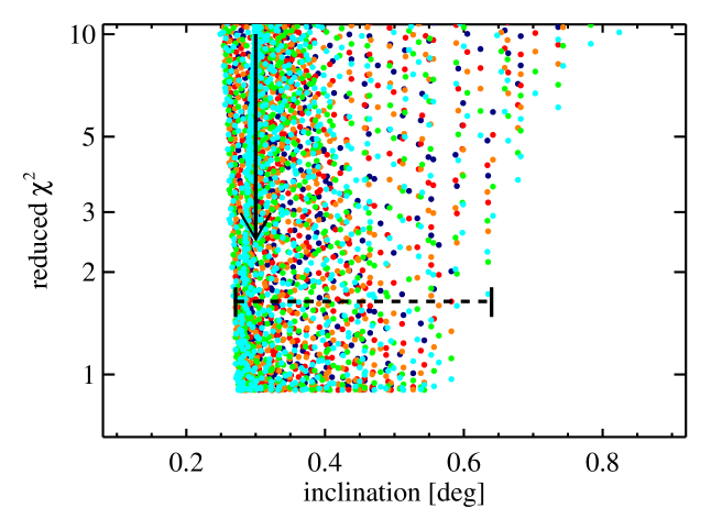
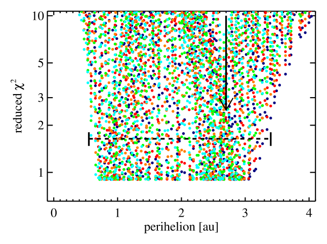
Figure 8: Orbit constraints from the $\chi^{2}$-fitting of STM predictions to the measured MIRI fluxes of asteroid (10920). From top to bottom: (i) Semi-major axis $a$; (ii) eccentricity; (iii) inclination; (iv) perihelion distance. The true values for (10920)’s orbit are indicated by a vertical arrow. The possible ranges are shown at reduced $\chi^{2}=1.64$ (6 degrees of freedom).

It is interesting to see that the small observed arc combined with the MIRI fluxes also limit the possible orbital parameters $a$, $e$, $i$, and $q$ (see Fig. 8): the orbit’s semi-major axis $a$ has to be larger than 2.76 au (true value: 3.18 au), the eccentricity $e$ larger than 0.07 (0.15), the inclination $i$ between 0.27^∘ and 0.64^∘ (0.30^∘), and the perihelion distance between 0.55 au and 3.40 au (2.70 au). This is clearly not sufficient for an orbit determination, but makes a classification as an outer main-belt object very likely. It seems, we can also exclude highly eccentric orbits ($e$ $>$ 0.99) with semi-major axes larger than about 100 au, but here our orbit statistic was not sufficient for a solid confirmation.

But the strongest point of the STM-ORBIT method is the size determination. Without knowing the object’s true orbit, it is possible to estimate an effective size between 8.2 and 11.2 km, with the smaller value being connected to p_V = 0.25 and the larger one to p_V = 0.05. The STM-related size is smaller than the radiometric TPM size (see Section 4), but this is mainly related to the spherical shape (as compared to the extremely elongated shape in the TPM study) and the fact that JWST caught (10920) during the lightcurve minimum when its cross section is minimal. Constraining the asteroid’s albedo is not possible, as a bright and large object can produce the same thermal emission as a dark but smaller body.

5.4 New asteroid

The $\chi^{2}$ fitting for the new object was done for all 9 fluxes from 5.6 to 25.5 $\mu$m (see Tbl. 3), with $\mu=n-m=8$ as the degree of freedom. The STM-ORBIT method with $\eta$ = 0.756, as it was used and verified for the outer MBA (10920), revealed that the new object must be located at a heliocentric distance of about 2.0 - 2.5 au. As smaller objects located closer to the Sun tend to have larger beaming values (see, e.g., discussions in Alí-Lagoa et al. (2016); Alí-Lagoa & Delbo’ (2017)), we also used $\eta$ = 1.0. It turned out that both $\eta$-values can fit the 9 fluxes equally well, but the related best-fit helio-centric distances differ (see Fig. 7). For constraining the object’s size, location and orbit, we therefore used the full $\eta$-range from 0.76 to 1.0. Two extreme solutions are shown in Fig. 5: a dark (p_V = 0.05, D_eff = 180 m) object at large heliocentric distance of r_helio = 2.266 au (as red solid line) with a model beaming parameter $\eta$ = 0.76, and a bright object (p_V = 0.25, D_eff = 151 m) at r_helio = 1.975 au (solid blue line), but with a beaming parameter of 1.0. Both solutions fit nicely the MIRI fluxes. All $\chi^{2}$-compatible solutions (here, for reduced $\chi^{2}$ values of 1.55) are indicated by the green lines.

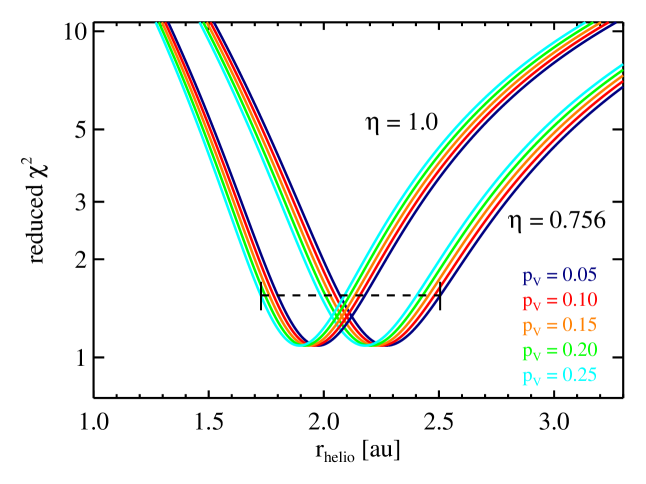
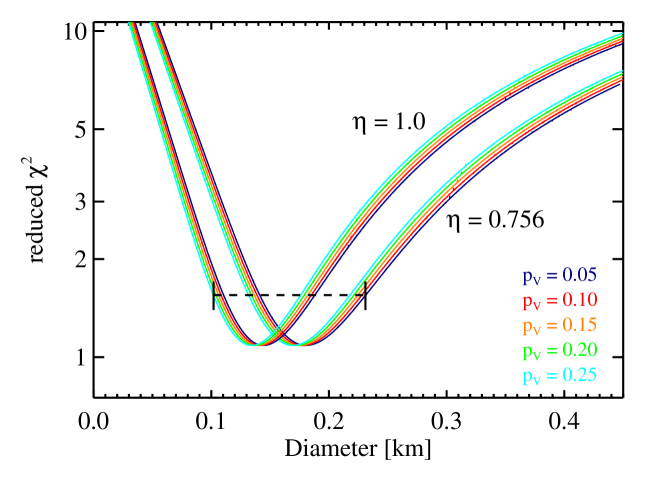
Figure 7: Results of the $\chi^{2}$-fitting of STM predictions to the measured MIRI fluxes of the new object. The triangles are related to a beaming parameter of $\eta$ = 1.0, the diamonds belong to $\eta$ = 0.756. Top: We find that the most likely r_helio would be in the range between 1.95 and 2.55 au. Bottom: The most-likely size, based on the MIRI data and assuming a spherical shape, would be in the range between 100 and about 230 m.

The nine MIRI fluxes can then be explained best if the new object is located at 1.73 au $<$ r_helio $<$ 2.50 au, 0.91 au $<$ $\Delta_{JWST}$ $<$ 1.76 au, 19.2^∘ $<$ $\alpha$ $<$ 29.0^∘. The orbital parameters are restricted to $a$ $>$ 1.3 au, $e$ $>$ 0.01, 0.7^∘ $<$ $i$ $<$ 2.0^∘, and 0.1 au $<$ $q$ $<$ 2.50 au. This gives a high probability for a low-inclination, inner main-belt object. The size of this newly discovered small body is between 100 m and 230 m in diameter where the smallest value is connected to $\eta=1.0$ and high albedo, the largest size to $\eta=0.756$ and a dark albedo. A wide range for the beaming parameters $\eta$ would broaden the parameter range, but due to the very-likely inner main-belt location (coming with moderate phase angles below 30^∘) justifies the applied beaming range. However, an even larger beaming value cannot be excluded and the object would fall into the sub-100 m category, with the heliocentric distance approaching 1.5 au. We also applied the STM-ORBIT method to a reduced observational data set. With less and less data, the $\chi^{2}$ goes down and broader and broader parameter ranges (for r_helio, D_eff) are compatible with the observations. E.g., without the 5.6 $\mu$m data point the possible distance from the Sun would slightly decrease to 1.65 au, at the same time, the connected diameter of the new object would shift to 80-220 m. It is therefore essential for the success of the STM-ORBIT method to have detections in the widest possible wavelength range available.

6 Discussion

Our STM-ORBIT method can locate the position ($r_{helio}$, $\Delta$, $\alpha$) of an unknown object and distinguish between a near-Earth object, inner-, middle-, outer main-belt, or an object beyond the main belt. Depending on the length of the observed arc, also the orbit inclination can be derived, and strong limitations of the possible perihelion distances can be given. For $a$ and $e$ the method allows to exclude some extreme cases. However, the big advantage is the radiometric size determination without knowing the object’s true orbit. The main uncertainty is related to the poorly constrained beaming parameter $\eta$ and the degeneracy between the object’s heliocentric distance and the applied model beaming parameter (see Figs. 5 and 7). As a starting point, we used the STM-default value of $\eta=0.756$ (Lebofsky et al., 1986). This is also the best-fit value for (10920) when we use the object’s true distances and angles (see Section 4). Masiero et al. (2011) used a huge WISE database to determine the beaming parameter of main-belt asteroids as a function of phase angle $\alpha$: $\eta$ = (0.79 $\pm$ 0.01) + $\alpha$(0.011 $\pm$ 0.001), however, with a very large scatter of values between 0.6 and about 2.0. The formula would lead to an $\eta$-value close to 0.95 for (10920) which is too high for our MIRI fluxes. The high-SNR AKARI asteroid measurements (Usui et al., 2011) led to a slightly different correlation of $\eta$ = (0.76 $\pm$ 0.03) + $\alpha$(0.009 $\pm$ 0.001) (Alí-Lagoa et al., 2018) and about 5% lower beaming values for our case here. Grav et al. (2012) found for the more-distant Hilda group $\eta$ = 0.85 $\pm$ 0.12. As the beaming parameter is also influenced by the covered wavelength range (with respect to the object’s thermal emission peak), and based on the fit to the (10920) MIRI fluxes, we considered the default STM value a solid starting point for a ”blind” interpretation of MIRI data. For the maximum of $\eta$ we used 1.0, compatible with the above mentioned published correlations for typical small-size main-belt objects. However, if an object turns out to be closer to the Sun and/or observed under much larger phase angles, then also larger $\eta$-values have to be considered for the STM-ORBIT method.

For a successful application of the STM-ORBIT method it is also mandatory that the measurements cover a wide wavelength range, or more specific, that the measurements allow to estimte the object’s temperature (in the STM context: the sub-solar temperature T_SS). Already a restriction to the first 5 filters from 5.6 to 12.8 $\mu$m would make the temperature determination more uncertain and enlarge the possible size solutions by almost a factor of 2. And, the object location could be anywhere within the main-belt. Future projects, like the NEO Surveyor (Mainzer et al., 2015) plan to measure only in two bands at 4-5.2 $\mu$m and 6-10 $\mu$m. A similar STM-ORBIT application for newly discovered objects would then only work when multiple, time-separated detections in both bands are available.

The unprecedented sensitivity of MIRI will guarantee that many small asteroids will be detected. A powerful method to find and extract moving targets from the MIRI imaging data will be the ESASky tool (Racero et al., 2022). The STM-ORBIT method will allow to determine basic properties and put constraints on their orbits. This is needed in the context of asteroid size-frequency distribution (see e.g., Bottke et al., 2005, 2015a). Tedesco & Desert (2002) used the ISO satellite (Kessler et al., 1996) to obtain a deep asteroid search at 12 $\mu$m in the ecliptic plane. They estimated a cumulative number of MBAs with diameters larger than 1 km between 0.7 and 1.7 million objects. However, the authors also stated that different statistical asteroid models differ already by a factor of two at the 1 km size limit while at 2 km sizes they are still in good agreement. The MBA statistics at a size range well below 1 km remains unknown. A Spitzer (Werner et al., 2004) study by Ryan et al. (2009, 2015) looked into the 0.5 - 1.0 km diameter asteroid population at different ecliptic latitudes $\beta$ between -17^∘ and +15^∘. Their IR measurements indicated that the number densities are about a factor of 2-3 below predictions by a Standard Asteroid Model. However, they speculated that the limiting magnitude of current asteroid surveys might have caused the offset. Masiero et al. (2011) presented sizes and albedos of more than 100 000 MBAs derived from the WISE/NEOWISE surveys at thermal IR wavelengths. But with very few exceptions, the derived sizes are above 1 km. The mean beaming parameter $\eta$ was found to be about 1.0, ranging from $\approx$ 0.94 for small phase angles to values above one at high phases (see also our discussion above about the selection of $\eta$ for our two targets). They confirm a bimodal albedo distribution, and decreasing average albedos when going from the inner main belt to outer regions. But due to the WISE detection limits, the sub-kilometer MBA regime could not be characterized. A recent asteroid study with the Hubble Space Telescope (Kruk et al., 2022) found about 60 asteroids per square degree with magnitudes brighter than 24.5 mag in a 30^∘-wide ecliptic band. Size estimates from optical data alone are more difficult, but even the faintest ones are larger than about 200 m.

A main-belt model (Bottke et al., 2015a) predicts about 10⁸ asteroids with sizes of 100 m and larger. If we assume that they are equally distributed over the ecliptic plane ($\pm$15^∘), we find that a typical MIRI image (BRIGHTSKY MIRI sub-array with 56.3^′′ $\times$ 56.3^′′ FOV) will contain on average about two asteroids when pointing towards the ecliptic zone, and even higher numbers directly in the ecliptic plane. However, this number is probably an upper limit as a 100 m object in middle or outer main-belt will be fainter and more difficult to be seen in MIRI frames. Our two objects seen in the MIRI data from July 14, 2022 seem to match these predictions, but (10920) was the prime target and there is only one obvious serendipitous object. Longer integrations (longer than the 21.6 or 8.7 s per dither position in our case) or more sophisticated search procedures will reveal higher numbers of objects, including smaller sizes and/or more distant ones.

7 Conclusions

We present JWST-MIRI fluxes and positions for the outer MBA (10920) and an unknown object in close apparent proximity. The observations were taken in MIRI imaging mode with the BRIGHTSKY subarray on July 14, 2022 between 10:21 and 12:23 UT. (10920) was detected in 8 bands between 5.6 and 21 $\mu$m and its apparent motion was 4.33^′′/h, in perfect agreement with JWST-centric orbit calculations. The new object is visible in all 9 MIRI bands, including also the 25.5 $\mu$m band, and it moved with 11.37^′′/h. We combined the MIRI fluxes for (10920) with WISE/NEOWISE observations between 2010 and 2021 and obtained new lightcurves at visible wavelengths in August and September 2022. Lightcurve inversion techniques and a radiometric study revealed that (10920) is very elongated (a/b $\geq$ 1.5), rotates with 4.861191 h, with a spin-pole at ($\lambda$,$\beta$) = (178^∘, +81^∘). It has a size of 14.5 - 16.5 km (diameter of an equal-volume sphere), a geometric albedo p_V between 0.05 and 0.10, and a thermal inertia in the range 9 to 35 (best value 15) J m^-2s^-0.5K^-1. Albedo and thermal inertia are in good agreement with expectations for C-complex outer MBAs (Delbo et al., 2015).

We used the MIRI positions and fluxes to develop a new ”STM-ORBIT” method which allows to constrain an object’s helio-centric distance at the time of observation and its size, without knowing the object’s true orbit. The STM-ORBIT technique was tested and validated for (10920) and then applied to the new unkonwn object. The new object was very likely located in the inner main-belt region at the time of the JWST observations, and it is on a very low inclination orbit. It has a diameter of 100-230 m, a size range which is very poorly characterized, but very important for size-frequency distribution studies. From a size-frequency model by Bottke et al. (2015b) and our experience with the above presented data, we estimate that typical MIRI images (with a FOV of roughly 1^′$\times$1^′) will include on average about 1-2 objects with sizes of 100 m or larger when pointed at low ecliptic latitude. However, the size and position determination for objects without known orbit will only be possible via well-characterized thermal infrared spectra or spectral slopes, preferentially with multi-band detections close to the thermal emission peak.

Appendix A Orbital constraints from MIRI data

Here, we show the reduced $\chi^{2}$ values for all possible orbits as a function of the object’s semi-major axis $a$, the eccentricity $e$, the inclination $i$, and as a function of the perihelion distance $q$. The orbital constraints are discussed in the main text. The colors are representing different albedo values, as in Figs. 6 and 7. Each individual point represents the reduced $\chi^{2}$-value obtained from the comparison between the MIRI fluxes and the STM-ORBIT-based flux predictions for a given orbit-albedo combination.

A.1 MBA (10920) 1998 BC1

A.2 New object

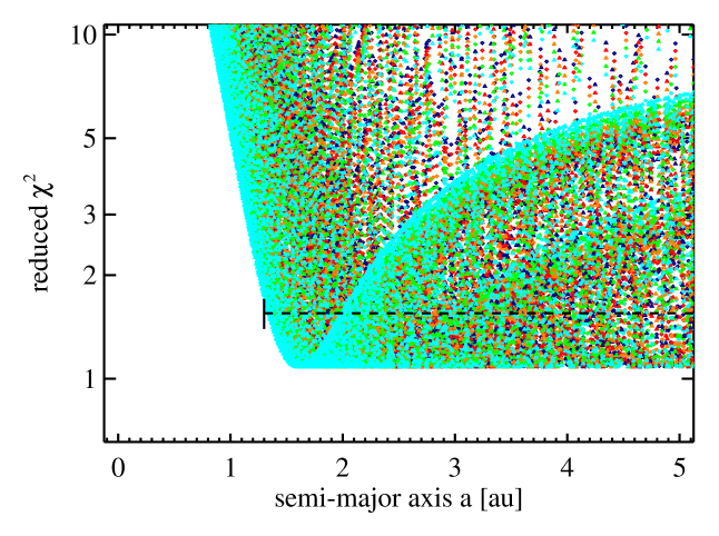
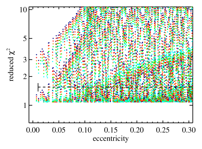
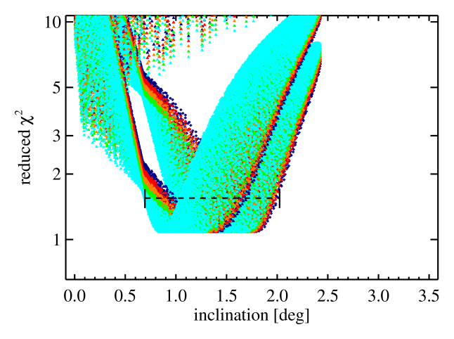
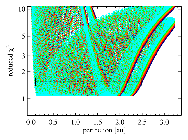
Figure 9: Orbit constraints from the $\chi^{2}$-fitting of STM predictions to the measured MIRI fluxes of the new object. From top to bottom: (i) Semi-major axis $a$; (ii) eccentricity; (iii) inclination; (iv) perihelion distance. The possible ranges are shown at reduced $\chi^{2}=1.55$ (8 degrees of freedom).

Appendix B WISE observations of MBA (10920) 1998 BC1

We extracted all available WISE measurements for (10920) from the different cryogenic and post-cryogenic data sets. The magnitudes were translated into fluxes and color-corrected to obtain monochromatic flux densities at the WISE reference wavelengths. The error calculation is described above. We excluded the WISE W1 band as it is dominated by reflected sunlight for this outer main-belt object.

Table 4: Extracted WISE fluxes for the main-belt asteroid (10920).

JDa	$\lambda$ [$\mu$m]b	flux [mJy]c	error [mJy]d	r [au]e	$\Delta$ [au]f	$\alpha$ [∘]g	Bandh	Commentsi
2455211.99146	11.10	56.043	4.070	3.0453	2.8596	18.8	W3	A,QFr10
2455212.12390	11.10	53.471	3.870	3.0455	2.8579	18.8	W3	A,QFr10
2455212.25620	11.10	26.947	2.010	3.0457	2.8562	18.8	W3	A,QFr10
2455212.38851	11.10	50.877	3.682	3.0459	2.8545	18.8	W3	A,QFr10
2455212.45472	11.10	29.959	2.226	3.0460	2.8536	18.8	W3	A,QFr10
2455212.52081	11.10	59.940	4.354	3.0461	2.8528	18.8	W3	A,QFr10
2455212.52094	11.10	58.307	4.207	3.0461	2.8528	18.8	W3	A,QFr10
2455212.58703	11.10	46.915	3.407	3.0462	2.8519	18.8	W3	A,QFr10
2455212.71933	11.10	62.190	4.473	3.0464	2.8502	18.8	W3	A,QFr10
2455212.85176	11.10	36.385	2.652	3.0466	2.8485	18.8	W3	A,SAASEP=-3 QFr10
2455212.98407	11.10	39.493	2.878	3.0468	2.8468	18.8	W3	A,QFr10
2455379.80106	11.10	32.071	2.373	3.2857	3.0205	-17.9	W3	A,QFr10
2455379.93336	11.10	39.095	2.859	3.2859	3.0225	-17.9	W3	A,QFr10
2455380.06566	11.10	23.644	1.779	3.2860	3.0245	-17.9	W3	A,QFr10
2455380.19797	11.10	26.749	2.013	3.2862	3.0266	-17.9	W3	A,QFr10
2455380.26406	11.10	23.973	1.796	3.2863	3.0276	-17.9	W3	A,SAASEP=+10 QFr10
2455380.33014	11.10	39.932	2.910	3.2864	3.0286	-17.9	W3	A,SAASEP=+2 QFr10
2455380.33027	11.10	39.059	2.878	3.2864	3.0286	-17.9	W3	A,SAASEP=+3 QFr10
2455380.46245	11.10	22.936	1.726	3.2866	3.0306	-17.9	W3	A,QFr10
2455380.46257	11.10	25.057	1.861	3.2866	3.0306	-17.9	W3	A,QFr10
2455380.52866	11.10	37.646	2.754	3.2867	3.0316	-17.9	W3	A,QFr10
2455380.59475	11.10	20.518	1.573	3.2868	3.0326	-17.9	W3	A,QFr10
2455380.66097	11.10	25.782	1.915	3.2868	3.0336	-17.9	W3	A,QFr10
2455380.79327	11.10	19.112	1.459	3.2870	3.0357	-17.9	W3	A,QFr10
2455380.92557	11.10	35.952	2.660	3.2872	3.0377	-17.9	W3	A,QFr10
2455381.05788	11.10	30.153	2.259	3.2874	3.0397	-17.9	W3	A,QFr10
2455211.99146	22.64	163.410	12.593	3.0453	2.8596	18.8	W4	A,QFr10
2455212.12390	22.64	164.770	12.698	3.0455	2.8579	18.8	W4	A,QFr10
2455212.25620	22.64	92.572	7.245	3.0457	2.8562	18.8	W4	A,QFr10
2455212.38851	22.64	149.307	11.450	3.0459	2.8545	18.8	W4	A,QFr10
2455212.45472	22.64	96.579	8.613	3.0460	2.8536	18.8	W4	A,QFr10
2455212.52081	22.64	166.755	12.494	3.0461	2.8528	18.8	W4	A,QFr10
2455212.52094	22.64	184.536	14.759	3.0461	2.8528	18.8	W4	A,QFr10
2455212.58703	22.64	140.243	11.216	3.0462	2.8519	18.8	W4	A,QFr10
2455212.71933	22.64	178.024	13.789	3.0464	2.8502	18.8	W4	A,QFr10
2455212.85176	22.64	114.942	9.809	3.0466	2.8485	18.8	W4	A,SAASEP=-3 QFr10
2455212.98407	22.64	122.484	10.022	3.0468	2.8468	18.8	W4	A,QFr10
2455379.80106	22.64	122.710	9.869	3.2857	3.0205	-17.9	W4	A,QFr10
2455379.93336	22.64	123.617	9.434	3.2859	3.0225	-17.9	W4	A,QFr10
2455380.06566	22.64	82.886	6.782	3.2860	3.0245	-17.9	W4	A,QFr10
2455380.19797	22.64	96.135	8.359	3.2862	3.0266	-17.9	W4	A,QFr10
2455380.26406	22.64	78.719	7.204	3.2863	3.0276	-17.9	W4	A,SAASEP=+10 QFr10
2455380.33014	22.64	122.710	9.760	3.2864	3.0286	-17.9	W4	A,SAASEP=+2 QFr10
2455380.33027	22.64	126.148	10.833	3.2864	3.0286	-17.9	W4	A,SAASEP=+3 QFr10
2455380.46245	22.64	80.627	7.010	3.2866	3.0306	-17.9	W4	A,QFr10
2455380.46257	22.64	75.942	6.950	3.2866	3.0306	-17.9	W4	A,QFr10
2455380.52866	22.64	131.486	9.987	3.2867	3.0316	-17.9	W4	A,QFr10
2455380.59475	22.64	75.107	6.370	3.2868	3.0326	-17.9	W4	A,QFr10
2455380.66097	22.64	79.374	7.554	3.2868	3.0336	-17.9	W4	A,QFr10
2455380.79327	22.64	67.746	6.321	3.2870	3.0357	-17.9	W4	A,QFr10
2455380.92557	22.64	128.493	10.513	3.2872	3.0377	-17.9	W4	A,QFr10
2455381.05788	22.64	102.443	8.382	3.2874	3.0397	-18.0	W4	A,QFr10
2455211.99146	4.60	0.299	0.072	3.0453	2.8596	18.8	W2	ISU,B,QFr10
2455212.45472	4.60	0.139	0.050	3.0460	2.8536	18.8	W2	ISU,B,QFr10
2455212.52081	4.60	0.146	0.052	3.0461	2.8528	18.8	W2	ISU,B,QFr10
2455212.52094	4.60	0.297	0.068	3.0461	2.8528	18.8	W2	ISU,B,QFr10
2455212.58703	4.60	0.171	0.053	3.0462	2.8519	18.8	W2	ISU,B,QFr10
2455212.71933	4.60	0.167	0.049	3.0464	2.8502	18.8	W2	ISU,B,QFr10
2455379.93336	4.60	0.277	0.063	3.2859	3.0225	-17.9	W2	ISU,B,QFr10
2455380.33027	4.60	0.221	0.063	3.2864	3.0286	-17.9	W2	ISU,B,SAASEP=+3 QFr10
2456674.91650	4.60	0.257	0.084	2.8588	2.6455	-20.1	W2	NIS,B,QFr5
2456675.04830	4.60	0.198	0.063	2.8587	2.6472	-20.1	W2	NIS,B,QFr10
2456675.31176	4.60	0.214	0.059	2.8583	2.6505	-20.1	W2	NIS,B,QFr10
2456675.31189	4.60	0.217	0.058	2.8583	2.6505	-20.1	W2	NIS,B,QFr10
2456675.64118	4.60	0.219	0.061	2.8580	2.6547	-20.1	W2	NIS,B,QFr10
2456675.90477	4.60	0.215	0.077	2.8576	2.6580	-20.1	W2	NIS,B,QFr10
2456676.03657	4.60	0.297	0.070	2.8575	2.6597	-20.1	W2	NIS,B,QFr10
2456974.42707	4.60	0.438	0.102	2.7188	2.5230	21.4	W2	NIS,B,QFr5
2456974.55848	4.60	0.449	0.106	2.7188	2.5213	21.3	W2	NIS,B,QFr10
2456974.55861	4.60	0.331	0.093	2.7188	2.5213	21.3	W2	NIS,B,QFr10
2456974.82156	4.60	0.315	0.101	2.7189	2.5179	21.3	W2	NIS,B,QFr10
2456974.95297	4.60	0.718	0.194	2.7190	2.5162	21.3	W2	NIS,B,QFr10
2456975.15022	4.60	1.671	0.361	2.7191	2.5136	21.3	W2	NIS,B,QFr10
2456977.97713	4.60	0.521	0.094	2.7202	2.4770	21.3	W2	NIS,B,QFr5
2456978.37162	4.60	0.364	0.091	2.7203	2.4719	21.3	W2	NIS,B,QFr10
2456978.50304	4.60	0.325	0.071	2.7204	2.4702	21.3	W2	NIS,B,QFr10
2456978.56874	4.60	0.327	0.075	2.7204	2.4694	21.3	W2	NIS,B,QFr10
2456978.70028	4.60	0.369	0.082	2.7205	2.4677	21.3	W2	NIS,B,QFr10
2456978.76599	4.60	0.276	0.063	2.7205	2.4668	21.3	W2	NIS,B,QFr10
2456978.83170	4.60	0.193	0.059	2.7205	2.4660	21.3	W2	NIS,B,QFr10
2456979.09465	4.60	0.391	0.095	2.7206	2.4626	21.3	W2	NIS,B,QFr5
2456979.22619	4.60	0.341	0.071	2.7207	2.4609	21.2	W2	NIS,B,QFr10
2457138.42474	4.60	0.394	0.095	2.8500	2.4988	-20.4	W2	NIS,B,QFr10
2457141.57509	4.60	0.258	0.069	2.8537	2.5436	-20.5	W2	NIS,B,QFr10
2457141.57522	4.60	0.246	0.085	2.8537	2.5436	-20.5	W2	NIS,B,QFr10
2457141.96895	4.60	0.243	0.073	2.8541	2.5492	-20.5	W2	NIS,B,QFr5
2457142.23152	4.60	0.262	0.078	2.8544	2.5530	-20.5	W2	NIS,B,QFr5
2457142.69095	4.60	0.189	0.061	2.8550	2.5596	-20.5	W2	NIS,B,QFr10
2458725.70223	4.60	0.217	0.061	2.8861	2.6835	20.5	W2	NIS,B,QFr10
2458725.96379	4.60	0.233	0.064	2.8858	2.6797	20.5	W2	NIS,B,QFr10
2458726.09469	4.60	0.224	0.076	2.8856	2.6778	20.5	W2	NIS,B,QFr10
2458726.16014	4.60	0.295	0.085	2.8855	2.6768	20.5	W2	NIS,B,QFr10
2458726.22547	4.60	0.288	0.079	2.8854	2.6759	20.5	W2	NIS,B,QFr5
2458726.42182	4.60	0.224	0.067	2.8852	2.6730	20.5	W2	NIS,B,QFr5
2458726.81428	4.60	0.226	0.075	2.8847	2.6674	20.5	W2	ISC,B,QFr5
2458726.94505	4.60	0.230	0.074	2.8845	2.6655	20.5	W2	NIS,B,QFr5
2458875.40095	4.60	0.464	0.085	2.7412	2.2133	-19.4	W2	NIS,B,QFr10
2458875.53185	4.60	0.315	0.073	2.7411	2.2149	-19.4	W2	NIS,B,QFr10
2458875.66263	4.60	0.175	0.056	2.7411	2.2164	-19.5	W2	NIS,B,QFr10
2458875.79340	4.60	0.285	0.068	2.7410	2.2180	-19.5	W2	NIS,B,QFr10
2458875.85885	4.60	0.213	0.067	2.7409	2.2187	-19.5	W2	NIS,B,QFr10
2458875.92418	4.60	0.504	0.102	2.7409	2.2195	-19.5	W2	NIS,B,QFr10
2458875.92431	4.60	0.500	0.091	2.7409	2.2195	-19.5	W2	NIS,B,QFr5
2458875.98912	4.60	0.230	0.076	2.7408	2.2203	-19.5	W2	NIS,B,QFr10
2458876.12053	4.60	0.449	0.080	2.7408	2.2219	-19.5	W2	NIS,A,QFr10
2458876.25131	4.60	0.353	0.072	2.7407	2.2234	-19.5	W2	NIS,B,QFr10
2458876.38209	4.60	0.236	0.062	2.7406	2.2250	-19.6	W2	ISC,B,QFr10
2459199.33575	4.60	0.319	0.070	2.8360	2.6434	20.3	W2	NIS,B,QFr5
2459199.46653	4.60	0.190	0.063	2.8362	2.6417	20.3	W2	NIS,B,QFr5
2459199.85886	4.60	0.311	0.079	2.8366	2.6367	20.3	W2	NIS,B,SAASEP=+0 QFr5
2459199.92418	4.60	0.220	0.065	2.8367	2.6359	20.3	W2	NIS,B,SAASEP=-6 QFr10
2459200.05445	4.60	0.265	0.076	2.8368	2.6343	20.3	W2	NIS,B,QFr10
2459200.31651	4.60	0.253	0.069	2.8371	2.6309	20.3	W2	NIS,B,QFr10
2459200.44728	4.60	0.241	0.065	2.8373	2.6293	20.3	W2	NIS,B,QFr10
2459200.57806	4.60	0.255	0.063	2.8374	2.6276	20.3	W2	NIS,B,QFr5
2459348.02845	4.60	0.172	0.049	3.0301	2.4990	-18.0	W2	NIS,B,QFr5

Table 4: continued

^a The observation epoch (Julian date); ^b the reference wavelength in the given bands (in $\mu$m); ^c the color-corrected, monochromatic flux densities at the reference wavelength (in mJy); ^d the absolute flux errors (in mJy); ^e the helio-centric distance r (in au); ^f the observer-object distance (au); ^g the phase angle (in ^∘; ^h the band name; ⁱ quality comments: all measurements were not saturated and had photometry quality flags ’A’ (SNR$\geq$10) or ’B’ (3$\leq$SNR$<$10). Cases with South-Atlantic-Anomaly (SAA) separations $\leq$10^∘ are flagged. Only quality frame (QFr) scores 5 or 10 were accepted. For W2 detections we also listed the WISE catalog comments ”NIS” (NoInertialSource), ”ISU” (InertialSourceUndecided) or ”ISC” (InertialSourceContamination).

With the current spin-shape solution it is unfortunately not possible to combine all data over 12 year as the rotation period is not known with sufficient quality. However, the high-SNR WISE W3 and W4 data from January and July 2010 can be phased very well. They show a strong rotational variation (see Fig. 10), perfectly consistent with the lightcurve-derived rotation period. These flux changes are explained by an ellipsoidal shape model with a/b $\approx$ 1.5. The dual-band data are nicely balanced before and after opposition. The radiometric study resulted in a thermal inertia of 15 J m^-2s^-0.5K^-1 which allows to unify the observation-to-model ratio for both bands and all before/after opposition data from 2010 (reduced $\chi^{2}$ close to unity). The best-fit sizes are 14.7 km for the spherical shape, and 15.3 km for the ellipsoidal model (size of an equal-volume sphere). The ellipsoidal spin-shape solution was also used for the JWST observations, with a rotational phasing directly connected to our 2022 lightcurve measurements (see Fig. 2).

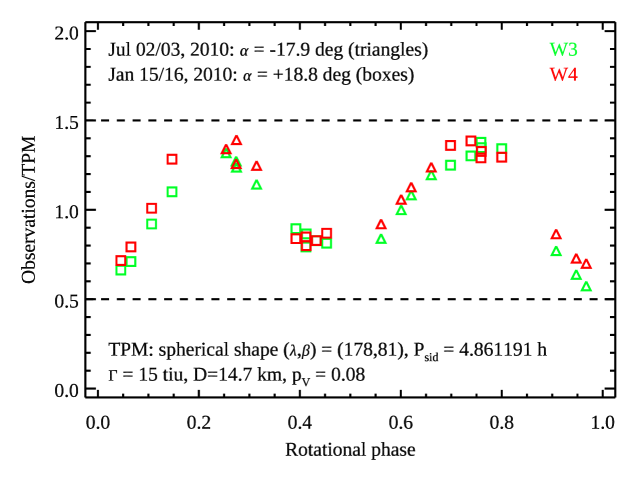
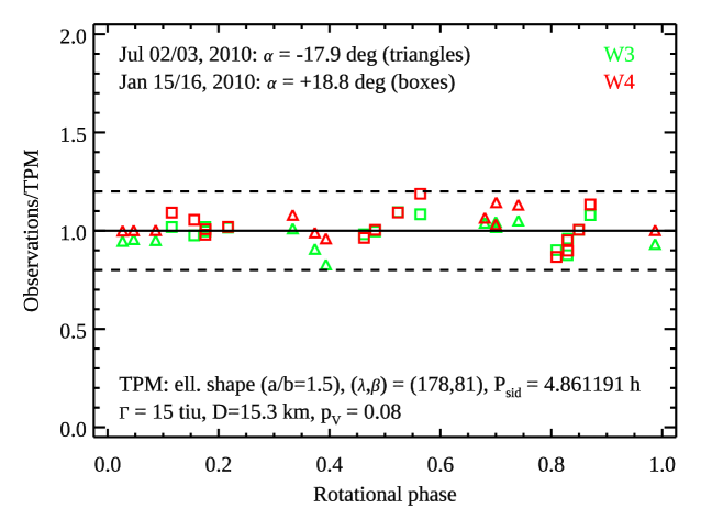
Figure 10: WISE W3 and W4 data from 2010 from both epochs before and after opposition. Left: WISE observations divided by a TPM prediction assuming a spherical shape. Right: divided by a TPM prediction assuming an ellipsoidal shape with a/b = 1.5. For both figures we take the same spin and thermal properties into account.