Regret-based Optimization for Robust Reinforcement Learning

Abstract

Deep Reinforcement Learning (DRL) policies are vulnerable to adversarial noise in observations, which can have disastrous consequences in safety-critical environments. For instance, a self-driving car receiving adversarially perturbed sensory observations about traffic signs (e.g., a stop sign physically altered to be perceived as a speed limit sign) can be fatal. Leading existing approaches for making RL algorithms robust to an observation-perturbing adversary have focused on (a) regularization approaches that make expected value objectives robust by adding adversarial loss terms; or (b) employing “maximin” (i.e., maximizing the minimum value) notions of robustness. While regularization approaches are adept at reducing the probability of successful attacks, they remain vulnerable when an attack is successful. On the other hand, maximin objectives, while robust, can be too conservative to be useful. To this end, we focus on optimizing a well-studied robustness objective, namely regret. To ensure the solutions provided are not too conservative, we optimize an approximation of regret using three different methods. We demonstrate that our methods are able to outperform existing best approaches for adversarial RL problems across a variety of standard benchmarks from literature.

1 Introduction

Harnessing the power of Deep Neural Networks in DRL (Mnih et al. 2013) allows RL models to achieve outstanding results on complex and even safety-critical tasks, such as self-driving (Spielberg et al. 2019; Kiran et al. 2021). However, DNN performance is known to be vulnerable to attacks on input, and DRL models are not exempt (Gleave et al. 2019; Sun et al. 2020; Pattanaik et al. 2017). In such perturbations, adversaries only alter the observations received by an RL agent and not the underlying state or the dynamics (transition function) of the environment. Even with limited perturbations, high-risk tasks such as self-driving yield opportunities for significant harm to property and loss of life. One such example is presented by (Chen et al. 2018), in which a stop sign is both digitally and physically altered to attack an object recognition model.

Although the viability of known adversarial examples can be mitigated by adversarial training (supervised training against adversarial examples) (Gleave et al. 2019; Goodfellow, Shlens, and Szegedy 2014; Pattanaik et al. 2017; Sun et al. 2023), this does not guarantee the ability to generalize to unseen adversaries. Additionally, it has been shown that naive adversarial training in RL leads to unstable training and lowered agent performance, if effective at all (Zhang et al. 2020). Thus, we need algorithms that are not tailored to specific adversarial perturbations but are inherently robust. The intuition is, rather than develop a policy that is value-optimal for as many known examples as possible, we want to determine what behavior and states involve risk and reduce them across the horizon. To achieve this, maximin methods operate to maximize the minimum reward of a policy (Everett, Lütjens, and How 2020; Liang et al. 2022), which can be robust but oftentimes trades unperturbed solution quality to fortify the lower bound. Regularization methods construct adversarial loss terms to ensure actions remain unchanged across similar inputs (Oikarinen et al. 2021; Zhang et al. 2020; Liang et al. 2022), reducing the probability of a successful adversarial attack. However, as we empirically show later, they remain vulnerable when attacks are successful.

To these ends, we provide a regret-based adversarial defense approach that aims to reduce the impact of a successful attack without being overly conservative.

Contributions: We make the following key contributions:

• Formally define regret in settings where an observation-perturbing adversary is present. Regret is defined as the difference in value achieved in the absence and in the presence of an observation-perturbing adversary.

• Derive an approximation of regret, named Cumulative Contradictory Expected Regret (CCER), which is amenable to scalable optimization due to satisfying the optimal sub-structure property. We provide a value iteration approach to minimize CCER, named RAD-DRN (Regret-based Adversarial Defense with Deep Regret Networks). Our approach can balance the robustness of solutions obtained using CCER with maximizing solution quality;

• We provide a policy gradient approach to minimize CCER, named RAD-PPO. We derive the policy gradient w.r.t the regret measure and utilize it in the PPO framework.

• To demonstrate the applicability of regret even to reactive approaches, we provide a Cognitive Hierarchy Theory (CHT) based approach that generates potential adversarial policies and computes a regret-based robust response. We refer to this approach as RAD-CHT.

• Finally, we provide detailed experimental results on multiple benchmark problems (MuJoCo, Atari, and Highway) to demonstrate the utility of our approaches against several leading approaches in adversarial RL. More importantly, we demonstrate the performance of our approach against not only strong myopic attacks (e.g., PGD) but also multi-step attacks that are computed based on knowledge of the computed victim policy.

2 Related Work

Adversarial Attacks in RL. Deep RL has shown to be vulnerable to attacks on its input, whether from methods with storied success against DNNs such as an FGSM attack (Huang et al. 2017; Goodfellow, Shlens, and Szegedy 2014), tailored attacks against the value function (Kos and Song 2017; Sun et al. 2020), or adversarial behavior learned by an opposing policy (Gleave et al. 2019; Everett, Lütjens, and How 2020; Oikarinen et al. 2021; Zhang et al. 2020). We compile attacks on RL loosely into two groups of learned adversarial policies: observation poisonings (Gleave et al. 2019; Sun et al. 2020; Lin et al. 2017) and direct ego-state disruptions (Pinto et al. 2017; Rajeswaran et al. 2017). Each category has white-box counterparts that leverage the victim’s network gradients to generate attacks (Goodfellow, Shlens, and Szegedy 2014; Oikarinen et al. 2021; Huang et al. 2017; Everett, Lütjens, and How 2020). While previous methods focus on robustness against one or the other, we demonstrate that the proposed methods are comparably robust to both categories of attacks.

Adversarial Training. In this area, adversarial examples are found or generated and integrated into the set of training inputs (Shafahi et al. 2019; Ganin et al. 2016; Wong, Rice, and Kolter 2020; Madry et al. 2017; Andriushchenko and Flammarion 2020; Shafahi et al. 2020). For a comprehensive review, we refer readers to (Bai et al. 2021). In RL, research efforts have demonstrated the viability of training RL agents against adversarial examples (Gleave et al. 2019; Bai, Guan, and Wang 2019; Pinto et al. 2017; Tan et al. 2020; Kamalaruban et al. 2020). Naively training RL agents against known adversaries is a sufficient defense against known attacks; however, new or more general adversaries remain effective (Gleave et al. 2019; Kang et al. 2019) and therefore we focus on proactively robust defense methods instead of reactive (react to known adversaries) defense methods.

Robustness through Regularization. Regularization approaches (Zhang et al. 2020; Oikarinen et al. 2021; Everett, Lütjens, and How 2020) consider networks that are trained using a combination of the expected value loss function and loss due to adversarial perturbations. These approaches utilize certifiable robustness bounds computed for neural networks when evaluating adversarial loss and ensure the probability of success of an attack is reduced using these lower bounds. Despite lowering the likelihood of a successful attack, an attack that does break through will still be effective (as shown in Table 1). Note that for RADIAL (a regularization approach), even though the success percentage of attacks is the least, it has the largest drop in performance.

Algo.	Num. Atks	% Success	Score
RADIAL	6	5%	4.16
WoCaR	6	12%	6.63
RAD-DRN	6	40%	9.9
RAD-PPO	7	10%	18
RAD-CHT	8	60%	20.1

Table 1: The impact and frequency of successful attacks on an example set of the Strategically Timed Attack (Lin et al. 2017) on highway-fast-v0, where the unperturbed score is $\!\!>\!\!22$ for all methods. The Num. Atks column shows the number of attempted attacks; the % Success column indicates the rate at which an attempted attack changed the selected action.

Regret Optimization in MDPs. Measuring and optimizing a regret value to improve the robustness has been studied previously in uncertain MDPs(Ahmed et al. 2013; Rigter, Lacerda, and Hawes 2021). In RL, (Jin, Keutzer, and Levine 2018) established Advantage-Like Regret Minimization (ARM) as a policy gradient solution for agents robust to partially-observable environments. While the properties and optimization of regret are in general well-studied, current applications in RL focus on utilizing regret as a robustness tool against natural environment variance; to the best of our knowledge, this is the first application of regret to defend against strategic adversarial perturbations.

3 RL with Adversarial Observations

In problems of interest, we have an RL agent whose state/observation and action space are $S$ and $A$ respectively. There is an underlying transition function $T:S\times A\times S\rightarrow[0,1]$ and reward model $R:S\times A\rightarrow\mathbb{R}$ which are not known a priori to the RL agent. The behavior of the agent is governed by a policy $\pi:S\rightarrow A$ that maps states to actions. The typical objective for an RL agent is to learn a policy ${\pi}^{*}$ that maximizes its expected value without knowing the underlying transition and reward model a priori. This can be formulated as the following optimization problem:

$${\pi}^{*}\in\arg\max\nolimits_{{\pi}}V^{\pi}(s_{0})$$

where $V^{\pi}(s_{0})$ is the expected accumulated value the RL agent obtains starting from state $s_{0}$ for executing policy $\pi$. The policy computed is not robust in the presence of an adversary who can strategically alter the observation received by the agent at any time step. This is because the agent could be executing the wrong action for the underlying state.

For the rest of this paper, we will use $z_{t}$ to represent the observed (possibly perturbed) state and $s_{t}$ to refer to the true underlying state at step $t$. Formally, on taking action $a_{t}$ in state $s_{t}$, the environment transitions to a new state $s_{t+1}$. However, the adversary can alter the observation received by the RL agent to another state $z_{t+1}$ instead of $s_{t+1}$ to reduce the expected value of the RL agent, where $z_{t+1}\in N(s_{t+1})$ — a set of neighbors of $s_{t+1}$, defined as follows:

$$N(s_{t})=\{z_{t}:\|{z}_{t}-s_{t}\|_{\infty}\leq\epsilon\}$$

Often, it is not possible for the agent to recognize if the observation is perturbed or not. For example, given a highway speed limit sign, an adversary perturbing the sign to provide a different speed limit may be indistinguishable for an agent and hence would be within the neighborhood. However, this is within a reasonable constraint; perturbing the speed limit sign to be a stop sign may be easy to heuristically distinguish and hence would not be part of the neighborhood.

We now can represent the observation-altering adversarial policy as $\mu:S\rightarrow S$. The notion of neighborhoods translates to adversarial policies $\mu$ such that $\mu(s)\in N(s)$. When the adversarial policy is deterministic and bijective, for a given observed state ${z}$, we will employ $\mu^{-1}({z})$ to retrieve the underlying unperturbed state $s\in N(z)$. In the following, we focus on computing policies that are inherently robust, even without knowing the adversary policy.

4 Regret-based Adversarial Defense (RAD)

Our approach to computing inherently robust policies is based on minimizing the maximum regret the agent receives for taking the wrong action assuming there was a perturbation in states. We first introduce the notions of regret and max regret for the RL agent to play a certain policy $\pi$. The regret-based robust policy is then formulated accordingly.

Definition 1 (Regret).

Given an adversary policy $\mu$, the regret at each observed state $z_{t}$ for the RL agent to play a policy $\pi$ is defined as follows:

$$\delta^{\pi,\mu}(z_{t})=V^{\pi}(z_{t})-V^{\pi,\mu}(z_{t})$$ (1)

Intuitively, it is the difference between the expected value $V^{\pi}(\cdot)$ (assuming no adversary) and the value $V^{\pi,\mu}(\cdot)$ (assuming states are being perturbed by the adversary policy $\mu$) while the RL agent takes actions according to a policy $\pi$. In particular, the value for an agent with a policy $\pi$ in the absence of an adversary, $V^{\pi}(\cdot)$, is given by:

$$V^{\pi}(z_{t}) =R(z_{t},\pi(z_{t}))+\gamma\mathbb{E}_{z_{t+1}}\big{[}V^{\pi}(z_{t+1})\big{]}$$ (2)

where $z_{t+1}\sim T(\cdot|z_{t},\pi(z_{t}))$. Note that when the adversary is not present, the observed states $z_{t}=s_{t}$ and $z_{t+1}=s_{t+1}$.

On the other hand, the $V^{\pi,\mu}(.)$ function for an agent with policy $\pi$ in the presence of such an adversary $\mu$ is given by:

$$V^{\pi,\mu}(z_{t}) \!=\!R(s_{t},\pi(z_{t}))\!+\!\gamma\mathbb{E}_{z_{t+1}}\big{[}V^{\pi,\mu}({z}_{t+1})\big{]}$$ (3)

where $s_{t}\!\!=\!\!\mu^{-1}\!(z_{t})$, $z_{t+1}\!\!=\!\!\mu(s_{t+1})$ with $s_{t+1}\!\!\sim\!\!T(\cdot|s_{t},\pi(z_{t}))$. Note that our regret is defined based on observed states, as the agent will only have access to observed states (and not the true states) when making test-time decisions.

Definition 2 (Minimax Regret Policy).

The regret-based robust policy for the RL agent is the policy that minimizes the maximum regret at the initial observed state $z_{0}$ over all possible adversary policies, formulated as follows:

$${\pi}^{*}\in\arg\min\nolimits_{{\pi}}\;\max\nolimits_{\mu}\;\delta^{\pi,\mu}(z_{0})$$ (4)

Intuitively, a minimax regret policy minimizes the maximum regret by avoiding the actions which have high variance across neighboring states. Unfortunately, there are multiple issues with optimizing minimax regret. First, optimizing regret requires iterating over different adversary policies, which can be infinite depending on the state and action spaces. If we assume specific types of adversaries, robustness may not extrapolate to other adversary policies. Second, the minimax regret expression does not exhibit optimal substructure property, thus rendering value iteration approaches (e.g., Q-learning, DQN) theoretically invalid. Third, deriving policy gradients w.r.t. regret is computationally challenging, requiring combinatorial perturbed trajectory simulations. As a result, employing policy gradient approaches to optimize regret is also infeasible.

We address the above issues by using an approximate notion of regret referred to as Cumulative Contradictory Expected Regret (CCER) and then proposing two types of approaches (adversary agnostic and adversary dependent):

• Adversary agnostic approach for optimizing approximate regret: CCER has multiple useful properties: (i) It satisfies the optimal substructure property, thereby allowing for usage of a DQN type approach; and (ii) It is possible to compute a policy gradient with regards to CCER, thereby allowing for a policy gradient approach.

• Adversary dependent approach for optimizing approximate regret: We utilize an iterative best-response approach based on Cognitive Hierarchical Theory (CHT) to ensure defense against a distribution of “good” adversarial policies. This approach is referred to as RAD-CHT.

4.1 Regret Approximation: CCER

We introduce a new notion of approximate regret, referred to as CCER. CCER accumulates contradictory regret at each epoch; we refer to this regret as contradictory as the observed state’s optimal action may contradict the true state’s action. The key intuition is that we accumulate the regret (maximum difference in reward) in each time step regardless of whether the state is perturbed or not perturbed.

For the underlying transition function, $T$, and reward model, $R$, CCER w.r.t a policy $\pi$ is defined as follows:

$$\delta_{\texttt{CCER}}^{\pi}(z_{t}) =R(z_{t},\pi(z_{t}))-\min\nolimits_{s_{t}\in N({z_{t}})}R(s_{t},\pi(z_{t}))$$

$$\hskip 28.90755pt+\gamma\mathbb{E}_{z_{t+1}}\Big{[}\delta_{\texttt{CCER}}^{\pi}(z_{t+1})\Big{]}$$ (5)

where $z_{t+1}\sim T(\cdot|z_{t},\pi(z_{t}))$. Our goal is to compute a policy that minimizes CCER, i.e.,

$$\pi^{\bot}\in\arg\min\nolimits_{\pi}\;\delta_{\texttt{CCER}}^{\pi}(z_{0})$$

This is a useful objective, as CCER accumulates the myopic regrets at each time step and we minimize this overall accumulation. Importantly, CCER has the optimal substructure property, i.e., the optimal solution for a sub-problem (from step $t$ to horizon $H$) is also part of the optimal solution for the overall problem (from step $0$ to horizon $H$).

Proposition 1 (Optimal Substructure property).

At time step $t$, the CCER corresponding to a policy, $\pi$ at $z_{t}$, i.e., $\delta_{\texttt{CCER}}^{\pi}(z_{t})$ is minimum if it includes the CCER minimizing policy from $t+1$, i.e.,$\pi^{\bot}_{[t+1,H]}$ from $t+1$. Formally,

$$\delta_{\texttt{CCER}}^{\left<\pi_{t},\pi^{\bot}_{[t+1,H]}\right>}(z_{t})\leq\delta_{\texttt{CCER}}^{\left<\pi_{t},\pi_{[t+1,H]}\right>}(z_{t})$$

All proofs are in Appendix A. Similar to the state and state-action value function, $V(s)$ and $Q(s,a)$, we also have state regret, $\delta^{\pi}_{\texttt{CCER}}(z_{t})$ and state-action regret, $\delta^{\pi}_{\texttt{CCER}}(z_{t},a_{t})$. Specific definitions are provided in the following sections.

4.2 Approach 1: RAD-DRN

We first provide a mechanism similar to DQN (Mnih et al. 2015) to compute a robust policy that minimizes CCER irrespective of any adversary. Briefly, we accumulate the regret over time steps (rather than reward) and act on the minimum of this estimate (rather than the maximum, as a DQN would). Intuitively, minimizing CCER ensures the obtained policy avoids taking actions that have high variance, therefore avoiding volatile states which have high regret. In our adversarial setting, this roughly corresponds to behavior that avoids states where false observations have q-values vastly different from the underlying state. In a driving scenario, for example, this could mean giving vehicles and obstacles enough berth to account for errors in distance sensing. Let us denote by:

$$\delta^{\pi}_{\texttt{CCER}}(z,a) =R(z,a)-\min\nolimits_{s\in N(z)}R(s,a)$$

$$\qquad\qquad+\gamma\mathbb{E}_{z^{\prime}}\left[\min\nolimits_{a^{\prime}}\delta^{\pi}_{\texttt{CCER}}(z^{\prime},a^{\prime})\right]$$

as the q-value associated with CCER in our setting. We provide the pseudocode of our algorithm, named RAD-DRN, employing a neural network to predict $\delta_{\texttt{CCER}}(z,a)$ in Alg. 1. This network’s parameter $w$ is trained based on minimizing the loss between the predicted and observed $\delta_{\texttt{CCER}}$ values.

1 Initialize replay memory $D$ to capacity $N$;

2 Initialize q-regret $\delta_{\texttt{CCER}}$ with random weights $w$;

3 Initialize target q-regret $\widehat{\delta}_{\texttt{CCER}}$ with weights $w^{-}=w$;

4 for $\text{episode}=1\to M$ do

5       Get initial state $z_{0}$;

6       for $t=0\to H$ do

7             With prob. $\epsilon$, select a random action $a_{t}$;

8             Else, select $a_{t}\in\operatorname*{argmin}_{a}\delta_{\texttt{CCER}}(z_{t},a,w)$;

9             Execute action $a_{t}$, get observed state $z_{t+1}$;

10             Observe regret $r_{t}\!=\!R(z_{t},a_{t})\!-\!\!\!\!\min\limits_{s_{t}\in N(z_{t})}\!\!\!\!R(s_{t},a)$;

11             Store transition $(z_{t},a_{t},z_{t+1},r_{t})\rightarrow D$;

12             Sample mini-batch $(z_{i},a_{i},z_{i+1},r_{i})\sim D$;

13             for each $(z_{i},a_{i},z_{i+1},r_{i})$ in mini-batch do

14                   $\text{Set target }y_{i}=\begin{cases}r_{i}\text{, if episode terminates at step $i+1$}\\ r_{i}+\gamma\min_{a^{\prime}}\widehat{\delta}_{\texttt{CCER}}(z_{i+1},a^{\prime};w^{-})\text{, otherwise }\end{cases}$

15                   Perform a gradient descent to update $w$ based on loss: $\big{[}y_{i}-\delta_{\texttt{CCER}}\big{(}z_{i},a_{i},w\big{)}\big{]}^{2}$;

16                  

17            

18      Every $K$ steps reset $w^{-}=w$;

Algorithm 1 RAD-DRN

Given the conservative nature of regret, RAD-DRN can provide degraded nominal (unperturbed) performance, especially in settings with very few high-variance states. We propose a heuristic optimization trick to reduce unnecessary conservatism in RAD-DRN. We consider using weighted combinations of value and CCER estimates to determine the utility of employing each policy at a given observation. Intuitively, we want to apply a value-maximizing policy in low-variance state neighborhoods and a regret-minimizing policy in high-variance neighborhoods; as such, the utility of using a regret-minimizing policy in a high-regret neighborhood will, in turn, be high. Specifically, we train a DQN to maximize the utility function:

$$Util(z,\pi)=V^{\pi}(z)-\beta\delta^{\pi}_{\texttt{CCER}}(z)$$

where $\beta$ is a caution-weight constant decimal. This final step requires a minimal amount of training ($500$ episodes) and interacts directly with the non-adversarial environment. We constrain the available actions of the utility-maximizing policy to either be the value-optimal action $\operatorname*{argmax}_{a}Q^{\pi}(z,a)$ or the CCER-optimal action $\operatorname*{argmin}_{a}\delta^{\pi}_{\texttt{CCER}}(z,a)$, avoiding actions that are sub-optimal to both measures. These two optimal DQN and RAD-DRN policies are obtained in advance before training the above utility-maximizing policy.

4.3 Approach 2: RAD-PPO

In this section, we provide a policy gradient approach that minimizes CCER. Proximal Policy Optimization (PPO), and any policy gradient (PG) method, can be extended with contradictory regret. The key contribution is defining/deriving the policy gradient based on the long-term CCER of a policy:

$$\delta_{\texttt{CCER}}^{\pi}(z)= \sum\nolimits_{a}\pi(z,a)\delta_{\texttt{CCER}}^{\pi}(z,a)$$

Proposition 2.

The gradient of a CCER-minimizing policy $\pi_{\theta}$ parameterized by $\theta$ can be computed as follows:

$$\frac{\partial\delta_{\texttt{CCER}}^{\pi_{\theta}}(z)}{\partial\theta} \!=\!\sum\nolimits_{s}\!\!P(z|\pi_{\theta})\!\sum\nolimits_{a}\!\!\frac{\partial\pi_{\theta}(z,a)}{\partial\theta}\delta_{\texttt{CCER}}^{\pi_{\theta}}(z,a)$$ (6)

where $P(z|\pi_{\theta})$ is the stationary distribution w.r.t $\pi_{\theta}$.

This can also be rewritten along similar lines as the traditional policy gradient using an expectation (instead of $P(z|\pi_{\theta})$):

$$\nabla_{\theta}\delta_{\texttt{CCER}}^{\pi_{\theta}}(z_{0})=\mathbb{E}_{\pi_{\theta}}\Big{[}\delta_{\texttt{CCER}}^{\pi_{\theta}}(z,a)\nabla_{\theta}\log\pi_{\theta}(a\mid z)\Big{]}$$

CCER-based Advantage.

Furthermore, we can replace $\delta_{\texttt{CCER}}^{\pi_{\theta}}(z,a)$ on the right side of the gradient with a CCER advantage function defined as follows:

$${A}^{\texttt{CCER}}(z_{t},a) =-[\delta_{\texttt{CCER}}^{\pi_{\theta}}(z_{t},a)-\delta_{\texttt{CCER}}^{\pi_{\theta}}(z_{t})]$$ (7)

The positive value of $|{A}^{\texttt{CCER}}|$ can be understood as the increase in regret associated with increasing $\pi_{\theta}(a|z_{t})$, as the value of the selected action relative to others will be lower when a perturbation occurs. Thus, we invert the sign so that regret and ${A}^{\texttt{CCER}}$ are inversely related, i.e. selecting the action with the highest ${A}^{\texttt{CCER}}$ will minimize regret.

4.4 Approach 3: RAD-CHT

The previous RAD-DRN and RAD-PPO approaches are agnostic to specific adversarial policies. In this section, we provide a reactive approach that identifies strong adversarial policies and computes a best-response (minimum CCER) policy against them. This approach builds on the well-known behavior model in game theory and economics referred to as Cognitive Hierarchical Theory (CHT) (Camerer, Ho, and Chong 2004). In CHT, players’ strategic reasoning is organized into multiple levels; players at each level assume others are playing at a lower level (i.e., are less strategic).

Our approach, named RAD-CHT, is an iterative algorithm that proceeds as follows:

• Iteration 0 (Level $0$): Both the RL agent and the adversary play completely at random, with the random policies for agent and adversary given by $\pi^{(0)}$ and $\mu^{(0)}$ respectively.

• Iteration 1 (Level $1$): The RL agent assumes a level $0$ adversary and wants to find a new policy $\pi^{(1)}$ that minimizes the regret given $\mu^{(0)}$, formulated as follows:

  $$\pi^{(1)} =\arg\min\nolimits_{\pi}\delta^{\pi,\mu^{[(0)]}}_{\texttt{CCER}}(z_{0})$$

  $$\delta_{\texttt{CCER}}^{\pi,\mu^{[(0)]}}(z_{t}) =R(z_{t},\pi(z_{t}))-R(s_{t},\pi(z_{t}))$$

  $$\hskip 36.135pt+\gamma\mathbb{E}_{z_{t+1}}\left[\delta_{\texttt{CCER}}^{\pi,\mu^{[(0)]}}(z_{t+1})\right]$$

  where $s_{t}$ is the true state given the observed state is $z_{t}$ and the attack policy is $\mu^{(0)}$, i.e., $\mu^{(0)}(s_{t})=z_{t}$. On the other hand, the level-$1$ adversary assumes the RL agent is at level $0$ and attempts to find a perturbation policy that minimizes the agent’s expected return:

  $$\mu^{(1)}\in\arg\min\nolimits_{\mu}V^{\pi^{(0)},\mu}(\cdot)$$

• Iteration $k>1$ (Level $k$): The agent assumes the adversary can be at any level below $k$. Like in CHT, the adversary policy is assumed to be drawn from a Poisson distribution over the levels $0,1,\cdots,k-1$ with a mean $k-1$. The RL agent then finds a new policy $\pi^{(k)}$ that minimizes the regret formulated as the following:

  $$\pi^{(k)} \in\arg\min\nolimits_{\pi}\delta^{\pi,\mu^{[(k-1)]}}_{\texttt{CCER}}(z_{0})$$

  $$\delta^{\pi,\mu^{[(k-1)]}}_{\texttt{CCER}}(z_{t}) =R(z_{t},\pi(z_{t}))-\!\!\sum\nolimits_{i=0}^{k-1}\!P^{(k)}\!(i)R(s_{t}^{(i)}\!,\pi(z_{t}))$$

  $$\qquad\qquad+\gamma\mathbb{E}_{z_{t+1}}\left[\delta_{\texttt{CCER}}^{\pi,\mu^{[(k-1)]}}(z_{t+1})\right]$$

  where $P^{(k)}(i)\propto\frac{\lambda^{i}e^{-\lambda}}{i!}$ (aka. Poisson distribution) is the probability the adversary is at level $i$ with $0\leq i\leq k-1$. The notation $[(k-1)]$ represents the range $(0),\ldots,(k-1)$. In addition, the true state is $s_{t}^{(i)}$, the observed state is $z_{t}$ and the attack policy is $\mu^{(i)}$, i.e., $\mu^{(i)}(s_{t}^{(i)})=z_{t}$.

  Similarly, the adversary at this level assumes the RL agent is at a level below $k$, following the Poisson distribution. The adversary then optimizes the perturbation policy as follows:

  $$\mu^{(k)}\in\operatorname*{argmin}\nolimits_{\mu}\sum\nolimits_{i=0}^{k-1}P^{(k)}(i)V^{\pi^{(i)},\mu}(\cdot)$$

At each iteration, the CCER minimization problem given the adversary distribution exhibits optimal substructure. Therefore, we can adapt Approach 1 and 2 to compute the CCER-minimizing policy given the adversarial distribution.

On the adversary side, we provide the policy gradient given agent policies at previous levels. Let’s denote

$$V_{\mu_{\theta}}(\cdot)=\sum\nolimits_{i=0}^{k-1}P^{(k)}(i)V^{\pi^{(i)},\mu_{\theta}}(\cdot)$$

where $\theta$ is the parameter of the adversary policy $\mu$.

Proposition 3.

The gradient of objective function of the adversary $V_{\mu_{\theta}}(\cdot)$ w.r.t $\theta$ can be computed as follows:

$$\nabla_{\theta}V_{\mu_{\theta}}\!=\!\mathbb{E}_{i\sim P^{(k)}(i),\tau\sim(\mu_{\theta},\pi^{(i)},T)}\Big{[}R(\tau)\!\sum\nolimits_{t}\!\!\nabla_{\theta}\log\mu_{\theta}(z_{t}|s_{t})\Big{]}$$

where $\tau=(s_{0},z_{0},a_{0},s_{1},z_{1},a_{1},\cdots)$ with $z_{t}\sim\mu_{\theta}(s_{t})$ is the perturbed state created by the adversary policy $\mu_{\theta}$. In addition, the reward of a trajectory $\tau$ is defined as follows:

$$R(\tau)=\sum\nolimits_{t}\gamma^{t}R(s_{t},a_{t})$$

Based on Proposition 3, finding an optimal adversarial policy at each level can be handled by a standard policy optimization algorithm such as PPO.

5 Experiments

We provide empirical evidence to answer key questions:

• How do RAD approaches (RAD-DRN, RAD-PPO, RAD-CHT) compare against leading methods for Adversarially Robust RL on well-known baselines from MuJoCo, Atari, and Highway libraries?

• For multi-step strategic attacks, how do RAD methods compare to leading defenses?

• Does RAD mitigate the value/robustness trade-off present in maximin methods?

• How does the performance of our approaches degrade as the intensity of attacks (i.e., # of attacks) is increased?

5.1 Experimental Setup

We evaluate our proposed methods on the commonly used Atari and MuJoCo domains (Bellemare et al. 2013; Todorov, Erez, and Tassa 2012), and a suite of discrete-action self-driving tasks (Leurent 2018). For the driving environments, each observation feature of the agent corresponds to the kinematic properties (coordinates, velocities, and angular bearings) of the ego-vehicle and nearby vehicles. The task for each environment is to maximize the time spent in the fast lane while avoiding collisions. The road configurations for the highway-fast-v0, merge-v0, roundabout-v0, and intersection-v0 tasks are, in order: a straight multi-lane highway, a two-lane highway with a merging on-ramp, a multi-lane roundabout, and a two-lane intersection. We use a standard training setup seen in (Oikarinen et al. 2021; Liang et al. 2022), details in Appendix C.

We compare RAD-DRN, RAD-PPO, and RAD-CHT to the following baselines: vanilla DQN (Mnih et al. 2013) and PPO (Schulman et al. 2017); a simple but robust minimax method, CARRL (Everett, Lütjens, and How 2020); a leading regularization approach, RADIAL (Oikarinen et al. 2021); and the current SOTA defense, WoCaR (Liang et al. 2022). We test all methods against both trained policy adversaries and gradient attacks, as well as the Strategically-Timed attack and Critical-Point attack, two leading multi-step strategic attacks (Lin et al. 2017; Sun et al. 2020). For RADIAL and WoCaR, we use the best-performing methods for each environment (their proposed DQNs for discrete actions, and PPOs for MuJoCo).

Table 2: Results on Highway. Each row shows the mean scores of each RL method against different attacks.

Algorithm	Unperturbed	WC Policy	PGD, $\epsilon\!\!=\!\frac{3}{255}$
highway-fast-v0
DQN	24.91$\pm$20.27	3.68$\pm$35.41	15.71$\pm$13
PPO	22.8$\pm$5.42	13.63$\pm$19.85	15.21$\pm$16.1
CARRL	24.4$\pm$1.10	4.86$\pm$15.4	12.43$\pm$3.4
RADIAL	28.55$\pm$0.01	2.42$\pm$1.3	14.97$\pm$3.1
WoCaR	21.49$\pm$0.01	6.15$\pm$0.3	6.19$\pm$0.4
RAD-DRN	24.85$\pm$0.01	22.65$\pm$0.02	18.8$\pm$24.6
RAD-PPO	21.01$\pm$1.23	20.59$\pm$4.10	20.02$\pm$0.01
RAD-CHT	21.83 $\pm$ 0.35	21.1 $\pm$ 0.24	21.48 $\pm$ 1.8
merge-v0
DQN	14.83$\pm$0.0	6.97$\pm$0.03	10.82$\pm$2.85
PPO	11.08$\pm$0.01	10.2$\pm$0.02	10.42$\pm$0.95
CARRL	12.6$\pm$0.01	12.6$\pm$0.01	12.02$\pm$0.01
RADIAL	14.86$\pm$0.01	11.29$\pm$0.01	11.04$\pm$0.91
WoCaR	14.91$\pm$0.04	12.01$\pm$0.28	11.71$\pm$0.21
RAD-DRN	14.86$\pm$0.01	13.23$\pm$0.01	11.77$\pm$1.07
RAD-PPO	13.91$\pm$0.01	13.90$\pm$0.01	11.72$\pm$0.01
RAD-CHT	14.7 $\pm$ 0.01	14.7 $\pm$ 0.12	13.01 $\pm$ 0.32

Table 3: Results on MuJoCo.

Algorithm	Unperturbed	MAD $\epsilon\!\!=\!0.15$	PGD $\epsilon\!\!=\!\frac{5}{255}$
Hopper
PPO	2741 $\pm$ 104	970$\pm$19	36$\pm$156
RADIAL	3737$\pm$75	2401$\pm$13	3070$\pm$31
WoCaR	3136$\pm$463	1510 $\pm$ 519	2647 $\pm$310
RAD-PPO	3473$\pm$23	2783$\pm$325	3110$\pm$30
RAD-CHT	3506$\pm$377	2910$\pm$ 699	3055 $\pm$152
HalfCheetah
PPO	5566 $\pm$ 12	1483$\pm$20	-27$\pm$1308
RADIAL	4724$\pm$76	4008$\pm$450	3911$\pm$129
WoCaR	3993$\pm$152	3530$\pm$458	3475$\pm$610
RAD-PPO	4426$\pm$54	4240$\pm$4	4022$\pm$851
RAD-CHT	4230$\pm$140	4180$\pm$37	3934$\pm$486
Walker2d
PPO	3635 $\pm$ 12	680$\pm$1570	730$\pm$262
RADIAL	5251$\pm$10	3895$\pm$128	3480$\pm$3.1
WoCaR	4594$\pm$974	3928$\pm$1305	3944$\pm$508
RAD-PPO	4743$\pm$78	3922$\pm$426	4136$\pm$639
RAD-CHT	4790$\pm$61	4228$\pm$539	4009$\pm$516

Table 4: Results on Atari, with the same metrics as Table 6.

Algorithm	Unperturbed	WC Policy	PGD $\epsilon\!\!=\!\frac{5}{255}$
Pong
DQN	21.0$\pm$0	-21.0$\pm$0.0	-21.0$\pm$0.0
PPO	21.0$\pm$0	-20.0$\pm$ 0.07	-19.0$\pm$1.0
CARRL	13.0 $\pm$1.2	11.0$\pm$0.010	6.0$\pm$1.2
RADIAL	21.0$\pm$0	11.0$\pm$2.9	21.0$\pm$ 0.01
WoCaR	21.0$\pm$0	18.7 $\pm$0.10	20.0 $\pm$ 0.21
RAD-DRN	21.0$\pm$0	14.0 $\pm$ 0.04	14.0 $\pm$ 2.40
RAD-PPO	21.0$\pm$0	20.1$\pm$1.0	20.8$\pm$0.02
Freeway
DQN	33.9$\pm$0.10	0$\pm$0.0	2$\pm$1.10
PPO	29 $\pm$ 3.0	4 $\pm$ 2.31	2$\pm$2.0
CARRL	18.5$\pm$0.0	19.1 $\pm$1.20	15.4$\pm$0.22
RADIAL	33.2$\pm$0.19	29.0$\pm$1.1	24.0$\pm$0.10
WoCaR	31.2$\pm$0.41	19.8$\pm$3.81	28.1$\pm$3.24
RAD-DRN	33.2$\pm$0.18	30.0$\pm$0.23	27.7$\pm$1.51
RAD-PPO	33.0 $\pm$0.12	30.0$\pm$0.10	29 $\pm$0.12
BankHeist
DQN	1325$\pm$5	0$\pm$0	0.4$\pm$55
PPO	1350$\pm$0.1	680$\pm$419	0$\pm$116
CARRL	849$\pm$0	830$\pm$32	790$\pm$110
RADIAL	1349$\pm$0	997$\pm$3	1130$\pm$6
WoCaR	1220$\pm$0	1207$\pm$39	1154$\pm$94
RAD-DRN	1340$\pm$0	1170$\pm$42	1211$\pm$56
RAD-PPO	1340$\pm 0$	1301$\pm$8	1335$\pm$52
RoadRunner
DQN	43380 $\pm$860	1193 $\pm$259	3940 $\pm$ 92
PPO	42970$\pm$210	18309$\pm$485	10003$\pm$521
CARRL	26510$\pm$20	24480$\pm$ 200	22100$\pm$370
RADIAL	44501$\pm$1360	23119$\pm$1100	24300$\pm$1315
WoCaR	44156$\pm$2270	25570$\pm$390	12750$\pm$405
RAD-DRN	42900$\pm$1020	29090$\pm$440	27150$\pm$505
RAD-PPO	42805$\pm$240	33960$\pm$360	33990$\pm$403

5.2 Worst Case Policy Attack

Each Worst-Case Policy (WC) adversary is a Q-learning agent that learns to minimize the overall return of the targeted agents by choosing perturbed observations from a distribution over a neighborhood of surrounding states $N(s_{t})$. Note that $N(s_{t})$ is not necessarily equal to the training neighborhood DRN samples; in our experiments, we increase the attack neighborhood radius by twenty percent (on average). During training, the adversary is permitted to perturb the victim’s observations at every step. Each tested method has a corresponding WC Policy attacker. In the Highway environments, the perturbations correspond to a small shift in the position of a nearby vehicle; in the Atari domains, the input tensor is shifted up or down several pixels. For MuJoCo, we instead apply the Maximal Action Difference attack with $\epsilon=0.15$ (Zhang et al. 2020).

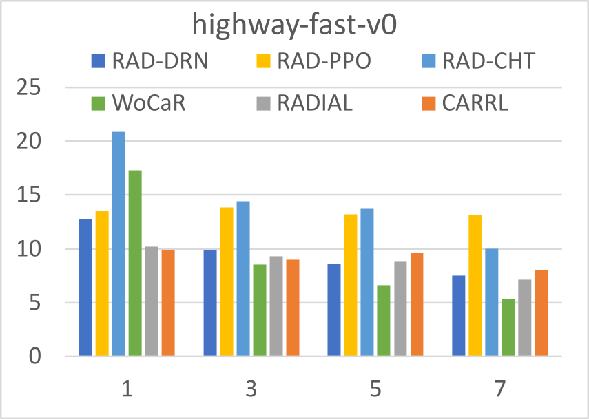
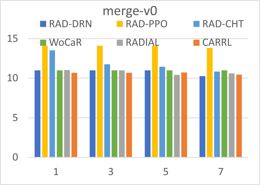
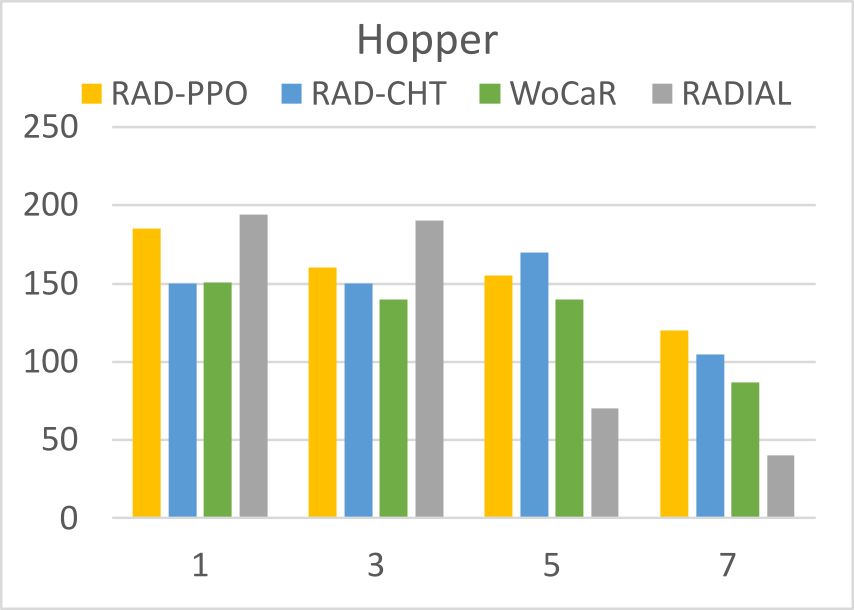
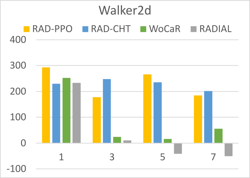
(a) Score vs. Percentile Perturbation Frequency with Strategically Timed Attack

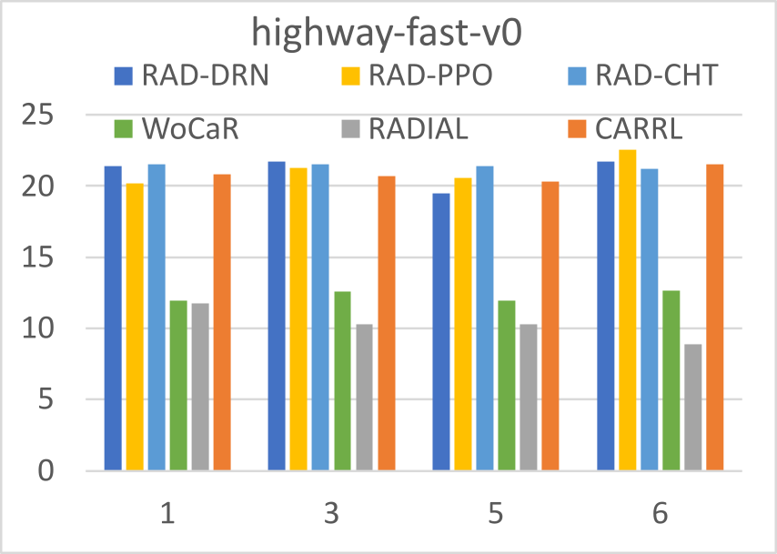
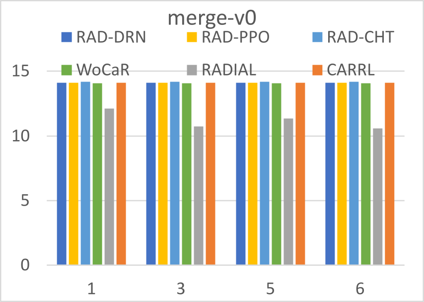
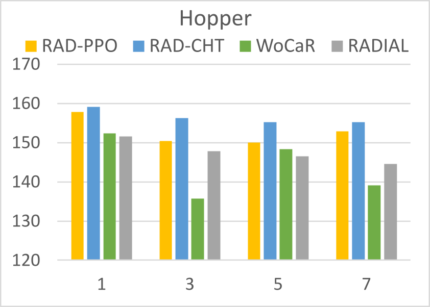
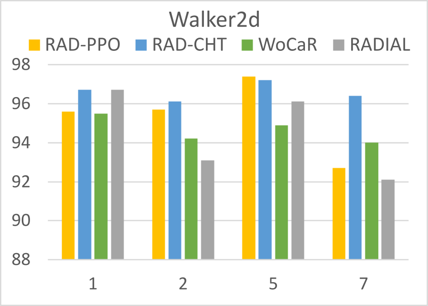
(b) Score vs. Percentile Perturbation Magnitude with Critical Point Attack

Figure 2: The performance of robust RL methods against strategic adversaries. The y-axis represents the score and the x-axis represents the intensity of the attack.

5.3 Results

In each table, we report the mean return over 50 random seeds. The highest score in each environment is shown in boldface.

Highway Domains: We report scores under PGD and WC attacks in Table 6. We observe that although the unperturbed performance of RAD- methods is lower than that of the vanilla solutions, all three approaches (RAD-DRN, RAD-PPO, and RAD-CHT) are extremely robust under different attacks and have higher performance than all other robust approaches in all of the Highway environments. We see that even though maximin methods (CARRL, WoCaR) are clearly well-suited to some scenarios, RAD- methods still outperform them.

MuJoCo Domains: Table 5 reports the results on MuJoCo, playing three commonly tested environments seen in comparison literature (Oikarinen et al. 2021; Liang et al. 2022). As the MuJoCo domains have continuous actions, we exclude value iteration-based methods (DQN, CARRL, and RAD-DRN) due to their inapplicability. We directly integrated our proposed techniques into the implementation from (Liang et al. 2022). Our assessment covers the MAD attack (Zhang et al. 2020) with a testing $\epsilon=0.15$, which marks the value at which we start observing deviations in the returns of the robustly trained agents. In addition, we subject the agents to PGD attacks with $\epsilon=\frac{5}{255}$.

Even in these problem settings, while RAD approaches do not provide the highest unperturbed performance (but are close to the best one), they (RAD-PPO and RAD-CHT) provide the best overall performance of all the approaches.

Atari Domains: We report results on four Atari domains used in preceding works (Liang et al. 2022; Oikarinen et al. 2021) in Table 7. RAD-PPO outperforms other robustness methods in nearly all attacks. RAD-DRN performs similarly to RAD-PPO, though faces some limitations in scenarios where rewards are sparse or mostly similar, such as in Pong. Regret measures the difference between outcomes, so training is more difficult when rewards are the same regardless of action. Interestingly, RAD-PPO does not suffer in this way, which we attribute to the superiority of the PPO framework over value iterative methods.

We exclude RAD-CHT from the Atari experiments, as the memory requirements to simultaneously hold models for all levels are outside the limitations of our hardware.

Strategic Attacks: Unlike previous works in robust RL, we also test our methods against attackers with a longer planning horizon than the above-mentioned greedy adversaries. In Figure 4, we test under a) the Strategically Timed Attack (Lin et al. 2017) and b) the Critical Point attack (Sun et al. 2020). We observe that across all domains, regret defense outperforms other robustness methods. Particularly, regularization methods fail with increasing rates as the strength or frequency of the attacks increases, even as maximin methods (CARRL) retain some level of robustness. This is one of the main advantages of our proposed methods, as the resulting policies seek robust trajectories to occupy rather than robust single-step action distributions.

6 Conclusion

We show that regret can be used to increase the robustness of RL to adversarial observations, even against stronger or previously unseen attackers. We propose an approximation of regret, CCER, and demonstrate its usefulness in proactive value iterative and policy gradient methods, and reactive training under CHT. Our results on a wide variety of problems (some more in Appendix B) show that regret-based defense significantly improves robustness against strong observation attacks from both greedy and strategic adversaries. Specifically, RAD-PPO performs the best on average across all (including the ones in Appendix B) of our experimental results.

Appendix A: Proofs

Proof of Proposition 1

Proof.

Since $\pi^{\bot}$ is optimal for all states from time step $t+1$:

$$\delta_{\texttt{CCER}}^{\pi^{\bot}_{[t+1,H]}}(z_{t+1}) \leq\delta_{\texttt{CCER}}^{\pi_{[t+1,H]}}(z_{t+1})$$ (8)

Therefore, we obtain:

$$\delta_{\texttt{CCER}}^{\left<\pi_{t},\pi^{\bot}_{[t+1,H]}\right>}\!(z_{t})\!=\!R(z_{t},\pi_{t}(z_{t}))-\min\nolimits_{s_{t}\in N({{z}_{t}})}\!R(s_{t},\pi_{t}(z_{t}))$$

$$\qquad\qquad\qquad\qquad+\gamma\mathbb{E}_{z_{t+1}}\Big{[}\delta_{\texttt{CCER}}^{\pi^{\bot}_{[t+1,H]}}(z_{t+1})\Big{]}$$

$$\qquad\quad\leq R(z_{t},\pi_{t}(z_{t}))-\min\nolimits_{s_{t}\in N({{z}_{t}})}R(s_{t},\pi_{t}(z_{t}))$$ (9)

$$\qquad\qquad\qquad\qquad+\gamma E_{z_{t+1}}[\delta_{\texttt{CCER}}^{\pi_{[t+1,H]}}(z_{t+1})]$$

$$\qquad\quad\leq\delta_{\texttt{CCER}}^{\pi_{t},\pi_{[t+1,H]}}(z_{t+1})$$ (10)

which concludes our proof. ∎

Proof of Proposition 2

Proof.

We have:

$$\frac{\partial\delta_{\texttt{CCER}}^{\pi_{\theta}}(z)}{\partial\theta}=\frac{\partial}{\partial\theta}\sum\nolimits_{a}\pi_{\theta}(z,a)\delta_{\texttt{CCER}}^{\pi_{\theta}}(z,a)$$

$$=\!\!\sum\nolimits_{a}\!\!\Big{[}\frac{\partial\pi_{\theta}(z,a)}{\partial\theta}\delta_{\texttt{CCER}}^{\pi_{\theta}}(z,a)\!+\!\pi_{\theta}(z,a)\!\Big{[}\frac{\partial}{\partial\theta}\delta_{\texttt{CCER}}^{\pi_{\theta}}(z,a)\Big{]}\Big{]}$$

$$=\!\!\sum\nolimits_{a}\!\!\Big{[}\frac{\partial\pi_{\theta}(z,a)}{\partial\theta}\delta_{\texttt{CCER}}^{\pi_{\theta}}(z,a)\!+\!\pi_{\theta}(z,a)\!\Big{[}\!\sum\nolimits_{z^{\prime}}\!\!\gamma\frac{\partial}{\partial\theta}\delta_{\texttt{CCER}}^{\pi_{\theta}}(z^{\prime})\Big{]}\Big{]}$$

After unrolling this equation, and adjusting terms, we obtain the following overall gradient computation:

$$\frac{\partial\delta_{\texttt{CCER}}^{\pi_{\theta}}(z)}{\partial\theta} \!=\!\sum\nolimits_{z}\!\!P(z|\pi_{\theta})\!\sum\nolimits_{a}\!\!\frac{\partial\pi_{\theta}(z,a)}{\partial\theta}\delta_{\texttt{CCER}}^{\pi_{\theta}}(z,a)$$ (11)

which concludes our proof. ∎

Proof of Proposition 3

Proof.

We elaborate the objective function of the adversary as an expectation over all possible trajectories as follows:

$$V_{\mu_{\theta}}=\sum\nolimits_{i}P^{(k)}(i)\sum\nolimits_{\tau}P^{(i)}(\tau)R(\tau)$$

where the probability of a trajectory is computed as:

$$P^{(i)}(\tau)=\prod\nolimits_{t}\mu_{\theta}(z_{t}\mid s_{t})\pi^{(i)}(a_{t}\mid z_{t})P(s_{t+1}\mid s_{t},a_{t})$$

Therefore, we can compute the gradient $\nabla_{\theta}V_{\mu_{\theta}}$ as follows:

$$\sum\nolimits_{i}P^{(k)}(i)\sum\nolimits_{\tau}R(\tau)\nabla_{\tau}P^{(i)}(\tau)$$

$$=\sum\nolimits_{i}P^{(k)}(i)\sum\nolimits_{\tau}P^{(i)}(\tau)R(\tau)\nabla_{\theta}\log P^{(i)}(\tau)$$

$$=\sum\nolimits_{i}P^{(k)}(i)\sum\nolimits_{\tau}P^{(i)}(\tau)R(\tau)\sum\nolimits_{t}\nabla_{\theta}\log\mu_{\theta}(z_{t}|s_{t})$$

$$=\mathbb{E}_{i\sim P^{(k)}(i),\tau\sim(\mu_{\theta},\pi^{(i)},T)}\Big{[}R(\tau)\sum\nolimits_{t}\nabla_{\theta}\log\mu_{\theta}(z_{t}|s_{t})\Big{]}$$

which concludes our proof. ∎

Appendix B: More Results

6.1 Main Results Extended

Here we include our experimental results in their entirety; Some were removed to meet submission requirements.

Table 5: Results on MuJoCo. Each row shows the mean scores of each RL method against different attacks.

Algorithm	Unperturbed	MAD $\epsilon\!\!=\!0.15$	PGD $\epsilon\!\!=\!\frac{5}{255}$
Hopper
PPO	2741 $\pm$ 104	970$\pm$19	36$\pm$156
RADIAL	3737$\pm$75	2401$\pm$13	3070$\pm$31
WoCaR	3136$\pm$463	1510 $\pm$ 519	2647 $\pm$310
RAD-PPO	3473$\pm$23	2783$\pm$325	3110$\pm$30
RAD-CHT	3506$\pm$377	2910$\pm$ 699	3055 $\pm$152
HalfCheetah
PPO	5566 $\pm$ 12	1483$\pm$20	-27$\pm$1308
RADIAL	4724$\pm$76	4008$\pm$450	3911$\pm$129
WoCaR	3993$\pm$152	3530$\pm$458	3475$\pm$610
RAD-PPO	4426$\pm$54	4240$\pm$4	4022$\pm$851
RAD-CHT	4230$\pm$140	4180$\pm$37	3934$\pm$486
Walker2d
PPO	3635 $\pm$ 12	680$\pm$1570	730$\pm$262
RADIAL	5251$\pm$10	3895$\pm$128	3480$\pm$3.1
WoCaR	4594$\pm$974	3928$\pm$1305	3944$\pm$508
RAD-PPO	4743$\pm$78	3922$\pm$426	4136$\pm$639
RAD-CHT	4790$\pm$61	4228$\pm$539	4009$\pm$516

Table 6: Results on Highway. Each row shows the mean scores of each RL method against different attacks.

Algorithm	Unperturbed	WC Policy	PGD, $\epsilon\!\!=\!\frac{3}{255}$
highway-fast-v0
DQN	24.91$\pm$20.27	3.68$\pm$35.41	15.71$\pm$13
PPO	22.8$\pm$5.42	13.63$\pm$19.85	15.21$\pm$16.1
CARRL	24.4$\pm$1.10	4.86$\pm$15.4	12.43$\pm$3.4
RADIAL	28.55$\pm$0.01	2.42$\pm$1.3	14.97$\pm$3.1
WoCaR	21.49$\pm$0.01	6.15$\pm$0.3	6.19$\pm$0.4
RAD-DRN	24.85$\pm$0.01	22.65$\pm$0.02	18.8$\pm$24.6
RAD-PPO	21.01$\pm$1.23	20.59$\pm$4.10	20.02$\pm$0.01
RAD-CHT	21.83 $\pm$ 0.35	21.1 $\pm$ 0.24	21.48 $\pm$ 1.8
merge-v0
DQN	14.83$\pm$0.0	6.97$\pm$0.03	10.82$\pm$2.85
PPO	11.08$\pm$0.01	10.2$\pm$0.02	10.42$\pm$0.95
CARRL	12.6$\pm$0.01	12.6$\pm$0.01	12.02$\pm$0.01
RADIAL	14.86$\pm$0.01	11.29$\pm$0.01	11.04$\pm$0.91
WoCaR	14.91$\pm$0.04	12.01$\pm$0.28	11.71$\pm$0.21
RAD-DRN	14.86$\pm$0.01	13.23$\pm$0.01	11.77$\pm$1.07
RAD-PPO	13.91$\pm$0.01	13.90$\pm$0.01	11.72$\pm$0.01
RAD-CHT	14.7 $\pm$ 0.01	14.7 $\pm$ 0.12	13.01 $\pm$ 0.32
roundabout-v0
DQN	9.55$\pm$0.081	8.97$\pm$0.26	9.01$\pm$1.9
PPO	10.33$\pm$0.40	9.23$\pm$0.69	9.09$\pm$1.35
CARRL	9.75$\pm$0.01	9.75$\pm$0.01	5.92$\pm$0.12
RADIAL	10.29$\pm$0.01	5.33$\pm$7e-31	8.77$\pm$2.4
WoCaR	6.75$\pm$2.5	6.05$\pm$0.14	6.48$\pm$2.7
DRN	10.39$\pm$0.01	9.33$\pm$3e-30	9.18$\pm$2.1
RAD-PPO	9.22$\pm$0.3	8.98$\pm$0.3	9.11$\pm$0.3
RAD-CHT	9.79 $\pm$ 0.02	9.12 $\pm$ 0.01	9.5 $\pm$ 0.9
intersection-v0
DQN	9.9$\pm$0.49	1.31$\pm$2.85	8.61$\pm$0.1
PPO	9.26$\pm$7.6	3.62$\pm$11.63	6.75$\pm$12.93
RADIAL	10.0$\pm$0	2.4$\pm$5.1	9.61$\pm$0.1
WoCaR	10.0$\pm$0.05	9.47$\pm$0.3	3.26$\pm$0.4
CARRL	8.0$\pm$0	7.5$\pm$0	9.0$\pm$0.1
DRN	10.0$\pm$0	10.0$\pm$0	9.68$\pm$0.1
RAD-PPO	9.85$\pm$1.2	9.71$\pm$2.3	9.62$\pm$0.1
RAD-CHT	4.52 $\pm$ 1.9	4.50 $\pm$ 2.5	4.67 $\pm$ 3.1

Table 7: Results on Atari. Each row shows the mean scores of each RL method against different attacks.

Algorithm	Unperturbed	WC Policy	PGD $\epsilon\!\!=\!\frac{5}{255}$
Pong
DQN	21.0$\pm$0	-21.0$\pm$0.0	-21.0$\pm$0.0
PPO	21.0$\pm$0	-20.0$\pm$ 0.07	-19.0$\pm$1.0
CARRL	13.0 $\pm$1.2	11.0$\pm$0.010	6.0$\pm$1.2
RADIAL	21.0$\pm$0	11.0$\pm$2.9	21.0$\pm$ 0.01
WoCaR	21.0$\pm$0	18.7 $\pm$0.10	20.0 $\pm$ 0.21
RAD-DRN	21.0$\pm$0	14.0 $\pm$ 0.04	14.0 $\pm$ 2.40
RAD-PPO	21.0$\pm$0	20.1$\pm$1.0	20.8$\pm$0.02
Freeway
DQN	33.9$\pm$0.10	0$\pm$0.0	2$\pm$1.10
PPO	29 $\pm$ 3.0	4 $\pm$ 2.31	2$\pm$2.0
CARRL	18.5$\pm$0.0	19.1 $\pm$1.20	15.4$\pm$0.22
RADIAL	33.2$\pm$0.19	29.0$\pm$1.1	24.0$\pm$0.10
WoCaR	31.2$\pm$0.41	19.8$\pm$3.81	28.1$\pm$3.24
RAD-DRN	33.2$\pm$0.18	30.0$\pm$0.23	27.7$\pm$1.51
RAD-PPO	33.0 $\pm$0.12	30.0$\pm$0.10	29 $\pm$0.12
BankHeist
DQN	1325$\pm$5	0$\pm$0	0.4$\pm$55
PPO	1350$\pm$0.1	680$\pm$419	0$\pm$116
CARRL	849$\pm$0	830$\pm$32	790$\pm$110
RADIAL	1349$\pm$0	997$\pm$3	1130$\pm$6
WoCaR	1220$\pm$0	1207$\pm$39	1154$\pm$94
RAD-DRN	1340$\pm$0	1170$\pm$42	1211$\pm$56
RAD-PPO	1340$\pm 0$	1301$\pm$8	1335$\pm$52
RoadRunner
DQN	43380 $\pm$860	1193 $\pm$259	3940 $\pm$ 92
PPO	42970$\pm$210	18309$\pm$485	10003$\pm$521
CARRL	26510$\pm$20	24480$\pm$ 200	22100$\pm$370
RADIAL	44501$\pm$1360	23119$\pm$1100	24300$\pm$1315
WoCaR	44156$\pm$2270	25570$\pm$390	12750$\pm$405
RAD-DRN	42900$\pm$1020	29090$\pm$440	27150$\pm$505
RAD-PPO	42805$\pm$240	33960$\pm$360	33990$\pm$403

6.2 Strategic Attacks

In Figure 4 we report the effect of multi-step strategic attacks against robustly trained RL agents. In addition to the results presented in the main paper, we also include results on Atari domains.

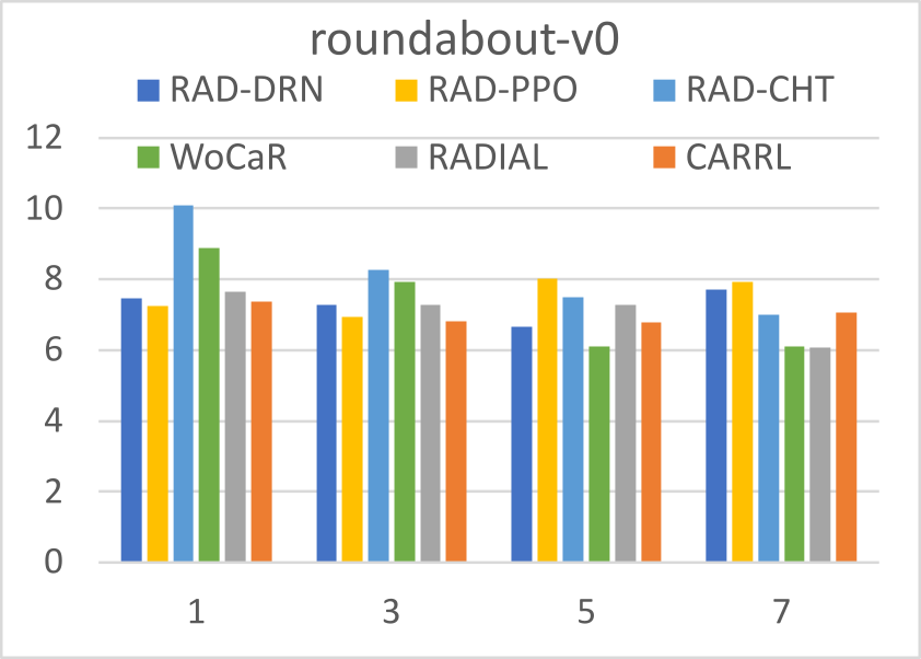
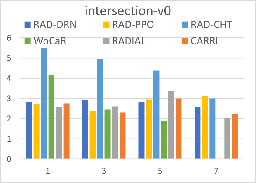
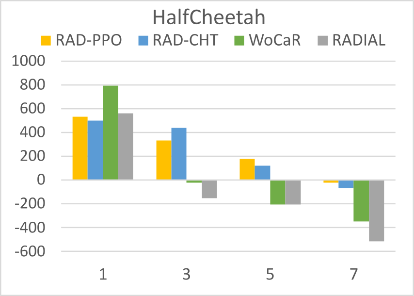
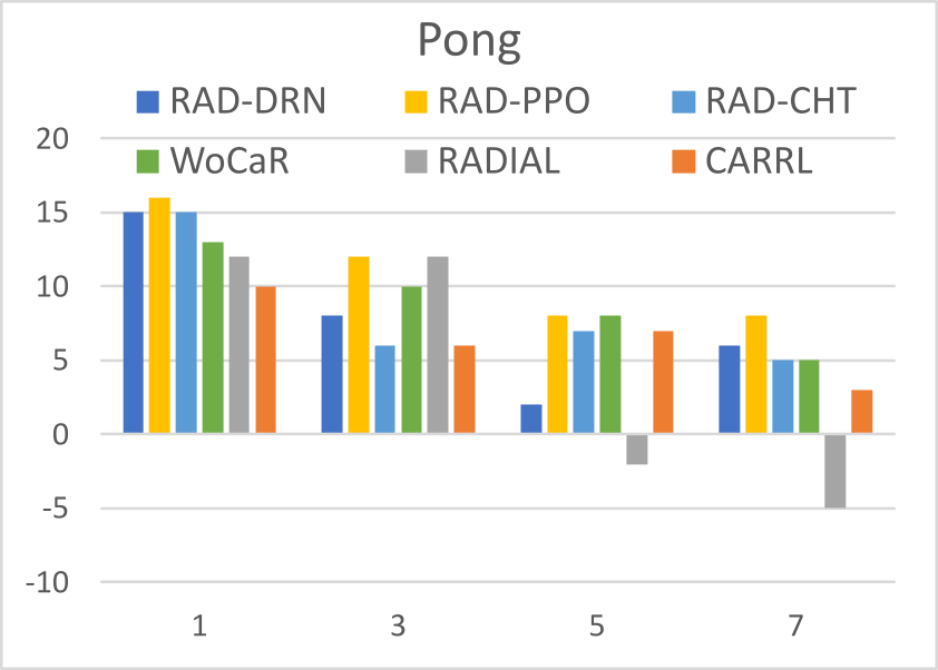
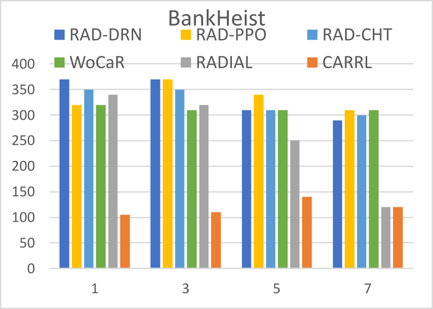
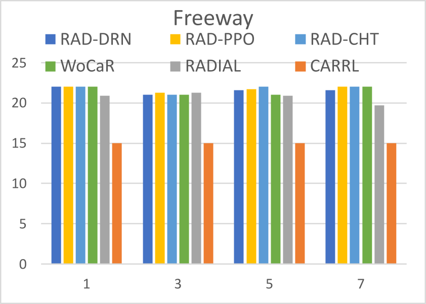
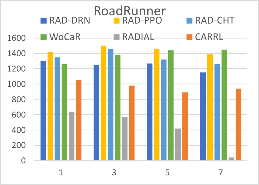
(a) Score vs. Percentile Perturbation Frequency with Strategically Timed Attack

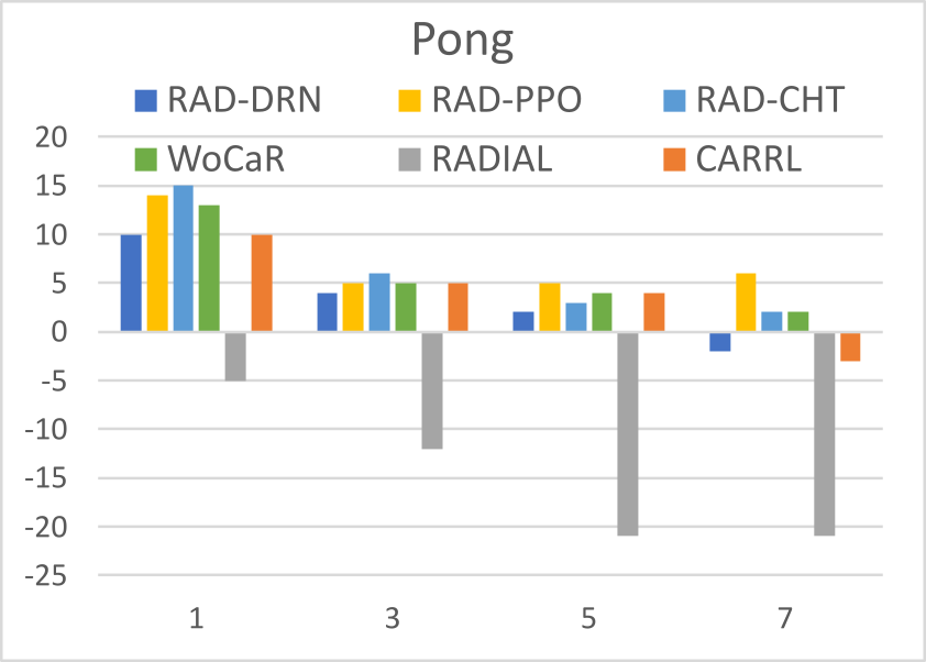
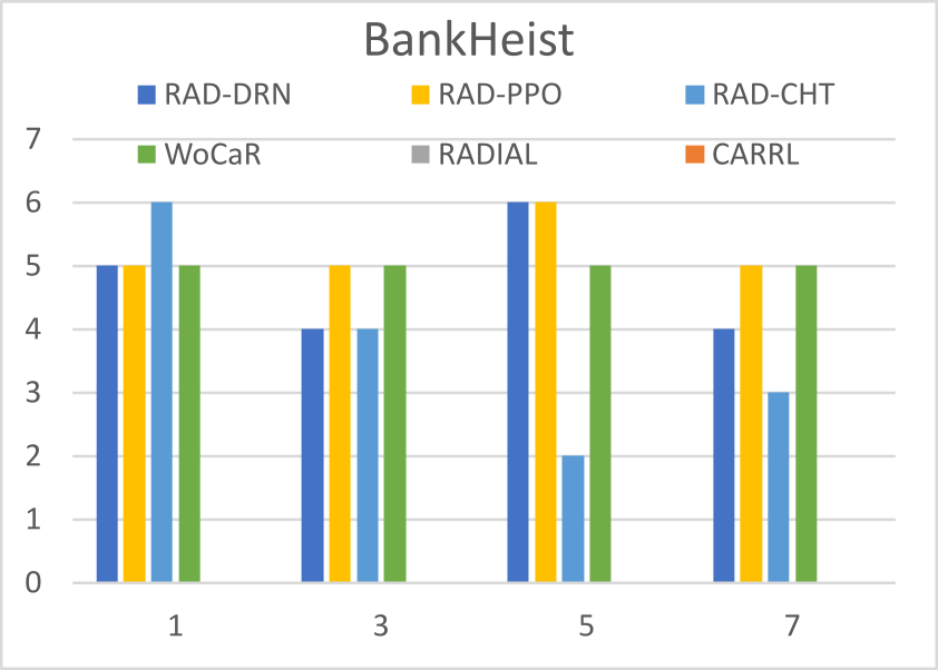
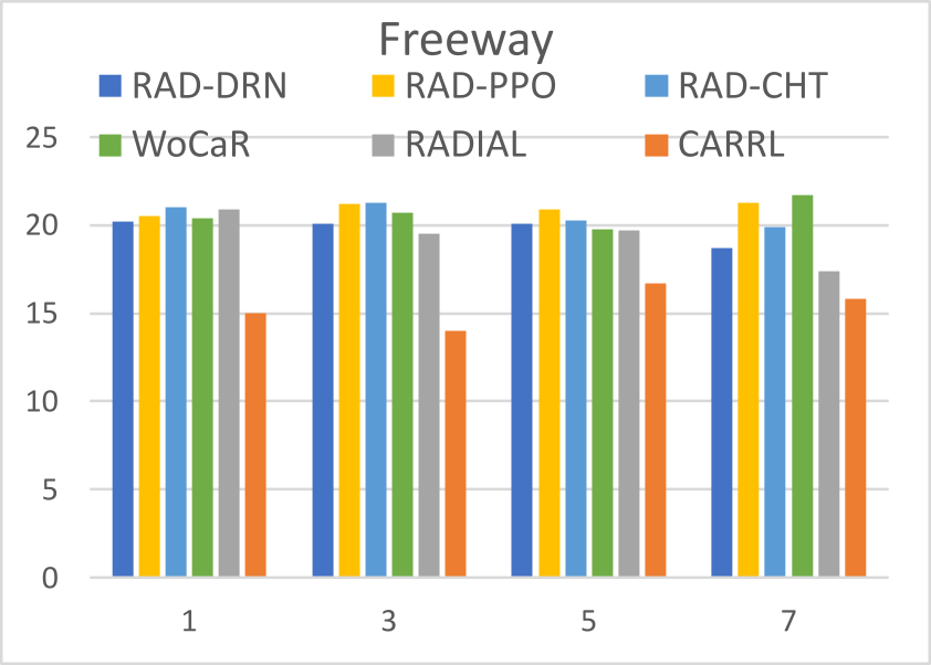
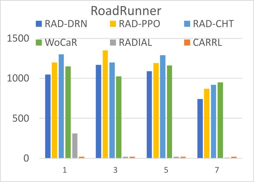
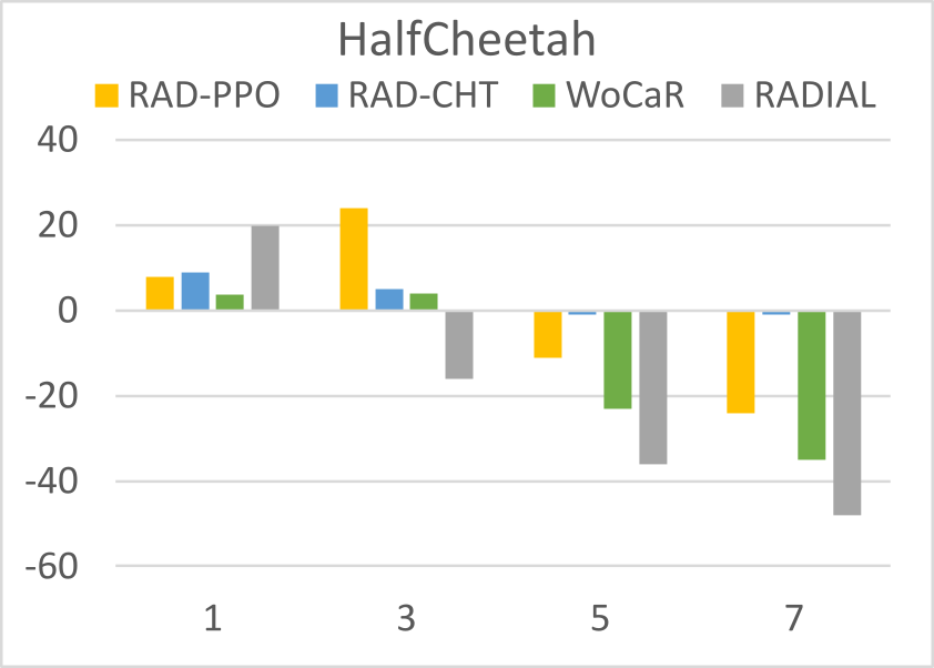
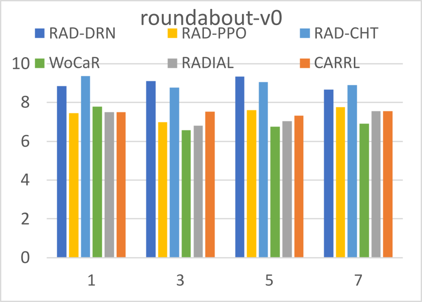
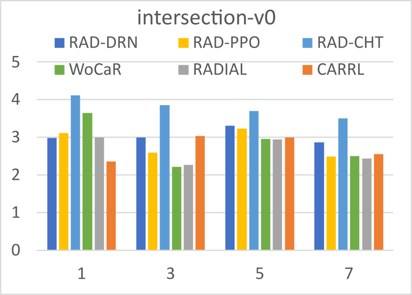
(b) Score vs. Percentile Perturbation Magnitude with Critical Point Attack

Figure 4: The performance of robust RL methods against strategic adversaries. The y-axis represents the score and the x-axis represents the intensity of the attack.

Appendix C: Training Details and Hyperparameters

6.3 Model Architecture

Our RAD-DRN model follows commonly found settings for a simple DQN: a linear input layer, a 64x hidden layer, and a fully connected output layer. For images, we instead use a convolutional layer with an 8x8 kernel, stride of 4 and 32 channels, a convolutional layer with a 4x4 kernel, stride of 2 and 64 channels, and a final convolutional layer with a 3x3 kernel, stride of 1 and 64 channels (this is the same setup as RADIAL and WoCaR implementations). Each layer is followed by a ReLU activation, and finally feeds into a fully connected output.

Our RAD-PPO model is built on the standard implementation in StableBaselines3 PPO, with [256,256] MLP network parameters for non-image tasks and [512,512] CNN parameters for Atari domains. To maintain an estimate of the minimum reward to calculate regret, we attach a DQN as constructed above.

Worst-case policy attack models are also DQN models as described above, with the output layer size (i.e. number of actions) corresponding to the size of the attack neighborhood.

6.4 Regarding Neighborhoods

In our paper, we commonly reference the neighborhood $N(z_{t})$ surrounding the observed state $z_{t}$; This is akin to the $L_{p}$-ball around $z_{t}$. In our experiments, we use an $L_{p}$-ball of radius $\epsilon=3/255$, and sample 10 states to create our neighborhood. We selected the sample size 10 after trying [2,5,10,20] and finding 10 to be sufficient without noticeably impacting computation speed. We also note that changing $\epsilon$ to $2/255$ or $5/255$ has little impact on the final performance of the model.

6.5 Training Details

We train our models for 3000 episodes ( 10k frames) on highway environments and 1000 episodes (3 million frames) on Atari environments; For MuJoCo simulations, we find 200,000 frames to be sufficient. RAD-DRN learning rates are set to $5e-4$ for all environments (tuned from a range $[1e-3,3e-4,5e-4,5e-5,5e-7]$, while RAD-PPO uses the default parameters of StableBaselines3’s PPO implementation. Worst-case adversaries are trained very briefly as they are solving a rather simple MDP, we use $10,000$ frames for both highway and Atari environments and use a learning rate of $0.05$

6.6 Testing Details

During the testing of our models, we repeat our experiments 10 times each for 50 random seeds, for a total of 500 episodes in a test.

During testing, adversary agents are permitted to make perturbations every $t_{adv}$ steps, to reduce the rate of critical failure (which is unhelpful to the evaluation of the methods). Our experiments on highway environments are conducted with $t_{adv}=2$, and $t_{adv}=5$ on Atari domains. To remove temporal dependence, this interval is shifted by one between testing episodes—the victim is tested against perturbations at every step at least once, but not every step in a single episode.

References

- Ahmed et al. (2013) Ahmed, A.; Varakantham, P.; Adulyasak, Y.; and Jaillet, P. 2013. Regret based robust solutions for uncertain Markov decision processes.
- Andriushchenko and Flammarion (2020) Andriushchenko, M.; and Flammarion, N. 2020. Understanding and improving fast adversarial training. Advances in Neural Information Processing Systems, 33: 16048–16059.
- Bai et al. (2021) Bai, T.; Luo, J.; Zhao, J.; Wen, B.; and Wang, Q. 2021. Recent advances in adversarial training for adversarial robustness. arXiv preprint arXiv:2102.01356.
- Bai, Guan, and Wang (2019) Bai, X.; Guan, J.; and Wang, H. 2019. A model-based reinforcement learning with adversarial training for online recommendation. Advances in Neural Information Processing Systems, 32.
- Bellemare et al. (2013) Bellemare, M. G.; Naddaf, Y.; Veness, J.; and Bowling, M. 2013. The Arcade Learning Environment: An Evaluation Platform for General Agents. Journal of Artificial Intelligence Research, 47: 253–279.
- Camerer, Ho, and Chong (2004) Camerer, C. F.; Ho, T.-H.; and Chong, J.-K. 2004. A cognitive hierarchy model of games. The Quarterly Journal of Economics, 119(3): 861–898.
- Chen et al. (2018) Chen, S.; Cornelius, C.; Martin, J.; and Chau, D. H. 2018. Robust Physical Adversarial Attack on Faster R-CNN Object Detector. CoRR, abs/1804.05810.
- Everett, Lütjens, and How (2020) Everett, M.; Lütjens, B.; and How, J. P. 2020. Certified Adversarial Robustness for Deep Reinforcement Learning. CoRR, abs/2004.06496.
- Ganin et al. (2016) Ganin, Y.; Ustinova, E.; Ajakan, H.; Germain, P.; Larochelle, H.; Laviolette, F.; Marchand, M.; and Lempitsky, V. 2016. Domain-adversarial training of neural networks. The journal of machine learning research, 17(1): 2096–2030.
- Gleave et al. (2019) Gleave, A.; Dennis, M.; Wild, C.; Kant, N.; Levine, S.; and Russell, S. 2019. Adversarial Policies: Attacking Deep Reinforcement Learning.
- Goodfellow, Shlens, and Szegedy (2014) Goodfellow, I. J.; Shlens, J.; and Szegedy, C. 2014. Explaining and Harnessing Adversarial Examples.
- Huang et al. (2017) Huang, S.; Papernot, N.; Goodfellow, I.; Duan, Y.; and Abbeel, P. 2017. Adversarial Attacks on Neural Network Policies.
- Jin, Keutzer, and Levine (2018) Jin, P.; Keutzer, K.; and Levine, S. 2018. Regret minimization for partially observable deep reinforcement learning.
- Kamalaruban et al. (2020) Kamalaruban, P.; Huang, Y.-T.; Hsieh, Y.-P.; Rolland, P.; Shi, C.; and Cevher, V. 2020. Robust reinforcement learning via adversarial training with langevin dynamics. Advances in Neural Information Processing Systems, 33: 8127–8138.
- Kang et al. (2019) Kang, D.; Sun, Y.; Brown, T.; Hendrycks, D.; and Steinhardt, J. 2019. Transfer of adversarial robustness between perturbation types. arXiv preprint arXiv:1905.01034.
- Kiran et al. (2021) Kiran, B. R.; Sobh, I.; Talpaert, V.; Mannion, P.; Al Sallab, A. A.; Yogamani, S.; and Pérez, P. 2021. Deep reinforcement learning for autonomous driving: A survey.
- Kos and Song (2017) Kos, J.; and Song, D. 2017. Delving into adversarial attacks on deep policies.
- Leurent (2018) Leurent, E. 2018. An Environment for Autonomous Driving Decision-Making. https://github.com/eleurent/highway-env.
- Liang et al. (2022) Liang, Y.; Sun, Y.; Zheng, R.; and Huang, F. 2022. Efficient adversarial training without attacking: Worst-case-aware robust reinforcement learning. Advances in Neural Information Processing Systems, 35: 22547–22561.
- Lin et al. (2017) Lin, Y.; Hong, Z.; Liao, Y.; Shih, M.; Liu, M.; and Sun, M. 2017. Tactics of Adversarial Attack on Deep Reinforcement Learning Agents. CoRR, abs/1703.06748.
- Madry et al. (2017) Madry, A.; Makelov, A.; Schmidt, L.; Tsipras, D.; and Vladu, A. 2017. Towards Deep Learning Models Resistant to Adversarial Attacks.
- Mnih et al. (2013) Mnih, V.; Kavukcuoglu, K.; Silver, D.; Graves, A.; Antonoglou, I.; Wierstra, D.; and Riedmiller, M. 2013. Playing Atari with Deep Reinforcement Learning.
- Mnih et al. (2015) Mnih, V.; Kavukcuoglu, K.; Silver, D.; Rusu, A. A.; Veness, J.; Bellemare, M. G.; Graves, A.; Riedmiller, M.; Fidjeland, A. K.; Ostrovski, G.; et al. 2015. Human-level control through deep reinforcement learning. nature, 518(7540): 529–533.
- Oikarinen et al. (2021) Oikarinen, T.; Zhang, W.; Megretski, A.; Daniel, L.; and Weng, T.-W. 2021. Robust Deep Reinforcement Learning through Adversarial Loss.
- Pattanaik et al. (2017) Pattanaik, A.; Tang, Z.; Liu, S.; Bommannan, G.; and Chowdhary, G. 2017. Robust deep reinforcement learning with adversarial attacks.
- Pinto et al. (2017) Pinto, L.; Davidson, J.; Sukthankar, R.; and Gupta, A. 2017. Robust adversarial reinforcement learning. In International Conference on Machine Learning, 2817–2826. PMLR.
- Rajeswaran et al. (2017) Rajeswaran, A.; Ghotra, S.; Ravindran, B.; and Levine, S. 2017. EPOpt: Learning Robust Neural Network Policies Using Model Ensembles. arXiv:1610.01283.
- Rigter, Lacerda, and Hawes (2021) Rigter, M.; Lacerda, B.; and Hawes, N. 2021. Minimax Regret Optimisation for Robust Planning in Uncertain Markov Decision Processes.
- Schulman et al. (2017) Schulman, J.; Wolski, F.; Dhariwal, P.; Radford, A.; and Klimov, O. 2017. Proximal Policy Optimization Algorithms.
- Shafahi et al. (2019) Shafahi, A.; Najibi, M.; Ghiasi, M. A.; Xu, Z.; Dickerson, J.; Studer, C.; Davis, L. S.; Taylor, G.; and Goldstein, T. 2019. Adversarial training for free! Advances in Neural Information Processing Systems, 32.
- Shafahi et al. (2020) Shafahi, A.; Najibi, M.; Xu, Z.; Dickerson, J.; Davis, L. S.; and Goldstein, T. 2020. Universal adversarial training. In Proceedings of the AAAI Conference on Artificial Intelligence, volume 34, 5636–5643.
- Spielberg et al. (2019) Spielberg, S.; Tulsyan, A.; Lawrence, N. P.; Loewen, P. D.; and Bhushan Gopaluni, R. 2019. Toward self-driving processes: A deep reinforcement learning approach to control.
- Sun et al. (2020) Sun, J.; Zhang, T.; Xie, X.; Ma, L.; Zheng, Y.; Chen, K.; and Liu, Y. 2020. Stealthy and Efficient Adversarial Attacks against Deep Reinforcement Learning.
- Sun et al. (2023) Sun, Y.; Zheng, R.; Liang, Y.; and Huang, F. 2023. Who Is the Strongest Enemy? Towards Optimal and Efficient Evasion Attacks in Deep RL. arXiv:2106.05087.
- Tan et al. (2020) Tan, K. L.; Esfandiari, Y.; Lee, X. Y.; Sarkar, S.; et al. 2020. Robustifying reinforcement learning agents via action space adversarial training. In 2020 American control conference (ACC), 3959–3964. IEEE.
- Todorov, Erez, and Tassa (2012) Todorov, E.; Erez, T.; and Tassa, Y. 2012. MuJoCo: A physics engine for model-based control. In 2012 IEEE/RSJ International Conference on Intelligent Robots and Systems, 5026–5033. IEEE.
- Wong, Rice, and Kolter (2020) Wong, E.; Rice, L.; and Kolter, J. Z. 2020. Fast is better than free: Revisiting adversarial training. arXiv preprint arXiv:2001.03994.
- Zhang et al. (2020) Zhang, H.; Chen, H.; Xiao, C.; Li, B.; Liu, M.; Boning, D.; and Hsieh, C.-J. 2020. Robust Deep Reinforcement Learning against Adversarial Perturbations on State Observations.